Embed Size (px)
Citation preview

STEERING CONTROL MECHANISM
AJMAL HUSSAIN (ME10B001)
AKASH SUBUDHI (ME10B002)
ALBIN ABRAHAM (ME10B003)
PAWAN KUMAR (ME10B023)
YOGITHA MALPOTH (ME10B024)
ZAID AHSAN (ME10B043)
SHANTI SWAROOP KANDALA (ME14RESCH01001)

OUTLINE
• Introduction
• Types of steering
• Cad models
• Role of cornering stiffness
• Lateral control system
• Electric power assisted steering
• Optimization using genetic algorithm
• Conclusion

INTRODUCTION
● Collection of components which allows to follow the desired course.
● In a car : ensure that wheels are pointing in the desired direction of motion.
● Convert rotary motion of the steering to the angular turn of the wheel.
● Mechanical advantage is used in this case.
● The joints and the links should be adjusted with precision.
● Smallest error can be dangerous
● Mechanism should not transfer the shocks in the road to the driver's hands.
● It should minimize the wear on the tyres.

RACK AND PINION STEERING SYSTEM
The pinion moves the rack converting circular motion into linear motion along a different axis
Rack and pinion gives a good feedback there by imparts a feel to the driving
Most commonly used system in automobiles now.
Disadvantage of developing wear and there by backlash.

RECIRCULATING BALL
●Used in Older automobiles
●The steering wheel rotates the shaft which turns the worm gear.
●Worm gear is fixed to the block and this moves the wheels.
●More mechanical advantage.
●More strength and durable

POWER STEERING
● Too much physical exertion was needed for vehicles
● External power is only used to assist the steering effort.
● Power steering gives a feedback of forces acting on the front wheel to give a sense of how wheels
are interacting with the road.
● Hydraulic and electric systems were developed.
● Also hybrid hydraulic-electric systems were developed.
● Even if the power fails, driver can steer only it becomes more heavier.

COMPONENTS

ELECTRIC POWER STEERING
● Uses an electric motor to assist the driving
● Sensors detect the position of the steering column.
● An electronic module controls the effort to be applied depending on the conditions.
● The module can be customised to apply varying amounts of assistance depending on driving
conditions.
● The assistance can also be tuned depending on vehicle type, driver preferences

HYDRAULIC VS ELECTRIC
● Electric eliminates the problems of dealing with leakage and disposal of the hydraulic fluid.
● Another issue is that if the hydraulic system fails, the driver will have to spent more effort since he
has to turn the power assistance system as well as the vehicle using manual effort.
● Hydraulic pump must be run constantly where as electric power is used accordingly and is more
energy efficient.
● Hyrdraulic is more heavy, complicated, less durable and needs more maintenance.
● Hydraulic takes the power directly from the engine so less mileage.

SPEED SENSITIVE STEERING
● There is more assistance at lower speeds and less at higher speeds.
● Diravi is the first commercially available variable power steering system introduced by citroen.
● A centrifugal regulator driven by the secondary shaft of the gearbox gives a proportional
hydraulic pressure to the speed of the car
● This pressure acts on a cam directly revolving according to the steering wheel.
● This gives an artificial steering pressure by trying to turn back the steering to the central position
● Newer systems control the assistance directly
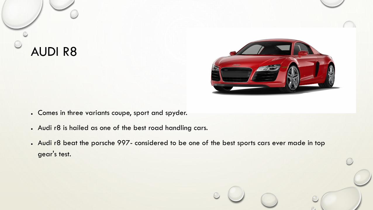
AUDI R8
● Comes in three variants coupe, sport and spyder.
● Audi r8 is hailed as one of the best road handling cars.
● Audi r8 beat the porsche 997- considered to be one of the best sports cars ever made in top
gear's test.


DYNAMIC ANALYSIS
tanβf = tanβ + hf r/ U cosβ
tanβr = tanβ + hr r/ U cosβ
αf = τ - βf;
αr = βr;
αf = τ - β - hf r/ U
αr = - β + hr r/ U hr


FINAL EQUATIONS

STATE SPACE EQUATIONS

The matrices of the state
space equations are given
The elements of these
matrices change due to
variation in C and load
The new matrices are
calculated
sys=ss(A,B,C,D)
The transfer functions are
then given by,
tf()sys
A(1,1)=-(Cr+Cf)/(m*U);
A(2,1)=(hr*Cr-hf*Cf)/J;
A(1,2)=-1+((hr*Cr-hf*Cf)/(m*(U^2)));
A(2,2)=-((hr^2)*Cr+(hf^2)*Cf)/(J*U);
B(1,1)=Cf/(m*U);
B(2,1)=hf*Cf/J;
C(1,1)=-((Cf+Cr)/m)+(ls*(hr*Cr-hf*Cf)/J);
C(1,2)=((hr*Cr-hf*Cf)/(m*U))-ls*(((hr^2)*Cr+(hf^2)*Cf)/(J*U));
C(2:3,1:2)=eye(2,2);
D(1,1)=(Cf/m)+ls*(hf*Cf/J);
sys=ss(A,B,C,D);
tf(sys)

STABLE AND UNSTABLE REGIONS VARYING CORNERING STIFFNESS
Stable region

M=3000 kg
Time Time Time
Slip
ang
le
Ya
w r
ate
Late
ral a
cc

M=4000 kg
Time Time Time
Slip
ang
le
Ya
w r
ate
Late
ral a
cc

M=5000 kg
Time Time Time
Slip
ang
le
Ya
w r
ate
Late
ral a
cc

RESULTS
Sl.No Vehicle
mass
Cornering
Stiffness
(kN/deg)
Settling Time
(sec) Peak
1. 1000 0.35
β 5.8 1.02
Yaw rate 3.4 1.04
Lateral acc. 10 No
overshoot
2. 2000 0.65
β 4.4 1.04
Yaw rate 4.3 1.05
Lateral acc. 7.19 1.11
3. 3000 0.92
β 3.5 1.04
Yaw rate 4.7 1.05
Lateral acc. 6.2 1.09

RESULTS
Sl.No Vehicle
mass
Cornering
Stiffness
(kN/deg)
Settling Time
(sec) Peak
1. 4000 1.15
β 3.9 1.05
Yaw rate 5.2 1.05
Lateral acc. 6.2 1.11
2. 5000 1.22
β 4.2 1.06
Yaw rate 5.7 1.06
Lateral acc. 6.8 1.13
3. 6000 1.25
β 4.3 1.06
Yaw rate 5.9 1.05
Lateral acc. 6.9 1.13


LATERAL CONTROL SYSTEM
• Control strategy: look-down reference system
• Sensor at the front bumper to measure the lateral displacement
• GPS to measure the heading orientation
• Firstly, the road curvature estimator is designed based on the steering angle, which has
steering angle and its derivative as two state variables for which an estimation algorithm is
employed whose input comes from the sensor and the GPS data
• The closed loop controller is used as a compensator to control the lateral dynamics
• Precise and real-time estimation of the lateral displacements w. R. T the road are
accomplished using the proposed control system

SINGLE TRACK DYNAMICS
2
41
4
2
21
44414241
24212221
.
.
.
0
00
,1000
0010
,,
b
g
bB
aaaa
aaaaAU
d
d
d
d
X
BUAXX
ref
f
sr
sr
sf
sf
srsftfftrrrftfftrr
tfsr
f
tfsf
f
sfsrsfsrsrsrsr
sfsfsfsrsfsrsf
llglclcgccglclcg
I
ll
Mcb
I
ll
Mcb
gI
ggll
gM
glga
gI
ggll
gM
glga
gI
gl
Mg
ga
gI
ggll
gM
glga
gI
ggll
gM
glga
gI
gl
Mg
ga
4
22
321
4121
4
31
4
21
44
4
31
4
2142
4
1
4
241
4
31
4
21
22
4
31
4
2122
4
1
4
221
),(),(),(
1,
1
)(,
)(,
)(,
)(,
)77.2856.12)(77.2856.12)(8.62(
80000)(
jsjsssA
Actuator Dynamics
Feedback Controller Dynamics
12
1
)(
12
1
)(
)()( Structure
1
2
1
2
2
Pr
2
1
2
1
2
2
2
Dsss
KsKsKsC
s
K
Dsss
KsKsKsC
sCsC
DrDDrr
IPfDfDDf
f
rf

CONTROL SYSTEM
Implementation of Control System
1
1
1
1
)(
^
^
.
^
.
^
^
^_^^
^
^
.
lX
U
d
d
d
d
X
XHdLUBXA
ref
f
sr
sr
sf
sf
srX
Lateral Position Estimation System

RESULTS
Simulation result for a speed 80mi/h on dry road (road adhesion factor of 1 )
• The lateral displacement result has no
overshoot and is well damped.
• The steering angle and road curvature
estimations are within accuracy
specifications.
• The estimation error of the steering angle
is approximately 8% and the curvature
estimation error is around 10%.

ELECTRIC POWER ASSISTED STEERING

EQUATIONS
Steering column, Driver torque
Road conditions and friction

Assist Motor Model
Rack and Pinion Displacement

CONTROL DIAGRAM

Speed 40kmph (without controller)
Ass
ist C
urre
nt (A
)
Time

Speed 40kmph (with controller)
Ass
ist C
urre
nt (A
)
Time

RESULTS
Sl.No Vehicle Speed Assist Current
(without PID)
Assist Current
(with PID)
1 40 0.16 0.14
2 50 0.24 0.19
3 60 0.28 0.24
4 70 0.33 0.29
5 80 0.38 0.34
6 90 0.62 0.55

Genetic Algorithm

GA QUICK OVERVIEW
• Developed: USA in the 1970’s
• Early names: J. Holland, K. Dejong, D. Goldberg
• Typically applied to:
• Discrete optimization
• Attributed features:
• Not too fast
• Good heuristic for combinatorial problems
• Special features:
• Traditionally emphasizes combining information from good parents (crossover)
• Many variants, e.g., Reproduction models, operators

SIMPLE GENETIC ALGORITHM produce an initial population of individuals
evaluate the fitness of all individuals
while termination condition not met do
select fitter individuals for reproduction
recombine between individuals
mutate individuals
evaluate the fitness of the modified individuals
generate a new population
End while

1-POINT CROSSOVER
• Choose a random point on the two parents
• Split parents at this crossover point
• Create children by exchanging tails
• Pc typically in range (0.6, 0.9)

MUTATION
• Alter each gene independently with a probability pm
• Pm is called the mutation rate
• Typically between 1/pop_size and 1/ chromosome_length

RESULTS

STABILITY ANALYSIS
• The vehicle model used in the analysis is a simple three degree of freedom
yaw plane representation with differential braking
𝑚𝑈𝑥 = 𝐹𝑥𝑟 + 𝐹𝑥𝑓cos𝜆 − 𝐹𝑦𝑓sin𝜆 + 𝑚𝑟𝑈𝑦
𝑚𝑈𝑦 = 𝐹𝑦𝑟 + 𝐹𝑥𝑓sin𝜆 + 𝐹𝑦𝑓cos𝜆 − 𝑚𝑟𝑈𝑥
𝐼𝑧𝑟 = 𝑎𝐹𝑥𝑓sin𝛿 + 𝑎𝐹𝑦𝑓cos𝛿 − 𝑏𝐹𝑦𝑟 +𝑑
2(𝛥𝐹𝑥𝑟 + 𝛥𝐹𝑥𝑓cos𝜆)

VEHICLE MODEL
𝐹𝑥𝑓 = 𝐹𝑥𝑟𝑓 + 𝐹𝑥𝑙𝑓
𝐹𝑥𝑟 = 𝐹𝑥𝑟𝑟 + 𝐹𝑥𝑙𝑟 𝛥𝐹𝑥𝑓 = 𝐹𝑥𝑟𝑓 − 𝐹𝑥𝑙𝑓
𝛥𝐹𝑥𝑟 = 𝐹𝑥𝑟𝑟 − 𝐹𝑥𝑙𝑟

EQUATIONS INVOLVED
• Assuming small angles and equal slip angles on the left and right wheels,
𝛼𝑓𝑟 =𝑈𝑦+𝑟𝑎
𝑈𝑥− 𝛿
𝛼𝑟 =𝑈𝑦 − 𝑟𝑏
𝑈𝑥
• Using a linear tire model, the lateral forces are given as
𝐹𝑦𝑓 = −𝐶𝑓𝛼𝑓
𝐹𝑦𝑟 = −𝐶𝑟𝛼𝑟

EQUATIONS INVOLVED
• Where Cf and Cr are the front and rear cornering stiffness's, respectively. Substituting the
expressions or the lateral forces into equations 1 through 3 and making small angle
approximations yields,
• 𝑚𝑈𝑥 = 𝑚𝑟𝑈𝑦 + 𝐹𝑥𝑟 + 𝐹𝑥𝑓 + 𝐶𝑓(𝑈𝑦+𝑟𝑎)
𝑈𝑥𝛿
• 𝑚𝑈𝑦 = −𝐶𝑟(𝑈𝑦−𝑟𝑏)
𝑈𝑥− 𝐶𝑓
(𝑈𝑦+𝑟𝑎)
𝑈𝑥−𝑚𝑟𝑈𝑥 + 𝐶𝑓𝛿 + 𝐹𝑥𝑓𝛿
• 𝐼𝑧𝑟 = 𝑎𝐹𝑥𝑓𝛿 − 𝑎𝐶𝑓(𝑈𝑦+𝑟𝑎)
𝑈𝑥+ 𝑏𝐶𝑟
(𝑈𝑦−𝑟𝑏)
𝑈𝑥+ 𝑎𝐶𝑓𝛿 +
𝑑
2(𝛥𝐹𝑥𝑟 + 𝛥𝐹𝑥𝑓)

EQUATIONS INVOLVED
• The linearization of a vehicle about a constant longitudinal velocity gives,
where
xAx .
..
eex
SI
CrbCfa
I
bCraCf
SI
bCraCf
mS
bCraCf
m
CrCf
mS
CrCf
A
zzz
)()()(0
1000
)()()(0
0010
22

STABILITY ANALYSIS
• Taking the determinant of yields the characteristic equation of the system
AI
02122 aa
mSI
mCbCaICrCa
z
rfzf )()( 22
1
2
22
2
)()(
mSI
mSaCbCbaCrCa
z
frf

STABLE AND UNSTABLE REGIONS VARYING CORNERING STIFFNESS
Stable oversteer region
Stable understeer region

LINEARIZATION WITHOUT VIRTUAL FORCE
mbCaC
baCCS
rf
rf
)(
)( 2
• In an oversteering case (aCf > bCr), the coefficient a2 will be negative when the
speed
• The critical speed obtained