Embed Size (px)
Citation preview
STEER-BY-WIRE: IMPLICATIONS FOR VEHICLE HANDLING AND SAFETY
a dissertation
submitted to the department of mechanical engineering
and the committee on graduate studies
of stanford university
in partial fulfillment of the requirements
for the degree of
doctor of philosophy
Paul Yih
January 2005

c© Copyright by Paul Yih 2005
All Rights Reserved
ii
I certify that I have read this dissertation and that, in
my opinion, it is fully adequate in scope and quality as a
dissertation for the degree of Doctor of Philosophy.
J. Christian Gerdes(Principal Adviser)
I certify that I have read this dissertation and that, in
my opinion, it is fully adequate in scope and quality as a
dissertation for the degree of Doctor of Philosophy.
Kenneth J. Waldron
I certify that I have read this dissertation and that, in
my opinion, it is fully adequate in scope and quality as a
dissertation for the degree of Doctor of Philosophy.
Stephen M. Rock(Aeronautics and Astronautics)
Approved for the University Committee on Graduate
Studies.
iii
This thesis is dedicated to the memory of Dr. Donald Streit.
iv
Abstract
Recent advances toward steer-by-wire technology have promised significant improve-
ments in vehicle handling performance and safety. While the complete separation of
the steering wheel from the road wheels provides exciting opportunities for vehicle
dynamics control, it also presents practical problems for steering control. This thesis
begins by addressing some of the issues associated with control of a steer-by-wire
system. Of critical importance is understanding how the tire self-aligning moment
acts as a disturbance on the steering system. A general steering control strategy has
been developed to emphasize the advantages of feedforward when dealing with these
known disturbances. The controller is implemented on a test vehicle that has been
converted to steer-by-wire.
One of the most attractive benefits of steer-by-wire is active steering capability.
When supplied with continuous knowledge of a vehicle’s dynamic behavior, active
steering can be used to modify the vehicle’s handling dynamics. One example pre-
sented and demonstrated in the thesis is the application of full vehicle state feedback
to augment the driver’s steering input. The overall effect is equivalent to changing a
vehicle’s front tire cornering stiffness. In doing so, it allows the driver to adjust a ve-
hicle’s fundamental handling characteristics and therefore precisely shift the balance
between responsiveness and safety.
Another benefit of steer-by-wire is the availability of steering torque information
from the actuator current. Because part of the steering effort goes toward overcoming
the tire self-aligning moment, which is related to the tire forces and, in turn, the
vehicle motion, knowledge of steering torque indirectly leads to a determination of
the vehicle states, the essential element of any vehicle dynamics control system. This
v
relationship forms the basis of two distinct observer structures for estimating vehicle
states; both observers are implemented and evaluated on the test vehicle. The results
compare favorably to a baseline sideslip estimation method using a combination of
Global Positioning System (GPS) and inertial navigation system (INS) sensors.
vi
Acknowledgements
Many people have influenced my life in the time it took to complete the work in these
pages. First and foremost has been my advisor and mentor, Chris Gerdes. I was
fortunate enough to find someone who shares the same passion for automobiles, how
they shape our world, and our responsibility as engineers and researchers to make
them better. Chris provided the imagination and guidance to turn mere notions into
reality. That’s how we ended up with our own Corvette with which to do vehicle
research. Many of the ideas in this thesis were developed at his suggestion. I hope I
have done them justice.
I would also like to thank my reading committee, Ken Waldron and Steve Rock,
for taking the time to read and critique this thesis. Their input has been invaluable.
Thanks also to Gunter Niemeyer for serving on my defense committee.
I have had the pleasure of working in the Dynamic Design Lab with some great
people. They made the lab a fun and enjoyable place to talk about research, or
anything at all. Special thanks go to Eric Rossetter and Josh Switkes for the countless
hours they spent helping me get the steer-by-wire Corvette up and running. Special
thanks also to Jihan Ryu, my vehicle test copilot, who never once complained when
I said,“just one more data set.”
Finally, I want to thank my parents for their patient support throughout all my
years in school and who would have been just as happy had I decided to do something
else. There’s no longer any need to ask how much time before I’m finished with my
Ph.D. Yes, I really am done!
vii
viii
Contents
iv
Abstract v
Acknowledgements vii
1 Introduction 1
1.1 Evolution of automotive steering systems . . . . . . . . . . . . . . . . 1
1.2 Technical advantages of steer-by-wire . . . . . . . . . . . . . . . . . . 2
1.3 An increasing need for sensing and estimation . . . . . . . . . . . . . 8
1.4 Thesis contributions . . . . . . . . . . . . . . . . . . . . . . . . . . . 9
1.5 Thesis overview . . . . . . . . . . . . . . . . . . . . . . . . . . . . . . 10
2 An experimental steer-by-wire vehicle 13
2.1 Steer-by-wire system . . . . . . . . . . . . . . . . . . . . . . . . . . . 14
2.1.1 Conversion from conventional system . . . . . . . . . . . . . . 14
2.1.2 Steering actuation . . . . . . . . . . . . . . . . . . . . . . . . 15
2.1.3 Force feedback . . . . . . . . . . . . . . . . . . . . . . . . . . 18
2.1.4 Processing and communications . . . . . . . . . . . . . . . . . 19
2.2 System identification . . . . . . . . . . . . . . . . . . . . . . . . . . . 22
3 The role of vehicle dynamics in steering 28
3.1 Feedback control . . . . . . . . . . . . . . . . . . . . . . . . . . . . . 29
3.1.1 Proportional derivative feedback . . . . . . . . . . . . . . . . . 29
ix
3.2 Feedforward control . . . . . . . . . . . . . . . . . . . . . . . . . . . . 29
3.2.1 Cancellation of steering system dynamics . . . . . . . . . . . . 29
3.2.2 Steering rate and acceleration . . . . . . . . . . . . . . . . . . 30
3.2.3 Friction compensation . . . . . . . . . . . . . . . . . . . . . . 31
3.2.4 Effect of tire self-aligning moment . . . . . . . . . . . . . . . . 33
3.2.5 Aligning moment compensation . . . . . . . . . . . . . . . . . 36
3.3 Combined control . . . . . . . . . . . . . . . . . . . . . . . . . . . . . 38
3.3.1 Error dynamics . . . . . . . . . . . . . . . . . . . . . . . . . . 39
4 A means to influence vehicle handling 40
4.1 Historical background: variable stability aircraft . . . . . . . . . . . . 41
4.2 Vehicle dynamics . . . . . . . . . . . . . . . . . . . . . . . . . . . . . 43
4.2.1 Linear vehicle model . . . . . . . . . . . . . . . . . . . . . . . 43
4.2.2 The fundamental handling characteristics: understeer, over-
steer, and neutral steer . . . . . . . . . . . . . . . . . . . . . . 45
4.3 Handling modification . . . . . . . . . . . . . . . . . . . . . . . . . . 49
4.3.1 Full state feedback: a virtual tire change . . . . . . . . . . . . 49
4.3.2 GPS-based state estimation . . . . . . . . . . . . . . . . . . . 51
4.3.3 Experimental handling results . . . . . . . . . . . . . . . . . . 54
4.4 Limitations of front wheel active steering . . . . . . . . . . . . . . . . 63
5 A vehicle dynamics state observer 66
5.1 Steering system model . . . . . . . . . . . . . . . . . . . . . . . . . . 67
5.2 Linear vehicle model . . . . . . . . . . . . . . . . . . . . . . . . . . . 69
5.2.1 Observability . . . . . . . . . . . . . . . . . . . . . . . . . . . 70
5.3 Vehicle state estimation using steering torque . . . . . . . . . . . . . 71
5.3.1 Conventional observer . . . . . . . . . . . . . . . . . . . . . . 71
5.3.2 Disturbance observer . . . . . . . . . . . . . . . . . . . . . . . 74
5.3.3 Vehicle state observer . . . . . . . . . . . . . . . . . . . . . . . 76
5.3.4 Alternate formulation . . . . . . . . . . . . . . . . . . . . . . . 77
5.3.5 Observer performance . . . . . . . . . . . . . . . . . . . . . . 79
5.4 Closed loop vehicle control . . . . . . . . . . . . . . . . . . . . . . . . 86
x
5.4.1 Handling modification . . . . . . . . . . . . . . . . . . . . . . 86
5.4.2 Experimental results . . . . . . . . . . . . . . . . . . . . . . . 87
6 Conclusion and Future Work 95
6.1 Conclusion . . . . . . . . . . . . . . . . . . . . . . . . . . . . . . . . . 95
6.2 Future work . . . . . . . . . . . . . . . . . . . . . . . . . . . . . . . . 97
6.2.1 Handling at the limits . . . . . . . . . . . . . . . . . . . . . . 97
6.2.2 Steering wheel force feedback . . . . . . . . . . . . . . . . . . 97
6.2.3 Diagnostics . . . . . . . . . . . . . . . . . . . . . . . . . . . . 99
A The Pacejka Tire Model 101
A.1 Lateral force (Fy) . . . . . . . . . . . . . . . . . . . . . . . . . . . . . 103
A.2 Aligning torque (Mz) . . . . . . . . . . . . . . . . . . . . . . . . . . . 103
B Hydraulic Power Assisted Steering 106
B.1 Power steering components . . . . . . . . . . . . . . . . . . . . . . . . 106
B.2 Hydraulic model . . . . . . . . . . . . . . . . . . . . . . . . . . . . . 106
B.3 Mechanical model . . . . . . . . . . . . . . . . . . . . . . . . . . . . . 108
B.4 Power steering nonlinearities . . . . . . . . . . . . . . . . . . . . . . . 110
C Extension to Four-Wheel Steering Vehicles 112
C.1 Linear vehicle model with four-wheel steering . . . . . . . . . . . . . 112
C.2 Full state feedback vehicle control . . . . . . . . . . . . . . . . . . . . 114
C.3 Limitations of four-wheel active steering . . . . . . . . . . . . . . . . 115
Bibliography 117
xi

List of Tables
A.1 Tire formulae coefficients for typical passenger car tire with load influ-
ence. . . . . . . . . . . . . . . . . . . . . . . . . . . . . . . . . . . . . 102
xii
List of Figures
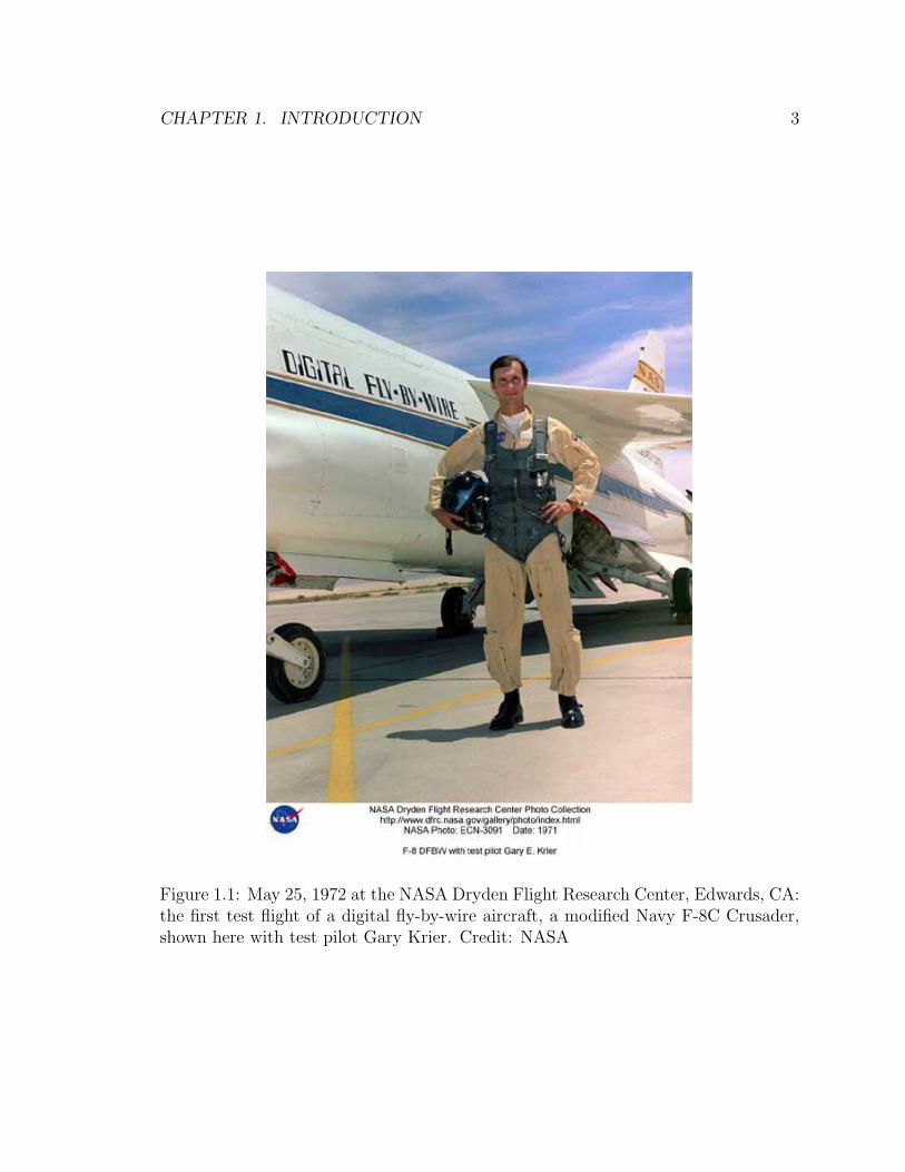
1.1 May 25, 1972 at the NASA Dryden Flight Research Center, Edwards,
CA: the first test flight of a digital fly-by-wire aircraft, a modified Navy
F-8C Crusader, shown here with test pilot Gary Krier. Credit: NASA 3
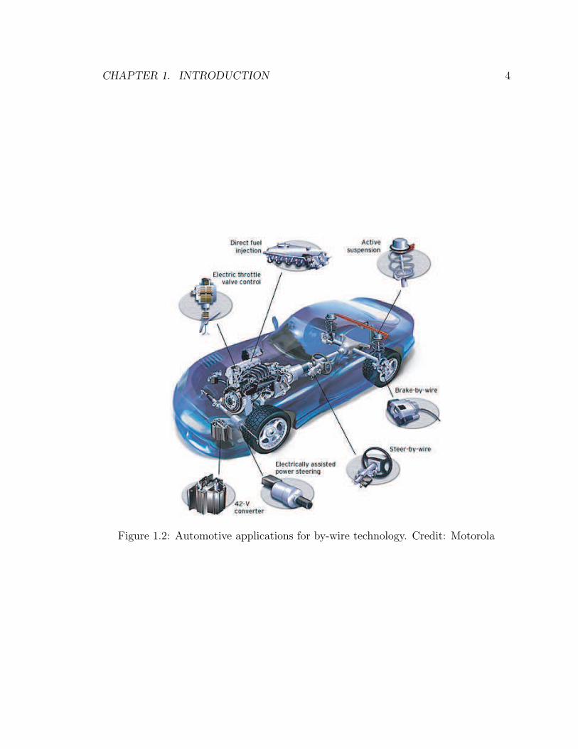
1.2 Automotive applications for by-wire technology. Credit: Motorola . . 4
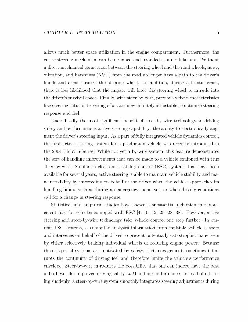
1.3 Yaw moment generated by differential braking (left) versus active steer-
ing (right). . . . . . . . . . . . . . . . . . . . . . . . . . . . . . . . . . 6
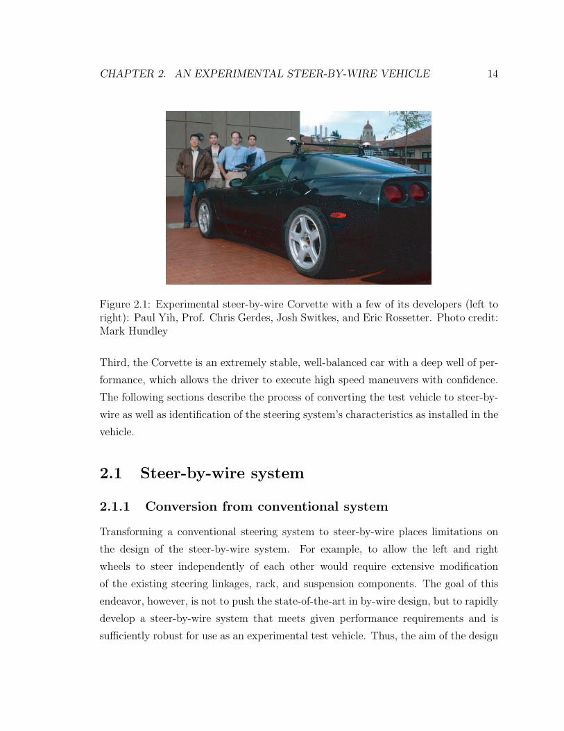
2.1 Experimental steer-by-wire Corvette with a few of its developers (left to
right): Paul Yih, Prof. Chris Gerdes, Josh Switkes, and Eric Rossetter.
Photo credit: Mark Hundley . . . . . . . . . . . . . . . . . . . . . . . 14
2.2 Conventional steering system. . . . . . . . . . . . . . . . . . . . . . . 15
2.3 Conventional steering system converted to steer-by-wire. . . . . . . . 16
2.4 Universal joint. . . . . . . . . . . . . . . . . . . . . . . . . . . . . . . 16
2.5 View of left side of engine compartment showing steer-by-wire system
servomotor actuator (encased in heat shielding). . . . . . . . . . . . . 17
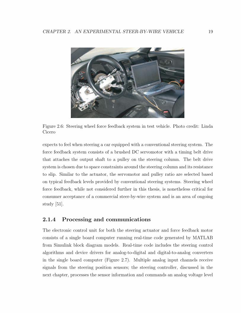
2.6 Steering wheel force feedback system in test vehicle. Photo credit:
Linda Cicero . . . . . . . . . . . . . . . . . . . . . . . . . . . . . . . . 19
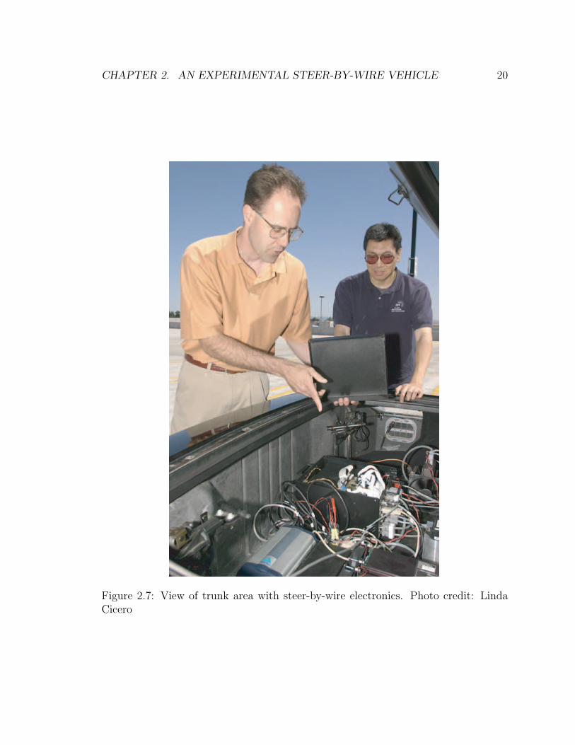
2.7 View of trunk area with steer-by-wire electronics. Photo credit: Linda
Cicero . . . . . . . . . . . . . . . . . . . . . . . . . . . . . . . . . . . 20
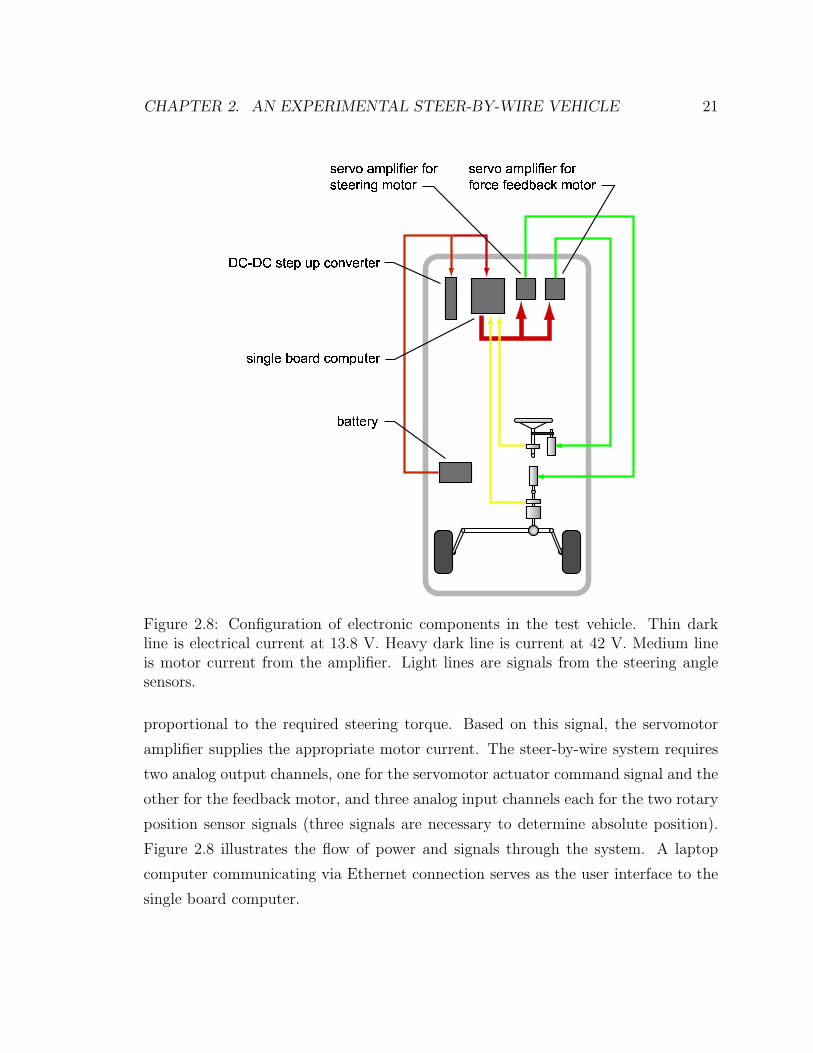
2.8 Configuration of electronic components in the test vehicle. Thin dark
line is electrical current at 13.8 V. Heavy dark line is current at 42
V. Medium line is motor current from the amplifier. Light lines are
signals from the steering angle sensors. . . . . . . . . . . . . . . . . . 21
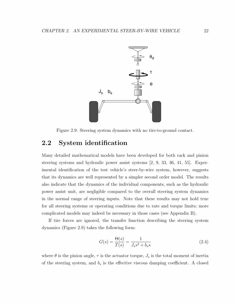
2.9 Steering system dynamics with no tire-to-ground contact. . . . . . . . 22
xiii
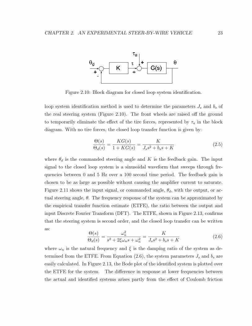
2.10 Block diagram for closed loop system identification. . . . . . . . . . . 23
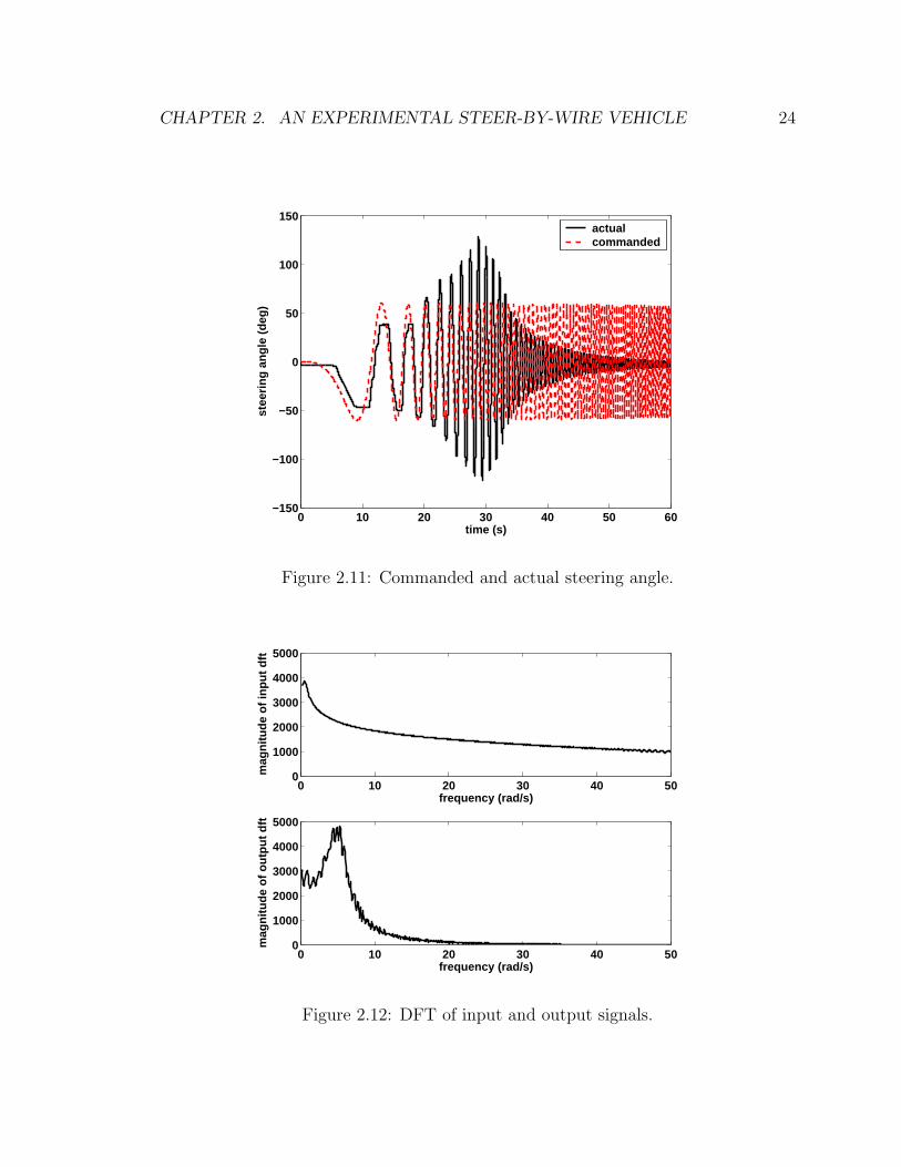
2.11 Commanded and actual steering angle. . . . . . . . . . . . . . . . . . 24
2.12 DFT of input and output signals. . . . . . . . . . . . . . . . . . . . . 24
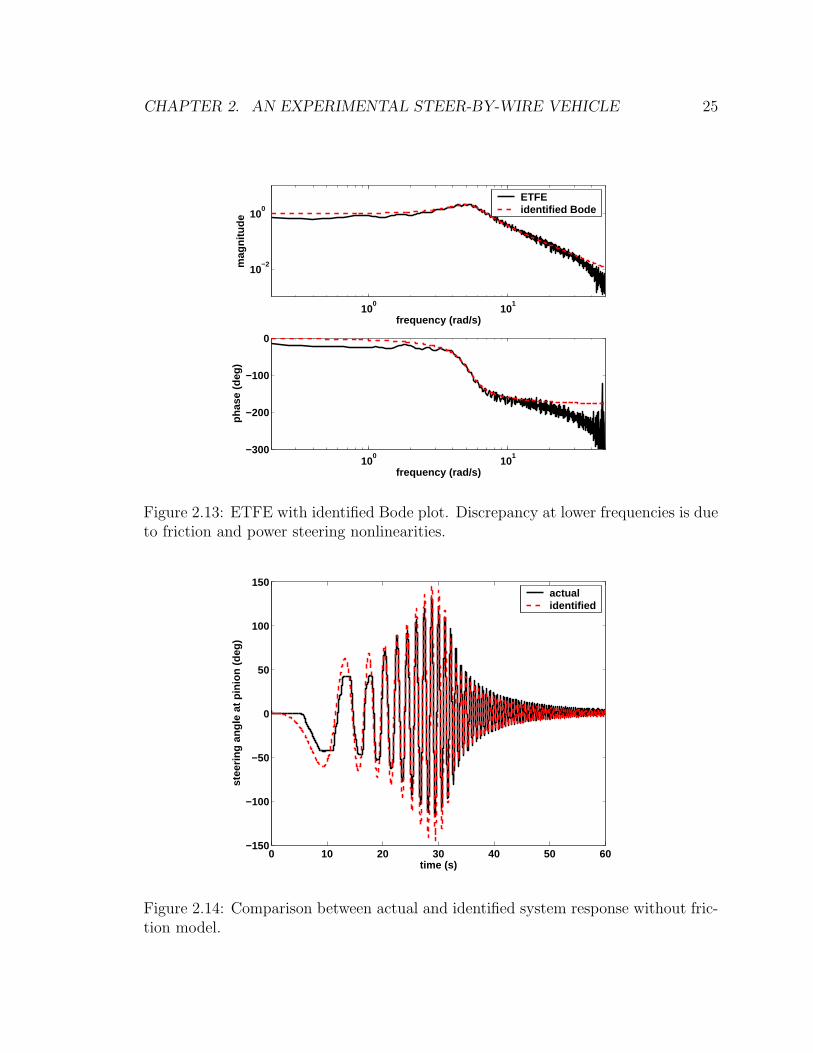
2.13 ETFE with identified Bode plot. Discrepancy at lower frequencies is
due to friction and power steering nonlinearities. . . . . . . . . . . . . 25
2.14 Comparison between actual and identified system response without
friction model. . . . . . . . . . . . . . . . . . . . . . . . . . . . . . . . 25
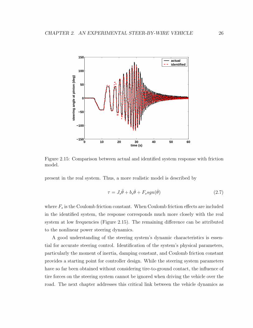
2.15 Comparison between actual and identified system response with fric-
tion model. . . . . . . . . . . . . . . . . . . . . . . . . . . . . . . . . 26
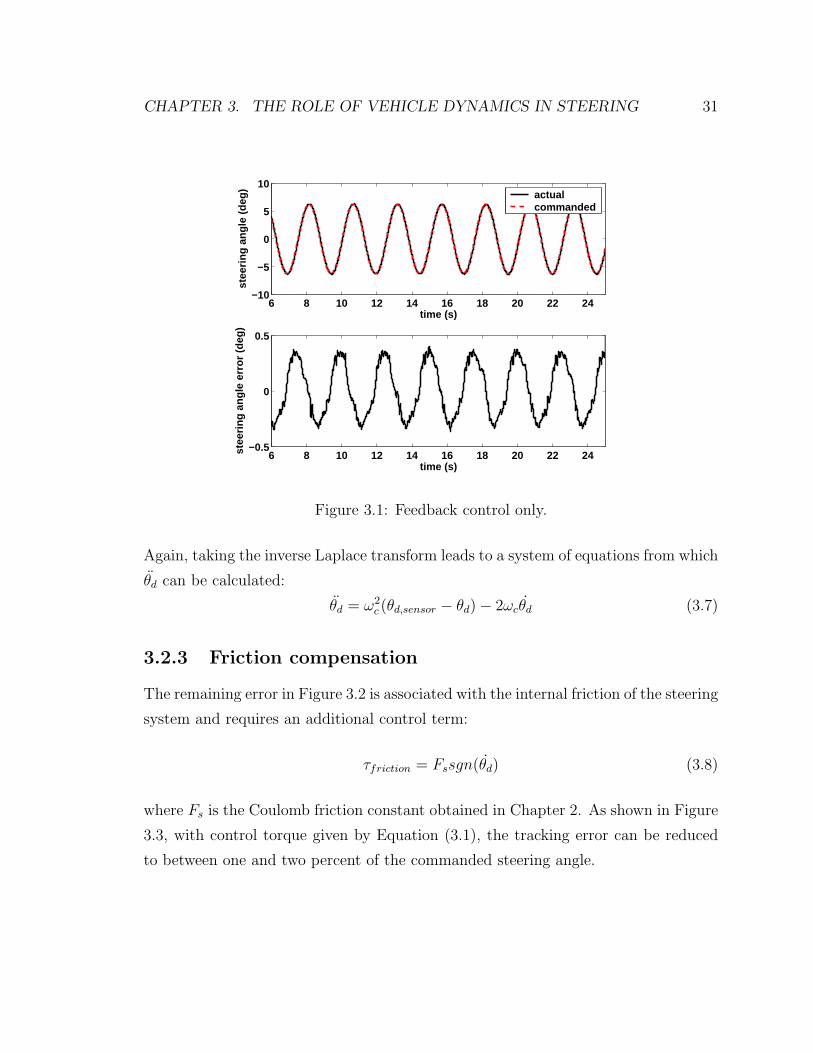
3.1 Feedback control only. . . . . . . . . . . . . . . . . . . . . . . . . . . 31
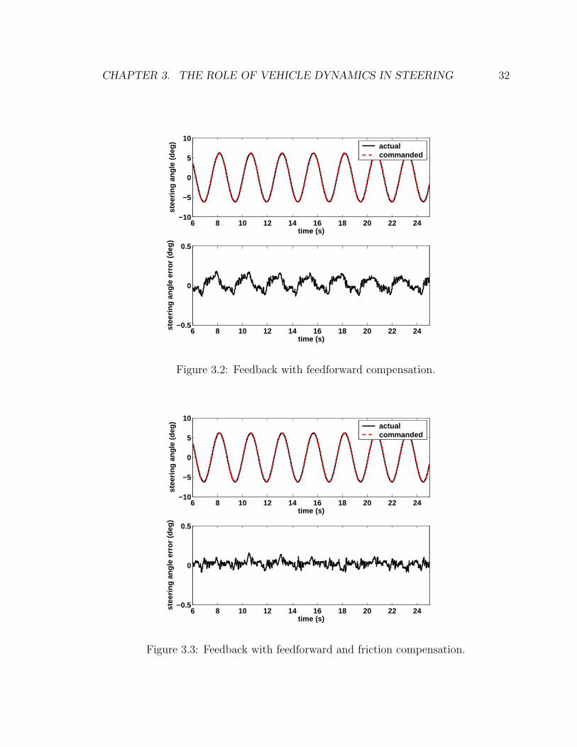
3.2 Feedback with feedforward compensation. . . . . . . . . . . . . . . . 32
3.3 Feedback with feedforward and friction compensation. . . . . . . . . . 32
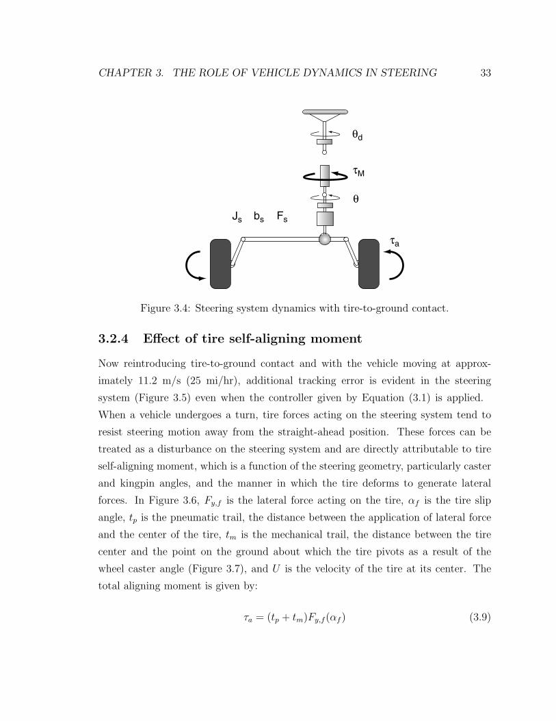
3.4 Steering system dynamics with tire-to-ground contact. . . . . . . . . 33
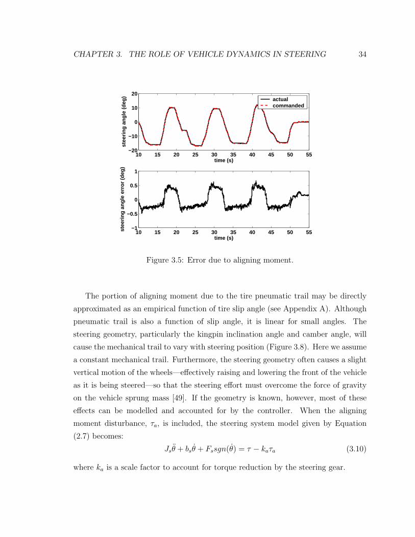
3.5 Error due to aligning moment. . . . . . . . . . . . . . . . . . . . . . . 34
3.6 Tire operating at a slip angle. . . . . . . . . . . . . . . . . . . . . . . 35
3.7 Component of aligning moment due to mechanical trail. . . . . . . . . 35
3.8 Wheel camber and kingpin inclination angle. . . . . . . . . . . . . . . 36
3.9 Steering controller with aligning moment compensation. . . . . . . . . 37
3.10 Steering controller block diagram. . . . . . . . . . . . . . . . . . . . . 38
4.1 NASA’s F6F-3 Hellcat variable stability airplane circa 1950 at the
Ames Aeronautical Laboratory, Moffett Field, California with flight
personnel. Note the vane on the wingtip for measuring aircraft sideslip
angle. Credit: NASA . . . . . . . . . . . . . . . . . . . . . . . . . . . 41
4.2 Front views of aircraft showing (a) positive dihedral, (b) sideslip due
to bank angle, and (c) stabilizing roll moment. Credit: NASA . . . . 42
4.3 Bicycle model. . . . . . . . . . . . . . . . . . . . . . . . . . . . . . . . 44
4.4 The fundamental handling characteristics as determined by the sign of
the understeer gradient. . . . . . . . . . . . . . . . . . . . . . . . . . 46
4.5 Steady state cornering. . . . . . . . . . . . . . . . . . . . . . . . . . . 47
xiv
4.6 Nonlinear vehicle simulation with and without handling modification:
neutral steering case. . . . . . . . . . . . . . . . . . . . . . . . . . . . 52
4.7 Nonlinear vehicle simulation with and without handling modification:
oversteering case. . . . . . . . . . . . . . . . . . . . . . . . . . . . . . 52
4.8 Sideslip and yaw rate estimation. . . . . . . . . . . . . . . . . . . . . 53
4.9 Steer-by-wire Corvette undergoing testing on the West Parallel of Mof-
fett Federal Airfield at the NASA Ames Research Center. Moffett is
an active airfield. . . . . . . . . . . . . . . . . . . . . . . . . . . . . . 54
4.10 Comparison between yaw rate of bicycle model and experiment with
normal cornering stiffness. . . . . . . . . . . . . . . . . . . . . . . . . 55
4.11 Comparison between sideslip angle of bicycle model and experiment
with normal cornering stiffness. . . . . . . . . . . . . . . . . . . . . . 56
4.12 Difference in road wheel angle with effectively reduced front cornering
stiffness. . . . . . . . . . . . . . . . . . . . . . . . . . . . . . . . . . . 57
4.13 Comparison between yaw rate of normal and effectively reduced front
cornering stiffness. . . . . . . . . . . . . . . . . . . . . . . . . . . . . 57
4.14 Comparison between lateral acceleration of normal and effectively re-
duced front cornering stiffness. . . . . . . . . . . . . . . . . . . . . . . 58
4.15 Comparison between yaw rate of bicycle model and experiment with
reduced front cornering stiffness. . . . . . . . . . . . . . . . . . . . . . 58
4.16 Comparison between sideslip angle of bicycle model and experiment
with reduced front cornering stiffness. . . . . . . . . . . . . . . . . . . 59
4.17 Difference in road wheel angle with effectively increased front cornering
stiffness. . . . . . . . . . . . . . . . . . . . . . . . . . . . . . . . . . . 59
4.18 Comparison between yaw rate of normal and effectively increased front
cornering stiffness. . . . . . . . . . . . . . . . . . . . . . . . . . . . . 60
4.19 Comparison between lateral acceleration of normal and effectively in-
creased front cornering stiffness. . . . . . . . . . . . . . . . . . . . . . 60
4.20 Comparison between yaw rate of bicycle model and experiment with
increased front cornering stiffness. . . . . . . . . . . . . . . . . . . . . 61
xv
4.21 Comparison between sideslip angle of bicycle model and experiment
with increased front cornering stiffness. . . . . . . . . . . . . . . . . . 61
4.22 Comparison between yaw rate of unloaded and loaded vehicle. . . . . 62
4.23 Comparison between yaw rate of unloaded vehicle and loaded vehicle
with handling modification. . . . . . . . . . . . . . . . . . . . . . . . 63
5.1 Steering system dynamics. . . . . . . . . . . . . . . . . . . . . . . . . 67
5.2 Conventional observer block diagram. . . . . . . . . . . . . . . . . . . 72
5.3 Cascaded observer block diagram. . . . . . . . . . . . . . . . . . . . . 74
5.4 Estimated steer angle from conventional observer. . . . . . . . . . . . 80
5.5 Estimated steer rate from conventional observer. . . . . . . . . . . . . 80
5.6 Estimated sideslip from conventional observer. . . . . . . . . . . . . . 81
5.7 Estimated yaw rate from conventional observer. . . . . . . . . . . . . 81
5.8 Estimated steer angle from disturbance observer. . . . . . . . . . . . 82
5.9 Estimated steer rate from disturbance observer. . . . . . . . . . . . . 82
5.10 Estimated sideslip from disturbance observer. . . . . . . . . . . . . . 83
5.11 Estimated yaw rate from disturbance observer. . . . . . . . . . . . . . 83
5.12 Estimated disturbance torque. . . . . . . . . . . . . . . . . . . . . . . 84
5.13 Estimated disturbance torque versus slip angle. . . . . . . . . . . . . 85
5.14 Comparison between estimated yaw rate, INS measurement, and bicy-
cle model simulation with normal cornering stiffness. . . . . . . . . . 88
5.15 Comparison between estimated sideslip angle, GPS measurement, and
bicycle model simulation with normal cornering stiffness. . . . . . . . 88
5.16 Difference in road wheel angle with effectively reduced front cornering
stiffness. . . . . . . . . . . . . . . . . . . . . . . . . . . . . . . . . . . 89
5.17 Comparison between lateral acceleration with normal and effectively
reduced front cornering stiffness. . . . . . . . . . . . . . . . . . . . . . 90
5.18 Comparison between estimated yaw rate, INS measurement, and bicy-
cle model simulation with reduced front cornering stiffness. . . . . . . 90
5.19 Comparison between estimated sideslip angle, GPS measurement, and
bicycle model simulation with reduced front cornering stiffness. . . . . 91
xvi
5.20 Difference in road wheel angle with effectively increased front cornering
stiffness. . . . . . . . . . . . . . . . . . . . . . . . . . . . . . . . . . . 91
5.21 Comparison between lateral acceleration with normal and effectively
increased front cornering stiffness. . . . . . . . . . . . . . . . . . . . . 92
5.22 Comparison between estimated yaw rate, INS measurement, and bicy-
cle model simulation with increased front cornering stiffness. . . . . . 92
5.23 Comparison between estimated sideslip angle, GPS measurement, and
bicycle model simulation with increased front cornering stiffness. . . . 93
6.1 Tire cornering stiffness in the nonlinear region represented by Cα,NL. 98
6.2 Next generation experimental drive-by-wire vehicle. . . . . . . . . . . 100
A.1 Tire operating at a slip angle. . . . . . . . . . . . . . . . . . . . . . . 101
A.2 Tire lateral force versus slip angle. . . . . . . . . . . . . . . . . . . . . 104
A.3 Slip angle versus component of aligning moment due to pneumatic trail.104
B.1 Hydraulic power assist schematic. . . . . . . . . . . . . . . . . . . . . 107
B.2 Mechanical representation of steering system with hydraulic power assist.109
B.3 Orifice area versus valve angle. . . . . . . . . . . . . . . . . . . . . . . 111
B.4 Typical power steering boost curve: assist pressure versus input torque
with linear approximation. . . . . . . . . . . . . . . . . . . . . . . . . 111
C.1 Bicycle model with front and rear steering. . . . . . . . . . . . . . . . 113
xvii
Chapter 1
Introduction
1.1 Evolution of automotive steering systems
The proliferation of electronic control systems is nowhere more apparent than in the
modern automobile. During the last two decades, advances in electronics have revo-
lutionized many aspects of automotive engineering, especially in the areas of engine
combustion management and vehicle safety systems such as anti-lock brakes (ABS)
and electronic stability control (ESC). The benefits of applying electronic technology
are clear: improved performance, safety, and reliability with reduced manufacturing
and operating costs. However, only recently has the electronic revolution begun to
find its way into automotive steering systems in the form of electronically controlled
variable assist and, within the past two years, fully electric power assist [5, 40].
The basic design of automotive steering systems has changed little since the in-
vention of the steering wheel: the driver’s steering input is transmitted by a shaft
through some type of gear reduction mechanism (most commonly rack and pinion or
recirculating ball bearings) to generate steering motion at the front wheels. One of
the more prominent developments in the history of the automobile occurred in the
1950s when hydraulic power steering assist was first introduced. Since then, power
assist has become a standard component in modern automotive steering systems. Us-
ing hydraulic pressure supplied by an engine-driven pump, power steering amplifies
and supplements the driver-applied torque at the steering wheel so that steering effort
1
CHAPTER 1. INTRODUCTION 2
is reduced. In addition to improved comfort, reducing steering effort has important
safety implications as well, such as allowing a driver to more easily swerve to avoid
an accident.
The recent introduction of electric power steering in production vehicles elimi-
nates the need for the hydraulic pump. Electric power steering is more efficient than
conventional power steering, since the electric power steering motor only needs to pro-
vide assist when the steering wheel is turned, whereas the hydraulic pump must run
constantly. The assist level is also easily tunable to the vehicle type, road speed, and
even driver preference [32, 6]. An added benefit is the elimination of environmental
hazard posed by leakage and disposal of hydraulic power steering fluid.
The next step in steering system evolution—to completely do away with the steer-
ing column and shaft—represents a dramatic departure from traditional automotive
design practice. The substitution of electronic systems in place of mechanical or hy-
draulic controls is known as by-wire technology. This idea is certainly not new to
airplane pilots [46]; many modern aircraft, both commercial and military, rely com-
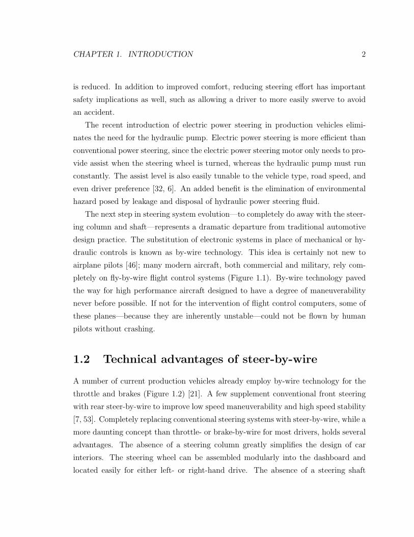
pletely on fly-by-wire flight control systems (Figure 1.1). By-wire technology paved
the way for high performance aircraft designed to have a degree of maneuverability
never before possible. If not for the intervention of flight control computers, some of
these planes—because they are inherently unstable—could not be flown by human
pilots without crashing.
1.2 Technical advantages of steer-by-wire
A number of current production vehicles already employ by-wire technology for the
throttle and brakes (Figure 1.2) [21]. A few supplement conventional front steering
with rear steer-by-wire to improve low speed maneuverability and high speed stability
[7, 53]. Completely replacing conventional steering systems with steer-by-wire, while a
more daunting concept than throttle- or brake-by-wire for most drivers, holds several
advantages. The absence of a steering column greatly simplifies the design of car
interiors. The steering wheel can be assembled modularly into the dashboard and
located easily for either left- or right-hand drive. The absence of a steering shaft
CHAPTER 1. INTRODUCTION 3
Figure 1.1: May 25, 1972 at the NASA Dryden Flight Research Center, Edwards, CA:the first test flight of a digital fly-by-wire aircraft, a modified Navy F-8C Crusader,shown here with test pilot Gary Krier. Credit: NASA
CHAPTER 1. INTRODUCTION 4
Figure 1.2: Automotive applications for by-wire technology. Credit: Motorola
CHAPTER 1. INTRODUCTION 5
allows much better space utilization in the engine compartment. Furthermore, the
entire steering mechanism can be designed and installed as a modular unit. Without
a direct mechanical connection between the steering wheel and the road wheels, noise,
vibration, and harshness (NVH) from the road no longer have a path to the driver’s
hands and arms through the steering wheel. In addition, during a frontal crash,
there is less likelihood that the impact will force the steering wheel to intrude into
the driver’s survival space. Finally, with steer-by-wire, previously fixed characteristics
like steering ratio and steering effort are now infinitely adjustable to optimize steering
response and feel.
Undoubtedly the most significant benefit of steer-by-wire technology to driving
safety and performance is active steering capability: the ability to electronically aug-
ment the driver’s steering input. As a part of fully integrated vehicle dynamics control,
the first active steering system for a production vehicle was recently introduced in
the 2004 BMW 5-Series. While not yet a by-wire system, this feature demonstrates
the sort of handling improvements that can be made to a vehicle equipped with true
steer-by-wire. Similar to electronic stability control (ESC) systems that have been
available for several years, active steering is able to maintain vehicle stability and ma-
neuverability by interceding on behalf of the driver when the vehicle approaches its
handling limits, such as during an emergency maneuver, or when driving conditions
call for a change in steering response.
Statistical and empirical studies have shown a substantial reduction in the ac-
cident rate for vehicles equipped with ESC [4, 10, 12, 25, 28, 38]. However, active
steering and steer-by-wire technology take vehicle control one step further. In cur-
rent ESC systems, a computer analyzes information from multiple vehicle sensors
and intervenes on behalf of the driver to prevent potentially catastrophic maneuvers
by either selectively braking individual wheels or reducing engine power. Because
these types of systems are motivated by safety, their engagement sometimes inter-
rupts the continuity of driving feel and therefore limits the vehicle’s performance
envelope. Steer-by-wire introduces the possibility that one can indeed have the best
of both worlds: improved driving safety and handling performance. Instead of intrud-
ing suddenly, a steer-by-wire system smoothly integrates steering adjustments during
CHAPTER 1. INTRODUCTION 6
Fx
Fy Fy
t/2
a
Figure 1.3: Yaw moment generated by differential braking (left) versus active steering(right).
an emergency maneuver to maintain stability [7]. The benefits go beyond stability
control: for example, a large, heavy vehicle can be made to feel as responsive as a
smaller, lighter vehicle during normal driving. The ability to actively steer the front
wheels allows artificial tuning of a vehicle’s handling characteristics to suit the driver’s
preference.
Furthermore, in some cases it is actually advantageous to utilize steering instead
of differential braking to generate yaw moment, because steering requires less friction
force between the tires and ground. Consider the case when the rear tires have reached
their limits of adhesion during cornering, e.g. a rear wheel slide; the only means of
control are the front wheels. This situation typically leads to a spinout or, with
poorly timed steering inputs, a violent fishtailing that is nearly impossible to control.
To generate a correcting yaw moment, one can either apply braking to the outside
front wheel or counter steer the front wheels (Figure 1.3). The moment generated by
differential braking is:
M = Fx
t
2(1.1)
CHAPTER 1. INTRODUCTION 7
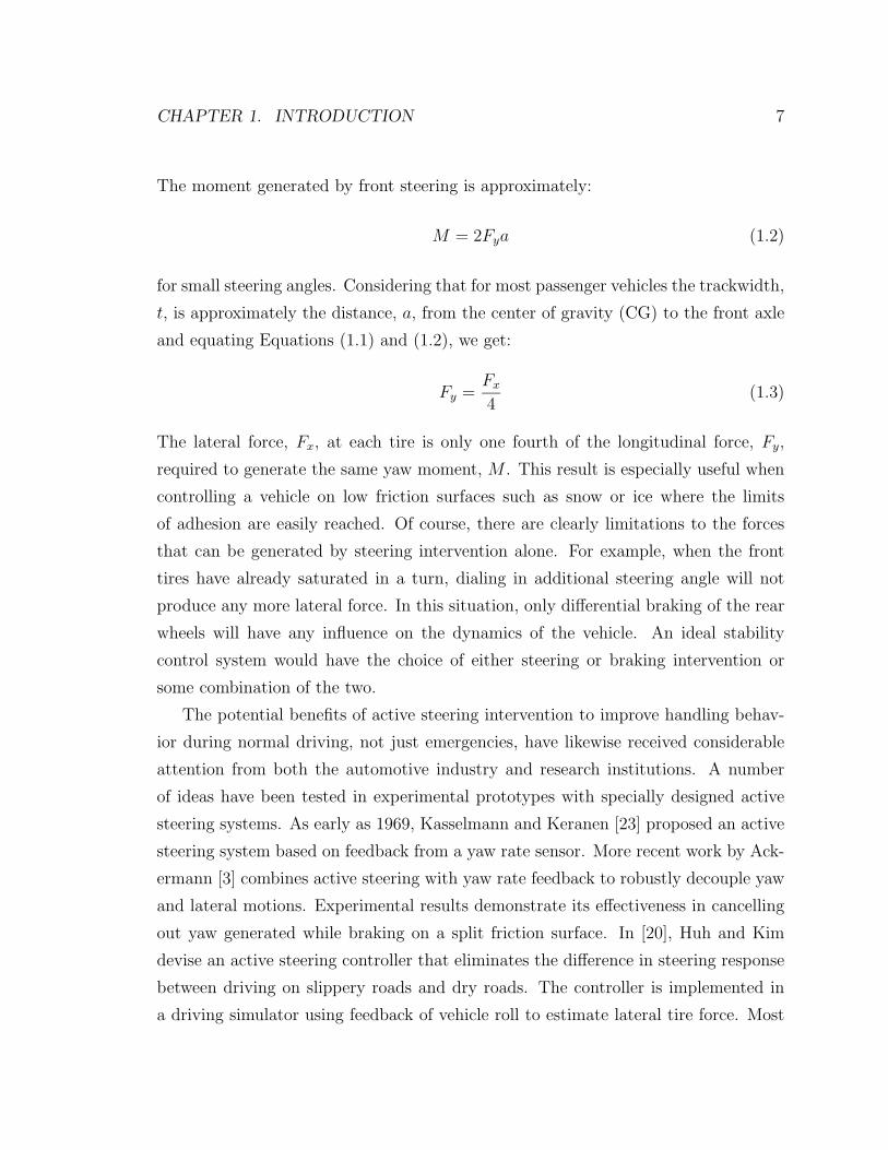
The moment generated by front steering is approximately:
M = 2Fya (1.2)
for small steering angles. Considering that for most passenger vehicles the trackwidth,
t, is approximately the distance, a, from the center of gravity (CG) to the front axle
and equating Equations (1.1) and (1.2), we get:
Fy =Fx
4(1.3)
The lateral force, Fx, at each tire is only one fourth of the longitudinal force, Fy,
required to generate the same yaw moment, M . This result is especially useful when
controlling a vehicle on low friction surfaces such as snow or ice where the limits
of adhesion are easily reached. Of course, there are clearly limitations to the forces
that can be generated by steering intervention alone. For example, when the front
tires have already saturated in a turn, dialing in additional steering angle will not
produce any more lateral force. In this situation, only differential braking of the rear
wheels will have any influence on the dynamics of the vehicle. An ideal stability
control system would have the choice of either steering or braking intervention or
some combination of the two.
The potential benefits of active steering intervention to improve handling behav-
ior during normal driving, not just emergencies, have likewise received considerable
attention from both the automotive industry and research institutions. A number
of ideas have been tested in experimental prototypes with specially designed active
steering systems. As early as 1969, Kasselmann and Keranen [23] proposed an active
steering system based on feedback from a yaw rate sensor. More recent work by Ack-
ermann [3] combines active steering with yaw rate feedback to robustly decouple yaw
and lateral motions. Experimental results demonstrate its effectiveness in cancelling
out yaw generated while braking on a split friction surface. In [20], Huh and Kim
devise an active steering controller that eliminates the difference in steering response
between driving on slippery roads and dry roads. The controller is implemented in
a driving simulator using feedback of vehicle roll to estimate lateral tire force. Most
CHAPTER 1. INTRODUCTION 8
recently, Segawa et al. [48] apply lateral acceleration and yaw rate feedback to an
experimental steer-by-wire vehicle and demonstrate that active steering control can
achieve greater driving stability than differential brake control.
1.3 An increasing need for sensing and estimation
While most of the previously implemented active steering systems rely on feedback
of yaw rate or lateral acceleration or a combination of both, since these signals are
readily measured with inexpensive sensors, significantly more comprehensive control
can be achieved given information on vehicle sideslip angle. Sideslip is defined as
the difference between the vehicle’s forward orientation and its direction of velocity.
The advantages of knowing sideslip are twofold: first, yaw rate and sideslip together
completely describe a vehicle’s motion in the road plane. Yaw rate alone is not always
enough; for example, a vehicle could be undergoing an acceptable yaw rate, but it
might be skidding sideways. The second reason for obtaining sideslip information is
that the driver is particularly sensitive to sideslip motion of the vehicle and prefers
the angle to be small [11]. This preference arises from the sensation of instability at
larger angles which is perhaps rooted in the real potential for loss of control when
sideslip angle and therefore tire slip angles are allowed to grow to large.
Although feedback of sideslip angle has been proposed theoretically [17, 34, 27, 35],
the difficulty in estimating vehicle sideslip presents an obstacle to achieving sideslip
control. Stability systems currently available on production cars typically derive slip
rate from accelerometer integration, a physical vehicle model, or a combination of
the two, but these estimation methods are prone to uncertainty [54]. For example,
direct integration of lateral acceleration can accumulate sensor errors and unwanted
measurements from road grade and bank angle. Because sideslip is extremely impor-
tant to the driver’s perception of handling behavior, quality of the driving experience
depends strongly on quality of the feedback signal. This dependence is less critical
for stability control systems, which tend to engage when the vehicle is already under-
going extreme maneuvers, but to improve handling behavior during normal driving
requires cleaner and more accurate feedback.
CHAPTER 1. INTRODUCTION 9
An estimation scheme that overcomes some of these drawbacks supplements in-
tegration of inertial sensors with Global Positioning System (GPS) measurements
[44]. Absolute GPS heading and velocity measurements eliminate the errors from
inertial navigation system (INS) integration; conversely, INS sensors complement the
GPS measurements by providing higher update rate estimates of the vehicle states.
However, during periods of GPS signal loss, which frequently occur in urban driving
environments, integration errors can still accumulate and lead to faulty estimates.
The growing presence of electric power steering systems in production vehicles
introduces yet another absolute measurement—steering torque—from which vehicle
sideslip angle may be estimated. Through the tire self-aligning moment, which com-
prises much of the resistance felt by the driver when turning the steering wheel,
steering torque is directly related to the lateral front tire forces, which in turn relate
to the tire slip angles and therefore the vehicle states. This approach is especially
suited to vehicles equipped with steer-by-wire since the steering torque can easily
be determined from the current applied to the steering motor. As such, steer-by-
wire encompasses the entire scope of vehicle dynamics control: on the one hand, the
steer-by-wire system is the actuator that provides control authority for the vehicle
dynamics controller. On the other hand, it is the sensor from which the vehicle states
are estimated.
1.4 Thesis contributions
The contributions of this dissertation are as follows:
• A general approach for steering control using a steer-by-wire system. The com-
bined feedback and feedfoward control strategy systematically cancels out the
steering system dynamics, friction, and disturbance forces. In doing so, it es-
tablishes the need to compensate for the aligning moment effect on steering.
• The application of active steering and full vehicle state feedback to modify a
vehicle’s handling characteristics. By augmenting the driver’s steering input,
CHAPTER 1. INTRODUCTION 10
the effect is equivalent to changing the front tire cornering stiffness and therefore
the balance between handling responsiveness and stability.
• The development and implementation of a vehicle sideslip observer based on
steering torque. The observer combines models of the steering system dynamics
and vehicle dynamics in the way they are naturally linked through the tire forces.
• A springboard for critical research issues facing steer-by-wire technology, par-
ticularly by-wire diagnostics. A thorough understanding of steering system and
vehicle dynamics and how to measure or estimate the key parameters form the
elements of a comprehensive model-based diagnostic approach.
1.5 Thesis overview
The potential for improved driving safety and handling performance afforded by steer-
by-wire capability deserves thorough study. There is no greater validation of a promis-
ing technology than to physically demonstrate its effectiveness in a real-world envi-
ronment. Chapter 2 discusses the conversion of a conventional passenger car into a
steer-by-wire prototype vehicle. It also describes a closed loop experimental method
for identification of the steering system dynamics, since precise control of the steer-
by-wire system depends on accurate knowledge of the steering system parameters.
The ability to precisely control the steering angle of the steer-by-wire system is
crucial for both direct steering and active steering control. In other words, the steer
angles at the road wheels must be as close as possible to the angles commanded by
either the driver or the control system. Chapter 3 develops a proportional derivative
controller with feedforward of steering rate and acceleration in order to cancel out the
steering system dynamics. Particularly, this chapter emphasizes the importance of
the vehicle dynamics forces as they are transmitted through the tire aligning moment
to act on the steering system. Precise control cannot be achieved without accounting
for these external forces.
There are certainly many ways in which active steering intervention can be applied
to improve handling performance and safety. Chapter 4 presents a physically intuitive
CHAPTER 1. INTRODUCTION 11
application based on feedback of the vehicle states, yaw rate and sideslip angle. The
effect is exactly equivalent to changing the cornering stiffness of the front tires. This
“virtual tire change” results in a modification of the fundamental handling character-
istics of the vehicle, i.e. from neutral steering to oversteering or understeering. Even
though neutral steering is the ideal handling characteristic since it provides maximum
steering response without instability, passenger vehicles are typically designed to be
inherently understeering in order to avoid the possibility of unstable behavior when
operating conditions—such as load distribution or disproportionate tire wear—cause
an undesirable shift in handling characteristics. This design compromise necessarily
reduces the responsiveness of the vehicle so that it is not as responsive as it could be
in all situations. It is not possible to physically design a vehicle that handles opti-
mally under every condition; however, with a combination of active steering and full
state feedback control, optimal handling characteristics are achievable even though
a vehicle’s physical parameters may be suboptimal. Thus, such a vehicle’s handling
characteristics can be arbitrarily tuned to driver preference as well as to maintain
consistent behavior when operating conditions vary. Active handling modification is
demonstrated on the test vehicle using sideslip estimates from a GPS/INS system
installed in the test vehicle.
The downside to relying on GPS for sideslip is that the GPS signal can be lost, par-
ticularly in urban environments. Fortuitously, steer-by-wire provides a ready solution
to the problem of sideslip estimation. Chapter 5 presents an alternative approach to
estimating the vehicle sideslip using steering torque information. A complete knowl-
edge of steering torque can be determined from the current applied to the system’s
steering actuator. Through the tire self-aligning moment, steering torque can be
directly related to the front tire lateral forces and therefore the wheel slip angles.
Chapter 5 develops two observer structures based on linear models of the vehicle and
tire behavior to estimate the vehicle states from measurements of steering angle and
yaw rate. The first of the two structures combines the vehicle and steering system
models into a single observer structure to estimate four states at once: sideslip an-
gle, yaw rate, steering angle, and steering rate. The second structure incorporates
an intermediate step. A disturbance observer based on the steering system model
CHAPTER 1. INTRODUCTION 12
estimates the tire aligning moment; this estimate becomes the measurement part of
a vehicle state observer for sideslip and yaw rate. The handling modification experi-
ments are repeated using this method of sideslip estimation in place of GPS/INS. For
the tests performed, the sideslip estimation results are comparable to those obtained
from the GPS/INS method. However, the results also suggest that in order to more
effectively use the aligning moment for lateral force measurement, some changes to the
original steer-by-wire system design are necessary. The future work section (Chapter
6) discusses some of the changes that are being implemented in the next generation
of experimental by-wire vehicles.
Chapter 2
An experimental steer-by-wire
vehicle
Although a number of automotive companies have developed their own steer-by-wire
prototypes, very few examples of such vehicles exist at academic institutions. Most
academic studies related to steer-by-wire have been theoretical and validated only in
simulation [31, 59, 60, 18, 52] mainly due to the cost and complexity of acquiring
a vehicle and converting it to steer-by-wire. The author’s interest in steer-by-wire
began as an effort to help experimentally verify promising research in lane-keeping
assistance systems [43]. The desire for a relatively simple and robust system dictated
the process of transforming a stock 1997 Chevrolet Corvette into a rolling testbed
with steer-by-wire capability. Out of this endeavor emerged several new research
directions, some of which are developed in the succeeding chapters.
The test vehicle, generously donated by General Motors Corporation, is a regular
production model two-door coupe with a four-speed overdrive automatic transmis-
sion. Three factors make this vehicle ideal for experimental testing. First, the layout
of the vehicle— front-engine, longitudinally mounted V-8, and open trunk area—
facilitates the locating of test equipment and routing of electrical wiring. Second, the
vehicle is designed and engineered with serviceability in mind, which means critical
components are reasonably accessible and installation of experimental apparatus can
be completed in a timely manner with minimal modification to the existing structure.
13
CHAPTER 2. AN EXPERIMENTAL STEER-BY-WIRE VEHICLE 14
Figure 2.1: Experimental steer-by-wire Corvette with a few of its developers (left toright): Paul Yih, Prof. Chris Gerdes, Josh Switkes, and Eric Rossetter. Photo credit:Mark Hundley
Third, the Corvette is an extremely stable, well-balanced car with a deep well of per-
formance, which allows the driver to execute high speed maneuvers with confidence.
The following sections describe the process of converting the test vehicle to steer-by-
wire as well as identification of the steering system’s characteristics as installed in the
vehicle.
2.1 Steer-by-wire system
2.1.1 Conversion from conventional system
Transforming a conventional steering system to steer-by-wire places limitations on
the design of the steer-by-wire system. For example, to allow the left and right
wheels to steer independently of each other would require extensive modification
of the existing steering linkages, rack, and suspension components. The goal of this
endeavor, however, is not to push the state-of-the-art in by-wire design, but to rapidly
develop a steer-by-wire system that meets given performance requirements and is
sufficiently robust for use as an experimental test vehicle. Thus, the aim of the design
CHAPTER 2. AN EXPERIMENTAL STEER-BY-WIRE VEHICLE 15
handwheel
universal joints
pinion
rack
gear assembly
steering column
intermediate shaft
power assist unit
Figure 2.2: Conventional steering system.
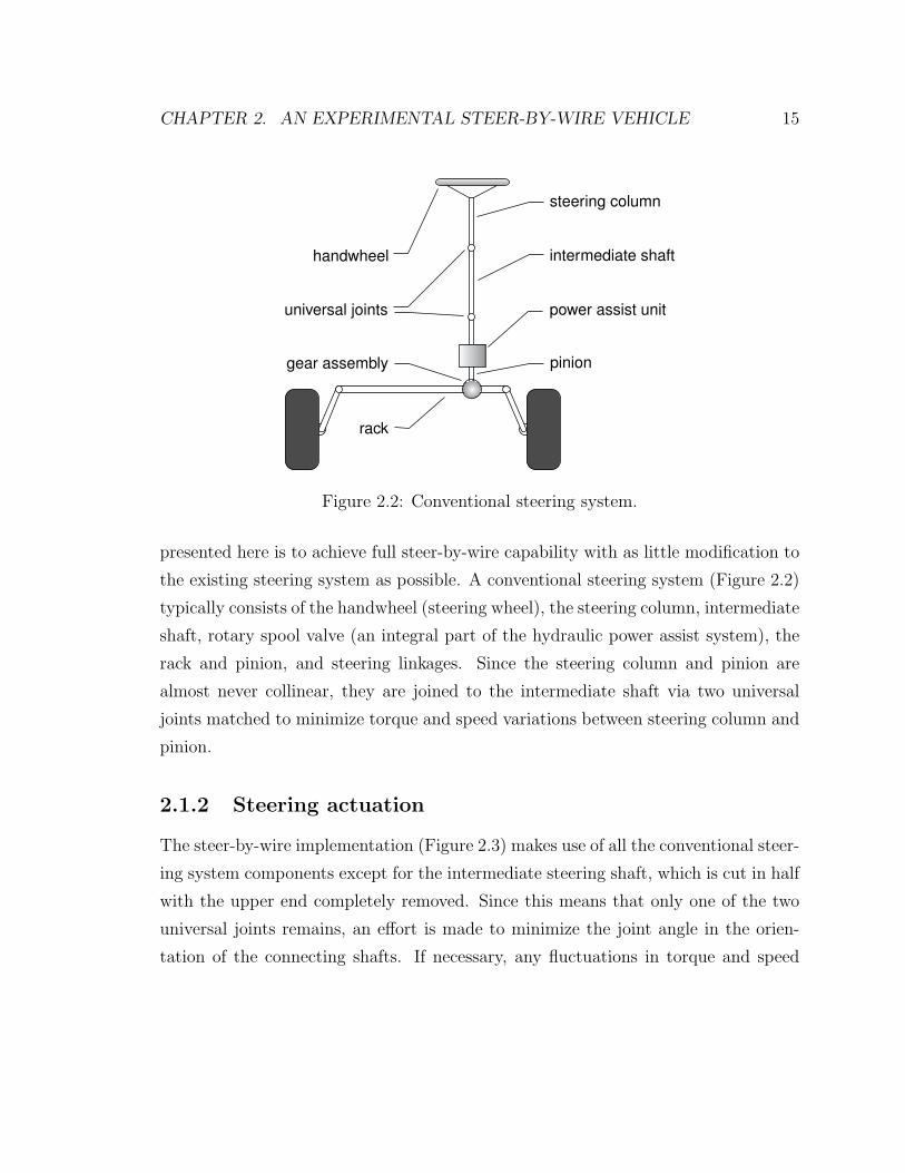
presented here is to achieve full steer-by-wire capability with as little modification to
the existing steering system as possible. A conventional steering system (Figure 2.2)
typically consists of the handwheel (steering wheel), the steering column, intermediate
shaft, rotary spool valve (an integral part of the hydraulic power assist system), the
rack and pinion, and steering linkages. Since the steering column and pinion are
almost never collinear, they are joined to the intermediate shaft via two universal
joints matched to minimize torque and speed variations between steering column and
pinion.
2.1.2 Steering actuation
The steer-by-wire implementation (Figure 2.3) makes use of all the conventional steer-
ing system components except for the intermediate steering shaft, which is cut in half
with the upper end completely removed. Since this means that only one of the two
universal joints remains, an effort is made to minimize the joint angle in the orien-
tation of the connecting shafts. If necessary, any fluctuations in torque and speed
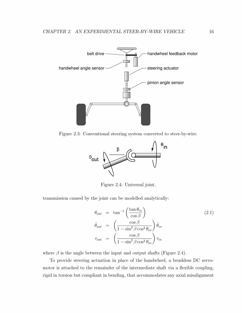
CHAPTER 2. AN EXPERIMENTAL STEER-BY-WIRE VEHICLE 16
belt drive
handwheel angle sensor
handwheel feedback motor
steering actuator
pinion angle sensor
Figure 2.3: Conventional steering system converted to steer-by-wire.
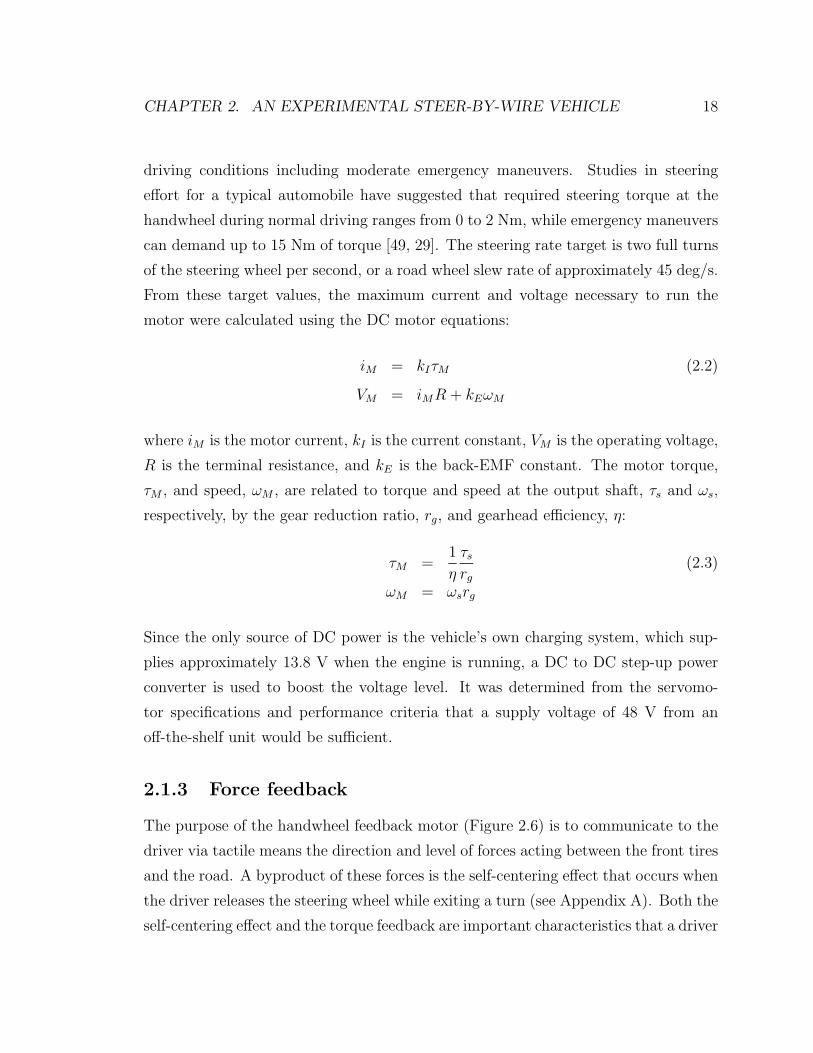
���
����
�
Figure 2.4: Universal joint.
transmission caused by the joint can be modelled analytically:
θout = tan−1
(
tan θin
cos β
)
(2.1)
θout =
(
cos β
1 − sin2 β cos2 θin
)
θin
τout =
(
cos β
1 − sin2 β cos2 θin
)
τin
where β is the angle between the input and output shafts (Figure 2.4).
To provide steering actuation in place of the handwheel, a brushless DC servo-
motor is attached to the remainder of the intermediate shaft via a flexible coupling,
rigid in torsion but compliant in bending, that accommodates any axial misalignment
CHAPTER 2. AN EXPERIMENTAL STEER-BY-WIRE VEHICLE 17
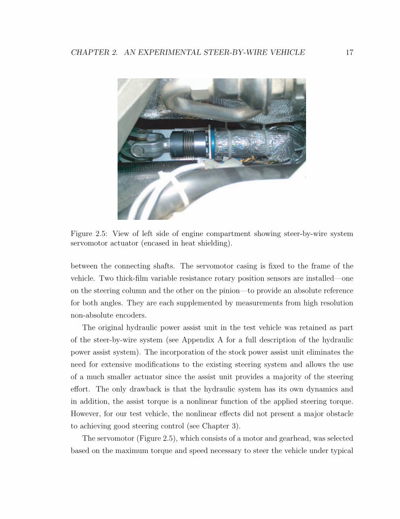
Figure 2.5: View of left side of engine compartment showing steer-by-wire systemservomotor actuator (encased in heat shielding).
between the connecting shafts. The servomotor casing is fixed to the frame of the
vehicle. Two thick-film variable resistance rotary position sensors are installed—one
on the steering column and the other on the pinion—to provide an absolute reference
for both angles. They are each supplemented by measurements from high resolution
non-absolute encoders.
The original hydraulic power assist unit in the test vehicle was retained as part
of the steer-by-wire system (see Appendix A for a full description of the hydraulic
power assist system). The incorporation of the stock power assist unit eliminates the
need for extensive modifications to the existing steering system and allows the use
of a much smaller actuator since the assist unit provides a majority of the steering
effort. The only drawback is that the hydraulic system has its own dynamics and
in addition, the assist torque is a nonlinear function of the applied steering torque.
However, for our test vehicle, the nonlinear effects did not present a major obstacle
to achieving good steering control (see Chapter 3).
The servomotor (Figure 2.5), which consists of a motor and gearhead, was selected
based on the maximum torque and speed necessary to steer the vehicle under typical
CHAPTER 2. AN EXPERIMENTAL STEER-BY-WIRE VEHICLE 18
driving conditions including moderate emergency maneuvers. Studies in steering
effort for a typical automobile have suggested that required steering torque at the
handwheel during normal driving ranges from 0 to 2 Nm, while emergency maneuvers
can demand up to 15 Nm of torque [49, 29]. The steering rate target is two full turns
of the steering wheel per second, or a road wheel slew rate of approximately 45 deg/s.
From these target values, the maximum current and voltage necessary to run the
motor were calculated using the DC motor equations:
iM = kIτM (2.2)
VM = iMR + kEωM
where iM is the motor current, kI is the current constant, VM is the operating voltage,
R is the terminal resistance, and kE is the back-EMF constant. The motor torque,
τM , and speed, ωM , are related to torque and speed at the output shaft, τs and ωs,
respectively, by the gear reduction ratio, rg, and gearhead efficiency, η:
τM =1
η
τs
rg
(2.3)
ωM = ωsrg
Since the only source of DC power is the vehicle’s own charging system, which sup-
plies approximately 13.8 V when the engine is running, a DC to DC step-up power
converter is used to boost the voltage level. It was determined from the servomo-
tor specifications and performance criteria that a supply voltage of 48 V from an
off-the-shelf unit would be sufficient.
2.1.3 Force feedback
The purpose of the handwheel feedback motor (Figure 2.6) is to communicate to the
driver via tactile means the direction and level of forces acting between the front tires
and the road. A byproduct of these forces is the self-centering effect that occurs when
the driver releases the steering wheel while exiting a turn (see Appendix A). Both the
self-centering effect and the torque feedback are important characteristics that a driver
CHAPTER 2. AN EXPERIMENTAL STEER-BY-WIRE VEHICLE 19
Figure 2.6: Steering wheel force feedback system in test vehicle. Photo credit: LindaCicero
expects to feel when steering a car equipped with a conventional steering system. The
force feedback system consists of a brushed DC servomotor with a timing belt drive
that attaches the output shaft to a pulley on the steering column. The belt drive
system is chosen due to space constraints around the steering column and its resistance
to slip. Similar to the actuator, the servomotor and pulley ratio are selected based
on typical feedback levels provided by conventional steering systems. Steering wheel
force feedback, while not considered further in this thesis, is nonetheless critical for
consumer acceptance of a commercial steer-by-wire system and is an area of ongoing
study [51].
2.1.4 Processing and communications
The electronic control unit for both the steering actuator and force feedback motor
consists of a single board computer running real-time code generated by MATLAB
from Simulink block diagram models. Real-time code includes the steering control
algorithms and device drivers for analog-to-digital and digital-to-analog converters
in the single board computer (Figure 2.7). Multiple analog input channels receive
signals from the steering position sensors; the steering controller, discussed in the
next chapter, processes the sensor information and commands an analog voltage level
CHAPTER 2. AN EXPERIMENTAL STEER-BY-WIRE VEHICLE 20
Figure 2.7: View of trunk area with steer-by-wire electronics. Photo credit: LindaCicero
CHAPTER 2. AN EXPERIMENTAL STEER-BY-WIRE VEHICLE 21
����
�� �����������
����������������
�����������������������������
������������������������
Figure 2.8: Configuration of electronic components in the test vehicle. Thin darkline is electrical current at 13.8 V. Heavy dark line is current at 42 V. Medium lineis motor current from the amplifier. Light lines are signals from the steering anglesensors.
proportional to the required steering torque. Based on this signal, the servomotor
amplifier supplies the appropriate motor current. The steer-by-wire system requires
two analog output channels, one for the servomotor actuator command signal and the
other for the feedback motor, and three analog input channels each for the two rotary
position sensor signals (three signals are necessary to determine absolute position).
Figure 2.8 illustrates the flow of power and signals through the system. A laptop
computer communicating via Ethernet connection serves as the user interface to the
single board computer.
CHAPTER 2. AN EXPERIMENTAL STEER-BY-WIRE VEHICLE 22
θ
θd
τ
Js bs
Figure 2.9: Steering system dynamics with no tire-to-ground contact.
2.2 System identification
Many detailed mathematical models have been developed for both rack and pinion
steering systems and hydraulic power assist systems [2, 9, 33, 36, 41, 55]. Exper-
imental identification of the test vehicle’s steer-by-wire system, however, suggests
that its dynamics are well represented by a simpler second order model. The results
also indicate that the dynamics of the individual components, such as the hydraulic
power assist unit, are negligible compared to the overall steering system dynamics
in the normal range of steering inputs. Note that these results may not hold true
for all steering systems or operating conditions due to rate and torque limits; more
complicated models may indeed be necessary in those cases (see Appendix B).
If tire forces are ignored, the transfer function describing the steering system
dynamics (Figure 2.9) takes the following form:
G(s) =Θ(s)
T (s)=
1
Jss2 + bss(2.4)
where θ is the pinion angle, τ is the actuator torque, Js is the total moment of inertia
of the steering system, and bs is the effective viscous damping coefficient. A closed
CHAPTER 2. AN EXPERIMENTAL STEER-BY-WIRE VEHICLE 23
�� !"#$ #
%&
'(
%
%'
Figure 2.10: Block diagram for closed loop system identification.
loop system identification method is used to determine the parameters Js and bs of
the real steering system (Figure 2.10). The front wheels are raised off the ground
to temporarily eliminate the effect of the tire forces, represented by τa in the block
diagram. With no tire forces, the closed loop transfer function is given by:
Θ(s)
Θd(s)=
KG(s)
1 + KG(s)=
K
Jss2 + bss + K(2.5)
where θd is the commanded steering angle and K is the feedback gain. The input
signal to the closed loop system is a sinusoidal waveform that sweeps through fre-
quencies between 0 and 5 Hz over a 100 second time period. The feedback gain is
chosen to be as large as possible without causing the amplifier current to saturate.
Figure 2.11 shows the input signal, or commanded angle, θd, with the output, or ac-
tual steering angle, θ. The frequency response of the system can be approximated by
the empirical transfer function estimate (ETFE), the ratio between the output and
input Discrete Fourier Transform (DFT). The ETFE, shown in Figure 2.13, confirms
that the steering system is second order, and the closed loop transfer can be written
as:Θ(s)
Θd(s)=
ω2n
s2 + 2ξωns + ω2n
=K
Jss2 + bss + K(2.6)
where ωn is the natural frequency and ξ is the damping ratio of the system as de-
termined from the ETFE. From Equation (2.6), the system parameters Js and bs are
easily calculated. In Figure 2.13, the Bode plot of the identified system is plotted over
the ETFE for the system. The difference in response at lower frequencies between
the actual and identified systems arises partly from the effect of Coulomb friction
CHAPTER 2. AN EXPERIMENTAL STEER-BY-WIRE VEHICLE 24
0 10 20 30 40 50 60−150
−100
−50
0
50
100
150
time (s)
stee
ring
angl
e (d
eg)
actualcommanded
Figure 2.11: Commanded and actual steering angle.
0 10 20 30 40 500
1000
2000
3000
4000
5000
frequency (rad/s)
mag
nitu
de o
f inp
ut d
ft
0 10 20 30 40 500
1000
2000
3000
4000
5000
frequency (rad/s)
mag
nitu
de o
f out
put d
ft
Figure 2.12: DFT of input and output signals.
CHAPTER 2. AN EXPERIMENTAL STEER-BY-WIRE VEHICLE 25
100
101
10−2
100
frequency (rad/s)
mag
nitu
de
ETFEidentified Bode
100
101
−300
−200
−100
0
frequency (rad/s)
phas
e (d
eg)
Figure 2.13: ETFE with identified Bode plot. Discrepancy at lower frequencies is dueto friction and power steering nonlinearities.
0 10 20 30 40 50 60−150
−100
−50
0
50
100
150
time (s)
stee
ring
angl
e at
pin
ion
(deg
)
actualidentified
Figure 2.14: Comparison between actual and identified system response without fric-tion model.
CHAPTER 2. AN EXPERIMENTAL STEER-BY-WIRE VEHICLE 26
0 10 20 30 40 50 60−150
−100
−50
0
50
100
150
time (s)
stee
ring
angl
e at
pin
ion
(deg
)
actualidentified
Figure 2.15: Comparison between actual and identified system response with frictionmodel.
present in the real system. Thus, a more realistic model is described by
τ = Jsθ + bsθ + Fssgn(θ) (2.7)
where Fs is the Coulomb friction constant. When Coulomb friction effects are included
in the identified system, the response corresponds much more closely with the real
system at low frequencies (Figure 2.15). The remaining difference can be attributed
to the nonlinear power steering dynamics.
A good understanding of the steering system’s dynamic characteristics is essen-
tial for accurate steering control. Identification of the system’s physical parameters,
particularly the moment of inertia, damping constant, and Coulomb friction constant
provides a starting point for controller design. While the steering system parameters
have so far been obtained without considering tire-to-ground contact, the influence of
tire forces on the steering system cannot be ignored when driving the vehicle over the
road. The next chapter addresses this critical link between the vehicle dynamics as
CHAPTER 2. AN EXPERIMENTAL STEER-BY-WIRE VEHICLE 27
they are communicated through the tire forces and the steering control system which
must take these forces into account.
Chapter 3
The role of vehicle dynamics in
steering
The performance criteria for a steering controller are as follows: fast response, absence
of overshoot or oscillatory behavior, and good accuracy with minimal steady-state
error. According to automated highway researchers, an acceptable steering error for
safe operation of a fully automated vehicle is a maximum of two percent of the road
wheel angle [47]. At highway speeds, even a fraction of a degree change in steering
angle can cause significant deviation from the vehicle’s intended path. Although not
directly related to steer-by-wire systems, this requirement serves as a useful guideline
for evaluating steering controller performance.
Considering that the steering system has been identified as a second order system
with some friction effects, these goals should be easily achievable. However, as with
most controlled systems, the steering system is subject to a significant disturbance,
here in the form of forces generated at the tire-road interface. Without some knowl-
edge of the disturbance forces, designing an adequate controller would be impossible.
Understanding the vehicle dynamics and how they influence the tire forces is the key
to designing a controller that is robust to these disturbances.
28
CHAPTER 3. THE ROLE OF VEHICLE DYNAMICS IN STEERING 29
3.1 Feedback control
3.1.1 Proportional derivative feedback
The target performance for the steer-by-wire system is, in the subjective sense, to
duplicate steering commands that can be created by a driver. Normal steering inputs
tend to be smooth and continuous but can vary widely in rate, so an important
criterion for the steering controller is that it must follow fast inputs with minimal
lag. In order to simplify the design of the controller, the case of no tire-to-ground
contact (front wheels raised off the ground) is initially considered so that the influence
of Js, bs, and Fs can be isolated from the tire disturbance forces. The control effort
for this case consists of three components:
τ = τfeedback + τfeedforward + τfriction (3.1)
The proportional derivative (PD) feedback component is given by
τfeedback = Kp(θd − θ) + Kd(θd − θ) (3.2)
where θd is the desired steer angle, Kp is the proportional feedback constant, and Kd
is the derivative feedback constant. The feedback gains, Kp and Kd, are selected to
give a fast closed loop system response without oscillatory behavior.
3.2 Feedforward control
3.2.1 Cancellation of steering system dynamics
When the real system is subject to the steering command input shown in Figure 3.1,
PD control alone results in significant tracking errors (steering angle is given at the
front wheels). The addition of feedforward compensation,
τfeedforward = Jsθd + bsθd (3.3)
CHAPTER 3. THE ROLE OF VEHICLE DYNAMICS IN STEERING 30
to the PD controller significantly improves the tracking error (Figure 3.2) by cancelling
the effects of the steering system dynamics. Including the feedforward term, however,
places additional demands on sensing strategy: steering rate and acceleration must
be obtained from the derivatives of the position signal. Ideally, this signal should
be fairly clean since high frequency noise tends to worsen with differentiation, and
heavy filtering might induce lag in the signal. The test vehicle uses a combination of
an automotive grade potentiometer and a high resolution encoder for both steering
wheel angle and pinion angle. The potentiometer, which measures absolute angle but
is subject to electrical noise, initializes the encoder, whose digital signal is immune to
electrical noise but can only give relative position. An added benefit to the combined
approach is physical redundancy in case of sensor failure [22].
3.2.2 Steering rate and acceleration
The solution for obtaining θd and θd is to pass the measured steering wheel angle,
θd,sensor, through a first and second order filter, respectively. The first order filter is
given by:Θd(s)
Θd,sensor(s)=
ωc
s + ωc
(3.4)
where ωc is the filter cutoff frequency, chosen to be 5 Hz, low enough to filter out sensor
noise and high enough to avoid disturbing the steering system dynamics. Taking the
inverse Laplace transform yields an expression for desired steer rate:
θd = ωc(θd,sensor − θd) (3.5)
Note that this filter is also applied to the feedback portion of the control signal. The
second order filter is given by:
Θd(s)
Θd,sensor(s)=
ωc2
s2 + 2ωcs + ωc2
(3.6)
CHAPTER 3. THE ROLE OF VEHICLE DYNAMICS IN STEERING 31
6 8 10 12 14 16 18 20 22 24−10
−5
0
5
10
time (s)
stee
ring
angl
e (d
eg) actual
commanded
6 8 10 12 14 16 18 20 22 24−0.5
0
0.5
time (s)
stee
ring
angl
e er
ror
(deg
)
Figure 3.1: Feedback control only.
Again, taking the inverse Laplace transform leads to a system of equations from which
θd can be calculated:
θd = ω2
c (θd,sensor − θd) − 2ωcθd (3.7)
3.2.3 Friction compensation
The remaining error in Figure 3.2 is associated with the internal friction of the steering
system and requires an additional control term:
τfriction = Fssgn(θd) (3.8)
where Fs is the Coulomb friction constant obtained in Chapter 2. As shown in Figure
3.3, with control torque given by Equation (3.1), the tracking error can be reduced
to between one and two percent of the commanded steering angle.
CHAPTER 3. THE ROLE OF VEHICLE DYNAMICS IN STEERING 32
6 8 10 12 14 16 18 20 22 24−10
−5
0
5
10
time (s)
stee
ring
angl
e (d
eg) actual
commanded
6 8 10 12 14 16 18 20 22 24−0.5
0
0.5
time (s)
stee
ring
angl
e er
ror
(deg
)
Figure 3.2: Feedback with feedforward compensation.
6 8 10 12 14 16 18 20 22 24−10
−5
0
5
10
time (s)
stee
ring
angl
e (d
eg) actual
commanded
6 8 10 12 14 16 18 20 22 24−0.5
0
0.5
time (s)
stee
ring
angl
e er
ror
(deg
)
Figure 3.3: Feedback with feedforward and friction compensation.
CHAPTER 3. THE ROLE OF VEHICLE DYNAMICS IN STEERING 33
θ
θd
τM
Js bs Fs
τa
Figure 3.4: Steering system dynamics with tire-to-ground contact.
3.2.4 Effect of tire self-aligning moment
Now reintroducing tire-to-ground contact and with the vehicle moving at approx-
imately 11.2 m/s (25 mi/hr), additional tracking error is evident in the steering
system (Figure 3.5) even when the controller given by Equation (3.1) is applied.
When a vehicle undergoes a turn, tire forces acting on the steering system tend to
resist steering motion away from the straight-ahead position. These forces can be
treated as a disturbance on the steering system and are directly attributable to tire
self-aligning moment, which is a function of the steering geometry, particularly caster
and kingpin angles, and the manner in which the tire deforms to generate lateral
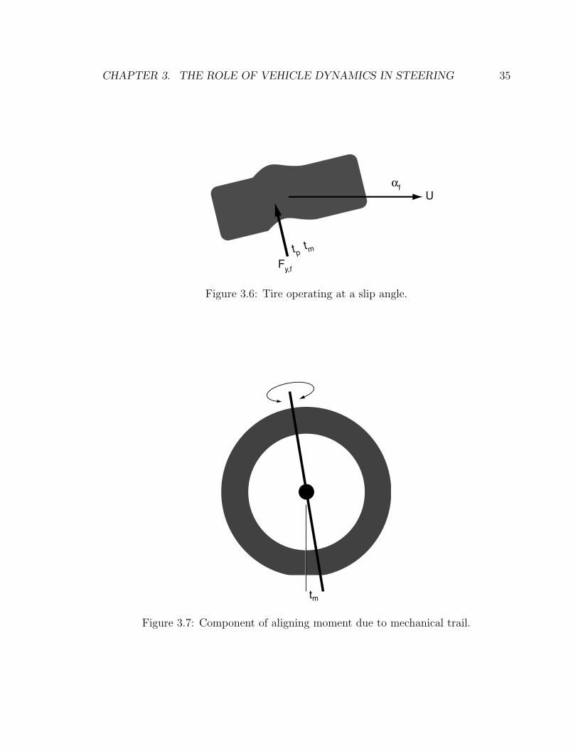
forces. In Figure 3.6, Fy,f is the lateral force acting on the tire, αf is the tire slip
angle, tp is the pneumatic trail, the distance between the application of lateral force
and the center of the tire, tm is the mechanical trail, the distance between the tire
center and the point on the ground about which the tire pivots as a result of the
wheel caster angle (Figure 3.7), and U is the velocity of the tire at its center. The
total aligning moment is given by:
τa = (tp + tm)Fy,f (αf ) (3.9)
CHAPTER 3. THE ROLE OF VEHICLE DYNAMICS IN STEERING 34
10 15 20 25 30 35 40 45 50 55−20
−10
0
10
20
time (s)
stee
ring
angl
e (d
eg) actual
commanded
10 15 20 25 30 35 40 45 50 55−1
−0.5
0
0.5
1
time (s)
stee
ring
angl
e er
ror
(deg
)
Figure 3.5: Error due to aligning moment.
The portion of aligning moment due to the tire pneumatic trail may be directly
approximated as an empirical function of tire slip angle (see Appendix A). Although
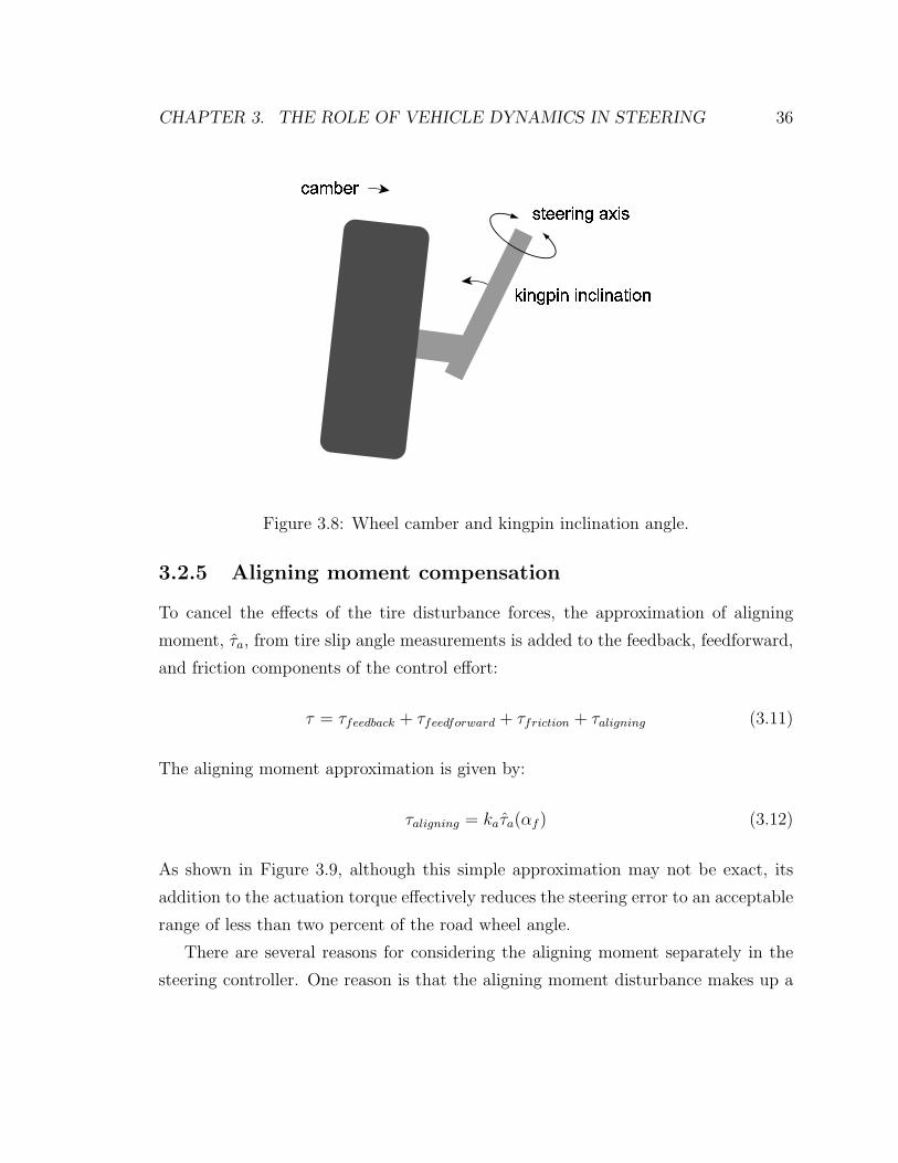
pneumatic trail is also a function of slip angle, it is linear for small angles. The
steering geometry, particularly the kingpin inclination angle and camber angle, will
cause the mechanical trail to vary with steering position (Figure 3.8). Here we assume
a constant mechanical trail. Furthermore, the steering geometry often causes a slight
vertical motion of the wheels—effectively raising and lowering the front of the vehicle
as it is being steered—so that the steering effort must overcome the force of gravity
on the vehicle sprung mass [49]. If the geometry is known, however, most of these
effects can be modelled and accounted for by the controller. When the aligning
moment disturbance, τa, is included, the steering system model given by Equation
(2.7) becomes:
Jsθ + bsθ + Fssgn(θ) = τ − kaτa (3.10)
where ka is a scale factor to account for torque reduction by the steering gear.
CHAPTER 3. THE ROLE OF VEHICLE DYNAMICS IN STEERING 35
tptm
αf
Fy,f
U
Figure 3.6: Tire operating at a slip angle.
tm
Figure 3.7: Component of aligning moment due to mechanical trail.
CHAPTER 3. THE ROLE OF VEHICLE DYNAMICS IN STEERING 36
)*++,-./01-)2034+,
5-./6-.-.27-.0*-8.
Figure 3.8: Wheel camber and kingpin inclination angle.
3.2.5 Aligning moment compensation
To cancel the effects of the tire disturbance forces, the approximation of aligning
moment, τa, from tire slip angle measurements is added to the feedback, feedforward,
and friction components of the control effort:
τ = τfeedback + τfeedforward + τfriction + τaligning (3.11)
The aligning moment approximation is given by:
τaligning = kaτa(αf ) (3.12)
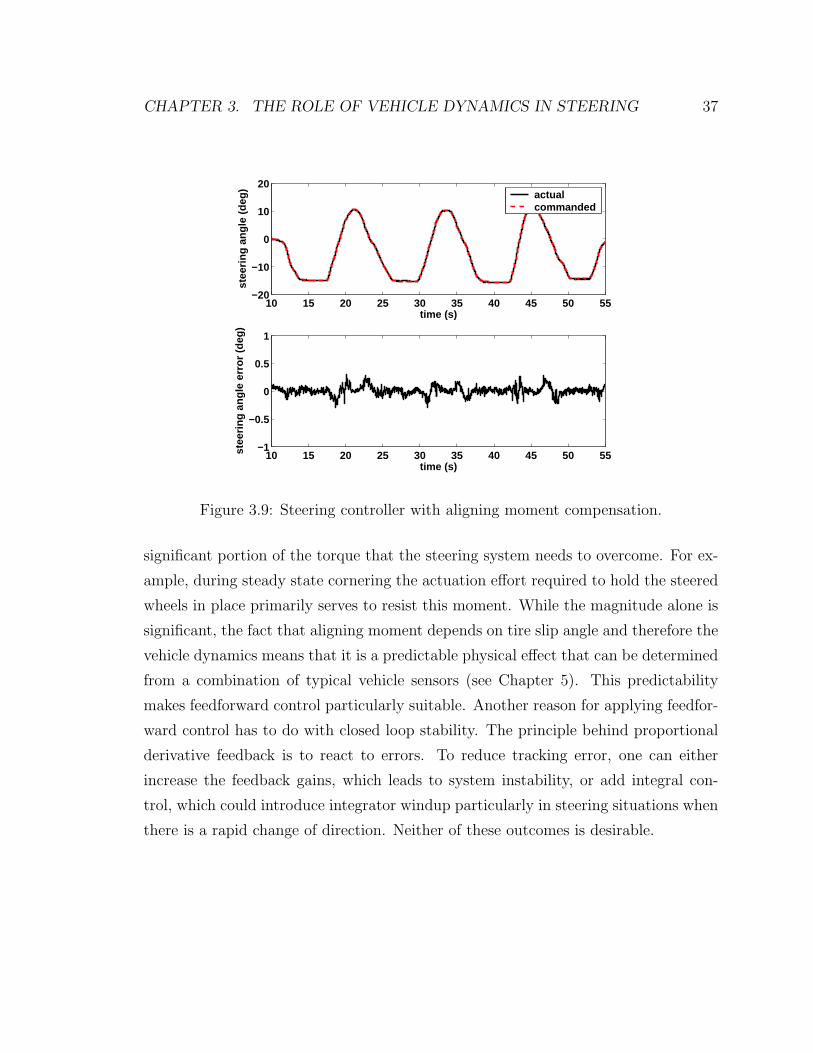
As shown in Figure 3.9, although this simple approximation may not be exact, its
addition to the actuation torque effectively reduces the steering error to an acceptable
range of less than two percent of the road wheel angle.
There are several reasons for considering the aligning moment separately in the
steering controller. One reason is that the aligning moment disturbance makes up a
CHAPTER 3. THE ROLE OF VEHICLE DYNAMICS IN STEERING 37
10 15 20 25 30 35 40 45 50 55−20
−10
0
10
20
time (s)
stee
ring
angl
e (d
eg) actual
commanded
10 15 20 25 30 35 40 45 50 55−1
−0.5
0
0.5
1
time (s)
stee
ring
angl
e er
ror
(deg
)
Figure 3.9: Steering controller with aligning moment compensation.
significant portion of the torque that the steering system needs to overcome. For ex-
ample, during steady state cornering the actuation effort required to hold the steered
wheels in place primarily serves to resist this moment. While the magnitude alone is
significant, the fact that aligning moment depends on tire slip angle and therefore the
vehicle dynamics means that it is a predictable physical effect that can be determined
from a combination of typical vehicle sensors (see Chapter 5). This predictability
makes feedforward control particularly suitable. Another reason for applying feedfor-
ward control has to do with closed loop stability. The principle behind proportional
derivative feedback is to react to errors. To reduce tracking error, one can either
increase the feedback gains, which leads to system instability, or add integral con-
trol, which could introduce integrator windup particularly in steering situations when
there is a rapid change of direction. Neither of these outcomes is desirable.
CHAPTER 3. THE ROLE OF VEHICLE DYNAMICS IN STEERING 38
Js
bs
Fs
Kd
Kp
steering
system vehicle
dynamics
sgn
θ++
+ + τ
+- +
+
+
θ
θd
αf
τaligning
ka
τfriction
τfeedforward
τa
τfeedback
1st order
filter
2nd order
filter
1st order
filter
1st order
filter
1st order
filter
θd
θd
θd
θd
+-
Figure 3.10: Steering controller block diagram.
3.3 Combined control
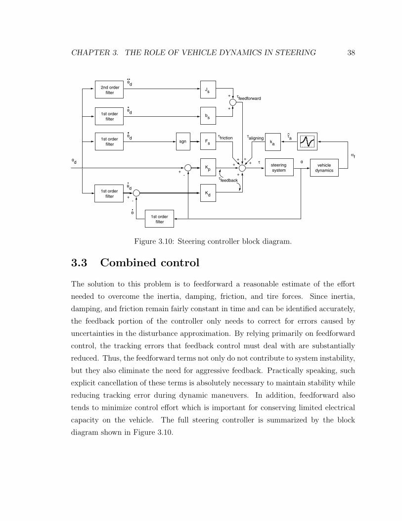
The solution to this problem is to feedforward a reasonable estimate of the effort
needed to overcome the inertia, damping, friction, and tire forces. Since inertia,
damping, and friction remain fairly constant in time and can be identified accurately,
the feedback portion of the controller only needs to correct for errors caused by
uncertainties in the disturbance approximation. By relying primarily on feedforward
control, the tracking errors that feedback control must deal with are substantially
reduced. Thus, the feedforward terms not only do not contribute to system instability,
but they also eliminate the need for aggressive feedback. Practically speaking, such
explicit cancellation of these terms is absolutely necessary to maintain stability while
reducing tracking error during dynamic maneuvers. In addition, feedforward also
tends to minimize control effort which is important for conserving limited electrical
capacity on the vehicle. The full steering controller is summarized by the block
diagram shown in Figure 3.10.
CHAPTER 3. THE ROLE OF VEHICLE DYNAMICS IN STEERING 39
3.3.1 Error dynamics
The effectiveness of this control form can be easily seen in the error dynamics, which
are determined by combining Equations (3.10) and (3.11),
e =1
Js
(Kpe + Kde) + [Fssgn(θd) − Fssgn(θ) + kaτa − kaτa]
=1
Js
(Kpe + Kde) + δe (3.13)
where the error, e, is given by:
e = θd − θ (3.14)
Aside from some uncertainties, δe, in compensating for the friction and tire aligning
moment, the error dynamics are stable and approach zero quickly if Kp and Kd
are chosen appropriately. Even with approximate values of the Coulomb friction
constant, Fs, and aligning moment, τa, the controller can produce good tracking
results, which suggests that it is robust to disturbances and variations in the steering
system parameters.
Chapter 4
A means to influence vehicle
handling
A vehicle’s handling characteristics are dictated by its physical parameters: wheel-
base, track width, center of gravity location, mass, moment of inertia, suspension
design, and tire properties. Without active control, the only way to change how a ve-
hicle handles is to alter one or more of these physical parameters. Such changes may
involve significant design considerations and typically cannot be done “on the fly.”
The theme of this chapter offers exactly this possibility: with a combination of active
steering capability and feedback control, a vehicle’s response to the driver’s inputs
can be modified though the physical parameters of the vehicle remain unchanged.
In other words, the application of dynamic feedback can modify the vehicle states so
that, from the driver’s perspective, the vehicle has a fundamentally different handling
characteristic. This idea is compelling from a design viewpoint, since a near infinite
number of physical design variations can be evaluated on a single platform [42, 27].
More practically, a vehicle with such a system could automatically compensate for
unforseen changes in physical parameters (i.e. mass and weight distribution due to
loading) as well as changes in operating conditions (i.e. road friction) that might
otherwise have a deleterious effect on handling behavior [20]. This chapter presents
one way in which feedback of vehicle sideslip angle and yaw rate combined with active
steering capability may be used to modify a vehicle’s handling characteristics.
40
CHAPTER 4. A MEANS TO INFLUENCE VEHICLE HANDLING 41
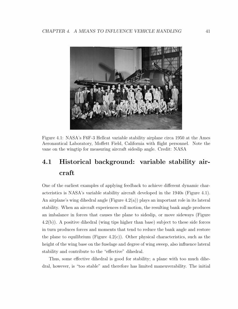
Figure 4.1: NASA’s F6F-3 Hellcat variable stability airplane circa 1950 at the AmesAeronautical Laboratory, Moffett Field, California with flight personnel. Note thevane on the wingtip for measuring aircraft sideslip angle. Credit: NASA
4.1 Historical background: variable stability air-
craft
One of the earliest examples of applying feedback to achieve different dynamic char-
acteristics is NASA’s variable stability aircraft developed in the 1940s (Figure 4.1).
An airplane’s wing dihedral angle (Figure 4.2(a)) plays an important role in its lateral
stability. When an aircraft experiences roll motion, the resulting bank angle produces
an imbalance in forces that causes the plane to sideslip, or move sideways (Figure
4.2(b)). A positive dihedral (wing tips higher than base) subject to these side forces
in turn produces forces and moments that tend to reduce the bank angle and restore
the plane to equilibrium (Figure 4.2(c)). Other physical characteristics, such as the
height of the wing base on the fuselage and degree of wing sweep, also influence lateral
stability and contribute to the “effective” dihedral.
Thus, some effective dihedral is good for stability; a plane with too much dihe-
dral, however, is “too stable” and therefore has limited maneuverability. The initial
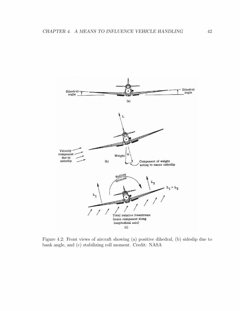
CHAPTER 4. A MEANS TO INFLUENCE VEHICLE HANDLING 42
Figure 4.2: Front views of aircraft showing (a) positive dihedral, (b) sideslip due tobank angle, and (c) stabilizing roll moment. Credit: NASA
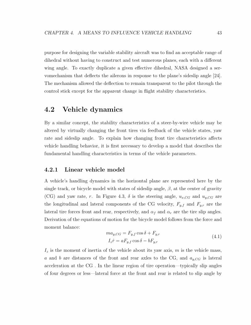
CHAPTER 4. A MEANS TO INFLUENCE VEHICLE HANDLING 43
purpose for designing the variable stability aircraft was to find an acceptable range of
dihedral without having to construct and test numerous planes, each with a different
wing angle. To exactly duplicate a given effective dihedral, NASA designed a ser-
vomechanism that deflects the ailerons in response to the plane’s sideslip angle [24].
The mechanism allowed the deflection to remain transparent to the pilot through the
control stick except for the apparent change in flight stability characteristics.
4.2 Vehicle dynamics
By a similar concept, the stability characteristics of a steer-by-wire vehicle may be
altered by virtually changing the front tires via feedback of the vehicle states, yaw
rate and sideslip angle. To explain how changing front tire characteristics affects
vehicle handling behavior, it is first necessary to develop a model that describes the
fundamental handling characteristics in terms of the vehicle parameters.
4.2.1 Linear vehicle model
A vehicle’s handling dynamics in the horizontal plane are represented here by the
single track, or bicycle model with states of sideslip angle, β, at the center of gravity
(CG) and yaw rate, r. In Figure 4.3, δ is the steering angle, ux,CG and uy,CG are
the longitudinal and lateral components of the CG velocity, Fy,f and Fy,r are the
lateral tire forces front and rear, respectively, and αf and αr are the tire slip angles.
Derivation of the equations of motion for the bicycle model follows from the force and
moment balance:may,CG = Fy,f cos δ + Fy,r
Iz r = aFy,f cos δ − bFy,r
(4.1)
Iz is the moment of inertia of the vehicle about its yaw axis, m is the vehicle mass,
a and b are distances of the front and rear axles to the CG, and ay,CG is lateral
acceleration at the CG . In the linear region of tire operation—typically slip angles
of four degrees or less—lateral force at the front and rear is related to slip angle by
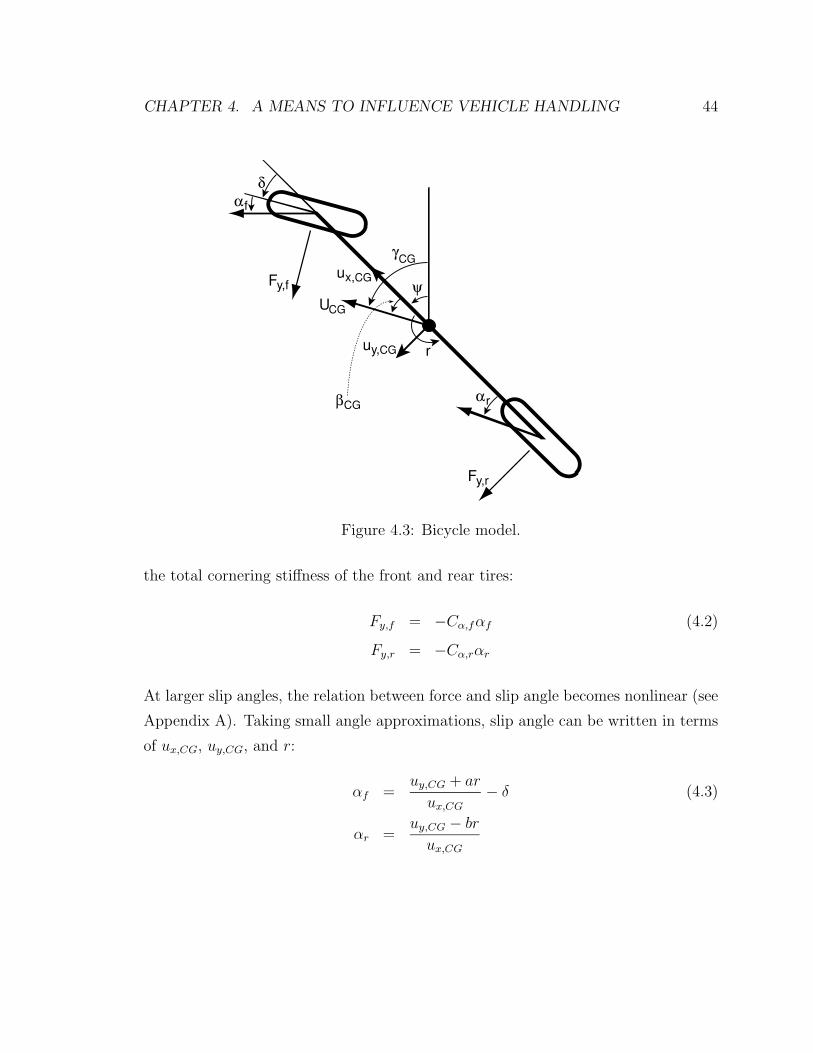
CHAPTER 4. A MEANS TO INFLUENCE VEHICLE HANDLING 44
δ
αf
r
αr
uy,CG
ux,CG
Fy,r
Fy,f
βCG
γCG
ψUCG
Figure 4.3: Bicycle model.
the total cornering stiffness of the front and rear tires:
Fy,f = −Cα,fαf (4.2)
Fy,r = −Cα,rαr
At larger slip angles, the relation between force and slip angle becomes nonlinear (see
Appendix A). Taking small angle approximations, slip angle can be written in terms
of ux,CG, uy,CG, and r:
αf =uy,CG + ar
ux,CG
− δ (4.3)
αr =uy,CG − br
ux,CG
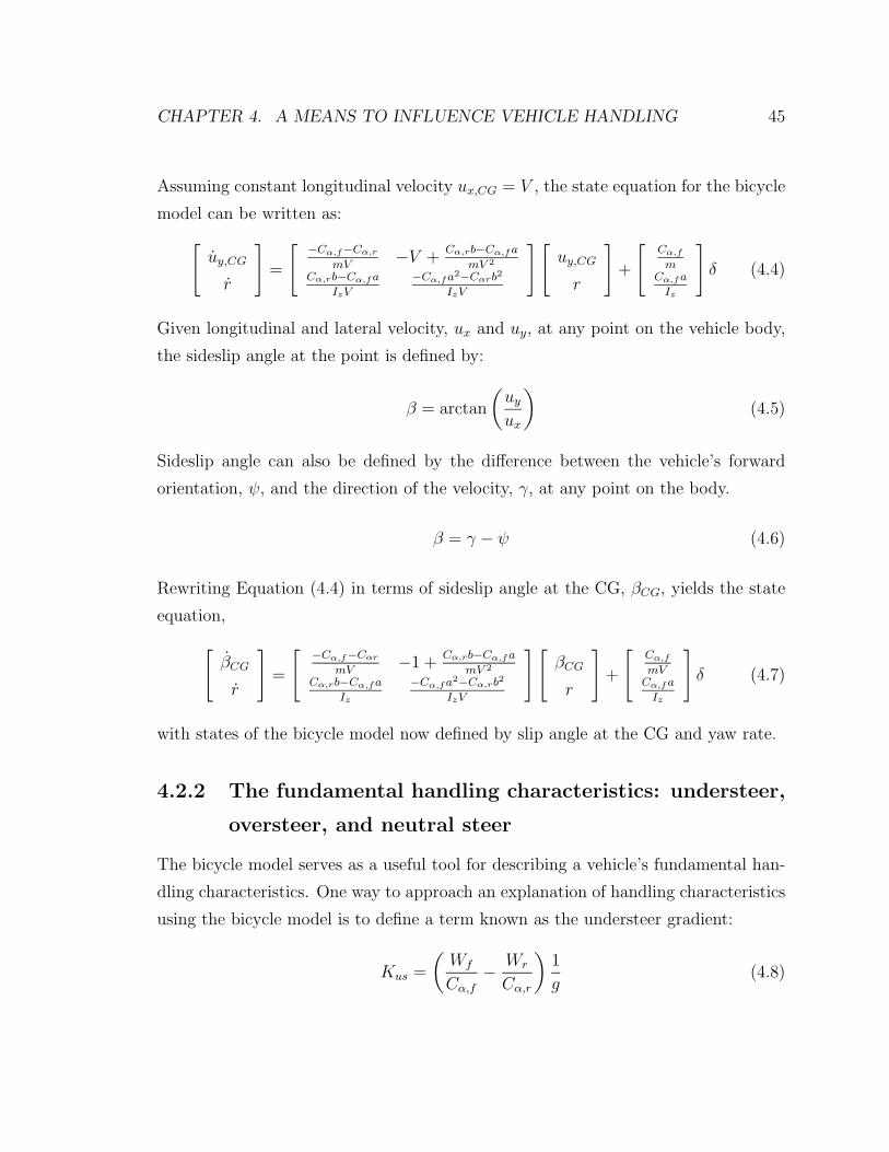
CHAPTER 4. A MEANS TO INFLUENCE VEHICLE HANDLING 45
Assuming constant longitudinal velocity ux,CG = V , the state equation for the bicycle
model can be written as:
[
uy,CG
r
]
=
[
−Cα,f−Cα,r
mV−V +
Cα,rb−Cα,fa
mV 2
Cα,rb−Cα,f a
IzV
−Cα,f a2−Cαrb2
IzV
][
uy,CG
r
]
+
[
Cα,f
mCα,f a
Iz
]
δ (4.4)
Given longitudinal and lateral velocity, ux and uy, at any point on the vehicle body,
the sideslip angle at the point is defined by:
β = arctan
(
uy
ux
)
(4.5)
Sideslip angle can also be defined by the difference between the vehicle’s forward
orientation, ψ, and the direction of the velocity, γ, at any point on the body.
β = γ − ψ (4.6)
Rewriting Equation (4.4) in terms of sideslip angle at the CG, βCG, yields the state
equation,
[
βCG
r
]
=
[
−Cα,f−Cαr
mV−1 +
Cα,rb−Cα,f a
mV 2
Cα,rb−Cα,f a
Iz
−Cα,f a2−Cα,rb2
IzV
][
βCG
r
]
+
[
Cα,f
mVCα,f a
Iz
]
δ (4.7)
with states of the bicycle model now defined by slip angle at the CG and yaw rate.
4.2.2 The fundamental handling characteristics: understeer,
oversteer, and neutral steer
The bicycle model serves as a useful tool for describing a vehicle’s fundamental han-
dling characteristics. One way to approach an explanation of handling characteristics
using the bicycle model is to define a term known as the understeer gradient:
Kus =
(
Wf
Cα,f
−Wr
Cα,r
)
1
g(4.8)
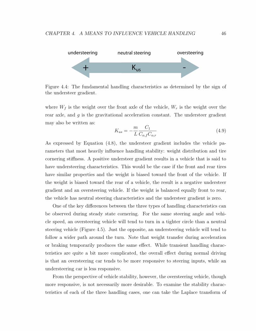
CHAPTER 4. A MEANS TO INFLUENCE VEHICLE HANDLING 46
Kus -+
understeering neutral steering oversteering
Figure 4.4: The fundamental handling characteristics as determined by the sign ofthe understeer gradient.
where Wf is the weight over the front axle of the vehicle, Wr is the weight over the
rear axle, and g is the gravitational acceleration constant. The understeer gradient
may also be written as:
Kus = −m
L
C1
Cα,fCα,r
(4.9)
As expressed by Equation (4.8), the understeer gradient includes the vehicle pa-
rameters that most heavily influence handling stability: weight distribution and tire
cornering stiffness. A positive understeer gradient results in a vehicle that is said to
have understeering characteristics. This would be the case if the front and rear tires
have similar properties and the weight is biased toward the front of the vehicle. If
the weight is biased toward the rear of a vehicle, the result is a negative understeer
gradient and an oversteering vehicle. If the weight is balanced equally front to rear,
the vehicle has neutral steering characteristics and the understeer gradient is zero.
One of the key differences between the three types of handling characteristics can
be observed during steady state cornering. For the same steering angle and vehi-
cle speed, an oversteering vehicle will tend to turn in a tighter circle than a neutral
steering vehicle (Figure 4.5). Just the opposite, an understeering vehicle will tend to
follow a wider path around the turn. Note that weight transfer during acceleration
or braking temporarily produces the same effect. While transient handling charac-
teristics are quite a bit more complicated, the overall effect during normal driving
is that an oversteering car tends to be more responsive to steering inputs, while an
understeering car is less responsive.
From the perspective of vehicle stability, however, the oversteering vehicle, though
more responsive, is not necessarily more desirable. To examine the stability charac-
teristics of each of the three handling cases, one can take the Laplace transform of
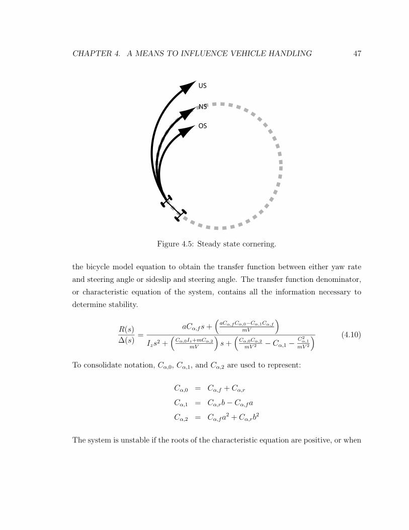
CHAPTER 4. A MEANS TO INFLUENCE VEHICLE HANDLING 47
OS
NS
US
Figure 4.5: Steady state cornering.
the bicycle model equation to obtain the transfer function between either yaw rate
and steering angle or sideslip and steering angle. The transfer function denominator,
or characteristic equation of the system, contains all the information necessary to
determine stability.
R(s)
∆(s)=
aCα,fs +(
aCα,f Cα,0−Cα,1Cα,f
mV
)
Izs2 +(
Cα,0Iz+mCα,2
mV
)
s +(
Cα,0Cα,2
mV 2 − Cα,1 −C2
α,1
mV 2
) (4.10)
To consolidate notation, Cα,0, Cα,1, and Cα,2 are used to represent:
Cα,0 = Cα,f + Cα,r
Cα,1 = Cα,rb − Cα,fa
Cα,2 = Cα,fa2 + Cα,rb
2
The system is unstable if the roots of the characteristic equation are positive, or when
CHAPTER 4. A MEANS TO INFLUENCE VEHICLE HANDLING 48
the third term in the denominator is less than zero:
Cα,0Cα,2
mV 2− Cα,1 −
C2α,1
mV 2< 0 (4.11)
Since vehicle speed, V , is always positive, this also means that:
Cα,0Cα,2 − C2
α,1 − Cα,1mV 2 < 0 (4.12)
Substituting for Cα,0, Cα,1, and Cα,2 yields:
L2Cα,fCα,r − Cα,1mV 2 < 0 (4.13)
where L = a+b is the wheelbase length. This can be simplified further by rearranging
Equation (4.9) and substituting for the remaining Cα,1 term:
L2 + KusV2 < 0 (4.14)
The inequality is only valid if the understeer gradient, Kus, is negative (the vehicle is
oversteering) and the speed is above the critical speed, defined by:
Vcr =
√
−L
Kus
(4.15)
Therefore, the unstable condition does not exist for a vehicle with understeering or
neutral steering characteristics. According to the linear vehicle model, instability
occurs when an oversteering vehicle is travelling faster than its critical speed.
Passenger vehicles are never designed to have oversteering characteristics for this
reason. In fact, most vehicles are designed with characteristics solidly in the under-
steering range of the handling scale: this is to provide a margin of safety in case, for
example, passengers or cargo move the weight distribution rearward and therefore
shift the handling behavior toward the oversteering end of the scale. Some types of
vehicles, such as 15-passenger vans, are particularly susceptible to this problem [50].
To a lesser extent, differences in tire cornering stiffness between the front and rear due
CHAPTER 4. A MEANS TO INFLUENCE VEHICLE HANDLING 49
to wear or tread characteristics can have a similar effect. Since a vehicle’s handling
characteristics are inherent to its physical design, there will always be a design trade-
off between the stability and predictability of heavily understeering behavior and the
responsiveness and potential instability of marginally understeering, neutral steering,
or oversteering characteristics.
An important distinction should be made between oversteering as a handling
characteristic and the term “limit oversteer,” which describes the situation during
cornering when the rear tires lose their grip on the pavement before the front tires.
This behavior occurs outside of the linear handling region described by the linear tire
force model (Fy = Cα,fαf ). If not corrected quickly enough, a vehicle undergoing limit
oversteer will fishtail or spin out. Similarly, the term “limit understeer” refers to the
opposite condition: the front tires reach the limits of adhesion before the rear tires,
and the vehicle no longer responds to increasing steering angles. Any vehicle, whether
understeering, neutral steering, or oversteering, can potentially experience either of
these situations given the right (or wrong) driving conditions. During normal street
driving, a vehicle almost never ventures into nonlinear handling territory. Limit
oversteer and understeer are mainly of concern during emergency maneuvers, high
performance driving, or on very slippery surfaces such as snow or ice. These situations
involving transition to nonlinear tire characteristics will be addressed later in the
thesis, as they are exactly analogous to the linear case.
4.3 Handling modification
4.3.1 Full state feedback: a virtual tire change
The full state feedback control law for an active steering vehicle is given by:
δ = Krr + Kββ + Kdδd (4.16)
where δd is the driver’s steering angle measured at the handwheel and δ is the actual
steering angle commanded by the controller. A physically intuitive way to modify a
CHAPTER 4. A MEANS TO INFLUENCE VEHICLE HANDLING 50
vehicle’s handling characteristics is to define a target front cornering stiffness as:
Cα,f = Cα,f (1 + η) (4.17)
and the state feedback gains as:
Kβ = −η Kr = −a
Vη Kd = (1 + η) (4.18)
where η is the desired fractional change in the original front cornering stiffness, Cα,f .
Substituting the feedback law, Equation (4.16), into Equation (4.7) yields a state
space equation of the same form as Equation (4.7) but with the new cornering stiffness,
Cα,f :
[
βCG
r
]
=
[
−Cα,f−Cαr
mV−1 +
Cα,rb−Cα,f a
mV 2
Cα,rb−Cα,f a
Iz
−Cα,f a2−Cα,rb2
IzV
][
βCG
r
]
+
[
Cα,f
mVCα,f a
Iz
]
δ (4.19)
Since a vehicle’s handling characteristics are directly influenced by tire cornering stiff-
ness, the effect of this modification is to make the vehicle either more oversteering
or understeering depending on the sign of η. Of course, there are many other ways
to apply full state feedback, but the physical motivation behind cornering stiffness
adjustment makes clear through the bicycle model exactly how the handling charac-
teristics have been modified. In fact, the effect of this modification is analogous to a
common practice in automotive racing: changing tires during a pit stop to adjust a
race car’s handling dynamics.
A question that naturally arises from this form of vehicle dynamics control is
whether similar handling changes can be achieved given only yaw rate feedback.
Although yaw rate feedback is frequently proposed [23] [3] [48] as a way to control
gross vehicle motion, yaw rate feedback alone leaves sideslip uncontrolled. It then
becomes possible to change the vehicle transfer function to something that is neither
physically realizable nor intuitive to the driver, and the effects of this are unclear.
Furthermore, in extreme cases there may be good yaw tracking but excessive sideslip
[1]. As mentioned before, this type of situation falls outside the realm of safe handling
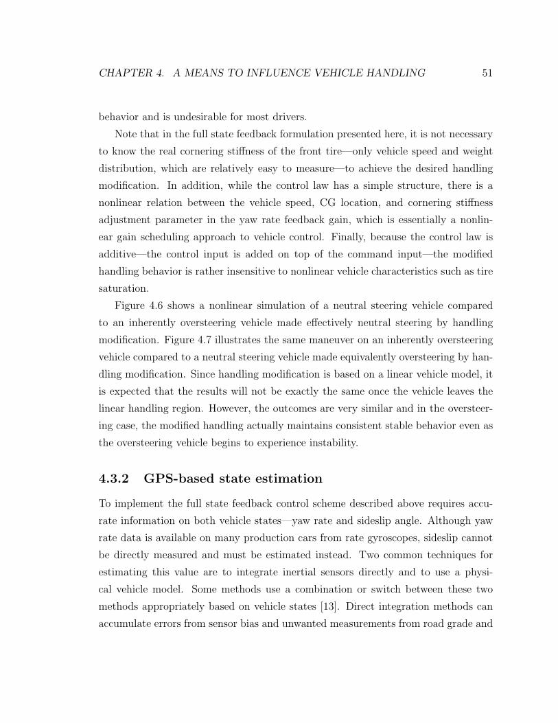
CHAPTER 4. A MEANS TO INFLUENCE VEHICLE HANDLING 51
behavior and is undesirable for most drivers.
Note that in the full state feedback formulation presented here, it is not necessary
to know the real cornering stiffness of the front tire—only vehicle speed and weight
distribution, which are relatively easy to measure—to achieve the desired handling
modification. In addition, while the control law has a simple structure, there is a
nonlinear relation between the vehicle speed, CG location, and cornering stiffness
adjustment parameter in the yaw rate feedback gain, which is essentially a nonlin-
ear gain scheduling approach to vehicle control. Finally, because the control law is
additive—the control input is added on top of the command input—the modified
handling behavior is rather insensitive to nonlinear vehicle characteristics such as tire
saturation.
Figure 4.6 shows a nonlinear simulation of a neutral steering vehicle compared
to an inherently oversteering vehicle made effectively neutral steering by handling
modification. Figure 4.7 illustrates the same maneuver on an inherently oversteering
vehicle compared to a neutral steering vehicle made equivalently oversteering by han-
dling modification. Since handling modification is based on a linear vehicle model, it
is expected that the results will not be exactly the same once the vehicle leaves the
linear handling region. However, the outcomes are very similar and in the oversteer-
ing case, the modified handling actually maintains consistent stable behavior even as
the oversteering vehicle begins to experience instability.
4.3.2 GPS-based state estimation
To implement the full state feedback control scheme described above requires accu-
rate information on both vehicle states—yaw rate and sideslip angle. Although yaw
rate data is available on many production cars from rate gyroscopes, sideslip cannot
be directly measured and must be estimated instead. Two common techniques for
estimating this value are to integrate inertial sensors directly and to use a physi-
cal vehicle model. Some methods use a combination or switch between these two
methods appropriately based on vehicle states [13]. Direct integration methods can
accumulate errors from sensor bias and unwanted measurements from road grade and

CHAPTER 4. A MEANS TO INFLUENCE VEHICLE HANDLING 52
0 5 10 15 20−40
−20
0
20
40
time (s)
yaw
rat
e (d
eg/s
)
normalmodified
0 5 10 15 20−2
−1
0
1
2
time (s)
side
slip
ang
le (
deg)
Figure 4.6: Nonlinear vehicle simulation with and without handling modification:neutral steering case.
0 5 10 15 20−40
−20
0
20
40
time (s)
yaw
rat
e (d
eg/s
)
normalmodified
0 5 10 15 20−2
−1
0
1
2
time (s)
side
slip
ang
le (
deg)
Figure 4.7: Nonlinear vehicle simulation with and without handling modification:oversteering case.
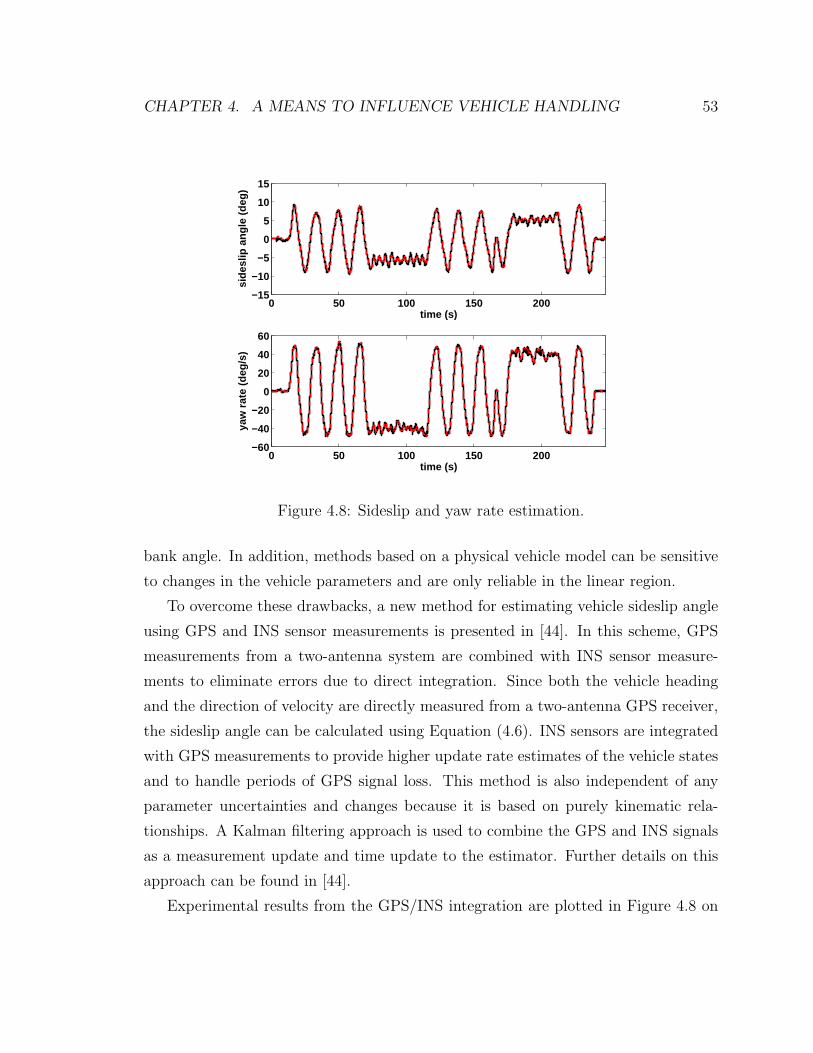
CHAPTER 4. A MEANS TO INFLUENCE VEHICLE HANDLING 53
0 50 100 150 200−15
−10
−5
0
5
10
15
time (s)
side
slip
ang
le (
deg)
0 50 100 150 200−60
−40
−20
0
20
40
60
time (s)
yaw
rat
e (d
eg/s
)
Figure 4.8: Sideslip and yaw rate estimation.
bank angle. In addition, methods based on a physical vehicle model can be sensitive
to changes in the vehicle parameters and are only reliable in the linear region.
To overcome these drawbacks, a new method for estimating vehicle sideslip angle
using GPS and INS sensor measurements is presented in [44]. In this scheme, GPS
measurements from a two-antenna system are combined with INS sensor measure-
ments to eliminate errors due to direct integration. Since both the vehicle heading
and the direction of velocity are directly measured from a two-antenna GPS receiver,
the sideslip angle can be calculated using Equation (4.6). INS sensors are integrated
with GPS measurements to provide higher update rate estimates of the vehicle states
and to handle periods of GPS signal loss. This method is also independent of any
parameter uncertainties and changes because it is based on purely kinematic rela-
tionships. A Kalman filtering approach is used to combine the GPS and INS signals
as a measurement update and time update to the estimator. Further details on this
approach can be found in [44].
Experimental results from the GPS/INS integration are plotted in Figure 4.8 on
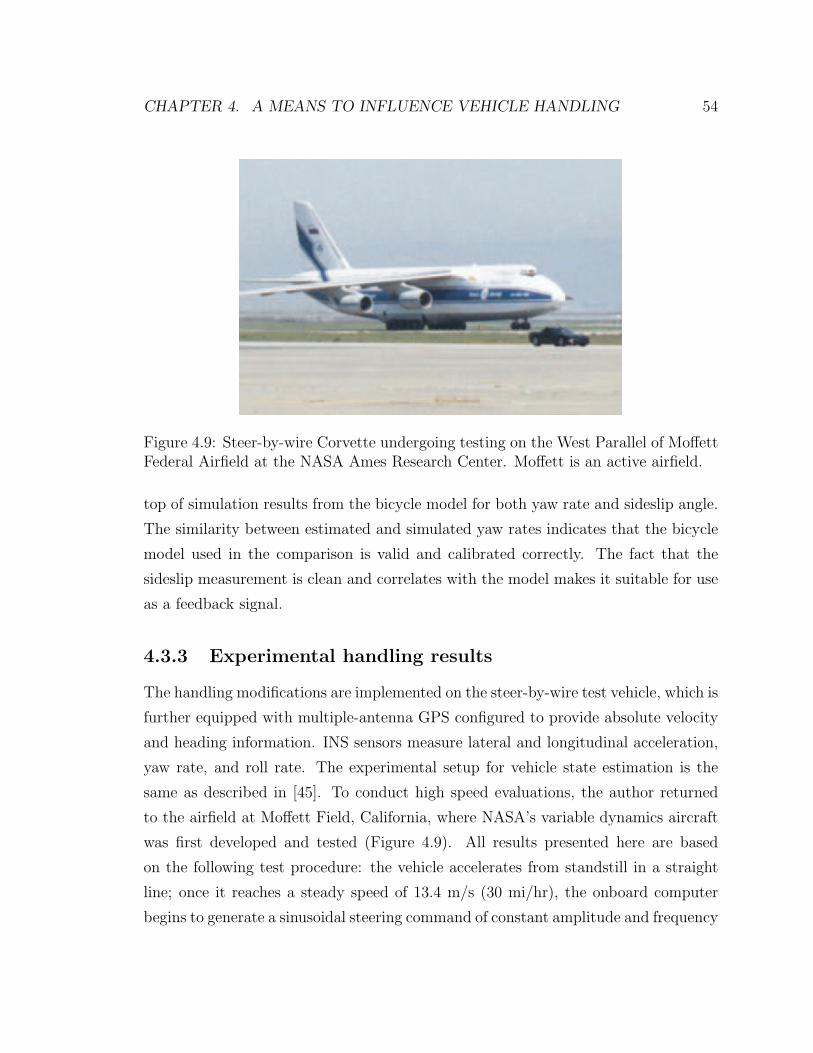
CHAPTER 4. A MEANS TO INFLUENCE VEHICLE HANDLING 54
Figure 4.9: Steer-by-wire Corvette undergoing testing on the West Parallel of MoffettFederal Airfield at the NASA Ames Research Center. Moffett is an active airfield.
top of simulation results from the bicycle model for both yaw rate and sideslip angle.
The similarity between estimated and simulated yaw rates indicates that the bicycle
model used in the comparison is valid and calibrated correctly. The fact that the
sideslip measurement is clean and correlates with the model makes it suitable for use
as a feedback signal.
4.3.3 Experimental handling results
The handling modifications are implemented on the steer-by-wire test vehicle, which is
further equipped with multiple-antenna GPS configured to provide absolute velocity
and heading information. INS sensors measure lateral and longitudinal acceleration,
yaw rate, and roll rate. The experimental setup for vehicle state estimation is the
same as described in [45]. To conduct high speed evaluations, the author returned
to the airfield at Moffett Field, California, where NASA’s variable dynamics aircraft
was first developed and tested (Figure 4.9). All results presented here are based
on the following test procedure: the vehicle accelerates from standstill in a straight
line; once it reaches a steady speed of 13.4 m/s (30 mi/hr), the onboard computer
begins to generate a sinusoidal steering command of constant amplitude and frequency
CHAPTER 4. A MEANS TO INFLUENCE VEHICLE HANDLING 55
5 10 15 20 25−40
−30
−20
−10
0
10
20
30
40
time (s)
yaw
rat
e (d
eg/s
)
simulationexperiment
Figure 4.10: Comparison between yaw rate of bicycle model and experiment withnormal cornering stiffness.
(equivalent to a driver’s input at the steering wheel). For the first test, the vehicle
is driven in the unmodified mode (no state feedback) such that the road wheel angle
corresponds directly to command angle scaled by the steering ratio. In Figure 4.10,
the measured yaw rate for this test compares well to simulation results from the
bicycle model. Figure 4.11 shows the sideslip comparison for the same test data.
Convergence of the state estimator causes some deviation from the simulation in the
first few cycles. The sideslip data is also somewhat noisy due to unevenness in the
pavement used for testing. However, given that the sideslip angle being measured is
around one degree or less, the results match extremely well.
Changes in handling behavior under full state feedback control are evaluated by
comparing measured vehicle response to the nominal case shown in Figures 4.10 and
4.11. In Figure 4.12, the effective front cornering stiffness is reduced 50% by setting
the parameter η to -0.5, and the steering input has been modified by the control law to
achieve exactly this characteristic. The experimental results exhibit lower peak yaw
rate and lateral acceleration values than the nominal case (Figures 4.13 and 4.14).
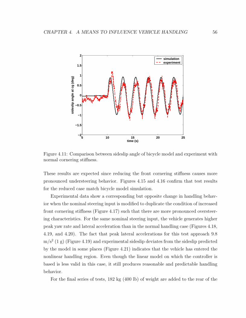
CHAPTER 4. A MEANS TO INFLUENCE VEHICLE HANDLING 56
5 10 15 20 25−2
−1.5
−1
−0.5
0
0.5
1
1.5
2
time (s)
side
slip
ang
le a
t cg
(deg
)
simulationexperiment
Figure 4.11: Comparison between sideslip angle of bicycle model and experiment withnormal cornering stiffness.
These results are expected since reducing the front cornering stiffness causes more
pronounced understeering behavior. Figures 4.15 and 4.16 confirm that test results
for the reduced case match bicycle model simulation.
Experimental data show a corresponding but opposite change in handling behav-
ior when the nominal steering input is modified to duplicate the condition of increased
front cornering stiffness (Figure 4.17) such that there are more pronounced oversteer-
ing characteristics. For the same nominal steering input, the vehicle generates higher
peak yaw rate and lateral acceleration than in the normal handling case (Figures 4.18,
4.19, and 4.20). The fact that peak lateral accelerations for this test approach 9.8
m/s2 (1 g) (Figure 4.19) and experimental sideslip deviates from the sideslip predicted
by the model in some places (Figure 4.21) indicates that the vehicle has entered the
nonlinear handling region. Even though the linear model on which the controller is
based is less valid in this case, it still produces reasonable and predictable handling
behavior.
For the final series of tests, 182 kg (400 lb) of weight are added to the rear of the
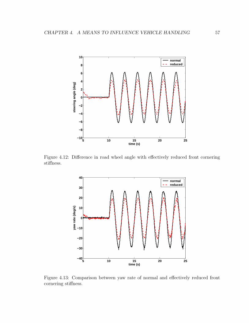
CHAPTER 4. A MEANS TO INFLUENCE VEHICLE HANDLING 57
5 10 15 20 25−10
−8
−6
−4
−2
0
2
4
6
8
10
time (s)
stee
ring
angl
e (d
eg)
normalreduced
Figure 4.12: Difference in road wheel angle with effectively reduced front corneringstiffness.
5 10 15 20 25−40
−30
−20
−10
0
10
20
30
40
time (s)
yaw
rat
e (d
eg/s
)
normalreduced
Figure 4.13: Comparison between yaw rate of normal and effectively reduced frontcornering stiffness.
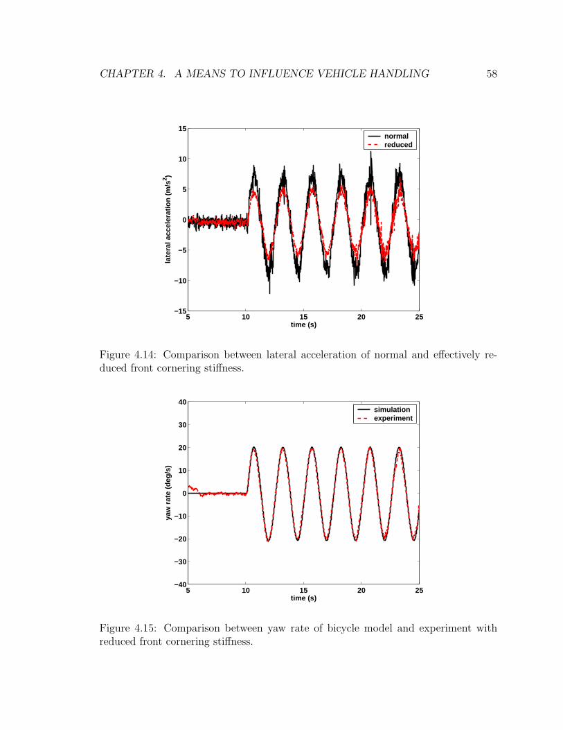
CHAPTER 4. A MEANS TO INFLUENCE VEHICLE HANDLING 58
5 10 15 20 25−15
−10
−5
0
5
10
15
time (s)
late
ral a
ccel
erat
ion
(m/s
2 )
normalreduced
Figure 4.14: Comparison between lateral acceleration of normal and effectively re-duced front cornering stiffness.
5 10 15 20 25−40
−30
−20
−10
0
10
20
30
40
time (s)
yaw
rat
e (d
eg/s
)
simulationexperiment
Figure 4.15: Comparison between yaw rate of bicycle model and experiment withreduced front cornering stiffness.
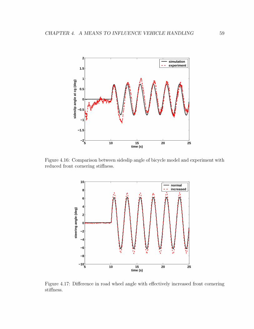
CHAPTER 4. A MEANS TO INFLUENCE VEHICLE HANDLING 59
5 10 15 20 25−2
−1.5
−1
−0.5
0
0.5
1
1.5
2
time (s)
side
slip
ang
le a
t cg
(deg
)
simulationexperiment
Figure 4.16: Comparison between sideslip angle of bicycle model and experiment withreduced front cornering stiffness.
5 10 15 20 25−10
−8
−6
−4
−2
0
2
4
6
8
10
time (s)
stee
ring
angl
e (d
eg)
normalincreased
Figure 4.17: Difference in road wheel angle with effectively increased front corneringstiffness.
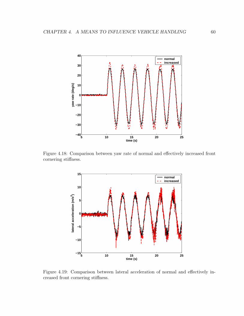
CHAPTER 4. A MEANS TO INFLUENCE VEHICLE HANDLING 60
5 10 15 20 25−40
−30
−20
−10
0
10
20
30
40
time (s)
yaw
rat
e (d
eg/s
)
normalincreased
Figure 4.18: Comparison between yaw rate of normal and effectively increased frontcornering stiffness.
5 10 15 20 25−15
−10
−5
0
5
10
15
time (s)
late
ral a
ccel
erat
ion
(m/s
2 )
normalincreased
Figure 4.19: Comparison between lateral acceleration of normal and effectively in-creased front cornering stiffness.
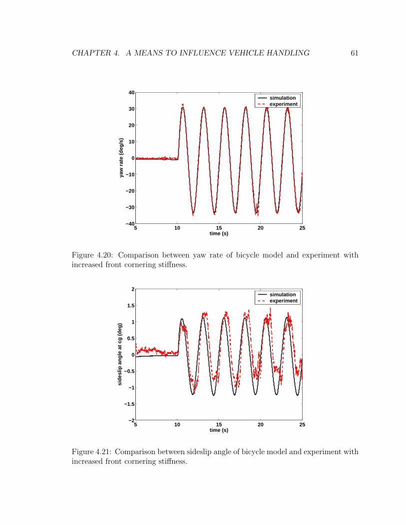
CHAPTER 4. A MEANS TO INFLUENCE VEHICLE HANDLING 61
5 10 15 20 25−40
−30
−20
−10
0
10
20
30
40
time (s)
yaw
rat
e (d
eg/s
)
simulationexperiment
Figure 4.20: Comparison between yaw rate of bicycle model and experiment withincreased front cornering stiffness.
5 10 15 20 25−2
−1.5
−1
−0.5
0
0.5
1
1.5
2
time (s)
side
slip
ang
le a
t cg
(deg
)
simulationexperiment
Figure 4.21: Comparison between sideslip angle of bicycle model and experiment withincreased front cornering stiffness.
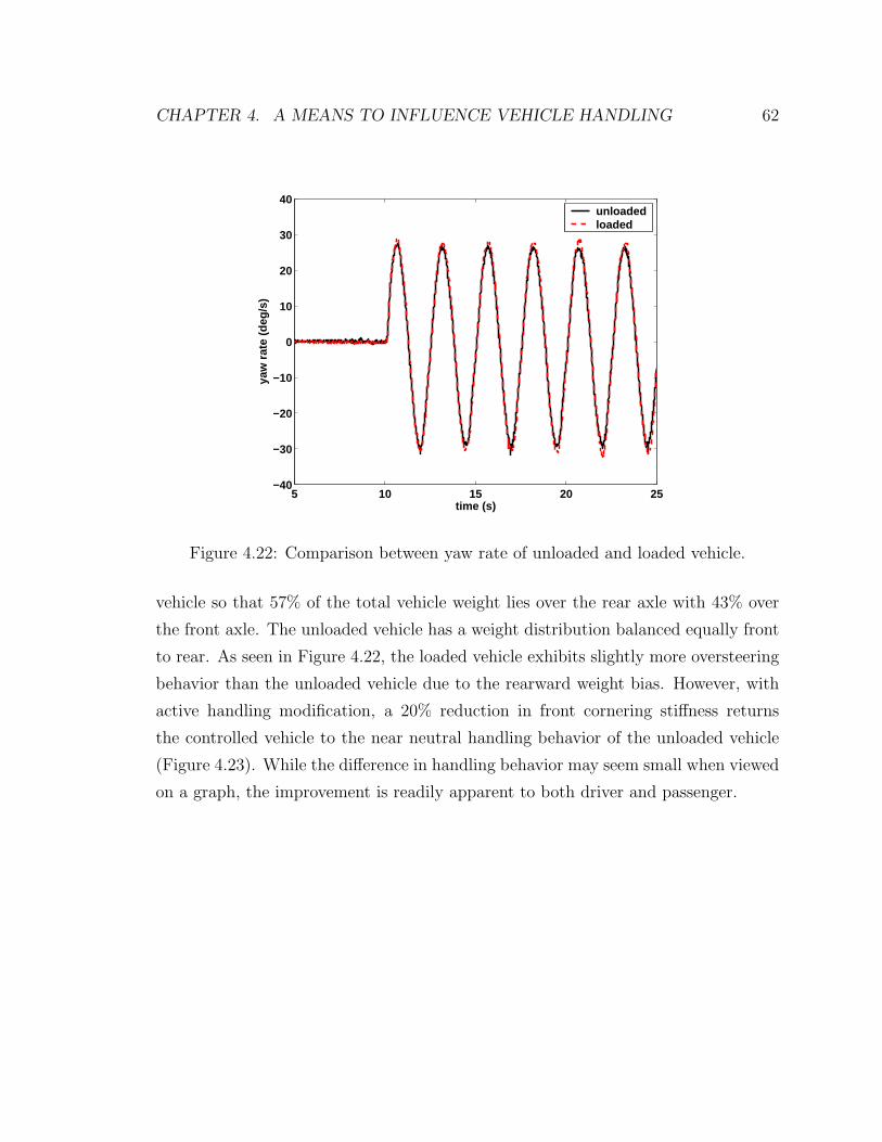
CHAPTER 4. A MEANS TO INFLUENCE VEHICLE HANDLING 62
5 10 15 20 25−40
−30
−20
−10
0
10
20
30
40
time (s)
yaw
rat
e (d
eg/s
)
unloadedloaded
Figure 4.22: Comparison between yaw rate of unloaded and loaded vehicle.
vehicle so that 57% of the total vehicle weight lies over the rear axle with 43% over
the front axle. The unloaded vehicle has a weight distribution balanced equally front
to rear. As seen in Figure 4.22, the loaded vehicle exhibits slightly more oversteering
behavior than the unloaded vehicle due to the rearward weight bias. However, with
active handling modification, a 20% reduction in front cornering stiffness returns
the controlled vehicle to the near neutral handling behavior of the unloaded vehicle
(Figure 4.23). While the difference in handling behavior may seem small when viewed
on a graph, the improvement is readily apparent to both driver and passenger.
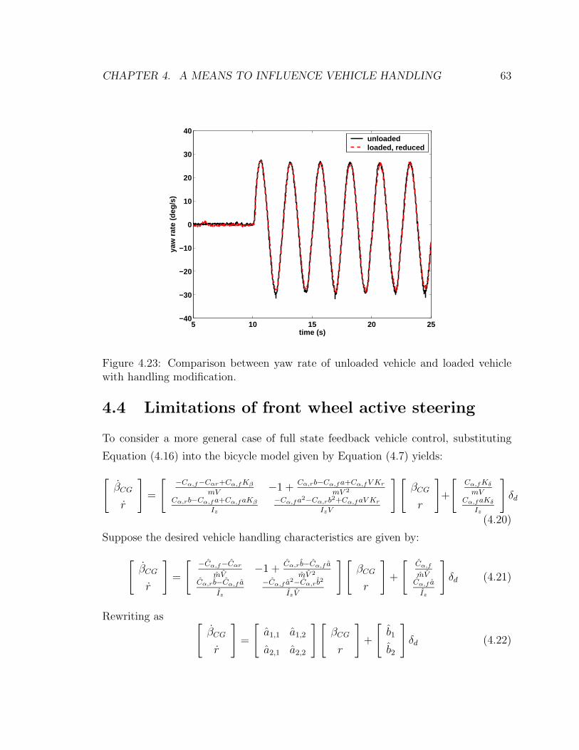
CHAPTER 4. A MEANS TO INFLUENCE VEHICLE HANDLING 63
5 10 15 20 25−40
−30
−20
−10
0
10
20
30
40
time (s)
yaw
rat
e (d
eg/s
)
unloadedloaded, reduced
Figure 4.23: Comparison between yaw rate of unloaded vehicle and loaded vehiclewith handling modification.
4.4 Limitations of front wheel active steering
To consider a more general case of full state feedback vehicle control, substituting
Equation (4.16) into the bicycle model given by Equation (4.7) yields:
[
βCG
r
]
=
[
−Cα,f−Cαr+Cα,f Kβ
mV−1 +
Cα,rb−Cα,f a+Cα,f V Kr
mV 2
Cα,rb−Cα,f a+Cα,f aKβ
Iz
−Cα,f a2−Cα,rb2+Cα,f aV Kr
IzV
][
βCG
r
]
+
[
Cα,f Kδ
mVCα,f aKδ
Iz
]
δd
(4.20)
Suppose the desired vehicle handling characteristics are given by:
[
βCG
r
]
=
[
−Cα,f−Cαr
mV−1 +
Cα,r b−Cα,f a
mV 2
Cα,r b−Cα,f a
Iz
−Cα,f a2−Cα,r b2
IzV
][
βCG
r
]
+
[
Cα,f
mVCα,f a
Iz
]
δd (4.21)
Rewriting as[
βCG
r
]
=
[
a1,1 a1,2
a2,1 a2,2
] [
βCG
r
]
+
[
b1
b2
]
δd (4.22)
CHAPTER 4. A MEANS TO INFLUENCE VEHICLE HANDLING 64
and equating with Equation (4.20),
Cα,f
mVKβ −
Cα,f + Cα,r
mV= a1,1 (4.23)
Cα,f
mVKr +
Cα,r − Cα,f
mV 2− 1 = a1,2 (4.24)
Cα,fa
Iz
Kβ +Cα,rb − Cα,fa
Iz
= a2,1 (4.25)
Cα,fa
Iz
Kr −Cα,fa
2 + Cα,rb2
IzV= a2,2 (4.26)
Cα,fKδ
mV= b1 (4.27)
Cα,faKδ
Iz
= b2 (4.28)
the full state feedback gains, Kβ, Kr, and Kδ, can be expressed in terms of the desired
parameters, a1,1, a1,2, a2,1, and a2,2:
Kβ =mV
Cα,f
a1,1 +Cα,f + Cα,r
Cα,f
(4.29)
Kr =mV
Cα,f
a1,2 +Cα,f − Cα,r + mV 2
Cα,fV(4.30)
Kβ =Iz
Cα,faa2,1 +
Cα,fa − Cα,rb
Cα,fa(4.31)
Kr =Iz
Cα,faa2,2 +
Cα,fa2 + Cα,rb
2
Cα,fV a(4.32)
Kδ =mV
Cα,f
b1 (4.33)
Kδ =Iz
Cα,fab2 (4.34)
CHAPTER 4. A MEANS TO INFLUENCE VEHICLE HANDLING 65
However, since there are more equations than unknowns, the desired parameters
cannot be chosen arbitrarily:
a2,1 =mV a
Iz
a1,1 +Cα,r(a + b)
Iz
(4.35)
a2,2 =mV a
Iz
a1,2 +Cα,f (1 − a2) − Cα,r(1 + b2) + mV 2
IzV(4.36)
b2 =mV a
Iz
b1 (4.37)
The choice of modifying front tire cornering stiffness falls naturally from this deriva-
tion because of the way the cornering stiffness parameter interacts with both front
steer angle and the vehicle dynamics. Other choices are possible, but they do not
carry the physical meaning and significance of modifying a single physical parameter.
Given four-wheel steering capability, however, the range of modifiable parameters
expands to rear cornering stiffness, mass, and moment of inertia (see Appendix C).
While the idea of a variable dynamics vehicle has been considered before [42, 27],
to the best of the author’s knowledge this work represents the first successful im-
plementation of true handling characteristic modification on an actual test vehicle.
Two developments make it possible: precise active steering capability provided by
the steer-by-wire system and accurate, smooth, and continuous state feedback from
the GPS/INS system. The combination of these two systems allows a driver to trans-
parently adjust the balance between handling responsiveness and safety by effectively
changing the vehicle’s physical characteristics and therefore its fundamental handling
response. Handling modification is not, however, a guarantee of safety. Preventing
complete loss of handling control requires knowledge of the tire forces at each corner
and how close they are to reaching their limits. The next chapter applies an under-
standing of steering forces toward obtaining this critical piece of information and in
turn developing an alternative method for sideslip estimation.
Chapter 5
A vehicle dynamics state observer
An interesting and very useful connection has emerged between the steering system
dynamics and the vehicle dynamics as they are each transmitted through the tire
forces. Chapter 3 described the tire aligning moment as a disturbance on the steering
system—due to the lateral tire forces acting about the steering axis—that needs to be
cancelled out by the steering controller. Chapter 4 discussed these same lateral tire
forces as functions of the tire slip angles, which are directly related to the vehicle’s
yaw and sideslip motion. If the steering controller is able to determine and cancel
out the aligning moment, then it stands to reason that the same information can be
used to help estimate the lateral tire forces and in turn the tire slip angles. In this
role, not only does the steer-by-wire system serve a means of actuation to control the
vehicle motion, but it also provides the measurements needed to estimate the vehicle
states. As a matter of convenience and cost, steer-by-wire single-handedly addresses
the problems of both vehicle dynamics control and state estimation.
This chapter develops two observer structures based on linear models of the vehicle
and tire behavior to estimate the vehicle states from measurements of steering angle
and yaw rate. Steering angle and yaw rate sensors are both inexpensive and common
to vehicles already equipped with stability control systems. Steering torque sensors
are intrinsic components of electric power steering systems [40]. Furthermore, as
steer-by-wire technology approaches reality, complete knowledge of steering torque
can be determined from the current applied to the electric steering actuator [30]. The
66
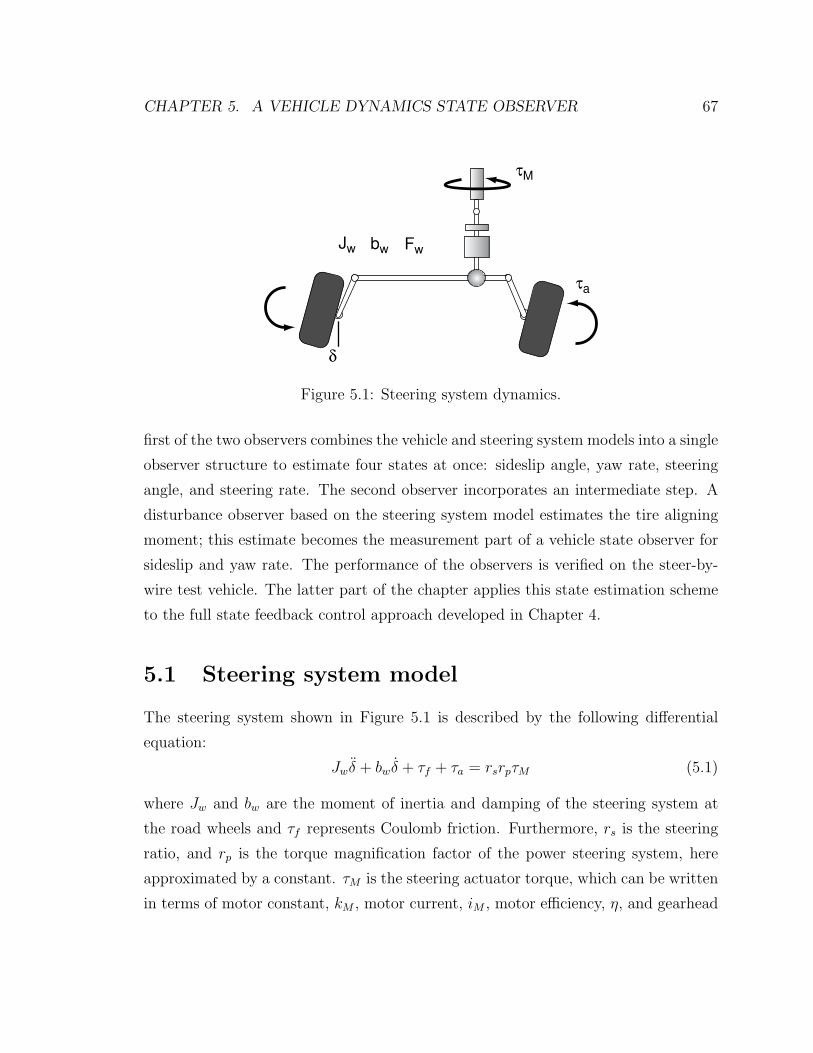
CHAPTER 5. A VEHICLE DYNAMICS STATE OBSERVER 67
Jw bw
τM
δ
τa
Fw
Figure 5.1: Steering system dynamics.
first of the two observers combines the vehicle and steering system models into a single
observer structure to estimate four states at once: sideslip angle, yaw rate, steering
angle, and steering rate. The second observer incorporates an intermediate step. A
disturbance observer based on the steering system model estimates the tire aligning
moment; this estimate becomes the measurement part of a vehicle state observer for
sideslip and yaw rate. The performance of the observers is verified on the steer-by-
wire test vehicle. The latter part of the chapter applies this state estimation scheme
to the full state feedback control approach developed in Chapter 4.
5.1 Steering system model
The steering system shown in Figure 5.1 is described by the following differential
equation:
Jwδ + bwδ + τf + τa = rsrpτM (5.1)
where Jw and bw are the moment of inertia and damping of the steering system at
the road wheels and τf represents Coulomb friction. Furthermore, rs is the steering
ratio, and rp is the torque magnification factor of the power steering system, here
approximated by a constant. τM is the steering actuator torque, which can be written
in terms of motor constant, kM , motor current, iM , motor efficiency, η, and gearhead
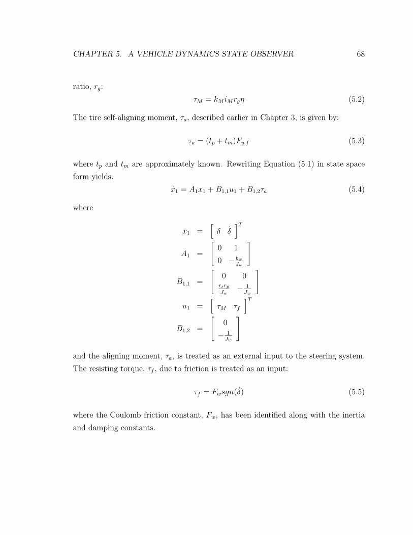
CHAPTER 5. A VEHICLE DYNAMICS STATE OBSERVER 68
ratio, rg:
τM = kM iMrgη (5.2)
The tire self-aligning moment, τa, described earlier in Chapter 3, is given by:
τa = (tp + tm)Fy,f (5.3)
where tp and tm are approximately known. Rewriting Equation (5.1) in state space
form yields:
x1 = A1x1 + B1,1u1 + B1,2τa (5.4)
where
x1 =[
δ δ
]T
A1 =
[
0 1
0 − bw
Jw
]
B1,1 =
[
0 0rsrp
Jw− 1
Jw
]
u1 =[
τM τf
]T
B1,2 =
[
0
− 1
Jw
]
and the aligning moment, τa, is treated as an external input to the steering system.
The resisting torque, τf , due to friction is treated as an input:
τf = Fwsgn(δ) (5.5)
where the Coulomb friction constant, Fw, has been identified along with the inertia
and damping constants.
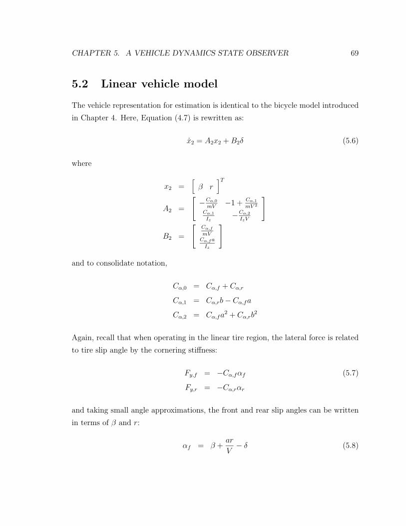
CHAPTER 5. A VEHICLE DYNAMICS STATE OBSERVER 69
5.2 Linear vehicle model
The vehicle representation for estimation is identical to the bicycle model introduced
in Chapter 4. Here, Equation (4.7) is rewritten as:
x2 = A2x2 + B2δ (5.6)
where
x2 =[
β r
]T
A2 =
[
−Cα,0
mV−1 + Cα,1
mV 2
Cα,1
Iz−Cα,2
IzV
]
B2 =
[
Cα,f
mVCα,f a
Iz
]
and to consolidate notation,
Cα,0 = Cα,f + Cα,r
Cα,1 = Cα,rb − Cα,fa
Cα,2 = Cα,fa2 + Cα,rb
2
Again, recall that when operating in the linear tire region, the lateral force is related
to tire slip angle by the cornering stiffness:
Fy,f = −Cα,fαf (5.7)
Fy,r = −Cα,rαr
and taking small angle approximations, the front and rear slip angles can be written
in terms of β and r:
αf = β +ar
V− δ (5.8)
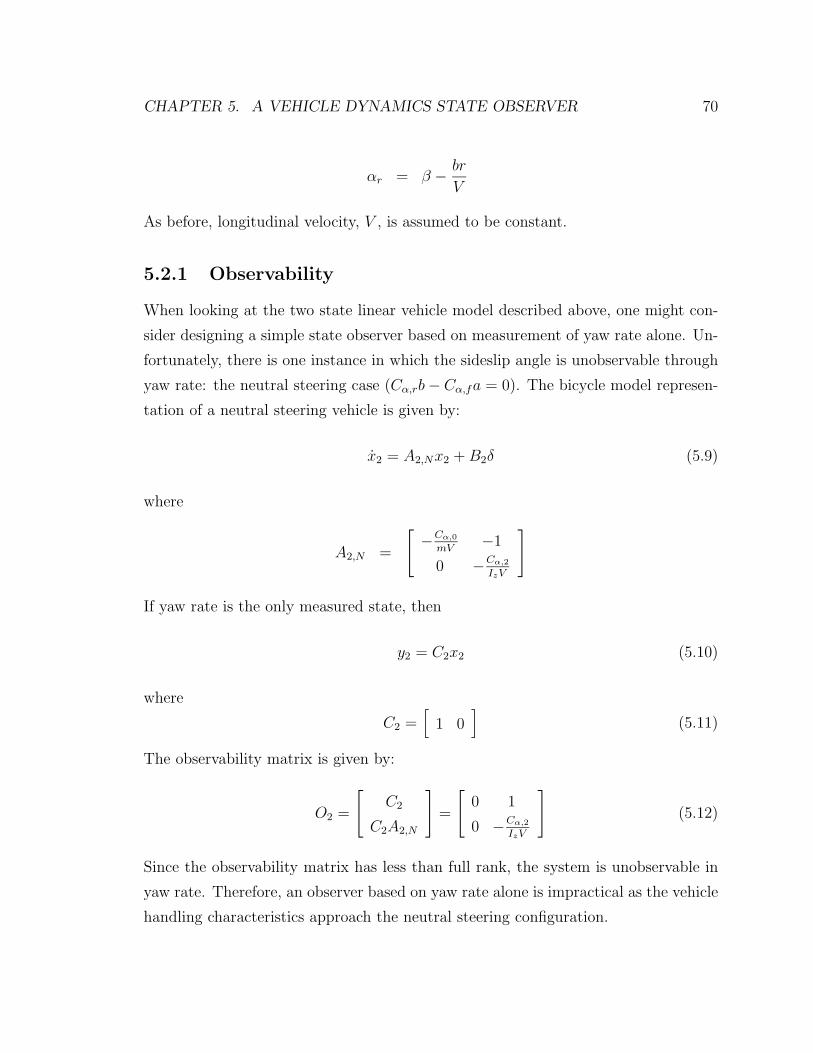
CHAPTER 5. A VEHICLE DYNAMICS STATE OBSERVER 70
αr = β −br
V
As before, longitudinal velocity, V , is assumed to be constant.
5.2.1 Observability
When looking at the two state linear vehicle model described above, one might con-
sider designing a simple state observer based on measurement of yaw rate alone. Un-
fortunately, there is one instance in which the sideslip angle is unobservable through
yaw rate: the neutral steering case (Cα,rb − Cα,fa = 0). The bicycle model represen-
tation of a neutral steering vehicle is given by:
x2 = A2,Nx2 + B2δ (5.9)
where
A2,N =
[
−Cα,0
mV−1
0 −Cα,2
IzV
]
If yaw rate is the only measured state, then
y2 = C2x2 (5.10)
where
C2 =[
1 0]
(5.11)
The observability matrix is given by:
O2 =
[
C2
C2A2,N
]
=
[
0 1
0 −Cα,2
IzV
]
(5.12)
Since the observability matrix has less than full rank, the system is unobservable in
yaw rate. Therefore, an observer based on yaw rate alone is impractical as the vehicle
handling characteristics approach the neutral steering configuration.
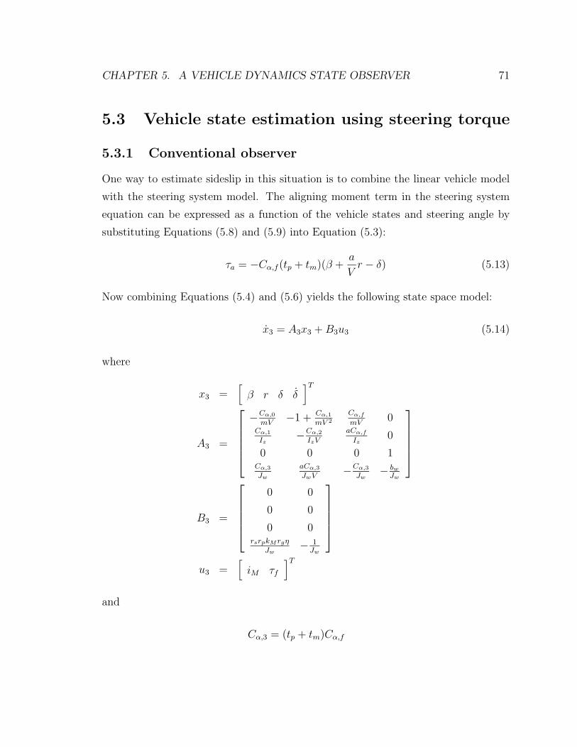
CHAPTER 5. A VEHICLE DYNAMICS STATE OBSERVER 71
5.3 Vehicle state estimation using steering torque
5.3.1 Conventional observer
One way to estimate sideslip in this situation is to combine the linear vehicle model
with the steering system model. The aligning moment term in the steering system
equation can be expressed as a function of the vehicle states and steering angle by
substituting Equations (5.8) and (5.9) into Equation (5.3):
τa = −Cα,f (tp + tm)(β +a
Vr − δ) (5.13)
Now combining Equations (5.4) and (5.6) yields the following state space model:
x3 = A3x3 + B3u3 (5.14)
where
x3 =[
β r δ δ
]T
A3 =
−Cα,0
mV−1 + Cα,1
mV 2
Cα,f
mV0
Cα,1
Iz−Cα,2
IzV
aCα,f
Iz0
0 0 0 1Cα,3
Jw
aCα,3
JwV−Cα,3
Jw− bw
Jw
B3 =
0 0
0 0
0 0rsrpkMrgη
Jw− 1
Jw
u3 =[
iM τf
]T
and
Cα,3 = (tp + tm)Cα,f
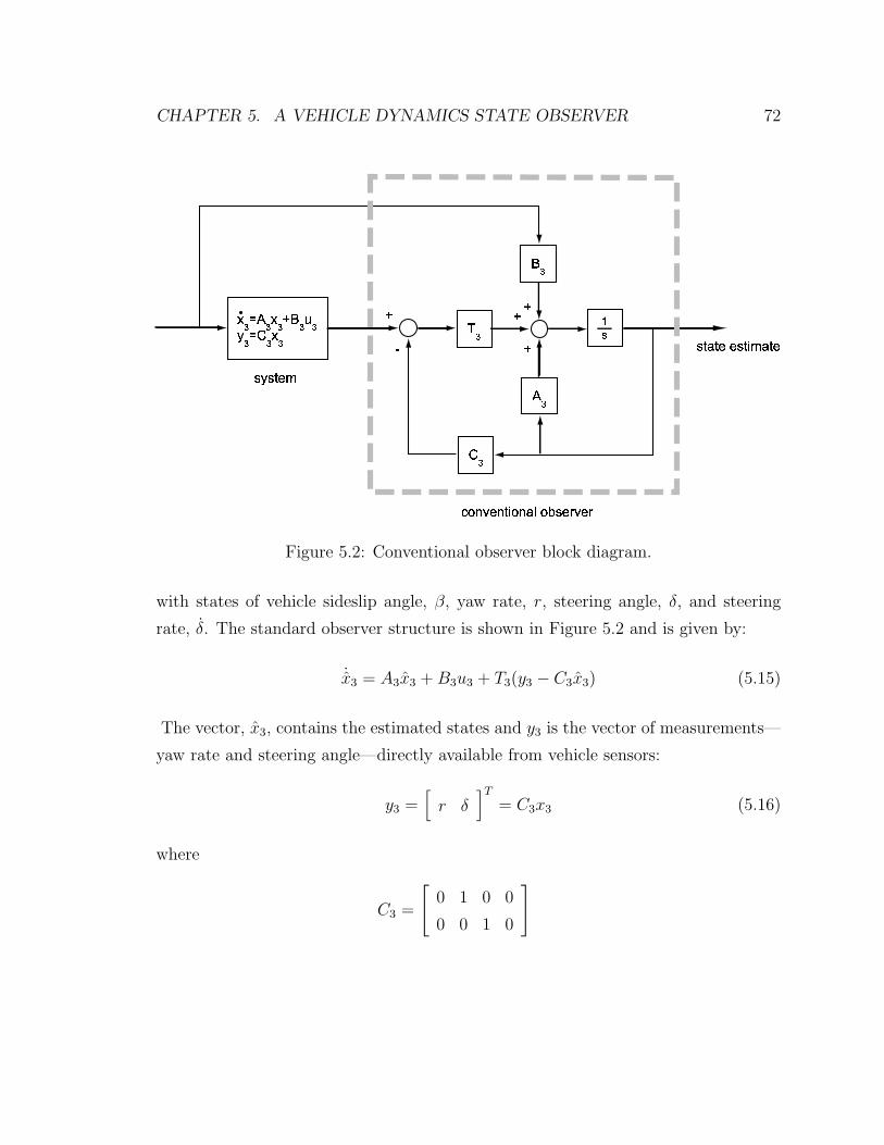
CHAPTER 5. A VEHICLE DYNAMICS STATE OBSERVER 72
9:
;:
<:
=:>
?@?ABC
?ADABB?AECDAB
FGHIBHAEGHDJGK?BLIBL
M:N<:M:O9:P:@:N;:M: QOOO
OR
Figure 5.2: Conventional observer block diagram.
with states of vehicle sideslip angle, β, yaw rate, r, steering angle, δ, and steering
rate, δ. The standard observer structure is shown in Figure 5.2 and is given by:
˙x3 = A3x3 + B3u3 + T3(y3 − C3x3) (5.15)
The vector, x3, contains the estimated states and y3 is the vector of measurements—
yaw rate and steering angle—directly available from vehicle sensors:
y3 =[
r δ
]T
= C3x3 (5.16)
where
C3 =
[
0 1 0 0
0 0 1 0
]
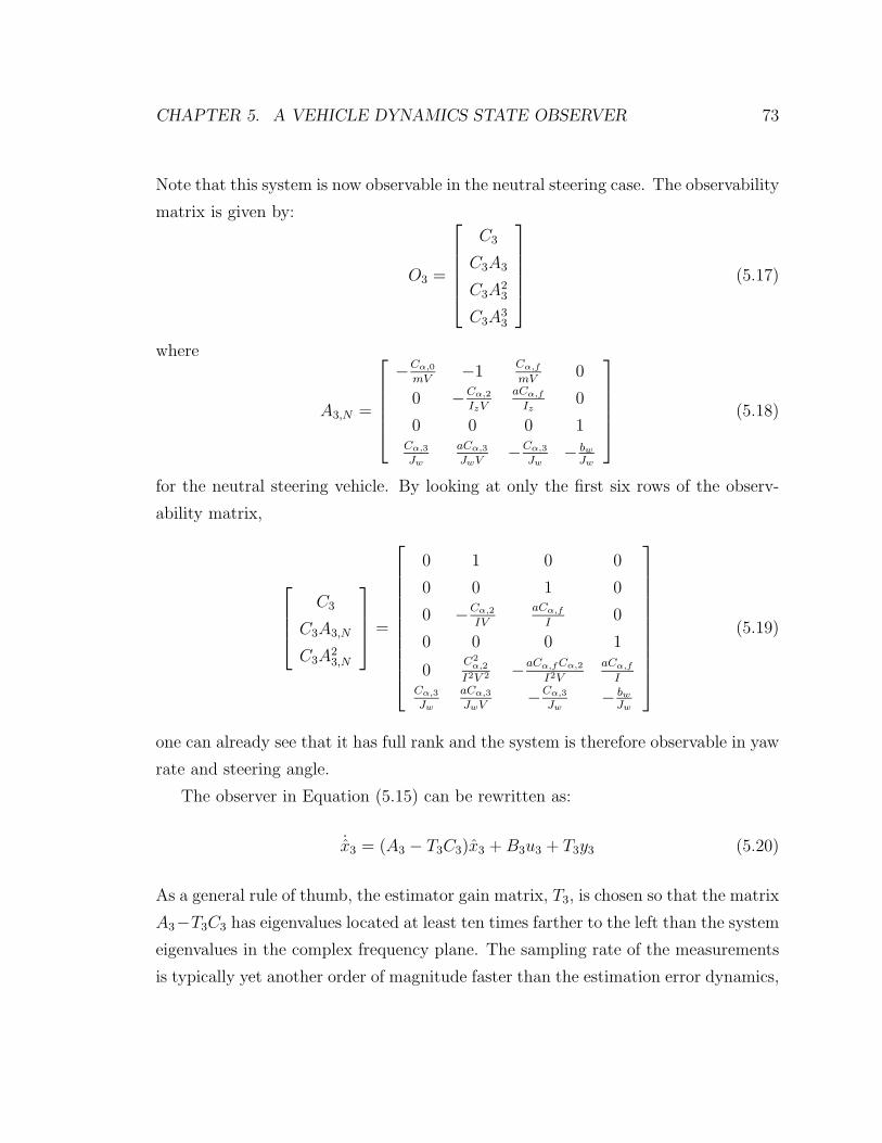
CHAPTER 5. A VEHICLE DYNAMICS STATE OBSERVER 73
Note that this system is now observable in the neutral steering case. The observability
matrix is given by:
O3 =
C3
C3A3
C3A23
C3A33
(5.17)
where
A3,N =
−Cα,0
mV−1
Cα,f
mV0
0 −Cα,2
IzV
aCα,f
Iz0
0 0 0 1Cα,3
Jw
aCα,3
JwV−Cα,3
Jw− bw
Jw
(5.18)
for the neutral steering vehicle. By looking at only the first six rows of the observ-
ability matrix,
C3
C3A3,N
C3A23,N
=
0 1 0 0
0 0 1 0
0 −Cα,2
IV
aCα,f
I0
0 0 0 1
0C2
α,2
I2V 2 −aCα,f Cα,2
I2V
aCα,f
ICα,3
Jw
aCα,3
JwV−Cα,3
Jw− bw
Jw
(5.19)
one can already see that it has full rank and the system is therefore observable in yaw
rate and steering angle.
The observer in Equation (5.15) can be rewritten as:
˙x3 = (A3 − T3C3)x3 + B3u3 + T3y3 (5.20)
As a general rule of thumb, the estimator gain matrix, T3, is chosen so that the matrix
A3−T3C3 has eigenvalues located at least ten times farther to the left than the system
eigenvalues in the complex frequency plane. The sampling rate of the measurements
is typically yet another order of magnitude faster than the estimation error dynamics,
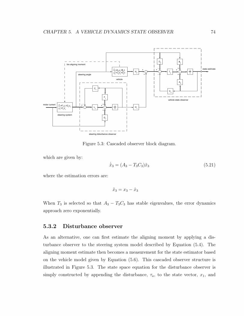
CHAPTER 5. A VEHICLE DYNAMICS STATE OBSERVER 74
z1=F
1z
1+G
1u
1y
1=C
1z
1
G1
C1
F1
L1
1
steering system
steering disturbance observer
s
+ +
+
+-
x2=A
2x
2+B
2δ
y2=C
2x
2+D
2δ
D2
B2
C2
A2
T2
1
vehicle
state estimate
vehicle state observer
s
+ ++
+
-
-
H2
+
+
H1
steering angle
tire aligning moment
motor current
Figure 5.3: Cascaded observer block diagram.
which are given by:
˙x3 = (A3 − T3C3)x3 (5.21)
where the estimation errors are:
x3 = x3 − x3
When T3 is selected so that A3 − T3C3 has stable eigenvalues, the error dynamics
approach zero exponentially.
5.3.2 Disturbance observer
As an alternative, one can first estimate the aligning moment by applying a dis-
turbance observer to the steering system model described by Equation (5.4). The
aligning moment estimate then becomes a measurement for the state estimator based
on the vehicle model given by Equation (5.6). This cascaded observer structure is
illustrated in Figure 5.3. The state space equation for the disturbance observer is
simply constructed by appending the disturbance, τa, to the state vector, x1, and
CHAPTER 5. A VEHICLE DYNAMICS STATE OBSERVER 75
augmenting the corresponding rows in the state matrices with zeroes:
z1 = F1z1 + G1u1 + J1τa (5.22)
where
z1 =[
δ δ τa
]T
F1 =
[
A1 B1,2
0 0
]
G1 =
[
B1,1
0
]
J1 =[
0 0 1]T
The available measurement, y1, is the steering angle, δ:
y1 = δ = C1z1 (5.23)
where
C1 =[
1 0 0]
The disturbance observer is given by:
˙z1 = F1z1 + G1u1 + L1(y1 − C1z1) (5.24)
and the corresponding error dynamics are:
˙z1 = (F1 − L1C1)z1 + J1τa (5.25)
where the estimation errors are:
z1 = z1 − z1
CHAPTER 5. A VEHICLE DYNAMICS STATE OBSERVER 76
As can be seen from Equation (5.25), the estimation errors do not necessarily approach
zero due to the term containing the derivative of disturbance torque. However, this
term is small if the disturbance is varying slowly. Making the assumption that τa
equals zero is similar to the approach taken in [57] and results in a close approximation
of the disturbance torque from the observer.
5.3.3 Vehicle state observer
Now the standard observer structure is applied to Equation (5.6) only:
˙x2 = A2x2 + B2δ + T2(y2 − y2) (5.26)
This can be rewritten as:
˙x2 = A2,1z1 + A2,2x2 + T2(y2 − C2x2 − D2C1z1) (5.27)
where
A2,1 =[
B2 0 0]
A2,2 = A2
The vector, x2, contains the vehicle states to be estimated and y2 is the vector of
“measurements”—in this case, yaw rate and the aligning moment estimate obtained
from the disturbance observer:
y2 = H2x2 + H1z1 (5.28)
where
H1 =
[
0 0 0
0 0 1
]
H2 =
[
0 1
0 0
]
CHAPTER 5. A VEHICLE DYNAMICS STATE OBSERVER 77
Recall that substituting Equations (5.8), (5.9) and (5.2) into Equation (5.1) expresses
the aligning moment, τa, in terms of the vehicle states, β and r, so that the measure-
ment vector can also be written as:
y2 =[
r τa
]T
= C2x2 + D2δ (5.29)
where
C2 =
[
0 1
−Cα,3 −aCα,3
V
]
D2 =
[
0
Cα,3
]
While Equation (5.6) is unobservable in the neutral steering case when yaw rate, r,
is the sole measurement, the addition of aligning moment, τa, to the measurement
vector means that the system given by Equations (5.6) and (5.29) will always be
observable. Due to the cascaded structure of the observer, the error dynamics here
depend on both the disturbance estimation errors and the vehicle state estimation
errors:
˙x2 = (A2,1 − T2D2C1)z1 + (A2,2 − T2C2)x2 (5.30)
where the estimation errors are:
z1 = z1 − z1
x2 = x2 − x2
5.3.4 Alternate formulation
As mentioned in the previous section, a more technically accurate formulation of the
disturbance observer should include the derivative of the disturbance as a function of
the steering rate as well as the dynamics of the vehicle:
τa = −Cα,f (tp + tm)(β +a
Vr − δ) (5.31)
CHAPTER 5. A VEHICLE DYNAMICS STATE OBSERVER 78
Now β and r can be replaced by the results from the vehicle state observer of Equation
(5.27):
β = −Cα,0
mVβ +
(
−1 +Cα,1
mV 2
)
r +Cα,f
mVδ (5.32)
r = −Cα,1
Iz
β −Cα,2
IzVr +
aCα,f
Iz
δ
The state space equations for the disturbance observer are alternatively written as:
z1 = F2,1z1 + F2,2x2 + G1u1 (5.33)
where
F2,1 =
0 1 0
0 − bw
Jw− 1
Jw
−Cα,3
(
Cα,f
mV+
a2Cα,f
IzV
)
Cα,3 0
F2,2 =
0 0
0 0
Cα,3
(
Cα,0
mV+ Cα,1
Iz
)
Cα,3
(
1 − Cα,1
mV+ aCα,2
IzV 2
)
The available measurement, y1, is the same as before. The disturbance observer for
the alternate formulation is given by:
˙z1 = F2,1z1 + F2,2x2 + G1u1 + L2(y1 − C1z1) (5.34)
and the corresponding error dynamics are:
˙z1 = (F2,1 − L2C1)z1 + F2,2x2 (5.35)
Combining the error dynamics of the disturbance observer with those of the vehicle
state observer, Equation (5.30), yields the overall error dynamics for the complete
CHAPTER 5. A VEHICLE DYNAMICS STATE OBSERVER 79
cascaded observer structure:
[
˙z1
˙x2
]
=
[
F2,1 − L2C1 F2,2
A2,1 − T2D2C1 A2,2 − T2C2
][
z1
x2
]
(5.36)
As before, the appropriate choice of observer gain matrices, L2 and T2, will ensure
that the estimation errors, z1 and x2, approach zero exponentially.
While the cascaded observer has many similarities to the conventional observer
described by Equation (5.15), the error dynamics clearly illustrate a fundamental dif-
ference between the two approaches. In the formulation of the conventional observer,
the existence of aligning moment is implied through the merging of the steering sys-
tem and vehicle into a single entity. In the cascaded observer, the separation of
the steering system dynamics and vehicle dynamics is more distinct. By explicitly
bringing out the aligning moment as a state to be observed, the cascaded structure
emphasizes the intermediary role aligning moment plays in going from steering torque
measurement to vehicle state estimates. Although both observer types are designed
to estimate the vehicle states, the structural differences suggest that they will not
perform in exactly the same way.
5.3.5 Observer performance
Both the conventional observer and the cascaded observer structure with the sim-
plified disturbance observer have been implemented in real-time on the steer-by-wire
test vehicle. The state estimates from the observers are simultaneously compared to
results from the GPS/INS based sideslip estimation method described in Chapter 4.
As a reference, vehicle states calculated from the linear vehicle model—with parame-
ters matched to the test vehicle—are also included in the comparison. The following
figures correspond to the same test cycle during which the vehicle accelerates from
a standing stop to a steady speed of 6.7 m/s (15 mi/hr) at which time the steering
maneuver is initiated.
Figures 5.4, 5.5, 5.6, and 5.7 show the state estimates from the four-state observer.
As expected, since steering angle and yaw rate are measurements, the estimates of
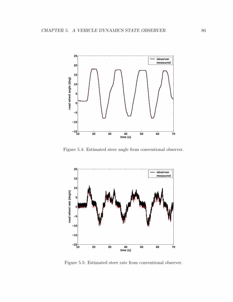
CHAPTER 5. A VEHICLE DYNAMICS STATE OBSERVER 80
10 20 30 40 50 60 70−15
−10
−5
0
5
10
15
20
25
time (s)
road
whe
el a
ngle
(de
g)
observermeasured
Figure 5.4: Estimated steer angle from conventional observer.
10 20 30 40 50 60 70−20
−15
−10
−5
0
5
10
15
20
time (s)
road
whe
el r
ate
(deg
/s)
observermeasured
Figure 5.5: Estimated steer rate from conventional observer.
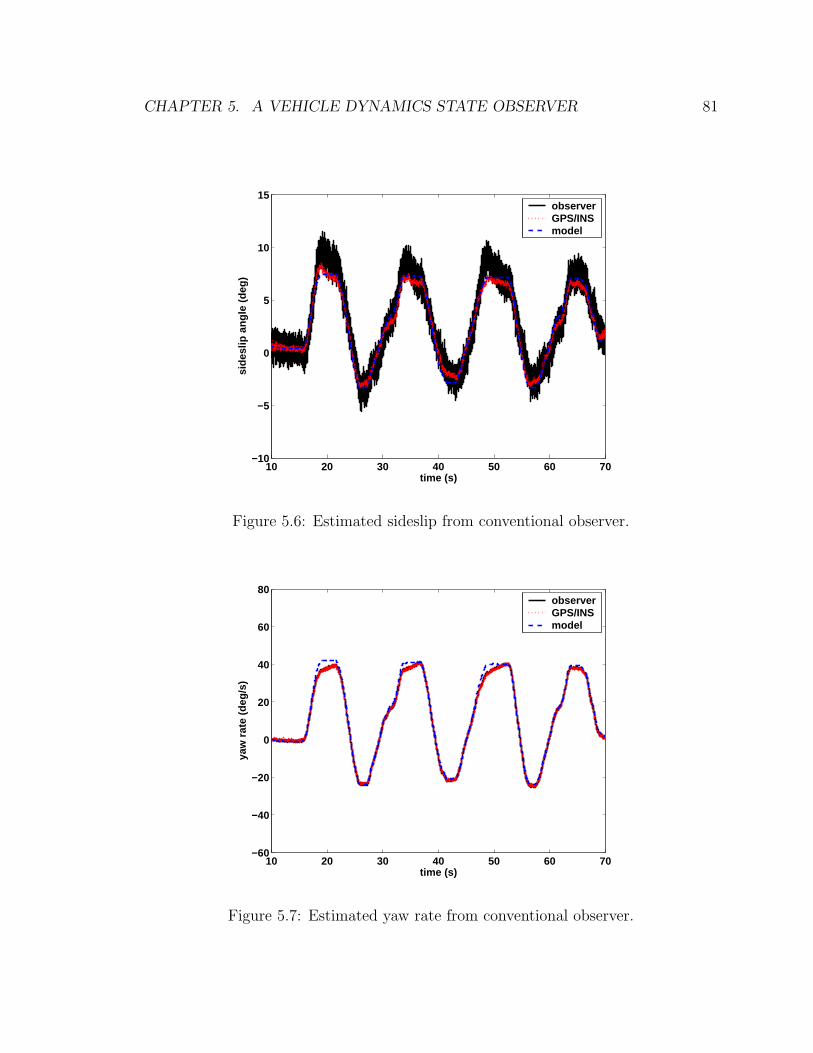
CHAPTER 5. A VEHICLE DYNAMICS STATE OBSERVER 81
10 20 30 40 50 60 70−10
−5
0
5
10
15
time (s)
side
slip
ang
le (
deg)
observerGPS/INSmodel
Figure 5.6: Estimated sideslip from conventional observer.
10 20 30 40 50 60 70−60
−40
−20
0
20
40
60
80
time (s)
yaw
rat
e (d
eg/s
)
observerGPS/INSmodel
Figure 5.7: Estimated yaw rate from conventional observer.
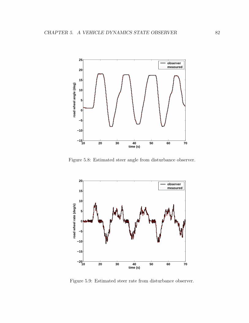
CHAPTER 5. A VEHICLE DYNAMICS STATE OBSERVER 82
10 20 30 40 50 60 70−15
−10
−5
0
5
10
15
20
25
time (s)
road
whe
el a
ngle
(de
g)
observermeasured
Figure 5.8: Estimated steer angle from disturbance observer.
10 20 30 40 50 60 70−20
−15
−10
−5
0
5
10
15
20
time (s)
road
whe
el r
ate
(deg
/s)
observermeasured
Figure 5.9: Estimated steer rate from disturbance observer.
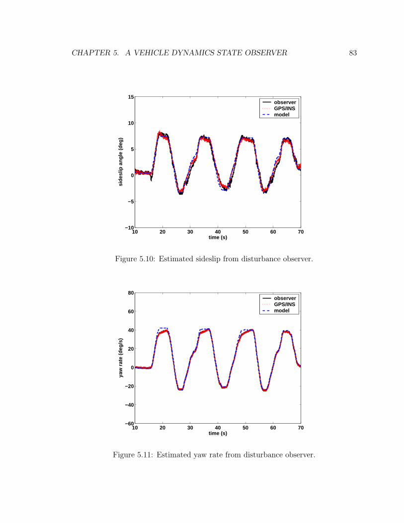
CHAPTER 5. A VEHICLE DYNAMICS STATE OBSERVER 83
10 20 30 40 50 60 70−10
−5
0
5
10
15
time (s)
side
slip
ang
le (
deg)
observerGPS/INSmodel
Figure 5.10: Estimated sideslip from disturbance observer.
10 20 30 40 50 60 70−60
−40
−20
0
20
40
60
80
time (s)
yaw
rat
e (d
eg/s
)
observerGPS/INSmodel
Figure 5.11: Estimated yaw rate from disturbance observer.
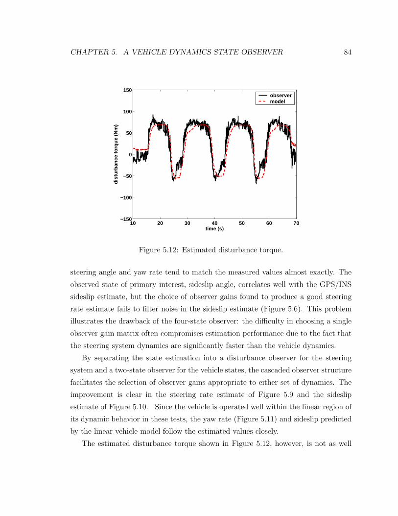
CHAPTER 5. A VEHICLE DYNAMICS STATE OBSERVER 84
10 20 30 40 50 60 70−150
−100
−50
0
50
100
150
time (s)
dist
urba
nce
torq
ue (
Nm
)
observermodel
Figure 5.12: Estimated disturbance torque.
steering angle and yaw rate tend to match the measured values almost exactly. The
observed state of primary interest, sideslip angle, correlates well with the GPS/INS
sideslip estimate, but the choice of observer gains found to produce a good steering
rate estimate fails to filter noise in the sideslip estimate (Figure 5.6). This problem
illustrates the drawback of the four-state observer: the difficulty in choosing a single
observer gain matrix often compromises estimation performance due to the fact that
the steering system dynamics are significantly faster than the vehicle dynamics.
By separating the state estimation into a disturbance observer for the steering
system and a two-state observer for the vehicle states, the cascaded observer structure
facilitates the selection of observer gains appropriate to either set of dynamics. The
improvement is clear in the steering rate estimate of Figure 5.9 and the sideslip
estimate of Figure 5.10. Since the vehicle is operated well within the linear region of
its dynamic behavior in these tests, the yaw rate (Figure 5.11) and sideslip predicted
by the linear vehicle model follow the estimated values closely.
The estimated disturbance torque shown in Figure 5.12, however, is not as well
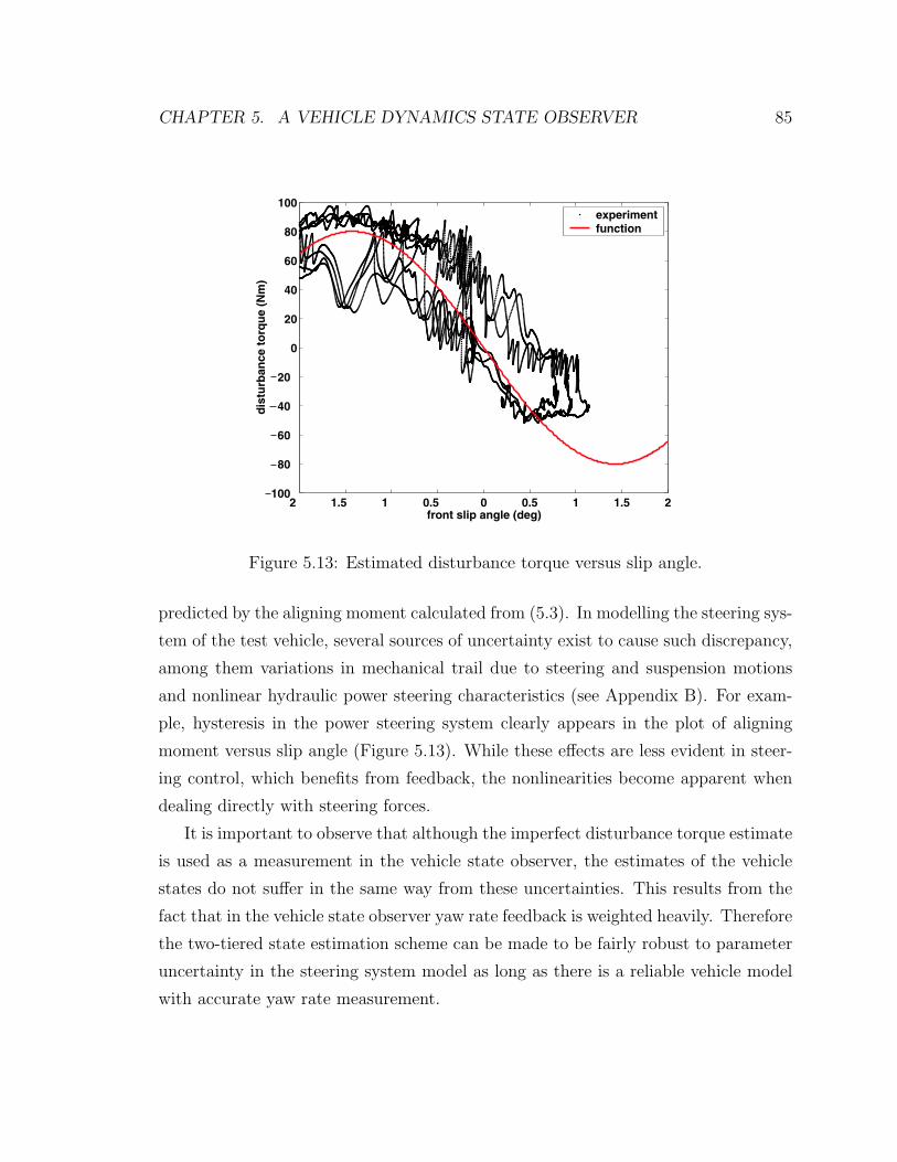
CHAPTER 5. A VEHICLE DYNAMICS STATE OBSERVER 85
2 1.5 1 0.5 0 0.5 1 1.5 2100
80
60
40
20
0
20
40
60
80
100
front slip angle (deg)
dis
turb
an
ce
to
rqu
e (
Nm
)
experimentfunction
Figure 5.13: Estimated disturbance torque versus slip angle.
predicted by the aligning moment calculated from (5.3). In modelling the steering sys-
tem of the test vehicle, several sources of uncertainty exist to cause such discrepancy,
among them variations in mechanical trail due to steering and suspension motions
and nonlinear hydraulic power steering characteristics (see Appendix B). For exam-
ple, hysteresis in the power steering system clearly appears in the plot of aligning
moment versus slip angle (Figure 5.13). While these effects are less evident in steer-
ing control, which benefits from feedback, the nonlinearities become apparent when
dealing directly with steering forces.
It is important to observe that although the imperfect disturbance torque estimate
is used as a measurement in the vehicle state observer, the estimates of the vehicle
states do not suffer in the same way from these uncertainties. This results from the
fact that in the vehicle state observer yaw rate feedback is weighted heavily. Therefore
the two-tiered state estimation scheme can be made to be fairly robust to parameter
uncertainty in the steering system model as long as there is a reliable vehicle model
with accurate yaw rate measurement.
CHAPTER 5. A VEHICLE DYNAMICS STATE OBSERVER 86
5.4 Closed loop vehicle control
5.4.1 Handling modification
The same closed loop handling modification technique introduced in Chapter 4 is
now repeated with state estimates obtained from the disturbance observer method
instead of the GPS/INS system. These tests determine whether the observer-based
state estimation is suitable for use as feedback in a closed loop vehicle control system.
The full state feedback control law for an active steering vehicle is given again by:
δ = Krr + Kββ + Kdδd (5.37)
where δd is the driver commanded steer angle and δ is the augmented angle. Now β
comes from the observer of Equation (5.27). The modified front cornering stiffness is
again defined by:
Cα,f = Cα,f (1 + η) (5.38)
and the state feedback gains as:
Kβ = −η Kr = −a
Vη Kd = (1 + η) (5.39)
Substituting the feedback law, Equation (5.37), into Equation (5.6) yields a state
space equation of the same form as Equation (5.6) but with the new cornering stiffness
Cα,f :
x2 = A2x2 + B2δ (5.40)
where
x2 =[
β r
]T
A2 =
[
− Cα,0
mV−1 + Cα,1
mV 2
Cα,1
Iz− Cα,2
IzV
]
B2 =
[
Cα,f
mVCα,f a
Iz
]
CHAPTER 5. A VEHICLE DYNAMICS STATE OBSERVER 87
and to consolidate notation,
Cα,0 = Cα,f + Cα,r
Cα,1 = Cα,rb − Cα,fa
Cα,2 = Cα,fa2 + Cα,rb
2
5.4.2 Experimental results
As developed thus far in this chapter, all of the components necessary for physical
implementation of closed loop vehicle dynamics control are now in place: 1) accurate
state estimates are available from the disturbance observer described in the previous
section, 2) a means of precise vehicle control is provided by the steer-by-wire system
in the test vehicle, and 3) a full state feedback control law has been devised to funda-
mentally alter a vehicle’s handling characteristics. The experimental results presented
below are based on the same test procedure described in Chapter 4. From the first test
run, with the vehicle driven in the unmodified mode (no state feedback), Figures 5.14
and 5.15) show the plots of yaw rate and sideslip angle. The estimated values from
the disturbance observer are compared with both GPS/INS measurement and bicycle
model simulation. Yaw rate estimated from the disturbance observer matches the
GPS/INS numbers almost exactly since it is the “measured” state by which the ob-
server determines the unmeasurable state of sideslip angle. More importantly, sideslip
angle estimated from the disturbance observer also closely follows GPS measurement
and model prediction.
Next, the same test is repeated with the effective front cornering stiffness reduced
by 50%. Figure 5.16 shows how steering angle has been changed by the state feed-
back so as to exactly replicate the dynamic effect of reduced front cornering stiffness.
The resulting difference in handling behavior is evident when comparing lateral ac-
celeration (Figure 5.17) to the nominal case. As expected, the modified handling
exhibits lower peak lateral acceleration values since the effect of reduced front cor-
nering stiffness is more pronounced understeering behavior. Figures 5.18 and 5.19
confirm that results for the reduced case match simulation of the bicycle model with
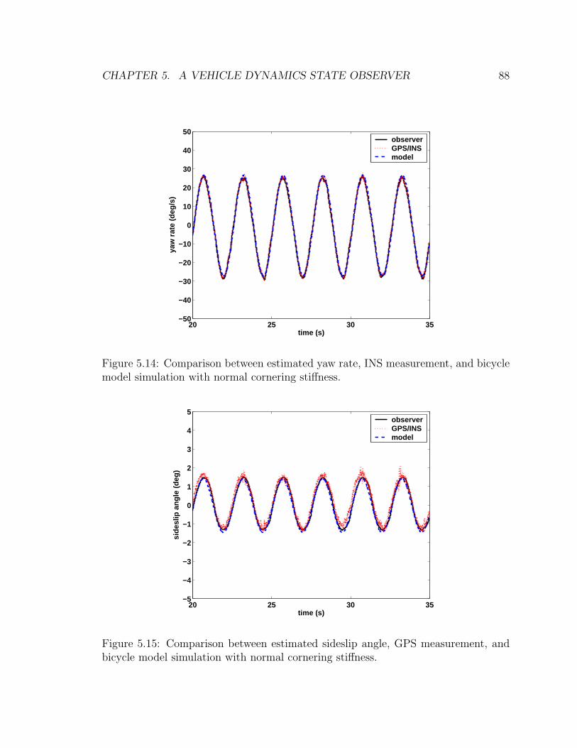
CHAPTER 5. A VEHICLE DYNAMICS STATE OBSERVER 88
20 25 30 35−50
−40
−30
−20
−10
0
10
20
30
40
50
time (s)
yaw
rat
e (d
eg/s
)
observerGPS/INSmodel
Figure 5.14: Comparison between estimated yaw rate, INS measurement, and bicyclemodel simulation with normal cornering stiffness.
20 25 30 35−5
−4
−3
−2
−1
0
1
2
3
4
5
time (s)
side
slip
ang
le (
deg)
observerGPS/INSmodel
Figure 5.15: Comparison between estimated sideslip angle, GPS measurement, andbicycle model simulation with normal cornering stiffness.
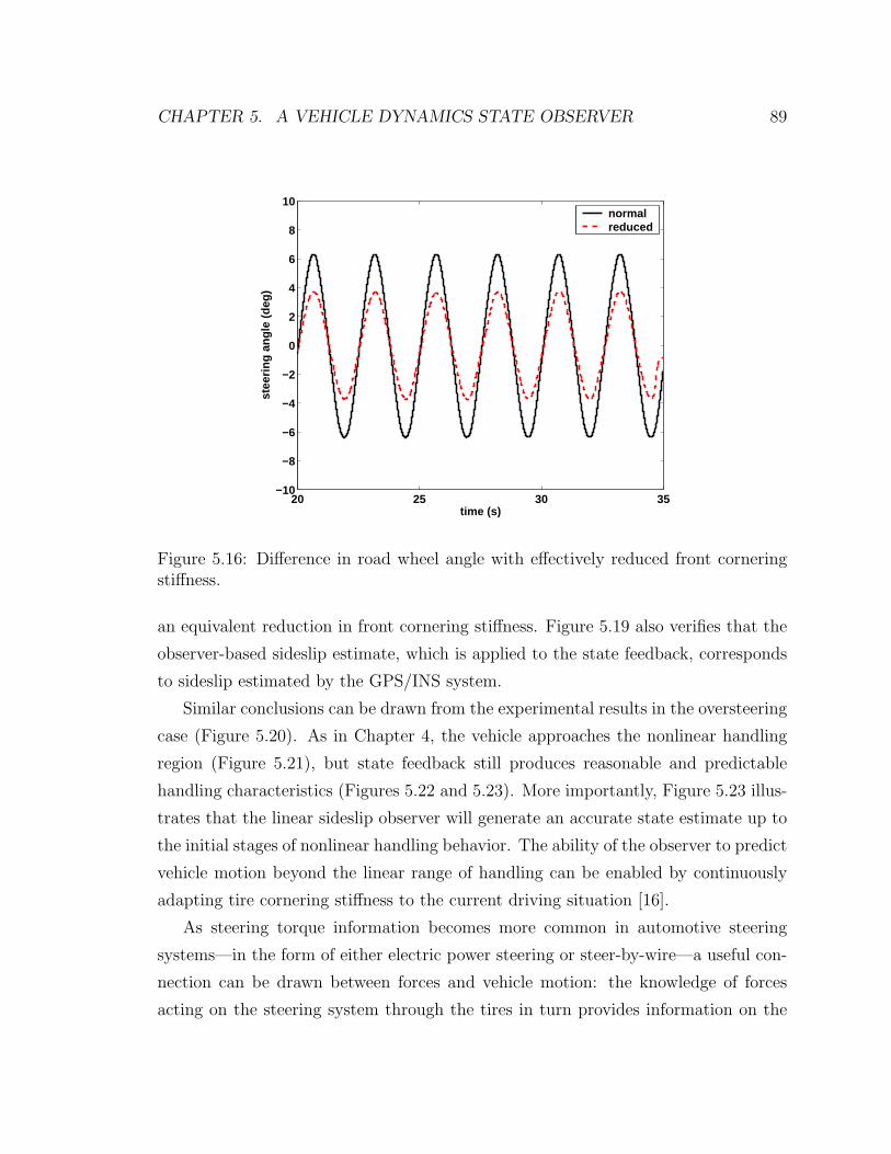
CHAPTER 5. A VEHICLE DYNAMICS STATE OBSERVER 89
20 25 30 35−10
−8
−6
−4
−2
0
2
4
6
8
10
time (s)
stee
ring
angl
e (d
eg)
normalreduced
Figure 5.16: Difference in road wheel angle with effectively reduced front corneringstiffness.
an equivalent reduction in front cornering stiffness. Figure 5.19 also verifies that the
observer-based sideslip estimate, which is applied to the state feedback, corresponds
to sideslip estimated by the GPS/INS system.
Similar conclusions can be drawn from the experimental results in the oversteering
case (Figure 5.20). As in Chapter 4, the vehicle approaches the nonlinear handling
region (Figure 5.21), but state feedback still produces reasonable and predictable
handling characteristics (Figures 5.22 and 5.23). More importantly, Figure 5.23 illus-
trates that the linear sideslip observer will generate an accurate state estimate up to
the initial stages of nonlinear handling behavior. The ability of the observer to predict
vehicle motion beyond the linear range of handling can be enabled by continuously
adapting tire cornering stiffness to the current driving situation [16].
As steering torque information becomes more common in automotive steering
systems—in the form of either electric power steering or steer-by-wire—a useful con-
nection can be drawn between forces and vehicle motion: the knowledge of forces
acting on the steering system through the tires in turn provides information on the
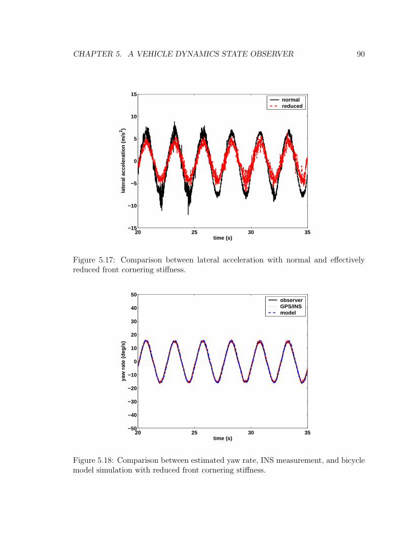
CHAPTER 5. A VEHICLE DYNAMICS STATE OBSERVER 90
20 25 30 35−15
−10
−5
0
5
10
15
time (s)
late
ral a
ccel
erat
ion
(m/s
2 )
normalreduced
Figure 5.17: Comparison between lateral acceleration with normal and effectivelyreduced front cornering stiffness.
20 25 30 35−50
−40
−30
−20
−10
0
10
20
30
40
50
time (s)
yaw
rat
e (d
eg/s
)
observerGPS/INSmodel
Figure 5.18: Comparison between estimated yaw rate, INS measurement, and bicyclemodel simulation with reduced front cornering stiffness.
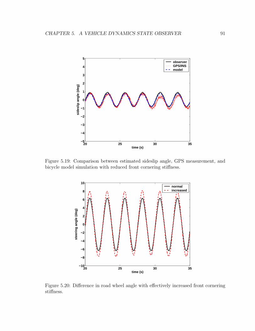
CHAPTER 5. A VEHICLE DYNAMICS STATE OBSERVER 91
20 25 30 35−5
−4
−3
−2
−1
0
1
2
3
4
5
time (s)
side
slip
ang
le (
deg)
observerGPS/INSmodel
Figure 5.19: Comparison between estimated sideslip angle, GPS measurement, andbicycle model simulation with reduced front cornering stiffness.
20 25 30 35−10
−8
−6
−4
−2
0
2
4
6
8
10
time (s)
stee
ring
angl
e (d
eg)
normalincreased
Figure 5.20: Difference in road wheel angle with effectively increased front corneringstiffness.
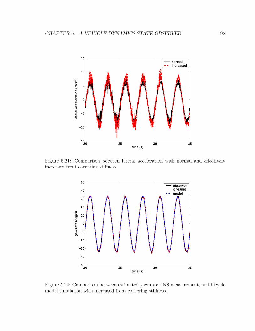
CHAPTER 5. A VEHICLE DYNAMICS STATE OBSERVER 92
20 25 30 35−15
−10
−5
0
5
10
15
time (s)
late
ral a
ccel
erat
ion
(m/s
2 )
normalincreased
Figure 5.21: Comparison between lateral acceleration with normal and effectivelyincreased front cornering stiffness.
20 25 30 35−50
−40
−30
−20
−10
0
10
20
30
40
50
time (s)
yaw
rat
e (d
eg/s
)
observerGPS/INSmodel
Figure 5.22: Comparison between estimated yaw rate, INS measurement, and bicyclemodel simulation with increased front cornering stiffness.
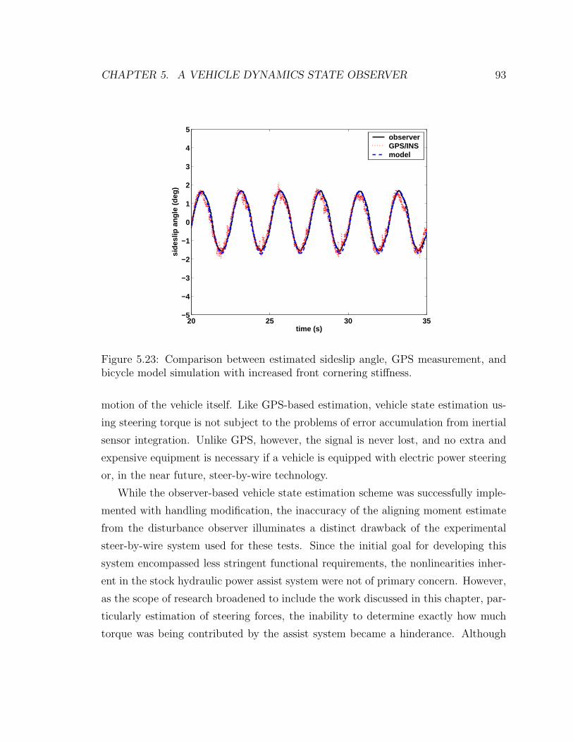
CHAPTER 5. A VEHICLE DYNAMICS STATE OBSERVER 93
20 25 30 35−5
−4
−3
−2
−1
0
1
2
3
4
5
time (s)
side
slip
ang
le (
deg)
observerGPS/INSmodel
Figure 5.23: Comparison between estimated sideslip angle, GPS measurement, andbicycle model simulation with increased front cornering stiffness.
motion of the vehicle itself. Like GPS-based estimation, vehicle state estimation us-
ing steering torque is not subject to the problems of error accumulation from inertial
sensor integration. Unlike GPS, however, the signal is never lost, and no extra and
expensive equipment is necessary if a vehicle is equipped with electric power steering
or, in the near future, steer-by-wire technology.
While the observer-based vehicle state estimation scheme was successfully imple-
mented with handling modification, the inaccuracy of the aligning moment estimate
from the disturbance observer illuminates a distinct drawback of the experimental
steer-by-wire system used for these tests. Since the initial goal for developing this
system encompassed less stringent functional requirements, the nonlinearities inher-
ent in the stock hydraulic power assist system were not of primary concern. However,
as the scope of research broadened to include the work discussed in this chapter, par-
ticularly estimation of steering forces, the inability to determine exactly how much
torque was being contributed by the assist system became a hinderance. Although
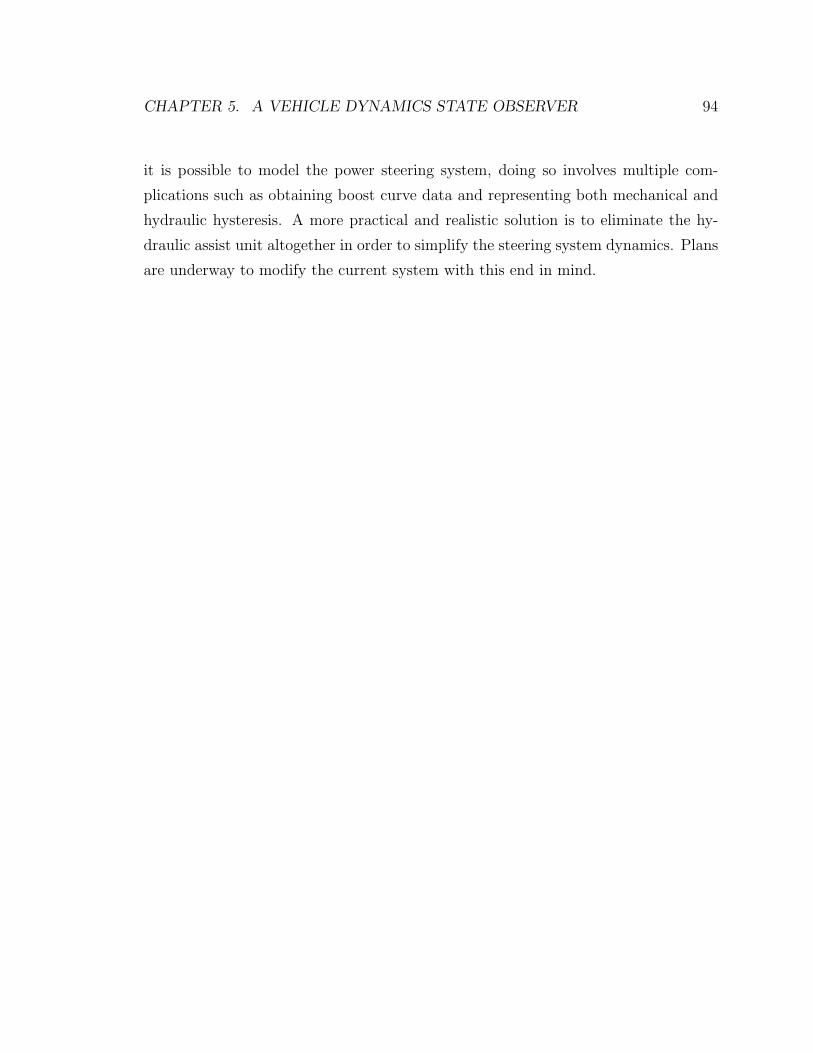
CHAPTER 5. A VEHICLE DYNAMICS STATE OBSERVER 94
it is possible to model the power steering system, doing so involves multiple com-
plications such as obtaining boost curve data and representing both mechanical and
hydraulic hysteresis. A more practical and realistic solution is to eliminate the hy-
draulic assist unit altogether in order to simplify the steering system dynamics. Plans
are underway to modify the current system with this end in mind.
Chapter 6
Conclusion and Future Work
6.1 Conclusion
Given that commercial steer-by-wire systems are many years in the future and there
are still a number of problems that need to be solved, the implementation of by-
wire technology seems like an ideal area for academic research. Since steering is the
primary means by which a driver controls a vehicle’s motion, steer-by-wire opens
many possibilities for investigating advanced steering control algorithms. The flex-
ibility of steer-by-wire serves an entire range of research purposes, from replicating
the driving dynamics of a conventional vehicle [27] to lane-keeping assistance [15] to
fully automated operation [47]. This thesis strives to answer three primary questions
on steer-by-wire: 1) what are the requirements for precise control of a steer-by-wire
system? 2) how can steer-by-wire be used to influence a vehicle’s dynamic character-
istics? and 3) what does steer-by-wire reveal about a vehicle’s dynamic behavior?
In developing an experimental steer-by-wire system, two requirements stand out:
the need to understand the dynamics of the system being controlled and the need to
account for the forces acting on the system during the normal course of operation.
Beginning with a physically-based model, the steering system parameters are obtained
via experimental identification techniques. Feedfoward control is used to cancel out
the system dynamics as well as the disturbance forces attributed to tire aligning
moment. On top of that, feedback control is added to minimize the steering angle error
95
CHAPTER 6. CONCLUSION AND FUTURE WORK 96
due to modelling uncertainties and real nonlinearities. These control techniques form
a general guideline for the design of an accurate and precise steer-by-wire controller.
A vehicle’s handling characteristics are decided by its physical parameters—weight
distribution, tire cornering stiffness, and suspension roll stiffness, to name a few. Nor-
mally, the only way to make a vehicle handle differently is to change one of these
parameters. With active steering capability and vehicle state information, however,
a vehicle’s handling characteristics can indeed be altered even though the vehicle re-
mains physically unmodified. Experimental results show that a vehicle can be made
more oversteering or understeering by artificially adjusting the front tire cornering
stiffness via a combination of precisely controlled steering inputs and full state feed-
back. This represents one of the many safety and performance enhancements possible
with steer-by-wire and also emphasizes the overall need for improved vehicle sensing
and state estimation. To produce good handling responsiveness requires not only
precise steering control but also smooth feedback signals.
One of the most important results involves the unlikely synergy between steer-
ing torque information and sideslip angle estimation. The relation between aligning
moment and lateral tire force allows the combination of the steering system dynam-
ics and vehicle dynamics into a unified observer structure. Consider that only three
types of sensors—steering torque (or steering actuator current), steering angle, and
yaw rate—are needed to generate sideslip angle estimates that can be compared to
estimates obtained from highly accurate measurements by a sophisticated GPS/INS
system. This approach has many practical implications for the next generation of
fully integrated automotive stability control systems with or without steer-by-wire,
since all of the measurement devices necessary for precise vehicle control already exist
and have been inexpensively implemented on production cars.
The research presented in this thesis has answered some fundamental questions
regarding the design of steer-by-wire systems as well as explored the interaction be-
tween steering and vehicle dynamics. By physically separating the act of steering a
vehicle from the vehicle itself, steer-by-wire actually merges the two closer together in
the way they are naturally linked. If there is one lesson to be learned here, it is this:
the more we rely on electronics rather than mechanics, the more we must understand
CHAPTER 6. CONCLUSION AND FUTURE WORK 97
the underlying mechanical principles at work in the system. The transition to by-wire
technology does not simply eliminate the need for mechanical components. We must
instead fill in the missing pieces with knowledge of how the system really functions.
6.2 Future work
The most important question of all is, does steer-by-wire make the car steer better
and more safely? The answer is clearly affirmative, but much remains to be done
toward this regard.
6.2.1 Handling at the limits
Most of the work presented thus far has been based on a linear vehicle model. How-
ever, the most safety critical situations occur near the limits of handling, just before
the tires lose their grip on the road. In a carefully designed steering system, the
aligning moment disturbance effectively communicates the tire forces acting on the
vehicle—regardless of whether it is being operated in the linear or nonlinear handling
region—and thus addresses the limitations of using a linear model-based observer
structure as in Chapter 5. Until now, most approaches to analyzing vehicle dynamics
have focused on measuring vehicle motion—longitudinal speed, yaw rate, lateral ac-
celeration, sideslip angle, and roll angle. Here we have introduced a different way of
thinking about vehicle dynamics that is actually quite basic: forces acting on a rigid
body. If we can measure or estimate all of the forces acting on the vehicle, then we
can completely predict its motion. If we can measure both force and motion, then we
have a way of estimating parameters such as cornering stiffness, particularly in the
nonlinear region of the tire force curve as shown in Figure 6.1 [19].
6.2.2 Steering wheel force feedback
Since a driver gains critical information about the vehicle from feedback through the
steering wheel, steering feel will play a pivotal role in consumer acceptance of steer-
by-wire systems. The desirable sensation of “connectedness” between the steering
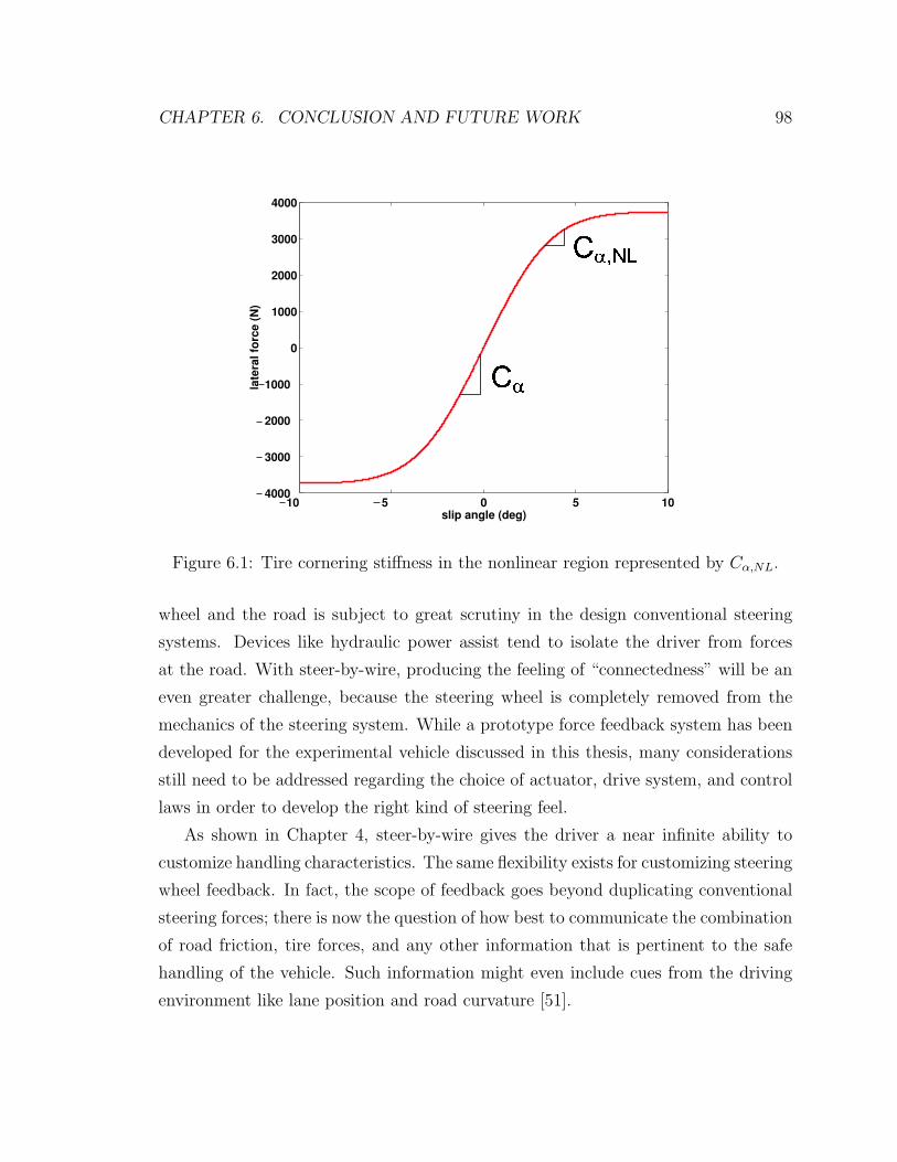
CHAPTER 6. CONCLUSION AND FUTURE WORK 98
10 5 0 5 104000
3000
2000
1000
0
1000
2000
3000
4000
slip angle (deg)
late
ral
forc
e (
N)
ST
STUVW
Figure 6.1: Tire cornering stiffness in the nonlinear region represented by Cα,NL.
wheel and the road is subject to great scrutiny in the design conventional steering
systems. Devices like hydraulic power assist tend to isolate the driver from forces
at the road. With steer-by-wire, producing the feeling of “connectedness” will be an
even greater challenge, because the steering wheel is completely removed from the
mechanics of the steering system. While a prototype force feedback system has been
developed for the experimental vehicle discussed in this thesis, many considerations
still need to be addressed regarding the choice of actuator, drive system, and control
laws in order to develop the right kind of steering feel.
As shown in Chapter 4, steer-by-wire gives the driver a near infinite ability to
customize handling characteristics. The same flexibility exists for customizing steering
wheel feedback. In fact, the scope of feedback goes beyond duplicating conventional
steering forces; there is now the question of how best to communicate the combination
of road friction, tire forces, and any other information that is pertinent to the safe
handling of the vehicle. Such information might even include cues from the driving
environment like lane position and road curvature [51].
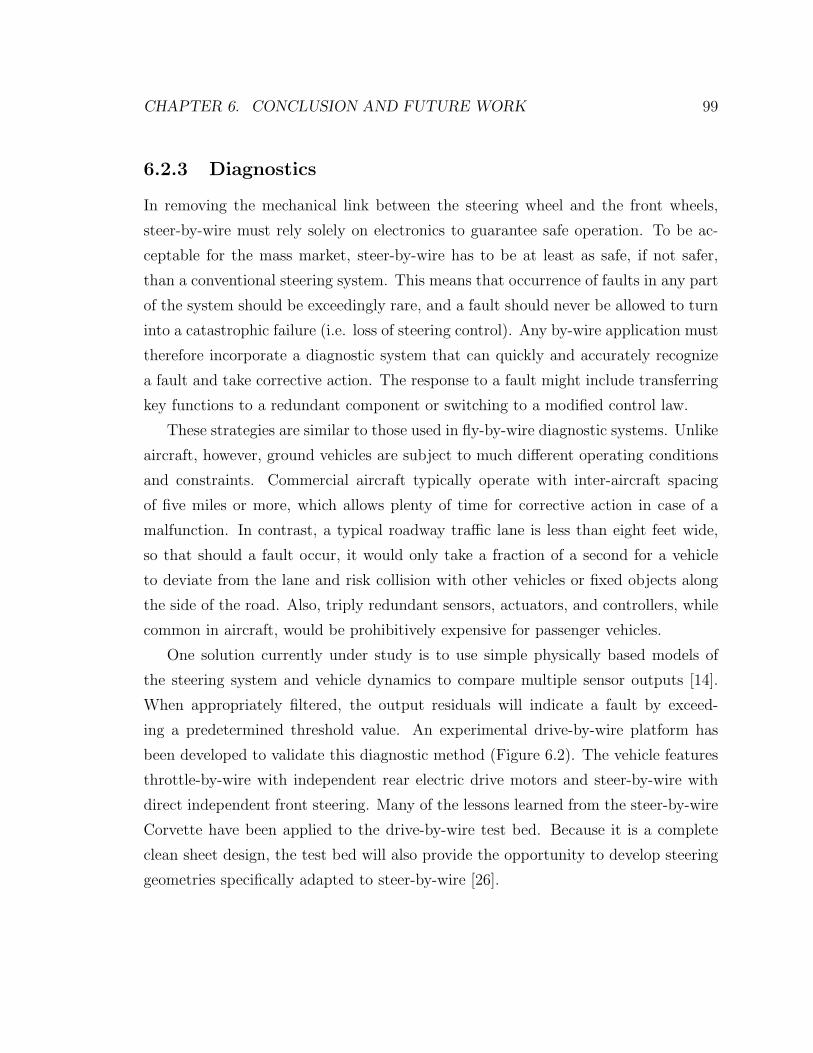
CHAPTER 6. CONCLUSION AND FUTURE WORK 99
6.2.3 Diagnostics
In removing the mechanical link between the steering wheel and the front wheels,
steer-by-wire must rely solely on electronics to guarantee safe operation. To be ac-
ceptable for the mass market, steer-by-wire has to be at least as safe, if not safer,
than a conventional steering system. This means that occurrence of faults in any part
of the system should be exceedingly rare, and a fault should never be allowed to turn
into a catastrophic failure (i.e. loss of steering control). Any by-wire application must
therefore incorporate a diagnostic system that can quickly and accurately recognize
a fault and take corrective action. The response to a fault might include transferring
key functions to a redundant component or switching to a modified control law.
These strategies are similar to those used in fly-by-wire diagnostic systems. Unlike
aircraft, however, ground vehicles are subject to much different operating conditions
and constraints. Commercial aircraft typically operate with inter-aircraft spacing
of five miles or more, which allows plenty of time for corrective action in case of a
malfunction. In contrast, a typical roadway traffic lane is less than eight feet wide,
so that should a fault occur, it would only take a fraction of a second for a vehicle
to deviate from the lane and risk collision with other vehicles or fixed objects along
the side of the road. Also, triply redundant sensors, actuators, and controllers, while
common in aircraft, would be prohibitively expensive for passenger vehicles.
One solution currently under study is to use simple physically based models of
the steering system and vehicle dynamics to compare multiple sensor outputs [14].
When appropriately filtered, the output residuals will indicate a fault by exceed-
ing a predetermined threshold value. An experimental drive-by-wire platform has
been developed to validate this diagnostic method (Figure 6.2). The vehicle features
throttle-by-wire with independent rear electric drive motors and steer-by-wire with
direct independent front steering. Many of the lessons learned from the steer-by-wire
Corvette have been applied to the drive-by-wire test bed. Because it is a complete
clean sheet design, the test bed will also provide the opportunity to develop steering
geometries specifically adapted to steer-by-wire [26].
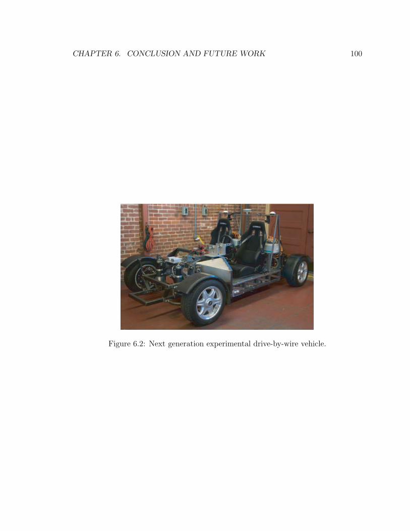
CHAPTER 6. CONCLUSION AND FUTURE WORK 100
Figure 6.2: Next generation experimental drive-by-wire vehicle.
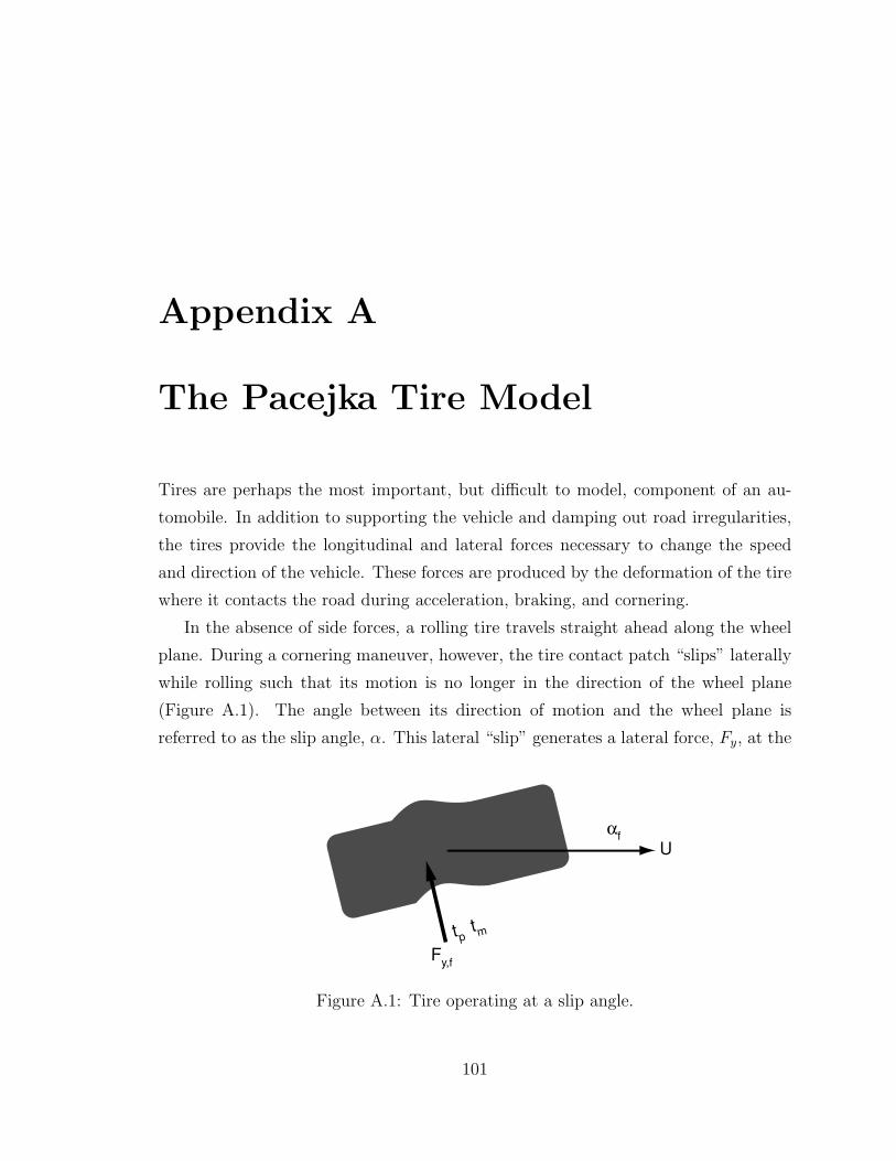
Appendix A
The Pacejka Tire Model
Tires are perhaps the most important, but difficult to model, component of an au-
tomobile. In addition to supporting the vehicle and damping out road irregularities,
the tires provide the longitudinal and lateral forces necessary to change the speed
and direction of the vehicle. These forces are produced by the deformation of the tire
where it contacts the road during acceleration, braking, and cornering.
In the absence of side forces, a rolling tire travels straight ahead along the wheel
plane. During a cornering maneuver, however, the tire contact patch “slips” laterally
while rolling such that its motion is no longer in the direction of the wheel plane
(Figure A.1). The angle between its direction of motion and the wheel plane is
referred to as the slip angle, α. This lateral “slip” generates a lateral force, Fy, at the
tptm
αf
Fy,f
U
Figure A.1: Tire operating at a slip angle.
101
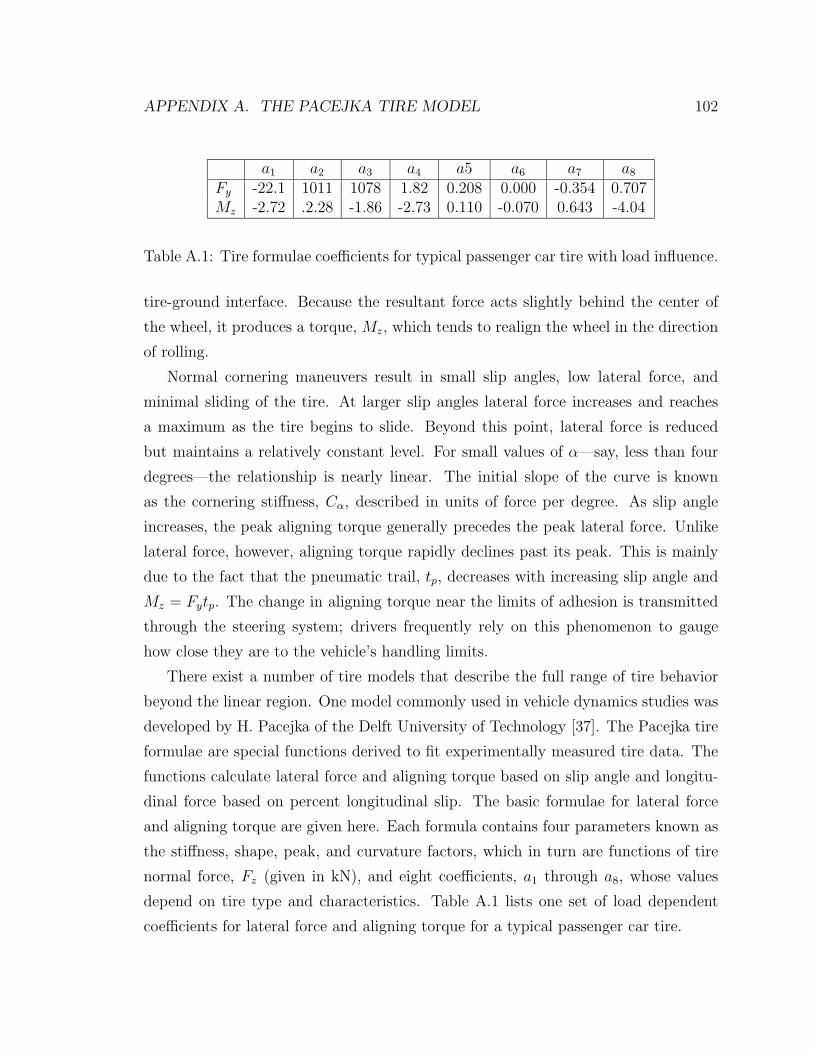
APPENDIX A. THE PACEJKA TIRE MODEL 102
a1 a2 a3 a4 a5 a6 a7 a8
Fy -22.1 1011 1078 1.82 0.208 0.000 -0.354 0.707Mz -2.72 .2.28 -1.86 -2.73 0.110 -0.070 0.643 -4.04
Table A.1: Tire formulae coefficients for typical passenger car tire with load influence.
tire-ground interface. Because the resultant force acts slightly behind the center of
the wheel, it produces a torque, Mz, which tends to realign the wheel in the direction
of rolling.
Normal cornering maneuvers result in small slip angles, low lateral force, and
minimal sliding of the tire. At larger slip angles lateral force increases and reaches
a maximum as the tire begins to slide. Beyond this point, lateral force is reduced
but maintains a relatively constant level. For small values of α—say, less than four
degrees—the relationship is nearly linear. The initial slope of the curve is known
as the cornering stiffness, Cα, described in units of force per degree. As slip angle
increases, the peak aligning torque generally precedes the peak lateral force. Unlike
lateral force, however, aligning torque rapidly declines past its peak. This is mainly
due to the fact that the pneumatic trail, tp, decreases with increasing slip angle and
Mz = Fytp. The change in aligning torque near the limits of adhesion is transmitted
through the steering system; drivers frequently rely on this phenomenon to gauge
how close they are to the vehicle’s handling limits.
There exist a number of tire models that describe the full range of tire behavior
beyond the linear region. One model commonly used in vehicle dynamics studies was
developed by H. Pacejka of the Delft University of Technology [37]. The Pacejka tire
formulae are special functions derived to fit experimentally measured tire data. The
functions calculate lateral force and aligning torque based on slip angle and longitu-
dinal force based on percent longitudinal slip. The basic formulae for lateral force
and aligning torque are given here. Each formula contains four parameters known as
the stiffness, shape, peak, and curvature factors, which in turn are functions of tire
normal force, Fz (given in kN), and eight coefficients, a1 through a8, whose values
depend on tire type and characteristics. Table A.1 lists one set of load dependent
coefficients for lateral force and aligning torque for a typical passenger car tire.
APPENDIX A. THE PACEJKA TIRE MODEL 103
A.1 Lateral force (Fy)
For the lateral force formula, the stiffness, shape, peak, and curvature factors—C, D,
B, and E, respectively—are calculated as follows.
C = 1.30 (A.1)
D = a1F2
z + a2Fz
B =a3 sin(a4 tan−1(a5Fz))
CDE = a6F
2
z + a7Fz + a8
The lateral force, Fy, for each tire is a function of these factors and the tire slip angle.
Fy = D sin(C tan−1(Bφ)) (A.2)
φ = (1 − E)α +E
Btan−1(Bα)
Note that to conform to the ISO standard sign conventions, the sign of the lateral
force calculated from this equation must be reversed when applied to the vehicle
model. Figure A.2 illustrates the tire lateral force as derived from Equation (A.3).
A.2 Aligning torque (Mz)
The factors for aligning torque are given by the following equations.
C = 2.40 (A.3)
D = a1F2
z + a2Fz
B =a3F
2z + a4Fz
ea5FzCDE = a6F
2
z + a7Fz + a8
Aligning torque, Mz, is a function of these factors and tire slip angle.
Mz = D sin(tan−1(Bφ)) (A.4)
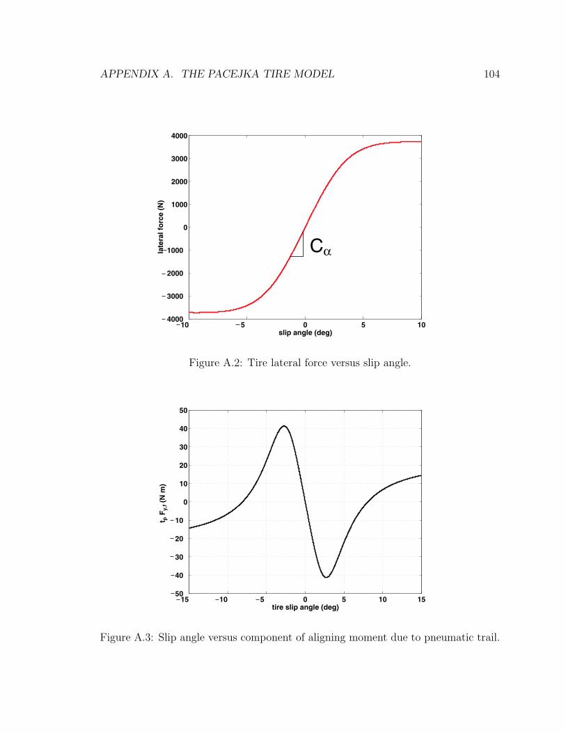
APPENDIX A. THE PACEJKA TIRE MODEL 104
10 5 0 5 104000
3000
2000
1000
0
1000
2000
3000
4000
slip angle (deg)
late
ral
forc
e (
N)
Cα
Figure A.2: Tire lateral force versus slip angle.
15 10 5 0 5 10 1550
40
30
20
10
0
10
20
30
40
50
tire slip angle (deg)
t p F
y,f (
N m
)
Figure A.3: Slip angle versus component of aligning moment due to pneumatic trail.
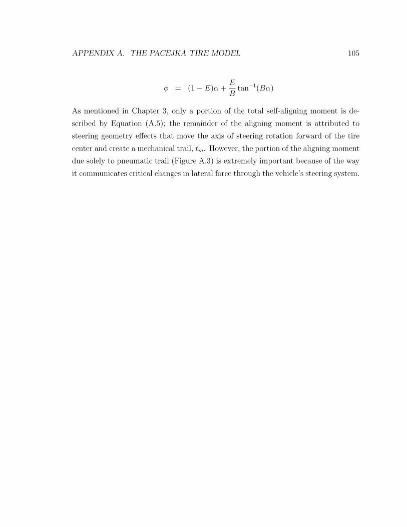
APPENDIX A. THE PACEJKA TIRE MODEL 105
φ = (1 − E)α +E
Btan−1(Bα)
As mentioned in Chapter 3, only a portion of the total self-aligning moment is de-
scribed by Equation (A.5); the remainder of the aligning moment is attributed to
steering geometry effects that move the axis of steering rotation forward of the tire
center and create a mechanical trail, tm. However, the portion of the aligning moment
due solely to pneumatic trail (Figure A.3) is extremely important because of the way
it communicates critical changes in lateral force through the vehicle’s steering system.
Appendix B
Hydraulic Power Assisted Steering
B.1 Power steering components
The key components of the hydraulic power assist system are the hydraulic pump, the
rotary spool valve, and the rack piston (Figure B.1). The rotary spool valve consists
of the torsion bar, inner spool, and outer sleeve. When the driver applies a torque
to the steering wheel, the torsion bar twists, and the inner spool rotates with respect
to the outer sleeve. This rotation of the valve opens metering orifices that increase
the flow of hydraulic fluid to one side of the rack piston while restricting flow to the
other side of the piston. The resulting differential pressure inside the cylinder pushes
the piston to one side or the other depending on the direction of steering. The piston
is connected to the steering rack, so hydraulic pressure directly translates to steering
effort.
B.2 Hydraulic model
Volumetric flow rate, Q, through an orifice is described by the following equation:
Q = ACd
√
2∆P
ρ(B.1)
106
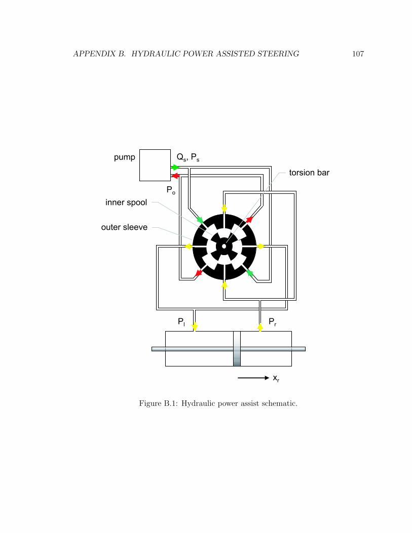
APPENDIX B. HYDRAULIC POWER ASSISTED STEERING 107
outer sleeve
inner spool
pump
torsion bar
xr
Pl Pr
Po
Qs, Ps
Figure B.1: Hydraulic power assist schematic.
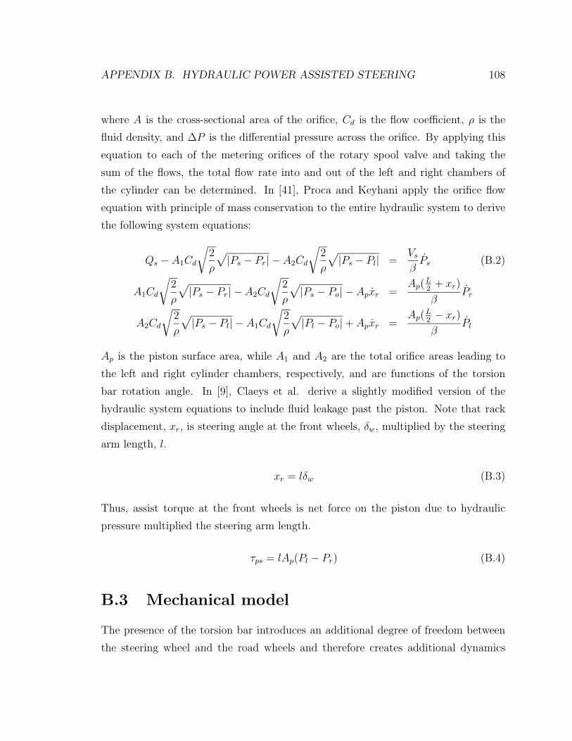
APPENDIX B. HYDRAULIC POWER ASSISTED STEERING 108
where A is the cross-sectional area of the orifice, Cd is the flow coefficient, ρ is the
fluid density, and ∆P is the differential pressure across the orifice. By applying this
equation to each of the metering orifices of the rotary spool valve and taking the
sum of the flows, the total flow rate into and out of the left and right chambers of
the cylinder can be determined. In [41], Proca and Keyhani apply the orifice flow
equation with principle of mass conservation to the entire hydraulic system to derive
the following system equations:
Qs − A1Cd
√
2
ρ
√
|Ps − Pr| − A2Cd
√
2
ρ
√
|Ps − Pl| =Vs
βPs (B.2)
A1Cd
√
2
ρ
√
|Ps − Pr| − A2Cd
√
2
ρ
√
|Ps − Po| − Apxr =Ap(
L2
+ xr)
βPr
A2Cd
√
2
ρ
√
|Ps − Pl| − A1Cd
√
2
ρ
√
|Pl − Po| + Apxr =Ap(
L2− xr)
βPl
Ap is the piston surface area, while A1 and A2 are the total orifice areas leading to
the left and right cylinder chambers, respectively, and are functions of the torsion
bar rotation angle. In [9], Claeys et al. derive a slightly modified version of the
hydraulic system equations to include fluid leakage past the piston. Note that rack
displacement, xr, is steering angle at the front wheels, δw, multiplied by the steering
arm length, l.
xr = lδw (B.3)
Thus, assist torque at the front wheels is net force on the piston due to hydraulic
pressure multiplied the steering arm length.
τps = lAp(Pl − Pr) (B.4)
B.3 Mechanical model
The presence of the torsion bar introduces an additional degree of freedom between
the steering wheel and the road wheels and therefore creates additional dynamics
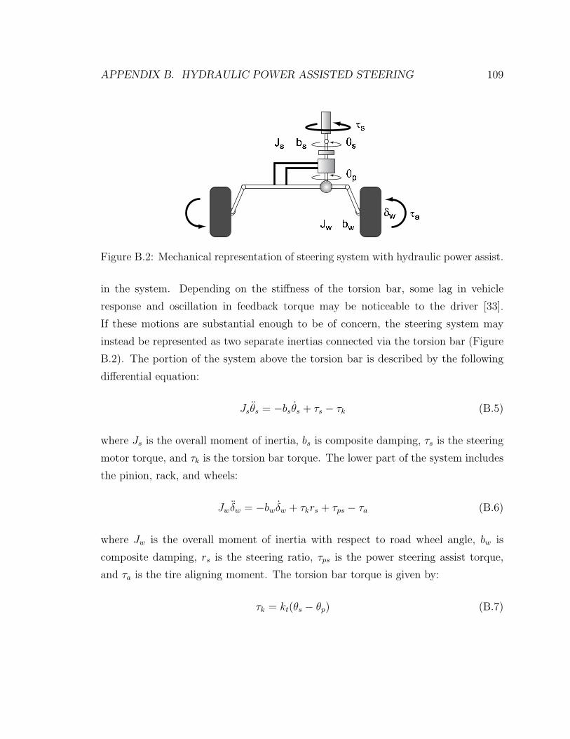
APPENDIX B. HYDRAULIC POWER ASSISTED STEERING 109
XY
Z[\[X[
]Z\
_[
_
Figure B.2: Mechanical representation of steering system with hydraulic power assist.
in the system. Depending on the stiffness of the torsion bar, some lag in vehicle
response and oscillation in feedback torque may be noticeable to the driver [33].
If these motions are substantial enough to be of concern, the steering system may
instead be represented as two separate inertias connected via the torsion bar (Figure
B.2). The portion of the system above the torsion bar is described by the following
differential equation:
Jsθs = −bsθs + τs − τk (B.5)
where Js is the overall moment of inertia, bs is composite damping, τs is the steering
motor torque, and τk is the torsion bar torque. The lower part of the system includes
the pinion, rack, and wheels:
Jwδw = −bwδw + τkrs + τps − τa (B.6)
where Jw is the overall moment of inertia with respect to road wheel angle, bw is
composite damping, rs is the steering ratio, τps is the power steering assist torque,
and τa is the tire aligning moment. The torsion bar torque is given by:
τk = kt(θs − θp) (B.7)
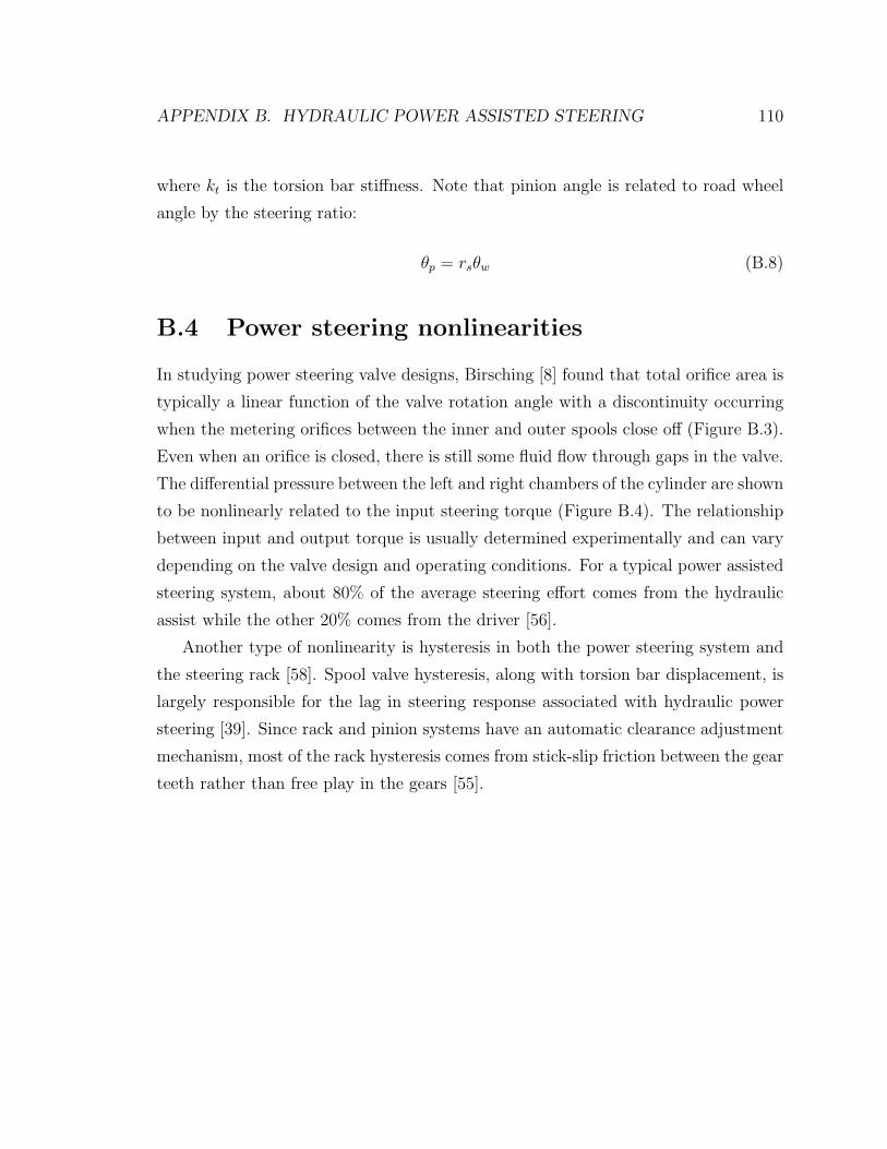
APPENDIX B. HYDRAULIC POWER ASSISTED STEERING 110
where kt is the torsion bar stiffness. Note that pinion angle is related to road wheel
angle by the steering ratio:
θp = rsθw (B.8)
B.4 Power steering nonlinearities
In studying power steering valve designs, Birsching [8] found that total orifice area is
typically a linear function of the valve rotation angle with a discontinuity occurring
when the metering orifices between the inner and outer spools close off (Figure B.3).
Even when an orifice is closed, there is still some fluid flow through gaps in the valve.
The differential pressure between the left and right chambers of the cylinder are shown
to be nonlinearly related to the input steering torque (Figure B.4). The relationship
between input and output torque is usually determined experimentally and can vary
depending on the valve design and operating conditions. For a typical power assisted
steering system, about 80% of the average steering effort comes from the hydraulic
assist while the other 20% comes from the driver [56].
Another type of nonlinearity is hysteresis in both the power steering system and
the steering rack [58]. Spool valve hysteresis, along with torsion bar displacement, is
largely responsible for the lag in steering response associated with hydraulic power
steering [39]. Since rack and pinion systems have an automatic clearance adjustment
mechanism, most of the rack hysteresis comes from stick-slip friction between the gear
teeth rather than free play in the gears [55].
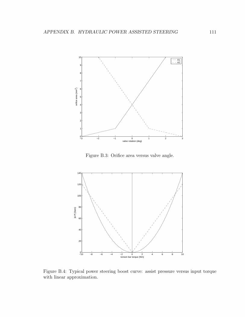
APPENDIX B. HYDRAULIC POWER ASSISTED STEERING 111
−3 −2 −1 0 1 2 30
1
2
3
4
5
6
7
8
9
10
valve rotation (deg)
orifi
ce a
rea
(mm
2 )
A1A2
Figure B.3: Orifice area versus valve angle.
−10 −8 −6 −4 −2 0 2 4 6 8 100
20
40
60
80
100
120
140
torsion bar torque (Nm)
|∆ P
| (ba
rs)
Figure B.4: Typical power steering boost curve: assist pressure versus input torquewith linear approximation.
Appendix C
Extension to Four-Wheel Steering
Vehicles
Four-wheel steering has often been proposed as a way to improve maneuverability,
stability, and controllability of all types of vehicles. It is a natural extension of the
modularity of the steer-by-wire concept.
C.1 Linear vehicle model with four-wheel steering
The bicycle model representation of a four-wheel steering vehicle (Figure C.1) adds
rear steering angle, δr. The state equations of motion for the bicycle model with front
and rear steering are given by:
[
βCG
r
]
=
[
−Cα,f−Cαr
mV−1 +
Cα,rb−Cα,fa
mV 2
Cα,rb−Cα,f a
Iz
−Cα,f a2−Cα,rb2
IzV
] [
βCG
r
]
+
[
Cα,f
mVCα,f a
Iz
]
δf +
[
Cα,r
mV
−Cα,rb
Iz
]
δr
(C.1)
112
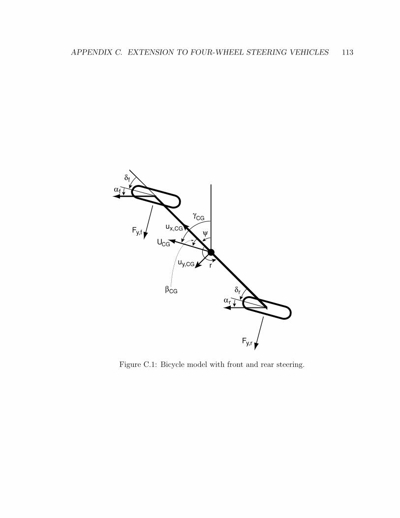
APPENDIX C. EXTENSION TO FOUR-WHEEL STEERING VEHICLES 113
αf
ruy,CG
ux,CGFy,f
βCG
γCG
ψ
UCG
αr
δr
δf
Fy,r
Figure C.1: Bicycle model with front and rear steering.
APPENDIX C. EXTENSION TO FOUR-WHEEL STEERING VEHICLES 114
C.2 Full state feedback vehicle control
A full state feedback control law for an active four-wheel steering vehicle is given by
δf = Kr,fr + Kβ,fβ + Kδ,fδf,d (C.2)
δr = Kr,rr + Kβ,rβ (C.3)
where δf,d is the driver commanded steer angle, δf is the augmented front steer angle,
and δr is the rear steer angle. Substituting the control law into Equation (C.1) yields:
[
βCG
r
]
=
[
−Cα,f−Cαr+Cα,f Kβ,f+Cα,rKβ,r
mV−1 +
Cα,rb−Cα,f a+Cα,f V Kr,f+Cα,rV Kr,r
mV 2
Cα,rb−Cα,f a+Cα,f aKβ,f−Cα,rbKβ,r
Iz
−Cα,f a2−Cα,rb2+Cα,f aV Kr,f−Cα,rbV Kr,r
IzV
] [
βCG
r
]
+
[
Cα,f Kδ,f
mVCα,f aKδ,f
Iz
]
δf,d (C.4)
Now, instead of targeting a new front cornering stiffness as in the active front steering
case, we aim to fractionally adjust the mass and moment of inertia of the four-wheel
steering vehicle:
Iz = Iz(1 + η) (C.5)
m = m(1 + η) (C.6)
This can be accomplished by choosing the state feedback gains as:
Kβ,f =η
1 + ηKr,f =
a
V
η
1 + ηKd,f =
1
1 + η(C.7)
Kβ,r = −η
1 + ηKr,r = −
b
V
η
1 + ηKd,r =
1
1 + η(C.8)
Substituting these feedback gains into the four-wheel steer model (Equation (C.4))
yields a state space model of the exact same form as the front wheel steer model
APPENDIX C. EXTENSION TO FOUR-WHEEL STEERING VEHICLES 115
(Equation (4.7)) but with the new mass, m, and moment of inertia, Iz:
[
βCG
r
]
=
[
−Cα,f−Cαr
mV−1 +
Cα,rb−Cα,fa
mV 2
Cα,rb−Cα,f a
Iz
−Cα,f a2−Cα,rb2
IzV
][
βCG
r
]
+
[
Cα,f
mVCα,f a
Iz
]
δ (C.9)
C.3 Limitations of four-wheel active steering
Again, suppose the desired vehicle handling characteristics are given by:
[
βCG
r
]
=
[
−Cα,f−Cαr
mV−1 +
Cα,r b−Cα,f a
mV 2
Cα,r b−Cα,f a
Iz
−Cα,f a2−Cα,r b2
IzV
][
βCG
r
]
+
[
Cα,f
mVCα,f a
Iz
]
δf,d (C.10)
Rewrite as[
βCG
r
]
=
[
a1,1 a1,2
a2,1 a2,2
][
βCG
r
]
+
[
b1
b2
]
δf,d (C.11)
and equate with Equation C.4:
−Cα,f − Cαr + Cα,fKβ,f + Cα,rKβ,r
mV= a1,1 (C.12)
−1 +Cα,rb − Cα,fa + Cα,fV Kr,f + Cα,rV Kr,r
mV 2= a1,2 (C.13)
Cα,rb − Cα,fa + Cα,faKβ,f − Cα,rbKβ,r
Iz
= a2,1 (C.14)
−Cα,fa2 − Cα,rb
2 + Cα,faV Kr,f − Cα,rbV Kr,r
IzV= a2,2 (C.15)
Cα,fKδ,f
mV= b1 (C.16)
Cα,faKδ,f
Iz
= b2 (C.17)
In contrast to the front-wheel steering case, the full state feedback gains, Kβ,f , Kβ,r,
Kr,f , and Kr,r, can be expressed explicitly in terms of the desired vehicle parameters,
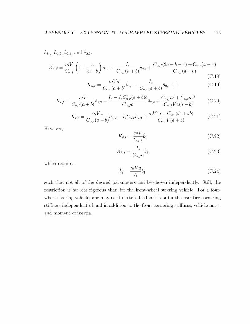
APPENDIX C. EXTENSION TO FOUR-WHEEL STEERING VEHICLES 116
a1,1, a1,2, a2,1, and a2,2:
Kβ,f =mV
Cα,f
(
1 +a
a + b
)
a1,1 +Iz
Cα,f (a + b)a2,1 +
Cα,f (2a + b − 1) + Cα,r(a − 1)
Cα,f (a + b)(C.18)
Kβ,r =mV a
Cα,r(a + b)a1,1 −
Iz
Cα,r(a + b)a2,1 + 1 (C.19)
Kr,f =mV
Cα,f (a + b)a1,2 +
Iz − IzC2α,r(a + b)b
Cα,faa2,2 +
Cα,fa3 + Cα,rab2
Cα,fV a(a + b)(C.20)
Kr,r =mV a
Cα,r(a + b)a1,2 − IzCα,ra2,2 +
mV 2a + Cα,r(b2 + ab)
Cα,rV (a + b)(C.21)
However,
Kδ,f =mV
Cα,f
b1 (C.22)
Kδ,f =Iz
Cα,fab2 (C.23)
which requires
b2 =mV a
Iz
b1 (C.24)
such that not all of the desired parameters can be chosen independently. Still, the
restriction is far less rigorous than for the front-wheel steering vehicle. For a four-
wheel steering vehicle, one may use full state feedback to alter the rear tire cornering
stiffness independent of and in addition to the front cornering stiffness, vehicle mass,
and moment of inertia.
Bibliography
[1] M. Abe, Y. Kano, K. Suzuki, Y. Shibahata, and Y. Furukawa. An experimental
validation of side-slip control to compensate vehicle lateral dynamics for a loss of
stability due to nonlinear tire characteristics. In Proceedings of the International
Symposium on Advanced Vehicle Control (AVEC), Ann Arbor, MI, pages 36–41,
2000.
[2] T. Acarman, K. A. Redmill, and U. Ozguner. A robust controller design for drive
by wire hydraulic power steering system. In Proceedings of the 2002 American
Control Conference, Anchorage, AK, pages 2522–2527, 2002.
[3] J. Ackermann. Yaw disturbance attenuation by robust decoupling of car steering.
In Proceedings of the IFAC World Congress, San Francisco, CA, pages 1–6, 1996.
[4] M. Aga and A. Okada. Analysis of vehicle stability control (VSC)’s effectiveness
from accident data. In Proceedings of the 18th International Technical Conference
on the Enhanced Safety of Vehicles, Nagoya, Japan, 2003.
[5] S. Amberkar, M. Kushion, K. Eschtruth, and F. Bolourchi. Diagnostic develop-
ment for an electric power steering system. SAE Technical Paper Series 2000-
01-0819, 2000.
[6] A. Badawy, J. Zuraski, F. Bolourchi, and A. Chandy. Modeling and analysis of
an electric power steering system. SAE Technical Paper Series 1999-01-0399,
1999.
[7] E. J. Bedner and H. H. Chen. A supervisory control to manage brakes and
four-wheel-steer systems. SAE Technical Paper Series 2004-01-1059, 2004.
117
BIBLIOGRAPHY 118
[8] J. E. Birsching. Two dimesional modeling ofa rotary power steering valve. SAE
Technical Paper Series 1999-01-0396, 1999.
[9] X. Claeys, C. Canudas de Wit, and H. Bechart. Modeling and control of steering
actuator for heavy duty vehicles. In Proceedings of the 1999 European Control
Conference, Karlsruhe, Germany, 1999.
[10] J. N. Dang. Preliminary results analyzing the effectiveness of electronic stability
(ESC) systems. NHTSA Evaluation Note DOT HS 809 790, 2004.
[11] J. C. Dixon. Tires, Suspension and Handling. Society of Automotive Engineers,
Warrendale, PA, 1996.
[12] C. M. Farmer. Effecto of electronic stability control on automobile crash risk.
Traffic Injury Prevention, 5:317–325, 2004.
[13] Y. Fukada. Slip-angle estimation for vehicle stability control. Vehicle System
Dynamics, 32:375–388, 2000.
[14] C. D. Gadda, P. Yih, and J. C. Gerdes. Incorporating a model of vehicle dy-
namics in a diagnostic system for steer-by-wire vehicles. In Proceedings of the
International Symposium on Advanced Vehicle Control (AVEC), Arnheim, The
Netherlands, pages 779–784, 2004.
[15] J. C. Gerdes and E. Rossetter. A unified approach to driver assistance systems
based on artifical potential fields. ASME Journal of Dynamic Systems, Measure-
ment, and Control, 123:431–438, 2001.
[16] M. Hiemer, U. Kiencke, T. Matsunaga, and K. Shirasawa. Cornering stiffness
adaptation for improved side slip angle observation. In Proceedings of the IFAC
Symposium on Advances in Automotive Control, Salerno, Italy, pages 685–690,
2004.
[17] A. Higuchi and Y. Saito. Optimal control of four wheel steering vehicle. In Pro-
ceedings of the International Symposium on Advanced Vehicle Control (AVEC),
Yokohama, Japan, pages 233–238, 1992.
BIBLIOGRAPHY 119
[18] S. Horiuchi and N. Yuhara. An analytical approach to the prediction of handling
qualities of vehicles with advanced steering control system using multi-input
driver model. ASME Journal of Dynamic Systems, Measurement, and Control,
122:490–497, 2000.
[19] Y. J. Hsu and J. C. Gerdes. Stabilization of a steer-by-wire vehicle at the limits of
handling using feedback linearization. Submitted to the 2005 American Control
Conference, Portland, OR, 2005.
[20] K. Huh and J. Kim. Active steering control based on the estimated tire forces.
ASME Journal of Dynamic Systems, Measurement, and Control, 123:505–511,
2001.
[21] H. Inagaki, K. Akuzawa, and M. Sato. Yaw rate feedback braking force distri-
bution control with control-by-wire braking system. In Proceedings of the Inter-
national Symposium on Advanced Vehicle Control (AVEC), Yokohama, Japan,
1992.
[22] Y. Jeong, D. Kim, K. Kim, D. Hwang, K. Oh, and T. Koh. Development of a
steering sensor for vehicle control systems. In Proceedings of the International
Symposium on Advanced Vehicle Control (AVEC), Nagoya, Japan, pages 213–
217, 1998.
[23] J. Kasselmann and T. Keranen. Adaptive steering. Bendix Technical Journal,
2:26–35, 1969.
[24] W. M. Kauffman, C. J. Liddell, A. Smith, and R. D. VanDyke. An apparatus
for varying effective dihedral in flight with application to a study of tolerable
dihedral on a conventional fighter airplane. National Advisory Committee for
Aeronautics Report 948, 1949.
[25] K. Langwieder, J. Gwehenberger, T. Hummel, and J. Bende. Benefit potential
of ESP in real accident situations involving cars and trucks. In Proceedings of
the 18th International Technical Conference on the Enhanced Safety of Vehicles,
Nagoya, Japan, 2003.
BIBLIOGRAPHY 120
[26] S. Laws, S. Kohn, C. D. Gadda, P. Yih, J. C. Gerdes, and J. C. Milroy. Steer-
by-wire suspension design for controllability. Submitted to the 16th IFAC World
Congress, Prague, Czech Republic, 2005.
[27] A. Y. Lee. Matching vehicle responses using the model-following control method.
SAE Technical Paper Series 970561, 1997.
[28] A. Lie, C. Tingvall, M. Krafft, and A. Kullgren. The effectiveness of ESP (elec-
tronic stability program) in reducing real life accidents. Traffic Injury Prevention,
5:37–41, 2004.
[29] A. Liu and S. Chang. Force feedback in a stationary driving simulator. In Proceed-
ings of the IEEE International Conference on Systems, Man, and Cybernetics,
volume 2, pages 1711–1716, 1995.
[30] H. Lupker, J. Zuurbier, R. Verschuren, S. Jansen, and D. Willemsen. Steer-by-
wire innovations and demonstrator. In Proceedings of the International Sympo-
sium on Advanced Vehicle Control (AVEC), Hiroshima, Japan, pages 665–670,
2002.
[31] S. Mammar and D. Koenig. Vehicle handling improvement by active steering.
Vehicle System Dynamics, 38:211–242, 2002.
[32] R. McCann. Variable effort steering for vehicle stability enhancement using an
electric power steering system. SAE Technical Paper Series 2000-01-0817, 2000.
[33] V. D. Mills and J. R. Wagner. Behavioural modelling and analysis of hybrid
vehicle steering systems. IMechE Journal of Automobile Engineering, 217:349–
361, 2003.
[34] M. Nagai, S. Yamanaka, and Y. Hirano. Integrated control law of active rear
wheel steering and direct yaw moment control. In Proceedings of the International
Symposium on Advanced Vehicle Control (AVEC), Aachen, Germany, pages 451–
470, 1996.
BIBLIOGRAPHY 121
[35] E. Ono, S. Hosoe, H. D. Tuan, and S. Doi. Bifurcation in vehicle dynamics
and robust front wheel steering control. IEEE Transactions on Control Systems
Technology, 6:412–420, 1998.
[36] A. Y. Orbak, K. Youcef-Toumi, and M. Senga. Model reduction and design of a
power steering system. In Proceedings of the 1999 American Control Conference,
San Diego, CA, pages 4476–4481, 1999.
[37] H. Pacejka, E. Bakker, and L. Nyborg. Tyre modelling for use in vehicle dynamic
studies. SAE Technical Paper Series 870421, 1987.
[38] Y. E. Papelis, T. Brown, G. Watson, D. Holtz, and W. Pan. Study of ESC
assisted driver performance using a driving simulator. National Advanced Driving
Simulator Document ID N04-003-PR, 2004.
[39] J. P. Pauwelussen and J. J. A. Pauwelussen. Exploration of steering wheel angle
based workload measures in relationship to steering feel evaluation. In Pro-
ceedings of the International Symposium on Advanced Vehicle Control (AVEC),
Arnheim, The Netherlands, pages 427–432, 2004.
[40] D. Peter and R. Gerhard. Electric power steering—the first step on the way to
steer by wire. SAE Technical Paper Series 1999-01-0401, 1999.
[41] A. B. Proca and A. Keyhani. Identification of power steering dynamic models.
Mechatronics, 8:255–270, 1998.
[42] H. S. Radt. Variable Dynamic Testbed Vehicle: Analysis of Handling Per-
formance With and Without Rear Steer. Milliken Research Associates, Inc.,
Williamsville, NY, 1997.
[43] E. J. Rossetter. A Potential Field Framework for Active Vehicle Lanekeeping
Assistance. PhD thesis, Stanford University, December 2003.
[44] J. Ryu and J. C. Gerdes. Integrating inertial sensors with global positioning
system (GPS) for vehicle dynamics control. ASME Journal of Dynamic Systems,
Measurement, and Control, 126:243–254, 2004.
BIBLIOGRAPHY 122
[45] J. Ryu, E. Rossetter, and J. C. Gerdes. Vehicle sideslip and roll parameter esti-
mation using GPS. In Proceedings of the International Symposium on Advanced
Vehicle Control (AVEC), Hiroshima, Japan, pages 373–380, 2002.
[46] C. L. Seacord and D. K. Vaughn. Preliminary system design for a digital fly-
by-wire flight control system for an F-8C aircraft. NASA Center for Aerospace
Information NASA-CR-2609, 1976.
[47] R. Sebastian, T. Kaufmann, F. Bolourchi, and H. S. Tan. Design of an automated
highway systems steering actuator control system. In Proceedings of the IEEE
Conference on Intelligent Transportation Systems, pages 254–259, 1997.
[48] M. Segawa, K. Nishizaki, and S. Nakano. A study of vehicle stability control by
steer by wire system. In Proceedings of the International Symposium on Advanced
Vehicle Control (AVEC), Ann Arbor, MI, pages 7–12, 2000.
[49] R. S. Sharp and R. Granger. On car steering torques at parking speeds. IMechE
Journal of Automobile Engineering, 217:87–96, 2003.
[50] R. Subramanian. Analysis of crashes involving 15-passenger vans. NHTSA Tech-
nical Report DOT HS 809 735, 2004.
[51] J. P. Switkes, E. J. Rossetter, I. A. Coe, and J. C. Gerdes. Handwheel force
feedback for lanekeeping assistance: Combined dynamics and stability. In Pro-
ceedings of the International Symposium on Advanced Vehicle Control (AVEC),
Arnheim, The Netherlands, pages 47–52, 2004.
[52] J. Tajima and N. Yuhara. Effects of steering system characteristics on control
performance from the viewpoint of steer-by-wire system design. SAE Technical
Paper Series 1999-01-0821, 1999.
[53] A. Taneda and T. Yamanaka. Design of actuator for active-rear-steer system.
SAE Technical Paper Series 981114, 1998.
BIBLIOGRAPHY 123
[54] A. van Zanten. Evolution of electronic control systems for improving the vehicle
dynamic behavior. In Proceedings of the International Symposium on Advanced
Vehicle Control (AVEC), Hiroshima, Japan, pages 7–15, 2002.
[55] A. Wohnhaas and U. Essers. Nonlinear modeling and simulation of a rack and
pinion steering. In Proceedings of the International Symposium on Advanced
Vehicle Control (AVEC), Yokohama, Japan, pages 68–73, 1992.
[56] T. Wong. Hydraulic power steering system design and optimization simulation.
SAE Technical Paper Series 2000-01-0479, 2001.
[57] Y. Yasui, W. Tanaka, E. Ono, Y. Muragishi, K. Asano, M. Momiyama, S. Ogawa,
K. Asano, Y. Imoto, and H. Kato. Wheel grip factor estimation apparatus. United
States Patent Application Pub. No. US 2004/0019417 A1, 2004.
[58] J. Yu, J. Aston, C. Gilsinger, J. Shutway, and H. Tokunaga. Vehicle dynamic
feeling study with a focus on the on-center steering feeling of north ameridcan
highway driving. In Proceedings of the International Symposium on Advanced
Vehicle Control (AVEC), Arnheim, The Netherlands, pages 415–420, 2004.
[59] N. Yuhara and J. Tajima. Advanced steering system adaptable to lateral control
task and driver’s intention. Vehicle System Dynamics, 36:119–158, 2000.
[60] N. Yuhara, J. Tajima, S. Sano, and S. Takimoto. Steer-by-wire-oriented steering
system design: Concept and examination. Vehicle System Dynamics, 33:692–703,
2000.


![Vehicle Handling Improvement with Steer-by-Wire System ... · of vehicle handling and stability using SBW architecture. Yih [4] addressed some of the issues associated with control](https://img.pdfslide.us/doc/110x75/603d5ce6e7773477283d0a48/vehicle-handling-improvement-with-steer-by-wire-system-of-vehicle-handling-and.jpg)