metals

Article

Sensitivity Analysis in the Modelling of a High SpeedSteel Thin-Wall Produced by DirectedEnergy Deposition

Rúben Tome Jardin 1, Víctor Tuninetti 2,* , Jérôme Tchoufang Tchuindjang 3 , Neda Hashemi 3,Raoul Carrus 4, Anne Mertens 3 , Laurent Duchêne 1, Hoang Son Tran 1 andAnne Marie Habraken 1,5,*

1 Department ArGEnCo-MSM, University of Liège, Quartier Polytech 1, allée de la Découverte 9,4000 Liège, Belgium; ra.tjardin@ulg.ac.be (R.T.J.); l.duchene@uliege.be (L.D.); hstran@uliege.be (H.S.T.)

2 Department of Mechanical Engineering, Universidad de La Frontera, Francisco Salazar 01145,Temuco 4780000, Chile

3 Department A&M–MMS, University of Liège, Quartier Polytech 1, allée de la Découverte 9,4000 Liège, Belgium; j.tchuindjang@uliege.be (J.T.T.); s.neda.hashemi@gmail.com (N.H.);anne.mertens@uliege.be (A.M.)

4 Sirris Research Centre (Liège), Rue Bois St-Jean 12, 4102 Seraing, Belgium; raoul.Carrus@sirris.be5 Fonds de la Recherche Scientifique–F.R.S.-F.N.R.S., 1000 Brussels, Belgium* Correspondence: victor.tuninetti@ufrontera.cl (V.T.); anne.habraken@uliege.be (A.M.H.);

Tel.: +56-452325984 (V.T.); +32-496607945 (A.M.H.)

Received: 29 October 2020; Accepted: 19 November 2020; Published: 22 November 2020 �����������������

Abstract: This paper reports the sensitivity of the thermal and the displacement histories predictedby a finite element analysis to material properties and boundary conditions of a directed-energydeposition of a M4 high speed steel thin-wall part additively manufactured on a 42CrMo4 steelsubstrate. The model accuracy was assessed by comparing the simulation results with the experimentalmeasurements such as evolving local temperatures and distortion of the substrate. The numericalresults of thermal history were successfully correlated with the solidified microstructures measured byscanning electron microscope technique, explaining the non-uniform, cellular-type grains dependingon the deposit layers. Laser power, thermal conductivity, and thermal capacity of deposit andsubstrate were considered in the sensitivity analysis in order to quantify the effect of their variationson the local thermal history, while Young’s modulus and yield stress variation effects were evaluatedon the distortion response of the sample. The laser power showed the highest impact on the thermalhistory, then came the thermal capacity, then the conductivity. Considering distortion, variations ofthe Young’s modulus had a higher impact than the yield stress.

Keywords: DED additive process; thin-wall deposit experiment; distortion; thermal history;finite element simulation; thermomechanical model; M4 steel

1. Introduction

Within the additive manufacturing (AM) processes, directed-energy deposition (DED) is a genericname for layered manufacturing of fully dense parts based on progressive welding of a wire or metalpowder (Figure 1) on a substrate. The energy sources required for melting the feed metal in DEDprocesses can be provided by electron beam (EB), laser (L), plasma, or electric arc. The most knownDED processes are laser cladding (LC) or laser metal deposition (LMD) such as wire-based laser metaldeposition (LMD-W) or powder-based laser metal deposition (LMD-P), electron beam melting (EBM)

Metals 2020, 10, 1554; doi:10.3390/met10111554 www.mdpi.com/journal/metals

Metals 2020, 10, 1554 2 of 25

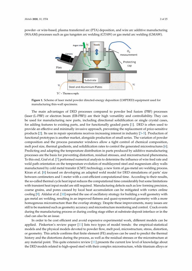
powder- or wire-based, plasma transferred arc (PTA) deposition, and wire arc additive manufacturing(WAAM) processes such as gas tungsten arc welding (GTAW) or gas metal arc welding (GMAW).

Metals 2020, 10, x FOR PEER REVIEW 2 of 24

melting (EBM) powder- or wire-based, plasma transferred arc (PTA) deposition, and wire arc additive manufacturing (WAAM) processes such as gas tungsten arc welding (GTAW) or gas metal arc welding (GMAW).

Figure 1. Scheme of laser metal powder directed-energy deposition (LMPDED) equipment used for manufacturing thin-wall specimens.

The main advantages of DED processes compared to powder bed fusion (PBF) processes (laser (L-PBF) or electron beam (EB-PBF)) are their high versatility and controllability. They can be used for manufacturing new parts, including directional solidification or single crystal cases, for adding features to existing parts, and for functionally graded parts [1]. DED is often used to provide an effective and minimally invasive approach, preventing the replacement of price-sensitive products [2]. Its use in repair operations receives increasing interest in industry [3–5]. Production of functional prototypes is another market, alongside production of small series. The variation of powder composition and the process parameter windows allow a tight control of chemical composition, melt pool size, thermal gradients, and solidification rates to control the generated microstructures [6]. Predicting and adapting the temperature distribution in parts produced by additive manufacturing processes are the basis for preventing distortion, residual stresses, and microstructural phenomena. To this end, Graf et al. [7] performed numerical analysis to determine the influence of wire feed rate and weld path orientation on the temperature evolution of multilayered steel and magnesium alloy walls manufactured by cold metal transfer (CMT) technology, a new form of gas-metal arc-welding process. Kiran et al. [8] focused on developing an adapted weld model for DED simulations of parts’ size between centimeters and 1 meter with a cost-efficient computational time. According to their results, the so-called thermal cycle heat input reduces the computational time considerably but some limitations with transient heat input model are still required. Manufacturing defects such as low forming precision, coarse grains, and pores caused by local heat accumulation can be mitigated with vortex online cooling [9]. Aldalur et al. [10] reported the use of oscillatory strategy for building a wall geometry with gas metal arc welding, resulting in an improved flatness and quasi-symmetrical geometry with a more homogenous microstructure than the overlap strategy. Despite these improvements, many issues are still to be mastered such as geometry accuracy and microstructure monitoring and control. Crack events during the manufacturing process or during cooling stage either at substrate-deposit interface or in the clad can also be an issue.

In order to be cost efficient and avoid expensive experimental work, different models can be applied. Pinkerton’s review paper [11] lists two types of model trends: the empirical-statistical models and the physical models devoted to powder flow, melt pool, microstructure, stress, distortion, or geometry. This article confirms that finite element (FE) analyses can be used to predict the thermal history and the distortions during the process, as well as the residual stresses or the microstructure at any material point. This quite extensive review [11] presents the current low level of knowledge about the DED models related to high-speed steel with their complex microstructure, while titanium

Figure 1. Scheme of laser metal powder directed-energy deposition (LMPDED) equipment used formanufacturing thin-wall specimens.

The main advantages of DED processes compared to powder bed fusion (PBF) processes(laser (L-PBF) or electron beam (EB-PBF)) are their high versatility and controllability. They canbe used for manufacturing new parts, including directional solidification or single crystal cases,for adding features to existing parts, and for functionally graded parts [1]. DED is often used toprovide an effective and minimally invasive approach, preventing the replacement of price-sensitiveproducts [2]. Its use in repair operations receives increasing interest in industry [3–5]. Production offunctional prototypes is another market, alongside production of small series. The variation of powdercomposition and the process parameter windows allow a tight control of chemical composition,melt pool size, thermal gradients, and solidification rates to control the generated microstructures [6].Predicting and adapting the temperature distribution in parts produced by additive manufacturingprocesses are the basis for preventing distortion, residual stresses, and microstructural phenomena.To this end, Graf et al. [7] performed numerical analysis to determine the influence of wire feed rate andweld path orientation on the temperature evolution of multilayered steel and magnesium alloy wallsmanufactured by cold metal transfer (CMT) technology, a new form of gas-metal arc-welding process.Kiran et al. [8] focused on developing an adapted weld model for DED simulations of parts’ sizebetween centimeters and 1 meter with a cost-efficient computational time. According to their results,the so-called thermal cycle heat input reduces the computational time considerably but some limitationswith transient heat input model are still required. Manufacturing defects such as low forming precision,coarse grains, and pores caused by local heat accumulation can be mitigated with vortex onlinecooling [9]. Aldalur et al. [10] reported the use of oscillatory strategy for building a wall geometry withgas metal arc welding, resulting in an improved flatness and quasi-symmetrical geometry with a morehomogenous microstructure than the overlap strategy. Despite these improvements, many issues arestill to be mastered such as geometry accuracy and microstructure monitoring and control. Crack eventsduring the manufacturing process or during cooling stage either at substrate-deposit interface or in theclad can also be an issue.

In order to be cost efficient and avoid expensive experimental work, different models can beapplied. Pinkerton’s review paper [11] lists two types of model trends: the empirical-statisticalmodels and the physical models devoted to powder flow, melt pool, microstructure, stress, distortion,or geometry. This article confirms that finite element (FE) analyses can be used to predict the thermalhistory and the distortions during the process, as well as the residual stresses or the microstructure atany material point. This quite extensive review [11] presents the current low level of knowledge aboutthe DED models related to high-speed steel with their complex microstructure, while titanium alloys or

Metals 2020, 10, 1554 3 of 25

superalloys have been extensively studied. It reminds also that non-equilibrium material state presentin DED process prevents easy use of classical continuous cooling transformation diagrams.

The simulation targets usually define the model scale. For instance, to prevent balling effect andunderstand pore formation, detailed melt pool modeling and fluid simulations cannot be avoided.Note that with such a fluid methodology, in DED, Khairallah et al. [12] explains the flaw mechanismfor both stainless steel 316L and nickel-based superalloy IN738LC, while Heeling et al. [13] presentsthe optimization of the process parameters for stainless steel. However, the micro scale of thesemodels prevents them from addressing the simulations of whole parts, while even lower scale andother types of models, for instance, phase field approach [14,15], would be required to analyze thesegregation behavior and the generation of phases. As explained by Jardin et al. [16], the precipitationof the carbides within M4 cladding results in a heterogeneous distribution of the carbide shape, size,and nature along the depth of a cladded sample. A phase field model is a further step for University ofLiège team. Another example of the interest of low-scale method is the study of the diffusion betweenSi inclusions and Al matrix for AlSi10Mg determining the rupture location [17].

At the macroscopic scale, more adapted to industrial parts, the inherent strain-based method [18]is often used. It assumes incompatible strains from different sources and decouples stress components.However, the accuracy of this method for complex parts is not guaranteed and a careful calibrationis always required either based on direct experiments or based on a detailed validated simulation.Detailed FE simulations close to the physical phenomena is this paper’s scope. It provides a deeperunderstanding of the material history within the process and helps to identify its control parameters.However, those simulations still present computer’s central processing unit (CPU) issues, which limitthem to simple parts. As demonstrated hereafter, the mechanical result accuracy is not guaranteed forcomplex material as M4 steel deposited on 42CrMo4 substrate.

As the thermal field is the key factor, numerous 2D and 3D FE simulations at the macroscopic scalehave been developed for academic samples providing the thermal history of deposits. For instance,special focus on the heat-affected zone is chosen by Yang et al. [19], while the effect of thelaser scanning speed on the thermal evolution and on the melt pool size is studied by Patil andYadava [20], of laser power by Yin et al. [21], and of preheating temperature by Chiumenti et al. [22].However, those previous works do not discuss the impact of the accuracy of the input materialparameter data on their predictions. Often by lack of knowledge, strong simplifications are done.A common simple assumption is to neglect the variations of the thermophysical properties with thetemperature [23] or adopting constant heat convection coefficient for the boundary conditions [24],while the variation of this coefficient with the geometry and the temperature was demonstrated by [25].The shape of the heat input developed by Goldak’s work [26], intended to model the laser beam heatsource, could be used. However, a constant local value of heat input or a simplified shape is oftenadopted [27,28].

Another cutoff from the complex physics concerns the geometry of the added material at eachtrack within a new layer of added material. By convenience, it is often a cuboid volume related tomean size of the track height and the track width. Within thermomechanical solid FE simulations,only some models like the one of Lindgren et al. [29] compute the added volume shape based onphysical assumptions. Another way was chosen by Caiazzo et al. [30], who define it by regressionformulas based on an extensive experimental campaign.

Key material information such as visco-plastic behavior within the mechanical model isusually based on experimental measurements from samples not manufactured by DED [29].However, as pointed out by Lu and his coworkers [31], this approach is not reliable to generateaccurate predictions as mechanical and thermophysical properties strongly depend on microstructuresthat are different in casting, forging, or additive manufacturing processes. The sensitivity analysis ofLu et al. [31] about the effect of mechanical properties of Ti-6Al-4V alloy shows that the distortion andresidual stresses strongly depend on the values of the thermal expansion coefficient and the elasticlimit, while slightly on the Young’s modulus.

Metals 2020, 10, 1554 4 of 25

The present research focused on a thin-wall sample of 10 layers of M4 material on a substrate in42CrMo4 steel. Thermomechanical finite element simulations compute thermal history of the claddedmaterial as well as distortion and local temperature of substrate. As shown next, the access to accuratematerial data for this specific high-speed steel (HSS) grade is more problematic than CPU issues.A thorough validation of the model results was conducted using the predicted displacement andtemperature curves of different points in the material, which were compared with their correspondingmeasured values throughout the process, including substrate preheating, deposition, and cooling.Final microstructure was measured by optical and scanning electron microscopy performed at themiddle cross-section of the thin wall and substrate for further correlation analysis with the thermalhistory. Note that M4 material was selected because of its enhanced performances in wear and hardnesswhen manufactured by DED [32,33]. However high amount of carbon in the material compositioncombined with thermal and/or phase-transformation stresses generates a high susceptibility to crackformation [34,35]. This feature explains why DED of tool steels remains very challenging. In additionto the usual process parameters, such as laser power, scanning speed, powder flow rate, and scanningstrategy (laser path, idle time, track interdistance), the identification of the preheating temperaturelevel is a mandatory step.

The cracks easily appear due to the tensile stress generated in the clad bottom or at theclad–substrate interface during the cladding process. The preheating temperature of the substratedecreases the space thermal gradient and the cooling rate and minimizes the thermal distortionsand stresses during the process. As shown by Leunda et al. [36] for CPM 10V and Vanadis 4 extratool steel powders, the crack appearances can be avoided by a preheating temperature below themaximum tempering temperature. For M4 powder, Shim et al. [32] specifically analyzed the effectsof the substrate preheating on the metallurgical and mechanical characteristics of the manufacturedparts. The results enhanced the effect of the preheating on the cooling history and solidification rates.Specimens without preheating mainly include equiaxial fine grains, whereas the induction-heatedspecimens generate columnar grains. However, no significant hardness differences were measured,which could be explained by secondary hardening mechanism caused by hard and stable carbides.As pointed by Jardin et al. [16], for a preheating of 300 ◦C and a 36-layer clad of 40 × 40 × 27.5 mm3

(a bulk sample compared to the thin-wall geometry studied here) a strong heterogeneity appears withinthe clad deposit due to different thermal histories. Close to the deposit-free surface and at mid-height,the angular-like vanadium-rich metal carbides (MC) carbides precipitated in intercellular zones justafter the primary cells. The high superheating temperature within the melt pool at mid-height of thedeposit promotes the coarsening of the solidification phases including cells and intercellular carbides.At intermediate depth of 4.5 mm from the deposit-free surface, a lower superheating temperature and ahigher number of remelting of the material points promote the precipitation of coral-like vanadium-richMC carbides inside cells.

The present article aimed to quantify the variation of the numerical predictions due to differentmaterial properties such as stress–strain relationship, thermophysical variables, or boundary conditionssuch as convection and radiation flow. The prediction of distortion currently achieved lacks precisionwhen compared with experimental results. However, forthcoming work on improving predictions,reducing residual stress, and increasing microstructure homogeneity will be based on numericaloptimization. The complexity of the multiphase materials of both the clad and the substrate demonstratesthat the model sensitivity analysis presented in this work is a required stage for obtaining reliable results.

The paper describes the thin-wall experiment in Section 2.1, the metallographic observationsin Section 2.2, and the FE model in Section 2.3. The results of the material data measurementsare provided in Sections 3.1 and 3.2. The validation of the model was performed through acomparison between thermal history predictions of the substrate with experimental results in Section 4.1.In Section 4.2, the observed microstructure by optical microscopy (OM) and scanning electronmicroscopy (EM) is explained based on the predicted thermal history of the clad. The thermal and

Metals 2020, 10, 1554 5 of 25

thermomechanical sensitivity analyses and discussions are given in Sections 4.3 and 4.4, respectively.Finally, Section 5 provides the summary of the key results and the perspectives for ongoing research.

2. Materials and Methods

2.1. Thin-Wall Experiments

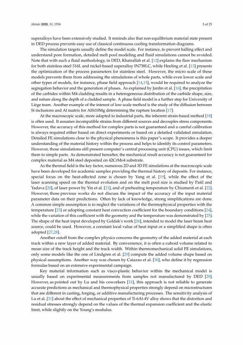
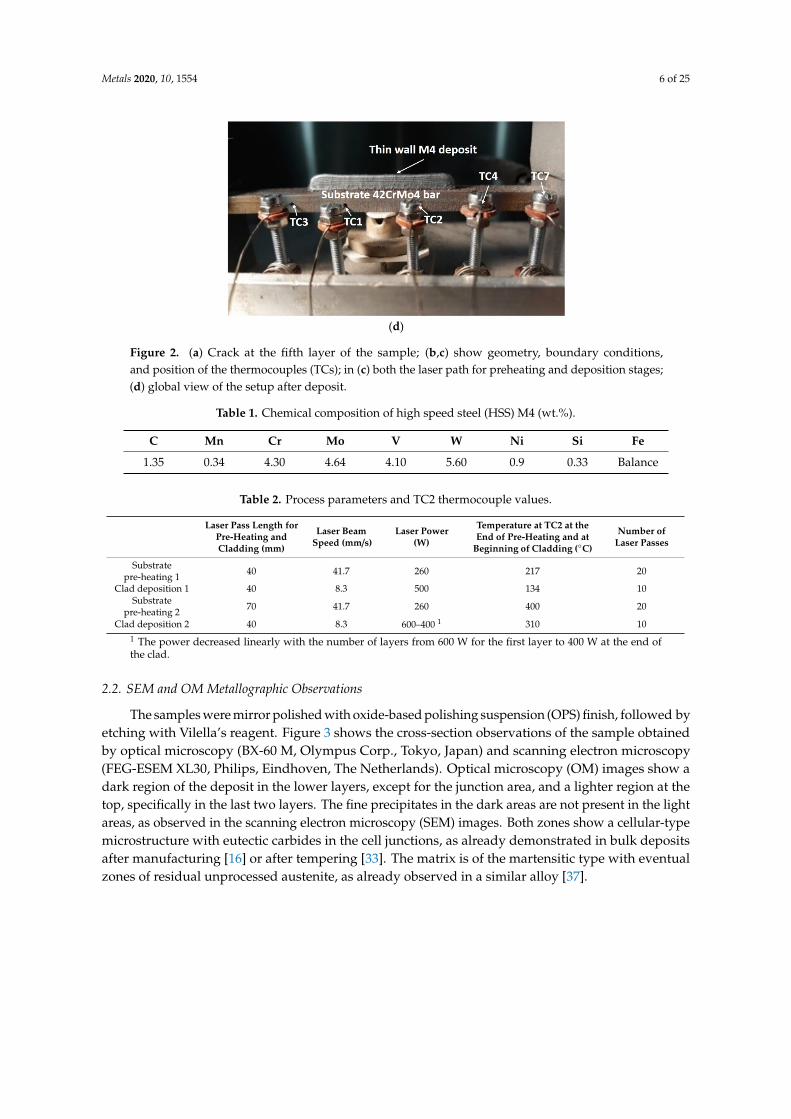
The composition of the HSS M4 commercial powder with its particle size ranging from 50 µm to150 µm is provided in Table 1. The 5-axis Laser Cladding system (IREPA LASER, Ilkirch, France) witha Nd-YAG laser of maximum power capacity of 2000 W from Sirris Research Centre (SIRRIS, Seraing,Belgium) is schematically described in Figure 1. The laser has a wavelength of 1064 µm and operatescontinuously. The metal powder is injected with an angle of 45 degrees. The laser has a top-hatenergy distribution with a mean diameter of 1500 µm (1400 µm at the top and 1600 µm at the bottom).The substrate consists of a small, rectangular bar of 8 mm height, 10 mm width, and 120 mm lengthof 42CrMo4 steel (Figure 2b). The bar supports are shown in Figure 2b while the thermocouple (TC)positions are given in Figure 2c. The preheating to prevent the crack appearance in the deposit wasperformed by preliminary laser passes (red line in Figure 2c). Preheating temperature values from217 ◦C to 400 ◦C were generated. For the lowest preheating temperature, cracks appeared during thedeposition of the fifth layer at the extremities of the substrate–clad interface (Figure 2a), but whenmanufactured with a preheating of 400 ◦C sound samples were achieved (Figure 2d). Table 2 givesthe process parameters of the simulated manufacturing cases. The final manufactured thin walls of40 × 4 × 1.5 mm3 were centered on the substrate top surface.

Metals 2020, 10, x FOR PEER REVIEW 5 of 24

2. Materials and Methods

2.1. Thin-Wall Experiments

The composition of the HSS M4 commercial powder with its particle size ranging from 50 µm to 150 µm is provided in Table 1. The 5-axis Laser Cladding system (IREPA LASER, Ilkirch, France) with a Nd-YAG laser of maximum power capacity of 2000 W from Sirris Research Centre (SIRRIS, Seraing, Belgium) is schematically described in Figure 1. The laser has a wavelength of 1064 µm and operates continuously. The metal powder is injected with an angle of 45 degrees. The laser has a top-hat energy distribution with a mean diameter of 1500 µm (1400 µm at the top and 1600 µm at the bottom). The substrate consists of a small, rectangular bar of 8 mm height, 10 mm width, and 120 mm length of 42CrMo4 steel (Figure 2b). The bar supports are shown in Figure 2b while the thermocouple (TC) positions are given in Figure 2c. The preheating to prevent the crack appearance in the deposit was performed by preliminary laser passes (red line in Figure 2c). Preheating temperature values from 217 °C to 400 °C were generated. For the lowest preheating temperature, cracks appeared during the deposition of the fifth layer at the extremities of the substrate–clad interface (Figure 2a), but when manufactured with a preheating of 400 °C sound samples were achieved (Figure 2d). Table 2 gives the process parameters of the simulated manufacturing cases. The final manufactured thin walls of 40 × 4 × 1.5 mm³ were centered on the substrate top surface.

(a)

(b)

(c)

Figure 2. Cont.

Metals 2020, 10, 1554 6 of 25

Metals 2020, 10, x FOR PEER REVIEW 6 of 24

(d)

Figure 2. (a) Crack at the fifth layer of the sample; (b,c) show geometry, boundary conditions, and position of the thermocouples (TCs); in (c) both the laser path for preheating and deposition stages; (d) global view of the setup after deposit.

Table 1. Chemical composition of high speed steel (HSS) M4 (wt.%).

C Mn Cr Mo V W Ni Si Fe 1.35 0.34 4.30 4.64 4.10 5.60 0.9 0.33 Balance

Table 2. Process parameters and TC2 thermocouple values.

Laser Pass Length for Pre-Heating and Cladding

(mm)

Laser Beam Speed (mm/s)

Laser Power

(W)

Temperature at TC2 at the End of Pre-Heating

and at Beginning of Cladding (°C)

Number of Laser

Passes

Substrate pre-heating 1

40 41.7 260 217 20

Clad deposition 1

40 8.3 500 134 10

Substrate pre-heating 2

70 41.7 260 400 20

Clad deposition 2

40 8.3 600–400 1 310 10

1 The power decreased linearly with the number of layers from 600 W for the first layer to 400 W at the end of the clad.

2.2. SEM and OM Metallographic Observations

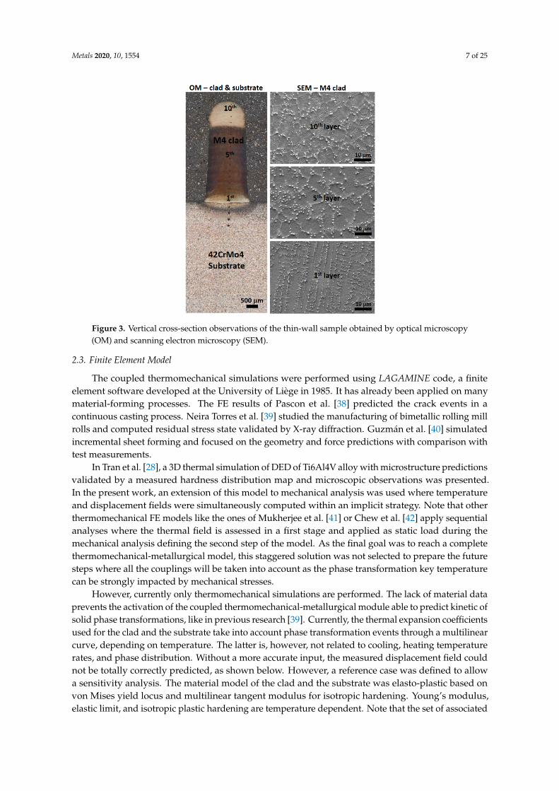
The samples were mirror polished with oxide-based polishing suspension (OPS) finish, followed by etching with Vilella’s reagent. Figure 3 shows the cross-section observations of the sample obtained by optical microscopy (BX-60 M, Olympus Corp., Tokyo, Japan) and scanning electron microscopy (FEG-ESEM XL30, Philips, Eindhoven, The Netherlands). Optical microscopy (OM) images show a dark region of the deposit in the lower layers, except for the junction area, and a lighter region at the top, specifically in the last two layers. The fine precipitates in the dark areas are not present in the light areas, as observed in the scanning electron microscopy (SEM) images. Both zones show a cellular-type microstructure with eutectic carbides in the cell junctions, as already demonstrated in bulk deposits after manufacturing [16] or after tempering [33]. The matrix is of the martensitic type with eventual zones of residual unprocessed austenite, as already observed in a similar alloy [37].

Figure 2. (a) Crack at the fifth layer of the sample; (b,c) show geometry, boundary conditions,and position of the thermocouples (TCs); in (c) both the laser path for preheating and deposition stages;(d) global view of the setup after deposit.

Table 1. Chemical composition of high speed steel (HSS) M4 (wt.%).

C Mn Cr Mo V W Ni Si Fe

1.35 0.34 4.30 4.64 4.10 5.60 0.9 0.33 Balance

Table 2. Process parameters and TC2 thermocouple values.

Laser Pass Length forPre-Heating andCladding (mm)

Laser BeamSpeed (mm/s)

Laser Power(W)

Temperature at TC2 at theEnd of Pre-Heating and at

Beginning of Cladding (◦C)

Number ofLaser Passes

Substratepre-heating 1 40 41.7 260 217 20

Clad deposition 1 40 8.3 500 134 10Substrate

pre-heating 2 70 41.7 260 400 20

Clad deposition 2 40 8.3 600–400 1 310 101 The power decreased linearly with the number of layers from 600 W for the first layer to 400 W at the end ofthe clad.

2.2. SEM and OM Metallographic Observations

The samples were mirror polished with oxide-based polishing suspension (OPS) finish, followed byetching with Vilella’s reagent. Figure 3 shows the cross-section observations of the sample obtainedby optical microscopy (BX-60 M, Olympus Corp., Tokyo, Japan) and scanning electron microscopy(FEG-ESEM XL30, Philips, Eindhoven, The Netherlands). Optical microscopy (OM) images show adark region of the deposit in the lower layers, except for the junction area, and a lighter region at thetop, specifically in the last two layers. The fine precipitates in the dark areas are not present in the lightareas, as observed in the scanning electron microscopy (SEM) images. Both zones show a cellular-typemicrostructure with eutectic carbides in the cell junctions, as already demonstrated in bulk depositsafter manufacturing [16] or after tempering [33]. The matrix is of the martensitic type with eventualzones of residual unprocessed austenite, as already observed in a similar alloy [37].

Metals 2020, 10, 1554 7 of 25

Metals 2020, 10, x FOR PEER REVIEW 7 of 24

Figure 3. Vertical cross-section observations of the thin-wall sample obtained by optical microscopy (OM) and scanning electron microscopy (SEM).

2.3. Finite Element Model

The coupled thermomechanical simulations were performed using LAGAMINE code, a finite element software developed at the University of Liège in 1985. It has already been applied on many material-forming processes. The FE results of Pascon et al. [38] predicted the crack events in a continuous casting process. Neira Torres et al. [39] studied the manufacturing of bimetallic rolling mill rolls and computed residual stress state validated by X-ray diffraction. Guzmán et al. [40] simulated incremental sheet forming and focused on the geometry and force predictions with comparison with test measurements.

In Tran et al. [28], a 3D thermal simulation of DED of Ti6Al4V alloy with microstructure predictions validated by a measured hardness distribution map and microscopic observations was presented. In the present work, an extension of this model to mechanical analysis was used where temperature and displacement fields were simultaneously computed within an implicit strategy. Note that other thermomechanical FE models like the ones of Mukherjee et al. [41] or Chew et al. [42] apply sequential analyses where the thermal field is assessed in a first stage and applied as static load during the mechanical analysis defining the second step of the model. As the final goal was to reach a complete thermomechanical-metallurgical model, this staggered solution was not selected to prepare the future steps where all the couplings will be taken into account as the phase transformation key temperature can be strongly impacted by mechanical stresses.

However, currently only thermomechanical simulations are performed. The lack of material data prevents the activation of the coupled thermomechanical-metallurgical module able to predict kinetic of solid phase transformations, like in previous research [39]. Currently, the thermal expansion coefficients used for the clad and the substrate take into account phase transformation events through a multilinear curve, depending on temperature. The latter is, however, not related to cooling, heating temperature rates, and phase distribution. Without a more accurate input, the measured displacement field could not be totally correctly predicted, as shown below. However, a reference case was defined to allow a sensitivity analysis. The material model of the clad and the substrate was elasto-plastic based on von Mises yield locus and multilinear tangent modulus for isotropic hardening. Young’s modulus, elastic limit, and isotropic plastic hardening are temperature dependent. Note that the set of associated tangent plastic moduli was kept constant for each curve.

Figure 3. Vertical cross-section observations of the thin-wall sample obtained by optical microscopy(OM) and scanning electron microscopy (SEM).

2.3. Finite Element Model

The coupled thermomechanical simulations were performed using LAGAMINE code, a finiteelement software developed at the University of Liège in 1985. It has already been applied on manymaterial-forming processes. The FE results of Pascon et al. [38] predicted the crack events in acontinuous casting process. Neira Torres et al. [39] studied the manufacturing of bimetallic rolling millrolls and computed residual stress state validated by X-ray diffraction. Guzmán et al. [40] simulatedincremental sheet forming and focused on the geometry and force predictions with comparison withtest measurements.

In Tran et al. [28], a 3D thermal simulation of DED of Ti6Al4V alloy with microstructure predictionsvalidated by a measured hardness distribution map and microscopic observations was presented.In the present work, an extension of this model to mechanical analysis was used where temperatureand displacement fields were simultaneously computed within an implicit strategy. Note that otherthermomechanical FE models like the ones of Mukherjee et al. [41] or Chew et al. [42] apply sequentialanalyses where the thermal field is assessed in a first stage and applied as static load during themechanical analysis defining the second step of the model. As the final goal was to reach a completethermomechanical-metallurgical model, this staggered solution was not selected to prepare the futuresteps where all the couplings will be taken into account as the phase transformation key temperaturecan be strongly impacted by mechanical stresses.

However, currently only thermomechanical simulations are performed. The lack of material dataprevents the activation of the coupled thermomechanical-metallurgical module able to predict kinetic ofsolid phase transformations, like in previous research [39]. Currently, the thermal expansion coefficientsused for the clad and the substrate take into account phase transformation events through a multilinearcurve, depending on temperature. The latter is, however, not related to cooling, heating temperaturerates, and phase distribution. Without a more accurate input, the measured displacement field couldnot be totally correctly predicted, as shown below. However, a reference case was defined to allowa sensitivity analysis. The material model of the clad and the substrate was elasto-plastic based onvon Mises yield locus and multilinear tangent modulus for isotropic hardening. Young’s modulus,elastic limit, and isotropic plastic hardening are temperature dependent. Note that the set of associated

Metals 2020, 10, 1554 8 of 25

tangent plastic moduli was kept constant for each curve. Besides, as low-viscosity effect was confirmedby the mechanical tests (Section 3), the strain hardening model was rate-insensitive.

The eight-node 3D brick (BWD3T) thermomechanical finite element implemented in theLagamine code by Zhu et al. [43] was selected. The element is based on the nonlinear, three-fieldHu-Washizuvariational principle of stress, strain, and displacement [44–46] and uses a mixedformulation adapted to large strains and large displacements with a reduced integration scheme—onlyone integration point—and an hourglass control technique.

The FE solid model simplified the physics of all the phenomena present in the melt pool. The effectof the latent heat of the fusion (Lf) was integrated in the definition of the thermal capacity (cp),defining an apparent property. The effect of the fluid motion due to the thermo-capillary phenomenon(i.e., Marangoni flow) was not considered. Other solid studies just consider a multiplicative factorto enhance the conductivity value within the melt pool [42,47]. Such a factor varies, according tothe research. For instance, Cao et al. [47] use a value of 3 for Ti6Al4V alloy while Bi et al. [48] use avalue of 5 for iron-based martensitic stainless-steel METCO 42C, respectively. Initially for welding,Lampa et al. [49] suggested a value of 2.5 for an austenitic stainless steel. Hereafter, following thearguments of Lindgren et al. [29], no multiplicative factor was applied as it counteracts the energydistribution defined in the heat source model. Clearly, such assumptions are not independent of thepowder laser absorptivity factor β, which is the current work numerically tuned within the simulations’process to agree with the observed melt pool size and the measured thermal history.

A second simplification consisted of the energy distribution of the heat flow of the laser. Whilethe model developed by Goldak defines a double ellipsoidal power density distribution [26], a simplecircular Gaussian is often considered [27,50]. The model considered in this present research waseven simpler: The mesh size was adapted to the laser spot radius. The clad finite cubic elementshad a 0.75 mm width to model the laser top-hat energy distribution with a diameter of 1.5 mm.As only half of the process was simulated by symmetry, and the final clad volume modeled was40.5 (length) × 0.75 (width) × 4 (height) mm3. Indeed, the mean height of the layers was measuredand corresponded to 0.4 mm. The effect of the moving laser beam was taken into account by updatingthe laser input power within the affected nodes, based on the real velocity and the trajectory of thelaser processing head.

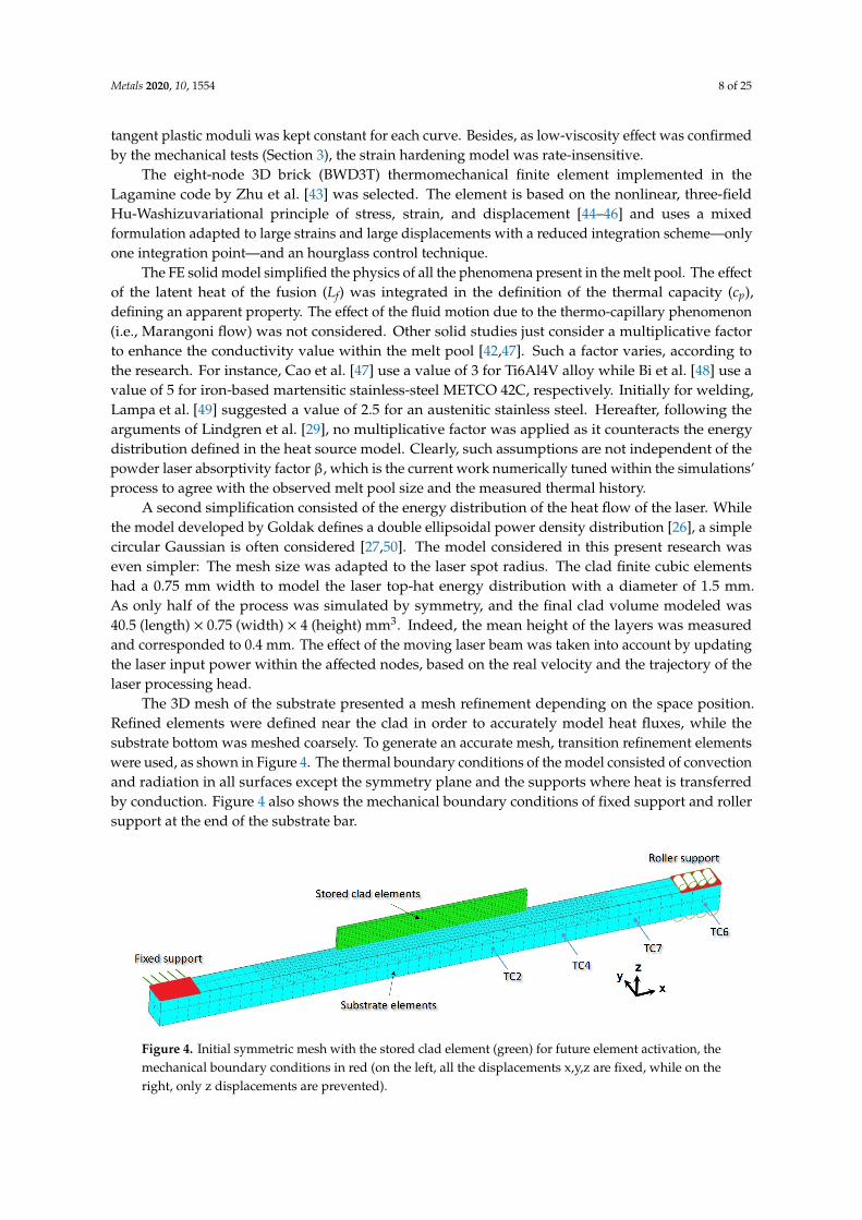
The 3D mesh of the substrate presented a mesh refinement depending on the space position.Refined elements were defined near the clad in order to accurately model heat fluxes, while thesubstrate bottom was meshed coarsely. To generate an accurate mesh, transition refinement elementswere used, as shown in Figure 4. The thermal boundary conditions of the model consisted of convectionand radiation in all surfaces except the symmetry plane and the supports where heat is transferredby conduction. Figure 4 also shows the mechanical boundary conditions of fixed support and rollersupport at the end of the substrate bar.

Metals 2020, 10, x FOR PEER REVIEW 8 of 24

Besides, as low-viscosity effect was confirmed by the mechanical tests (Section 3), the strain hardening model was rate-insensitive.

The eight-node 3D brick (BWD3T) thermomechanical finite element implemented in the Lagamine code by Zhu et al. [43] was selected. The element is based on the nonlinear, three-field Hu-Washizuvariational principle of stress, strain, and displacement [44–46] and uses a mixed formulation adapted to large strains and large displacements with a reduced integration scheme—only one integration point—and an hourglass control technique.

The FE solid model simplified the physics of all the phenomena present in the melt pool. The effect of the latent heat of the fusion (Lf) was integrated in the definition of the thermal capacity (cp), defining an apparent property. The effect of the fluid motion due to the thermo-capillary phenomenon (i.e., Marangoni flow) was not considered. Other solid studies just consider a multiplicative factor to enhance the conductivity value within the melt pool [42,47]. Such a factor varies, according to the research. For instance, Cao et al. [47] use a value of 3 for Ti6Al4V alloy while Bi et al. [48] use a value of 5 for iron-based martensitic stainless-steel METCO 42C, respectively. Initially for welding, Lampa et al. [49] suggested a value of 2.5 for an austenitic stainless steel. Hereafter, following the arguments of Lindgren et al. [29], no multiplicative factor was applied as it counteracts the energy distribution defined in the heat source model. Clearly, such assumptions are not independent of the powder laser absorptivity factor β, which is the current work numerically tuned within the simulations’ process to agree with the observed melt pool size and the measured thermal history.

A second simplification consisted of the energy distribution of the heat flow of the laser. While the model developed by Goldak defines a double ellipsoidal power density distribution [26], a simple circular Gaussian is often considered [27,50]. The model considered in this present research was even simpler: The mesh size was adapted to the laser spot radius. The clad finite cubic elements had a 0.75 mm width to model the laser top-hat energy distribution with a diameter of 1.5 mm. As only half of the process was simulated by symmetry, and the final clad volume modeled was 40.5 (length) × 0.75 (width) × 4 (height) mm³. Indeed, the mean height of the layers was measured and corresponded to 0.4 mm. The effect of the moving laser beam was taken into account by updating the laser input power within the affected nodes, based on the real velocity and the trajectory of the laser processing head.

The 3D mesh of the substrate presented a mesh refinement depending on the space position. Refined elements were defined near the clad in order to accurately model heat fluxes, while the substrate bottom was meshed coarsely. To generate an accurate mesh, transition refinement elements were used, as shown in Figure 4. The thermal boundary conditions of the model consisted of convection and radiation in all surfaces except the symmetry plane and the supports where heat is transferred by conduction. Figure 4 also shows the mechanical boundary conditions of fixed support and roller support at the end of the substrate bar.

Figure 4. Initial symmetric mesh with the stored clad element (green) for future element activation, the mechanical boundary conditions in red (on the left, all the displacements x,y,z are fixed, while on the right, only z displacements are prevented).

Figure 4. Initial symmetric mesh with the stored clad element (green) for future element activation, themechanical boundary conditions in red (on the left, all the displacements x,y,z are fixed, while on theright, only z displacements are prevented).

Metals 2020, 10, 1554 9 of 25

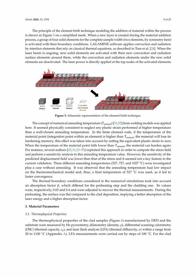
The principle of the element birth technique modeling the addition of material within the processis shown in Figure 5 on a simplified mesh. When a new layer is created during the material additionprocess, a group of four solid elements for the complete sample width (two elements, by symmetry here)is activated with their boundary conditions. LAGAMINE software applies convection and radiationby interface elements that rely on classical thermal equations, as described in Tran et al. [28]. When thelaser beam is ongoing, new solid elements are activated with their new convection and radiationsurface elements around them, while the convection and radiation elements under the new solidelements are deactivated. The laser power is directly applied at the top nodes of the activated elements.

Metals 2020, 10, x FOR PEER REVIEW 9 of 24

The principle of the element birth technique modeling the addition of material within the process is shown in Figure 5 on a simplified mesh. When a new layer is created during the material addition process, a group of four solid elements for the complete sample width (two elements, by symmetry here) is activated with their boundary conditions. LAGAMINE software applies convection and radiation by interface elements that rely on classical thermal equations, as described in Tran et al. [28]. When the laser beam is ongoing, new solid elements are activated with their new convection and radiation surface elements around them, while the convection and radiation elements under the new solid elements are deactivated. The laser power is directly applied at the top nodes of the activated elements.

Figure 5. Schematic representation of the element birth technique.

The concept of numerical annealing temperature (Tanneal) [51,52] from welding models was applied here. It seemed physically consistent to neglect any plastic strain performed at higher temperature than a well-chosen annealing temperature. In the finite element code, if the temperature of the material point (integration point within an element) is higher than Tanneal, the material will lose its hardening memory; this effect was taken into account by setting the equivalent plastic strain to zero. When the temperature of the material point falls lower than Tanneal, the material can harden again. For instance, several authors [25,31,53–55] exploited this approach in order to compute the stress field and perform a sensitivity analysis to this annealing temperature value. However, the sensitivity of the predicted displacement field was lower than that of the stress and it seemed not a key feature in the current validation. Three different annealing temperatures (527, 727, and 1027 °C) were investigated plus a case without annealing. It was observed that the annealing temperature had low impact on the thermomechanical model and, thus, a final temperature of 527 °C was used, as it led to faster convergence.

The thermal boundary conditions considered in the numerical simulations took into account an absorption factor β, which differed for the preheating step and the cladding one. Its values were, respectively, 0.65 and 0.4 and were adjusted to recover the thermal measurements. During the preheating, the surface was flat compared to the clad deposition, implying a better absorption of the laser energy and a higher absorption factor.

3. Material Parameters

3.1. Thermophysical Properties

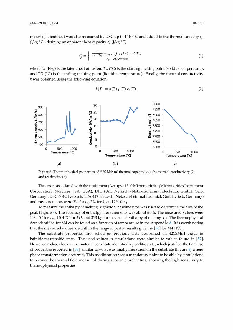
The thermophysical properties of the clad samples (Figure 6) manufactured by DED and the substrate were measured by He pycnometry, dilatometry (density, ρ), differential scanning calorimetry (DSC) (thermal capacity, cp), and laser flash analysis (LFA) (thermal diffusivity, α) within a range from 20 to 1100 °C (Appendix A). LFA measurements were carried out by steps of 100 °C. For the clad material, latent heat was also measured by DSC up to 1410 °C and added to the thermal capacity cp (J/kg °C), defining an apparent heat capacity 𝑐∗ (J/kg °C):

Figure 5. Schematic representation of the element birth technique.

The concept of numerical annealing temperature (Tanneal) [51,52] from welding models was appliedhere. It seemed physically consistent to neglect any plastic strain performed at higher temperaturethan a well-chosen annealing temperature. In the finite element code, if the temperature of thematerial point (integration point within an element) is higher than Tanneal, the material will lose itshardening memory; this effect was taken into account by setting the equivalent plastic strain to zero.When the temperature of the material point falls lower than Tanneal, the material can harden again.For instance, several authors [25,31,53–55] exploited this approach in order to compute the stress fieldand perform a sensitivity analysis to this annealing temperature value. However, the sensitivity of thepredicted displacement field was lower than that of the stress and it seemed not a key feature in thecurrent validation. Three different annealing temperatures (527, 727, and 1027 ◦C) were investigatedplus a case without annealing. It was observed that the annealing temperature had low impacton the thermomechanical model and, thus, a final temperature of 527 ◦C was used, as it led tofaster convergence.

The thermal boundary conditions considered in the numerical simulations took into accountan absorption factor β, which differed for the preheating step and the cladding one. Its valueswere, respectively, 0.65 and 0.4 and were adjusted to recover the thermal measurements. During thepreheating, the surface was flat compared to the clad deposition, implying a better absorption of thelaser energy and a higher absorption factor.

3. Material Parameters

3.1. Thermophysical Properties

The thermophysical properties of the clad samples (Figure 6) manufactured by DED and thesubstrate were measured by He pycnometry, dilatometry (density, ρ), differential scanning calorimetry(DSC) (thermal capacity, cp), and laser flash analysis (LFA) (thermal diffusivity, α) within a range from20 to 1100 ◦C (Appendix A). LFA measurements were carried out by steps of 100 ◦C. For the clad

Metals 2020, 10, 1554 10 of 25

material, latent heat was also measured by DSC up to 1410 ◦C and added to the thermal capacity cp

(J/kg ◦C), defining an apparent heat capacity c∗p (J/kg ◦C):

c∗p =

L fTD−Tm

+ cp, i f TD ≤ T ≤ Tm

cp, otherwise(1)

where L f (J/kg) is the latent heat of fusion, Tm (◦C) is the starting melting point (solidus temperature),and TD (◦C) is the ending melting point (liquidus temperature). Finally, the thermal conductivityk was obtained using the following equation:

k(T) = α(T)·ρ(T)·cp(T). (2)

Metals 2020, 10, x FOR PEER REVIEW 10 of 24

𝑐∗ 𝐿𝑇𝐷 𝑇 𝑐 , 𝑖𝑓 𝑇𝐷 T 𝑇 𝑐 , 𝑜𝑡ℎ𝑒𝑟𝑤𝑖𝑠𝑒 (1)

where 𝐿 (J/kg) is the latent heat of fusion, 𝑇 (°C) is the starting melting point (solidus temperature), and 𝑇𝐷 (°C) is the ending melting point (liquidus temperature). Finally, the thermal conductivity k was obtained using the following equation: 𝑘 𝑇 𝛼 𝑇 ∙ 𝜌 𝑇 ∙ 𝑐 𝑇 . (2)

The errors associated with the equipment (Accupyc 1340 Micromeritrics (Micromeritics Instrument Corporation, Norcross, GA, USA), DIL 402C Netzsch (Netzsch-Feinmahltechnick GmbH, Selb, Germany), DSC 404C Netzsch, LFA 427 Netzsch (Netzsch-Feinmahltechnick GmbH, Selb, Germany) and measurements were 3% for cp, 7% for k, and 2% for ρ.

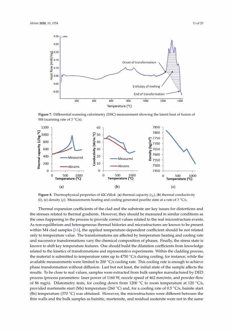
To measure the enthalpy of melting, sigmoidal baseline type was used to determine the area of the peak (Figure 7). The accuracy of enthalpy measurements was about ±5%. The measured values were 1230 °C for 𝑇 , 1404 °C for 𝑇𝐷 , and 313 J/g for the area of enthalpy of melting, 𝐿 . The thermophysical data identified for M4 can be found as a function of temperature in the Appendix A. It is worth noting that the measured values are within the range of partial results given in [56] for M4 HSS.

(a) (b) (c)

Figure 6. Thermophysical properties of HSS M4: (a) thermal capacity (cp), (b) thermal conductivity (k), and (c) density (ρ).

Figure 7. Differential scanning calorimetry (DSC) measurement showing the latent heat of fusion of M4 (scanning rate of 3 °C/s).

Figure 6. Thermophysical properties of HSS M4: (a) thermal capacity (cp), (b) thermal conductivity (k),and (c) density (ρ).

The errors associated with the equipment (Accupyc 1340 Micromeritrics (Micromeritics InstrumentCorporation, Norcross, GA, USA), DIL 402C Netzsch (Netzsch-Feinmahltechnick GmbH, Selb,Germany), DSC 404C Netzsch, LFA 427 Netzsch (Netzsch-Feinmahltechnick GmbH, Selb, Germany)and measurements were 3% for cp, 7% for k, and 2% for ρ.

To measure the enthalpy of melting, sigmoidal baseline type was used to determine the area of thepeak (Figure 7). The accuracy of enthalpy measurements was about ±5%. The measured values were1230 ◦C for Tm, 1404 ◦C for TD, and 313 J/g for the area of enthalpy of melting, L f . The thermophysicaldata identified for M4 can be found as a function of temperature in the Appendix A. It is worth notingthat the measured values are within the range of partial results given in [56] for M4 HSS.

The substrate properties first relied on previous tests performed on 42CrMo4 grade inbainitic-martensitic state. The used values in simulations were similar to values found in [57].However, a closer look at the material certificate identified a pearlitic state, which justified the final useof properties reported in [58], similar to what was finally measured on the substrate (Figure 8) wherephase transformation occurred. This modification was a mandatory point to be able by simulationsto recover the thermal field measured during substrate preheating, showing the high sensitivity tothermophysical properties.

Metals 2020, 10, 1554 11 of 25

Metals 2020, 10, x FOR PEER REVIEW 10 of 24

𝑐∗ 𝐿𝑇𝐷 𝑇 𝑐 , 𝑖𝑓 𝑇𝐷 T 𝑇 𝑐 , 𝑜𝑡ℎ𝑒𝑟𝑤𝑖𝑠𝑒 (1)

where 𝐿 (J/kg) is the latent heat of fusion, 𝑇 (°C) is the starting melting point (solidus temperature), and 𝑇𝐷 (°C) is the ending melting point (liquidus temperature). Finally, the thermal conductivity k was obtained using the following equation: 𝑘 𝑇 𝛼 𝑇 ∙ 𝜌 𝑇 ∙ 𝑐 𝑇 . (2)

The errors associated with the equipment (Accupyc 1340 Micromeritrics (Micromeritics Instrument Corporation, Norcross, GA, USA), DIL 402C Netzsch (Netzsch-Feinmahltechnick GmbH, Selb, Germany), DSC 404C Netzsch, LFA 427 Netzsch (Netzsch-Feinmahltechnick GmbH, Selb, Germany) and measurements were 3% for cp, 7% for k, and 2% for ρ.

To measure the enthalpy of melting, sigmoidal baseline type was used to determine the area of the peak (Figure 7). The accuracy of enthalpy measurements was about ±5%. The measured values were 1230 °C for 𝑇 , 1404 °C for 𝑇𝐷 , and 313 J/g for the area of enthalpy of melting, 𝐿 . The thermophysical data identified for M4 can be found as a function of temperature in the Appendix A. It is worth noting that the measured values are within the range of partial results given in [56] for M4 HSS.

(a) (b) (c)

Figure 6. Thermophysical properties of HSS M4: (a) thermal capacity (cp), (b) thermal conductivity (k), and (c) density (ρ).

Figure 7. Differential scanning calorimetry (DSC) measurement showing the latent heat of fusion of M4 (scanning rate of 3 °C/s). Figure 7. Differential scanning calorimetry (DSC) measurement showing the latent heat of fusion ofM4 (scanning rate of 3 ◦C/s).

Metals 2020, 10, x FOR PEER REVIEW 11 of 24

The substrate properties first relied on previous tests performed on 42CrMo4 grade in bainitic-martensitic state. The used values in simulations were similar to values found in [57]. However, a closer look at the material certificate identified a pearlitic state, which justified the final use of properties reported in [58], similar to what was finally measured on the substrate (Figure 8) where phase transformation occurred. This modification was a mandatory point to be able by simulations to recover the thermal field measured during substrate preheating, showing the high sensitivity to thermophysical properties.

(a) (b) (c)

Figure 8. Thermophysical properties of 42CrMo4: (a) thermal capacity (cp), (b) thermal conductivity (k), (c) density (ρ). Measurements heating and cooling generated pearlite state at a rate of 3 °C/s.

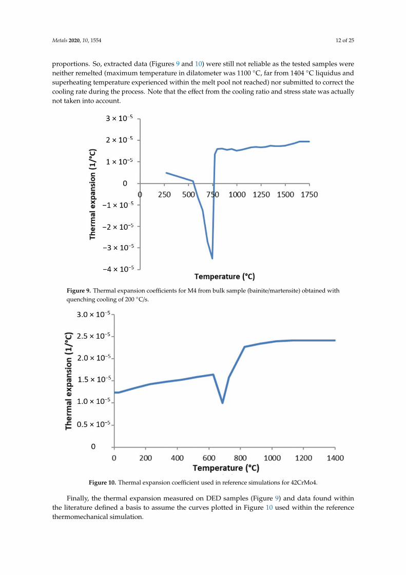
Thermal expansion coefficients of the clad and the substrate are key issues for distortions and the stresses related to thermal gradients. However, they should be measured in similar conditions as the ones happening in the process to provide correct values related to the real microstructure events. As non-equilibrium and heterogeneous thermal histories and microstructures are known to be present within M4 clad samples [16], the applied temperature-dependent coefficient should be not related only to temperature value. The transformations are affected by temperature heating and cooling rate and successive transformations vary the chemical composition of phases. Finally, the stress state is known to shift key temperature features. One should build the dilatation coefficients from knowledge related to the kinetics of transformations and representative experiments. Within the cladding process, the material is submitted to temperature rates up to 4750 °C/s during cooling, for instance, while the available measurements were limited to 200 °C/s cooling rate. This cooling rate is enough to achieve phase transformation without diffusion. Last but not least, the initial state of the sample affects the results. To be close to real values, samples were extracted from bulk samples manufactured by DED process (process parameters: laser power of 1160 W, nozzle speed of 462 mm/min, and powder flow of 86 mg/s). Dilatometry tests, for cooling down from 1200 °C to room temperature at 120 °C/sec, provided martensite start (Ms) temperature (260 °C) and, for a cooling rate of 0.5 °C/s, bainite start (Bs) temperature (370 °C) was obtained. However, the microstructures were different between the thin walls and the bulk samples as bainitic, martensite, and residual austenite were not in the same proportions. So, extracted data (Figures 9 and 10) were still not reliable as the tested samples were neither remelted (maximum temperature in dilatometer was 1100 °C, far from 1404 °C liquidus and superheating temperature experienced within the melt pool not reached) nor submitted to correct the cooling rate during the process. Note that the effect from the cooling ratio and stress state was actually not taken into account.

Finally, the thermal expansion measured on DED samples (Figure 9) and data found within the literature defined a basis to assume the curves plotted in Figure 10 used within the reference thermomechanical simulation.

Figure 8. Thermophysical properties of 42CrMo4: (a) thermal capacity (cp), (b) thermal conductivity(k), (c) density (ρ). Measurements heating and cooling generated pearlite state at a rate of 3 ◦C/s.

Thermal expansion coefficients of the clad and the substrate are key issues for distortions andthe stresses related to thermal gradients. However, they should be measured in similar conditions asthe ones happening in the process to provide correct values related to the real microstructure events.As non-equilibrium and heterogeneous thermal histories and microstructures are known to be presentwithin M4 clad samples [16], the applied temperature-dependent coefficient should be not relatedonly to temperature value. The transformations are affected by temperature heating and cooling rateand successive transformations vary the chemical composition of phases. Finally, the stress state isknown to shift key temperature features. One should build the dilatation coefficients from knowledgerelated to the kinetics of transformations and representative experiments. Within the cladding process,the material is submitted to temperature rates up to 4750 ◦C/s during cooling, for instance, while theavailable measurements were limited to 200 ◦C/s cooling rate. This cooling rate is enough to achievephase transformation without diffusion. Last but not least, the initial state of the sample affects theresults. To be close to real values, samples were extracted from bulk samples manufactured by DEDprocess (process parameters: laser power of 1160 W, nozzle speed of 462 mm/min, and powder flowof 86 mg/s). Dilatometry tests, for cooling down from 1200 ◦C to room temperature at 120 ◦C/s,provided martensite start (Ms) temperature (260 ◦C) and, for a cooling rate of 0.5 ◦C/s, bainite start(Bs) temperature (370 ◦C) was obtained. However, the microstructures were different between thethin walls and the bulk samples as bainitic, martensite, and residual austenite were not in the same

Metals 2020, 10, 1554 12 of 25

proportions. So, extracted data (Figures 9 and 10) were still not reliable as the tested samples wereneither remelted (maximum temperature in dilatometer was 1100 ◦C, far from 1404 ◦C liquidus andsuperheating temperature experienced within the melt pool not reached) nor submitted to correct thecooling rate during the process. Note that the effect from the cooling ratio and stress state was actuallynot taken into account.

Figure 9. Thermal expansion coefficients for M4 from bulk sample (bainite/martensite) obtained withquenching cooling of 200 ◦C/s.

Figure 10. Thermal expansion coefficient used in reference simulations for 42CrMo4.

Finally, the thermal expansion measured on DED samples (Figure 9) and data found withinthe literature defined a basis to assume the curves plotted in Figure 10 used within the referencethermomechanical simulation.

Metals 2020, 10, 1554 13 of 25

Note that those thermal dilatation coefficients (α) follow the classical metallurgist definition of:

α(T) = (1/L0)(LT − L0)/(T − T0) (3)

where L is the length, T is the temperature and index 0 means at room temperature.

3.2. Stress–Strain Curves

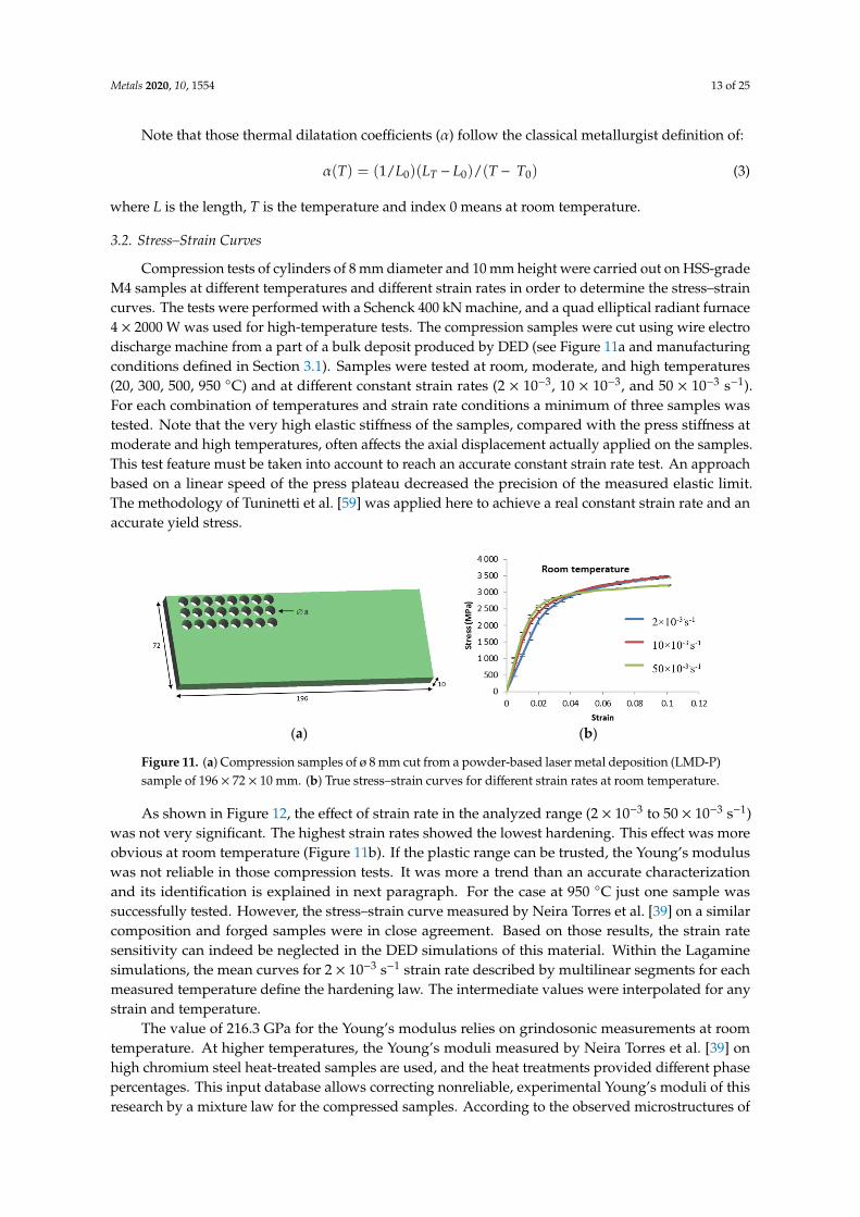
Compression tests of cylinders of 8 mm diameter and 10 mm height were carried out on HSS-gradeM4 samples at different temperatures and different strain rates in order to determine the stress–straincurves. The tests were performed with a Schenck 400 kN machine, and a quad elliptical radiant furnace4 × 2000 W was used for high-temperature tests. The compression samples were cut using wire electrodischarge machine from a part of a bulk deposit produced by DED (see Figure 11a and manufacturingconditions defined in Section 3.1). Samples were tested at room, moderate, and high temperatures(20, 300, 500, 950 ◦C) and at different constant strain rates (2 × 10−3, 10 × 10−3, and 50 × 10−3 s−1).For each combination of temperatures and strain rate conditions a minimum of three samples wastested. Note that the very high elastic stiffness of the samples, compared with the press stiffness atmoderate and high temperatures, often affects the axial displacement actually applied on the samples.This test feature must be taken into account to reach an accurate constant strain rate test. An approachbased on a linear speed of the press plateau decreased the precision of the measured elastic limit.The methodology of Tuninetti et al. [59] was applied here to achieve a real constant strain rate and anaccurate yield stress.Metals 2020, 10, x FOR PEER REVIEW 13 of 24

(a) (b)

Figure 11. (a) Compression samples of ø 8 mm cut from a powder-based laser metal deposition (LMD-P) sample of 196 × 72 × 10 mm. (b) True stress–strain curves for different strain rates at room temperature.

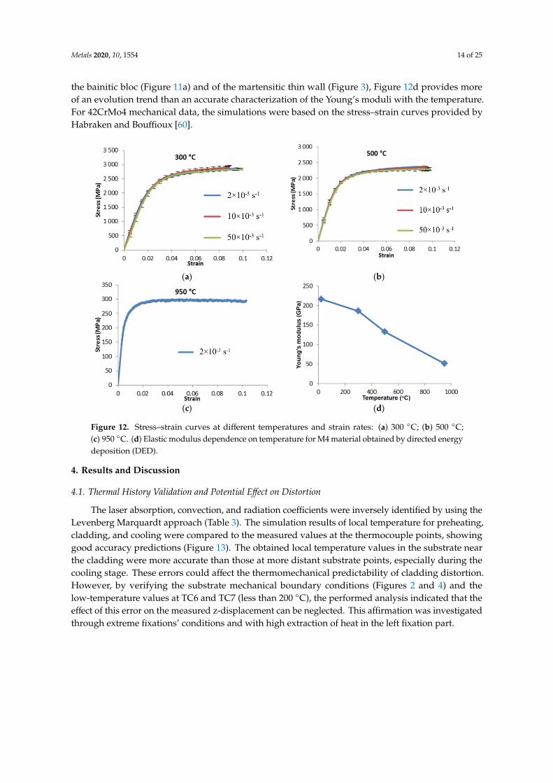
As shown in Figure 12, the effect of strain rate in the analyzed range (2 × 10–3 to 50 × 10–3 s–1) was not very significant. The highest strain rates showed the lowest hardening. This effect was more obvious at room temperature (Figure 11b). If the plastic range can be trusted, the Young’s modulus was not reliable in those compression tests. It was more a trend than an accurate characterization and its identification is explained in next paragraph. For the case at 950 °C just one sample was successfully tested. However, the stress–strain curve measured by Neira Torres et al. [39] on a similar composition and forged samples were in close agreement. Based on those results, the strain rate sensitivity can indeed be neglected in the DED simulations of this material. Within the Lagamine simulations, the mean curves for 2 × 10–3 s–1 strain rate described by multilinear segments for each measured temperature define the hardening law. The intermediate values were interpolated for any strain and temperature.

(a) (b)

(c) (d)

Figure 12. Stress–strain curves at different temperatures and strain rates: (a) 300 °C; (b) 500 °C; (c) 950 °C. (d) Elastic modulus dependence on temperature for M4 material obtained by directed energy deposition (DED).

Figure 11. (a) Compression samples of ø 8 mm cut from a powder-based laser metal deposition (LMD-P)sample of 196 × 72 × 10 mm. (b) True stress–strain curves for different strain rates at room temperature.

As shown in Figure 12, the effect of strain rate in the analyzed range (2 × 10−3 to 50 × 10−3 s−1)was not very significant. The highest strain rates showed the lowest hardening. This effect was moreobvious at room temperature (Figure 11b). If the plastic range can be trusted, the Young’s moduluswas not reliable in those compression tests. It was more a trend than an accurate characterizationand its identification is explained in next paragraph. For the case at 950 ◦C just one sample wassuccessfully tested. However, the stress–strain curve measured by Neira Torres et al. [39] on a similarcomposition and forged samples were in close agreement. Based on those results, the strain ratesensitivity can indeed be neglected in the DED simulations of this material. Within the Lagaminesimulations, the mean curves for 2 × 10−3 s−1 strain rate described by multilinear segments for eachmeasured temperature define the hardening law. The intermediate values were interpolated for anystrain and temperature.

The value of 216.3 GPa for the Young’s modulus relies on grindosonic measurements at roomtemperature. At higher temperatures, the Young’s moduli measured by Neira Torres et al. [39] onhigh chromium steel heat-treated samples are used, and the heat treatments provided different phasepercentages. This input database allows correcting nonreliable, experimental Young’s moduli of thisresearch by a mixture law for the compressed samples. According to the observed microstructures of

Metals 2020, 10, 1554 14 of 25

the bainitic bloc (Figure 11a) and of the martensitic thin wall (Figure 3), Figure 12d provides moreof an evolution trend than an accurate characterization of the Young’s moduli with the temperature.For 42CrMo4 mechanical data, the simulations were based on the stress–strain curves provided byHabraken and Bouffioux [60].

Metals 2020, 10, x FOR PEER REVIEW 13 of 24

(a) (b)

Figure 11. (a) Compression samples of ø 8 mm cut from a powder-based laser metal deposition (LMD-P) sample of 196 × 72 × 10 mm. (b) True stress–strain curves for different strain rates at room temperature.

As shown in Figure 12, the effect of strain rate in the analyzed range (2 × 10–3 to 50 × 10–3 s–1) was not very significant. The highest strain rates showed the lowest hardening. This effect was more obvious at room temperature (Figure 11b). If the plastic range can be trusted, the Young’s modulus was not reliable in those compression tests. It was more a trend than an accurate characterization and its identification is explained in next paragraph. For the case at 950 °C just one sample was successfully tested. However, the stress–strain curve measured by Neira Torres et al. [39] on a similar composition and forged samples were in close agreement. Based on those results, the strain rate sensitivity can indeed be neglected in the DED simulations of this material. Within the Lagamine simulations, the mean curves for 2 × 10–3 s–1 strain rate described by multilinear segments for each measured temperature define the hardening law. The intermediate values were interpolated for any strain and temperature.

(a) (b)

(c) (d)

Figure 12. Stress–strain curves at different temperatures and strain rates: (a) 300 °C; (b) 500 °C; (c) 950 °C. (d) Elastic modulus dependence on temperature for M4 material obtained by directed energy deposition (DED).

Figure 12. Stress–strain curves at different temperatures and strain rates: (a) 300 ◦C; (b) 500 ◦C;(c) 950 ◦C. (d) Elastic modulus dependence on temperature for M4 material obtained by directed energydeposition (DED).

4. Results and Discussion

4.1. Thermal History Validation and Potential Effect on Distortion

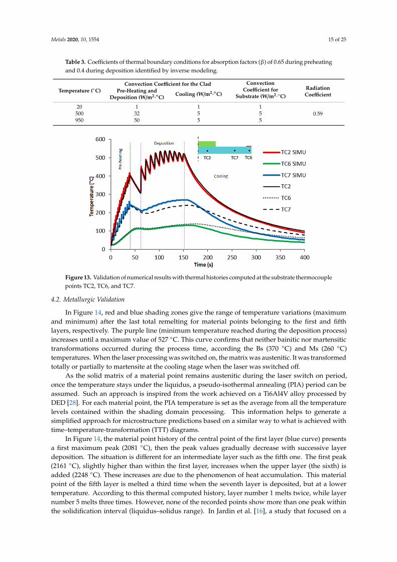
The laser absorption, convection, and radiation coefficients were inversely identified by using theLevenberg Marquardt approach (Table 3). The simulation results of local temperature for preheating,cladding, and cooling were compared to the measured values at the thermocouple points, showinggood accuracy predictions (Figure 13). The obtained local temperature values in the substrate nearthe cladding were more accurate than those at more distant substrate points, especially during thecooling stage. These errors could affect the thermomechanical predictability of cladding distortion.However, by verifying the substrate mechanical boundary conditions (Figures 2 and 4) and thelow-temperature values at TC6 and TC7 (less than 200 ◦C), the performed analysis indicated that theeffect of this error on the measured z-displacement can be neglected. This affirmation was investigatedthrough extreme fixations’ conditions and with high extraction of heat in the left fixation part.

Metals 2020, 10, 1554 15 of 25

Table 3. Coefficients of thermal boundary conditions for absorption factors (β) of 0.65 during preheatingand 0.4 during deposition identified by inverse modeling.

Temperature (◦C)Convection Coefficient for the Clad Convection

Coefficient forSubstrate (W/m2

·◦C)

RadiationCoefficient

Pre-Heating andDeposition (W/m2·◦C) Cooling (W/m2·◦C)

20 1 1 10.59500 32 5 5

950 50 5 5

Metals 2020, 10, x FOR PEER REVIEW 14 of 24

The value of 216.3 GPa for the Young’s modulus relies on grindosonic measurements at room temperature. At higher temperatures, the Young’s moduli measured by Neira Torres et al. [39] on high chromium steel heat-treated samples are used, and the heat treatments provided different phase percentages. This input database allows correcting nonreliable, experimental Young’s moduli of this research by a mixture law for the compressed samples. According to the observed microstructures of the bainitic bloc (Figure 11a) and of the martensitic thin wall (Figure 3), Figure 12d provides more of an evolution trend than an accurate characterization of the Young’s moduli with the temperature. For 42CrMo4 mechanical data, the simulations were based on the stress–strain curves provided by Habraken and Bouffioux [60].

4. Results and Discussion

4.1. Thermal History Validation and Potential Effect on Distortion

The laser absorption, convection, and radiation coefficients were inversely identified by using the Levenberg Marquardt approach (Table 3). The simulation results of local temperature for preheating, cladding, and cooling were compared to the measured values at the thermocouple points, showing good accuracy predictions (Figure 13). The obtained local temperature values in the substrate near the cladding were more accurate than those at more distant substrate points, especially during the cooling stage. These errors could affect the thermomechanical predictability of cladding distortion. However, by verifying the substrate mechanical boundary conditions (Figures 2 and 4) and the low-temperature values at TC6 and TC7 (less than 200 °C), the performed analysis indicated that the effect of this error on the measured z-displacement can be neglected. This affirmation was investigated through extreme fixations’ conditions and with high extraction of heat in the left fixation part.

Table 3. Coefficients of thermal boundary conditions for absorption factors (β) of 0.65 during preheating and 0.4 during deposition identified by inverse modeling.

Temperature (°C)

Convection Coefficient for the Clad Convection Coefficient for

Substrate (W/m²·°C)

Radiation Coefficient

Pre-Heating and Deposition (W/m²·°C)

Cooling (W/m²·°C)

20 1 1 1 0.59 500 32 5 5

950 50 5 5

Figure 13. Validation of numerical results with thermal histories computed at the substrate thermocouple points TC2, TC6, and TC7. Figure 13. Validation of numerical results with thermal histories computed at the substrate thermocouplepoints TC2, TC6, and TC7.

4.2. Metallurgic Validation

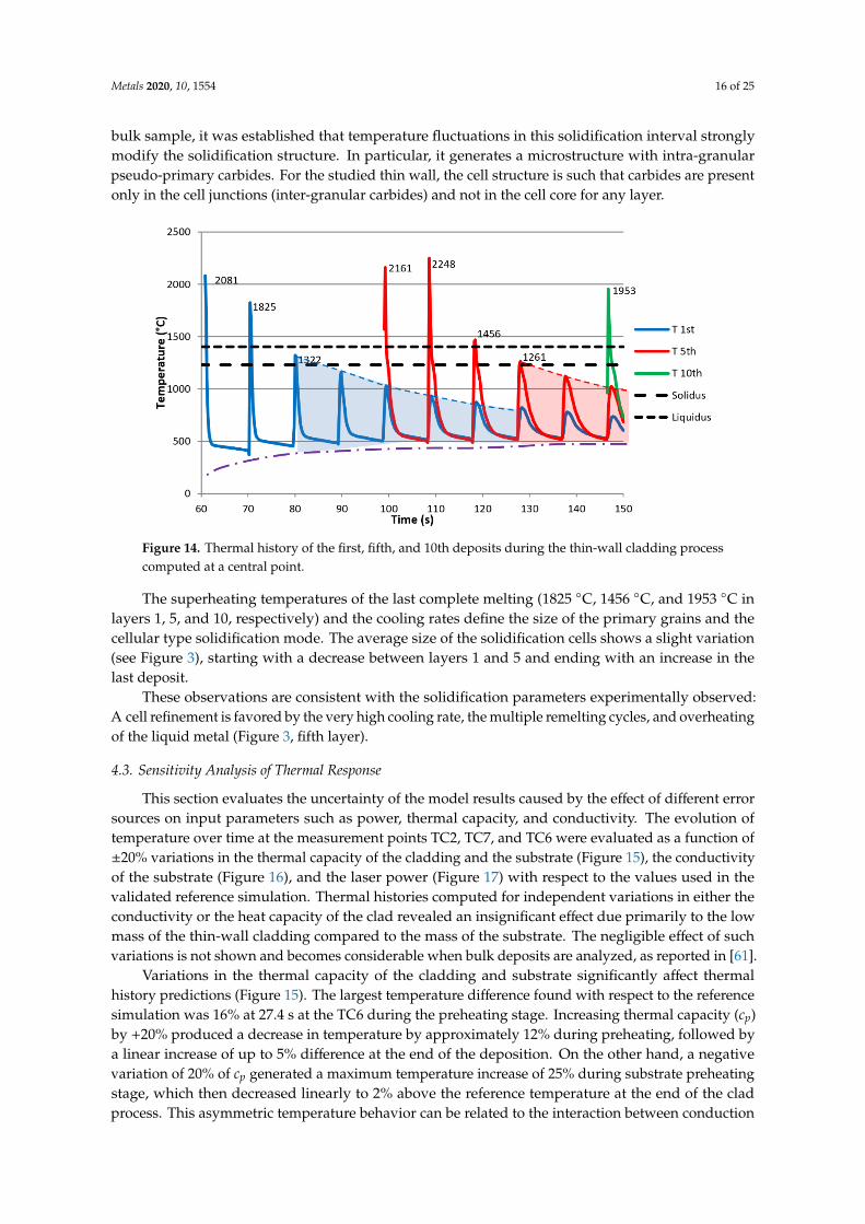
In Figure 14, red and blue shading zones give the range of temperature variations (maximumand minimum) after the last total remelting for material points belonging to the first and fifthlayers, respectively. The purple line (minimum temperature reached during the deposition process)increases until a maximum value of 527 ◦C. This curve confirms that neither bainitic nor martensitictransformations occurred during the process time, according the Bs (370 ◦C) and Ms (260 ◦C)temperatures. When the laser processing was switched on, the matrix was austenitic. It was transformedtotally or partially to martensite at the cooling stage when the laser was switched off.

As the solid matrix of a material point remains austenitic during the laser switch on period,once the temperature stays under the liquidus, a pseudo-isothermal annealing (PIA) period can beassumed. Such an approach is inspired from the work achieved on a Ti6Al4V alloy processed byDED [28]. For each material point, the PIA temperature is set as the average from all the temperaturelevels contained within the shading domain processing. This information helps to generate asimplified approach for microstructure predictions based on a similar way to what is achieved withtime–temperature-transformation (TTT) diagrams.

In Figure 14, the material point history of the central point of the first layer (blue curve) presentsa first maximum peak (2081 ◦C), then the peak values gradually decrease with successive layerdeposition. The situation is different for an intermediate layer such as the fifth one. The first peak(2161 ◦C), slightly higher than within the first layer, increases when the upper layer (the sixth) isadded (2248 ◦C). These increases are due to the phenomenon of heat accumulation. This materialpoint of the fifth layer is melted a third time when the seventh layer is deposited, but at a lowertemperature. According to this thermal computed history, layer number 1 melts twice, while layernumber 5 melts three times. However, none of the recorded points show more than one peak withinthe solidification interval (liquidus–solidus range). In Jardin et al. [16], a study that focused on a

Metals 2020, 10, 1554 16 of 25

bulk sample, it was established that temperature fluctuations in this solidification interval stronglymodify the solidification structure. In particular, it generates a microstructure with intra-granularpseudo-primary carbides. For the studied thin wall, the cell structure is such that carbides are presentonly in the cell junctions (inter-granular carbides) and not in the cell core for any layer.

Metals 2020, 10, x FOR PEER REVIEW 15 of 24

4.2. Metallurgic Validation

In Figure 14, red and blue shading zones give the range of temperature variations (maximum and minimum) after the last total remelting for material points belonging to the first and fifth layers, respectively. The purple line (minimum temperature reached during the deposition process) increases until a maximum value of 527 °C. This curve confirms that neither bainitic nor martensitic transformations occurred during the process time, according the Bs (370 °C) and Ms (260 °C) temperatures. When the laser processing was switched on, the matrix was austenitic. It was transformed totally or partially to martensite at the cooling stage when the laser was switched off.

Figure 14. Thermal history of the first, fifth, and 10th deposits during the thin-wall cladding process computed at a central point.

As the solid matrix of a material point remains austenitic during the laser switch on period, once the temperature stays under the liquidus, a pseudo-isothermal annealing (PIA) period can be assumed. Such an approach is inspired from the work achieved on a Ti6Al4V alloy processed by DED [28]. For each material point, the PIA temperature is set as the average from all the temperature levels contained within the shading domain processing. This information helps to generate a simplified approach for microstructure predictions based on a similar way to what is achieved with time–temperature-transformation (TTT) diagrams.

In Figure 14, the material point history of the central point of the first layer (blue curve) presents a first maximum peak (2081 °C), then the peak values gradually decrease with successive layer deposition. The situation is different for an intermediate layer such as the fifth one. The first peak (2161 °C), slightly higher than within the first layer, increases when the upper layer (the sixth) is added (2248 °C). These increases are due to the phenomenon of heat accumulation. This material point of the fifth layer is melted a third time when the seventh layer is deposited, but at a lower temperature. According to this thermal computed history, layer number 1 melts twice, while layer number 5 melts three times. However, none of the recorded points show more than one peak within the solidification interval (liquidus–solidus range). In Jardin et al. [16], a study that focused on a bulk sample, it was established that temperature fluctuations in this solidification interval strongly modify the solidification structure. In particular, it generates a microstructure with intra-granular pseudo-primary carbides. For the studied thin wall, the cell structure is such that carbides are present only in the cell junctions (inter-granular carbides) and not in the cell core for any layer.

The superheating temperatures of the last complete melting (1825 °C, 1456 °C, and 1953 °C in layers 1, 5, and 10, respectively) and the cooling rates define the size of the primary grains and the cellular type solidification mode. The average size of the solidification cells shows a slight variation

Figure 14. Thermal history of the first, fifth, and 10th deposits during the thin-wall cladding processcomputed at a central point.

The superheating temperatures of the last complete melting (1825 ◦C, 1456 ◦C, and 1953 ◦C inlayers 1, 5, and 10, respectively) and the cooling rates define the size of the primary grains and thecellular type solidification mode. The average size of the solidification cells shows a slight variation(see Figure 3), starting with a decrease between layers 1 and 5 and ending with an increase in thelast deposit.

These observations are consistent with the solidification parameters experimentally observed:A cell refinement is favored by the very high cooling rate, the multiple remelting cycles, and overheatingof the liquid metal (Figure 3, fifth layer).

4.3. Sensitivity Analysis of Thermal Response

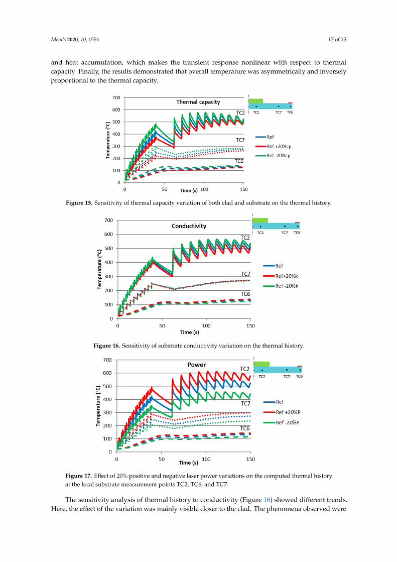
This section evaluates the uncertainty of the model results caused by the effect of different errorsources on input parameters such as power, thermal capacity, and conductivity. The evolution oftemperature over time at the measurement points TC2, TC7, and TC6 were evaluated as a function of±20% variations in the thermal capacity of the cladding and the substrate (Figure 15), the conductivityof the substrate (Figure 16), and the laser power (Figure 17) with respect to the values used in thevalidated reference simulation. Thermal histories computed for independent variations in either theconductivity or the heat capacity of the clad revealed an insignificant effect due primarily to the lowmass of the thin-wall cladding compared to the mass of the substrate. The negligible effect of suchvariations is not shown and becomes considerable when bulk deposits are analyzed, as reported in [61].

Variations in the thermal capacity of the cladding and substrate significantly affect thermalhistory predictions (Figure 15). The largest temperature difference found with respect to the referencesimulation was 16% at 27.4 s at the TC6 during the preheating stage. Increasing thermal capacity (cp)by +20% produced a decrease in temperature by approximately 12% during preheating, followed bya linear increase of up to 5% difference at the end of the deposition. On the other hand, a negativevariation of 20% of cp generated a maximum temperature increase of 25% during substrate preheatingstage, which then decreased linearly to 2% above the reference temperature at the end of the cladprocess. This asymmetric temperature behavior can be related to the interaction between conduction

Metals 2020, 10, 1554 17 of 25

and heat accumulation, which makes the transient response nonlinear with respect to thermalcapacity. Finally, the results demonstrated that overall temperature was asymmetrically and inverselyproportional to the thermal capacity.

Metals 2020, 10, x FOR PEER REVIEW 16 of 24

(see Figure 3), starting with a decrease between layers 1 and 5 and ending with an increase in the last deposit.

These observations are consistent with the solidification parameters experimentally observed: A cell refinement is favored by the very high cooling rate, the multiple remelting cycles, and overheating of the liquid metal (Figure 3, fifth layer).

4.3. Sensitivity Analysis of Thermal Response

This section evaluates the uncertainty of the model results caused by the effect of different error sources on input parameters such as power, thermal capacity, and conductivity. The evolution of temperature over time at the measurement points TC2, TC7, and TC6 were evaluated as a function of ±20% variations in the thermal capacity of the cladding and the substrate (Figure 15), the conductivity of the substrate (Figure 16), and the laser power (Figure 17) with respect to the values used in the validated reference simulation. Thermal histories computed for independent variations in either the conductivity or the heat capacity of the clad revealed an insignificant effect due primarily to the low mass of the thin-wall cladding compared to the mass of the substrate. The negligible effect of such variations is not shown and becomes considerable when bulk deposits are analyzed, as reported in [61].

Figure 15. Sensitivity of thermal capacity variation of both clad and substrate on the thermal history.

Figure 16. Sensitivity of substrate conductivity variation on the thermal history.

Figure 15. Sensitivity of thermal capacity variation of both clad and substrate on the thermal history.

Metals 2020, 10, x FOR PEER REVIEW 16 of 24

(see Figure 3), starting with a decrease between layers 1 and 5 and ending with an increase in the last deposit.

These observations are consistent with the solidification parameters experimentally observed: A cell refinement is favored by the very high cooling rate, the multiple remelting cycles, and overheating of the liquid metal (Figure 3, fifth layer).

4.3. Sensitivity Analysis of Thermal Response

This section evaluates the uncertainty of the model results caused by the effect of different error sources on input parameters such as power, thermal capacity, and conductivity. The evolution of temperature over time at the measurement points TC2, TC7, and TC6 were evaluated as a function of ±20% variations in the thermal capacity of the cladding and the substrate (Figure 15), the conductivity of the substrate (Figure 16), and the laser power (Figure 17) with respect to the values used in the validated reference simulation. Thermal histories computed for independent variations in either the conductivity or the heat capacity of the clad revealed an insignificant effect due primarily to the low mass of the thin-wall cladding compared to the mass of the substrate. The negligible effect of such variations is not shown and becomes considerable when bulk deposits are analyzed, as reported in [61].

Figure 15. Sensitivity of thermal capacity variation of both clad and substrate on the thermal history.

Figure 16. Sensitivity of substrate conductivity variation on the thermal history. Figure 16. Sensitivity of substrate conductivity variation on the thermal history.Metals 2020, 10, x FOR PEER REVIEW 17 of 24

Figure 17. Effect of 20% positive and negative laser power variations on the computed thermal history at the local substrate measurement points TC2, TC6, and TC7.

Variations in the thermal capacity of the cladding and substrate significantly affect thermal history predictions (Figure 15). The largest temperature difference found with respect to the reference simulation was 16% at 27.4 s at the TC6 during the preheating stage. Increasing thermal capacity (cp) by +20% produced a decrease in temperature by approximately 12% during preheating, followed by a linear increase of up to 5% difference at the end of the deposition. On the other hand, a negative variation of 20% of cp generated a maximum temperature increase of 25% during substrate preheating stage, which then decreased linearly to 2% above the reference temperature at the end of the clad process. This asymmetric temperature behavior can be related to the interaction between conduction and heat accumulation, which makes the transient response nonlinear with respect to thermal capacity. Finally, the results demonstrated that overall temperature was asymmetrically and inversely proportional to the thermal capacity.

The sensitivity analysis of thermal history to conductivity (Figure 16) showed different trends. Here, the effect of the variation was mainly visible closer to the clad. The phenomena observed were expected because, with an increased conductivity, heat propagates more easily in the substrate. There is less heat concentration close to the deposit (hence, lower temperature), and far from the deposit there is more heat transmission before being lost by convection and radiation. Conversely, lower conductivity increases the temperature near the cladding zone because more heat is transferred from the free surface of the substrate to the environment. This latter behavior is consistent with the lumped heat capacity of the substrate, where internal resistance to heat transfer becomes negligible in comparison to the external resistance of convection and radiation. This fact also explains the small effect of conductivity on temperature variations at TC7 and TC6 points located far from the clad. From Figures 15 and 16, it can be concluded that the thermal history of the thin wall of HSS is more sensitive to thermal capacity than to conductivity.

Global sensitivity analysis of power (Figure 17) on thermal history is self-explicative. Results show that increase in power leads to an increase of temperature and vice versa. Such high sensitivity helps to get an easy identification of absorption coefficient.

4.4. Sensitivity Analysis of Thermomechanical Response

The identified evolution of thermal expansion coefficients of the clad and the substrate (Figures 9 and 10) are essential and highly influential for determining the behavior of deformation and stress fields. However, these coefficient values strongly vary with the phase transformation kinetics of both materials. The impact of these phase transformations was not assessed in this article, as that would necessitate the need to include a metallurgical model. Currently, metallurgical data and models for very high heating and cooling rates for high speed steel are lacking. Thus, in a pragmatic exploratory research, the assumed average thermal expansion curves of Figure 10 were kept the same and just the impacts of the Young’s modulus and the yield stress accuracy were investigated.

Figure 17. Effect of 20% positive and negative laser power variations on the computed thermal historyat the local substrate measurement points TC2, TC6, and TC7.

The sensitivity analysis of thermal history to conductivity (Figure 16) showed different trends.Here, the effect of the variation was mainly visible closer to the clad. The phenomena observed were

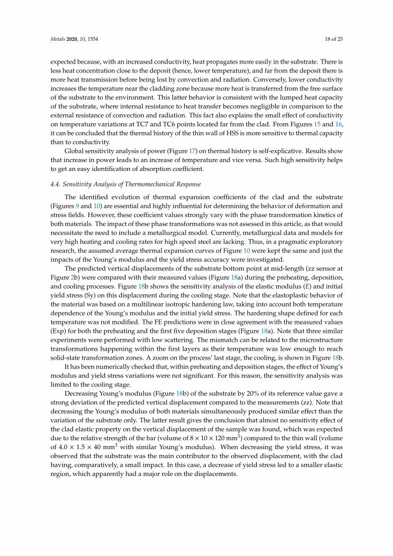
Metals 2020, 10, 1554 18 of 25

expected because, with an increased conductivity, heat propagates more easily in the substrate. There isless heat concentration close to the deposit (hence, lower temperature), and far from the deposit there ismore heat transmission before being lost by convection and radiation. Conversely, lower conductivityincreases the temperature near the cladding zone because more heat is transferred from the free surfaceof the substrate to the environment. This latter behavior is consistent with the lumped heat capacityof the substrate, where internal resistance to heat transfer becomes negligible in comparison to theexternal resistance of convection and radiation. This fact also explains the small effect of conductivityon temperature variations at TC7 and TC6 points located far from the clad. From Figures 15 and 16,it can be concluded that the thermal history of the thin wall of HSS is more sensitive to thermal capacitythan to conductivity.

Global sensitivity analysis of power (Figure 17) on thermal history is self-explicative. Results showthat increase in power leads to an increase of temperature and vice versa. Such high sensitivity helpsto get an easy identification of absorption coefficient.

4.4. Sensitivity Analysis of Thermomechanical Response

The identified evolution of thermal expansion coefficients of the clad and the substrate(Figures 9 and 10) are essential and highly influential for determining the behavior of deformation andstress fields. However, these coefficient values strongly vary with the phase transformation kinetics ofboth materials. The impact of these phase transformations was not assessed in this article, as that wouldnecessitate the need to include a metallurgical model. Currently, metallurgical data and models forvery high heating and cooling rates for high speed steel are lacking. Thus, in a pragmatic exploratoryresearch, the assumed average thermal expansion curves of Figure 10 were kept the same and just theimpacts of the Young’s modulus and the yield stress accuracy were investigated.

The predicted vertical displacements of the substrate bottom point at mid-length (zz sensor atFigure 2b) were compared with their measured values (Figure 18a) during the preheating, deposition,and cooling processes. Figure 18b shows the sensitivity analysis of the elastic modulus (E) and initialyield stress (Sy) on this displacement during the cooling stage. Note that the elastoplastic behavior ofthe material was based on a multilinear isotropic hardening law, taking into account both temperaturedependence of the Young’s modulus and the initial yield stress. The hardening shape defined for eachtemperature was not modified. The FE predictions were in close agreement with the measured values(Exp) for both the preheating and the first five deposition stages (Figure 18a). Note that three similarexperiments were performed with low scattering. The mismatch can be related to the microstructuretransformations happening within the first layers as their temperature was low enough to reachsolid-state transformation zones. A zoom on the process’ last stage, the cooling, is shown in Figure 18b.

It has been numerically checked that, within preheating and deposition stages, the effect of Young’smodulus and yield stress variations were not significant. For this reason, the sensitivity analysis waslimited to the cooling stage.

Decreasing Young’s modulus (Figure 18b) of the substrate by 20% of its reference value gave astrong deviation of the predicted vertical displacement compared to the measurements (zz). Note thatdecreasing the Young’s modulus of both materials simultaneously produced similar effect than thevariation of the substrate only. The latter result gives the conclusion that almost no sensitivity effect ofthe clad elastic property on the vertical displacement of the sample was found, which was expecteddue to the relative strength of the bar (volume of 8 × 10 × 120 mm3) compared to the thin wall (volumeof 4.0 × 1.5 × 40 mm3 with similar Young’s modulus). When decreasing the yield stress, it wasobserved that the substrate was the main contributor to the observed displacement, with the cladhaving, comparatively, a small impact. In this case, a decrease of yield stress led to a smaller elasticregion, which apparently had a major role on the displacements.

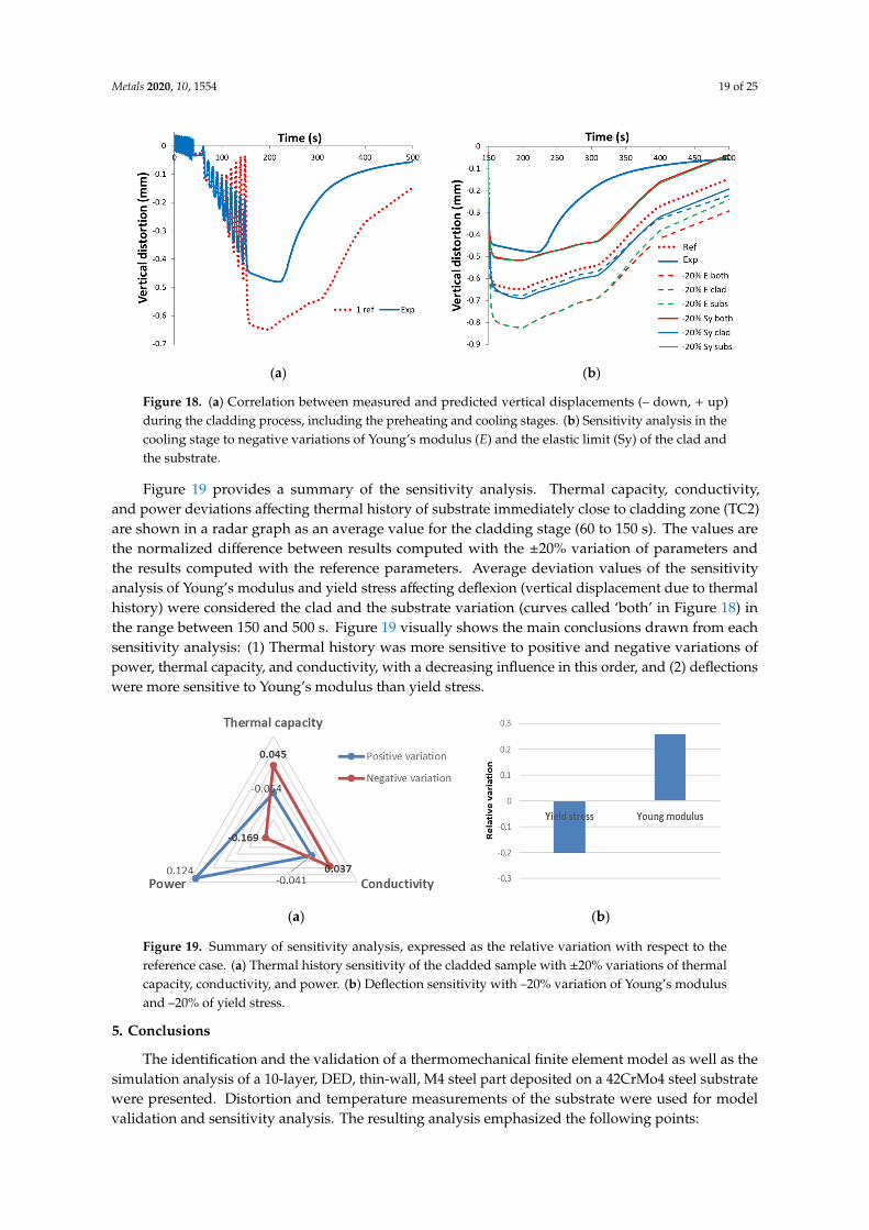
Metals 2020, 10, 1554 19 of 25

Metals 2020, 10, x FOR PEER REVIEW 18 of 24

The predicted vertical displacements of the substrate bottom point at mid-length (zz sensor at Figure 2b) were compared with their measured values (Figure 18a) during the preheating, deposition, and cooling processes. Figure 18b shows the sensitivity analysis of the elastic modulus (E) and initial yield stress (Sy) on this displacement during the cooling stage. Note that the elastoplastic behavior of the material was based on a multilinear isotropic hardening law, taking into account both temperature dependence of the Young’s modulus and the initial yield stress. The hardening shape defined for each temperature was not modified. The FE predictions were in close agreement with the measured values (Exp) for both the preheating and the first five deposition stages (Figure 18a). Note that three similar experiments were performed with low scattering. The mismatch can be related to the microstructure transformations happening within the first layers as their temperature was low enough to reach solid-state transformation zones. A zoom on the process’ last stage, the cooling, is shown in Figure 18b.

(a) (b)

Figure 18. (a) Correlation between measured and predicted vertical displacements (– down, + up) during the cladding process, including the preheating and cooling stages. (b) Sensitivity analysis in the cooling stage to negative variations of Young’s modulus (E) and the elastic limit (Sy) of the clad and the substrate.

It has been numerically checked that, within preheating and deposition stages, the effect of Young’s modulus and yield stress variations were not significant. For this reason, the sensitivity analysis was limited to the cooling stage.

Decreasing Young’s modulus (Figure 18b) of the substrate by 20% of its reference value gave a strong deviation of the predicted vertical displacement compared to the measurements (zz). Note that decreasing the Young’s modulus of both materials simultaneously produced similar effect than the variation of the substrate only. The latter result gives the conclusion that almost no sensitivity effect of the clad elastic property on the vertical displacement of the sample was found, which was expected due to the relative strength of the bar (volume of 8 × 10 × 120 mm3) compared to the thin wall (volume of 4.0 × 1.5 × 40 mm3 with similar Young’s modulus). When decreasing the yield stress, it was observed that the substrate was the main contributor to the observed displacement, with the clad having, comparatively, a small impact. In this case, a decrease of yield stress led to a smaller elastic region, which apparently had a major role on the displacements.

Figure 19 provides a summary of the sensitivity analysis. Thermal capacity, conductivity, and power deviations affecting thermal history of substrate immediately close to cladding zone (TC2) are shown in a radar graph as an average value for the cladding stage (60 to 150 s). The values are the normalized difference between results computed with the ±20% variation of parameters and the results computed with the reference parameters. Average deviation values of the sensitivity analysis of Young’s modulus and yield stress affecting deflexion (vertical displacement due to thermal history) were considered the clad and the substrate variation (curves called ‘both’ in Figure 18) in the range between 150 and 500 s. Figure 19 visually shows the main conclusions drawn from each

Figure 18. (a) Correlation between measured and predicted vertical displacements (– down, + up)during the cladding process, including the preheating and cooling stages. (b) Sensitivity analysis in thecooling stage to negative variations of Young’s modulus (E) and the elastic limit (Sy) of the clad andthe substrate.

Figure 19 provides a summary of the sensitivity analysis. Thermal capacity, conductivity,and power deviations affecting thermal history of substrate immediately close to cladding zone (TC2)are shown in a radar graph as an average value for the cladding stage (60 to 150 s). The values arethe normalized difference between results computed with the ±20% variation of parameters andthe results computed with the reference parameters. Average deviation values of the sensitivityanalysis of Young’s modulus and yield stress affecting deflexion (vertical displacement due to thermalhistory) were considered the clad and the substrate variation (curves called ‘both’ in Figure 18) inthe range between 150 and 500 s. Figure 19 visually shows the main conclusions drawn from eachsensitivity analysis: (1) Thermal history was more sensitive to positive and negative variations ofpower, thermal capacity, and conductivity, with a decreasing influence in this order, and (2) deflectionswere more sensitive to Young’s modulus than yield stress.

Metals 2020, 10, x FOR PEER REVIEW 19 of 24

sensitivity analysis: (1) Thermal history was more sensitive to positive and negative variations of power, thermal capacity, and conductivity, with a decreasing influence in this order, and (2) deflections were more sensitive to Young’s modulus than yield stress.

(a) (b)

Figure 19. Summary of sensitivity analysis, expressed as the relative variation with respect to the reference case. (a) Thermal history sensitivity of the cladded sample with ±20% variations of thermal capacity, conductivity, and power. (b) Deflection sensitivity with –20% variation of Young’s modulus and –20% of yield stress.

5. Conclusions

The identification and the validation of a thermomechanical finite element model as well as the simulation analysis of a 10-layer, DED, thin-wall, M4 steel part deposited on a 42CrMo4 steel substrate were presented. Distortion and temperature measurements of the substrate were used for model validation and sensitivity analysis. The resulting analysis emphasized the following points:

• Predicted thermal history can successfully explain SEM and OM observations of solidified microstructure showing variation from the first to the 10th layer of the thin wall;

• From the thermal point of view, the most influential factor was laser power, followed by thermal capacity and, finally, thermal conductivity; and

• Deflection of the substrate during the process was more sensitive to Young’s modulus than to yield stress.

M4 steel needs preheating in DED process and presents solid phase transformations (bainite, martensite) sensitive to temperature rate, as well as carbide formations that modify austenite composition and martensite temperature start (variation can be higher than 80 °C). The accurate thermomechanical cladding simulation of this material is still a challenge as accurate data on transformation kinetics and associated thermal dilatation curves are still missing as well as accurate thermal and phase dependent Young’s modulus.

Due to the multiple uncertainties, a deep learning approach is currently being investigated in addition to complementary material characterizations to improve the FE model and its set of material parameters. The final research goal is to determine the optimal process conditions that generate samples with low residual stresses and a homogeneous material. This last feature can be expected through a constant size of the melt pool for each clad layer.

Author Contributions: Simulations, validation, formal analysis, investigation, data curation, writing—original draft preparation, writing—review and editing, R.T.J. and A.M.H.; writing—review and editing, formal analysis, writing—original draft preparation V.T.; software developments, H.S.T.; project administration, A.M.H.; experiment, R.C.; analysis of experimental results and simulation assumptions, N.H., A.M., and J.T.; conceptualization and methodology, A.M.H. and L.D., thermophysical properties, N.H. All authors have read and agreed to the published version of the manuscript.

Funding: Funded by the FNRS F.R.S. [PDR T.0039.14] Grant, Laser cladding.

Figure 19. Summary of sensitivity analysis, expressed as the relative variation with respect to thereference case. (a) Thermal history sensitivity of the cladded sample with ±20% variations of thermalcapacity, conductivity, and power. (b) Deflection sensitivity with –20% variation of Young’s modulusand –20% of yield stress.

5. Conclusions

The identification and the validation of a thermomechanical finite element model as well as thesimulation analysis of a 10-layer, DED, thin-wall, M4 steel part deposited on a 42CrMo4 steel substratewere presented. Distortion and temperature measurements of the substrate were used for modelvalidation and sensitivity analysis. The resulting analysis emphasized the following points:

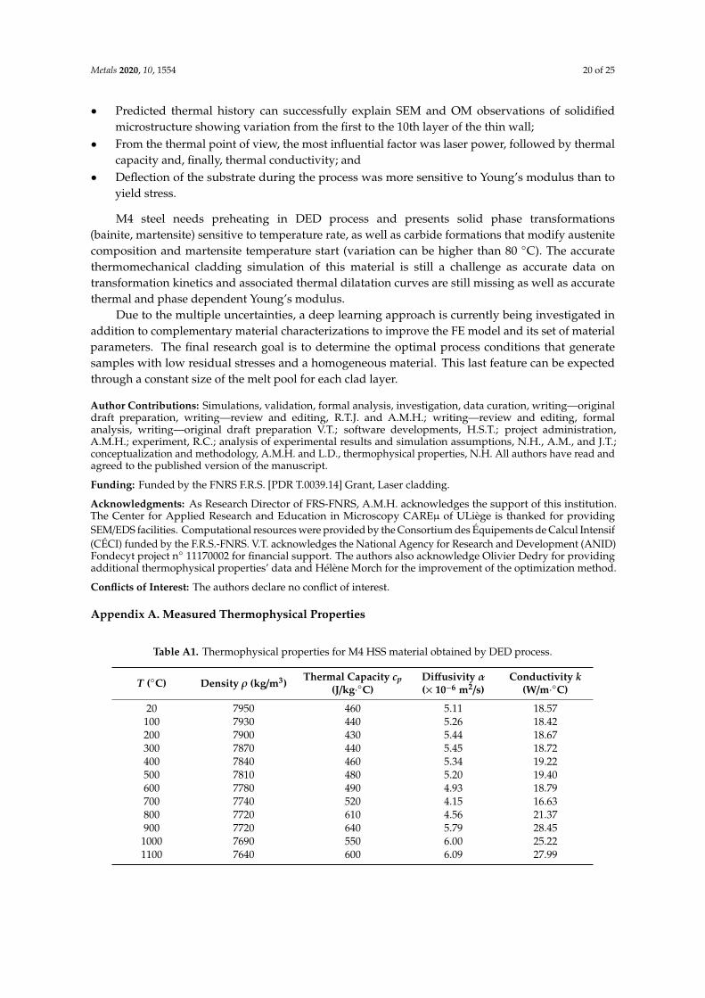
Metals 2020, 10, 1554 20 of 25

• Predicted thermal history can successfully explain SEM and OM observations of solidifiedmicrostructure showing variation from the first to the 10th layer of the thin wall;

• From the thermal point of view, the most influential factor was laser power, followed by thermalcapacity and, finally, thermal conductivity; and

• Deflection of the substrate during the process was more sensitive to Young’s modulus than toyield stress.

M4 steel needs preheating in DED process and presents solid phase transformations(bainite, martensite) sensitive to temperature rate, as well as carbide formations that modify austenitecomposition and martensite temperature start (variation can be higher than 80 ◦C). The accuratethermomechanical cladding simulation of this material is still a challenge as accurate data ontransformation kinetics and associated thermal dilatation curves are still missing as well as accuratethermal and phase dependent Young’s modulus.

Due to the multiple uncertainties, a deep learning approach is currently being investigated inaddition to complementary material characterizations to improve the FE model and its set of materialparameters. The final research goal is to determine the optimal process conditions that generatesamples with low residual stresses and a homogeneous material. This last feature can be expectedthrough a constant size of the melt pool for each clad layer.

Author Contributions: Simulations, validation, formal analysis, investigation, data curation, writing—originaldraft preparation, writing—review and editing, R.T.J. and A.M.H.; writing—review and editing, formalanalysis, writing—original draft preparation V.T.; software developments, H.S.T.; project administration,A.M.H.; experiment, R.C.; analysis of experimental results and simulation assumptions, N.H., A.M., and J.T.;conceptualization and methodology, A.M.H. and L.D., thermophysical properties, N.H. All authors have read andagreed to the published version of the manuscript.

Funding: Funded by the FNRS F.R.S. [PDR T.0039.14] Grant, Laser cladding.

Acknowledgments: As Research Director of FRS-FNRS, A.M.H. acknowledges the support of this institution.The Center for Applied Research and Education in Microscopy CAREµ of ULiège is thanked for providingSEM/EDS facilities. Computational resources were provided by the Consortium des Équipements de Calcul Intensif(CÉCI) funded by the F.R.S.-FNRS. V.T. acknowledges the National Agency for Research and Development (ANID)Fondecyt project n◦ 11170002 for financial support. The authors also acknowledge Olivier Dedry for providingadditional thermophysical properties’ data and Hélène Morch for the improvement of the optimization method.

Conflicts of Interest: The authors declare no conflict of interest.

Appendix A. Measured Thermophysical Properties

Table A1. Thermophysical properties for M4 HSS material obtained by DED process.

T (◦C) Density ρ (kg/m3)Thermal Capacity cp

(J/kg·◦C)Diffusivity α(× 10−6 m2/s)

Conductivity k(W/m·◦C)

20 7950 460 5.11 18.57100 7930 440 5.26 18.42200 7900 430 5.44 18.67300 7870 440 5.45 18.72400 7840 460 5.34 19.22500 7810 480 5.20 19.40600 7780 490 4.93 18.79700 7740 520 4.15 16.63800 7720 610 4.56 21.37900 7720 640 5.79 28.45

1000 7690 550 6.00 25.221100 7640 600 6.09 27.99

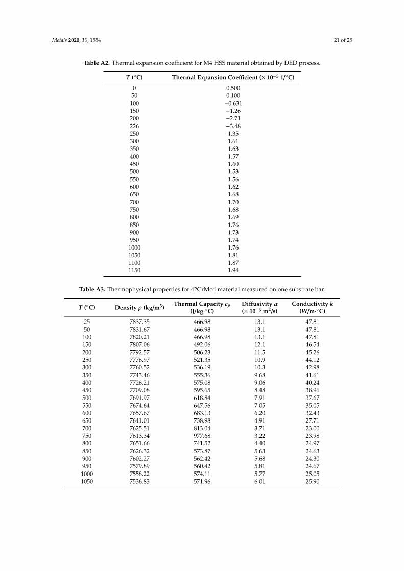
Metals 2020, 10, 1554 21 of 25

Table A2. Thermal expansion coefficient for M4 HSS material obtained by DED process.

T (◦C) Thermal Expansion Coefficient (× 10−5 1/◦C)

0 0.50050 0.100100 −0.631150 −1.26200 −2.71226 −3.48250 1.35300 1.61350 1.63400 1.57450 1.60500 1.53550 1.56600 1.62650 1.68700 1.70750 1.68800 1.69850 1.76900 1.73950 1.74

1000 1.761050 1.811100 1.871150 1.94

Table A3. Thermophysical properties for 42CrMo4 material measured on one substrate bar.

T (◦C) Density ρ (kg/m3)Thermal Capacity cp

(J/kg·◦C)Diffusivity α(× 10−6 m2/s)

Conductivity k(W/m·◦C)

25 7837.35 466.98 13.1 47.8150 7831.67 466.98 13.1 47.81

100 7820.21 466.98 13.1 47.81150 7807.06 492.06 12.1 46.54200 7792.57 506.23 11.5 45.26250 7776.97 521.35 10.9 44.12300 7760.52 536.19 10.3 42.98350 7743.46 555.36 9.68 41.61400 7726.21 575.08 9.06 40.24450 7709.08 595.65 8.48 38.96500 7691.97 618.84 7.91 37.67550 7674.64 647.56 7.05 35.05600 7657.67 683.13 6.20 32.43650 7641.01 738.98 4.91 27.71700 7625.51 813.04 3.71 23.00750 7613.34 977.68 3.22 23.98800 7651.66 741.52 4.40 24.97850 7626.32 573.87 5.63 24.63900 7602.27 562.42 5.68 24.30950 7579.89 560.42 5.81 24.67

1000 7558.22 574.11 5.77 25.051050 7536.83 571.96 6.01 25.90

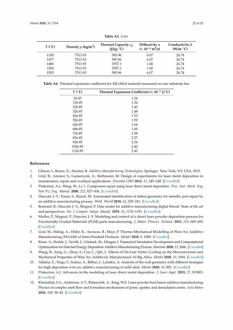
Metals 2020, 10, 1554 22 of 25

Table A3. Cont.

T (◦C) Density ρ (kg/m3)Thermal Capacity cp

(J/kg·◦C)Diffusivity α(× 10−6 m2/s)

Conductivity k(W/m·◦C)

1100 7513.93 585.96 6.07 26.741477 7513.93 585.96 6.07 26.741480 7513.93 3557.1 1.00 26.741500 7513.93 3557.1 1.00 26.741503 7513.93 585.96 6.07 26.74

Table A4. Thermal expansion coefficient for 42CrMo4 material measured on one substrate bar.

T (◦C) Thermal Expansion Coefficient (× 10−5 1/◦C)

26.85 1.24126.85 1.34226.85 1.43326.85 1.48426.85 1.53526.85 1.59626.85 1.64686.85 1.00726.85 1.58826.85 2.27926.85 2.34

1026.85 2.401126.85 2.42

References

1. Gibson, I.; Rosen, D.; Stucker, B. Additive Manufacturing Technologies; Springer: New York, NY, USA, 2015.2. Graf, B.; Ammer, S.; Gumenyuk, A.; Rethmeier, M. Design of experiments for laser metal deposition in

maintenance, repair and overhaul applications. Procedia CIRP 2013, 11, 245–248. [CrossRef]3. Pinkerton, A.J.; Wang, W.; Li, L. Component repair using laser direct metal deposition. Proc. Inst. Mech. Eng.

Part B J. Eng. Manuf. 2008, 222, 827–836. [CrossRef]4. Hascoët, J.-Y.; Touzé, S.; Rauch, M. Automated identification of defect geometry for metallic part repair by

an additive manufacturing process. Weld. World 2018, 62, 229–241. [CrossRef]5. Bonnard, R.; Hascoët, J.-Y.; Mognol, P. Data model for additive manufacturing digital thread: State of the art

and perspectives. Int. J. Comput. Integr. Manuf. 2019, 32, 1170–1191. [CrossRef]6. Muller, P.; Mognol, P.; Hascoet, J.-Y. Modeling and control of a direct laser powder deposition process for

Functionally Graded Materials (FGM) parts manufacturing. J. Mater. Process. Technol. 2013, 213, 685–692.[CrossRef]

7. Graf, M.; Hälsig, A.; Höfer, K.; Awiszus, B.; Mayr, P. Thermo-Mechanical Modelling of Wire-Arc AdditiveManufacturing (WAAM) of Semi-Finished Products. Metals 2018, 8, 1009. [CrossRef]

8. Kiran, A.; Hodek, J.; Vavrík, J.; Urbánek, M.; Džugan, J. Numerical Simulation Development and ComputationalOptimization for Directed Energy Deposition Additive Manufacturing Process. Materials 2020, 13, 2666. [CrossRef]

9. Wang, B.; Yang, G.; Zhou, S.; Cui, C.; Qin, L. Effects of On-Line Vortex Cooling on the Microstructure andMechanical Properties of Wire Arc Additively Manufactured Al-Mg Alloy. Metals 2020, 10, 1004. [CrossRef]

10. Aldalur, E.; Veiga, F.; Suárez, A.; Bilbao, J.; Lamikiz, A. Analysis of the wall geometry with different strategiesfor high deposition wire arc additive manufacturing of mild steel. Metals 2020, 10, 892. [CrossRef]

11. Pinkerton, A.J. Advances in the modeling of laser direct metal deposition. J. Laser Appl. 2015, 27, S15001.[CrossRef]

12. Khairallah, S.A.; Anderson, A.T.; Rubenchik, A.; King, W.E. Laser powder-bed fusion additive manufacturing:Physics of complex melt flow and formation mechanisms of pores, spatter, and denudation zones. Acta Mater.2016, 108, 36–45. [CrossRef]

Metals 2020, 10, 1554 23 of 25

13. Heeling, T.; Cloots, M.; Wegener, K. Melt pool simulation for the evaluation of process parameters in selectivelaser melting. Addit. Manuf. 2017, 14, 116–125. [CrossRef]

14. Pinomaa, T.; Provatas, N. Quantitative phase field modeling of solute trapping and continuous growthkinetics in quasi-rapid solidification. Acta Mater. 2019, 168, 167–177. [CrossRef]

15. Touzé, S. Laser Metal Deposition of Aluminum-Copper Alloys for Repair Applications. Ph.D. Thesis,École Centrale de Nantes, Nantes, France, 15 September 2019.

16. Jardin, R.T.; Tchuindjang, J.T.; Duchêne, L.; Tran, H.-S.; Hashemi, N.; Carrus, R.; Mertens, A.; Habraken, A.M.Thermal histories and microstructures in Direct Energy Deposition of a High Speed Steel thick deposit.Mater. Lett. 2019, 236, 42–45. [CrossRef]

17. Delahaye, J.; Tchuindjang, J.T.; Lecomte-Beckers, J.; Rigo, O.; Habraken, A.M.; Mertens, A. Influence of Siprecipitates on fracture mechanisms of AlSi10Mg parts processed by Selective Laser Melting. Acta Mater.2019, 175, 160–170. [CrossRef]

18. Setien, I.; Chiumenti, M.; van der Veen, S.; San Sebastian, M.; Garciandía, F.; Echeverría, A. Empiricalmethodology to determine inherent strains in additive manufacturing. Comput. Math. Appl. 2019, 78,2282–2295. [CrossRef]

19. Yang, Q.; Zhang, P.; Cheng, L.; Min, Z.; Chyu, M.; To, A.C. Finite element modeling and validation ofthermomechanical behavior of Ti-6Al-4V in directed energy deposition additive manufacturing. Addit. Manuf.2016, 12, 169–177. [CrossRef]

20. Patil, R.B.; Yadava, V. Finite element analysis of temperature distribution in single metallic powder layerduring metal laser sintering. Int. J. Mach. Tools Manuf. 2007, 47, 1069–1080. [CrossRef]

21. Yin, J.; Zhu, H.; Ke, L.; Lei, W.; Dai, C.; Zuo, D. Simulation of temperature distribution in single metallicpowder layer for laser micro-sintering. Comput. Mater. Sci. 2012, 53, 333–339. [CrossRef]

22. Chiumenti, M.; Lin, X.; Cervera, M.; Lei, W.; Zheng, Y.; Huang, W. Numerical simulation and experimentalcalibration of additive manufacturing by blown powder technology. Part I: Thermal analysis. Rapid Prototyp. J.2017, 23, 448–463. [CrossRef]

23. Ye, R.; Smugeresky, J.E.; Zheng, B.; Zhou, Y.; Lavernia, E.J. Numerical modeling of the thermal behaviorduring the LENS®process. Mater. Sci. Eng. A 2006, 428, 47–53. [CrossRef]

24. He, X.; Yu, G.; Mazumder, J. Temperature and composition profile during double-track laser cladding of H13tool steel. J. Phys. D Appl. Phys. 2010, 43, 015502. [CrossRef]

25. Heigel, J.C.; Michaleris, P.; Reutzel, E.W. Thermo-mechanical model development and validation of directedenergy deposition additive manufacturing of Ti–6Al–4V. Addit. Manuf. 2015, 5, 9–19. [CrossRef]

26. Goldak, J.; Chakravarti, A.; Bibby, M. A new finite element model for welding heat sources. Metall. Trans. B1984, 15, 299–305. [CrossRef]

27. Yang, J.; Sun, S.; Brandt, M.; Yan, W. Experimental investigation and 3D finite element prediction of theheat affected zone during laser assisted machining of Ti6Al4V alloy. J. Mater. Process. Technol. 2010, 210,2215–2222. [CrossRef]

28. Tran, H.-S.; Tchuindjang, J.T.; Paydas, H.; Mertens, A.; Jardin, R.T.; Duchêne, L.; Carrus, R.; Lecomte-Beckers, J.;Habraken, A.M. 3D thermal finite element analysis of laser cladding processed Ti-6Al-4V part withmicrostructural correlations. Mater. Des. 2017, 128, 130–142. [CrossRef]

29. Lindgren, L.-E.; Lundbäck, A.; Fisk, M.; Pederson, R.; Andersson, J. Simulation of additive manufacturingusing coupled constitutive and microstructure models. Addit. Manuf. 2016, 12, 144–158. [CrossRef]

30. Caiazzo, F.; Alfieri, V. Simulation of Laser-assisted Directed Energy Deposition of Aluminum Powder:Prediction of Geometry and Temperature Evolution. Materials 2019, 12, 2100. [CrossRef]

31. Lu, X.; Lin, X.; Chiumenti, M.; Cervera, M.; Li, J.; Ma, L.; Wei, L.; Hu, Y.; Huang, W. Finite element analysis andexperimental validation of the thermomechanical behavior in laser solid forming of Ti-6Al-4V. Addit. Manuf.2018, 21, 30–40. [CrossRef]

32. Shim, D.-S.; Baek, G.-Y.; Lee, E.-M. Effect of substrate preheating by induction heater on direct energydeposition of AISI M4 powder. Mater. Sci. Eng. A 2017, 682, 550–562. [CrossRef]

33. Hashemi, N.; Mertens, A.; Montrieux, H.-M.; Tchuindjang, J.T.; Dedry, O.; Carrus, R.; Lecomte-Beckers, J.Oxidative wear behaviour of laser clad High Speed Steel thick deposits: Influence of sliding speed, carbidetype and morphology. Surf. Coat. Technol. 2017, 315, 519–529. [CrossRef]

Metals 2020, 10, 1554 24 of 25

34. Pineda Huitron, R.M.; Ramirez Lopez, P.E.; Vuorinen, E.; Jentner, R.; Kärkkäinen, M.E. Converging criteria tocharacterize crack susceptibility in a micro-alloyed steel during continuous casting. Mater. Sci. Eng. A 2020,772, 138691. [CrossRef]

35. Wang, S.-H.; Chen, J.-Y.; Xue, L. A study of the abrasive wear behaviour of laser-clad tool steel coatings.Surf. Coat. Technol. 2006, 200, 3446–3458. [CrossRef]

36. Leunda, J.; Soriano, C.; Sanz, C.; Navas, V.G. Laser Cladding of Vanadium-Carbide Tool Steels for Die Repair.Phys. Procedia 2011, 12, 345–352. [CrossRef]

37. Rahman, N.U.; Capuano, L.; Cabeza, S.; Feinaeugle, M.; Garcia-Junceda, A.; de Rooij, M.B.; Matthews, D.T.A.;Walmag, G.; Gibson, I.; Römer, G.R.B.E. Directed energy deposition and characterization of high-carbon highspeed steels. Addit. Manuf. 2019, 30, 100838. [CrossRef]

38. Pascon, F.; Cescotto, S.; Habraken, A.M. A 2.5D finite element model for bending and straightening incontinuous casting of steel slabs. Int. J. Numer. Methods Eng. 2006, 68, 125–149. [CrossRef]

39. Neira Torres, I.; Gilles, G.; Tchuindjang, J.T.; Flores, P.; Lecomte-Beckers, J.; Habraken, A.M. FE modelingof the cooling and tempering steps of bimetallic rolling mill rolls. Int. J. Mater. Form. 2017, 10, 287–305.[CrossRef]

40. Guzmán, C.F.; Gu, J.; Duflou, J.; Vanhove, H.; Flores, P.; Habraken, A.M. Study of the geometrical inaccuracyon a SPIF two-slope pyramid by finite element simulations. Int. J. Solids Struct. 2012, 49, 3594–3604.[CrossRef]

41. Mukherjee, T.; Zhang, W.; DebRoy, T. An improved prediction of residual stresses and distortion in additivemanufacturing. Comput. Mater. Sci. 2017, 126, 360–372. [CrossRef]

42. Chew, Y.; Pang, J.H.L.; Bi, G.; Song, B. Thermo-mechanical model for simulating laser cladding inducedresidual stresses with single and multiple clad beads. J. Mater. Process. Technol. 2015, 224, 89–101. [CrossRef]

43. Zhu, Y.Y.; Cescotto, S. Unified and mixed formulation of the 8-node hexahedral elements by assumed strainmethod. Comput. Methods Appl. Mech. Eng. 1996, 129, 177–209. [CrossRef]

44. Belytschko, T.; Bindeman, L.P. Assumed strain stabilization of the 4-node quadrilateral with 1-pointquadrature for nonlinear problems. Comput. Methods Appl. Mech. Eng. 1991, 88, 311–340. [CrossRef]

45. Duchêne, L.; El Houdaigui, F.; Habraken, A.M. Length changes and texture prediction during free endtorsion test of copper bars with FEM and remeshing techniques. Int. J. Plast. 2007, 23, 1417–1438. [CrossRef]

46. Simo, J.C.; Hughes, T.J.R. On the Variational Foundations of Assumed Strain Methods. J. Appl. Mech. 1986,53, 51–54. [CrossRef]

47. Cao, J.; Gharghouri, M.A.; Nash, P. Finite-element analysis and experimental validation of thermal residualstress and distortion in electron beam additive manufactured Ti-6Al-4V build plates. J. Mater. Process. Technol.2016, 237, 409–419. [CrossRef]

48. Bi, G.; Gasser, A.; Wissenbach, K.; Drenker, A.; Poprawe, R. Identification and qualification of temperaturesignal for monitoring and control in laser cladding. Opt. Lasers Eng. 2006, 44, 1348–1359. [CrossRef]

49. Lampa, C.; Kaplan, A.F.H.; Powell, J.; Magnusson, C. An analytical thermodynamic model of laser welding.J. Phys. D Appl. Phys. 1997, 30, 1293–1299. [CrossRef]

50. Neela, V.; De, A. Three-dimensional heat transfer analysis of LENSTM process using finite element method.Int. J. Adv. Manuf. Technol. 2009, 45, 935–943. [CrossRef]

51. Deng, D.; Kiyoshima, S. FEM prediction of welding residual stresses in a SUS304 girth-welded pipe withemphasis on stress distribution near weld start/end location. Comput. Mater. Sci. 2010, 50, 612–621. [CrossRef]

52. Liang, W.; Murakawa, H.; Deng, D. Investigation of welding residual stress distribution in a thick-plate jointwith an emphasis on the features near weld end-start. Mater. Des. 2015, 67, 303–312. [CrossRef]

53. Denlinger, E.R.; Michaleris, P. Effect of stress relaxation on distortion in additive manufacturing processmodeling. Addit. Manuf. 2016, 12, 51–59. [CrossRef]

54. Lu, X.; Lin, X.; Chiumenti, M.; Cervera, M.; Hu, Y.; Ji, X.; Ma, L.; Huang, W. In situ measurements andthermo-mechanical simulation of Ti–6Al–4V laser solid forming processes. Int. J. Mech. Sci. 2019, 153–154,119–130. [CrossRef]

55. Lu, X.; Lin, X.; Chiumenti, M.; Cervera, M.; Hu, Y.; Ji, X.; Ma, L.; Yang, H.; Huang, W. Residual stress anddistortion of rectangular and S-shaped Ti-6Al-4V parts by Directed Energy Deposition: Modelling andexperimental calibration. Addit. Manuf. 2019, 26, 166–179. [CrossRef]

56. CTSPM. M4 PM Catalogue; Cincinnati Tool Steel Company Inc.: Rockford, IL, USA, 2020. Available online:http://cintool.com/documents/Powdered_Metal/M4PM.pdf (accessed on 9 June 2020).

Metals 2020, 10, 1554 25 of 25

57. Jiangyou. Data Table for GS-42CrMo4; Jiangyou Longhai Special Steel Co.: Jiangyou, China, 2020. Available online:http://www.steelgr.com/Steel-Grades/Mould-Steel/gs-42crmo4.html (accessed on 9 June 2020).

58. ABRAMS. Technical Guide: AFNOR 42CD4; Abrams Engineering Services GmbH & Co. KG: Osnabrück,Germany, 2020. Available online: http://www.aciers-premium.fr/images/filedownloads/fichestechniques/42CD4.pdfml (accessed on 9 June 2020).

59. Tuninetti, V.; Flores, P.; Valenzuela, M.; Pincheira, G.; Medina, C.; Duchêne, L.; Habraken, A.-M. Experimentalcharacterization of the compressive mechanical behaviour of Ti6Al4V alloy at constant strain rates over thefull elastoplastic range. Int. J. Mater. Form. 2020, 13, 709–724. [CrossRef]

60. Habraken, A.M.; Bouffioux, C. Simulation des Changements de Phases Lors de la Trempe d’un AnneauAnalyse Thermique, Mécanique, Métallurgique CFR—Acier 42CD4; Technical Report 57 Region WalloonProject—Caractérisation Rationnelle des Propriétés à Chaud des Matériaux Métalliques; Convention N◦

981/3793; MSM, University of Liège: Liège, Belgium, 2003.61. Hashemi, N. Study of High Speed Steel Deposits Produced by Laser Cladding, Microstructure—Wear—Thermal

Model. Ph.D. Thesis, University of Liège, Liège, Belgium, 8 September 2017.

Publisher’s Note: MDPI stays neutral with regard to jurisdictional claims in published maps and institutionalaffiliations.

© 2020 by the authors. Licensee MDPI, Basel, Switzerland. This article is an open accessarticle distributed under the terms and conditions of the Creative Commons Attribution(CC BY) license (http://creativecommons.org/licenses/by/4.0/).