Steam De Pleijt-Nuvolari-Weisdorf 28 November 2016 · PDF fileFernihough, Oded Galor, Alexander Field, Ralf Meisenzahl, Jaime ... Jan Luiten van Zanden, and Nico Voigtlander for help

Human Capital Formation during the First Industrial Revolution:

Evidence from the Use of Steam Engines§

Alexandra M. de Pleijt London School of Economics and Utrecht University

Alessandro Nuvolari Sant’ Anna School of Advanced Studies

Jacob Weisdorf University of Southern Denmark and CEPR

Abstract We examine the effect of technological change on human capital formation during England’s Industrial Revolution. Using the number of steam engines installed by 1800 to capture technological change and occupational statistics to measure working skills (using HISCLASS), our county-level regression analysis shows a negative correlation between the use of steam engines and the share of unskilled workers. We use exogenous variation in carboniferous rock strata (containing coal to fuel the engines) to show that the effect was causal. Technological change had, however, no significant effect on basic educational training including literacy and school enrollment rates. Keywords: Economic Growth, Education, Human Capital, Industrialisation, Technological Progress, Steam Engines JEL codes: J82, N33, O14, O33

§ We thank the seminar and conference audience at the 16th World Economic History Conference, the CAGE/HEDG Workshop on Economic Geography and History, the 2016 Economic History Association, Rutgers University, Utrecht University, and the London School of Economics for helpful comments and suggestions. We are grateful to Leigh Shaw-Taylor for sharing the occupational data of the Cambridge Group; to Helen Aitchison for proof reading; and to Sascha Becker, Dan Bogart, Michael Bordo, Greg Clark, Alan Fernihough, Oded Galor, Alexander Field, Ralf Meisenzahl, Jaime Reis, Natacha Postel-Vinay, Eric Schneider, Jan Luiten van Zanden, and Nico Voigtlander for help with data preparation and various suggestions.

2

1. Introduction

Was technological progress during the Industrial Revolution skill-demanding or skill-saving?

Recent contributions in economic growh theory have argued for a positive effect of technical

change on human capital formation during the transition towards ‘modern economic growth’

(e.g. Galor 2011). This notion has recently received empirical support from 19th-centry

France (Franck and Galor 2016). Interestingly, the French evidence contrasts with the

traditional narrative about the effects of early industrialisation in England, where earlier work

have argued that skill-displacement was the main outcome of technological change. In

particular, the classical years of England’s Industrial Revolution were characterized by

stagnant rates of male literacy (e.g. Schofield 1973; Nicholas and Nicholas 1992; Mitch

1999); a decline in the average years of secondary schooling (de Pleijt 2015); a growth in the

share of unskilled workers (de Pleijt and Weisdorf 2017); and the absence of any increase of

the skill premium (e.g. Clark 2005; Van Zanden 2009; Allen 2009). Combined with a long list

of chronicles about machine-breaking riots, allegedly triggered by the workers’ fears that

industrialisation would render their skills redundant (Nuvolari 2002), the English case, at least

prima facie, seems to provide support to the Goldin and Katz (1998) hypothesis that the shift

from workshop to factory production reduced the need for skilled workers. But the effect of

new technology on human capital formation during England’s early Industrial Revolution has

not been tested formally.

This study breaks new ground along three lines. First, previous work attempting to

quantify the evolution of human capital in England during the Industrial Revolution has

mainly focused on literacy and numeracy rates. However, though meticulously documented

(Nicholas and Nicholas 1992; Mitch 1999; Baten et al. 2014), literacy and numeracy skills

measure only very basic competencies. For example, the literacy rate assigns the same level

of ability to a literate factory worker and a literate industrial engineer, with no distinction

3

being made between the large variations in aptitude required for these two very different

occupations. Moreover, the fact that any literacy and numeracy skills obtained were not

necessarily used productively, such as a factory worker’s ability to read and write, makes the

potential discrepancy between the acquisition of skills and the application of skills in

productive activities a relevant matter and one which is difficult to address using basic

competencies, such as literacy or numeracy, to measure human capital attainments.

In this study, thanks to early 19th-century occupational statistics provided by the

Cambridge Group for the History of Population and Social Structure and documented in

Shaw-Taylor et al (2012), we are able to classify over 2.6 million English male workers

according to the skill-content of their work. This categorisation of occupational titles by skill,

which is done by employing a standardised work-classification system (HISCO-HISCLASS),

allows us to quantify the shares of unskilled, lower-skilled, medium-skilled, and highly-

skilled workers by county and to explore the correlation between those shares and country-

specific technological change. The occupational data also enable us to identify the so-called

‘density in the upper tail of professional knowledge’ and to examine whether or not the

diffusion of new technology during the Industrial Revolution created a growing class of

highly-skilled mechanical workers, as proposed in recent studies (e.g. Mokyr 2005; Mokyr

and Voth 2009; Meisenzahl and Mokyr 2012; Squicciarini and Voigtländer 2015; Feldman

and van der Beek 2016). In addition to working skills derived from occupations, we also

make use of the more conventional indicators of human capital, including literacy rates and

school enrolment rates.

Second, we employ a methodological approch proposed in Franck and Galor (2016)

for historical France, taking it across the channel to England, the cradle of the Industrial

Revolution and the frontrunner in modern economic growth. Franck and Galor used regional

variation in the diffusion of steam technology to show that more steam engines were

4

associated with higher rates of literacy, more apprentices, more teachers, and more

schools. Similar to Franck and Galor, we exploit county-level variation in the use of steam

engines to investigate the effect of technological change on the process of human capital

formation in the English case. Our steam dataset is an updated version, previously used in

Nuvolari et al (2011), of that originally constructed by Kanefsky and Robey (1980).

Containing detailed information about all known steam engines built and installed in England,

from when the first steam engine prototype was patented by Thomas Savery, in 1698, up until

1800, this dataset represents the best quantitative appraisal of the early diffusion of steam

power during England’s Industrial Revolution (Nuvolari et al 2011).

Last but not least and in order to establish whether or not any observed effects were

causal, we use exogenous county-level variation in the prevalence of carboniferous rock strata

(Asch 2005) as an instrument for the number of steam engines. Because steam engines were

run on coal, which is found in the carboniferous rock strata, we are able to exploit the fact that

the share of a county’s carboniferous rock strata is highly correlated with the number of steam

engines installed by 1800, but that the prevalence of carboniferous rock is independent of our

pre-steam indicators of human capital formation.

Our empirical analysis shows that steam technology was positively associated with

working skills. More steam engines were linked to lower shares of unskilled workers

and higher shares of lower- and medium-skilled workers. We also establish that more engines

were connected with higher shares of highly-skilled mechanical workers, including engineers,

various wrights, machine makers and instrument makers, representing the ‘density in the

upper tail of professional knowledge’. However, our analysis documents that the use of steam

technology was either negatively associated with elementary education or had no significant

effect hereon. That is, more steam engines were linked to fewer primary schools per person

and lower school enrolment rates. Also, although more steam engines were not significantly

5

associated with literacy rates, we observe that counties with comparatively many steam

engines had comparatively higher gender inequality in literacy.

Using the prevalence of carboniferous rock strata as an instrument for the number of

steam engines, we document that a one standard-deviation increase in the number of steam

engines led to a 0.78 standard-deviation decrease in the share of unskilled workers. An

equally large effect of the implementation of early steam technology concerned the demand

for highly-skilled mechanical workmen, where we find that a one standard-deviation increase

in the number of steam engines caused a 0.91 standard-deviation increase in the share of

highly-skilled mechanical workers. We do not find any significant causal effects of steam

engines on elementary schooling, except for a positive effect of steam on gender inequality in

literacy. In particular, a one standard-deviation increase in the use of steam engines caused a

0.79 standard-deviation increase in gender inequality. Our findings are robust to accounting

for a wide range of confounding factors, including county-level geographical characteristics

and pre-industrial development performances, as well as the use of alternative mechanical

powers, including cotton-, wool-, and water-mills.

The ambiguous effect of the Industrial Revolution on the demand for skills supports

the pre-existing narrative that England’s early industrialisation either harmed or had a neutral

effect on elementary education (e.g. Nicholas and Nicholas 1992; Mitch 1999; de Pleijt 2015).

At the same time, the observed effects show that early industry positively influenced the

formation of formal working skills, particularly industry-specific ones, as pointed out in

previous studies (e.g., Mokyr 2005; Mokyr and Voth 2009; Van Der Beek 2012; Feldman and

van der Beek 2016). The observed results are in line with one of the key tenets of Unified

Growth Theory, according to which technological progress during the Industrial Revolution

prompted the creation of working skills (Galor and Weil 2000; Galor 2011). The ambiguous

6

nature of the findings also chime with theoretical work by O’Rourke et al (2013), arguing that

early technological progress could be skill-saving and skill-demanding at the same time.

The remainder of our paper is organised as follows. Section 2 presents the steam

engine data and the various indicators of human capital, as well as the confounding variables.

Section 3 explains the identification strategy and presents the results of our baseline OLS and

IV regressions. Section 4 demonstrates that the results are robust to introducing a wide range

of confounding factors. Section 5 summarises the main findings.

2. Data

We use cross-county variation in the number of steam engines built and installed by 1800 as a

proxy for industrial technological progress.1 The data used is an updated version of the steam

dataset originally constructed and published by Kanefsky and Robey (1980). The first steam

engine included in the dataset is the famous so-called atmospheric engine, which was

patented by Thomas Savery in 1698 and put to use in 1702 (Nuvolari et al 2011). During the

second half of the eighteenth century, steam engines were increasingly employed, especially

in the more innovative and dynamic branches of the English economy. By 1800 a total of

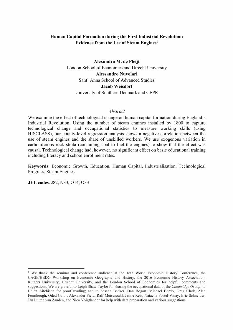
2,207 steam engines had been built and installed in England.

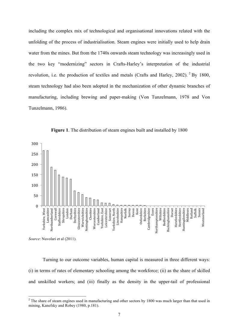
The intensity in the use of steam power varied considerably across the English

counties, as shown in Figure 1. Not surprisingly, steam engines were very common in

England’s industrial centres, including Lancashire and West Yorkshire, each of which had

over 250 engines installed by 1800. On the other hand, counties that were dominated by

agriculture during the classical years of the industrial revolution, such as Dorset and Sussex,

had no steam engines installed at all. Our basic assumption is that the intensity in steam

power adoption at county level can be taken as a synthetic indicator of technical change,

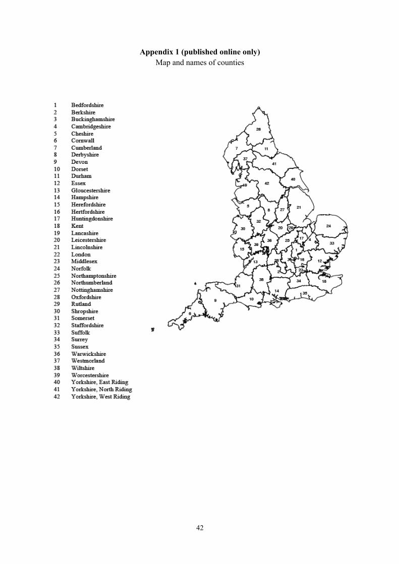
1 A map illustrating the location of the counties can be found in Appendix 1.

7

including the complex mix of technological and organisational innovations related with the

unfolding of the process of industrialisation. Steam engines were initially used to help drain

water from the mines. But from the 1740s onwards steam technology was increasingly used in

the two key “modernizing” sectors in Crafts-Harley’s interpretation of the industrial

revolution, i.e. the production of textiles and metals (Crafts and Harley, 2002). 2 By 1800,

steam technology had also been adopted in the mechanization of other dynamic branches of

manufacturing, including brewing and paper-making (Von Tunzelmann, 1978 and Von

Tunzelmann, 1986).

Figure 1. The distribution of steam engines built and installed by 1800

Source: Nuvolari et al (2011).

Turning to our outcome variables, human capital is measured in three different ways:

(i) in terms of rates of elementary schooling among the workforce; (ii) as the share of skilled

and unskilled workers; and (iii) finally as the density in the upper-tail of professional

2 The share of steam engines used in manufacturing and other sectors by 1800 was much larger than that used in mining, Kanefsky and Robey (1980, p.181).

0

50

100

150

200

250

300

Yorkshire, West

Lancashire

Northum

berland

Cornwall

Staffordshire

Shropshire

London

Durham

Derbyshire

Gloucestershire

Warwickshire

Nottingham

shire

Cheshire

Worcestershire

Cumberland

Yorkshire, East

Leicestershire

Somerset

Yorkshire, North

Lincolnshire

Ham

pshire

Norfolk

Surrey

Devon

Kent

Oxfordshire

Berkshire

Cambridgeshire

Essex

Northam

ptonshire

Wiltshire

Bedfordshire

Buckingham

shire

Dorset

Herefordshire

Hertfordshire

Huntingdonshire

Middlesex

Rutland

Suffolk

Sussex

Westmorland

8

knowledge, i.e. the share of highly-skilled mechanical workers deemed important for the

Industrial Revolution. These three different sets of human capital variables are derived from

three main sources: the Church of England baptismal registers of 1813-1820 (Shaw-Taylor et

al 2006); an education census conducted in 1850 (Education Census 1851); and, finally,

Stephens (1987).

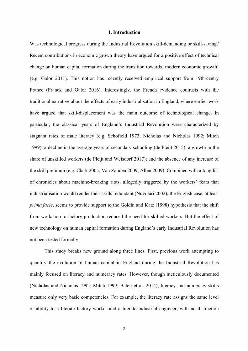
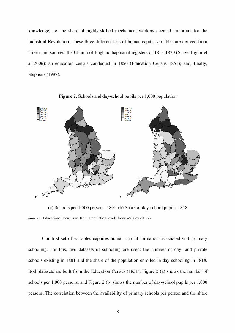
Figure 2. Schools and day-school pupils per 1,000 population

(a) Schools per 1,000 persons, 1801 (b) Share of day-school pupils, 1818

Sources: Educational Census of 1851. Population levels from Wrigley (2007).

Our first set of variables captures human capital formation associated with primary

schooling. For this, two datasets of schooling are used: the number of day- and private

schools existing in 1801 and the share of the population enrolled in day schooling in 1818.

Both datasets are built from the Education Census (1851). Figure 2 (a) shows the number of

schools per 1,000 persons, and Figure 2 (b) shows the number of day-school pupils per 1,000

persons. The correlation between the availability of primary schools per person and the share

9

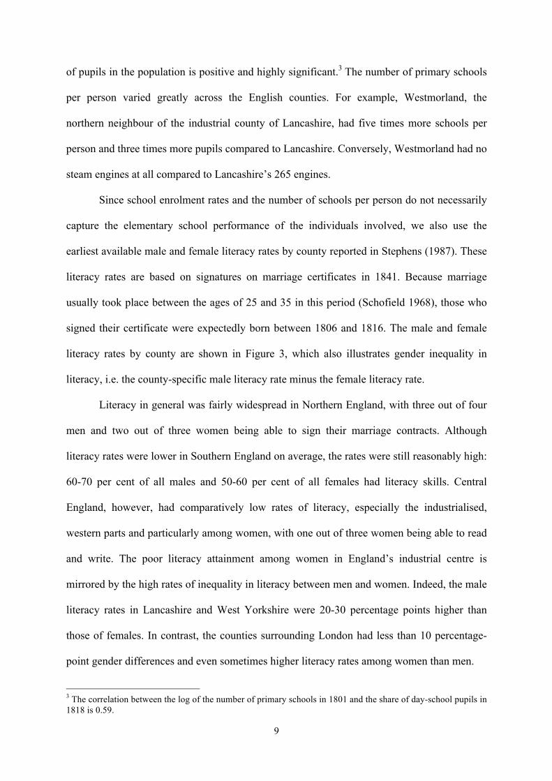
of pupils in the population is positive and highly significant.3 The number of primary schools

per person varied greatly across the English counties. For example, Westmorland, the

northern neighbour of the industrial county of Lancashire, had five times more schools per

person and three times more pupils compared to Lancashire. Conversely, Westmorland had no

steam engines at all compared to Lancashire’s 265 engines.

Since school enrolment rates and the number of schools per person do not necessarily

capture the elementary school performance of the individuals involved, we also use the

earliest available male and female literacy rates by county reported in Stephens (1987). These

literacy rates are based on signatures on marriage certificates in 1841. Because marriage

usually took place between the ages of 25 and 35 in this period (Schofield 1968), those who

signed their certificate were expectedly born between 1806 and 1816. The male and female

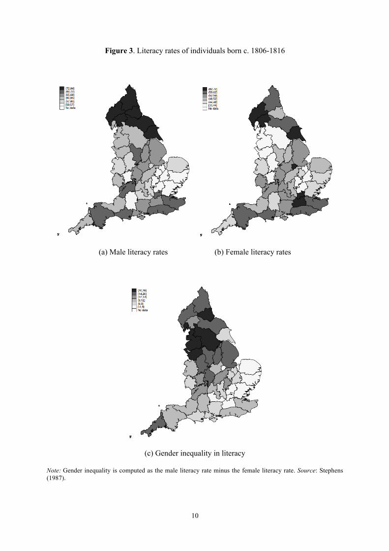
literacy rates by county are shown in Figure 3, which also illustrates gender inequality in

literacy, i.e. the county-specific male literacy rate minus the female literacy rate.

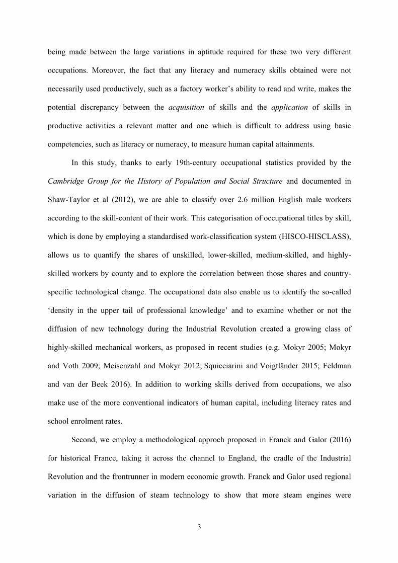
Literacy in general was fairly widespread in Northern England, with three out of four

men and two out of three women being able to sign their marriage contracts. Although

literacy rates were lower in Southern England on average, the rates were still reasonably high:

60-70 per cent of all males and 50-60 per cent of all females had literacy skills. Central

England, however, had comparatively low rates of literacy, especially the industrialised,

western parts and particularly among women, with one out of three women being able to read

and write. The poor literacy attainment among women in England’s industrial centre is

mirrored by the high rates of inequality in literacy between men and women. Indeed, the male

literacy rates in Lancashire and West Yorkshire were 20-30 percentage points higher than

those of females. In contrast, the counties surrounding London had less than 10 percentage-

point gender differences and even sometimes higher literacy rates among women than men.

3 The correlation between the log of the number of primary schools in 1801 and the share of day-school pupils in 1818 is 0.59.

10

Figure 3. Literacy rates of individuals born c. 1806-1816

(a) Male literacy rates (b) Female literacy rates

(c) Gender inequality in literacy

Note: Gender inequality is computed as the male literacy rate minus the female literacy rate. Source: Stephens (1987).

11

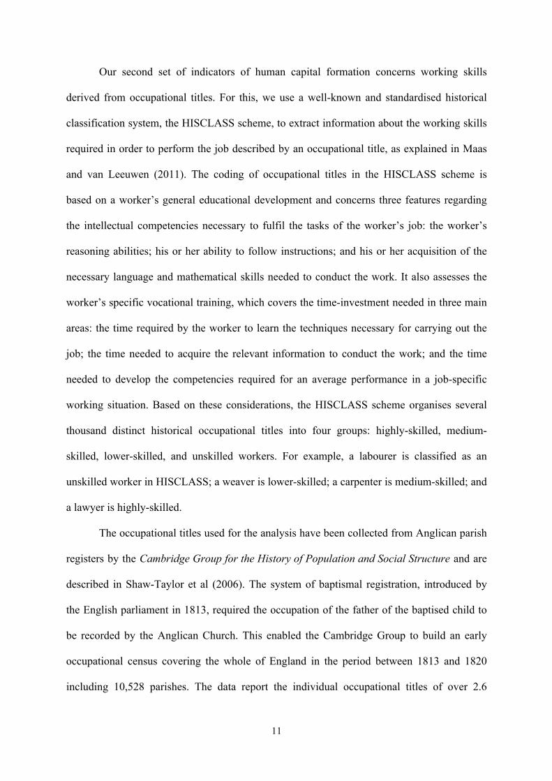
Our second set of indicators of human capital formation concerns working skills

derived from occupational titles. For this, we use a well-known and standardised historical

classification system, the HISCLASS scheme, to extract information about the working skills

required in order to perform the job described by an occupational title, as explained in Maas

and van Leeuwen (2011). The coding of occupational titles in the HISCLASS scheme is

based on a worker’s general educational development and concerns three features regarding

the intellectual competencies necessary to fulfil the tasks of the worker’s job: the worker’s

reasoning abilities; his or her ability to follow instructions; and his or her acquisition of the

necessary language and mathematical skills needed to conduct the work. It also assesses the

worker’s specific vocational training, which covers the time-investment needed in three main

areas: the time required by the worker to learn the techniques necessary for carrying out the

job; the time needed to acquire the relevant information to conduct the work; and the time

needed to develop the competencies required for an average performance in a job-specific

working situation. Based on these considerations, the HISCLASS scheme organises several

thousand distinct historical occupational titles into four groups: highly-skilled, medium-

skilled, lower-skilled, and unskilled workers. For example, a labourer is classified as an

unskilled worker in HISCLASS; a weaver is lower-skilled; a carpenter is medium-skilled; and

a lawyer is highly-skilled.

The occupational titles used for the analysis have been collected from Anglican parish

registers by the Cambridge Group for the History of Population and Social Structure and are

described in Shaw-Taylor et al (2006). The system of baptismal registration, introduced by

the English parliament in 1813, required the occupation of the father of the baptised child to

be recorded by the Anglican Church. This enabled the Cambridge Group to build an early

occupational census covering the whole of England in the period between 1813 and 1820

including 10,528 parishes. The data report the individual occupational titles of over 2.6

12

million adult males. Out of these we were able to classify some 1,700 distinct titles into one

of the four skill-categories described above, covering 99 per cent of the sampled adult males.4

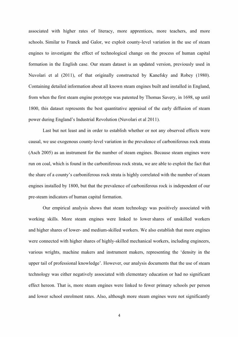
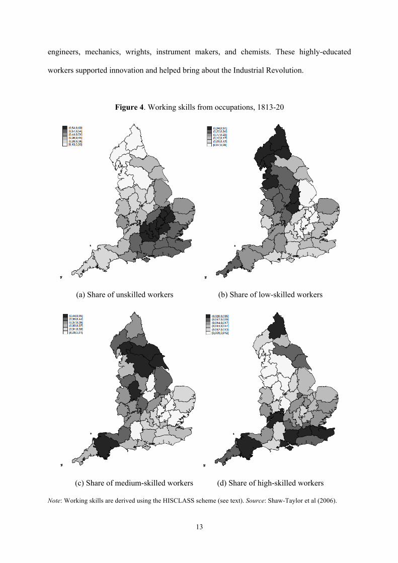
Figure 4 (a)-(d) shows the distribution of the working skill, by county, for each of the

four skill-categories. The overall patterns of the geographical distribution of working skills

were rather clear. Unskilled work (panel a) was more prevalent in South-East England and

was also concentrated to the north-west of London. For example, the agricultural county of

Hertfordshire, situated north of London, had 60 per cent of its workforce coded as unskilled.

By contrast, the industrial county of Cheshire had half as many coded as such, i.e. some 30

per cent. Lower- and medium-skilled work displayed a geographical pattern rather opposite to

that concerning unskilled work. Lower-skilled work (panel b) was mostly concentrated in the

west of England, particularly in the industrial centres and to the far north. The same is true of

medium-skilled work (panel c), which is also found in the industrial counties, with a very

high prevalence in Yorkshire West Riding. Unlike lower- and medium-skilled work, however,

highly-skilled work (panel d) was rather uncommon in England’s industrial centre and was

mostly a Southern England phenomenon, concentrated in Devon and south of London.

Two more indicators of human capital formation are introduced in order to try to

measure the industry-specific training of workers. The first measure concerns the share of

highly-skilled mechanical workmen. This is based on work by Mokyr and collaborators, who

have emphasised the importance of ‘the density in the upper tail of professional knowledge’

vis-à-vis the average level of human capital present in the workforce (Mokyr 2005; Mokyr

and Voth 2009; Feldman and Van Der Beek 2016). To follow Meisenzahl and Mokyr (2012),

it was not the average level of human capital that was important in the process of

industrialisation, but rather the upper tail of the human capital distribution, i.e. technological

change and the adoption of machinery affected the demand for high-quality workmen such as 4 ‘Gentleman’, ‘Esquire’, ‘Pauper’, ‘Widower’ and ‘Slave’ were excluded from the original data set. These titles, which make up some one per cent of the sampled population, do not refer to an actual profession and hence cannot be coded using the HISCLASS scheme.

13

engineers, mechanics, wrights, instrument makers, and chemists. These highly-educated

workers supported innovation and helped bring about the Industrial Revolution.

Figure 4. Working skills from occupations, 1813-20

(a) Share of unskilled workers (b) Share of low-skilled workers

(c) Share of medium-skilled workers (d) Share of high-skilled workers

Note: Working skills are derived using the HISCLASS scheme (see text). Source: Shaw-Taylor et al (2006).

14

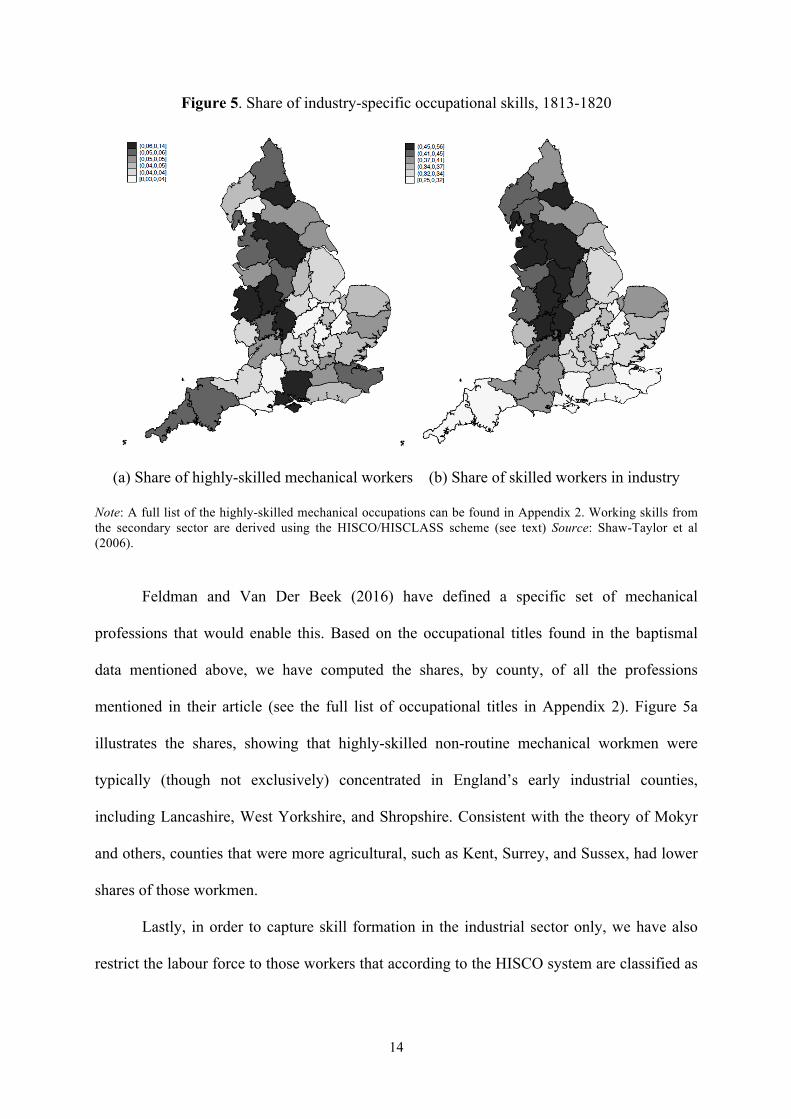
Figure 5. Share of industry-specific occupational skills, 1813-1820

(a) Share of highly-skilled mechanical workers (b) Share of skilled workers in industry

Note: A full list of the highly-skilled mechanical occupations can be found in Appendix 2. Working skills from the secondary sector are derived using the HISCO/HISCLASS scheme (see text) Source: Shaw-Taylor et al (2006).

Feldman and Van Der Beek (2016) have defined a specific set of mechanical

professions that would enable this. Based on the occupational titles found in the baptismal

data mentioned above, we have computed the shares, by county, of all the professions

mentioned in their article (see the full list of occupational titles in Appendix 2). Figure 5a

illustrates the shares, showing that highly-skilled non-routine mechanical workmen were

typically (though not exclusively) concentrated in England’s early industrial counties,

including Lancashire, West Yorkshire, and Shropshire. Consistent with the theory of Mokyr

and others, counties that were more agricultural, such as Kent, Surrey, and Sussex, had lower

shares of those workmen.

Lastly, in order to capture skill formation in the industrial sector only, we have also

restrict the labour force to those workers that according to the HISCO system are classified as

15

belonging to the secondary (i.e. industrial) sector. Their shares, by county, are illustrated in

Figure 5b and appear to concentrate in England’s industrial centres.

Our regression analysis below accounts for the confounding geographic and

institutional characteristics of each county, as well as their pre-industrial developments. All of

these characteristics may have contributed to industrialisation, as well as to the formation of

human capital. In particular, pre-industrial developments, such as the early growth of cities or

the prevalence of pre-industrial schools, may have helped encourage industrialisation and

education independently. Our first set of control variables capture the geographical

characteristics of the English counties. Specifically, regional differences in geography linked

to land quality and agricultural output may have affected the process of industrialisation

helping the adoption of steam engines. Land quality and output may also have affected

landownership and landowners’ attitudes regarding educational institutions and hence the

human capital formation of workers (Galor and Vollrath 2009). Our analysis accounts for this

by controlling for land quality, measured by land rents (Clark 2002), as well as climatic

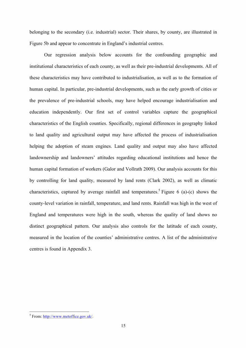
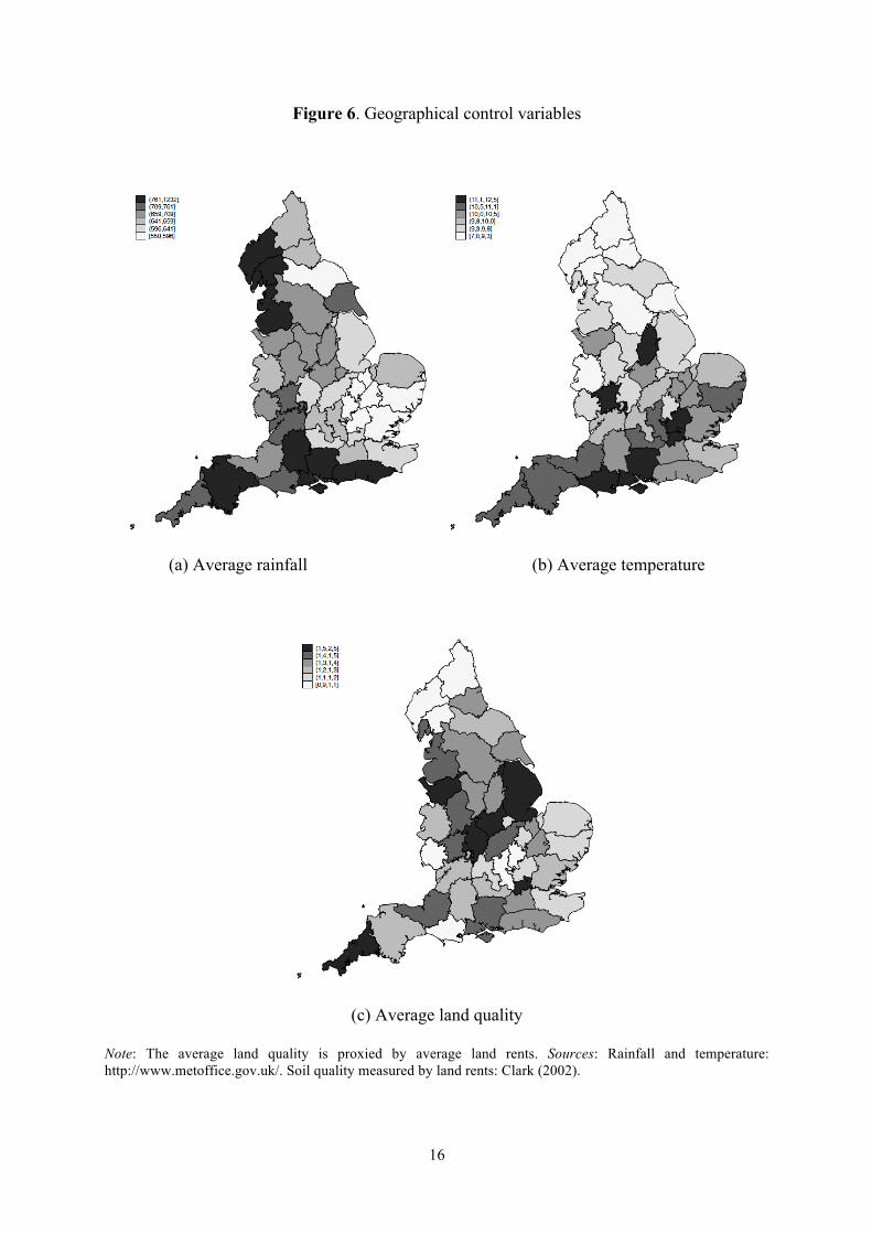
characteristics, captured by average rainfall and temperatures.5 Figure 6 (a)-(c) shows the

county-level variation in rainfall, temperature, and land rents. Rainfall was high in the west of

England and temperatures were high in the south, whereas the quality of land shows no

distinct geographical pattern. Our analysis also controls for the latitude of each county,

measured in the location of the counties’ administrative centres. A list of the administrative

centres is found in Appendix 3.

5 From: http://www.metoffice.gov.uk/.

16

Figure 6. Geographical control variables

(a) Average rainfall (b) Average temperature

(c) Average land quality

Note: The average land quality is proxied by average land rents. Sources: Rainfall and temperature: http://www.metoffice.gov.uk/. Soil quality measured by land rents: Clark (2002).

17

We also control for effects that might emerge as a result of the geographical location

of a county vis-à-vis the possibilities for foreign influences. Trade or various forms of cultural

impacts, stemming from contacts with non-nationals, may have stimulated the development of

industry or the formation of human capital. Our analysis controls for this by using dummy

variables accounting for counties that were bordering other countries (i.e. Wales or Scotland)

or had access to the sea (Maritime). Our study also controls for political institutions and their

influences on industry and human capital formation. For example, the English Parliament,

located in London, may have exercised a stronger influence on nearby counties than on

countries situated further away. The analysis accounts for such effects using dummy variables

for the counties surrounding London (i.e. Essex, Hertfordshire, Kent, Middlesex, and Surrey)

and for the aerial distance (in km) from London to the administrative centre of each county.

Finally, our study controls for the potential confounding effects stemming from

regional variation in developments achieved during the pre-industrial period. Counties that

had many primary and secondary schools (see Figures 7a and 7b) may have had higher levels

of pre-industrial human capital than others. Similarly, counties that were more urbanised

before the Industrial Revolution (see Figure 7c) may have been more likely to industrialise or

to successfully attract human capital. We therefore control for these pre-industrial

developments by accounting for the county-specific numbers of primary schools, taken from

the Schools Inquiry Commission (1868a), and secondary schools, taken from Schools Inquiry

Commission (1868b). We also control for the urbanisation ratio in 1700, which is defined as

the population in cities with more than 5,000 inhabitants divided by the total population.

These numbers were provided in Bosker et al (2012).

18

Figure 7. Pre-industrial developments

(a) Primary schools per 1,000 person, 1700 (b) Secondary schools per 1,000 person, 1700

(c) Urbanisation ratio, 1700

Note: The urbanisation ratio is the population in cities with more than 5,000 inhabitants divided by the total population. Sources: Primary schools from Schools Inquiry Commission (1868a) and secondary schools from Schools Inquiry Commission (1868b). Urbanisation rates from Bosker et al (2012).

19

3. Empirical analysis

What was the effect of early industrialisation on human capital formation in England? To find

out, we explore the empirical relationship between the county-level distribution of steam

engines and the indicators of human capital described above, while controlling for

confounding factors. Of course, an observed relationship between industrialisation and human

capital formation is not necessarily causal. The process of industrialisation and that of human

capital formation may have taken place independently, governed by common forces of

economic development. In order to deal with this potential issue of endogeneity, we use

exogenous variation in the distribution of carboniferous rock strata as an instrument for the

number of steam engines installed by 1800. Coal is often found in rock strata from the

Carboniferous age (360 to 300 million years ago). During this era, large forests covered the

areas that later on formed the earth’s coal layers. Coalfields therefore habitually emerged near

to rock strata from the Carboniferous epoch. Crafts and Malutu (2006) have shown that coal

abundance mattered for the location of steam-intensive industries, and Fernihough and

O’Rourke (2014) that it linked to industry. For instance, due to its absence of coal, the county

of Dorset was unable to compete with counties such as Lancashire and as a result remained

largely rural up until the present (Cullingford 1980). Below we will use the fact that the share

of a county’s carboniferous rock strata is highly correlated with the number of steam engines

built and installed by 1800, but that the concentration of rock is independent of the indicators

of pre-industrial development.

20

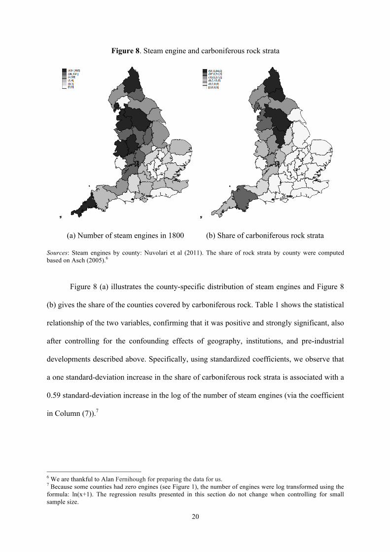
Figure 8. Steam engine and carboniferous rock strata

(a) Number of steam engines in 1800 (b) Share of carboniferous rock strata

Sources: Steam engines by county: Nuvolari et al (2011). The share of rock strata by county were computed based on Asch (2005).6

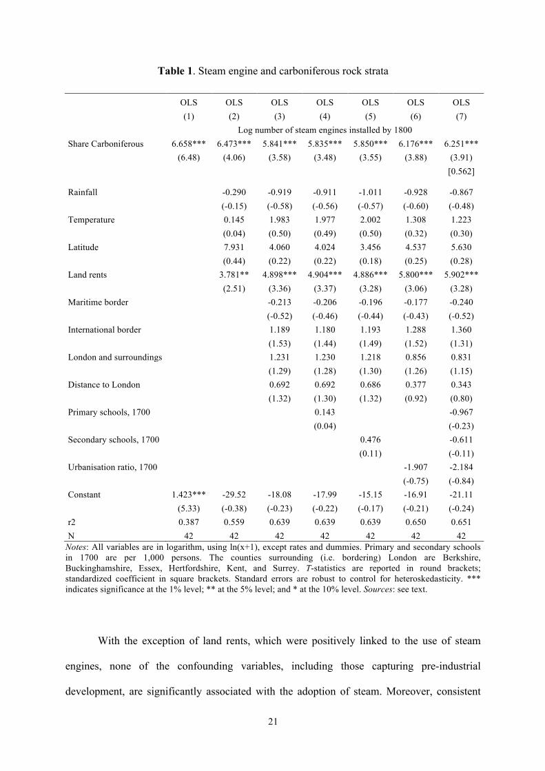
Figure 8 (a) illustrates the county-specific distribution of steam engines and Figure 8

(b) gives the share of the counties covered by carboniferous rock. Table 1 shows the statistical

relationship of the two variables, confirming that it was positive and strongly significant, also

after controlling for the confounding effects of geography, institutions, and pre-industrial

developments described above. Specifically, using standardized coefficients, we observe that

a one standard-deviation increase in the share of carboniferous rock strata is associated with a

0.59 standard-deviation increase in the log of the number of steam engines (via the coefficient

in Column (7)).7

6 We are thankful to Alan Fernihough for preparing the data for us. 7 Because some counties had zero engines (see Figure 1), the number of engines were log transformed using the formula: ln(x+1). The regression results presented in this section do not change when controlling for small sample size.

21

Table 1. Steam engine and carboniferous rock strata

OLS OLS OLS OLS OLS OLS OLS

(1) (2) (3) (4) (5) (6) (7)

Log number of steam engines installed by 1800

Share Carboniferous 6.658*** 6.473*** 5.841*** 5.835*** 5.850*** 6.176*** 6.251***

(6.48) (4.06) (3.58) (3.48) (3.55) (3.88) (3.91)

[0.562] Rainfall

-0.290 -0.919 -0.911 -1.011 -0.928 -0.867

(-0.15) (-0.58) (-0.56) (-0.57) (-0.60) (-0.48)

Temperature

0.145 1.983 1.977 2.002 1.308 1.223

(0.04) (0.50) (0.49) (0.50) (0.32) (0.30)

Latitude

7.931 4.060 4.024 3.456 4.537 5.630

(0.44) (0.22) (0.22) (0.18) (0.25) (0.28)

Land rents

3.781** 4.898*** 4.904*** 4.886*** 5.800*** 5.902***

(2.51) (3.36) (3.37) (3.28) (3.06) (3.28)

Maritime border

-0.213 -0.206 -0.196 -0.177 -0.240

(-0.52) (-0.46) (-0.44) (-0.43) (-0.52)

International border

1.189 1.180 1.193 1.288 1.360

(1.53) (1.44) (1.49) (1.52) (1.31)

London and surroundings

1.231 1.230 1.218 0.856 0.831

(1.29) (1.28) (1.30) (1.26) (1.15)

Distance to London

0.692 0.692 0.686 0.377 0.343

(1.32) (1.30) (1.32) (0.92) (0.80)

Primary schools, 1700

0.143

-0.967

(0.04)

(-0.23)

Secondary schools, 1700

0.476

-0.611

(0.11)

(-0.11)

Urbanisation ratio, 1700

-1.907 -2.184

(-0.75) (-0.84)

Constant 1.423*** -29.52 -18.08 -17.99 -15.15 -16.91 -21.11

(5.33) (-0.38) (-0.23) (-0.22) (-0.17) (-0.21) (-0.24)

r2 0.387 0.559 0.639 0.639 0.639 0.650 0.651 N 42 42 42 42 42 42 42

Notes: All variables are in logarithm, using ln(x+1), except rates and dummies. Primary and secondary schools in 1700 are per 1,000 persons. The counties surrounding (i.e. bordering) London are Berkshire, Buckinghamshire, Essex, Hertfordshire, Kent, and Surrey. T-statistics are reported in round brackets; standardized coefficient in square brackets. Standard errors are robust to control for heteroskedasticity. *** indicates significance at the 1% level; ** at the 5% level; and * at the 10% level. Sources: see text.

With the exception of land rents, which were positively linked to the use of steam

engines, none of the confounding variables, including those capturing pre-industrial

development, are significantly associated with the adoption of steam. Moreover, consistent

22

with this relationship, the three counties with the most steam engines, i.e. West Yorkshire,

Lancashire, and Northumberland, had some of the highest share of carboniferous rock,

ranging between 50 and 80 per cent of the county’s surface area. There were 15 counties that

had more than 20 steam engines, and only one of these had no carboniferous rock. For each of

the remaining 14 counties, at least one third of the area had carboniferous rock strata. By

contrast, 10 out of those 11 counties that had no steam engines also had no carboniferous rock

at all (see also Figure 1).

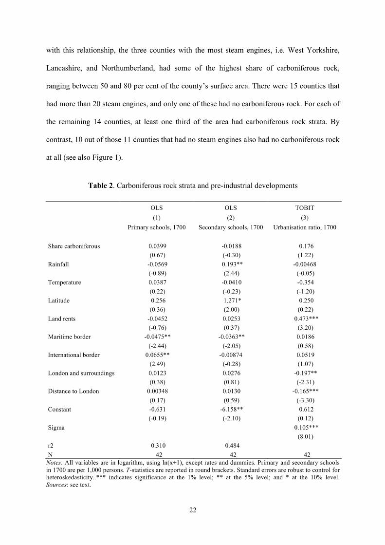
Table 2. Carboniferous rock strata and pre-industrial developments

OLS OLS TOBIT

(1) (2) (3)

Primary schools, 1700 Secondary schools, 1700 Urbanisation ratio, 1700

Share carboniferous 0.0399 -0.0188 0.176

(0.67) (-0.30) (1.22)

Rainfall -0.0569 0.193** -0.00468

(-0.89) (2.44) (-0.05)

Temperature 0.0387 -0.0410 -0.354

(0.22) (-0.23) (-1.20)

Latitude 0.256 1.271* 0.250

(0.36) (2.00) (0.22)

Land rents -0.0452 0.0253 0.473***

(-0.76) (0.37) (3.20)

Maritime border -0.0475** -0.0363** 0.0186

(-2.44) (-2.05) (0.58)

International border 0.0655** -0.00874 0.0519

(2.49) (-0.28) (1.07)

London and surroundings 0.0123 0.0276 -0.197**

(0.38) (0.81) (-2.31)

Distance to London 0.00348 0.0130 -0.165***

(0.17) (0.59) (-3.30)

Constant -0.631 -6.158** 0.612

(-0.19) (-2.10) (0.12)

Sigma 0.105***

(8.01)

r2 0.310 0.484 N 42 42 42

Notes: All variables are in logarithm, using ln(x+1), except rates and dummies. Primary and secondary schools in 1700 are per 1,000 persons. T-statistics are reported in round brackets. Standard errors are robust to control for heteroskedasticity..*** indicates significance at the 1% level; ** at the 5% level; and * at the 10% level. Sources: see text.

23

The validity of using the distribution of carboniferous rock as an instrument for the

distribution of steam engines is increased by the fact that rock strata is not significantly

correlated with pre-industrial developments. Table 2 shows that there is no statistically

significant association between the share of carboniferous rock and the number of primary

schools per 1,000 person in 1700 (Column 1); the number of secondary schools per 1,000

person in 1700 (Column 2); or the urbanisation ratio in 1700 (Column 3). Table 2 also shows

why it is vital to control for geography and institutions, which in many cases link to pre-

industrial development.

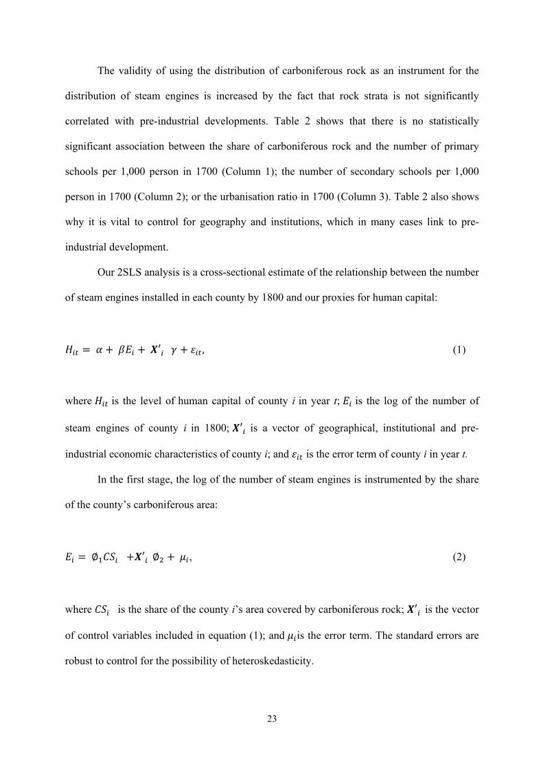
Our 2SLS analysis is a cross-sectional estimate of the relationship between the number

of steam engines installed in each county by 1800 and our proxies for human capital:

𝐻!" = 𝛼 + 𝛽𝐸! + 𝑿′! 𝛾 + 𝜀!" , (1)

where 𝐻!" is the level of human capital of county i in year t; 𝐸! is the log of the number of

steam engines of county i in 1800; 𝑿′! is a vector of geographical, institutional and pre-

industrial economic characteristics of county i; and 𝜀!" is the error term of county i in year t.

In the first stage, the log of the number of steam engines is instrumented by the share

of the county’s carboniferous area:

𝐸! = ∅!𝐶𝑆! +𝑿′! ∅! + 𝜇!, (2)

where 𝐶𝑆! is the share of the county i’s area covered by carboniferous rock; 𝑿′! is the vector

of control variables included in equation (1); and 𝜇!is the error term. The standard errors are

robust to control for the possibility of heteroskedasticity.

24

3.1 Working skills

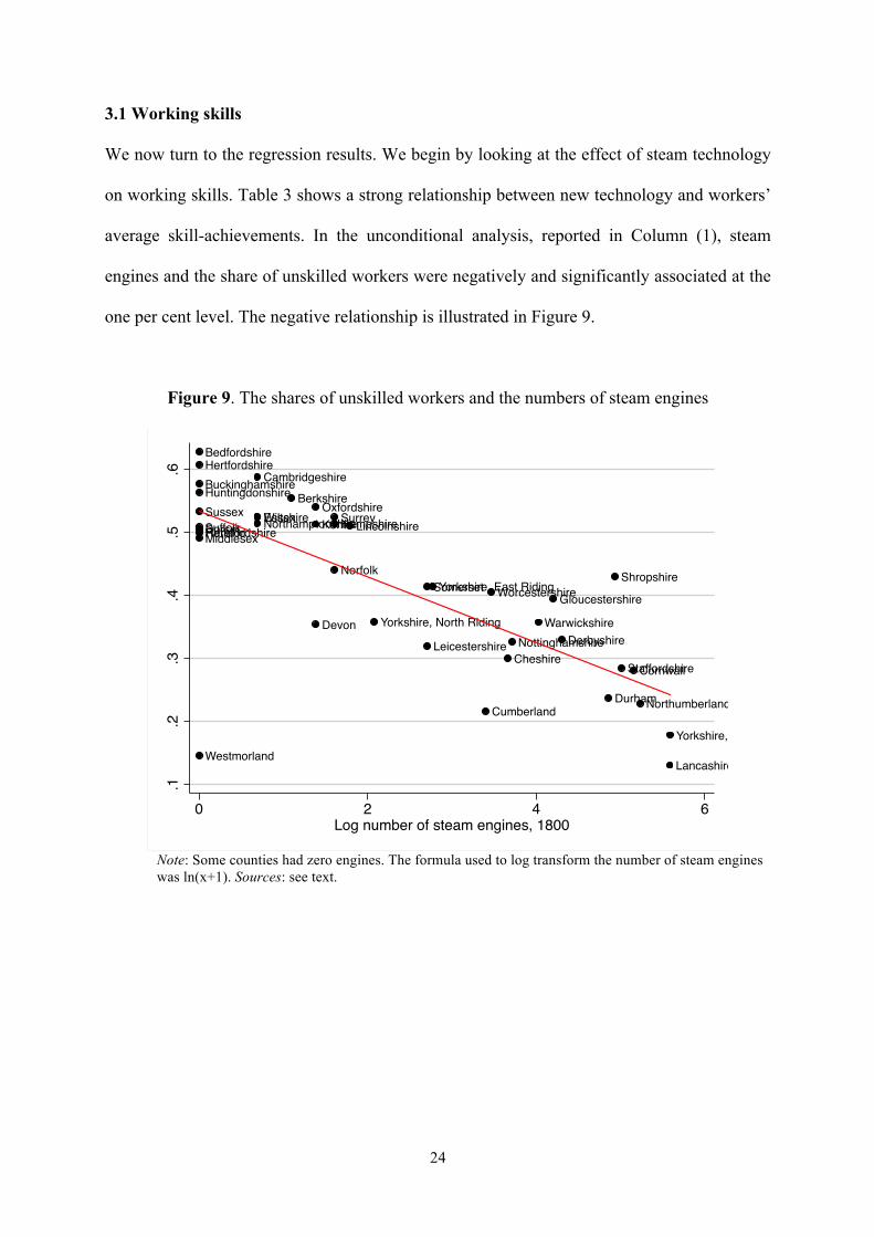
We now turn to the regression results. We begin by looking at the effect of steam technology

on working skills. Table 3 shows a strong relationship between new technology and workers’

average skill-achievements. In the unconditional analysis, reported in Column (1), steam

engines and the share of unskilled workers were negatively and significantly associated at the

one per cent level. The negative relationship is illustrated in Figure 9.

Figure 9. The shares of unskilled workers and the numbers of steam engines

Note: Some counties had zero engines. The formula used to log transform the number of steam engines was ln(x+1). Sources: see text.

Bedfordshire

BerkshireBuckinghamshireCambridgeshire

CheshireCornwall

Cumberland

DerbyshireDevon

Dorset

Durham

Essex

Gloucestershire

HampshireHerefordshire

Hertfordshire

Huntingdonshire

Kent

Lancashire

Leicestershire

LincolnshireMiddlesex

Norfolk

Northamptonshire

Northumberland

Nottinghamshire

Oxfordshire

Rutland

ShropshireSomerset

Staffordshire

SuffolkSurreySussex

Warwickshire

Westmorland

Wiltshire

WorcestershireYorkshire, East Riding

Yorkshire, North Riding

Yorkshire, West Riding

.1.2

.3.4

.5.6

0 2 4 6Log number of steam engines, 1800

25

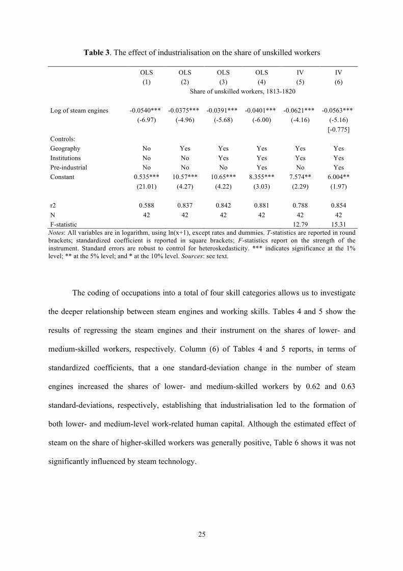
Table 3. The effect of industrialisation on the share of unskilled workers

OLS OLS OLS OLS IV IV

(1) (2) (3) (4) (5) (6)

Share of unskilled workers, 1813-1820

Log of steam engines -0.0540*** -0.0375*** -0.0391*** -0.0401*** -0.0621*** -0.0563***

(-6.97) (-4.96) (-5.68) (-6.00) (-4.16) (-5.16)

[-0.775] Controls:

Geography No Yes Yes Yes Yes Yes Institutions No No Yes Yes Yes Yes Pre-industrial No No No Yes No Yes Constant 0.535*** 10.57*** 10.65*** 8.355*** 7.574** 6.004**

(21.01) (4.27) (4.22) (3.03) (2.29) (1.97)

r2 0.588 0.837 0.842 0.881 0.788 0.854 N 42 42 42 42 42 42 F-statistic 12.79 15.31

Notes: All variables are in logarithm, using ln(x+1), except rates and dummies. T-statistics are reported in round brackets; standardized coefficient is reported in square brackets; F-statistics report on the strength of the instrument. Standard errors are robust to control for heteroskedasticity. *** indicates significance at the 1% level; ** at the 5% level; and * at the 10% level. Sources: see text.

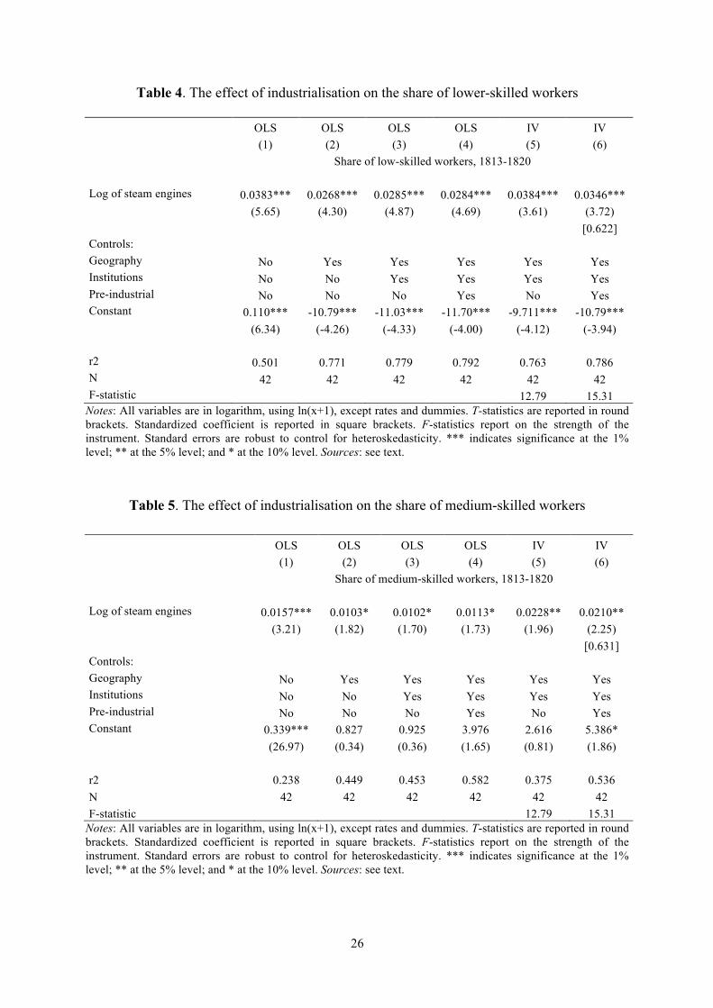
The coding of occupations into a total of four skill categories allows us to investigate

the deeper relationship between steam engines and working skills. Tables 4 and 5 show the

results of regressing the steam engines and their instrument on the shares of lower- and

medium-skilled workers, respectively. Column (6) of Tables 4 and 5 reports, in terms of

standardized coefficients, that a one standard-deviation change in the number of steam

engines increased the shares of lower- and medium-skilled workers by 0.62 and 0.63

standard-deviations, respectively, establishing that industrialisation led to the formation of

both lower- and medium-level work-related human capital. Although the estimated effect of

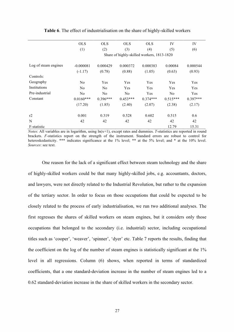
steam on the share of higher-skilled workers was generally positive, Table 6 shows it was not

significantly influenced by steam technology.

26

Table 4. The effect of industrialisation on the share of lower-skilled workers


(1) (2) (3) (4) (5) (6)

Share of low-skilled workers, 1813-1820

Log of steam engines 0.0383*** 0.0268*** 0.0285*** 0.0284*** 0.0384*** 0.0346***

(5.65) (4.30) (4.87) (4.69) (3.61) (3.72)

[0.622] Controls:

Geography No Yes Yes Yes Yes Yes Institutions No No Yes Yes Yes Yes Pre-industrial No No No Yes No Yes Constant 0.110*** -10.79*** -11.03*** -11.70*** -9.711*** -10.79***

(6.34) (-4.26) (-4.33) (-4.00) (-4.12) (-3.94)

r2 0.501 0.771 0.779 0.792 0.763 0.786 N 42 42 42 42 42 42 F-statistic 12.79 15.31

Notes: All variables are in logarithm, using ln(x+1), except rates and dummies. T-statistics are reported in round brackets. Standardized coefficient is reported in square brackets. F-statistics report on the strength of the instrument. Standard errors are robust to control for heteroskedasticity. *** indicates significance at the 1% level; ** at the 5% level; and * at the 10% level. Sources: see text.

Table 5. The effect of industrialisation on the share of medium-skilled workers


(1) (2) (3) (4) (5) (6)

Share of medium-skilled workers, 1813-1820

Log of steam engines 0.0157*** 0.0103* 0.0102* 0.0113* 0.0228** 0.0210**

(3.21) (1.82) (1.70) (1.73) (1.96) (2.25)

[0.631] Controls:

Geography No Yes Yes Yes Yes Yes Institutions No No Yes Yes Yes Yes Pre-industrial No No No Yes No Yes Constant 0.339*** 0.827 0.925 3.976 2.616 5.386*

(26.97) (0.34) (0.36) (1.65) (0.81) (1.86)

r2 0.238 0.449 0.453 0.582 0.375 0.536 N 42 42 42 42 42 42 F-statistic 12.79 15.31


27

Table 6. The effect of industrialisation on the share of highly-skilled workers


(1) (2) (3) (4) (5) (6)

Share of highly-skilled workers, 1813-1820

Log of steam engines -0.000081 0.000429 0.000372 0.000383 0.00084 0.000544

(-1.17) (0.78) (0.88) (1.05) (0.63) (0.93)

Controls: Geography No Yes Yes Yes Yes Yes

Institutions No No Yes Yes Yes Yes Pre-industrial No No No Yes No Yes Constant 0.0160*** 0.396*** 0.453*** 0.374*** 0.515*** 0.397***

(17.20) (1.85) (2.40) (2.07) (2.38) (2.17)

r2 0.001 0.319 0.528 0.602 0.515 0.6 N 42 42 42 42 42 42 F-statistic

12.79 15.31

Notes: All variables are in logarithm, using ln(x+1), except rates and dummies. T-statistics are reported in round brackets. F-statistics report on the strength of the instrument. Standard errors are robust to control for heteroskedasticity. *** indicates significance at the 1% level; ** at the 5% level; and * at the 10% level. Sources: see text.

One reason for the lack of a significant effect between steam technology and the share

of highly-skilled workers could be that many highly-skilled jobs, e.g. accountants, doctors,

and lawyers, were not directly related to the Industrial Revolution, but rather to the expansion

of the tertiary sector. In order to focus on those occupations that could be expected to be

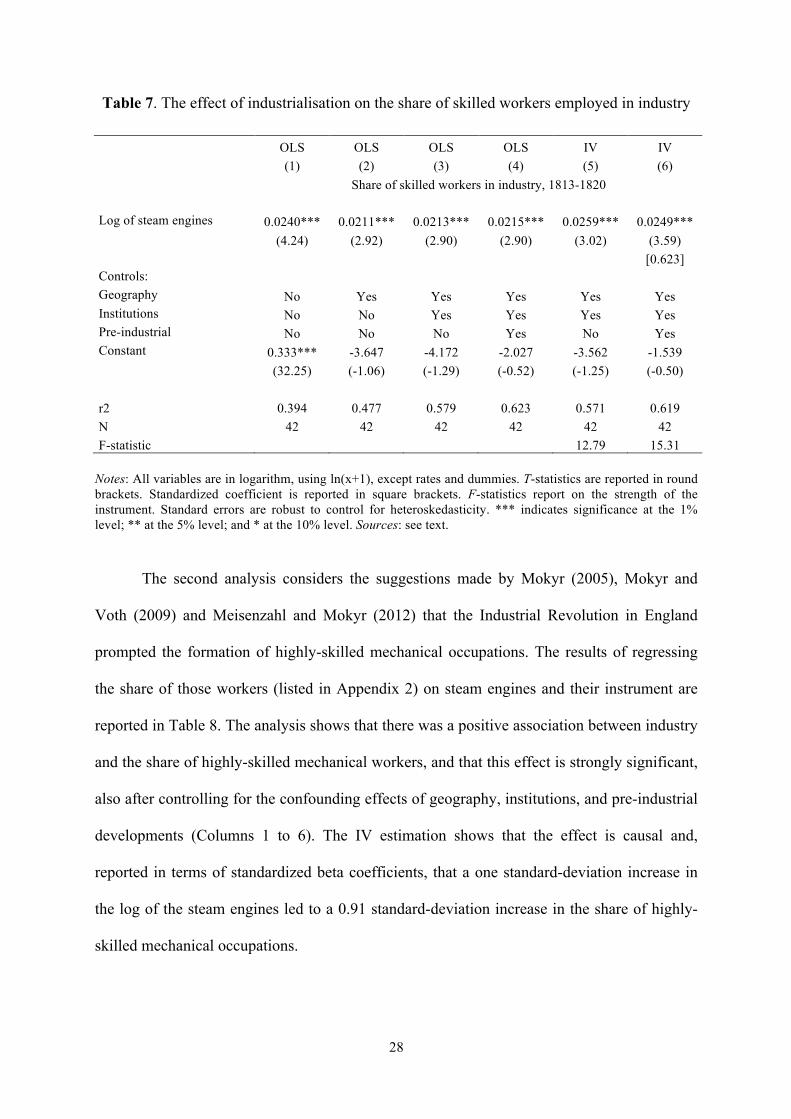
closely related to the process of early industrialisation, we run two additional analyses. The

first regresses the shares of skilled workers on steam engines, but it considers only those

occupations that belonged to the secondary (i.e. industrial) sector, including occupational

titles such as ‘cooper’, ‘weaver’, ‘spinner’, ‘dyer’ etc. Table 7 reports the results, finding that

the coefficient on the log of the number of steam engines is statistically significant at the 1%

level in all regressions. Column (6) shows, when reported in terms of standardized

coefficients, that a one standard-deviation increase in the number of steam engines led to a

0.62 standard-deviation increase in the share of skilled workers in the secondary sector.

28

Table 7. The effect of industrialisation on the share of skilled workers employed in industry


(1) (2) (3) (4) (5) (6)

Share of skilled workers in industry, 1813-1820


(4.24) (2.92) (2.90) (2.90) (3.02) (3.59)

[0.623] Controls:

Geography No Yes Yes Yes Yes Yes Institutions No No Yes Yes Yes Yes Pre-industrial No No No Yes No Yes Constant 0.333*** -3.647 -4.172 -2.027 -3.562 -1.539

(32.25) (-1.06) (-1.29) (-0.52) (-1.25) (-0.50)

r2 0.394 0.477 0.579 0.623 0.571 0.619 N 42 42 42 42 42 42 F-statistic 12.79 15.31


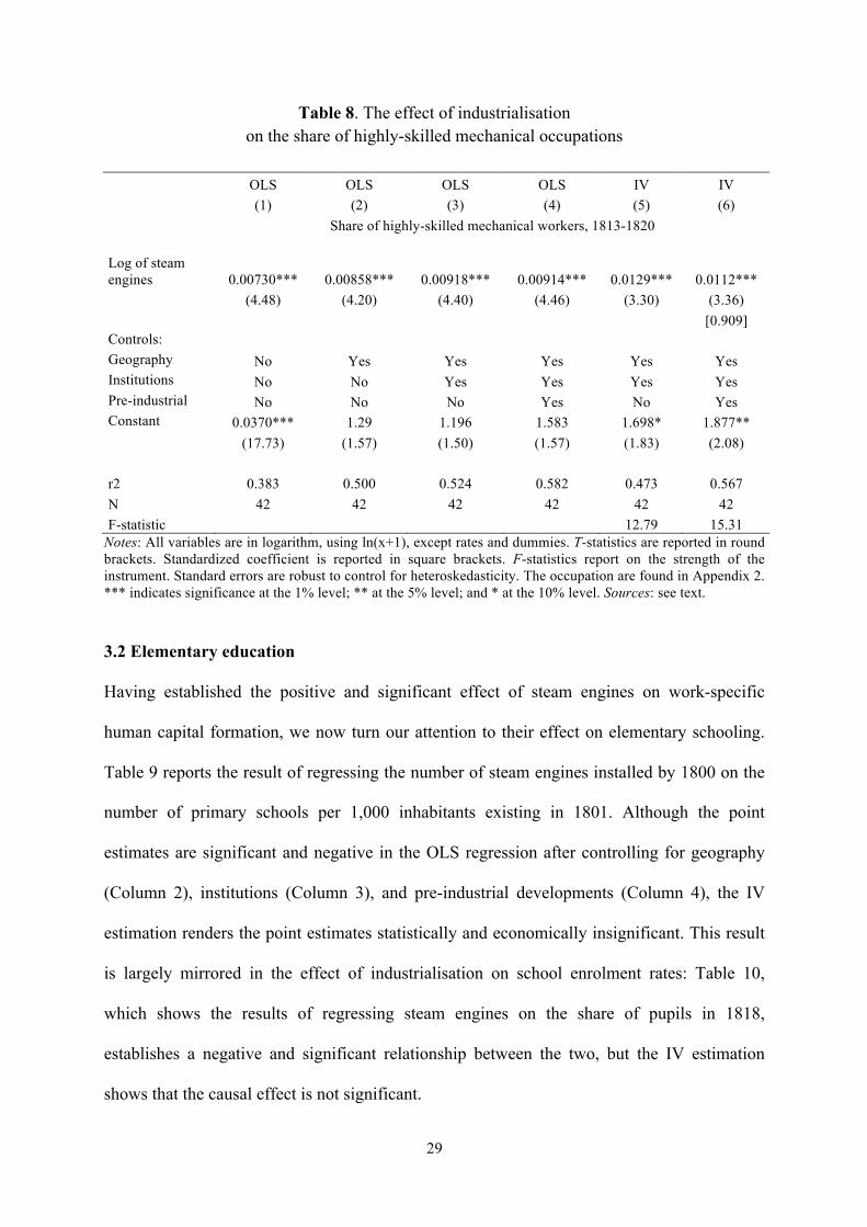
The second analysis considers the suggestions made by Mokyr (2005), Mokyr and

Voth (2009) and Meisenzahl and Mokyr (2012) that the Industrial Revolution in England

prompted the formation of highly-skilled mechanical occupations. The results of regressing

the share of those workers (listed in Appendix 2) on steam engines and their instrument are

reported in Table 8. The analysis shows that there was a positive association between industry

and the share of highly-skilled mechanical workers, and that this effect is strongly significant,

also after controlling for the confounding effects of geography, institutions, and pre-industrial

developments (Columns 1 to 6). The IV estimation shows that the effect is causal and,

reported in terms of standardized beta coefficients, that a one standard-deviation increase in

the log of the steam engines led to a 0.91 standard-deviation increase in the share of highly-

skilled mechanical occupations.

29

Table 8. The effect of industrialisation on the share of highly-skilled mechanical occupations


(1) (2) (3) (4) (5) (6)

Share of highly-skilled mechanical workers, 1813-1820


(4.48) (4.20) (4.40) (4.46) (3.30) (3.36)

[0.909] Controls:

Geography No Yes Yes Yes Yes Yes Institutions No No Yes Yes Yes Yes Pre-industrial No No No Yes No Yes Constant 0.0370*** 1.29 1.196 1.583 1.698* 1.877**

(17.73) (1.57) (1.50) (1.57) (1.83) (2.08)

r2 0.383 0.500 0.524 0.582 0.473 0.567 N 42 42 42 42 42 42 F-statistic 12.79 15.31

Notes: All variables are in logarithm, using ln(x+1), except rates and dummies. T-statistics are reported in round brackets. Standardized coefficient is reported in square brackets. F-statistics report on the strength of the instrument. Standard errors are robust to control for heteroskedasticity. The occupation are found in Appendix 2. *** indicates significance at the 1% level; ** at the 5% level; and * at the 10% level. Sources: see text.

3.2 Elementary education

Having established the positive and significant effect of steam engines on work-specific

human capital formation, we now turn our attention to their effect on elementary schooling.

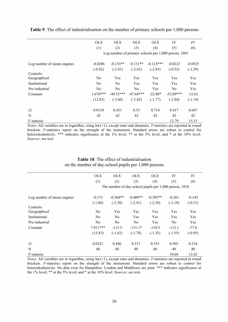
Table 9 reports the result of regressing the number of steam engines installed by 1800 on the

number of primary schools per 1,000 inhabitants existing in 1801. Although the point

estimates are significant and negative in the OLS regression after controlling for geography

(Column 2), institutions (Column 3), and pre-industrial developments (Column 4), the IV

estimation renders the point estimates statistically and economically insignificant. This result

is largely mirrored in the effect of industrialisation on school enrolment rates: Table 10,

which shows the results of regressing steam engines on the share of pupils in 1818,

establishes a negative and significant relationship between the two, but the IV estimation

shows that the causal effect is not significant.

30

Table 9. The effect of industrialisation on the number of primary schools per 1,000 persons


(1) (2) (3) (4) (5) (6)

Log number of primary schools per 1,000 person, 1801

Log number of steam engines -0.0286 -0.133** -0.131** -0.123*** -0.0223 -0.0525

(-0.82) (-2.41) (-2.43) (-2.85) (-0.52) (-1.29)

Controls: Geographical No Yes Yes Yes Yes Yes Institutional No No Yes Yes Yes Yes Pre-industrial No No No Yes No Yes Constant 1.676*** -49.53*** -47.64*** -22.88* -33.09*** -12.62

(12.83) (-3.46) (-3.42) (-1.77) (-2.84) (-1.14)

r2 0.0154 0.431 0.53 0.714 0.417 0.667 N 42 42 42 42 42 42 F-statistic 12.79 15.31

Notes: All variables are in logarithm, using ln(x+1), except rates and dummies. T-statistics are reported in round brackets. F-statistics report on the strength of the instrument. Standard errors are robust to control for heteroskedasticity. *** indicates significance at the 1% level; ** at the 5% level; and * at the 10% level. Sources: see text.

Table 10. The effect of industrialisation on the number of day-school pupils per 1,000 persons


(1) (2) (3) (4) (5) (6)

The number of day-school pupils per 1,000 person, 1818

Log number of steam engines -0.171 -0.360** -0.409** -0.395** -0.261 -0.145

(-1.06) (-2.30) (-2.41) (-2.30) (-1.18) (-0.53)

Controls: Geographical No Yes Yes Yes Yes Yes Institutional No No Yes Yes Yes Yes Pre-industrial No No No Yes No Yes Constant 7.911*** -113.5 -131.1* -110.5 -112.1 -77.6

(15.83) (-1.62) (-1.78) (-1.35) (-1.55) (-0.95)

r2 0.0321 0.446 0.517 0.555 0.505 0.524 N 40 40 40 40 40 40 F-statistic 10.68 12.62

Notes: All variables are in logarithm, using ln(x+1), except rates and dummies. T-statistics are reported in round brackets. F-statistics report on the strength of the instrument. Standard errors are robust to control for heteroskedasticity. No data exist for Hampshire. London and Middlesex are joint. *** indicates significance at the 1% level; ** at the 5% level; and * at the 10% level. Sources: see text.

31

Table 11. The effect of industrialisation on male literacy


(1) (2) (3) (4) (5) (6)

Male literacy rate of individuals born c. 1806-1816

Log number of steam engines 1.245* 0.0937 -0.0368 0.18 1.454 0.928

(1.77) (0.14) (-0.05) (0.25) (1.15) (0.88)

Controls: Geographical No Yes Yes Yes Yes Yes Institutional No No Yes Yes Yes Yes Pre-industrial No No No Yes No Yes Constant 62.28*** -337.0 -285.5 -322.0 -93.2 -223.6

(30.77) (-0.88) (-0.78) (-0.77) (-0.24) (-0.53)

r2 0.0781 0.352 0.469 0.516 0.417 0.503 N 41 41 41 41 41 41 F-statistic 10.49 12.83

Notes: All variables are in logarithm, using ln(x+1), except rates and dummies. T-statistics are reported in round brackets. F-statistics report on the strength of the instrument. Standard errors are robust to control for heteroskedasticity. London and Middelsex are joint. *** indicates significance at the 1% level; ** at the 5% level; and * at the 10% level. Sources: see text.

Table 12. The effect of industrialisation on female literacy


(1) (2) (3) (4) (5) (6)

Female literacy rate of individuals born c. 1806-1816

Log number of steam engines -1.360* -1.898** -1.679 -1.293 -1.54 -1.889

(-1.75) (-2.30) (-1.60) (-1.34) (-0.91) (-1.27)

Controls: Geographical No Yes Yes Yes Yes Yes Institutional No No Yes Yes Yes Yes Pre-industrial No No No Yes No Yes Constant 55.60*** 143.5 228.7 222.3 246.7 143.8

(26.51) (0.34) (0.52) (0.47) (0.55) (0.30)

r2 0.0813 0.19 0.299 0.372 0.299 0.365 N 41 41 41 41 41 41 F-statistic 10.49 12.83

Notes: All variables are in logarithm, using ln(x+1), except rates and dummies. T-statistics are reported in round brackets. F-statistics report on the strength of the instrument. Standard errors are robust to control for heteroskedasticity. London and Middelsex are joint. *** indicates significance at the 1% level; ** at the 5% level; and * at the 10% level. Sources: see text.

32

Table 13. The effect of industrialisation on gender inequality in literacy


(1) (2) (3) (4) (5) (6)

Gender inequality among individuals born c. 1806-1816

Log number of steam engines 2.606*** 1.562*** 1.643*** 1.473*** 2.994*** 2.817***

(6.61) (3.64) (3.64) (3.05) (3.51) (3.79)

[0.794] Controls: Geographical No Yes Yes Yes Yes Yes Institutional No No Yes Yes Yes Yes Pre-industrial No No No Yes No Yes Constant 6.672*** -504.8*** -514.1*** -544.3*** -339.9* -367.5**

(6.13) (-2.98) (-3.09) (-3.08) (-1.93) (-2.16)

r2 0.557 0.693 0.697 0.727 0.628 0.661 N 41 41 41 41 41 41 F-statistic 10.49 12.83

Note: Gender inequality is computed as the male literacy rate minus the female literacy rate. Notes: All variables are in logarithm, using ln(x+1), except rates and dummies. T-statistics are reported in round brackets. Standardized coefficient is reported in square brackets. F-statistics report on the strength of the instrument. Standard errors are robust to control for heteroskedasticity. London and Middelsex are joint. *** indicates significance at the 1% level; ** at the 5% level; and * at the 10% level. Sources: see text.

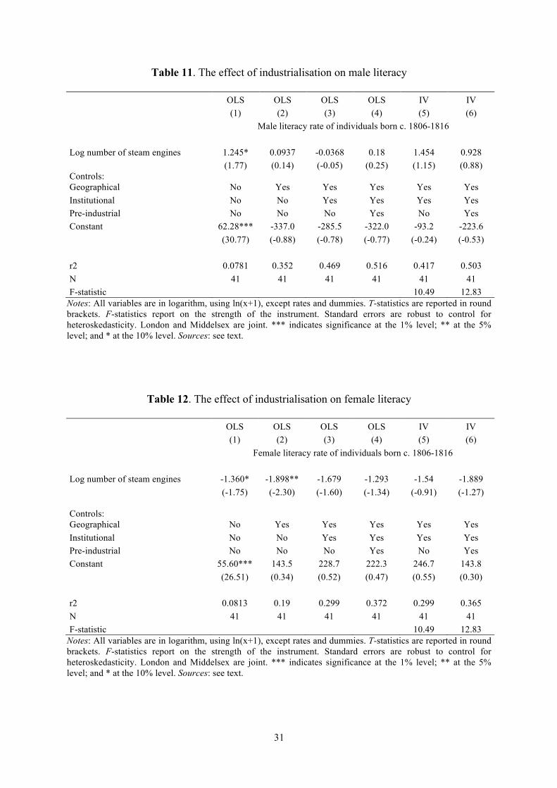
The relationships between industrialisation and male and female literacy attainment

are reported in Tables 11 and 12, respectively. Consistent with the IV analysis above

regarding school enrolment rates and the number of schools per person, the IV regression

results in Tables 11 and 12 show that more steam engines are not significantly associated with

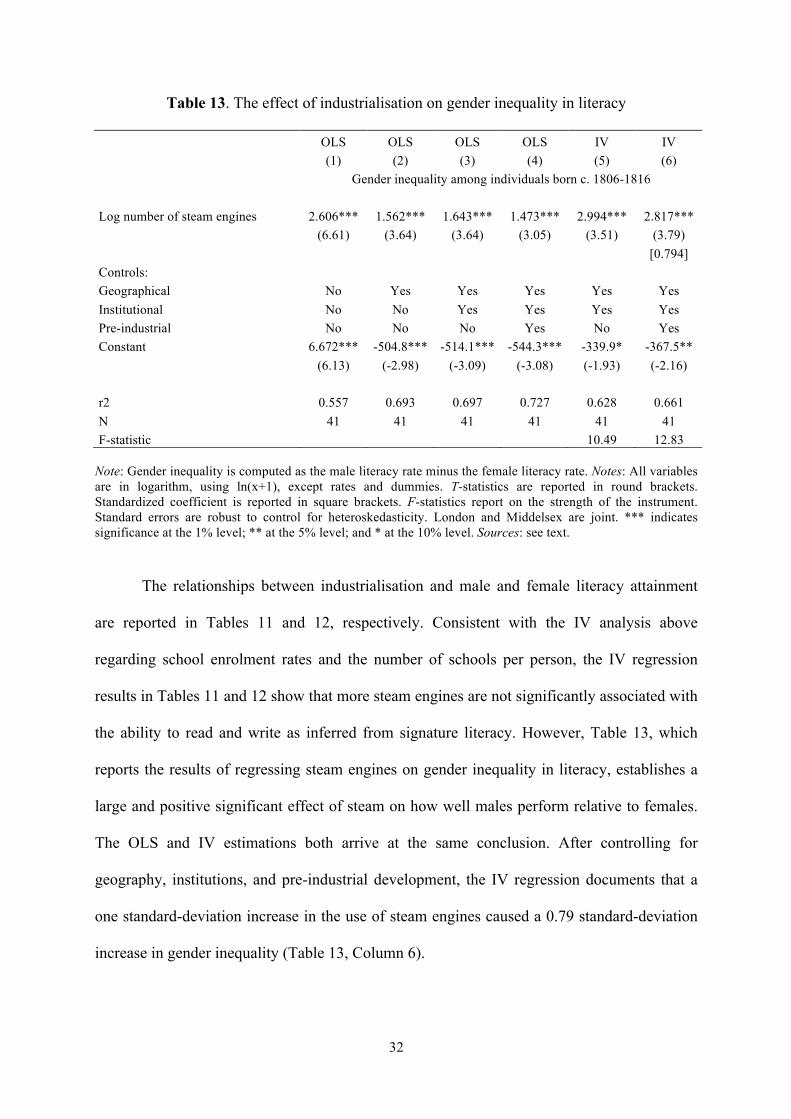
the ability to read and write as inferred from signature literacy. However, Table 13, which

reports the results of regressing steam engines on gender inequality in literacy, establishes a

large and positive significant effect of steam on how well males perform relative to females.

The OLS and IV estimations both arrive at the same conclusion. After controlling for

geography, institutions, and pre-industrial development, the IV regression documents that a

one standard-deviation increase in the use of steam engines caused a 0.79 standard-deviation

increase in gender inequality (Table 13, Column 6).

33

Overall the analyses of the effect of new industrial technology on literacy, as well as

schools and school enrolment rates, leave the impression that England’s Industrial Revolution

had no influence on the formation of elementary education. These findings chime well with

the earlier analysis of Humphries (2010) showing that industrialisation led to a decrease in

average years of schooling. They also correspond with previous work that has documented a

stagnant literacy rate of men during the classic period of the Industrial Revolution (e.g.

Schofield, 1973; Nicholas and Nicholas 1992). In summary, therefore, early industry in

England, as captured by the number of steam engines installed by 1800, had a positive effect

on the formation of working skills, but a neutral effect on the formation of basic schooling

skills, including literacy, and a negative effect on gender inequality in literacy.8

4 Robustness checks

This section explores the robustness of the baseline analyses conducted above. While the

baseline analyses dealt mainly with confounding factors to be considered exogenous in the

process of the Industrial Revolution, our robustness analyses below deal also with variables

that might have been endogenous in this process. All tables mentioned in in the following are

reported in Appendix 4.

4.1 Raw materials

The presence of raw materials, such as iron, could have influenced the location and therefore

concentration of steam engines. Moreover, the wealth generated by those raw materials could

have helped pay for the formation of human capital. However, Table A1 in Appendix 4 shows

that our results are robust to controlling for the county-level distribution of blast furnaces,

capturing the tendency to use iron in production across the English counties. Interestingly, the 8 These findings are robust to using the county-level number of steam engines per person rather than the absolute number of steam engines, except that the shares of carboniferous rock is not instrumenting the numbers of steam engines per person as well as they instrument the absolute numbers of steam engines.

34

analysis shows that more blast furnaces has the opposite effect on human capital formation

compared to steam engines, i.e. they are associated with more unskilled and fewer lower

skilled workers and with less gender inequality in literacy.

4.2 Population growth

Faster population growth may have been caused by higher rates of fertility, which came about

at a cost to the formation of human capital, as suggested by the existing quality-quantity

trade-off of children in this period, documented in Klemp and Weisdorf (2015). Table A2

shows, however, that the baseline results are robust to controlling for the growth of population

by county between 1600 and 1700.9 It is interesting to note that population growth had a

negative effect on female literacy and thus increased gender inequality in literacy. At the

same time, population growth is also negatively linked to the share of unskilled workers.

4.3 Market size

Population concentration may have given rise to large markets, which in turn may have

increased the returns to investments in industrial technology and also more wealth and human

capital. But Table A3 shows that the effect of steam technology on human capital is robust to

controlling also for the county-level variation in the density of population in 1700, calculated

by dividing the county-specific population size by the size of each county.10 High population

density is associated with fewer pupils per capita, lower rates of literacy and more inequality

in literacy. More densely populated counties also have significantly more lower-skilled and

fewer higher-skilled workers.

9 Population growth rates are computed using the population census data, which are reported at http://www.visionofbritain.org.uk/census/SRC_P/6/GB1841ABS_1. 10 County size is measured in square miles and are taken from http://county-wise.org.uk/counties/.

35

4.4 Religion

The occupational data used to construct the shares of skills by county come from Anglican

Church registers. The Anglican Church was the dominant religious institution in England at

the time. However, since other religious groups – including Catholics, Orthodox Christians,

and Jews – co-existed and could have had different views regarding the importance of human

capital, the county-level shares of other religious groups may have influenced not only the

formation of human capital but also the accumulation of wealth which helped

industrialisation. In order to account for the degree to which the counties were dominated by

Anglicans, we use the shares of Anglican Church seats to the total number of church seats in a

county reported in Mann (1854). Table A4 shows that the baseline results are robust to

accounting for these shares. Although counties with relatively more Anglican seats had

significantly more schools, there were fewer females who were literate, and also gender

inequality was higher than counties with fewer Anglicans. Moreover, more Anglicans meant

significantly more lower-skilled and fewer higher-skilled workers.

4.5 Distance to nearest university

A nearby university may have stimulated the formation of human capital and could also have

helped promote early industry through the spread of knowledge. Some of the sampled

counties were near to the two English universities that existed at the time, i.e. the universities

of Cambridge and Oxford; others were closer to the two prevalent Scottish universities, i.e.

that of Glasgow and that of Edinburgh. Meanwhile, Table A5 shows that the baseline results

are robust to accounting for the distance to the nearest university. Proximity to a nearby

university, although this was negatively linked to the share of higher-skilled workers, was

significantly associated with more schools and fewer unskilled workers.

36

4.6 Mills

Steam engines were not the only source of mechanical power present in England at the time.

Cotton-, wool-, and watermills also played an important role, not just during the time of the

Industrial Revolution, but also before this. Tables A6a and A6b show, however, that steam

engines are still significantly influencing the formation of human capita also after controlling

for the county-level use of mechanical power as measured by the numbers of cotton-, wool-,

and watermills. In fact, the magnitude of the effects of steam engines on human capital are

sometimes larger after we account for the presence of mills than they were in the baseline

analysis.

In summary, the baseline results presented in Section 4 are robust to controlling for the

key confounding factors, which could have been endogenous to the process of

industrialisation and the formation of human capital.

5. Conclusion

Economic historians have traditionally regarded the process of technological change during

England’s Industrial Revolution as inherently deskilling. Indeed, new technologies, including

steam engines, are said to have been introduced with the specific aim to substitute or ‘dilute’

workers skills, as argued in Berg (1980; 1994). This view has recently been challenged in a

number of studies, notably in Franck and Galor (2016), which shows that the Industrial

Revolution in France was skill-demanding, and in Meisenzahl and Mokyr (2012) and

Feldman and van der Beek (2016), which argue that the introduction of new technologies

during England’s Industrial Revolution led to the creation and consolidation of new working

skills. Those new working skills were not only needed for the production and instalment of

new machines, but also in order to operate and maintain them. These arguments are consistent

with the central mechanism in the Unified Growth Theory, which states that technological

37

progress encouraged more investments in human capital formation and hence growth in the

average skills of the work force (Galor 2011).

Inspired by these studies, this paper has carried out a systematic quantitative

assessment of the effect of industrialisation, captured by the number of steam engines

installed in England by 1800, on the average working skills of workers. We obtained several

measures of working skills by coding more than 2.6 million occupations recorded in the early

19th century, finding strong support for the notion that England’s Industrial Revolution was

skill-demanding and that the effects were causal. In turn, this lends credence to the basic

mechanism proposed by Unified Growth Theory.

We also tested the impact of industrialisation on a number of measures of more basic

human capital formation, finding that early industrialisation was negatively associated with

elementary school attainments. We did not, however, find any causal effects, except a

negative influence on gender inequality in literacy. The lacking effect of industrialisation on

the attainment of literacy is consistent with previous observations by Nicholas and Nicholas

(1992), observing a pause in the growth in English literacy rates during the Industrial

Revolution. It also confirms Mokyr (2005)’s conclusion that basic education was not a key

ingredient in England’s early industrialisation.

38

References

Asch, K., 2005. The 1:5 Million International Geological Map of Europe and Adjacent Areas.

German Federal Institute for Geoscience and Natural Resources (BGR), Hannover,

DE.

Baten, J, D, Crayen, and H. J. Voth, 2014. Numeracy and the Impact of High Food Prices in

Industrializing Britain, 1780-1850. Review of Economics and Statistics, 96, 418-30.

Berg, M., 1980. The Machinery Question and the Making of Political Economy 1815-1848.

Cambridge: Cambridge University Press.

Berg, M., 1994. The Age of Manufactures. Industry, Innovation and Work in Britain, 1700-

1820. London: Routledge.

Clark, G., 2002. Farmland Rental Values and the Agrarian Economy: England and Wales,

1500-1912. European Review of Economic History 6, 281-309.

Crafts, N., 2004. Steam as a General Purpose of Technology: A Growth Accounting

Perspective. Economic Journal 114, 338-51.

Crafts, N. F. R. and Harley, C. K. 2002, ‘Output Growth and the British Industrial

Revolution: a Restatement of the Crafts-Harley View’, Economic History Review, 45,

703-730.

de Pleijt, A.M. and J.L. Weisdorf, 2017. Human Capital Formation from Occupations: The

‘Deskilling Hypothesis’ Revisited. Cliometrica, forthcoming.

de Pleijt, A.M., 2015. Human Capital and Long Run Economic Growth: Evidence from the

Stock of Human Capital in England, 1300-1900. Comparative Advantage in the

Global Economy (CAGE), Working Paper No. 229.

Feldman, N.E. and K. van der Beek, 2016. Skill Choice and Skill Complementarity in

Eighteenth Century England. Explorations in Economic History 59, 94-113.

39

Franck, R., Galor, O., 2016. Technology-Skill Complementarity in the Early Phase of

Industrialization. IZA Discussion Paper No. 9758.

Fernihough, A., O’Rourke, K., 2014. Coal and the European Industrial Revolution. NBER

Working Paper No. 19802.

Galor, O., 2011. Unified Growth Theory. Princeton: Princeton University Press..

Galor O., and D.N. Weil, 2000. Population, Technology and Growth: From the Malthusian

Regime to the Demographic Transition and Beyond. American Economic Review,

90(4), 806-28.

Galor, O., and D. Vollrath, 2009. Inequality in Landownership, the Emergence of Human-

Capital Promoting Institutions, and the Great Divergence. Review of Economic Studies

76, 143–79.

Goldin, C. and L. Katz, 1998. The Origins of Technology-Skill Complementarity. Quarterly

Journal of Economics 113, 693-732.

Humphries, J., 2010. Childhood and child labour in the British Industrial Revolution.


Kanefsky, J.W. and J. Robey, 1980. Steam Engines in 18th Century Britain: A Quantitative

Assessment. Technology and Culture 21, 161-86.

Klemp, M., and J.L. Weisdorf, 2012. Fecundity, Fertility, and Family Reconstitution Data:

The Child Quantity-Quality Trade-Off Revisited, CEPR Discussion Paper No 9121.

Mann, H. (1854). Census of Great Britain 1851: Religions Worship in England and Wales.

London: George Routledge and Co.

Meisenzahl, R. and J. Mokyr, 2012. The Rate and Direction of Invention in the British

Industrial Revolution: Incentives and Institutions. In: Lerner, J. and S. Ster (eds.), The

Rate and Direction of Incentives and Institutions. NBER books: 443-79.

40

Mitch, D., 1999. The Role of Education and Skill in the British Industrial Revolution. In: J.

Mokyr (eds.), The British Industrial Revolution: An Economic Perspective 2nd ed.

Boulder: Westview Press, 241-79.

Mokyr, J., 2005. Long-Term Economic Growth and the History of Technology. In: Aghion,

P., and S. Durlauf (eds.), The Handbook of Economic Growth. Amsterdam: Elsevier,

1113 – 80.

Mokyr, J. and H.-J. Voth, 2009. Understanding Growth in Early Modern Europe. In:

Broadberry, S. and K. O’Rourke (eds.), The Cambridge Economic History of Europe.


Nicholas, S.J. and J.M. Nicholas, 1992. Male Literacy, ‘Deskilling’, and the Industrial

Revolution. Journal of Interdisciplinary History 23(1), 1-18.

Nuvolari, A., 2002. The “machine-breakers” and the Industrial Revolution. Journal of

European Economic History 31, 393-426

Nuvolari, A., B. Verspagen, and G.N. Von Tunzelmann, 2011. The Early Diffusion of the

Steam Engine in Britain, 1700-1800. A Reappraisal. Cliometrica 5, 291-321.

O’Rourke, K., A. Rahman and M. Taylor, 2013. Luddites, The Industrial Revolution, and The

Demographic Transition. Journal of Economic Growth 18(4), 373-409.

Schofield, R., 1973. Dimensions of illiteracy, 1750-1850. Explorations in Economic History

20, 437-54.

Schools Inquiry Commission (1868a). Volume 21. London: G.E. Eyre and W. Spottiswoode.

Schools Inquiry Commission (1868b). Volumes 2-20. London: G.E. Eyre and W.

Spottiswoode.

Shaw-Taylor, L., P.M. Kitson and E.A. Wrigley, 2006. 1813-20 Parish Register Occupational

Data for England and Wales. These datasets were made possible through two grants

from the ESRC: The changing occupational structure of nineteenth century Britain

41

(RES-000-23-1579) and ESRC: Male occupational change and economic growth in

England 1750-1851, RES 000-23-0131.

Squicciarini, M.P. and N. Voigtländer, 2015. Human Capital and Industrialization: Evidence

from the Age of Enlightenment. Quarterly Journal of Economics 130(4), 1825-83.

Stephens, W.B., 1987. Education, Literacy and Society, 1830-70: The Geography of Diversity

in Provincial England. Manchester: Manchester University Press.

van der Beek, K., 2012. England’s Eighteenth Century Demand for High-quality

Workmanship: Evidence from Apprenticeship, 1710–1770. In: Human Capital and

Economic Opportunity, working paper no. 2013-015.

van Leeuwen, M.H.D. and I. Maas, 2011. HISCLASS: A historical international social class

scheme. Leuven: Leuven University Press.

van Zanden J.L., 2009. The skill premium and the ’Great Divergence’. European Review of

Economic History 13, 121–53.

von Tunzelmann, G. N. (1978), Steam Power and British Industrialization to 1860 (Oxford:

Clarendon).

von Tunzelmann, G. N. (1986), “Coal and Steam Power” in Langton, J. and Morris, R. J.

(eds.), Atlas of Industrializing Britain (London: Muthuen).

Wrigley, E.A., 2007. English County Populations in the Later Eighteenth Century. Economic

History Review 60, 35-69.

42

Appendix 1 (published online only) Map and names of counties

43

Appendix 2 (published online only) Highly-skilled mechanical professions

To quantify the shares of highly-skilled mechanical workmen, we have used the classification

provided in Table A1 of Appendix A in Feldman and van der Beek (2016, pp. 110-11). That

is, we have included the trades classified by Feldman and van der Beek as ‘non-routine’ and

‘mechanical’. These include: Coach maker; Engineers and wrights; Machine and instrument

makers; Plumber Brazier; Goldsmith/Silversmith; Jeweler; Ship builder; Gun and Lock

smiths.

As a robustness-check, we have also performed regression analysis including those

trades classified as ‘mechanical’ (but not ‘non-routine’). Trades included in this group of

workers are: Cabinet Maker; Coach Maker; (House) Carpenter; Joiner; Engineers and

wrights; Machine and instrument makers; Plumber; Brazier; Cutler; Goldsmith/Silversmith;

Jeweler; Printing and engraving; Working with precious metals; Ship builder; Gun and Lock

smiths; Other smiths and founders; Pewterrer; Smith; Carver; Cooper; Turner in wood. Our

findings were robust to this broader definition of mechanical workmen (regression tables

available upon request).

44

Appendix 3 (published online only) List of administrative centres by county

Documents

Steam De Pleijt-Nuvolari-Weisdorf 28 November 2016 · PDF fileFernihough, Oded Galor, Alexander Field, Ralf Meisenzahl, Jaime ... Jan Luiten van Zanden, and Nico Voigtlander for help