Rochester Institute of Technology Rochester Institute of Technology

RIT Scholar Works RIT Scholar Works

Theses

1992

Steady-state oscillations of linear and nonlinear systems Steady-state oscillations of linear and nonlinear systems

Christopher A. Tucher

Follow this and additional works at: https://scholarworks.rit.edu/theses

Recommended Citation Recommended Citation Tucher, Christopher A., "Steady-state oscillations of linear and nonlinear systems" (1992). Thesis. Rochester Institute of Technology. Accessed from

This Thesis is brought to you for free and open access by RIT Scholar Works. It has been accepted for inclusion in Theses by an authorized administrator of RIT Scholar Works. For more information, please contact ritscholarworks@rit.edu.

STEADY-STATE OSCILLATIONS

OF LINEAR AND NONLINEAR SYSTEMSby

Christopher A. Tucker

A Thesis Submitted in Partial FulTillment oT the Requirements

Tor the Degree oT Master oT Science in

Mechanical Engineering

Approved by:

Professor J. S. Torok - Thesis Advisor

Professor R. B. Hetnarski

Professor A. B. Engel (Mathematics Department)

Professor C. W. Haines (Department Head)

DEPARTMENT OF MECHANICAL ENGINEERING

COLLEGE OF ENGINEERING

ROCHESTER INSTITUTE OF TECHNOLOGY

ROCHESTER, NEW YORK

MAY 1992

I, Christopher Anthony Tucker, hereby grant permission to

Wallace Memorial Library of Rochester Institute of Technology

to reproduce my thesis in whole or in part. Any reproduction

will not be for commercial use or profit.

May 12, 1992

i i

ACKNOWLEDGEMENTS

I would like to sincerely thank Dr. Joseph Torok, my thesis

advisor, for encouragement, guidance, valuable suggestions, and

for always being available for assistance. His dedication

towards his students'

work have been unmatched throughout my

years at RIT. He is a great mathematician, professor and

friend .

I am deeply grateful to Dr. Charles Haines, Dr - Richard

Hetnarski and Dr. Alejandro Engel for their expertise and

helpful suggestions.

Last but not least, I dearly thank my wife Cynthia, for added

motivation and for being so patient and understanding at times

when I spent many continuous hours working on this project. I

know she had her hands full with our daughter Kristen. I

dedicate this thesis to Cynthia and Kristen, my joys.

111

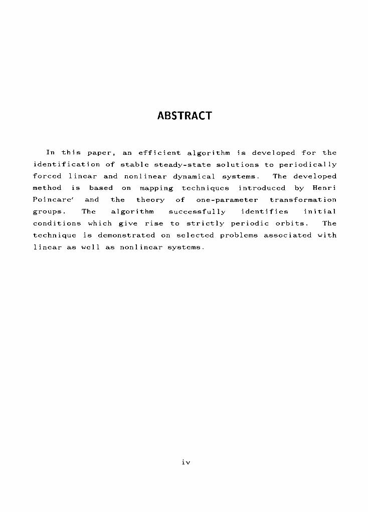
ABSTRACT

In this paper, an efficient algorithm is developed for the

identification of stable steady-state solutions to periodically

forced linear and nonlinear dynamical systems. The developed

method is based on mapping techniques introduced by Henri

Poincare'and the theory of one-parameter transformation

groups. The algorithm successfully identifies initial

conditions which give rise to strictly periodic orbits. The

technique is demonstrated on selected problems associated with

linear as well as nonlinear systems.

IV

TABLE OF CONTENTS

Page

Acknowledgements iii

Abstract iv

List of Figures vi

L i st of Symbo Is viii

I INTRODUCTION 1

II DYNAMICAL SYSTEMS 17

A. Dynamical Systems 17

B. Poincare'

Mapping 28

III LINEAR SYSTEMS 32

A. Fundamental Solutions/Fundamental Matrix 34

B. Fundamental Matrix 36

C. Forced Solutions 40

D . 1 -D Systems 42

Higher Dimensional Systems 61

IV NONLINEAR SYSTEMS 88

A. Infinitesimal Generators 89

B.Poincare'

Map Development 94

C. Nonlinear Algorithm 98

D. 1-D Nonlinear Systems 100

Higher Dimensional Systems 115

V CONCLUSIONS AND RECOMMENDATIONS 131

REFERENCES 133

APPENDICES 134

v

LIST OF FIGURES

Figure Page

1-1 Phase space 7

1-2 Phase curves 8

1-3 Reduced phase space/state space 8

1-4 Phase flow 9

1-5 Integral curces defining a phase flow 10

1-6 Integration of integral curves 11

1-7 Projection operators showing mapping onR"

12

1-8 Mapping of P in the state space 12

1-9 Integral curve motion at different values of the

forcing period 13

1-10 Image of a single forcing period 14

2-1 Mass-Spring-Damper system 17

2-2 Real 1 ine 19

2-3 Periodic forcing functions 20

2-4 1 -D state space 23

2-5 1-D state space 24

2-6 2-D state space 25

2-7 Phase space 28

2-8 Phase space plot ofPoincare'

mapped point 30

3-1 Mass-spring-damper system 32

3-2 Block diagram representation of excitation

and response of a system 33

3-3 State space: R,the real line 42

3-4Poincare'

mapping of state values 43

3-5Poincare'

mapping of a fixed initial pointx*

from t= 0 to t=T 45

vi

LIST OF FIGURES (continued)

Figure Page

4-1 System input and response recorded side by side

while seeking the system periodic solution 93

4-2 Mapping of point x from t=t0 to t=T 94

4-3 Forward advance mapping of x to the eventual

Poincare'

mapping of x 95

4-4 Forward advance mapping and thePoincare'

mapping

of point and sequence of points 96

4-5 Forward advance mapping scheme 103

LIST OF SYMBOLS

A,B,C Constant

A< Time dependent operator

[A] , [B] , [K] . . . .Square matrix

[I] Identity square matrix

c Viscous damping constant

F Force function

F Force vector

f Periodic input function

f Periodic forcing vector

G Forward advance transformation

G'Derivative of G for 1-D system

DG Partial derivative of G

J Jacobian operator

JG Jacobian of G function

JP Jacobian of P function

H System chracter ist ic Transfer function

x,y Rectangular coordinates, distances

x,y Time derivative of coordinates, x,y

x Time derivative of x

x0,y0 Initial conditions for x,y

x*

Initial value that gives periodic solution, x0

x,y Position vector

g(x) ,y(x) Vector functions

xh

Series solution expansion

k Spring stiffness constant

m Mass

M Manifold, n-d imens ional

N Number of time interval

P Poincare map

P' Derivative of Poincare Map for 1-D system

DP Partial derivative of P

v 1 1 1

LIST OF SYMBOLS (continued)

R Real space

T Period

t Time

t0 Initial condition of t

t Period: Periodic time

<P Forward advance transformation function

#o Trajectory at time t0

$t Trajectory at time"t"

#T Trajectory at time t = T (period)

^nT Trajectory at time t = nT

w Circular frequency of forced vibration

Un Natural frequency

Q Driving frequency of system

t Small element, accuracy error parameter

j3 System parameter constant

Viscous damping factor

U Infinitesimal Generator operator

v Velocity

v Acceleration

x'1

Series solution

{x(t)} Displacement vector

{y(t) } State vector

{F(t) } Force vector

{x(t)} Velocity vector

u(t) Forcing vector

JL Partial derivetive operator w.r.t x

dx

TJ Mapping

IX

INTRODUCTION

Oscillatory motion is an important aspect in the fields of

physics and engineering. Periodic motion is common in most

physical systems. Some examples include the motion of planets,

the earth around the sun, the moon around the earth, the

movement of bodies of water (ocean waves) , all repeating their

motion after a specified time. The analysis of oscillations is

an important part of mechanical vibration, and is an essential

design criterion that is necessary in almost all structural and

mechanical systems in present day engineering design.

Any attempt to design a mechanical system usually begins

with a prediction of its performance. Linear vibration analysis

has been adequate for most applications. However, because of

the current high demand for greater system performance, the

application of linear analysis sometimes results in failures.

Many of these failures are a result of nonlinear effects in

systems that were designed under the assumption of linear

behavior. Nonlinear analysis now receives considerable

attention in an effort to understand phenomena not predicted by

traditional linear analysis.

Physical systems are modeled by differential equations.

Based on the nature of the differential equation, the system

can be classified as linear or nonlinear- There are many

characteristics which distinguish between the solutions of

linear and nonlinear differential equations. For example, the

fundamental system of solutions exists only for linear

differential equations [1] This implies that if certain basic

solutions are known, the general solution will be a linear

combination of these fundamental solutions. However, it is more

often than not impossible to analytically solve nonlinear

differential equations. Consequently, because of the difficulty

involved, approximation methods and qualitative analyses of the

solutions become important in studying the nature of nonlinear

oscillations [2] .

Linear analysis is a rather mature subject. It is a

unified theory based on concepts and results from linear

algebra and its generalization, functional analysis. The

principle of superposition allows linear differential equations

to be solved analytically. All solutions can be constructed

from the fundamental solutions which are exponential functions

[2,14] . This limits the type of behavior encountered in linear

systems. Its utility in solving a vast multitude of physical

problems, however, remains unsurpassed.

The analysis of nonlinear systems is a richer topic in

comparison to the standard linear theory. The lack of a unified

theory that would encompass nonlinear analysis allows for

considerable variation in system properties and qualitative

behavior. Not only do nonlinear systems behave differently from

linear ones, the system response may at first seem unintuitive.

Limit cycles, for example, are unique to some dissipative

nonlinear systems. Limit cycles are isolated periodic solutions

which attract a dense subset of the state space [6] . Other

phenomena include amplitude instabilities, catastrophes and

chaotic behavior [1,6].

The focus of this investigation is the steady state

behavior of linear and nonlinear systems. Steady state behavior

is understood to be the long-term response of a system due to

external forcing. The attention will be restricted to periodic

behavior, which occurs universally in linear as well as

nonlinear systems. In particular, a general method for the

determination of period solutions will be proposed and

examined. The proposed method is constructive, that is, it

yields actual results. In addition, the idea is applicable to

linear and nonlinear systems without modification.

Some attention has been focused on the determination of

steady state solutions [3-6] . Typical methods of analysis for

steady state periodic response (for a given initial state x0 at

time t0) entail integrating the governing matrix equations

until the response becomes periodic. This means that the

transient response becomes negligible. For lightly-damped

systems the analysis is exceedingly slow, and could be

prohibitive, as it must extend over far too many periods. Also,

it is hard to tell whether a stable orbit exists and what its

period T is, or whether or not the response will end up at a

singular point. This method is called the brute-force approach.

Aprille and Trick [3] developed a series of algorithms for

the determination of periodic solutions associated with

problems in nonlinear circuit analysis. Their proposed method

was apparently successful, but the outlined procedure is

cumbersome. It requires integration of the system equations

together with the coupled variational equations. The

variational equations constitute a linearization of the system

about a specified solution. Hence, n+1 analyses are required

for each iterate where n is the dimension of the state space.

A more systematic approach has been developed, one that

rapidly determines initial conditions which give rise to

strictly periodic solutions. The methodology has been automated

by the use of a symbolic computation program, MAPLE. This

generalized approach is briefly outlined below.

The integration of the system equations up to a fixed time

defines a family of point transformations, parameterized by the

time variable, mapping the state space into itself. The method

of solution requires the use of Lie group theory. This allows

the construction of the global transformation equations with

the characteristic infinitesimal generator of the group [11] .

The solutions generated by such a Lie series representation

constitute a generalization of solutions obtained for linear,

constant coefficient systems [14] . Recall that the fundamental

matrix solution is expressible as a series expansion of a

matrix-valued exponential function. The primary motivation for

developing Lie series solutions to differential equations is

that complete solutions to the problem are generated for

arbitrary initial conditions. With the availability of

computational and symbolic mathematics programs [9] ,the series

solution of differential equations are much more feasible now

[11].

BACKGROUND

There are two kinds of dynamical systems that are

encountered in vibration analysis, autonomous systems and

forced systems which are called nonautonomous . For a

nonautonomous system, the independent variable t (time) is

present in the forcing function of the system differential

equation. The function depends explicitly on t. The first order

system given below is nonautonomus :

x = f(x,t) (1.1)

On the other hand, autonomous system differential equations

have no explicit dependence on t. The differential equation in

(1.2) is an example of an autonomous first order system:

x = f(x,y) (1.2)

y = g(x,y)

In this investigation we will propose a general method to find

periodic solutions of nonautonomous system equations. Although

the methodology is completely general, the discussion will

focus separately on first-order systems, higher-order systems,

linear and nonlinear systems.

Nonautonomous Systems

Consider the nonautonomous first-order equation

x = f(x,t) (1.3)

where f is periodic in t of period T, and is continuous in t

and x. The analysis of periodic solutions is a nontrivial

problem. It is essentially a two-point boundary value problem

in which the solution to (1.3) on the interval [0,T] must

satisfy the boundary condition

x(0) = x(T) (1.4)

This type of problem can be solved using the shooting method

for boundary value problems. But this technique would be

cumbersome at best. Integrating both sides of equation (1.3)

x(T) = f (x,r)dr + x(0) (1.5)

o

We can express the above problem in terms of a mapping

x0 = V(x0) (1.6)

where

x0= x(0) (1

.6a)

T

V(x0)= I "f(x, r) dr + x0 (1.6b)

o

and x(t)satisfies equation (1.3) for 0 < t < T.

One approach to finding the periodic solution of equation

(1.6) is by means of the Newton Raphson iteration

x0 = - [I -

d^(x</)][x0'

-

v(x0')] (1.7)

where

dv(x0) =

,._ dx(T;x0)

3xn(1.8)

We will review the concept of aPoincare'

Mapping and in

the process show how to use it for finding periodic solutions

of nonautonomous systems .

Poincare'

Mapping for Nonautonomous Systems

Consider the nonautonomous system

x = f(x,t) x R", fCx(RxR"

R") (1.9)

With a simple association of variables 9 =

t, we convert to the

autonomous system

x = f(x,0)

(9 = 1

vector field onn+ l

(1.10)

Hence any general results for autonomous systems onRm

,m > 2

will hold for nonautonomous systems as well.

Of particular (and practical) interest is when f(x,t) is

periodic in t. That is,

f(x,t) = f(x,t + T) (1.11)

for each fixed x. In any case, the phase space for the system

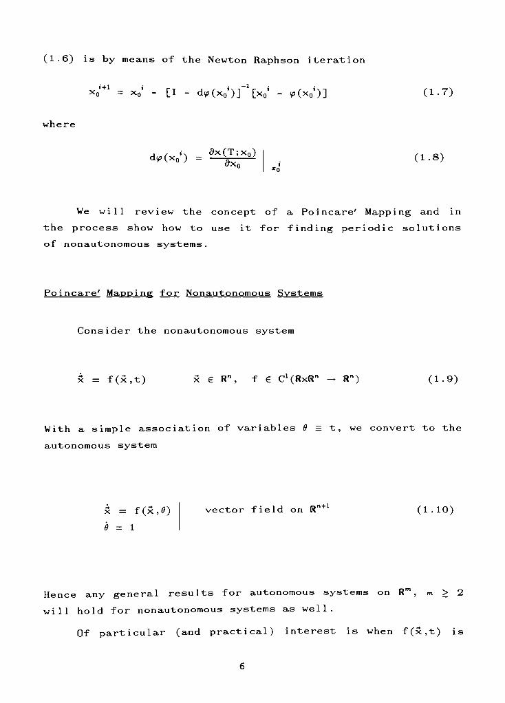
in equation (1.9) is n+i dimensional:

R"

FIG 1-1. Phase space

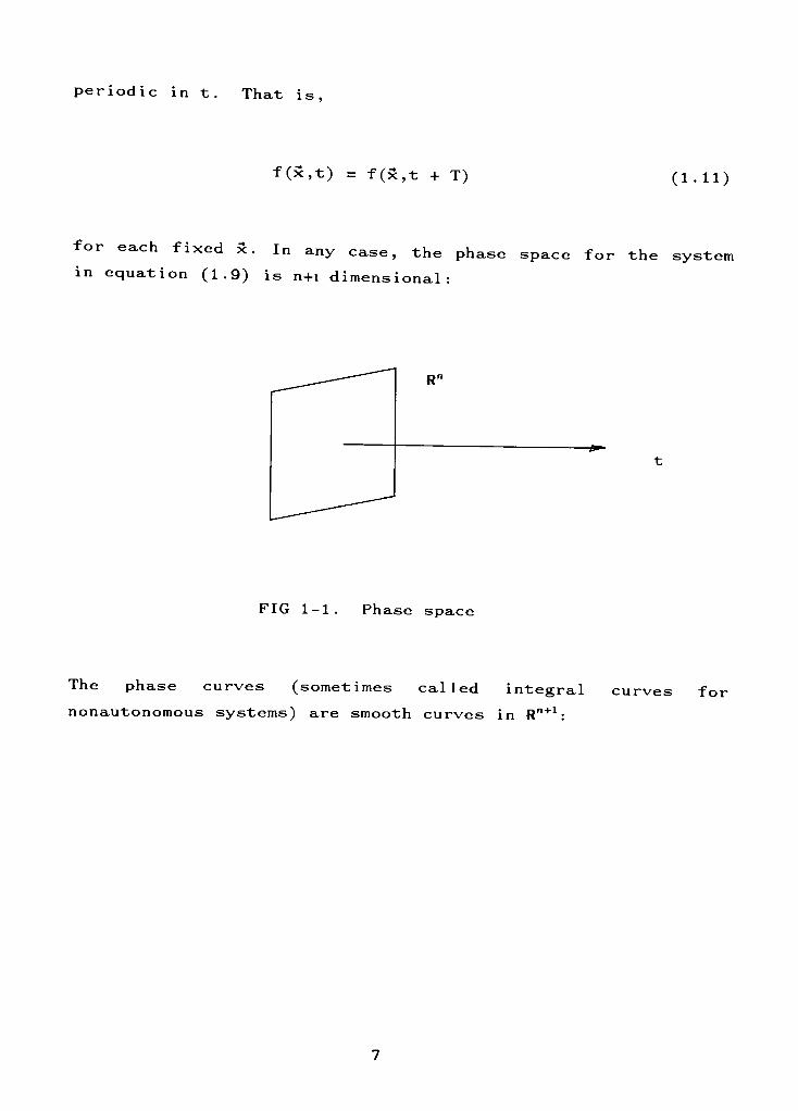
The phase curves (sometimes called integral curves for

nonautonomous systems) are smooth curves inR"+1

:

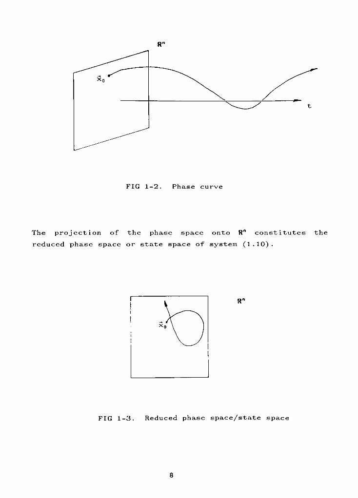
FIG 1-2 Phase curve

The projection of the phase space ontoRn

constitutes the

reduced phase space or state space of system (1.10) .

R"

FIG 1-3. Reduced phase space/state space

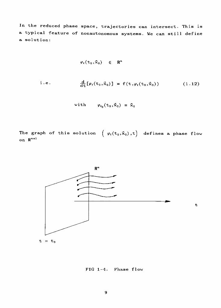
In the reduced phase space, trajectories can intersect. This is

a typical feature of nonautonomous systems. We can still define

a solution:

(P(t0,x0)R"

1 . e ^LV(*o.x0)] = f (t,Y?t(t0,x0)) (1.12)

with V0(t0,x0) =x0

The graph of this solution ( p (t0 ,x0) ,t J defines a phase flow

onRn+1

Rn

t = tr

FIG 1-4. Phase flow

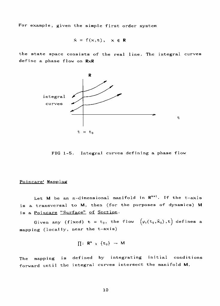
For example, given the simple first order system

x = f (x,t) , x G R

the state space consists of the real line. The integral curves

define a phase flow on RxR

R

integral

curves

t = tr

FIG 1-5. Integral curves defining a phase flow

Poincare' Mapping

n+ 1

Let M be an n-d imens ional manifold in R .If the t-axis

is a transversal to M, then (for the purposes of dynamics) M

is a Poincare"Surface"

of Section .

Given any (fixed) t = t0 ,the flow (v?t (t0 ,x0) , tj

defines a

mapping (locally, near the t-axis)

n=R"

x {t0} M

The mapping is defined by integrating initial conditions

forward until the integral curves intersect the manifold M .

10

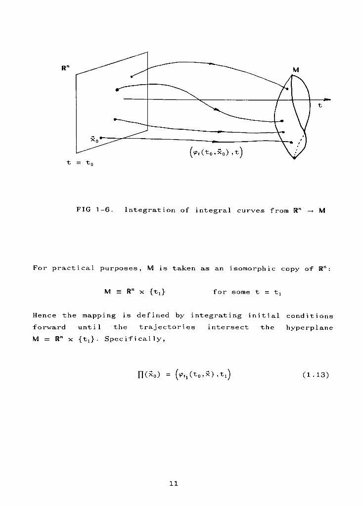
t = tf

FIG 1-6. Integration of integral curves fromR"

< M

For practical purposes, M is taken as an isomorphic copy ofRn

:

M =R"

x {tj for some t = tx

Hence the mapping is defined by integrating initial conditions

forward until the trajectories intersect the hyperplane

M =R"

x {tj}. Specifically,

n(xo) = (^(to.x),tx) (1.13)

11

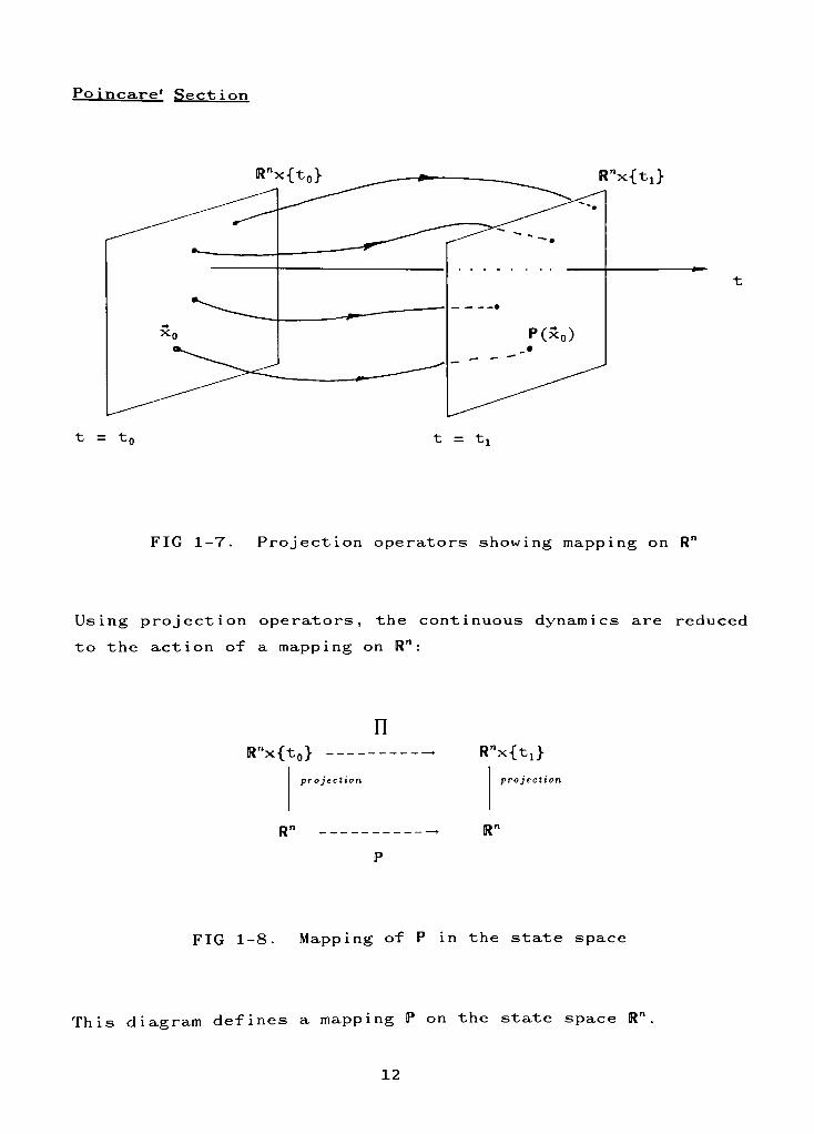
Poincare'Section

Rnx{t0} R"x{tJ

t = tfl t = t.

FIG 1-7. Projection operators showing mapping onR"

Using projection operators, the continuous dynamics are reduced

to the action of a mapping onR"

:

n

Rnx{t0}

projection

Rn

Rnx{t1}

projection

p

FIG 1-8. Mapping of P in the state space

This diagram defines a mapping P on the state spaceRr

12

": R ?Rn

can also be considered as a forward -advance

mapp ing.

Letting now the initial condition be arbitrary (dropping

the subscript)

P(x) =^(t0,x) (1.14)

[ note that the"initial"

time and final have been fixed ]

The Poincare'

Mapping (corresponding to a Euclidean surface of

section) reduces the investigation of the dynamics to the

analysis of n-dimens ional maps. The following observations can

be made :

The behavior of the flow is preserved by the mapping.

That is, convergence or divergence of trajectories can

be investigated.

The"dimension"

of the problem is effectively reduced

by one .

ThePoincare'

Mapping is most useful in studying periodic

solutions, limit sets, and asymptotic behavior. This paper will

focus on its use in the investigation of periodic solutions.

Periodic Solutions

Consider x = f(t,x) (on R")

with f(t + T,x) = f(t,x) for each x GR"

We can convert to an equivalent autonomous system (using 0 =wt)

x =(f(5,x)

0 = u where u = 4S-

13

Now f(,x) is 2ir-periodic in 0.

To investigate the periodic solutions, the integral curves are

"tracked"at multiples of the forcing period

R"x{<?0}

0 = 0

FIG 1-9. Integral curve motion at different values of 9

But since the forcing function f(^,x) is 2?r-per iod ic, we need

to concentrate only on the single forcing period 90 < 9 < 90 +

"2ir and keep track of the images:

0 = 9, 0 = 90 + 2ir

FIG 1-10. Image of a single forcing period

14

That is we re-start the dynamics with a"new"

initial condition

each time. The integral curves (solutions) are effectively

tracked by deducing the Poincare'

Mapping

P: RnR"

[Each point is integrated forward over the interval 0 to 0o+2jt]

Theorem: Given x = f(t,x) inRn

, f(t,x) T periodic. The

system has a T-periodic solution if the associatedPoincare'

Mapping, P, has a fixed point Xn.

Proof: Clearly, a T-periodic solution results in a fixed point

of thePoincare'

Mapping. Suppose P(xp) =

xp for some XpR"

.

This means that

^T+t (tD'^p)=

*Pfor t,he solution Vt(t0,xp).

But ^[ ?T+((t0,xp)]= f(t+T, ^T+((t0,xp))

= f(t, VT+t(to,xp))

Hence ^t(t0,xp) andip^ t(t0,xp)

are two solutions with the same

initial condition xp. By uniqueness of solutions,

Vt(t0,xp)= v?T+((t0,xp)

Since the continuous dynamics is reduced to the action of a

mapping, the rich collection of f ixed-point theorems can be

utilized to investigate periodic solutions.

This paper will show an efficient technique developed,

based on the theory ofPoincare'

Mapping, that identifies

initial conditions associated with periodic solutions for

forced linear and nonlinear dynamic systems.

15

The algorithm developed for locating periodic solutions to

linear and nonlinear systems will be reviewed. The process uses

modifications to the method of analysis for determining steady

state periodic response, with techniques ofPoincare'

Mapping

[4] and the Infinitesimal Generator associated with Lie Series

[8,11] . The. main part of the review is outlined in two

chapters. Chapter three starts with one dimensional (1-D)

linear system analysis and extends the analysis for higher

dimension linear systems. Chapter four discusses the analysis

of I-D nonlinear systems and continues on to the analysis of

higher dimension nonlinear systems.

The use of the symbolic computation mathematics program

Maple, will be used for its speed in calculating solutions for

differential equations and the generation of series solution

expansions. Discussions on how the algorithm is applied and

examples will be reviewed.

16

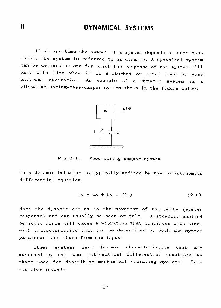
II DYNAMICAL SYSTEMS

If at any time the output of a system depends on some past

input, the system is referred to as dynamic. A dynamical system

can be defined as one for which the response of the system will

vary with time when it is disturbed or acted upon by some

external excitation. An example of a dynamic system is a

vibrating spring-mass-damper system shown in the figure below.

F(t)

/ / / / / / / / /

FIG 2-1. Mass-spring-damper system

This dynamic behavior is typically defined by the nonautonomous

differential equation

mx + ex + kx = F(t) (2.0)

Here the dynamic action is the movement of the parts (system

response) and can usually be seen or felt. A steadily applied

periodic force will cause a vibration that continues with time,

with characteristics that can be determined by both the system

parameters and those from the input.

Other systems have dynamic characteristics that are

governed by the same mathematical differential equations as

those used for describing mechanical vibrating systems. Some

examples include:

17

1. Electrical circuits, composed of resistive, capacitive and

inductive elements that will oscillate (fluctuate) under

the proper type of excitation.

2. Ecological systems. The population of a species of insects

or mammals in a given region can vary from year to year

because of factors such as the number of predators (and the

interaction between predators and prey), disease, weather

conditions and food supply.

3. Flow of traffic. Different types of traffic disturbances

can result in dynamic characteristic behavior of human

beings behind the wheel which can be modeled by

differential equations.

The type of information that one wants to know about a

dynamic system is essentially the same regardless of the

physical details of the system. It is important to know :

1. How the system responds with time for any particular type

of disturbance.

2. How long it will take for the dynamic action to dissipate

if the disturbance is applied only briefly and then removed

3. Whether the system is stable or if its oscillations will

increase in magnitude with time after the disturbance has

been removed .

The objective of this investigation is to examine the

steady state behavior of linear and nonlinear dynamical

systems. The concept ofPoincare'

Mapping in conjunction with

forward advance transformation, will be used to show the

effectiveness of the method developed for seeking periodic

solutions of these systems.

18

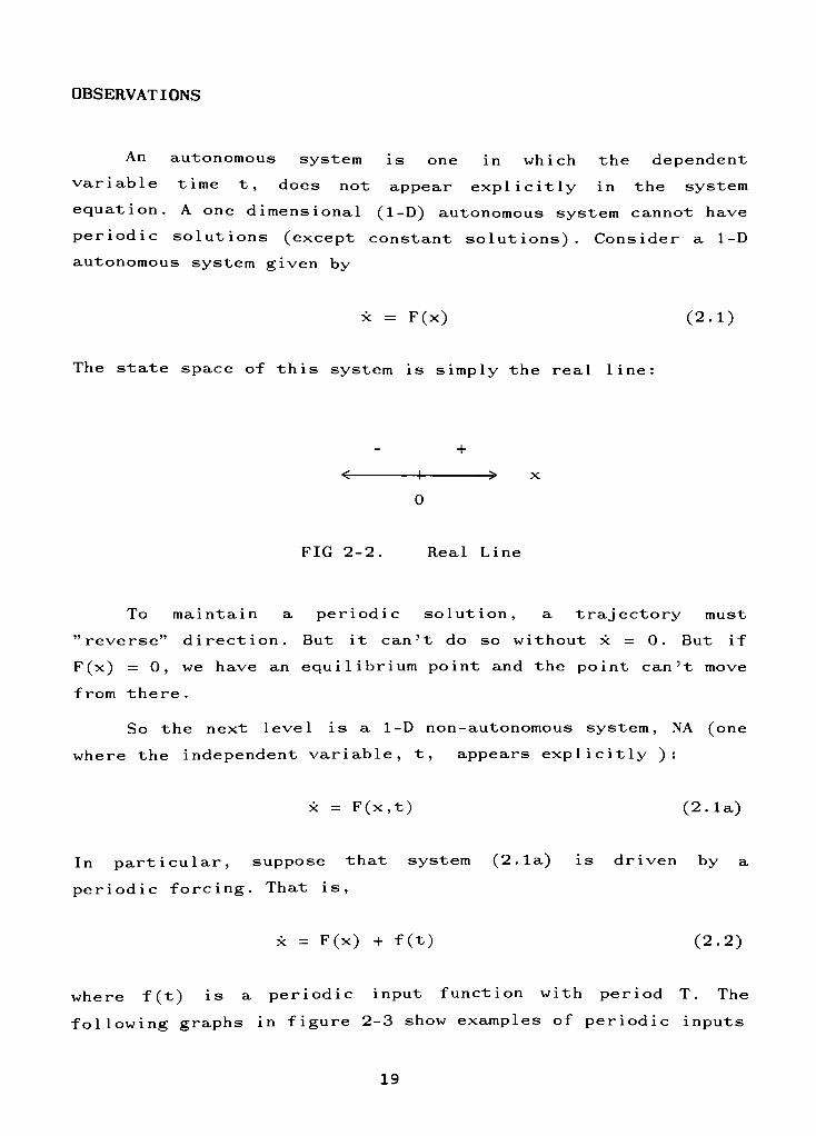
OBSERVATIONS

An autonomous system is one in which the dependent

variable time t, does not appear explicitly in the system

equation. A one dimensional (1-D) autonomous system cannot have

periodic solutions (except constant solutions). Consider a 1-D

autonomous system given by

x = F(x) (2.1)

The state space of this system is simply the real line:

+

>

0

FIG 2-2. Real Line

To maintain a periodic solution, a trajectory must

"reverse"

direction. But it can't do so without x = 0. But if

F(x) = 0, we have an equilibrium point and the point can't move

from there .

So the next level is a 1-D non-autonomous system, NA (one

where the independent variable, t, appears explicitly ):

x = F(x,t) (2.1a)

In particular, suppose that system (2.1a) is driven by a

periodic forcing. That is,

x = F(x) + f(t) (2.2)

where f(t) is a periodic input function with period T. The

following graphs in figure 2-3 show examples of periodic inputs

19

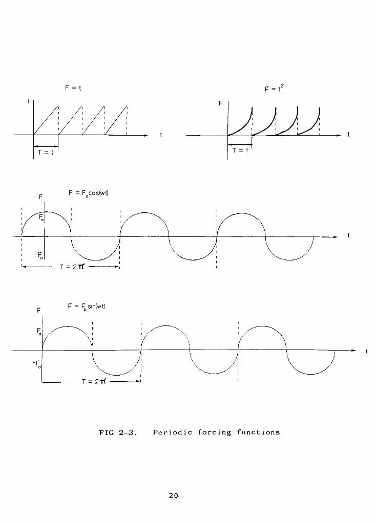
F = t F =

t'

t

F = F cos(wt)

0

i

^^ ii i

i

/~

^"~\ i

i / \ i /

'/ \ '/

-F

'^ T = 2Tf -

i

F =

FQ sin(wt)

T = 2"K

FIG 2-3. Periodic forcing functions

20

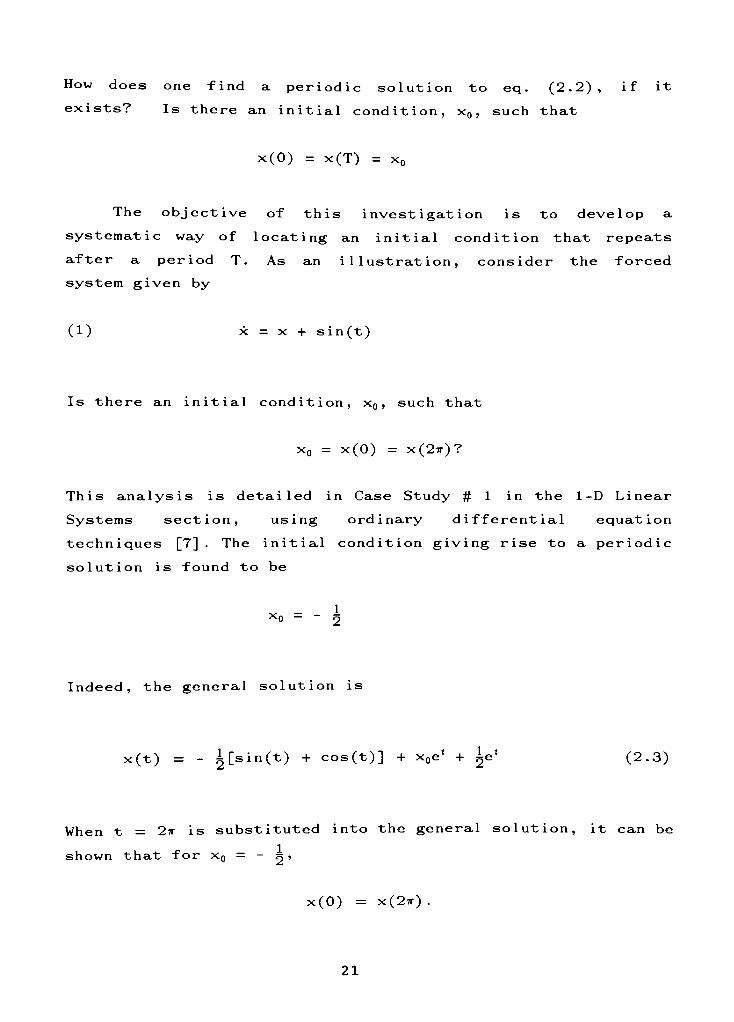
How does one find a periodic solution to eq. (2.2), if it

exists? Is there an initial condition, x0 ,such that

x(0) =x(T) = x0

The objective of this investigation is to develop a

systematic way of locating an initial condition that repeats

after a period T. As an illustration, consider the forced

system given by

(1) x = x + sin(t)

Is there an initial condition, x0 ,such that

x0 = x(0) = x(2:r)?

This analysis is detailed in Case Study # 1 in the 1-D Linear

Systems section, using ordinary differential equation

techniques [7] . The initial condition giving rise to a periodic

solution is found to be

x-

- 1x0 -

-

2

Indeed, the general solution is

:(t)= - i[sin(t) + cos(t)] +

x0e'

+le*

(2.3)

When t = 2ir is substituted into the general solution, it can be

shown that for x0= -

7y >

x(0)= x(2t) .

21

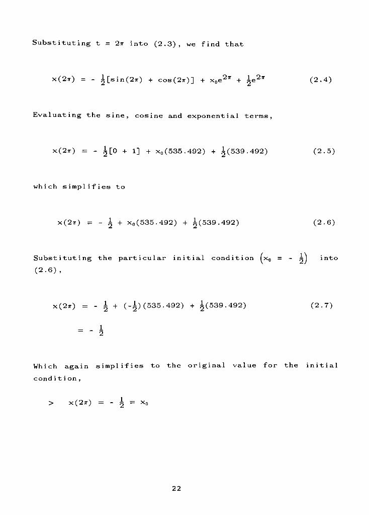
Substituting t = 2ir into (2.3), we find that

x(2tt) = - l[sin(2x) + cos(2i)] +x0e2,r

+ie2*

(2.4)

Evaluating the sine, cosine and exponential terms,

x(2t) = - i[0 + 1] + x0(535.492) + i(539.492) (2.5)

which simplifies to

x(2tt) = - + x0(535.492) + (539.492) (2.6)

Substituting the particular initial condition lx0 = - i] into

(2.6),

x(2tt)= - i + (-1) (535.492) + i(539.492) (2.7)

_

_

1~

2

Which again simplifies to the original value for the initial

condit ion ,

> x(2?r)= - i = x0

22

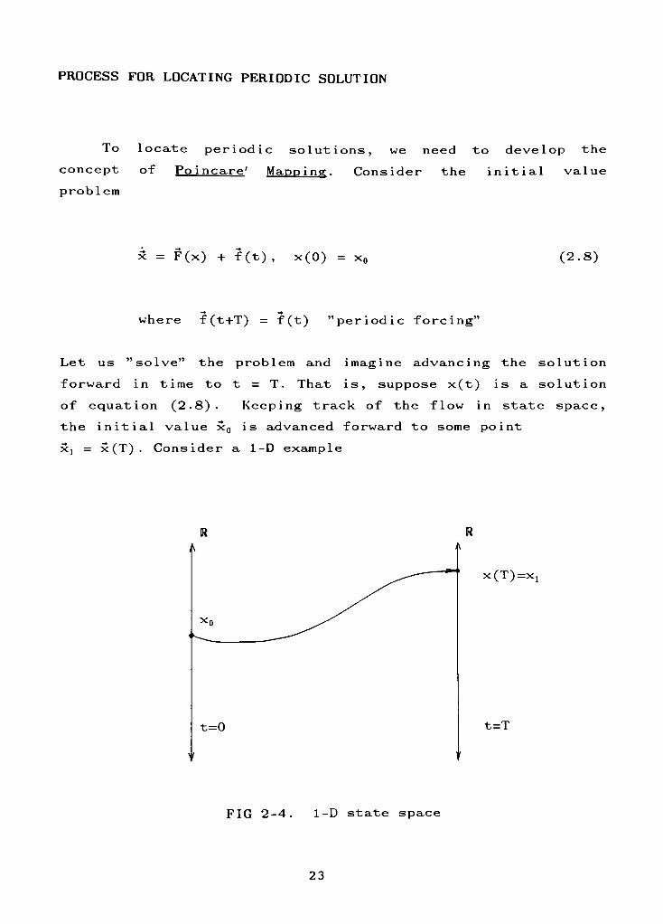
PROCESS FOR LOCATING PERIODIC SOLUTION

To locate periodic solutions, we need to develop the

concept ofPoincare'

Mapping. Consider the initial value

problem

x = F(x) + f (tO, x(0) =x0 (2.8)

where f(t+T) = f (t) "periodicforcing"

Let us"solve"

the problem and imagine advancing the solution

forward in time to t = T. That is, suppose x(t) is a solution

of equation (2.8) . Keeping track of the flow in state space,

the initial value x0 is advanced forward to some point

xx= x(T) . Consider a 1-D example

x(T)=Xl

t=T

FIG 2-4. 1-D state space

23

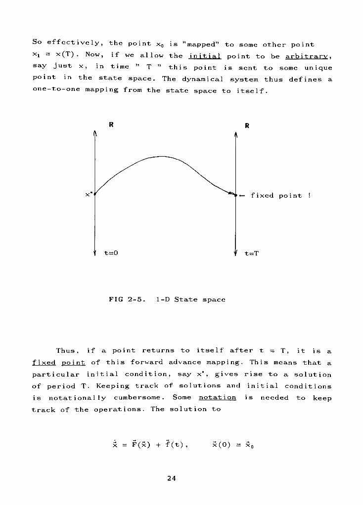
So effectively, the point x0 is "mapped"to some other point

xi =X(T) Now, if we allow the initial point to be arbitrary.

say just x, in time"

T"

this point is sent to some unique

point in the state space. The dynamical system thus defines a

one-to-one mapping from the state space to itself.

R

fixed point !

"' t=T

FIG 2-5. 1-D State space

Thus, if a point returns to itself after t = T, it is a

f ixed po i nt of this forward advance mapping. This means that a

particular initial condition, sayx*

,gives rise to a solution

of period T. Keeping track of solutions and initial conditions

is notationally cumbersome. Some notat i on is needed to keep

track of the operations. The solution to

x = F(x) + f(t), x(0) =x0

24

is denoted by

*t(x0) = solution trajectory at time"t"

, (2.9)

starting at x0 !

We can denote the solution for arbitrary initial conditions by

dropping the subscript. So #t = solution of the Initial Value

Problem (IVP), starting at x, #(x). i.e.

^[*,(x)] =

F(#t(x)) + f(t) (2.10)

with $0(x) = x

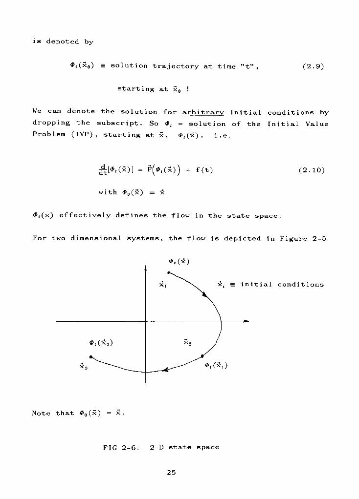
#t(x) effectively defines the flow in the state space

For two dimensional systems, the flow is depicted in Figure 2-5

*-(x)

x,= initial condit:

*.(xi)

Note that #0(x) = x

FIG 2-6. 2-D state space

25

$(x) describes the evolution of each point in the state space.

Thus, #<(x) is the forward advance mapping (at time "t")

starting at x. This allows us to express with a single symbol a

solution in time, starting at an arbitrary point x.

Examples :

(1) x = x general solution: x(t) =Ae1

.

Now x(0) = A, so the forward advance map is

*t(x)=xe'

(2.11)

It is important to keep in mind that now'x'

represents an

arbitrary initial condition.

(2) x = -x + t general solution: x(t) = t-1 + Ce'

x(0) = -1 + C

=> C = x(0) + 1

Eliminating the constant of integration results in the general

solution

x(t)= t - 1 + (x0 +

l)e-'

Letting the initial condition be arbitrary, the forward advance

mapping is explicitly given by

4>((x) = t - 1 +(x+l)e_(

(2.12)

That is, after a time t any initial value x G R gets mapped to

(t-1) +(x+l)e-(

26

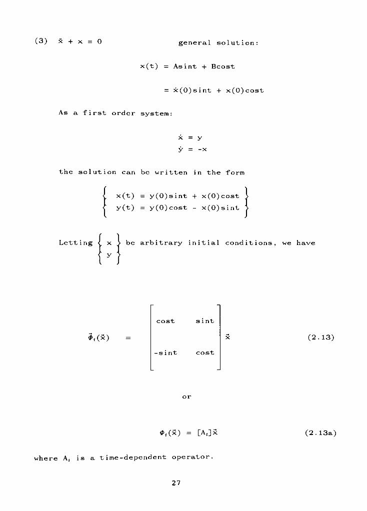
(3) x + x = 0 general solution

x(t) = Asint + Bcost

= x(0)sint + x(0)cost

As a first order system :

x = y

y = -x

the solution can be written in the fo rm

x(t) = y(0)sint + x(0)cost

y(t) = y(0)cost - x(0)sint

Letting {, x j be arbitrary initial conditions, we have

y

*(x)

cost s i nt

-sint cost

(2.13)

or

*(x) = [At]x (2.13a)

/here At is a time-dependent operator.

27

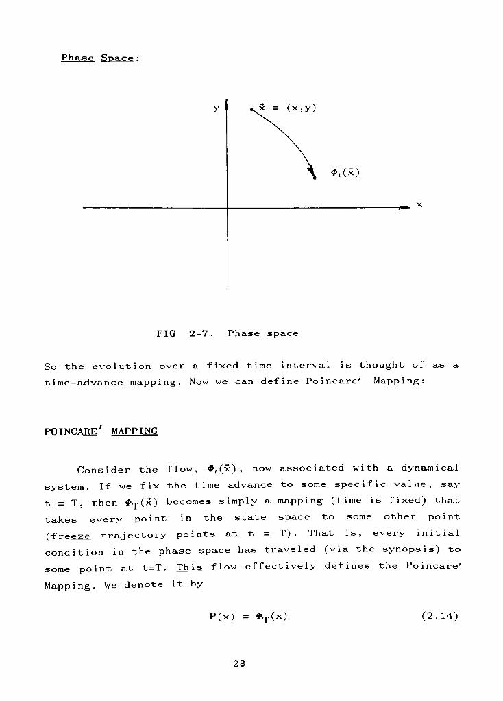
Phase Space :

y I, 5c = (x,y)

*.(*)

FIG 2-7. Phase space

So the evolution over a fixed time interval is thought of as a

time-advance mapping. Now we can definePoincare' Mapping:

poincare'

mapping

Consider the flow, $<(x), now associated with a dynamical

system. If we fix the time advance to some specific value, say

t = T, then #T(x) becomes simply a mapping (time is fixed) that

takes every point in the state space to some other point

(freeze trajectory points at t = T) . That is, every initial

condition in the phase space has traveled (via the synopsis) to

some point at t=T . This flow effectively defines thePoincare'

Mapping. We denote it by

P(x) = *T(x) (2.14)

28

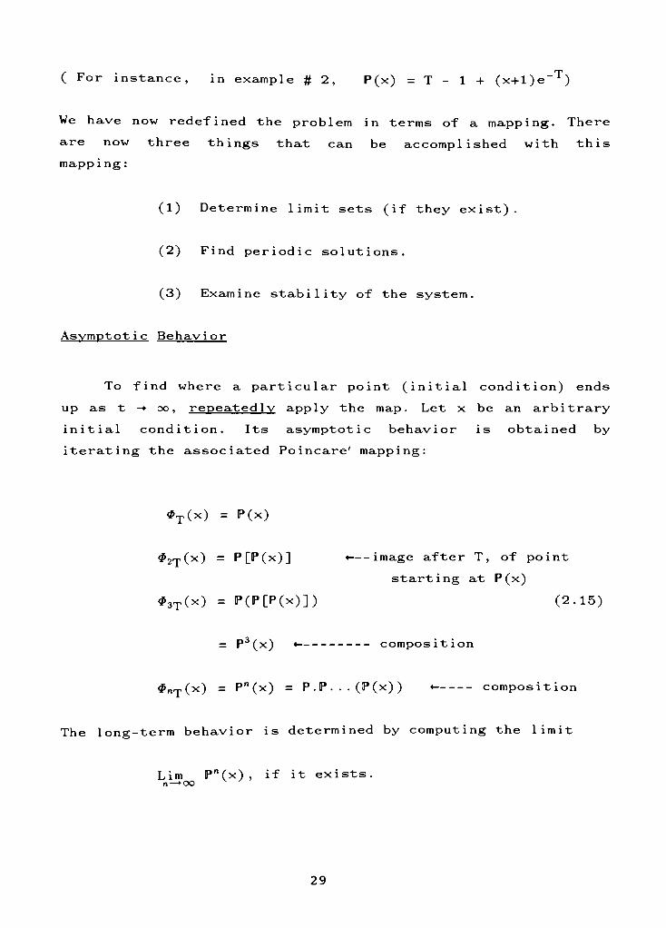
( For instance, in example # 2, P(x) = T - 1 + (x+l)e"T)

We have now redefined the problem in terms of a mapping. There

are now three things that can be accomplished with this

mapping :

(1) Determine limit sets (if they exist).

(2) Find periodic solutions.

(3) Examine stability of the system.

Asvmptot i c Behavi or

To find where a particular point (initial condition) ends

up as t - oo, repeatedly apply the map. Let x be an arbitrary

initial condition. Its asymptotic behavior is obtained by

iterating the associatedPoincare'

mapping:

#T(x) = P(x)

#2ry,(x) = P[P(x)] < image after T, of point

starting at P(x)

43T(x) = P(P[P(x)]) (2.15)

= P3(x) composition

<pT(x)= P"(x) = P.P...(P(x)) < composition

The long-term behavior is determined by computing the limit

Lim P"(x), if it exists.n >00

29

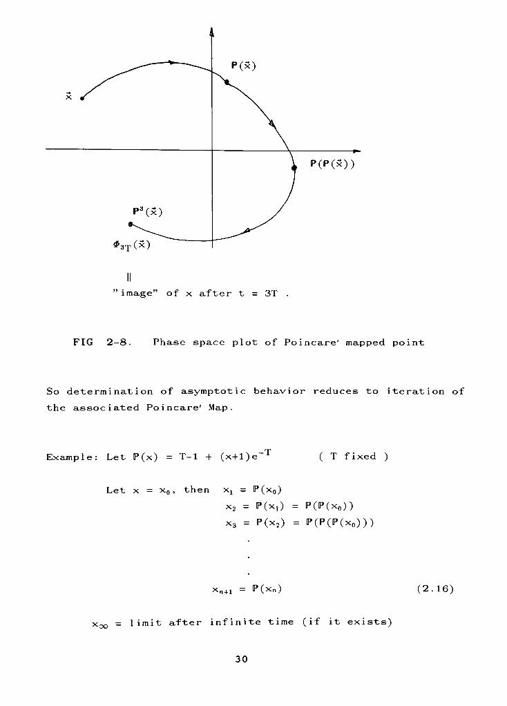
image"of x after t = 3T .

FIG 2-8. Phase space plot ofPoincare'

mapped point

So determination of asymptotic behavior reduces to iteration of

the associatedPoincare'

Map.

-T

Example: Let P(x) = T-1 + (x+l)el

( T fixed )

Let x = x0, then xx= P(x0)

x2= P(xx)

x3= P(x2)

P(P(x0))

P(P(P(x0)))

xn+i= P(x) (2.16)

^oo= limit after infinite time (if it exists)

30

Example: Find the limit of any solution to

x = -x + t (period T = 1)

The initial condition giving rise to a periodic limit solution

was found to be

x0 = 0.582

In fact, all initial conditions converge to this value in the

limit. See Chapter III, 1-D Linear Systems, Case Study 2 for

problem detail .

Period i c Solut i ons

The main focus of this investigation is the determination

of periodic solutions (if they exist). Periodic means that the

solution repeats itself. This requires finding a f ixed do int of

thePoincare' Map. Thus

x*

gives rise to a periodic solution if

x*

= P(x*) = <?T(x*) (2.17)

i.e, after time T,x*

returns tox*

ThePoincare' Mapping is the tool we will use to locate

periodic solutions. If the Poincare mapping can be constructed,

these periodic solutions are readily computed. In most cases,

however, thePoincare'

mapping must be approximated. This

important aspect will be discussed in the subsequent chapters.

31

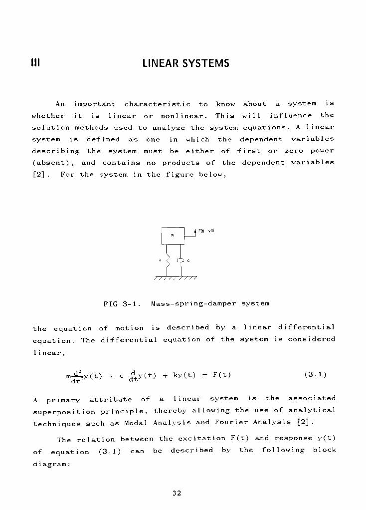
Ill LINEAR SYSTEMS

An important characteristic to know about a system is

whether it is linear or nonlinear. This will influence the

solution methods used to analyze the system equations. A linear

system is defined as one in which the dependent variables

describing the system must be either of first or zero power

(absent) ,and contains no products of the dependent variables

[2] . For the system in the figure below,

Fit) y(t)

/////////

FIG 3-1. Mass-spring-damper system

the equation of motion is described by a linear differential

equation. The differential equation of the system is considered

1 inear ,

mfiy(t) + c ^y(t) + ky(t) = F(t)dtJ

(3.1)

A primary attribute of a linear system is the associated

superposition principle, thereby allowing the use of analytical

techniques such as Modal Analysis and Fourier Analysis [2] .

The relation between the excitation F(t) and response y(t)

of equation (3.1) can be described by the following block

d i agram :

32

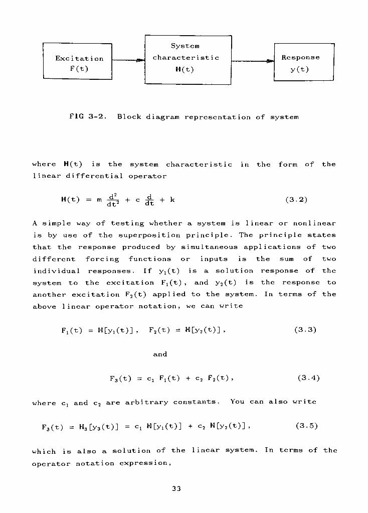
System

characteristic

H(t)

Excitat ion

F(t)

&Response

yOO

FIG 3-2. Block diagram representation of system

where H(t) is the system characteristic in the form of the

linear differential operator

H(t) = m } + c A + kdt (3.2)

A simple way of testing whether a system is linear or nonlinear

is by use of the superposition principle. The principle states

that the response produced by simultaneous applications of two

different forcing functions or inputs is the sum of two

individual responses. If yi(t) is a solution response of the

system to the excitation Fx(t), and y2(t) is the response to

another excitation F2(t) applied to the system. In terms of the

above linear operator notation, we can write

FiOO = H[yi(t)], F2(t) = H[y2(t)], (3.3)

and

F3(t) = cx Fx(t) + c2 F2(t) , (3.4)

/here cl and c2 are arbitrary constants. You can also write

F300 [y3(-t)l = cx H[Yl(t)] + c2 H[y2(t)], (3.5)

which is also a solution of the linear system. In terms of the

operator notation expression,

33

H[ciyi + c2y2] =Cl H[Yl] + c2 H[y2] (3.6)

represents the statement that the operator H is linear,

implying that the superposition principle holds true for the

system whose characteristics are described by H. If on the

other hand,

FsOO = H3[y3(t)] Cl H[Yl(t)] + c2 H[y,(t)] (3.7)

the system is considered nonlinear.

So, for linear systems that have several inputs, the

response to several inputs can be calculated by dealing with

one input at a time and then adding the results. As a result of

the principle of superposition, complicated solutions to linear

differential equations can be derived as a sum of simple

solut ions .

FUNDAMENTAL SOLUTIONS / FUNDAMENTAL MATRIX

Consider the vibrating system in figure 3.1. The system is

acted upon by an excitation force F(t) ,and the system behavior

is defined by the displacement y(t) of mass m. Using Newton's

second law, it can be shown that the system's displacement must

satisfy the differential equation (3.1)

^p-yCt) + c aty(t) + ky(t) = f(t) (3-8>

where the coefficients m, c and k are constants. The standard

procedure in State Variable Analysis is to put the system

equations into simultaneous first order form [10] . The simplest

way to do this is to define a new state variable, the velocity

34

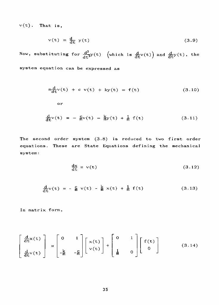
v(t) . That is,

v(t) =^

y(t)dt *vw (3-9)

Now, substituting for ^1y(-t) (which is ^v(t)) and jf^yO) >the

system equation can be expressed as

"dtv(t)+ c v(t) + ky(t) = f (t) (3.10)

or

&-<*> = ~ Sv(t) - jjjy(t) + i f (t) (3.11)

The second order system (3.8) is reduced to two first order

equations. These are State Equations defining the mechanical

system :

ar= v^> (3.12)

dt' 00 = -

m v(t)- j x(t) + 1 f(t) (3.13)

In matrix form,

"

&*(*>"

0 1 _ -, 0 1 r

x(t) f(t)+

.

aH*)_

km

c

m

v(t) 1m

0

0(3.14)

35

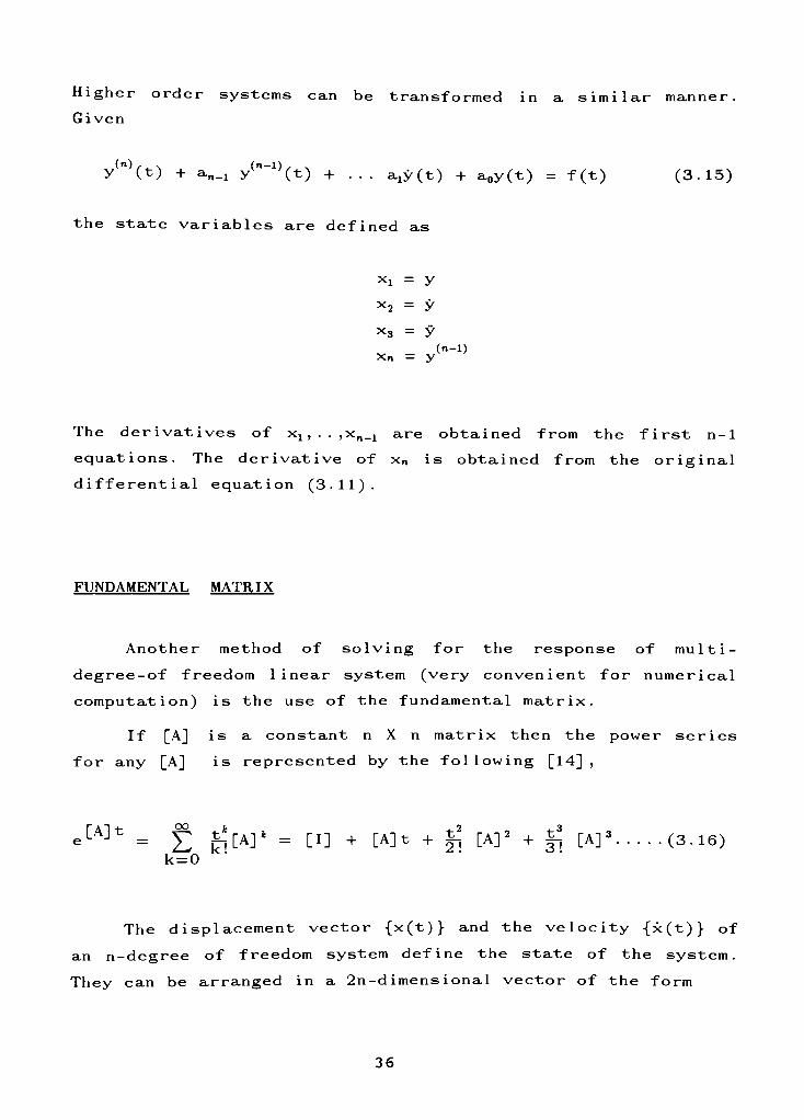
Higher order systems can be transformed in a similar manner.

Given

y(n)(t) + a_t y("_1)(t) + . . . alY(t) + a0y(t) = f(t) (3.15)

the state variables are defined as

Xi = y

x2 = y

x3 = y

(n-l)x = y

The derivatives of x1,..,xn_1 are obtained from the first n-l

equations. The derivative of x is obtained from the original

differential equation (3.11).

FUNDAMENTAL MATRIX

Another method of solving for the response of multi-

degree-of freedom linear system (very convenient for numerical

computation) is the use of the fundamental matrix.

If [A] is a constant n X n matrix then the power series

for any [A] is represented by the following [14] ,

CA]t= = [I] + [A]t +

21

[A]2

+31

[A]3

^3-16)k '

k=ok

The displacement vector {x(t)} and the velocity {x(t)} of

an n-degree of freedom system define the state of the system.

They can be arranged in a 2n-d imensional vector of the form

36

_

f{x(t)}l~

\{*00}J^00} =

T^TTTT (3-17)

Similarly, you can introduce the 2n-dimensional forcing vector

{F(t)} - {im} (3-18)

where {y(t)} is known as the state vector and {F(t)} is the

force vector. The equation of motion of an n-degree of freedom

linear system can be written in the general matrix form,

{y(t)> = [A]{y(t)> + [B]{F(t)} (3.19)

where [A] and [B] are 2n X 2n matrices of coefficients,

depending on the nature of the system.

To obtain a solution of the above equation, first consider

the homogenous equation,

{yO0> = [A]{yO)> (3.20)

This matrix equation is similar in structure to the scaler

first-order differential equation. Letting {y(0)} be the

initial state vector, the solution of the homogeneous equation

above can be verified to be

{y(t)> = e[A]t{y(0)} (3.21)

where e is the series matrix as defined previously in

equation (3.16),

37

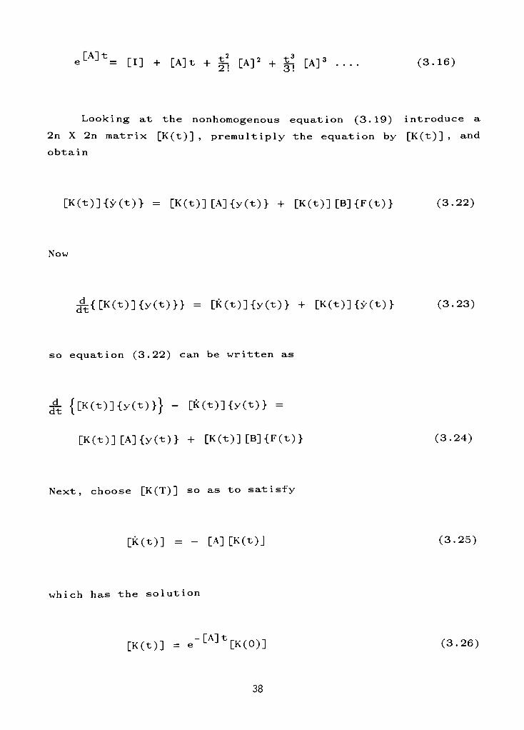
e[A]t= [I] + [A]t +[A]2

+[A]3

.... (3.16)

Looking at the nonhomogenous equation (3.19) introduce a

2n X 2n matrix [K(t)] , premultiply the equation by [K(t)] ,and

obtain

[K(t)]{y(t)> = [K(t)] [A]{y(t)} + [K(t)] [B] {F(t) } (3.22)

Now

^{[K(t)]{y(t)}> = [K(t)]{y(t)> + [K(t)]{y(t)> (3.23)

so equation (3.22) can be written as

^ {[K(t)]{y(t)}}- [K(t)]{y(t)} =

[K(t)] [A]{y(t)} + [K(t)] [B]{F(t)} (3.24)

Next, choose [K(T)] so as to satisfy

[K(t)] = - [A] [K(t)j (3.25)

which has the solution

[K(t)] = e"[A]l:[K(0)] (3.26)

38

For convenience, we choose [K(0)] as the identity matrix, or

[K(0)J = [I] (3.27)

so that equation (3.26) reduces to

[K(t)] = (3.28)

From equations (3.28) and (3.16) we observe that the matrices

[K(t)] and [A] commute (same 2n X 2n order) ,or

[A] [K(t)] = [K(t)] [A] (3.29)

Substituting equation (3.29) into equation (3.25), we can see

the matrix [K(t)] also satisfies

[K(t)J =-[K(t)] [A] (3.30)

so equation (3.24) can be reduced to

A {[K(t)]{y(t)}}= [K(t)] [B]{F(t)}dt

(3.31)

So to complete the solution of equation (3.19), you have to

solve equation (3.31) above. Integrating equation (3.31) yields

[K(t)]{y(t)> = [K(0)]{y(0)> + [K(r)] [B]{F(r)}dr

0

= {y(0)> + | [K(r)] [B]{F(r)}d, (3.32)

39

premultiplying equation (3.32) by [K(t)]_1, yields the solution

of the nonhomogenous equation (3.19) in the form,

{yO)> = [K(t)]"1{y(0)} + | [K(t)]"1[K(r)] [B]{F(r)}d1

0

{y(0)> + | e[A](t-r)[B]{F(r)}dr (3.33)

0

Equation (3.33) contains the same solution as in equation

(3.24) for the homogenous case. Since both the homogenous and

particular solutions are present, this is the complete solution

for equation (3.19).

FORCED SOLUTIONS

The behavior determined by a forcing function is called a

forced response and that, due to initial energy storage, is the

natural response. The time between the starting and the ending

of the natural response is the transient response. After the

natural response has become negligibly small, conditions are

said to be in steady state.

The differential equation of motion for a second order

linear system (mass-damper-spring) with arbitrary forcing f(t)

is

mx (t) + cx(t) + kx(t) = f(t) (3.34)

where the excitation force, f(t), is chosen to be harmonic. The

simplest form is

f(t) = Acos(ut) (3.35)

40

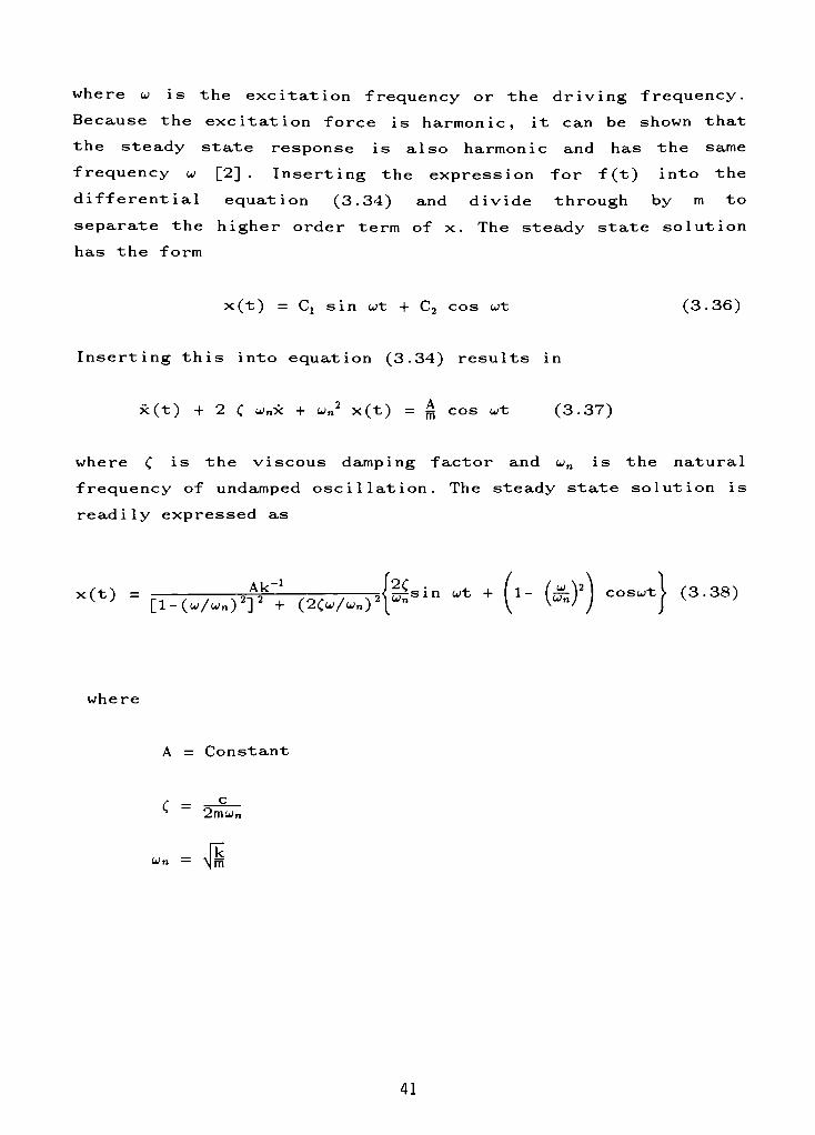
where w is the excitation frequency or the driving frequency.

Because the excitation force is harmonic, it can be shown that

the steady state response is also harmonic and has the same

frequency u [2]. Inserting the expression for f(t) into the

differential equation (3.34) and divide through by m to

separate the higher order term of x. The steady state solution

has the form

x(t) = Cj sin wt + C2 cos wt (3.36)

Inserting this into equation (3.34) results in

x(t) t 2 ( wx +w2

x(t) = ^ cos wt (3.37)

where is the viscous damping factor and un is the natural

frequency of undamped oscillation. The steady state solution is

readily expressed as

:(t) =-A^

J^sin ut +K J [l-(u-/W)2]2

+ (2(U/W)2i

(l-()2j cosu,tj

(3.38)

where

A = Constant

c~

C

2mwn

U)n =>[S

41

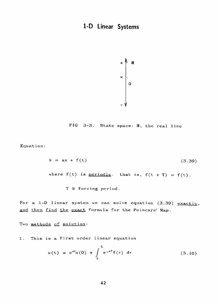
1-D Linear Systems

+ f R

0

FIG 3-3. State space: R, the real lint

Equat ion :

x = ax + f (t) (3.39)

where f(t) is periodic . that is, f(t + T) = f(t).

T = forcing period.

For a 1-D linear system we can solve equation (3.39) exactly .

and then f ind the exact formula for the Poincare'Map.

Two methods of sol ut ion :

1. This is a first order linear equation

t

:(t)= eatx(0) + f e-arf(r) (3.40)

42

2. Use Laplace Transform.

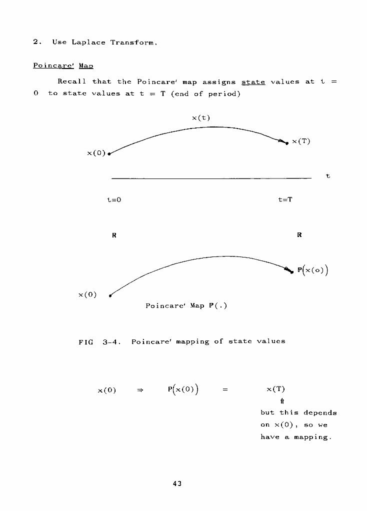
Poincare'Map

Recall that the Poincare'

map assigns state values at t

0 to state values at t = T (end of period)

x(0)

x(t)

:(T)

t=0 t=T

R R

x(0)

Poincare'

Map P(.)

(x(o))

FIG 3-4.Poincare'

mapping of state values

x(0) P(x(0)) x(T)

ft

but this depends

on x(0) ,so we

have a mapping.

43

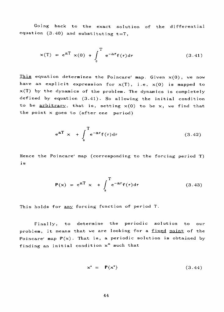
Going back to the exact solution of the differential

equation (3.40) and substituting t=T,

i

x(T) =eaT

x(0) + f e-arf(r)dr (3.41)

This equation determines the Poincare'map. Given x(0) ,

we now

have an explicit expression for x(T) , i.e, x(0) is mapped to

X(T) by the dynamics of the problem. The dynamics is completely

defined by equation (3.41). So allowing the initial condition

"to be arbitrary, that is, setting x(0) to be x, we find that

the point x goes to (after one period)

i

eaT

x + / e~arf(r)dr (3.42)

Hence thePoincare'

map (corresponding to the forcing period T)

i s

i

P(x) =eaT

x + / e-aTf(r)dr (3.43)o

This holds for any forcing function of period T.

Finally, to determine the periodic solution to our

problem, it means that we are looking for a f ixed po int of the

Poincare'

map P(x). That is, a periodic solution is obtained by

finding an initial conditionx*

such that

x*

= P(x*) (3.44)

44

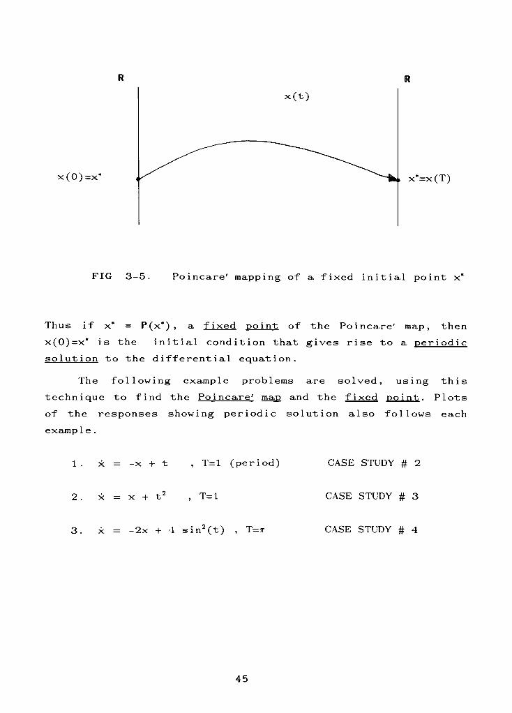
R

x(0)=x*

x'=x(T)

FIG 3-5. Poincare'

mapping of a fixed initial pointx*

Thus ifx*

= P(x*) ,a f ixed point of the

Poincare'

map, then

x(0)=x*

is the initial condition that gives rise to a peri od i c

so 1ut i on to the differential equation.

The following example problems are solved, using this

technique to find the Po incare' map and the f ixed point . Plots

of the responses showing periodic solution also follows each

example .

1. x = -x + t ,T=l (period) CASE STUDY # 2

2. x = x +t2

,T=l CASE STUDY # 3

3. x = -2x + 4 sin2(t) ,T=tt CASE STUDY # 4

45

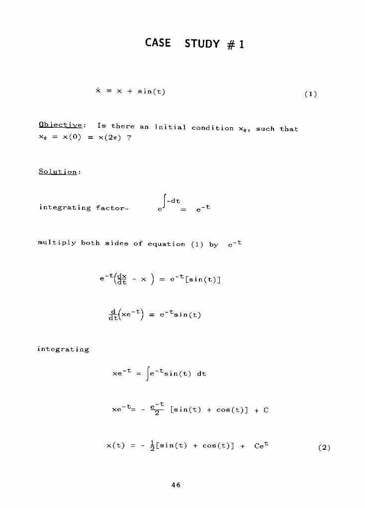
CASE STUDY # 1

= x + sin(t) /-j\

Objective: Is there an initial condition x0 , such that

x0 =x(0) =

x(2?r) ?

Solut ion

-dt

integrating factor- e^

=e-1:

multiply both sides of equation (1) bye-t;

^(dt " X ) =

e^TsinOO]

s(xe_t)=

e"tsin(o

integrat ing

xe-*

e tsin(t) dt

t_e"*

xe = - ^- [sin(t) + cos(t)] + C

xO)= - ^[sin(t) + cos(t)] +

Ce^

46

(2)

Define constairt c in t^s rf .^.^ ^.^ ^xQO) =

x0, so from (2) ,

Xn = J[0 + 1] + c

x0 = - i + C

C =x0 +

1

*00 = -

j[sin(t) + cos(t)] +xoe*

+ letie (3)

this is the solution forarbitrary x0 .

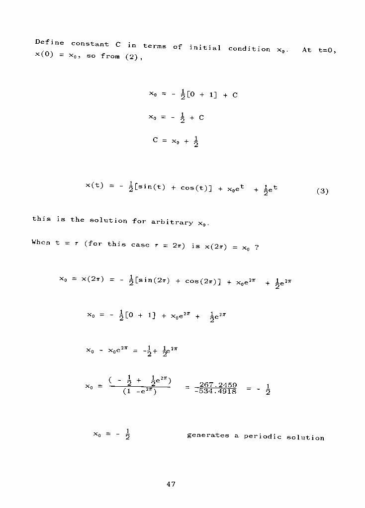
When t = r (for this case r = 2tt) is x(2t) =x0 ?

-

x(2t) = - i[sin(27r) + cos(2i)] +x0e2,r

+Ie27r

Xn = ^[0 + 1] +x0e2T

+le2*

x0 x0e _

~2+9

C - I + Ie27rNlxn =

22e

>>

_ 267.2459^o 1

(1-e2*) -534.4918 2

x0 =1

2 generates a periodic solution

47

LJ

CO

O

CL_

CO

LJ

Oi i

E-h

O

CO

o

a

o

LJ

c._>

CO

+

X

I

X

CO

o

- tx

CD

LO

CD

-P

to

cm

SZ"0 OS'O SS'O OO'O SrTO- 0S'0-9Z"0-

mx

48

CASE STUDY #2

Ql2^-:X = -X + t (1)

Qbiective: Find the limit of any solution ?

Solut ion :

[dtintegrating factor- eJ

=e*

multiply both sides of equation (1) bye(

Ute Hx + x =

el

t)

d_/_0 _e,

tdt("')

integrat ing

xe1

=e'

t dt

:'=(t-l)e'

+ C

x(t)= (t-1) +

Ce"'

(2)

49

Define constant C in terms of initial condition x0 . At t=0 ,

x(0) =x0, so from (2) ,

*o = (0 -

1) + C

xo = - 1 + C

C =x0 + 1

x(t) = t - 1 +Xoe-'

+e"'

*<(x) = t - 1 +xe-<

+e"*

this is the solution for arbitrary x.

The Poincare'

map is given by

1x1 = *T(x) = T - 1 +xe"T

+e-T

Solving for initial condition x0 from (3) ,

x0 = t - 1 +x0e_<

-)-

e-<

x0-

x0e-'

= t - 1 +e-'

x(l -

e-') = t - 1 +e-t

=( * ~ * + e-)

(1-e"')

50

(3)

(4)

(5)

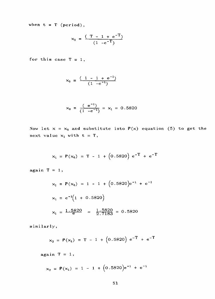
when t = T (period) ,

( T - 1 + e~T)x0 =

(1-e"T)

for this case T = 1,

x- < 1 ~ 1 + e-1)

X "

(1-e-)

_( e-1)

(1 -e~0

xn =t^

^- =xj

= 0.58201 -e l)

Now let x = x0 and substitute into P(x) equation (5) to get the

next value xx with t = T,

-T -T

e1

+ el

xj = P(x0) = T - 1 + (0.5820)

again T = 1,

Xl= P(x0) = 1 - 1 +

(0.5820)e_1+e_1

Xl = e_1(l + 0.5820)

v_

1 .5820 _1 .5820 _ 0 =o20

xi=

e-

2.7183" -5^u

s imi lar ly ,

x2= P(xJ = T - 1 + (o.582o)

e~T

+

again T = 1 ,

x2= P(xi) = 1 - 1 +

(o.582o)e"1+e"1

51

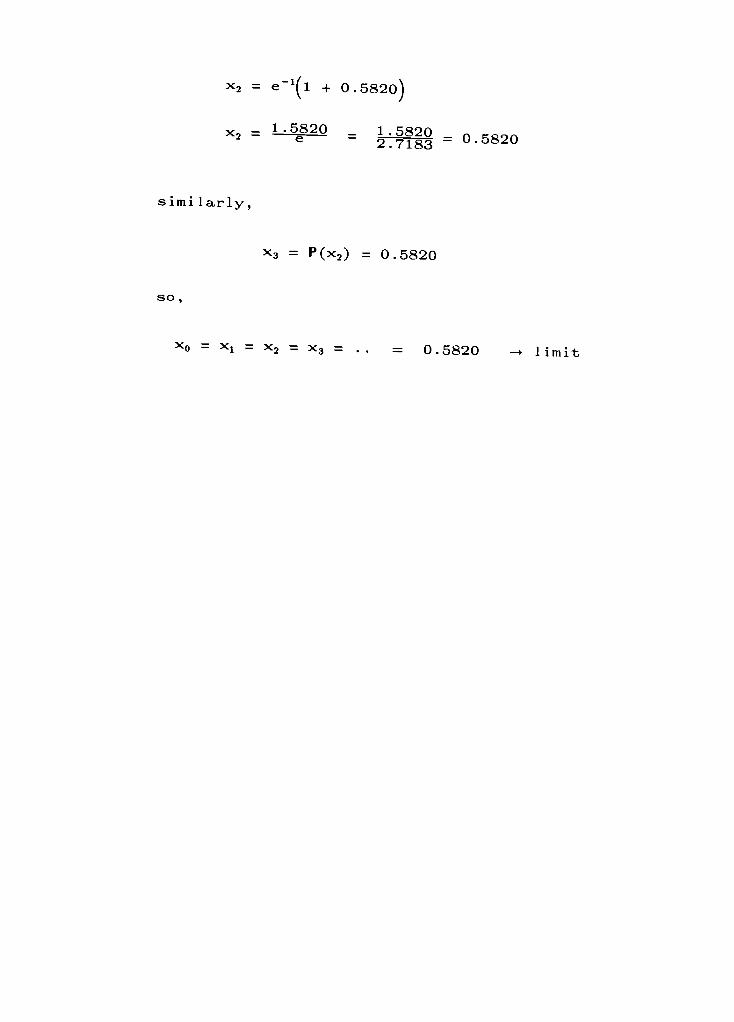
x2 = e x(l +0.5820)

x_ 1 . 5820 l 5820X2 e

=

2 . 7183= -5820

simi larly ,

x3 = P(x2) = 0.5820

so ,

x0 -

xx =x2 =

x3 =. . = 0.5820 - limit

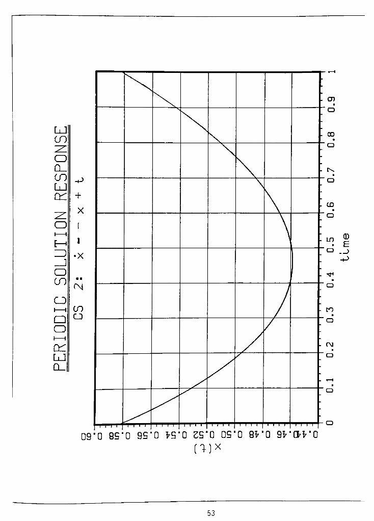
LJ

CO~^

o

CL_

CO-p

LJ

C +

ZX

o [

1 1

E~ 1

ZDX

_J

o

CO

CJ1 1 CO

QO

oi i

a:

LJ

a_

09'0 89'0 99*0 *9"0 29*0 09'0 8*'Q 9VOVQ

53

CASE STUDY #3

a^^:X = x +

t2

(1)

Obiective: Find the limit of any solution ?

Solut ion

[-dtintegrating factor- eJ

=e-1

multiply both sides of equation (1) bye_t

((af + x ) =e- t'

&(*-') =e_t *'

integrat ing

xe"'

=e_t

t2dt

From CRC handbook,

x(t)= - t2- 2t - 2 +

Ce'

(2)

54

Define constant C in terms of initial condition x0 . At t=0 ,

x(0) = x0, so from (2),

x0 = - 2 + C

C = x0 + 2

x(t) = - t2- 2t - 2 + [x0 +2]e*

(3)

this is the solution for arbitrary x0 .

When t = r (period) ,

P(x) = - r2- 2r - 2 + [x0 + 2]er

(4)

Solving for initial condition x0 (3),

x0=t2

- 2t - 2 -I-

x0e'

+2e'

x0-

x0e'

= -

t2- 2t - 2 +

2e*

x0(l -

e')= -

t2- 2t - 2 +

2e*

(- t2- 2t - 2 + 2e')

x0=

(1 -e<)

when t = r,

(- r2

- 2r - 2 + 2er)X

"

(1 -er)

55

for this case r = 1,

(- 1 - 2 - 2 + 2(2.7182818)X

(1 - 2.7182818)

( - 5 + 5.43656)(-

1.7182818)

x0 = - 0.25406 = Xl = - 0.25406

Now substitute x0 into P(x) equation (4) to get the next value

x2 with t = r,

x2 = P(xx) = - r2- 2r - 2 + [x0 + 2]er

again r = 1 ,

x2= P(xx) = -1-2-2+

[- 0.25406 + 2] 2 . 7182818

x2= - 0.2505

simi larly ,

x3= P(x2) = - 0.2505

so

xn = Xl= x2

= x3= ..

= - 0.2505 - limit

56

LJ

CO

O

Q_

CO

LJ

Oi i

E-

O

CO

O

Q

O

LJ

-P

+

x

i

X

CO

CO

o

092 "0-9ZZ"0- 00'0- 9S'0- 09"0- 9Z"08{tf'0-

57

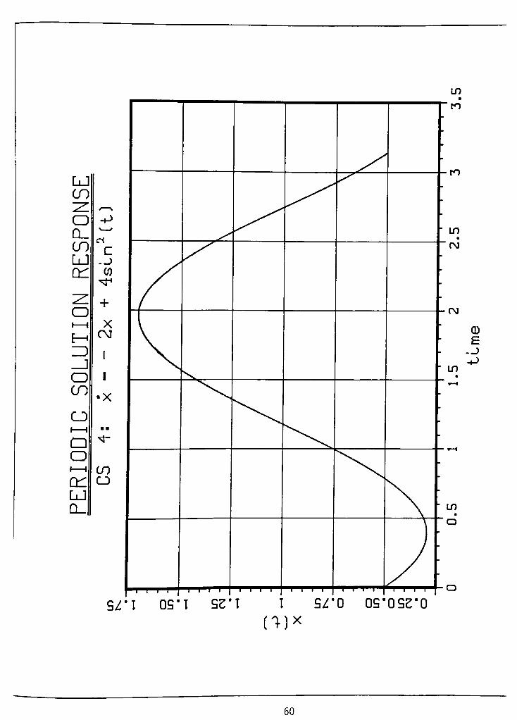
CASE STUDY # 4

x = -2x + 4sin2(t) (1)

Objective : Find the periodic solution, i.e. the initial

condition (IC), such that x0= x(0) = x(n-) .

Solut ion :

From Maple [9] the solution to (1) is

x(t) = | - ^2" +x(0)e_rt

-

cos2

t - sinttcost (2)

which is the solution for arbitrary x0 . At the initial

condition, x(0)=

x0 ,solve (2) for x0

x(0)=

x0= ^

- + x0e - cos t - sinttcost

For t = T (period) = n

3e"2(,r)

-2< if n / N /A

x0= %

- ^=

12+ x0e - cos (ir) - s l n (7r) cos (tt)

f \ -7. (it)-20) 3 e i e \ t \ r \

x0- x0e =

^"

;2" OS ^ ~

sin(7r),cos('r)

Co(l _

e-25r

) = | " ^T"

(-1)2- (0).(-l)

4(* -

e'2*)_

i

(l -

e""

)"

2Xn =

58

Using the Poincare'map , Xl =

x0 , x2 = P(xJsubstitute the value for Xl into equation (2)

3 Q~2

-,

x2 _

2~ "2" + ^2^e ~

cos t - sinttcost

After another period, t = T = n

3e_2,r

1 -

x2 =

2" "2" + ^2-^e ~

cos2(*0-

sin(7r)cos(7r)

i -

Sr +c)e-8*

-

(-1)2- (o).(-i)

v- 3 e , /l\_-2ir .

X2 -

2" ^2~ + ^e ~ 1

x- I

x2 -

2

Since

xo xx x2 . . .

75

we can conclude that we have found a Period ic solution which

is also a fixed po int

x0= xx = x2 . . .

= i fixed point

59

LJ

CO

:z:

o

0_

CO

LJ

Oi i

O

CO

CJ

Q

O

a:

LJ

a

c

CO

X

CM

I

I

X

CO

o

9Z'I09'

I 92*1 0S"QSZ'0

(l)x

60

Higher Dimensional Systems

Now looking at the equation for a 2-D linear system (mass

spring) ,

rax + kx = f(t) (3.45)

where f(t) is periodic, f(t + T) = f(t)

T= forcing period

For a 2-D system, the approach for solving is similar to that

for a 1-D system. The difference is that now there is a system

of equations instead of one equation. There are two methods

st

for solving systems of linear 1 order equations:

[1] Fundamental solutions

The 2 order linear system for a mass spring setup is

mx + kx = sin(t) (3.46)

Convert the equation to two linear 1 order state equations by

using,

y = x (3.47)

Equation (3.45) then becomes

my + kx = sin(t) (3.48)

61

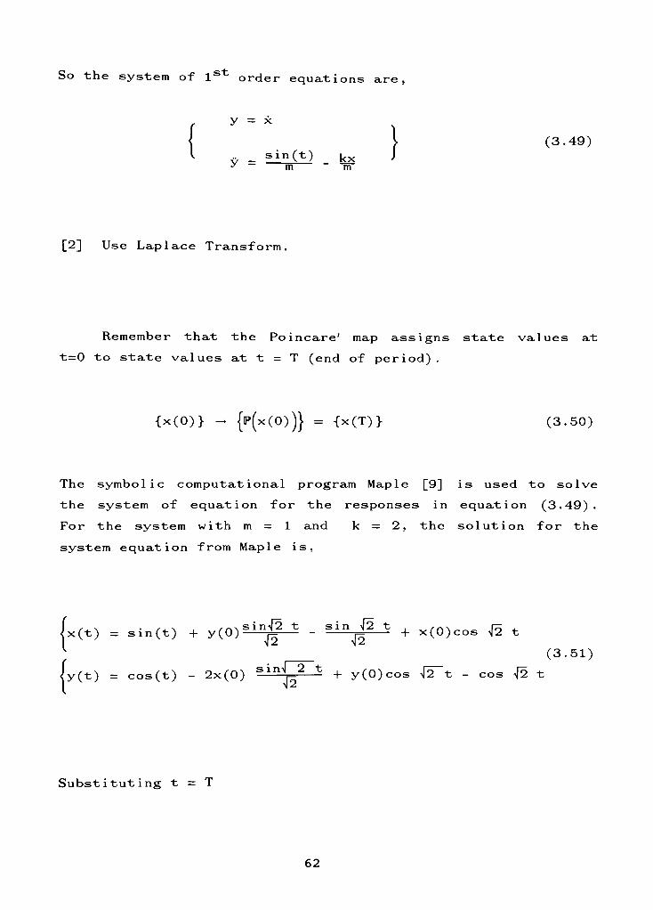
So the system of1st

order equations are ,

\ (3.49)

_ sin(t) kx Jy

~

m m

[2] Use Laplace Transfo rm .

Remember that the Poincare'

map assigns state values at

t=0 to state values at t = T (end of period) .

{x(0)} - {P(x(0))} = {x(T)} (3.50)

The symbolic computational program Maple [9] is used to solve

the system of equation for the responses in equation (3.49).

For the system with m = 1 and k = 2, the solution for the

system equation from Maple is,

|x(t) = sin(t) + y(0)sinjj?

*-

"in& *+ x(0)cos ^2 t

[(3.51)

|y(t) = cos(t)- 2x(0) Sin]

U2 *+ y(0)cos

J2~

t - cos ^2 t

Substituting t = T

62

(T) =cos(T)

-

2x(0) sinj|T

+ y(0)cos J2 T - cos ^2 T

(3.52)

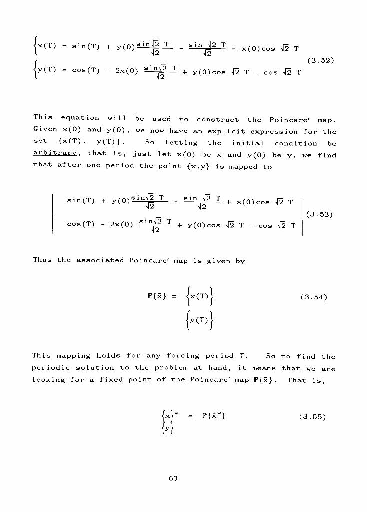
This equation will be used to construct the Poincare'map.

Given x(0) and y(0) , we now have an explicit expression for the

set {x(T) , y(T)}. So letting the initial condition be

arbitrary, that is, just let x(0) be x and y(0) be y, we find

that after one period the point {x,y} is mapped to

sin(T) + y(0)simf2 T

42

in 42 T

42+ x(0)cos 42 T

cos(T)-

2x(0) sin^T

+ y(0)cos 42 T - cos 42

(3.53)

Thus the associatedPoincare'

map is given by

P{x} (3.54)

This mapping holds for any forcing period T. So to find the

periodic solution to the problem at hand, it means that we are

looking for a fixed point of thePoincare'

map P{x} . That is,

(3.55)

63

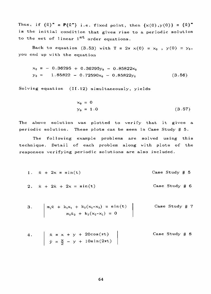
Thus, if{x}*

= P{x*> i.e. fixed point, then {x(0),y(0)> =

{x}*

is the initial condition that gives rise to a periodic solution

to the set of linearls^

order equations.

Back to equation (3.53) with T = 2w x(0) = x0 , y(0)= y0 ,

you end up with the equation

x0 = - 0.36295 + 0.36295y0 -

0.85822x0

y0 = 1.85822 - 0 . 72590x0 - 0.85822y0 (3.56)

Solving equation (11.12) simultaneously, yields

x0 = 0

Yo = 1-0 (3.57)

The above solution was plotted to verify that it gives a

periodic solution. These plots can be seen in Case Study # 5.

The following example problems are solved using this

technique. Detail of each problem along with plots of the

responses verifying periodic solutions are also included.

1 . x + 2x = sin(t)

x + 2x + 2x = sin(t)

Case Study # 5

Case Study # 6

itiiX + kjXj + k2(xx-x2) = sin(t)

m2x2 + k2(x2-x1) = 0

Case Study # 7

4. x = x + y + 20cos(7rt)

y=x

-

y + 10sin(27rt)

Case Study # 8

64

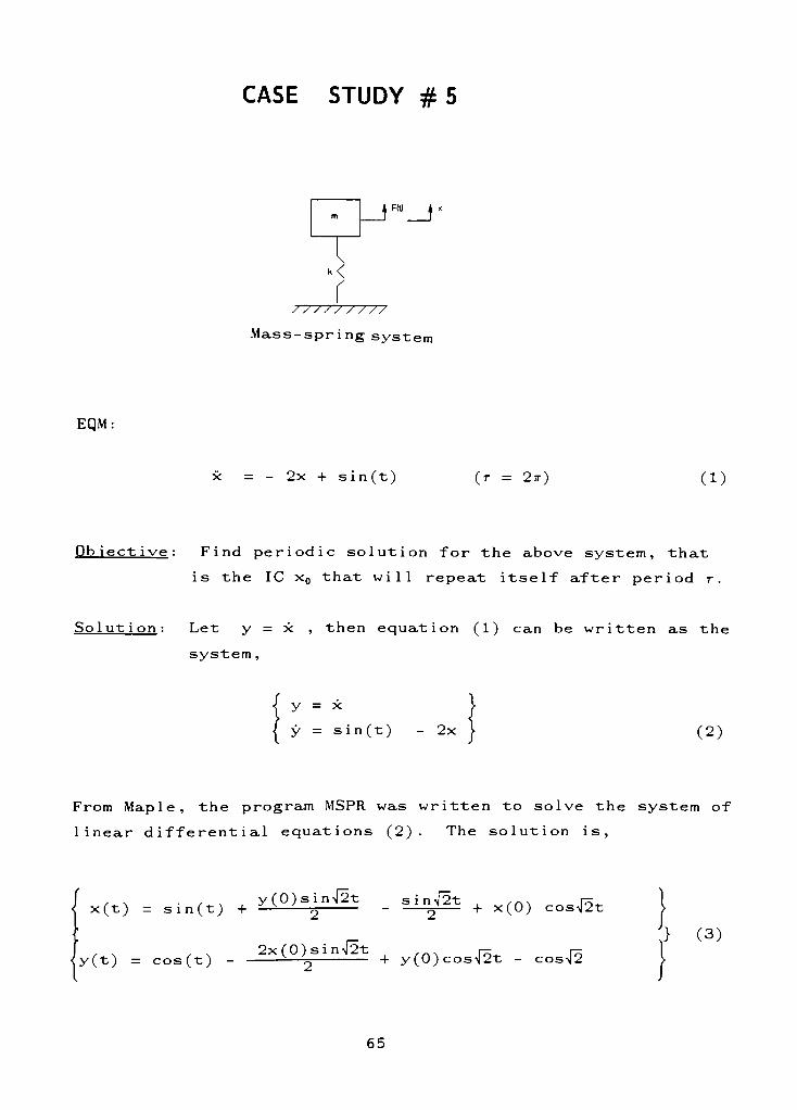
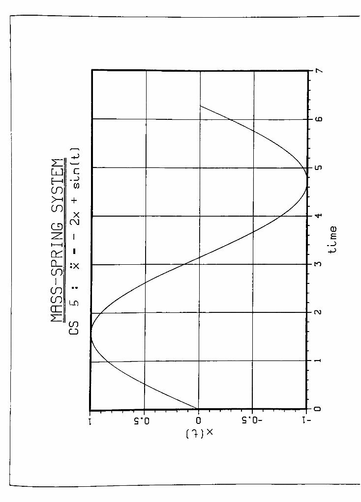
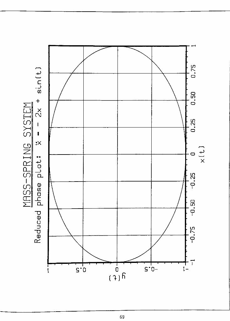
CASE STUDY # 5

F(1>

1

Mass-spring system

EqM:

x = - 2x + sin(t) (r = 2*) (1)

Ob iect ive : Find periodic solution for the above system, that

is the IC x0 that will repeat itself after period r.

Solut i on : Let y = x , then equation (1) can be written as the

system,

y = x

y = sin(t)- 2x (2)

From Maple, the program MSPR was written to solve the system of

linear differential equations (2). The solution is,

x(t) = sin(t) +y()S2n^

- ^^ + x(0) cos42t 1

<y(t) = cos(t)-

2x(0)sin42t+ y(Q)cos^ _

cos^

} (3)

65

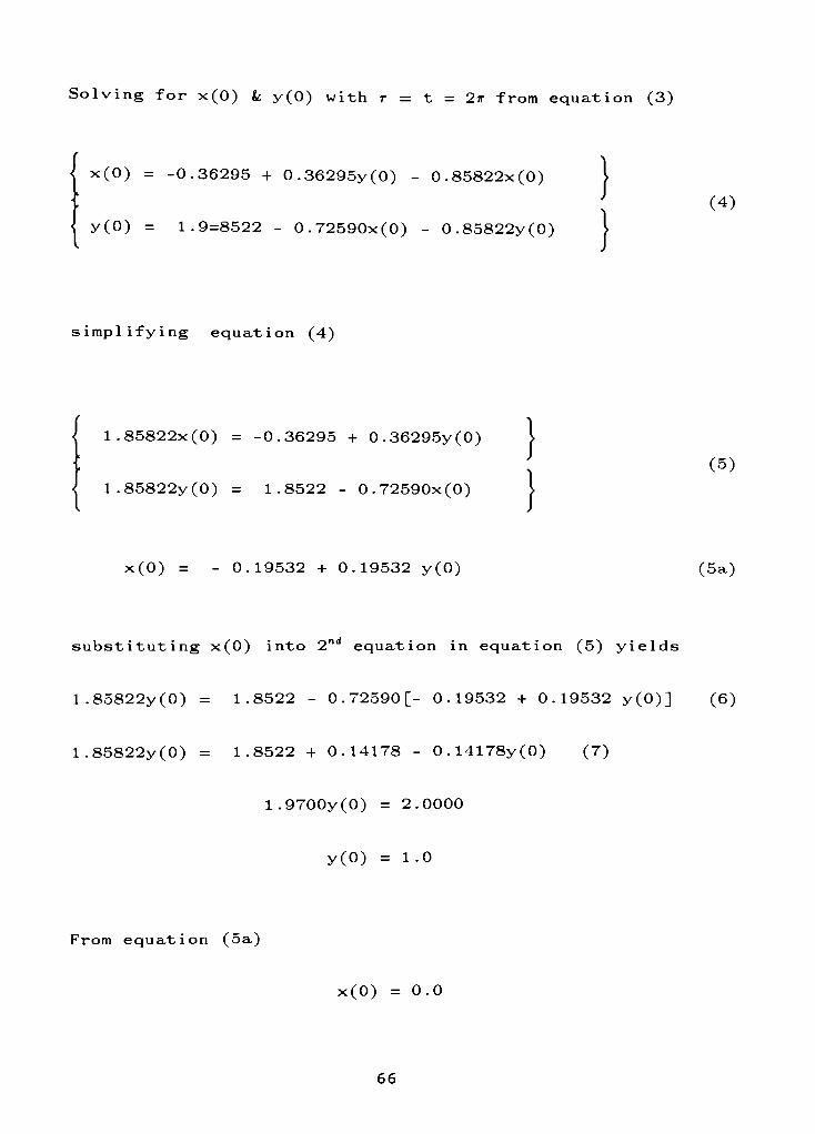
Solving for x(0) k y(0) with r = t = 2n from equation (3)

x(0) =-0.36295 + 0.36295y(0) - 0.85822x(0)

y(0) = 1.9=8522 -

0.72590x(0) - 0.85822y(0)

))

(4)

simplifying equation (4)

1.85822x(0) = -0.36295 + 0.36295y(0)

1.85822y(0) = 1.8522 -

0.72590x(0)

)

)(5)

x(0) = - 0.19532 + 0.19532 y(0) (5a)

substituting x(0) into2"

equation in equation (5) yields

1.85822y(0) = 1.8522 - 0.72590[- 0.19532 + 0.19532 y(0)] (6)

1.85822y(0) = 1.8522 + 0.14178 - 0.14178y(0) (7)

1 .9700y(0) = 2.0000

y(0)= 1.0

From equation (5a)

x(0)= 0.0

66

The initial condition giving rise to a periodic solution is

x(0)= 0.0

y(0) = 1.0

The following plots verify that the above values found give

rise to a periodic solution.

67

-P

LJ c

E-

COCO

>H +

COX

CDCM

21 1

i i

C1

CL. :x

CO

1

COa

CO1-0

eny~

CO

o

CD

-P

LJ

CO

CO

CD

Q_

CO

I

CO

CO

en

c

CO

X

CM

rX

-P

o_)

Q_

CD

CO

O

Q_

"O

0

CJ

"D

CD

cr:

9'0 09*0-

o

LT)

IT)

CN

-P

X

IT)OO

oI

o

in

oi

ID

I-

mR

69

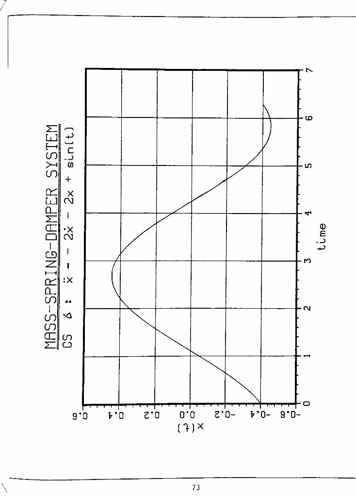
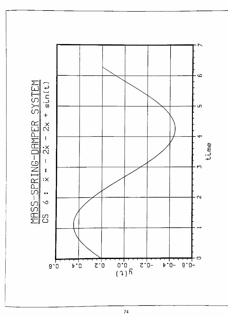
CASE STUDY # 6

Fffl X X. X

k < O =

/////////

Mass-spring-damper system

EQM:

x = -2x- 2x + sin(t) (r = 2w) (D

Ob iect i ve : Find periodic solution for the above system, that

is the initial condition x0 that will repeat itself

after period r.

Sol ut i on : Let y = x,then equation (1) can be written as the

system,

y = x

y = sin(t)- 2x - 2x (2)

From Maple, the program MSPRD was written to solve the system

of linear differential equations (2). The solution is,

x(t)= y(0)e"'sin(t) +

ge 'sin(t) +

x(0)e~*

+ 2e-'cos(-,-)

+ x(0)e"'cos(t) + isin(t) - ^cos(t) I(3)

70

| YOO = -

2x(0)e-<sin(t) - 3e-sin(t;) _ Ie-cos(t;)

-

y(0)e-sin(t) + y(0)e-'cos(t) + cos(t) + Isin(t) | (4)

Now solve for x(0) with t = r = 2* from equation (3)

| x(0)=x(r) =

y(0)e-Tsin(r) +1e-rsin(r) +

x(0)e-r

+ e-rcos(r) + x(0)e-rcos(r) + Jsin(r) - cos(r) ]

simplifying [dropping sin(r = 2?r) = 0],

2 -r

x(0) = ge rcos(r) + x(0) e_rcos (r) - 2cos(r)

x(0) = g[1.8674(10-3)] + x(0) [1.8674(10-3)] - \

x(0) [1 -

1.8674(10-3)] = |[1.8674(10-3)] -

|

0.998x(0) = - 0.39925

x(0)= -0.39997

Similarly, solve equation (5) for y(0) with t = r = 27r,

71

y(0) =y(r) = - 2x (0) e-rs i n (r) - 2e-rsin(r) - le-rcos(r)

-

y(0)e-rsin(r) + y (0) e-rcos(r) + Icos(r) + 2sin(r)

Simplifying [dropping sin(r = 2tt) = 0],

y(0) = - ie-Tcos(r) + y (0)e-rcos (r) + lcos(r)

y(0) = - i[1.8674(10~3)] + y (0) [1 . 8674 (10~3)] + 1

y(0) [1-

1.8674(10-3)] = - i [1 .8674 (10-3)] + 1

y(0) [.998] = 0.19963

y(0) = 0.20

The initial condition giving rise to a periodic solution is

x(0)= - 0.4

y(0)= 0.2

Plots of the above values verified the periodic solution

72

mx

73

LJE-

CO

CO

en

LJ

Q_

CC

Q

I

CD

on

Cl.

CO

I

CO

CO

en

CD

-P

i i i

0"b Z'O- v'O- 9"0-

(1)R

74

LJE-h

CO

CO

cl:

lj

Cl.

z:

en

o

i

CD

Cl.

CO

I

CO

CO

cn

-p

c._>

CO

+

CM

X

oo

I

I

:X

-P

o

CD

CO

O

_c

D_

"TJ

CD

OD

"D

CD

. -P

X

O'O Z'O- v'O- 9"0-

75

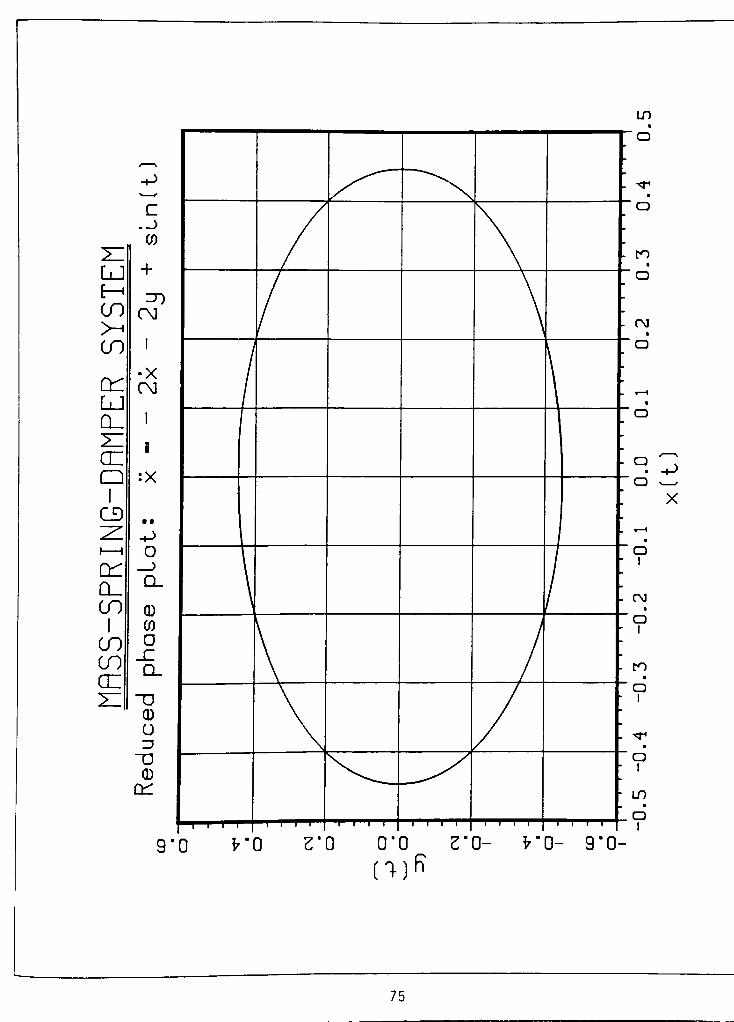
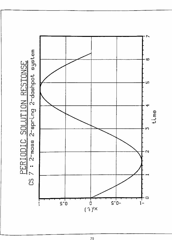
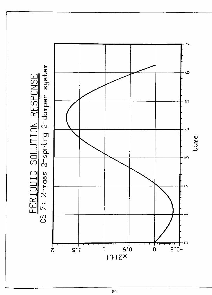
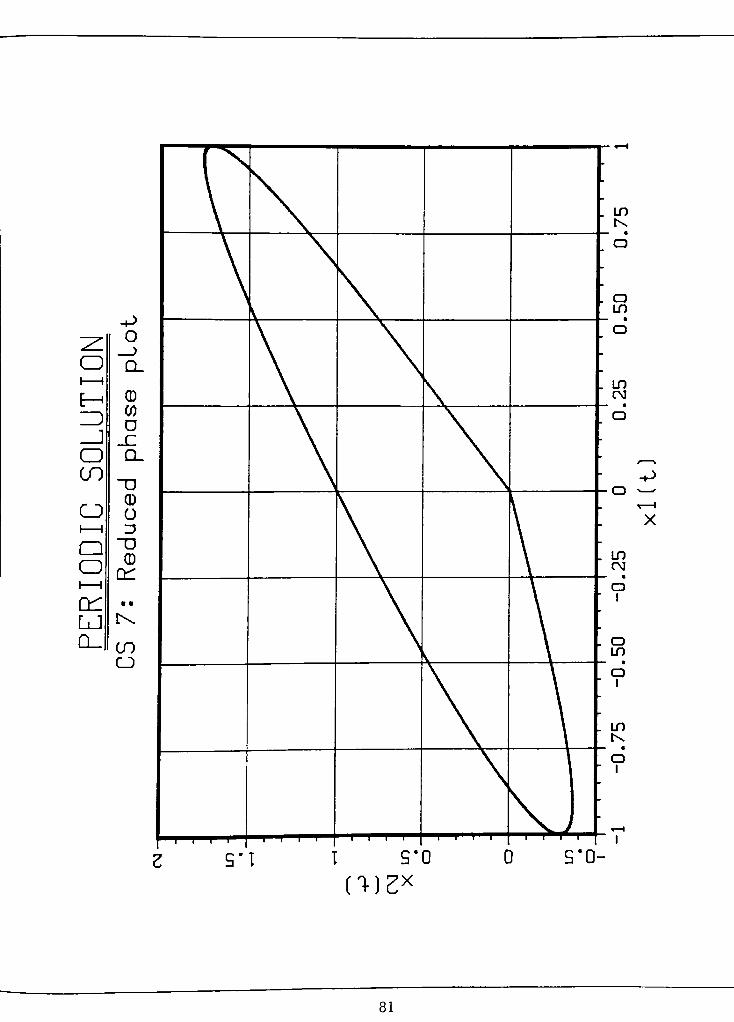
CASE STUDY #7

F(t)

Ob iect ive : Find periodic solution for the above system, that

is the Initial Conditions that will repeat itself

after period r.

So 1 ut ion : From the differential equation of motion (EQM) ,

then arrange the system equations in simultaneous

first order form, by letting xx=

vx k x2=

v2 , state

equat ions .

EQM:

kjXi -

CjXi + k2(x2 -

xL) + c2(x2-

xx)=m^j

F(t) - k2(x2-

xx)-

c2(x2-

xx)= m2x2

(1)

(2)

Rearrangi ng ,

mixi + (cL + c2)x!-

c2x2 + (kt + k2)x!- k2x2 - 0

m^Xo ^2^1 " ^2^2 k2Xj + k2x2 = F(t)

(la)

(2a)

76

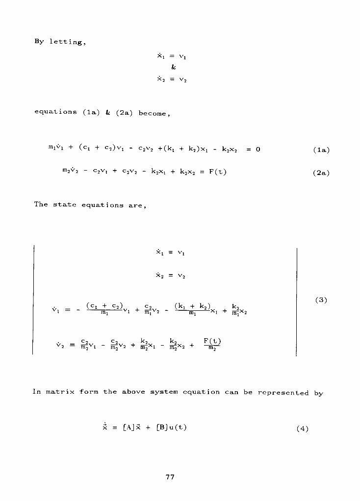
By letting,

Xi =vx

k

x2 =v2

equations (la) k (2a) become,

"xVi + (cx + c2)Vl-

c2v2 +(kj-I-

k2)Xl - k2x2 = 0

m2V2

-

C2V! + c2V2-

k2X! + k2X2 = F(t)

(la)

(2a)

The state equations are,

xi =Vi

x2 =v2

(ci + c2>vi +

mfv2

(ki + k2),k

m, xi + ffqx2

_<-2

v2 fri;vi~

m;v2 + frwxik2 k,

^ F(t)rnix2 +

m,

(3)

In matrix form the above system equation can be represented by

x = [A]x + [B]u(t) (4)

77

For the case with no damping.

cx =c2 = 0

Using the following values

equation (3) become

k2 = ki = 1

nij =m2 = 1

F(t) =sin(t)

x, = v,

x, = v,

vi = -

2xj + x2

=xx

-

x24-

sin(t)

(5)

The program, Twomass, (Maple) was used to solve the system of

linear first order equations in (5). The initial condition

giving rise to a periodic solution for the system is,

Xl(0)= 0.0 ; x2(0)

= 0.0 ; vx(0) = -1.0 ; v2(0) = -1.0

The Assystant phase plotting software, was used to verify the

periodic solution. Example plots are on the following pages.

78

0

-P

LJ

CO

CO

CO"^

CD -p

E-h

CO

u

r

LJ CO

rr D

"TJ

zz.1

CM

o1 1 CD

E-> C

fZD

_J Q_

O CO

CO1

CM

o CO

1 1 CO

a

1oi i OO

en

LJ

Q_ IX

CO

o

79

0

LJ II -*->

CO

=T)CO

~Z_ CO

o

CO

L

0

0.

LlJ

ctr. D

TJ

~z_1

CM

o1 1 CD

E-h C

f

_J CL

O CO

CO1

CM

o CO

1 1 CO

CD

O 1i i OO

on

LJ

Cl.

a

tX

CO

CJ

CD

LO

0

-P

-P

to

CM

S"T I 9'0 9'0-

80

-P

81

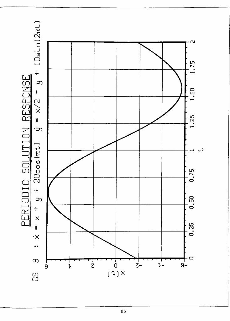
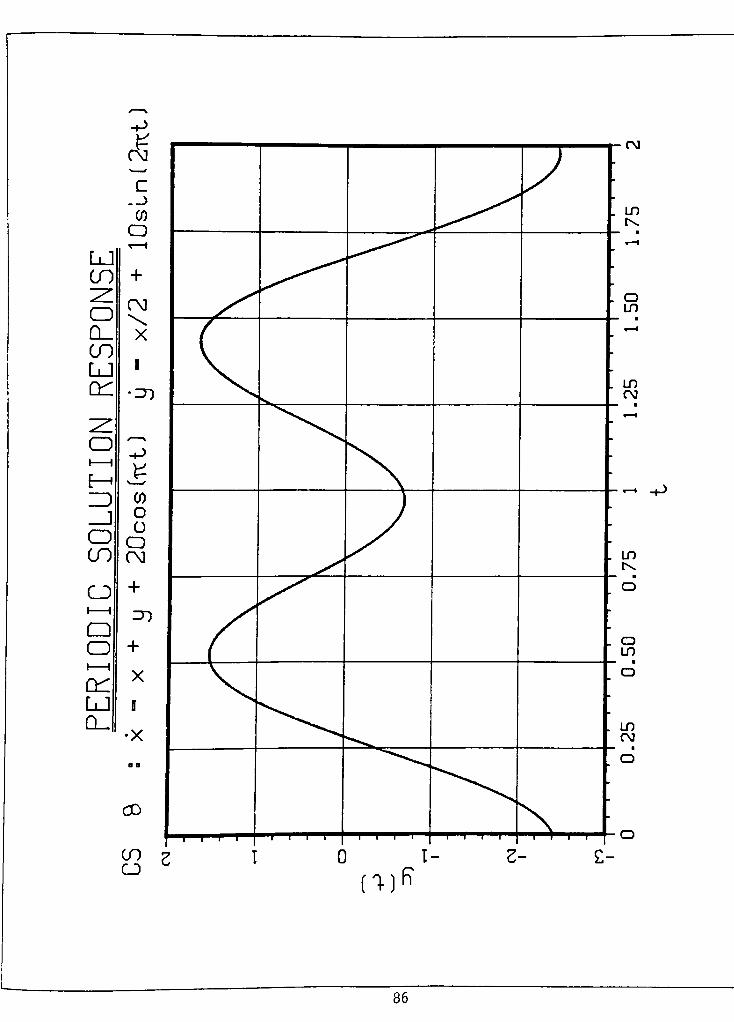
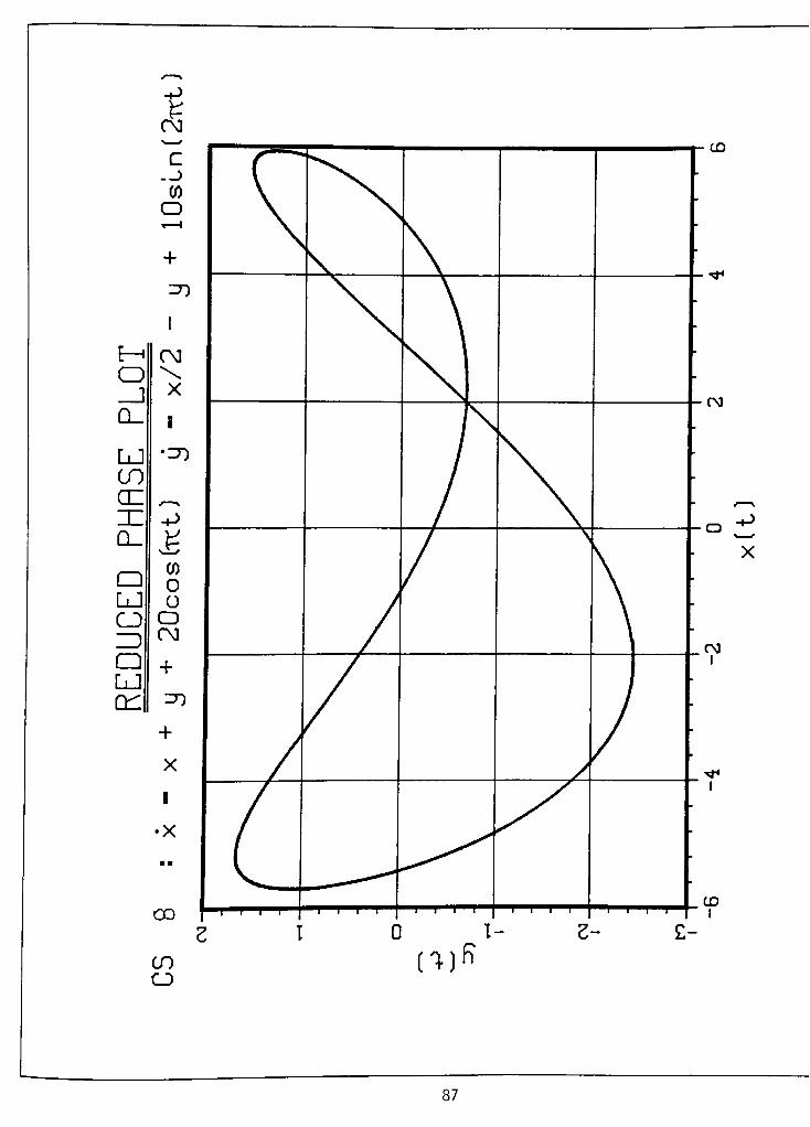
CASE STUDY # 8

Given: The linear differential equation set

x = x + y + 20cos(wt)

y = |-

y + 10 sin(27rt)

(1)

Objective: Find periodic solution for the above system

equations, that is the Initial Conditions

that will repeat itself after the period r.

Solution : From equation (1) above, Maple was used to solve foi

the solution x(t) and y(t)

xftN

_ [Acosh(At) + sinh(At)]x0 + sinh(At)y0

A

30?T +16?r4

+ 9

[320*2

+ 120cosh(At) +l(807r3

+480*2

+ 180 -f 1207r)sinh(At) + (- 40tt2-

60) sin (2;rt)]

, ,_

(A2- l)sinh(At)x0 + [Acosh(At) -

sinh(At)]{X,) - T

Yo+

60

-^---l-[(120 +320;r2

+ 240*) cosh (At) +7T + ,3Zir + 18

(-160,3-

240,)s.nh(At)] _40,cos(2,t)3 +

8tt'+

82

20sin(27rt)3 +

8tt2

20cos(rt)2tt2

+ 3

where3

N2

After substitution for the value of A (1.224745), the above

expressions for x(t) k y(t) simplifies to

x(t) = 3.4063sinh(l,224745t) + 1 . 7591cosh (1 . 224745t)

1.7591cos(irt) + x0cosh(l

.224745t)- 0 . 2440s in (2*t)

+ 5.5263sin(7rt) + 0 . 8165x0sinh (1 . 224745t)

+ 0.8165sinh(l.224745t)y0

y(t) = 2.4128cosh(l.224547t)

- 1 . 2519sinh (1 . 224745t)

+ 0.4082x0sinh(l.224745t) + y0cosh (1 . 224745t)

- 0.8165sinh(l.224745t)y0

- 0.8795cos(7rt)

+ 0.2440sin(2irt) - 1 . 5333cos (?rt)

For this problem, with two separate forcing functions, the

period is T = 2. Upon substitution for t = T in the above

expression, and with x(2)= x0 and y(2)

= y0 ,the requirement

for a periodic solution reduces to

x0= 28.0834 + 10.5276x0 + 4 . 6933y0

y0= 4.4684 + 2.3466x0 + 1.1411y0

solving simultaneously, the initial condition giving rise to a

periodic solution is

83

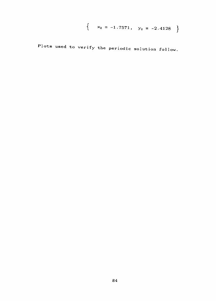
{ x0 =

-1.7571, y0 =-2.4128 }

Plots used to verify the periodic solution follow.

84

-P

OO

c-_>

CO

0r 1

+

LJ

CO =D

2!1

O1

Q_ OO

CO \

LJX

en 1

^ U)

O1 1

E--P

ID

_J

CO

0O

CO 0

0

OCM

1 1+

O

O =T)

1 1

CLl+

LJ X

CL.1

X

CO

CO

CJ

CM

LT>

tx

oIT)

LOCM

IT)

tx

o

m

IT)CM

Z- *- 9-

-P

(1)x

85

-p

CM

C._>

CO

oT 1

LJ

CO +

OCM

CL_ X

CO

LJa

en '=T)

zz.

o-P

1 1

E-h

ZD CO

_J

O

o

o

CO CM

CD+

i i^o

Q

O +

i i

enX

LJ I

Q-lX

OD

00 ?CJ

C

-P

86

-p

Yoo

c._)

CO

oT 1

+

=T)

E-h

1

oo

O \

_J

X

CL I

LJ -^r>

CO

cn /^^

m -p

CL

CDCO

0

LJ o

Cl o

DDCM

CD +

LJ

en ="

+

X

i

X

-CD

CO

CO

o

-P

X

87

IV NONLINEAR SYSTEMS

The study of nonlinear systems is more complicated than

the study of linear systems, which can be attributed to the

fact that the superposition principle (the ability to add

linearly the responses of a system to various excitations) is

not valid for nonlinear systems. This leads to an entirely

different approach for handling nonlinear systems. Numerical

methods are usually needed for solving nonlinear system

equations. It should also be pointed out that the theory of

nonlinear differential equations is not as complete as that for

linear differential equations. In addition, it relies heavily

on approximations based upon linear theory. There are

circumstances where it is possible to use methods of linear

theory in the study of nonlinear systems by examining the

motion in the neighborhood of known motions, a process referred

to as linearization. This is the basis of Lyapunov's First

Method [2] .

There are two basic approaches to solving nonlinear

systems, the qualitative and the quantitative method. The

qualitative approach is concerned with the general stability

characteristics of the system in the area of a known solution,

rather than with the explicit time history of the motion. On

the other hand, the quantitative approach is also concerned

with the time histories. Such solutions can be obtained by

pertubation methods or by numerical integration.

This paper will investigate an area of the qualitative

approach by focusing in the neighborhood of a known solution of

the system, the periodic solution (if it exists). To begin

with we need to introduce the Infinitesimal Generator operator

which can be used in the analysis.

88

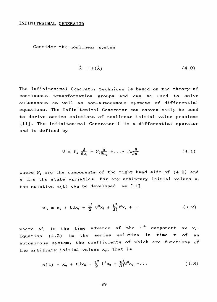
INFINTTE.STMAI, GENERATOR

Consider the nonlinear syster

= F(x) (4.0)

The Infinitesimal Generator technique is based on the theory of

continuous transformation groups and can be used to solve

autonomous as well as non-autonomous systems of differential

equations. The Infinitesimal Generator can conveniently be used

to derive series solutions of nonlinear initial value problems

[11] . The Infinitesimal Generator U is a differential operator

and is defined by

U = F* A +

F>A+--'+ ^n <4-1}

where F; are the components of the right hand side of (4.0) and

x, are the state variables. For any arbitrary initial values x^

the solution x(t) can be developed as [11]

x*,. = x; + tUx,. + ^ U2x< + ^U3x,- +. . . (4.2)

wherex*

is the time advance of the i component ox x, .

Equation (4.2) is the series solution in time t of an

autonomous system, the coefficients of which are functions of

the arbitrary initial values x0 ,that is

x(t)= x0 + tUx0 + ^ U2x0 + fJ3x0 +. . . (4.3)

89

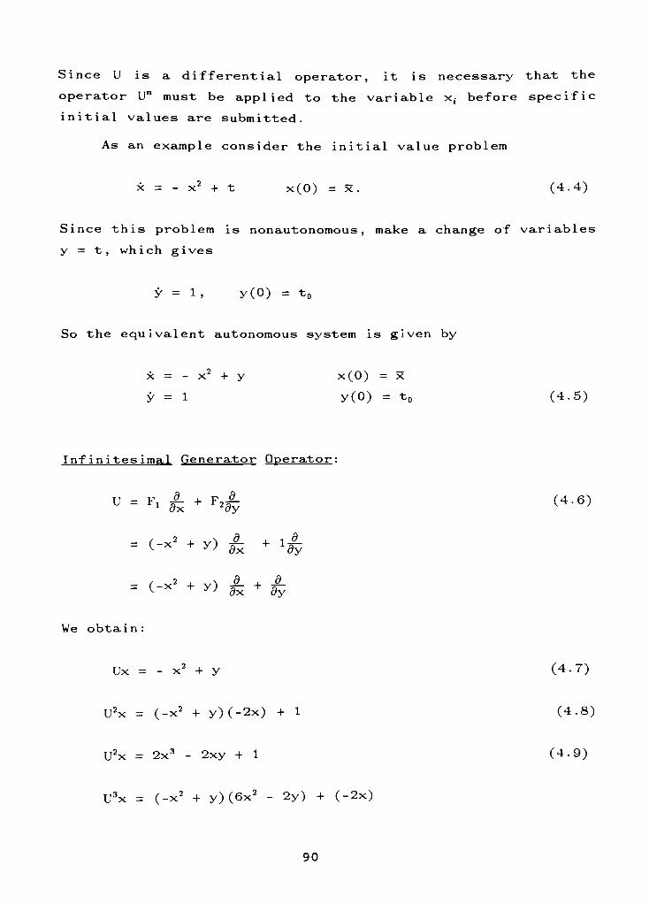
Since U is a differential operator, it is necessary that the

operatorU"

must be applied to the variable x, beforespecific

initial values are submitted.

As an example consider the initial value problem

x = -

x2

+ t x(0) = x. (4.4)

Since this problem is nonautonomous, make a change of variables

y = t, which gives

y = 1, y(0) = t0

So the equivalent autonomous system is given by

x = -

x2

+ y x(0)=x

y = 1 y(0)= t0 (4.5)

Inf initesimal Generator Operator :

U = F1#- + F2- (4.6)1dx 'dy

c2

+ y) &- ^

=(-*'

+ y)cfe

+dy

=<-*'

+ y) fe +'dy

2 , .^ d L d_

We obtain

Ux = -

x2

+ y (4.7)

U2x =

(-x2

+ y)(-2x) + 1 (4.8)

U2x =

2x3- 2xy + 1 (4.9)

U3x =(-x2

+y)(6x2

- 2y) + (-2x)

90

= -

6x4

+ 8x2y -

2y2- 2x (4.10)

U4x =(-x2

+y)(-24x3

+ 16xy - 2) +(8x2

- 4y) (4.11)

And

Uy = 1 (4.12)

U*y = 0 for all k > 2 (4.13)

Maple software can be used to solve for the series expansion.

The program code for doing the partial derivatives and

calculating the expansion for a 2-D system of equation is the

program VECFLD2D in Appendix A. All you have to do is define

the two variables xx and x2 and the two functions Fx and F2

(first order differential equations) .

Final ly :

'ith h = time advance

:(h) =xh

= x +(-x2

+ y)h +(2x3

- 2xy + 1 ) j^ +

(-6x4

+ 8x2y -

2y2- 2x)^ + [U4x] ^ + ... (4.14)

y"

= y + 1(h) = y + h (4.15)

Now substitute initial conditions:

x"

= x +(-x2

+ t0)h +(2x3

- 2xt0 + 1)^, +h

+(-6x4

+ 8x2t0 -

2t02-

2x)j^, + [U4x]^, + (4.16)

91

where x = x, y = t0

yh

= t0 + h (4.17)

x, y are values of the state variables after a time-advance

of"h"

.

The series solution can now be expressed as a mapping

G(x,t0,h) = x + (-x2+ t0)h +(2x3

- 2xt0 + 1)^-I-

. . . .

+(-6x4

+ 8x2t0 -

2t02-

2x)^ + [U4x]j^ + (4.18)

with derivative

2

DG(x,t0,y) = 1 + (-2x)h +(6x2

-

2t0)J-j +

+(-24x3

+ 16xt0 -

2)^ + Dr[U4x]^ + (4.19)

The fixed point was found to be

x0 = 0.7867627.

See Appendix A for the program Test. for that was used to solve

for the fixed point of thePoincare' Map. The following figure

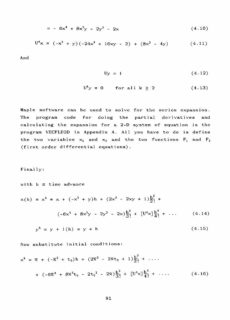
FIG 4-1, shows the relation between the input function and the

convergence of the initial guess to the fixed point.

92

INPUT

INITIAL

GUESS

0.7867...

FIXED POINT

Ut)

^4

x(t)

FIG 4-1. System input and output side by side

while seeking periodic solution

Example: Solve using Infinitesimal Generator,

x = + tx x(0) = x0

The initial value was found to be

x0= 0.5428

See example Case Study # 9 ,at the end of the 1-D Nonlineai

Systems section, for detailanalysis of this example problem.

93

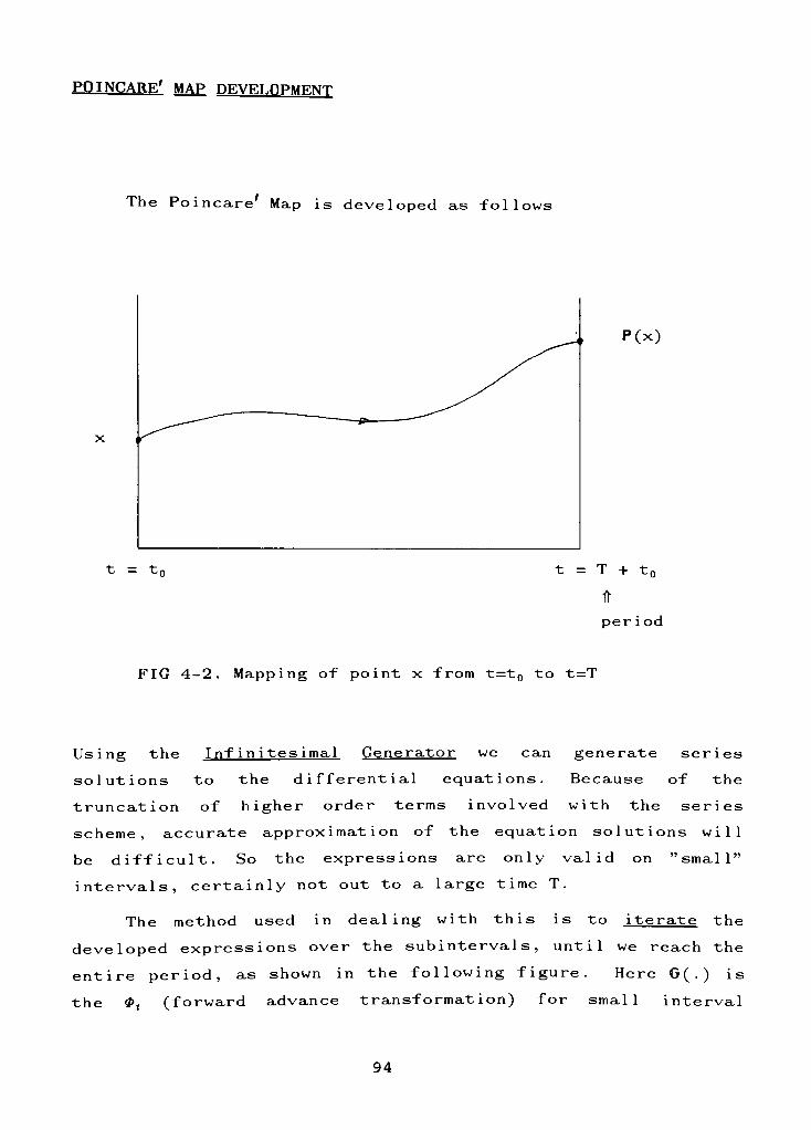
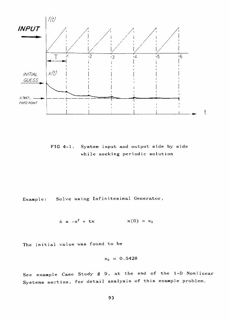
POINCARF/ MAP DEVELOPMENT

The Poincare'

Map is developed as follows

P(x)

t = tr T + t0

it

period

FIG 4-2. Mapping of point x from t=t0 to t=T

Using the Inf in itesimal Generator we can generate series

solutions to the differential equations. Because of the

truncation of higher order terms involved with the series

scheme, accurate approximation of the equation solutions will

be difficult. So the expressions are only valid on"small"

intervals, certainly not out to a large time T.

The method used in dealing with this is to iterate the

developed expressions over the sub i nterval s , until we reach the

entire period, as shown in the following figure. Here G(.) is

the $t (forward advance transformation) for small interval

94

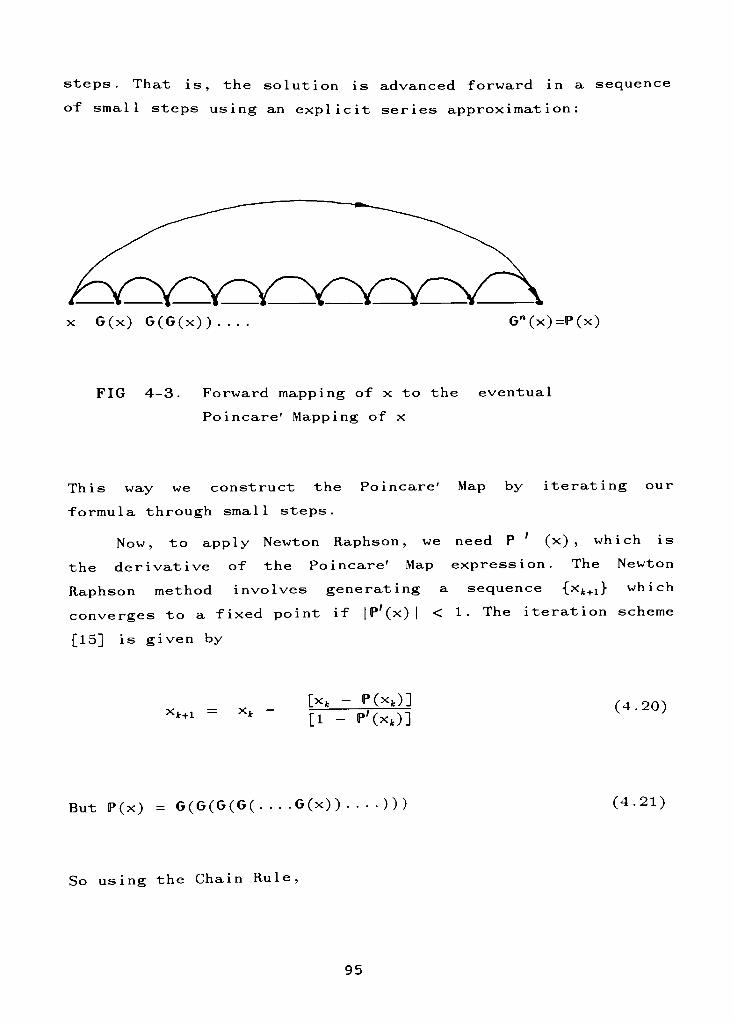
steps. That is, the solution is advanced forward in a sequence

of small steps using an explicit series approximation:

x G(x) G(G(x)) . . . . Gn(x)=P(x)

FIG 4-3. Forward mapping of x to the eventual

Poincare'

Mapping of x

This way we construct thePoincare'

Map by iterating our

formula through small steps.

Now, to apply Newton Raphson,

we need P'

(x) ,which is

the derivative of thePoincare'

Map expression. The Newton

Raphson method involves generating a sequence {xt+1} which

converges to a fixed point if |P'(x)| < 1. The iteration scheme

[15] is given by

"fc+i= xt

-

[xt - P(xt)]

[1 - P'(xt)](4.20)

But P(x) = G(G(G(G( G(x)) ))) (4.21)

So using the Chain Rule

95

P'(x) = G'(G(G (x)..)) * [G(G(G...(x)...)]

'

(N-l) iterate (N-l) iterate

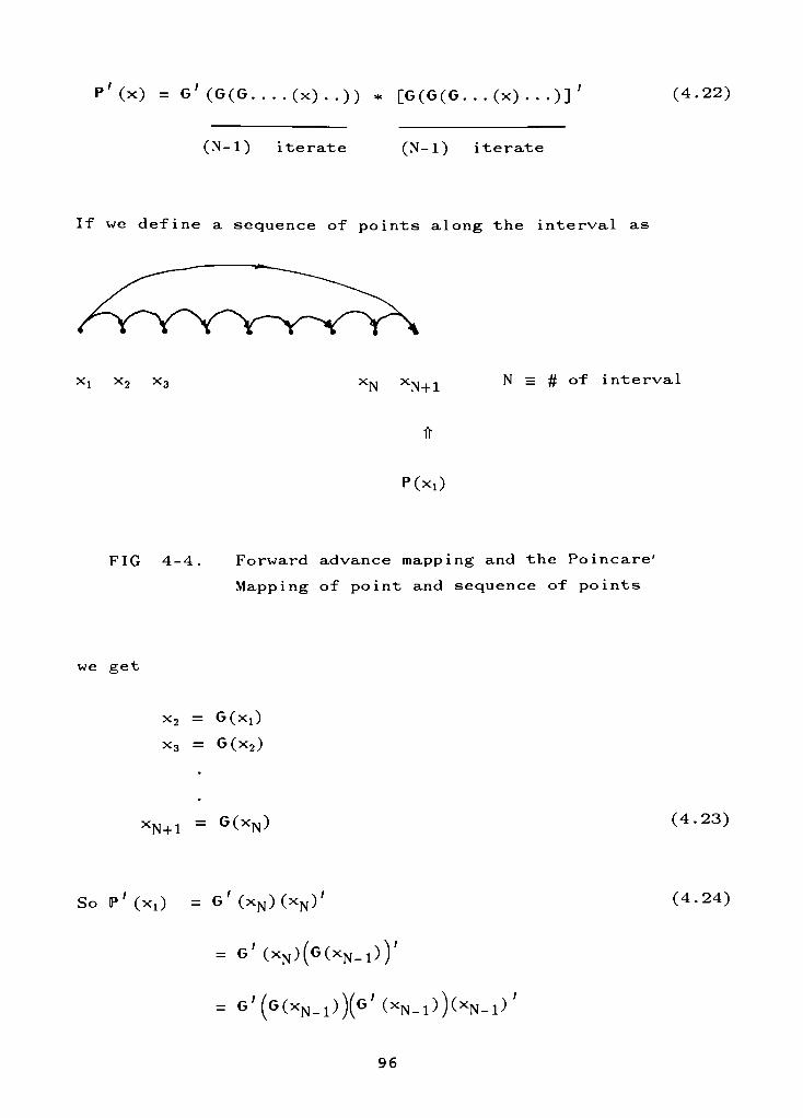
If we define a sequence of points along the interval as

(4.22)

xi x2 x3 XN XN+1

ir

N = # of interval

POO

FIG 4-4. Forward advance mapping and thePoincare'

Mapping of point and sequence of points

we get

x, =

GOO

G(x2)

XN+1= G(XN> (4.23)

SoP'

(xx) =

G' (xN)(xN)'

=

G'(xN)(G(xN_1))'

=

(4.24)

96

=G' (G(xN-l))[G(G(xN_2))]'(xN_1)'

=

G'(xN)G,(G(xn_2))g'(xn_2)(xN_x)'

=G' (xN)G' (x^^G'

(xn_2) . . (xx)

Alternatively ,

P(x) = Gn(x) (n iterations)

= G(G-1(x)) (4.25)

So P'(x) = G'(G"-0(G"-1(x)) (chain rule) (4.26)

Proceeding inductively,

P'(x) =

G'(G"-OG'(G"-2(x))...G'(G(x))G'(x) (4.27)

So again,

P'

(x) =

G' (xN)G' (xN_1)G'

(xN_2) . .

(x2)G'

(Xl) (4.28)

I

I

X = X,

This is the method we will use to seek periodic solutions

for nonlinear systems. Given x = F(x,t), set up G(x), the

forward advance map for "small xintervals"

, and then calculate

G (x) . Apply Newton Raphson to get the best x value for that

interval and then increment that x-value forward by the

incremental amount. Keep repeating this process until x has

been incremented (by the interval amount) over the entire

period. The x-value at the end of the period is the fixed point

for that system.

97

Outl ine of Methodology

Given : A dynamical system, from which we deduce a forward

advance approximation G(x) and then estimate

the Poincare'

map as P(x) =Gn

(x) .

Objective : To find x0 such that P(x0) = x0 , that is establish a

fixed point of P(x) .

Now, once we have P(x) and P'

(x) ,use Newton-Raphson (N-R) to

iteratively find a fixed point:

xl+1 =xt

-

[X* ~ ^X^(4.29)

[1 - P'(xt)]k ;

Now, how does N-R work? Choose an initial guess Xguess, and

use equation (4.29) until

Ixjh-j-

xj < e

where e is some specified accuracy.

Now given Xj. , a N-R iterate, how to actually compute xt+1 ?

Step 1 . Set Xguess= x,.

Step 2. Determine P(xt) and P'(xt). That is compute

P(xt) = G"(xt) = G(G(... G(xt)...) (4.30)

where n = T in which T is the forcing period.

h

98

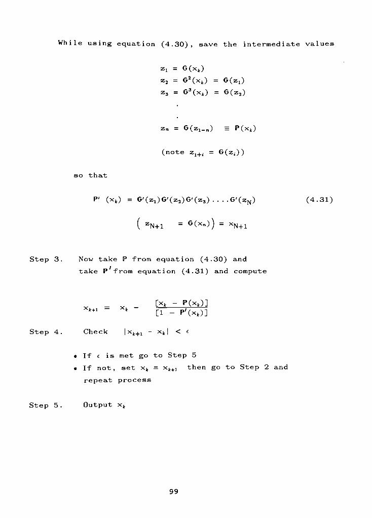
While using equation (4.30), save the intermediate values

Zi = G(xt)

z2 = G2(xt) = G(Zl)

z3 = G3(xfc) = G(z2)

z = G(zx_) = P(xfc)

(note z1+l. = G(z0)

so that

P'

(xfc) = G'(Zl)G'(z2)G'(z3) G'(zN) (4.31)

( ZN+1=

G(x">)=

XN+1

Step 3. Now take P from equation (4.30) and

take P from equation (4.31) and compute

c*+i Xj.[xt - P(xt)]

[1 - P'(xt)]

Step 4. Check | xjt+1-

xt | < e

If e is met go to Step 5

If not,set Xj. = xl+1 then go to Step 2 and

repeat process

Step 5. Output Xj.

99

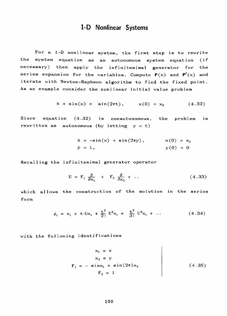
1-D Nonlinear Systems

For a 1-D nonlinear system, the first step is to rewrite

the system equation as an autonomous system equation (if

necessary) then apply the infinitesimal generator for the

series expansion for the variables. Compute P(x) and P'(x) and

iterate with Newton-Raphson algorithm to find the fixed point.

As an example consider the nonlinear initial value problem

x + sin(x) =sin(2wt) , x(0) =

x0 (4.32)

Since equation (4.32) is nonautonomous, the problem is

rewritten as autonomous (by letting y = t)

x =-sin(x) + sin(27ry),

y = l,

x(0) = x0

y(0) = o

Recalling the infinitesimal generator operator

u = F* A + F2 A + (4.33)

which allows the construction of the solution in the series

form

2 3

0,- = x, + t-Ux, + ^U2x,- + J, U3x; + (4.34)

with the following identifications

x, = x

x2= y

Fi = -

sinx! + sin(27r)x2

F2 = 1

(4.35)

100

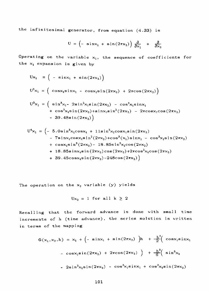
the infinitesimal generator, from equation (4.33) is

U = (-sinx, +

sin(2,x2))jL + JL

Operating on the variable Xj , the sequence of coefficients for

the Xj expansion is given by

Uxx = ( -

sinxj +sin(2irx2)]

U Xj = f cosxisinxj-

cosx^ in (2ttx2) + 2?rcos(2?rx2) J

U Xj = f sin3xr 2sin2Xjsin (27rx2) -

cos2x1sinx1

+ cos xxsin (25rx2)+sinx1sin2(27TX2) - 2icosx!Cos (27rx2)

-

39.48sin(2:rx2))

U4Xj = (- 5 . 0sin3x1cosx1 + 1 lsin2x1cosx1sin(2ix2)

- 7sinx1cosx1sin2(2fx2)+cos3(x1)sinx1 -

cos3x1sin(2?rx2)

+ cosx1sin3(27rx2)- 18 . 85s in2x1cos (2irx2)

+ 18 . 85sinxxsin (2ttx2) cos (2?rx2) +2?rcos2x1cos (2ttx2)

+ 39 . 45COSXJS i n (2ttx2) -248cos (2ttx2) J

The operation on the x2 variable (y) yields

Ux2 = 1 for all k > 2

Recalling that the forward advance is done with small time

increments of h (time advance), the series solution is written

in terms of the mapping

G(x1,x2,h) = xx + (-sinx; + sin(2?rx2) jh + -^-

( cosx^inx!

- cosx!sin(25rx2)-I- 2ttcos (27rx2) J + -j&-( sin3xt

- 2sin2X!sin(27rx2)-

cos2x1sinx1 + cos2x1s in (2ttx2)

101

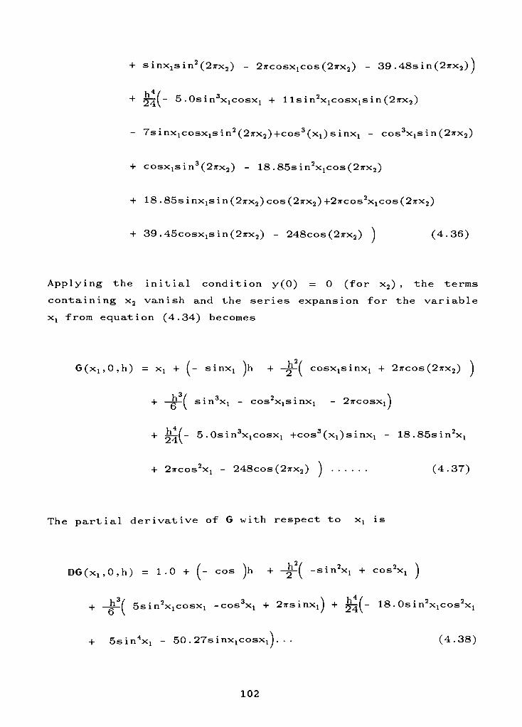
+ sinx1sin2(2n-x2)- 2icosx1cos (2ttx2) - 39 .48sin (2irx2) J

h4

(+ 24v-5.0sin Xjcosxj + llsin2x1cosx1sin(2wx2)

-

7sinx1cosx1sin2(2tx2)+cos3(x1)sinx1 - cos3Xjsin (2n-x2)

+ cosx1sin3(27rx2)- 18 . 85sin2x1cos(27rx2)

+ 18.85sinx1sin(2irx2) cos (2Tx2)+2;rcos2x1cos(2-x2)

+ 39.45cosx1sin(2irx2) - 248cos (2;rx2) ) (4.36)

Applying the initial condition y(0) = 0 (for x2) ,the terms

containing x2 vanish and the series expansion for the variable

x: from equation (4.34) becomes

G(xj,0,h) = Xj + ( -

sinxj jh +-( cosxjsinxj + 2ircos (27rx2) j

+ *? i sin3xx-

cos2x1sinx1-

27TCOSX!)

+ tj-tI- 5 . Osin3x1cosx1 +cos3(x1)sinx1-

18.85sin2X!

+ 2ttcos2x1- 248cos(2ttx2) ) (4.37)

The partial derivative of G with respect to xx is

DG(xl50,h) = 1.0 + (- cos )h +-^ -sin2Xl + cos2Xl )

+ -4r-( 5sin2x1cosx1 -cos3Xj + 27rsinx1J + r^- 18 . 0s in2x1cos2x1

+ 5sin4X!- 50.27sinx1cosx1). . . (4.38)

102

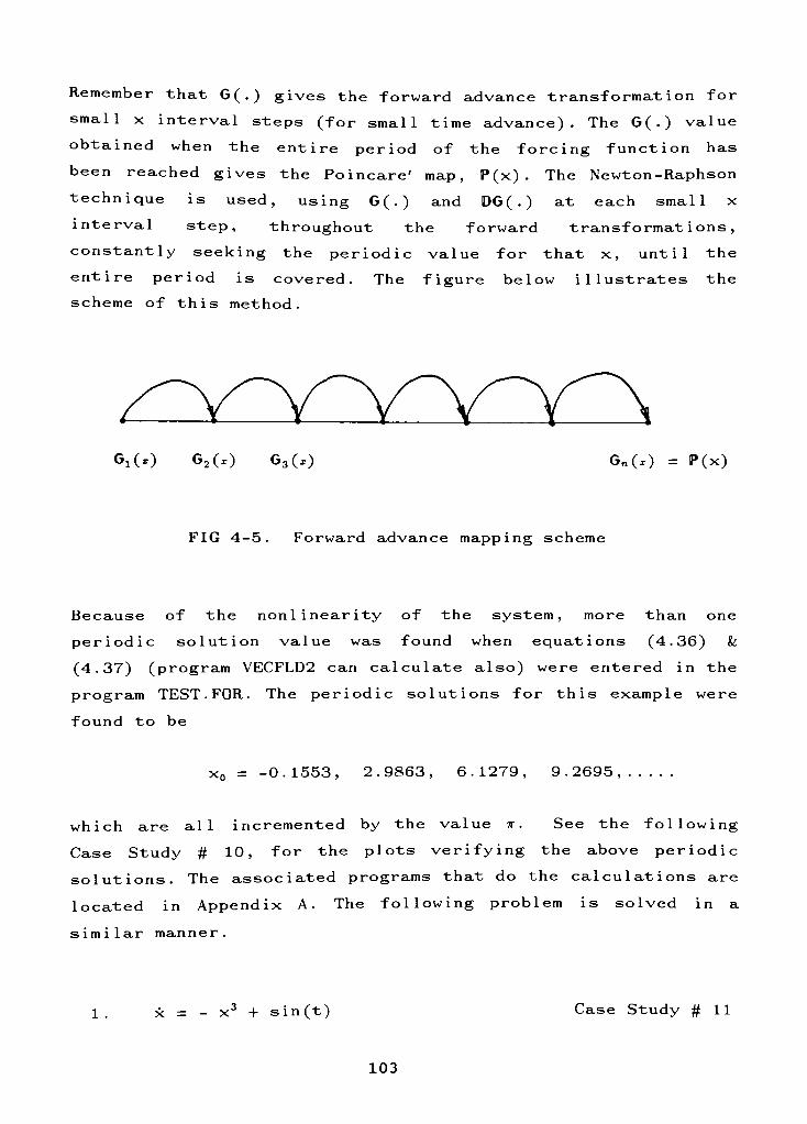
Remember that G(.) gives the forward advance transformation for

small x interval steps (for small time advance). The G(.) value

obtained when the entire period of the forcing function has

been reached gives the Poincare'map, P(x) . The Newton-Raphson

technique is used, using G(.) and DG(.) at each small x

interval step, throughout the forward transformations,

constantly seeking the periodic value for that x, until the

entire period is covered. The figure below illustrates the

scheme of this method.

GiO) G2(*) G3(.) G0) = P(x)

FIG 4-5. Forward advance mapping scheme

Because of the nonlinearity of the system, more than one

periodic solution value was found when equations (4.36) k

(4.37) (program VECFLD2 can calculate also) were entered in the

program TEST . FOR . The periodic solutions for this example were

found to be

=-0.1553, 2.9863, 6.1279, 9.2695,

which are all incremented by the value ir . See the following

Case Study # 10, for the plots verifying the above periodic

solutions. The associated programs that do the calculations are

located in Appendix A. The following problem is solved in a

similar manner.

1 . x = -

x3

+ sin(t)Case Study # 11

103

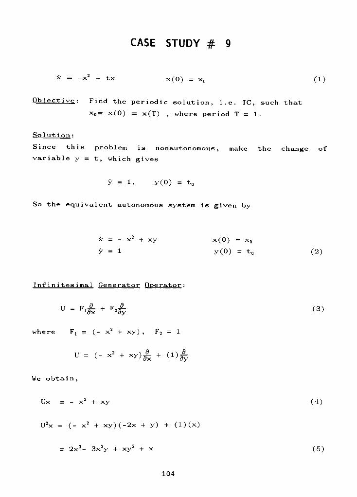
CASE STUDY # 9

X = + txx(0) =

x0 (1)

Objective: Find the periodic solution, i.e. IC, such that

x0=x(0) =

x(T) , where period T = 1.

Solut ion :

Since this problem is nonautonomous, make the change of

variable y = t, which gives

y = 1, y(0) = t0

So the equivalent autonomous system is given by

x = -

x2

+ xy x(0) = x0

y = 1 y(0) = t0 (2)

Infinites imal Generator Operator :

U =

F +F4 (3)

where Fx = (- x2

+ xy) , F2 = 1

U = (- x2

+ xy)A + (1)

We obtain ,

Ux = -

x2

+ xy (4)

U2x = (- x2

+ xy)(-2x + y) + (l)(x)

= 2x3- 3x2y +xy2

+ x (5)

104

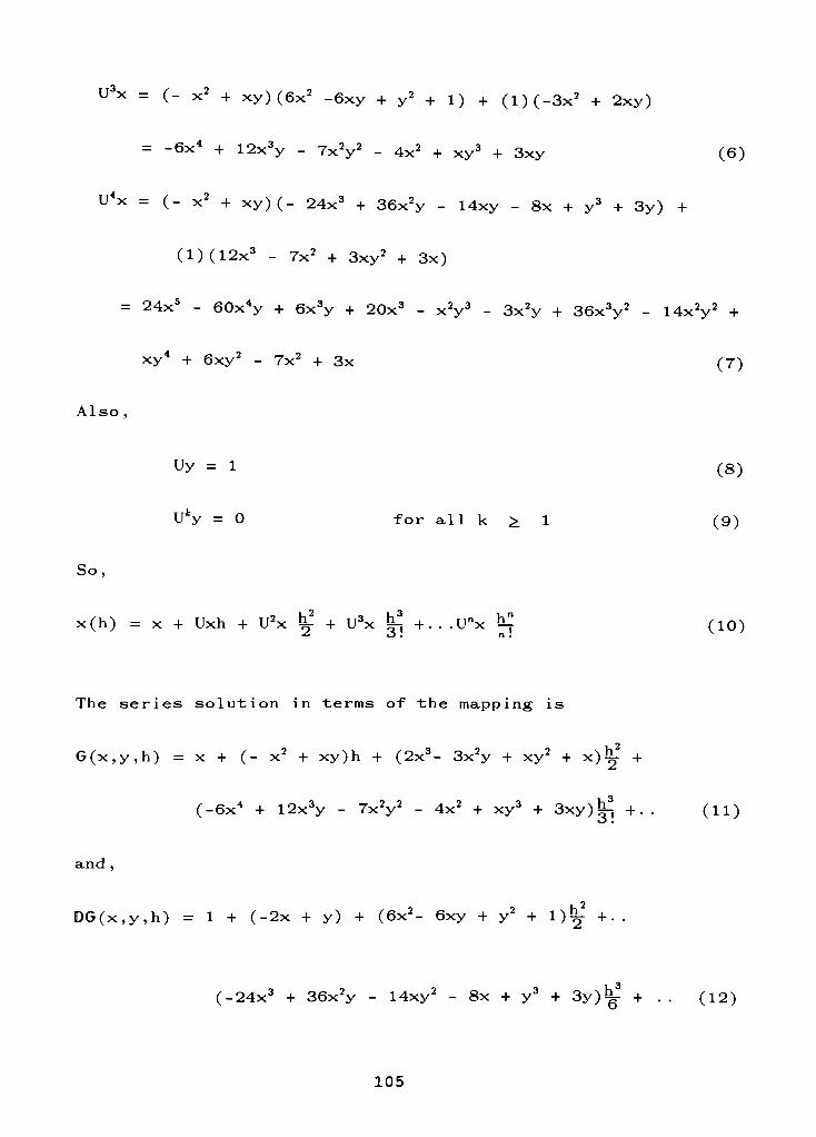
U3x = (- x2

+xy)(6x2

-6xy +y2

+ 1) +(l)(-3x2

+ 2xy)

= + 12x3y -

7x2y2-

4x2

+xy3

+ 3xy (6)

U4x = (- x2

+ xy)(- 24x3

+ 36x2y - 14xy - 8x +y3

+ 3y) +

(l)(12x3-

7x2

+3xy2

+ 3x)

=24x5

- 60x4y + 6x3y +20x3

-

x2y3

- 3x2y +36x3y2

-

14x2y2

+

xy4

+6xy2

-

7x2

+ 3x (7)

Also,

Uy = 1(8)

U*y = 0 for all k ^ 1 (9)

So,

x(h) = x + Uxh -)- U2x ^ + U3x ^ +. . .Unx ^ (10)

The series solution in terms of the mapping is

G(x,y,h) = x + (- x2

+ xy)h + (2x3- 3x2y +xy2

+x)^

+

(-6x4

+ 12x3y -

7x2y2-

4x2

+xy3

+ 3xy)^ + . . (11)

and,

DG(x,y,h) = 1 + (-2x + y) + (6x2- 6xy +y2

+ !)% +..

(-24x3

+ 36x2y -

14xy2- 8x +

y3

+ 3y)^ + .. (12)

105

Equations (11) and (12) are entered into the Fortran progr

TEST. FOR with period T=l, and the fixed point was found to be

am

x0 = 0.5428

The following plot verifies that the above value is a periodic

solution .

106

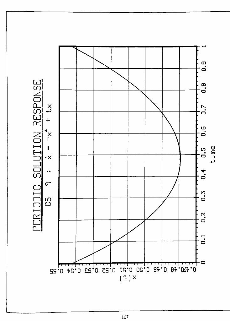
. en

"o

LJ

CO

O

CL

CO

LJ

en

oi i

t-

ZD

_J

O

CO

X

-p

+

X

1

1

X

. oo

70

70

. LO

0.->

-P

0

CDi i

Q

Oi i

en

LJ

CL

or

co

CJ

. to

0

- CM

O

J

O

O

!SS"

0*s*

0S*

0SS1

1 1 1 1

0IS-

0OS'

0 6K 0 8VQtt'O

107

CASE STUDY # 10

x -I-

sin(x) = sin(2*-t) (1)

Qb ]ect ive : Find the periodic solution of the above equation,

such that x0=x(0) = x(T) ,

where the period = 2ir .

Solut ion :

Since equation (1) is nonautonomous, it can be re-expressed as

an autonomous one by letting x =xx ,

and t = x2 . Equation (1)

can be written as

= -

sin(xx) + sin(2?rx2) (2)

equation (2) can now be replaced by two first order

differential equations

Xj = -

sin(Xi) + sin(2?rx3) xx(0) = xl0

x2= t x2(0) = t0

The series solution in terms of a mapping was calculated from

the program VECFLD2 with the information F1 = -

sin(xt) +

sin(2?rx2) and F2 = 1 entered, and stored in the following

subprograms

Xl(h)= G1(-Kl,-x.2,h)

- subprogram [ gnnxh.for]

108

gx-(x1,x2,h)-

subprogram [dgnnxh.for]

The above subprograms are called by the main Fortran program

TEST. FOR to solve for the periodic solution value, with period

T = 2ic . Because of the nonlinearity of the system for this

problem, more than one periodic solution was found

x0 = - 0.1553, 2.9863, 6.1279, 9.2695,

which are incremented by the value ir . Plots are displayed in

the graphs that follow to verify the periodic solution found.

Copies of all the programs used for the calculation are located

in Appendix A.

109

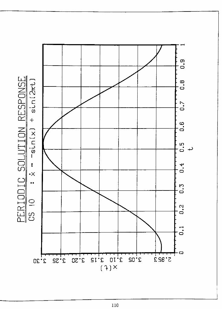
LJ r-^

CO -P

OX

CL_ c

CO -_>

LJCO

en +

~ZL ^

oX

1 1c

E-h-_>

ID CO

_J

1

O n

COX

o1 1

o

ni i o

en

LJ CO

CL CJ

; -p

0' Sc*" 0S" SI" OI'E S0* S6'Z

no

CASE STUDY # 11

-

x = + sin(t) x(0) = x0 (1)

Objective : Find the periodic solution, i.e. IC, such that

x0=x(0) =

x(T) , where period T = 2n -

Solution :

Since this problem is nonautonomous, make the change of

variable y = t, which gives

y = 1, y(0) = t0

So the equivalent autonomous system is given by

x = -

x3

+ sin(t) x(0) = x0

y = i y(o)= t0 (2)

The series expansion was found to be from the program VECFLD2

to be

G(x,y,h) = x + (- x3

+ sint)h + (3x5- 3x2sint + cost)|- +

(-15x7+ 21x4sint -

6x(sint)2- 3x2cost

-sint)^-f . . . (3)

and,

DG(x,y,h) = 1 - 3x2h + (15x4- 6x sint )^ +(-105x6

+ 84x3sint -

6(sint)2-6xcost)|- + . . . (4)

Equations (3) and (4) are entered into two subprograms, and are

used by the main Fortran program TEST . FOR to solve for the

111

fixed point (periodic solution) with period T=2t . The periodic

value was found to be

x0 = - 0.71576

The above point was plotted to verify that it is a periodic

solution. The graph of this value is on the following page.

Also, copies of all computer programs used are in Appendix A.

The problem was resolved with the damping term reduced to

0.1,

O.lx3

+ sin(t) x(0) = x0 (5)

The new periodic solution value was identified as

x0= - 0.9988

The graph for this new damping is displayed on the second plot

112

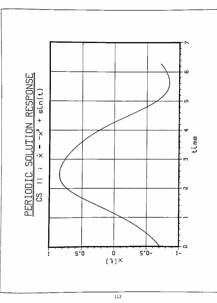
LJ

CO^

o H->

CL

00 c

LJ.p

COen

+~7*

oX

1 1I

M

ID 1

_J

OX

CO*

o1 1

~~~~

CD

CDi CO

enCJ

LJ

CL.

\

;

I S"l3 0S"

3- I

CO

m

CD

-P

to

r\j

CU*

113

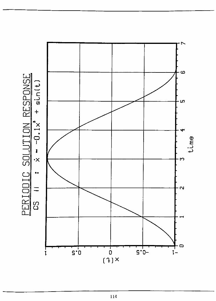
LJ

CO

O

CL

CO

LJ

en

CDi i

E-

O

CO

O

CD

O

en

LJ

cl

c-P

CO

I

X

COCJ

mx

114

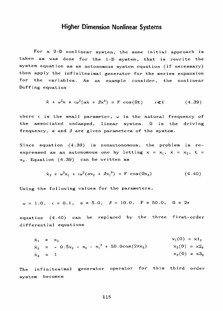
Higher Dimension Nonlinear Systems

For a 2-D nonlinear system, the same initial approach is

taken as was done for the 1-D system, that is rewrite the

system equation as an autonomous system equation (if necessary)

then apply the infinitesimal generator for the series expansion

for the variables. As an example consider, the nonlinear

Duffing equation

x + w2x + ew2(ax + /?x3) = F cos(ftt) <1 (4.39)

where e is the small parameter, u is the natural frequency of

the associated undamped, linear system. ft is the driving

frequency, a and /? are given parameters of the system.

Since equation (4.39) is nonautonomous, the problem is re-

expressed as an autonomous one by letting x =xt , x = x2 ,

t =

x3 . Equation (4.39) can be written as

x2 + w2xx + ew2(ax2 + /?xx3) = F cos(ftx3) (4.40)

Using the following values for the parameters,

u = 1.0, e = 0.1, a = 5.0, /? = 10.0, F = 50.0, ft = 2tt

equation (4.40) can be replaced by the three first-order

differential equations

-l= x2 xx(0) =

xl0

x2= - 0.5x2

-

xx-

Xi3

+ 50.0cos(2ttx3) x2(0) =x20

x3= 1 x3(0) =

x30

The infinitesimal generator operator for this third order

system becomes

115

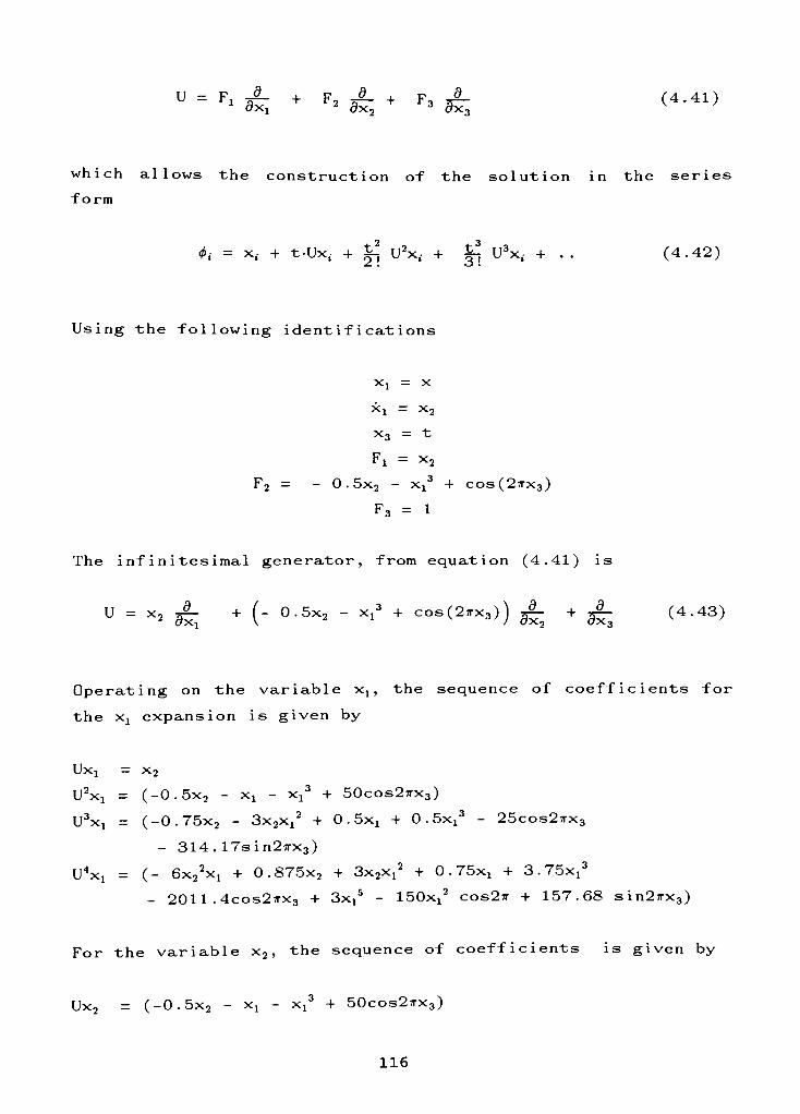
U =

F'A + *iir+ F*si <4-41)

which allows the construction of the solution in the series

form

<t>i = x,. + tUx, + |^U2x,- + |^ U3x,- + .. (4.42)

Using the following identifications

x, = x

xi x2

F1 =x2

F2 = - 0.5x2 -

xx3

+ cos(2irx3)

F3 = 1

The infinitesimal generator, from equation (4.41) is

u = x2 A + (_ -5x2 _

Xj3

+cos^2'rx3>) A + A (4-43)

Operating on the variable xx ,the sequence of coefficients for

the Xi expansion is given by

Ux: = x2

U2Xi = (-0.5x2 -

xx-

xx3

+ 50cos2:rx3)

U3xx = (-0.75x2 -

3x2X!2

+ 0.5xi + 0 .

5xx3- 25cos27rx3

- 314.17sin2;rx3)

U4Xl = (- 6x22Xl + 0.875x2 +3x2Xl2

+ 0 . 75x: + 3 .

75xx3

- 2011 .4cos2?rx3 +3x!5

-

150x!2

cos2?r + 157.68 sin2:rx3)

For the variable x2 ,the sequence of coefficients is given by

Ux2 = (-0.5x2 -

xx-

Xi3

+ 50cos2ttx3)

116

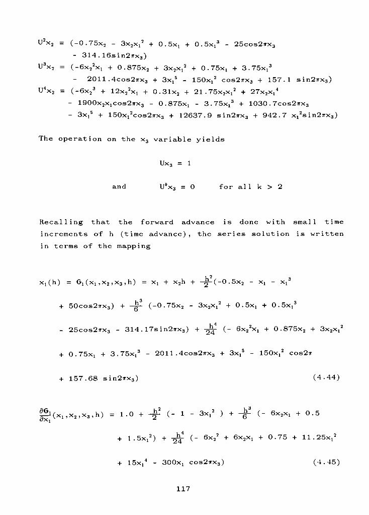
U2x2 = (-0.75x2 -

3x2Xl2

+ 0.5xx +0.5xj3

- 25cos27rx3

- 314. 16sin27rx3)

U3x2 = (-6x22Xl + 0.875x2 +3x2xj2

+ 0 . 75xj + 3 .

75xt3

2011.4cos2jtx3 +

3xx5-

150x!2

cos2ix3 + 157.1 sin2ix3)

U4x2 =(-6x23

+ 12x22Xl + 0.31x2 +21.75x2Xl2

+27x2Xl4

-

1900x3X^032^X3 -

0.875X! -

3.75xx3

+ 1030 . 7cos2?rx3

-

3xx5

+ 150x12cos2irx3 + 12637.9 sin2:rx3 + 942.7 x12sin2irx3)

The operation on the x3 variable yields

Ux3 = 1

and U*x3 = 0 for al 1 k > 2

Recalling that the forward advance is done with small time

increments of h (time advance), the series solution is written

in terms of the mapping

.23

xj(h)= G1(x1,x2,x3,h) =

xx + x2h + -^-(-O.Sxj-

xx-

xx

+ 50cos25rx3) + -g1- (-0.75x2 -

3x2Xi2

+ 0 . 5xx + 0 .

5xx3

- 25cos2ttx3- 314.17sin27rx3) +

-^(- 6x22X! + 0.875x2 +

3x2Xl2

+ 0.75xt +3.75X!3

- 2011 .4cos2ttx3 +3xx5

-

150x!2

cos2tt

+ 157.68 sin27rx3) (4.44)

^(Xi.xj.xa.h) = 1.0 +-^

(- 1 -

3xx2

) +-^

(- 6x2xx + 0.5

h_ (_ v.2j. fiv.v. -1- n 7K 4- 11 OSv.2

+ 1.5xt2) +2^

("6x2J

+ 6x2Xl + 0.75 +11.25Xl2

+ 15X/- 300xx cos2ttx3) (4.45)

117

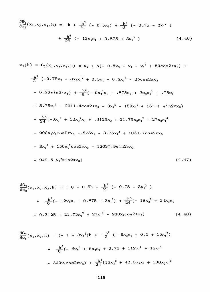
^(x1,x2,x3,h) = h +-^

(_o.5x2) +

-^(- 0.75 -

3xx2

+ tjj- (-12x2Xl + 0.875 +

3xx2

) (4.46)

x2(h) = G2(x1,x2,x3,h) =x2 + h(- 0 . 5x2 -

xx-

xt3

+ 50cos2ttx3) +

-^-

(-0.75x2 -

3x2xj2

+ 0.5xj +0.5x!3

- 25cos2ix3

-

6.28sin27rx3) + -|p(- 6x22Xj + .875x2 +3x2X!2

+ . 75xj

+3.75x!3

- 2011.4cos27rx3 +

3Xi5-

150x!2

+ 157.1 sin2irx3)

+^(-6x23

+ 12x22Xl +.3125x2 +

21.75x2X!2

+27x2X!4

- 900x2x1cos2ttx3 -

. 875xx - 3 .

75xj3

+ 1030 . 7cos27rx3

-

3xj5

+ 150x12cos2ttx3 + 12637 . 9s in25rx3

+ 942.5 x12sin25rx3) (4.47)

aG2/- -- --

h) = 1.0 - 0.5h + -Jjf " ^c " 2

+ -y-(- 12x2Xi + 0.875 + 3xt2) + -^i.~18x22

+ 24x2Xl

^(Xl,x2,x3,h) = 1.0 - 0.5h + -%- (- 0.75 - 3x/ )

h3- -

^4

+ 0.3125 +21.75xx2

+27xx4

- 900xlCos27rx3) (4.48)

^(Xl,x2,h) = (- 1 - 3xx2)h +-

(- 6x2xx + 0.5 + 15xx2)CXi

-I- -4p(-

6x22

+ 6x2xj + 0.75 +112xi2

+15xx4

- 300x1cos2?rx3) + + 43.5x2Xl +108x2Xl3

118

-

900x2cos27rx3 -.875-

11.625X!2-

15xj4

+ 300XJCOS2TX3

+ 1184.9 xlSin2irx3) (4.49)

For a 2-D system the algorithm for finding the solution is

modified slightly from that used for a 1-D system, due to the

presence of matrix operations. Recalling that for the system

we deduce G(x) , and then P(x) = Gn(x) ,the fixed point is equal

to the Poincare mapping of the initial condition

x0 = P(x0) (4.50)

To find the initial condition that leads to a fixed point, we

will need P(x) and P (x) and use Newton-Raphson to iterate

until the fixed point is located (if it exists). The

calculation of P(x) = G(G ( . . . G(x) ) . . . ) ,now involves matrix

man i pu 1at i ons .

Jacobian of the Compos ite Mapping ;

P(x) = G(G(. . .G(x)). ..) (4.51)

First, consider the composition of vector functions:

Let yx= f1(x1,x2, .

.xm)

y2= "f2(xi,X2, .

.Xm)

ym = fm(Xj,X2, ..xm)

y = f (x)

vector function

fromRm

toRm

119

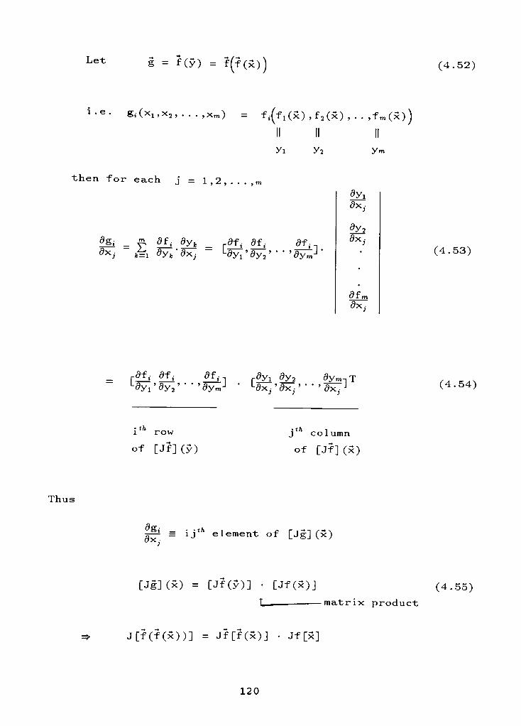
Letg = f (y) =

f(f(x)) (4.52)

i-e-S,(x1,x2,...,Xm) =

f,(f1(x),f2(x),..,fm(x))

yi y2 ym

then for each j = 1,2,.

dgi= ^ <H\ dy,

_ 5^ df. df

d*j *=i dyk*

d^j~

LdYl'

ay2' * *

' 5y^J*

yi

dx,

dy2<9x.

dfm

fcc,

(4.53)

Sf, df, 5f^L5yi'5y2" '<9ymJ

r^yi dy2 5ym-,T

Lax>'aX;. ' ' 5Xj. J (4.54)

i1*

row

of [Jf](y)

j column

of [Jf](x)

Thus

|ji =ij"1

element of [Jg] (x)

[Jg](x) = [Jf(y)] [Jf(x)j (4.55)

L -matrix product

J[*Cf(x))] = Jf [f(x)J Jf [x]

120

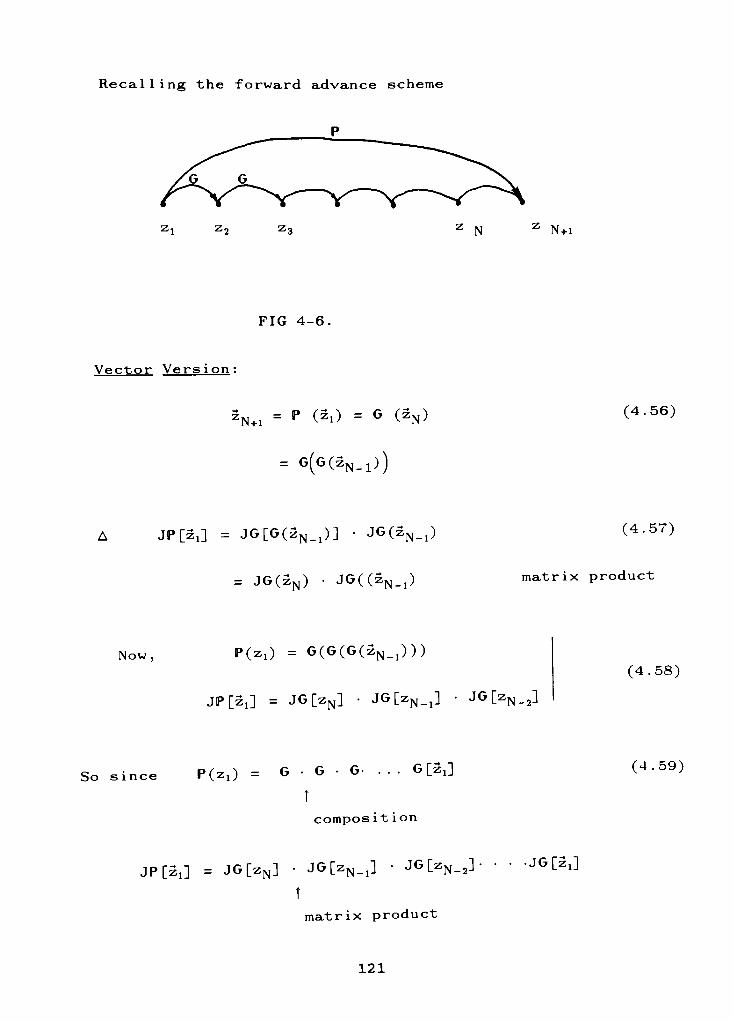
Recalling the forward advance scheme

z, z, zN

zN+i

FIG 4-6

Vector Version :

Wi = p <2i> = G (2n)

=

G(G(2N-1>)

(4.56)

A JP[2J = JG[G(zN_x)] JG(2N_0 (4.57)

= JG(zN) JG((zN-1)matrix product

Now, P(zi) = G(G(G(Zn_x)))

jp[z1] = JG[zN] JG[zN_J JG[zN_2]

(4.58)

So since >(Zl) = G G G-. . G[z:]

T

compos it ion

jpr^] = JG[zN] JG[zN_t]JG[zN_2]-

-JG[2X]

(4.59)

matrixproduct

121

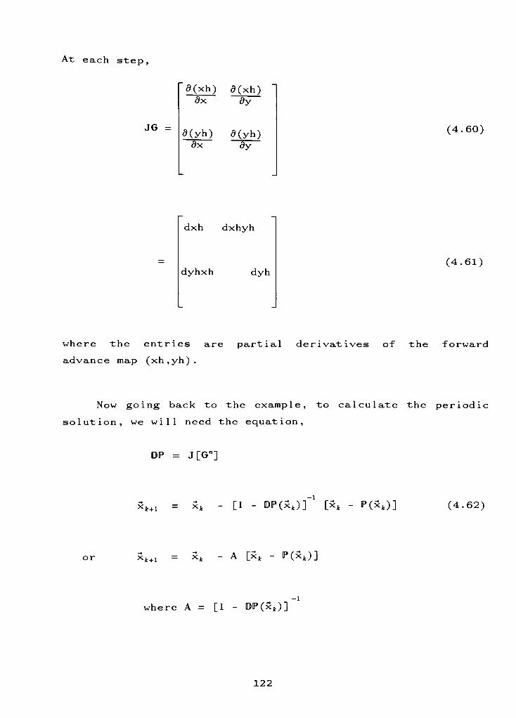
At each step,

JG =

fl(xh) 9(xh)ax ay

g(yh) fl(yh)ax ay

(4.60)

dxh dxhyh

dyhxh dyh(4.61)

where the entries are partial derivatives of the forward

advance map (xh,yh) .

Now going back to the example, to calculate the periodic

solution, we will need the equation,

DP = J[G"]

Xfc+1= xt

- [I - 0P(xJ] [xt - P(xt)]X (4.62)

or xt+1= xt

- A [xt - P(xt)]

where A = [I - DP(xt)]

122

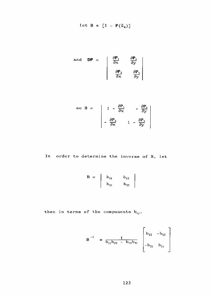
let B = [I -

P(xt)]

and DP =a_Pjax

ap_2ax

aPjdy

ap,ay

so B = 1 -

ap,

dP1ax

ax1 -

a_Pi

ay

ap,

ay

In order to determine the inverse of B, let

B = bll b12

b21 b22

then in terms of the components bi; ,

Bbllb22 ~ b12b

21

b22 ~b12

-b21 bll

123

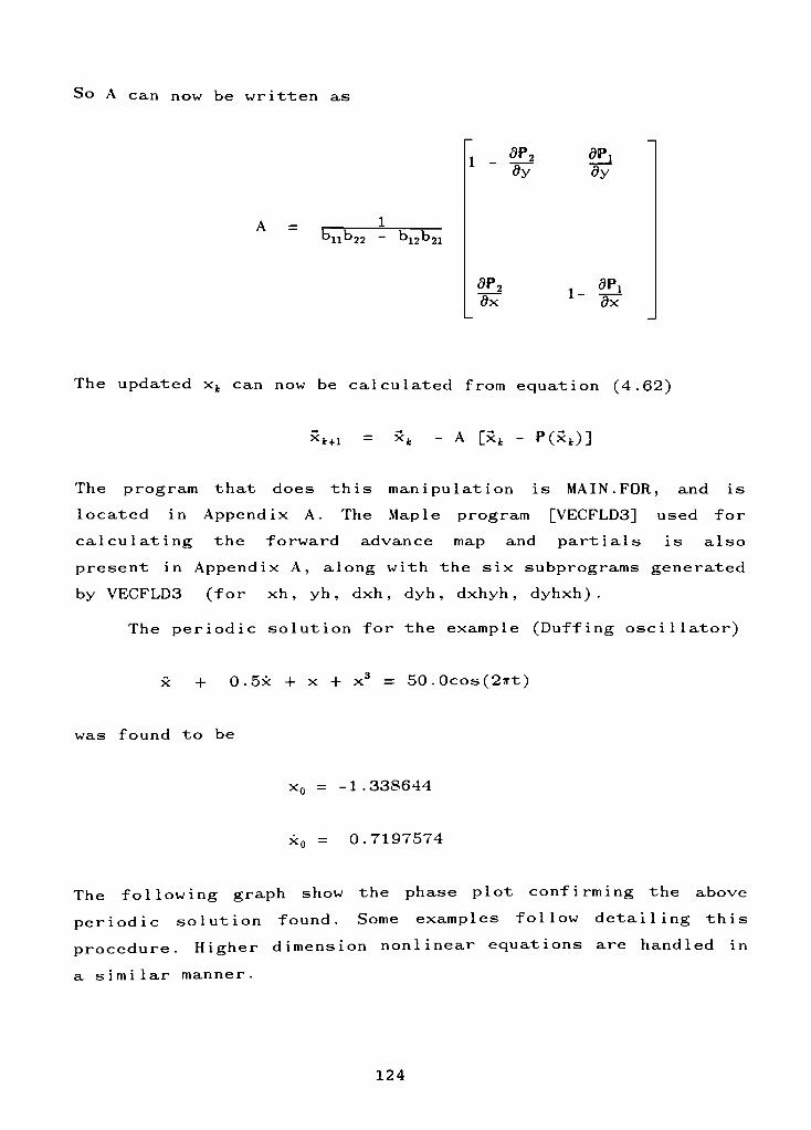
So A can now be written as

A =

bllb22 b,,b12u21

ap,

ay

ap_2ax

dP1

dy

a_Piax

The updated xt can now be calculated from equation (4.62)

"*+i- A [xt - P(xt)]

The program that does this manipulation is MAIN. FOR, and is

located in Appendix A. The Maple program [VECFLD3] used for

calculating the forward advance map and partials is also

present in Appendix A, along with the six subprograms generated

by VECFLD3 (for xh ,yh

,dxh

,dyh

,dxhyh

, dyhxh) .

The periodic solution for the example (Duffing oscillator)

x + 0.5x + x +x3

= 50.0cos(27rt)

was found to be

xn = -1.338644

xf = 0.7197574

The following graph show the phase plot confirming the above

periodic solution found. Some examples follow detailing this

procedure. Higher dimension nonlinear equations are handled in

a similar manner.

124

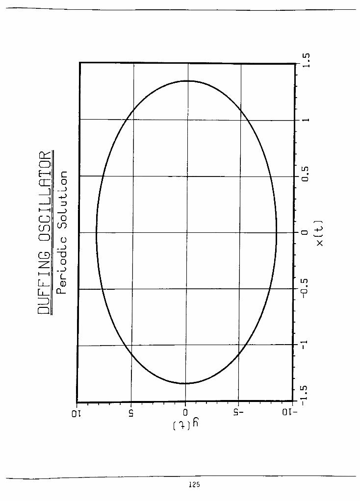
en

CDt-i c

en o

_j

-P

i i )

C") o

COCO

o o

._)

CD "O

~z.o

1 1t_

L_ CD

L_ Q_

ZD

CD

-P

X

125

CASE STUDY # 12

x -

a(l - x2)x + x = F sin(ftt) (1)

Ob iect ive : Find the periodic solution of the above Vanderpol

equation, such that x0= x(0)= x(T),

where the period ft = 2w .

Solut ion :

Since equation (1) is nonautonomous, it can be re-expressed as

an autonomous one by letting x = x1 ,x = x2 and t = x3 . Equation

(1) can be written as

x2- a(l -

xx2)x2 + xt= F sin(ftx3) (2)

Using the following values for the parameters,

a = 0.2, ft = 2;r,

F = 50

equation (2) can now be replaced by three first order

differential equations

:x= x2 *i(0) =

xl0

c2= -

Xl- 0.2(Xl2)x2 + 0.2x2 + F sin(fix3) x2(0) =

x20

:3= 1 x3(0) =

x30

The series solution in terms of a mapping was calculated from

the program VECFLD3 with the information Fx = x2 , F2 =x2 and F3

= 1 entered, and stored in the following subprograms

126

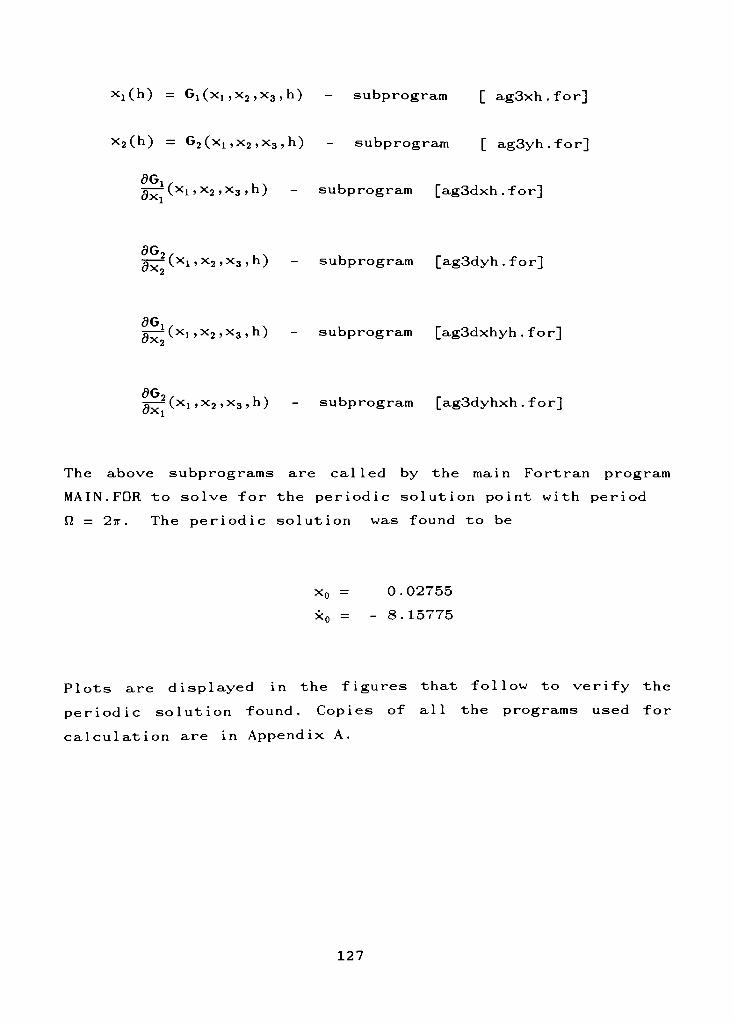
xi(h) = G^x^XjjXajh) -

subprogram [ ag3xh.for]

x2(h) = G2(xl5x2 ,x3 ,h) -

subprogram [ ag3yh.for]

Op

3^~(xi ?x2 5X3 ,h)-

subprogram [ag3dxh.for]

op

^^(xi ,x2 ,x3,h)-

subprogram [ag3dyh.for]

g^i(xi,x2,x3,h)- subprogram [ag3dxhyh .for]

o- (xt ,x2 ,x3 , h) - subprogram [ag3dyhxh .

f"

or]CXi

The above subprograms are called by the main Fortran program

MAIN. FOR to solve for the periodic solution point with period

ft = 2tt . The periodic solution was found to be

x0 = 0.02755

x = - 8.15775

Plots are displayed in the figures that follow to verify the

periodic solution found. Copies of all the programs used for

calculation are in Appendix A.

127

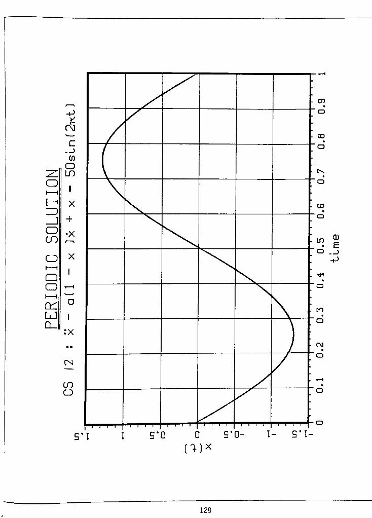
mx

128

129

o

ZD

O

CO

CDi i

Q

O

-P

J?c-.J

CO

o

LO

1

X

+

X

X

en

LJ

CL

:x

-P

o

CD

co

o

_c

Q_

"D

CD

O

D

"D

0

en

^ 01

co

o

130

CONCLUSIONS and RECOMMENDATIONS

The technique developed in this investigation can be used

to locate periodic solutions for forced linear and nonlinear

systems. The technique is semi -automated by the use of MAPLE

(symbolic mathematics program). Symbolic computation allows for

efficient manipulation of differential equations and initial

conditions, leading to periodic solutions. For linear systems,

as well as nonlinear systems, a MAPLE program algorithm was

developed to generate Infinitesimal Generator series expansions

of the solutions. These solutions were easily converted to

Fortran code (as subroutines) by MAPLE and easily called by the

main Fortran program for the determination of initial

conditions which give rise to periodic solutions. Although

attention has been given to the solution of first and second

order equations, the technique can easily be extended to

higher-order equations, as pointed out in the respective

"developmentsections"

for linear and nonlinear systems.

Steady state solutions were analyzed by utilizing the

associatedPoincare'

Mapping of flow. It was shown that

periodic solutions of dynamical systems correspond to fixed

points of the time-advance mapping. For linear systems, the

Poincare'

Map can in principle be explicitly determined. This

is based on the fact that forced solutions can be developed

from the fundamental solutions of the system. For first-order

systems, this turns out to be an elementary exercise. For

higher order systems, the explicit calculations can be

formidable. The proposed method is efficient to use and does

not compromise any accuracy for stable linear systems.

ThePoincare'

map for a nonlinear system cannot in general

be analyticallyderived. This would require solution of the

governingequations. Instead, series approximations were

developed, based on Lie Series expansions. These solutions were

only approximate, but the ability to symbolically compute the

131

series expansions out to an arbitrary number of terms allows

for highly accurate analytical expressions for thePoincare'

map. Even the brute-force method is only an approximation. When

the algorithm converges, it does offer a highly efficient way

of finding periodic solutions that would otherwise be based on

trial and error.

For nonlinear systems, the one drawback of the proposed

methodology is that the initial guess required to start the

Newton-Raphson iteration must be in the basin of attraction of

the periodic solution (if it exists). Otherwise, the algorithm

will not converge due to instabilities or the presence

competing basins of attraction.

Recommendations for the extension of this work include

modification of the programs to allow reverse mapping (that is,

backward time stepping) . Such a procedure could be used to

locate periodic solutions that are unstable under a positive

time advance. Perhaps a global search method could be developed

which would seek out all fixed points of thePoincare'

map in a

specified region of state space. Indeed, some nonlinear systems

support multiple or even an infinite number of periodic

solutions. As a final recommendation, the computer codes could

be modified to enable computation of the eigenvalues of the

Poincare'map. These associated eigenvalues measure the orbital

stability characteristics of periodic solutions.

132

REFERENCES

1- P. Hagedorn, Nonl inear Qsc i I 1 at ions. Clarendon Press,Oxford (1981).

2. L. Meirovitch, Analytical Methods in Vibrations.Macm i 1 1 an

, Toronto ( 1 967) .

3. T.J. Aprille, Jr and T.N. Trick, "A Computer Algorithmto Determine the Steady-State Response of Nonlinear

Oscillators", IEEE Transactions on Circuit Theory. Vol

CT-19, No. 4, pp. 354-360 (July 1972).

4. T.S. Parker and L.O. Chua, "The Double Scroll Equation",IEEE Transactions on Circuits and Systems. Vol CAS-34,pp. 1059-1073 (September 1987).

5. T.J. Aprille, Jr and T.N. Trick, "Steady State Analysisof Nonlinear Circuits with Periodic Inputs", Proceedings

of the IEEE, Vol 60, No. 1 (January 1972).

6. N. Minorsky, Nonl inear Osci 1 lat ions . Nostrand, PrincetonNew Jersey (1962) .

7. E.R. Rainville and P.E. Bedient, Elementary Differential

Equat ions . Macmillan, New York.

8. J.S. Torok and S.H. Advani, "Continuous Transformation

Groups and Series Solution of Initial Value Problems",Int. J . Non-Linear Mech . . Vol 20,No. 4, pp. 283-289

(1985) .

9. Maple - Symbolic Computation Program

10. J.R. Ward and R.D. Strum, State Variable Analysis .

Prentice-Hall, Englewood Cliffs, New Jersey (1970).

11. J.S. Torok, "Symbolic Computation of Lie Series for the

Solution of Ordinary Differential Equations", Proceedings .

1991 ASEE Annual Conference, New Orleans.

12. A. Cohen, An Introduct ion to the Lie Theory of

One -Parameter Groups , D.C. Heath, Boston (1911).

13. P. Tondeur, Introduct ion to Lie Groups and Transformat i on

Groups . Springer-Valley, Berlin (1969).

14. G.M. Swisher, Introduct ion to Li near Systems Analvs is .

Matrix Publishers, Inc., Oregon (1976).

133

APPENDIX A

134

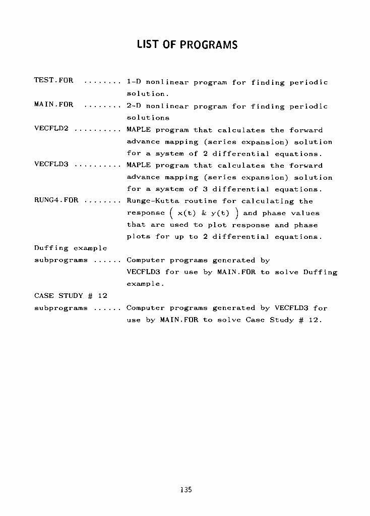
LIST OF PROGRAMS

lEbl . rUR 1-D nonl inear program for finding periodic

solution .

MAIN. FOR 2-D nonlinear program for finding periodic

solut ions

VECFLD2 MAPLE program that calculates the forward

advance mapping (series expansion) solution

for a system of 2 differential equations.

VECFLD3 MAPLE program that calculates the forward

advance mapping (series expansion) solution

for a system of 3 differential equations.

RUNG4.F0R Runge-Kutta routine for calculating the

response ( x(t) k y(t) J and phase values

that are used to plot response and phase

plots for up to 2 differential equations.

Duffing example

subprograms Computer programs generated by

VECFLD3 for use by MAIN. FOR to solve Duffing

example .

CASE STUDY #12

subprograms Computer programs generated by VECFLD3 for

use by MAIN. FOR to solve Case Study # 12.

135

* *

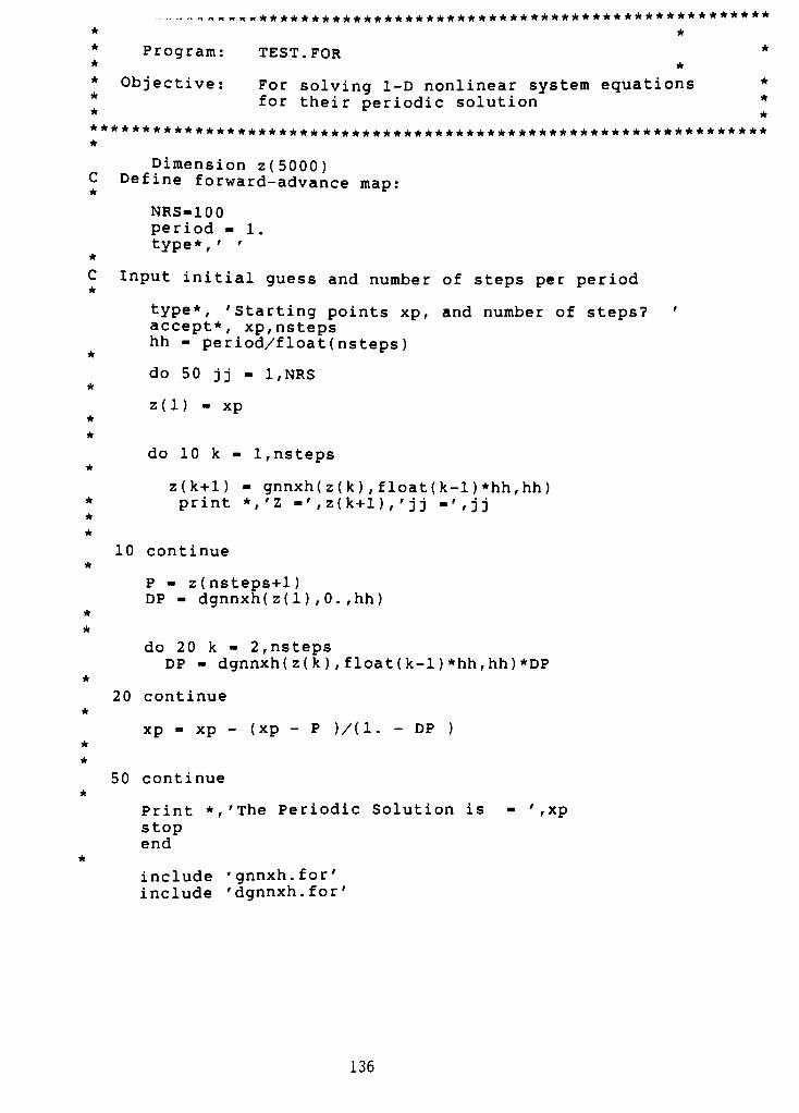
*Program: TEST. FOR

*

* *

*Objective: For solving 1-D nonlinear system equations

*

for their periodic solution*

* *

*

Dimension z(5000)C Define forward-advance map:

NRS-100

period - 1.type*

,

' '

C Input initial guess and number of steps per period

type*, 'Starting points xp, and number of steps?'

accept*, xp,nsteps

hh -

period/float(nsteps)

do 50 jj - 1,NRS

z( 1) - xp

*

*

*

*

*

do 10 k - l,nsteps

z(k+l) - gnnxh(z(k) , f loat( k-l ) *hh,hh)print *,'Z

'

,z(k+l) ,

'

jj ',jj

10 continue

P - z(nsteps+l)

DP - dgnnxh( z(l ) ,0. ,hh)

do 20 k - 2,nsteps

DP - dgnnxh(z(k) , float ( k-l ) *hh, hh) *DP

20 continue

xp-

xp- (xp

- P )/(l. - DP )

50 continue

Print *,'The Periodic Solution is - ',xp

stopend

include'gnnxh.for'

include'dgnnxh.for'

136

c

*PROGRAM: MAIN. FOR *

**

*OBJECTIVE: THIS PROGRAM SOLVES 2-D NONLINEAR EQUATIONS FOR *

PERIODIC SOLUTIONS.*

i *

#

Parameter NP-2

^

Dimension x( 5000 ) ,y( 5000 ) ,A(np,np) ,D( np,np) ,B(np,np)

C Define forward-advance map:

period - 1.type*,' '

C Input initial guess and number of steps per period

type*, 'Starting points xp, yp and number of steps, and NRS?

accept*, xp,yp,nsteps,NRShh -

period/float(nsteps)

do 500 jj - 1,NRS

x( 1) - xp

yd) -

yp

do 5 k - l,nsteps

x(k+l) -

aG3xh(x(k),y(k),float(k-l)*hh,hh)y(k+l) -

aG3yh(x(k),y(k),float(k-l)*hh,hh)C print*, x(k+l) ,y(k+l)

5 continue

DP1X - ag3dxh(x(l) ,y( 1 ) , 0 . 0,hh)DP1Y -

ag3dxhyh(x(l),y(l),0.0,hh)

DP2X - ag3dyhxh(x(l) ,y( 1 ) , 0 . 0 ,hh)

DP2Y - ag3dyh(x(l),y(l),0.0,hh)

Do 10 k-2,nsteps

DNP1X - ag3dxh(x(k) ,y(k) , float( k-l ) *hh,hh)DNP1Y - ag3dxhyh(x(k) ,y(k) , float ( k-l ) *hh,hh)DNP2X - ag3dyhxh(x(k) ,y(k) , float ( k-l ) *hh,hh)

DNP2Y - ag3dyh(x(k) ,y( k ) , float( k-l ) *hh,hh)

P1X - DNP1X*DP1X + DNP1Y*DP2X

PlY - DNP1X*DP1Y + DNP1Y*DP2Y

P2X - DNP2X*DP1X + DNP2Y*DP2X

P2Y - DNP2X*DP1Y + DNP2Y*DP2Y

DP1X - P1X

DP1Y - PlY

DP2X - P2X

DP2Y - P2Y

10 Continue

C Set up Matrix B

137

B(l,l) - 1.0-DP1XB(l,2) -

-DP1Y

B(2,l) --DP2X

B(2,2) - 1.0-DP2Y

*Compute B inverse

B1-1.0/(B(1,1)*B(2,2) - B(1,2)*B(2,1))

D(l,l) -

B(2,2)D(l,2) -

-B(l,2)

D(2,l) -

-B(2,l)

D(2,2) - B(l,l)

Do 11 I-l,npDo 12 J-l,np

A(I,J) -B1*D(I,J)

12 Continue

11 Continue

C

C Print *,((A(i,j), j-l,np),i-l,np)c

c

diffx -

xp-

x(nsteps+l)

diffy -

yp-

y(nsteps+l)

xp -

xp-

A(l,l)*diffx-A(l,2)*diffyyp

-

yp-

A(2,l)*diffx-A(2,2)*diffy

500 continue

Print *,'The Periodic Solution is - '/Xp, yp

stopend

Subprograms called

function ag3xh( xl ,x2,x3 ,h)

include 'ag3xh.for'

return

end

function ag3dxh( xl ,x2 ,x3 ,h)

include 'ag3dxh.for'

return

end

function ag3yh( xl ,x2 ,x3 ,h)

include 'ag3yh.for'

return

end

function ag3dyh(xl,x2,x3,h)

138

include 'ag3dyh.for'

return

end

functionag3dxhyh(xl,x2,x3,h)

include 'ag3dxhyh. for '

return

end

function ag3dyhxh(xl ,x2,x3 ,h)include 'ag3dyhxh. for '

return

end

139

# Program VECFLD2# This code computes the Nth order series approximation of the

# solution to a system of 2 first order differential equations,

# The time advance variable is denoted by h.

#

with( linalg ) :

# Define the right hand side of the equation.

#

Fl :0.1*xl~3+sin(x2) ;F2 :- 1;

#

vars :- [xl ,x2] :

#

vec :- array( [ F1,F2] ) :w :- array( [ xl,x2 ] ) :

#

xh :- xl:

yh :- x2:

#

for k from 1 to N do

J :- jacobian(w, vars) :

#

Uw :- evalm( J&*vec ) :

#

xh :- xh + Uw(l]*(h~k)/factorial(k) t

yh :- yh + Uw[ 2 ] *(h~k )/factorial( k) :

w : - Uw :

od:

# Print the Nth order series approximation

#

xh;

yh;

F:-proc(a,b)

subs(xl-a,x2-b,xh) :

end:

G:-proc( a ,b)

subs ( xl-a,x2-b,yh) :

end:

#

dxh:-dif f (xh,xl) :

readlib( fortran) :

xhl :-evalf (xh) :

dxhl:-evalf (dxh) :

fort ran (xhl, f ilename-'gxh. for'optimized) :

fortran(dxhl,filename-,dgxh.for,

optimized) :

140

#

#

#

#

#

with

#

#Fl

F2

F3

#

Program VECFLD3This code computes the Nth order series approximation of

the solution to a system of 3 first order differentialequations. The time advance variable is denoted by h.

( 1 inalg) :

Define the right hand side of the equation.

= x2;

= 1;

1 . 0*xl+ .2*x2-

. 2*xl *x2+50*s i n (6 . 28315*x3) ;

: = [xl,x2,x3]

vars

#vec :=

array ( [Fl , F2 , F3] ) :

w :=array ( [xl ,x2,x3] ) :

#

xh : = xl :

yh : = x2:

zh : = x3:

#for k from

J

#1 1

#

u

1 to N do

:= jacobian(w,vars)

' :=evalm(Jt*vec) :

xh

yh

zh

Print the Nth order series approximation

:= xh + Uw[l]*(h~k) /factorial (k):= yh + Uw[2]*(h"k)/factorial (k):= zh + Uw[3]*(h"k)/factorial (k)

od :

#

#xh ;

yh;

zh ;

#dxh:=diff (xh,xl) :

dyh:=diff (yh,x2) :

dxhyh:=diff (xh,x2) :

dyhxh:=diff (yh,xl) :

readl ib(fortran) :

dxhyhl : =evalf (dxhyh) :

dyhxhl : =evalf (dyhxh) :

xhl :=evalf (xh) :

dxhl :=evalf (dxh) :

yhl :=evalf (yh) :

dyhl :=evalf (dyh) :

fort ran (xhl ,f ilename='

ag3xh .

for'

,opt imized) :

fort ran (dxhl ,f ilename='

ag3dxh , optimized) :

fort ran (yhl,f ilename='

ag3yh , optimized) :

fort ran (dyhl ,f ilename='

ag3dyh .

for'

,opt imized) :

fort ran (dxhyhl ,f ilename='

ag3dxhyh .

for'

,opt imized)

fort ran (dyhxhl , f ilename='

ag3dyhxh .

for'

,opt imized)

#

141

**************************************************

*

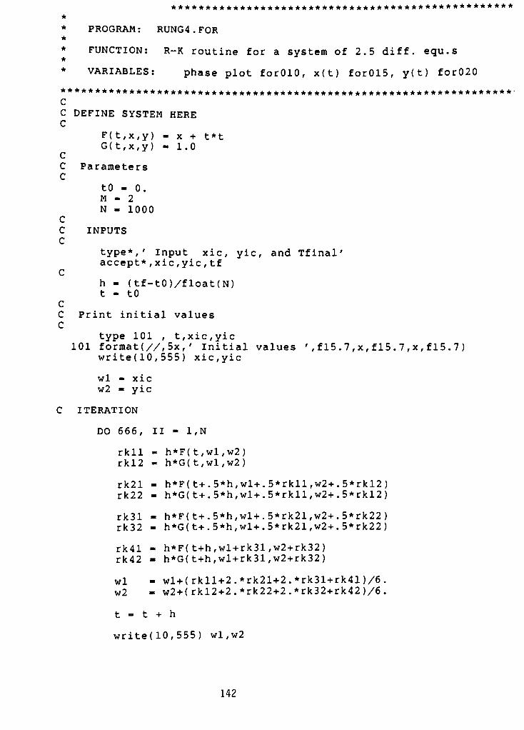
* PROGRAM: RUNG4 . FOR*

* FUNCTION: R-K routine for a system of 2.5 diff. equ.s

*

* VARIABLES: phase plot forOlO, x(t) for015, y(t) for020

?j****************************************************************-

C

C DEFINE SYSTEM HERE

C

F(t,x,y) - x + t*t

G(t,x,y) - 1.0C

C Parameters

C

to - 0.

M - 2

N - 1000

C

C INPUTS

Ctype*,'

Input xic, yic, andTfinal'

accept*, xic, yic, tf

C

h - (tf-t0)/float(N)t - to

C

C Print initial values

C

type 101 , t, xic, yic

101 format(//,5x,'Initial values

'

, f15 . 7 ,x, f15. 7 ,x, f15 . 7 )wri te( 10 , 555 ) xic, yic

wl - xic

w2 - yic

C ITERATION

DO 666, II - 1,N

rkll - h*F(t,wl,w2)

rkl2 - h*G(t,wl,w2)

rk21 - h*F(t+.5*h,wl+.5*rkll,w2+.5*rkl2)

rk22 - h*G( t+.5*h,wl+.5*rkll,w2+.5*rkl2)

rk31 - h*F( t+. 5*h,wl+.5*rk21,w2+.5*rk22 )

rk32 - h*G( t+ . 5*h,wl+ . 5*rk21 ,w2+ . 5*rk22 )

rk41 - h*F( t+h,wl+rk31,w2+rk32)

rk42 - h*G( t+h,wl+rk31 , w2+rk32 )

wl - wl+(rkll+2.*rk21+2.*rk31+rk41)/6.

w2 = w2+( rkl2+2.*rk22+2.*rk32+rk42)/6.

t - t + h

write(10,555) wl,w2

142

write(15,555) t,wl

write(20,555) t,w2

555 Format(5x,fl5.7,5x,fl5.7)

666 Continue

STOP

END

143

Programs generated by VECFLD3 and used for the Duffing example

calculat ion

g3xh.for [Xi(h)]

g3yh.for [x2(h)J

g3dxh.for [|^(xl5x2,x3,h)]Sxj

d!T2

gSdxhyh.for [|gl(Xl,x2,x3,h)]

gSdyh.for [^(xl5x2,x3,h)]

-^xV-^l > -*-2 -*-3 :

g3dyhxh.for [^(Xl,X25X3)h)]

144

g3xh .for

t4 xl**2

t5 = t4*xl

t7 - 0.628315El*x3t8 -

cos(t7)

til - h**2

tl5 - x2*t4

t20 - sin(t7)

t26 - x2**2

t34 - t4**2

t41 - tll**2

t44 - xl+x2*h+0.5E0*(-0.5E0*x2-xl-t5+50.0*t8)*tll+0.1666667E0*(-0.

+7 5E0*x2-3.0*tl5+0.5E0*xl+0.5E0*t5-0.25E2*t8-0.3141575E3*t20)*tll*h

++0.4166667E-l*(-6.0*t26*xl+0.87 5E0*x2+0.3El*tl5+0.75E0*xl+0.375El*

+t5-0.2011399E4*t8+3.0*t34*xl-150.0*t4*t8+0.1570788E3*t20)*t41

g3xh - t44

145

g3yh .for

t3 - xl**2

t4 - t3*xl

t6 - 0.628315El*x3t7 -

cos(t6)

tl2 - x2*t3

tl7 -

sin(t6)

t20 - h**2

t23 - x2**2

t24 - t23*xl

t31 - t3**2

t32 - t31*xl

t34 - t3*t7

t62 - t20**2

t65 - x2+(-0.5E0*x2-xl-t4+50.0*t7)*h+0.5E0*(-0.75E0*x2-3.0*tl2+0.5

+E0*xl+0.5E0*t4-0.25E2*t7-0.3141575E3*tl7)*t20+0.1666667E0*(-6.0*t2

+4+0.87 5EO*x2+0.3El*tl2+0.75EO*xl+0.375El*t4-0.2011399E4*t7+3.0*t32

+-150.0*t34+0.1570788E3*tl7)*t20*h+0.4166667E-l*(-6.0*t23*x2+0.12E2

+*t2 4+0.312 5E0*x2+0.2175E2*tl2+27.0*x2*t31-900.0*x2*xl*t7-0.87 5E0*x

+1-0. 387 5E1 *t4+0. 1030699E4*t7-0.3El*t32+0.15E3*t34+0. 126 3792E5*tl7+

+0.9424725E3*t3*tl7)*t62

g3yh - t65

146

g3dxh .for

tl = xl**2

t4 - h**2

t7 - x2*xl

tl4 - x2**2

tl8 - tl**2

t25 - t4**2

t28 - 1.0+0

+*tl)*t4*h+0

+tl8-300

g3dxh -

5EO*(-1.0-3.0*tl)*t4+0.1666667EO*(-6.0*t7+0.5EO+0.15El4166667E-l*(-6.0*tl4+0.6El*t7+0.75EO+0.1125E2*tl+15.0*

0*xl*cos(0. 62831 5El*x3) )*t25t28

147

g3dyh.for

t2 - xl**2

t5 - h**2

t8 - x2*xl

tl5 - x2**2

tl9 - t2**2

t26 - t5**2

t29 - 1.0-0.5EO*h+0.5EO*(-0.75EO-3.0*t2)*t5+0.1666667EO*(-12.0*t8+

+0.875E0+0.3El*t2)*t5*h+0.4166667E-l*(-18.0*tl5+0.24E2*t8+0.3125E0+

+0.2175E2*t2+27.0*tl9-900.0*xl*cos(0.628315El*x3) )*t26

g3dyh - t29

148

g3dxhyh.for

tl - h**2t3 =

xl**2

tl3 - tl**2

+-12 n*v;S-?5^0o^+-1666667E0*(-0-75E0-3-0*t3)*tl*h+0.4166667E-l*(+-12.0*x2*xl+0.87 5EO+0.3El*t3)*tl3g3dxhyh - tl6

149

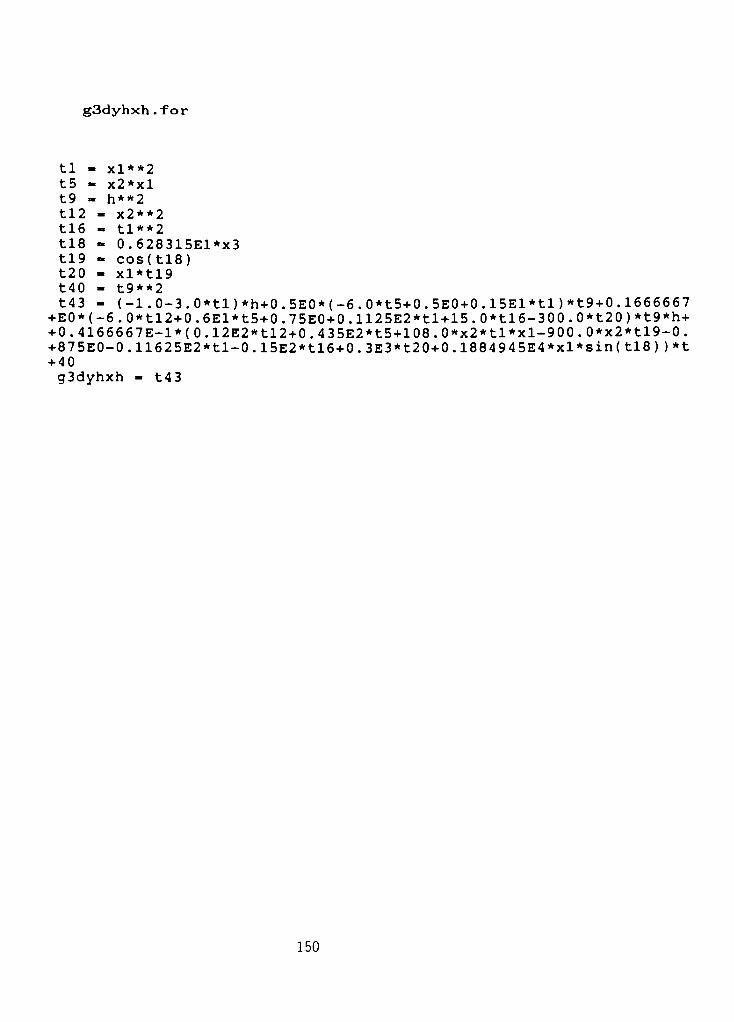
g3dyhxh . for

tl - xl**2

t5 - x2*xl

t9 - h**2

tl2 - x2**2

tl6 - tl**2

tl8 - 0.628315El*x3

tl9 -

cos(tl8)

t20 - xl*tl9

t40 - t9**2

t4 3 - (-1.0-3.0*tl)*h+0.5E0*(-6.0*t5+0.5E0+0.15El*tl)*t9+0.1666667

+E0*(-6.0*tl2+0.6El*t5+0.75E0+0.1125E2*tl+15.0*tl6-300.0*t20)*t9*h+

+0.4166667E-l*(0.12E2*tl2+0.4 3 5E2*t5+108.0*x2*tl*xl-900.0*x2*tl9-0.

+87 5E0-0.11625E2*tl-0.15E2*tl6+0.3E3*t20+0.1884 94 5E4*xl*sin(tl8) )*t

+ 40

g3dyhxh - t43

150

Programs generated by VECFLD3 and used for Case Study # 12

ca 1 cu 1at ion

ag3xh.for IX (h)]

ag3yh.for [x2(h)]

ag3dxh.for [^(Xi ,x2 ,x3 ,h)]

ag3dyh.for [_J(Xl ,x2 ,x3 , h)]-5x

2

AC

ag3dxhyh.for [^ (Xi ,x2 ,x3 , h) ]^2

AC

ag3dyhxh.for [^ (xj ,x2 ,x3 , h) ]

151

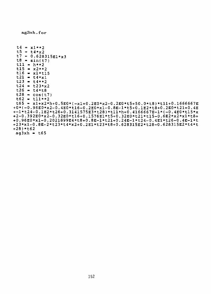
ag3xh . for

t4 - xl**2

t5 - t4*x2

t7 = 0.628315El*x3t8 -

sin(t7)til - h**2

tl5 - x2**2

tl6 - xl*tl5

t21 - t4*xl

t23 - t4**2

t24 - t23*x2

t26 - t4*t8

t28 - cos(t7)

t62 - tll**2

t6 5 - xl+x2*h+0.5E0*(-xl+0.2E0*x2-0.2E0*t5+50.0*t8)*tll+0.1666667E

+0*(-0.96E0*x2-0.4E0*tl6-0.2E0*xl-0.8E-l*t5+0.lE2*t8+0.2E0*t21+0.4E

+-l*t24-0.lE2*t26+0.3141575E3*t28)*tll*h+0.4166667E-l*(-0.4E0*tl5*x

+2-0.392E0*x2-0.32E0*tl6+0.1576El*t5+0.32E0*t21*tl5-0.6E2*x2*xl*t8+

+0.96E0*xl-0.2021899E4*t8+0.8E-l*t21+0.24E-l*t24-0.4El*t26-0.4E-l*t

+23*xl-0.8E-2*t23*t4*x2+0.2El*t23*t8+0.628315E2*t28-0.628315E2*t4*t

+28)*t62

ag3xh - t65

152

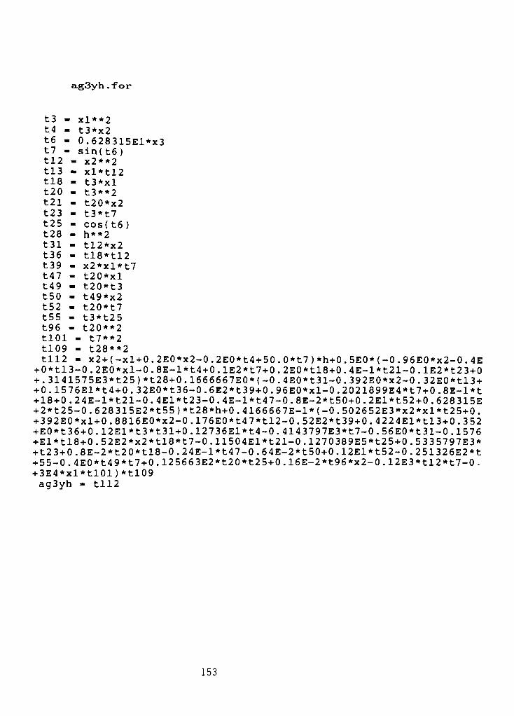
ag3yh .for

t3 - xl**2

t4 - t3*x2

t6 - 0.628315El*x3t7 -

sin(t6)tl2 - x2**2

tl3 - xl*tl2

tl8 - t3*xl

t20 - t3**2

t21 - t20*x2

t23 - t3*t7

t25 -

cos(t6)

t28 - h**2

t31 - tl2*x2

t36 - tl8*tl2

t39 - x2*xl*t7

t47 - t20*xl

t49 - t20*t3

t50 - t49*x2

t52 - t20*t7

t55 - t3*t25

t96 - t20**2

tlOl - t7**2

tl09 - t28**2

til 2 - x2+(-xl+0.2E0*x2-0.2E0*t4+50.0*t7)*h+0.5E0*(-0.96E0*x2-0.4E

+0*tl3-0.2E0*xl-0.8E-l*t4+0.lE2*t7+0.2E0*tl8+0.4E-l*t21-0.lE2*t2 3+0

+.3141575E3*t25)*t28+0.1666667E0*(-0.4E0*t31-0.392E0*x2-0.32E0*tl3+

+0.1576El*t4+0. 32E0*t36-0. 6E2*t39+0. 96E0*xl-0.2021899E4*t7+0.8E-l*t

+18+0. 24E-1 *t21-0.4El*t23-0. 4E-l*t47-0.8E-2*t50+0.2El*t 52+0. 628 31 5E

+2*t2 5-0.628 315E2*t55)*t28*h+0.4166667E-l*(-0.502652E3*x2*xl*t25+0.

+392E0*xl+0.8816E0*x2-0.176E0*t47*tl2-0.52E2*t39+0.4224El*tl3+0.3 52

+E0*t36+0.12El*t3*t31+0.12736El*t4-0.4143797E3*t7-0.56E0*t31-0.1576

+El*tl8+0.52E2*x2*tl8*t7-0.1150 4El*t21-0.1270389E5*t2 5+0.53 3 5797E3*

+t2 3+0.8E-2*t20*tl8-0.24E-l*t47-0.64E-2*t50+0.12El*t52-0.251326E2*t

+55-0.4E0*t49*t7+0.12 566 3E2*t2 0*t25+0.16E-2*t96*x2-0.12E3*tl2*t7-0-

+3E4*xl*tl01)*tl09

ag3yh - tll2

153

ag3dxh .for

tl - xl*x2

t4 - h**2

t7 - x2**2

tlO - xl**2

tl2 - tlO*xl

tl3 - tl2*x2

tl5 - 0.628315El*x3

tl6 -

sin(tl5)

tl7 - xl*tl6

t33 - tl0**2

t45 - t4**2

t48 -1.0+0.5E0*(-0.lEl-0.4E0*tl)*t4+0.1666667E0*(-0.4E0*t7-0.2E0-

+0. 16E0 * 1 1 +0. 6E0 * tl 0+0. 16E0 * tl 3-0. 2E2*tl7)*t4*h+0. 416666 7E-1*( -0.32

+E0*t7+0.3152El*tl+0.96E0*tl0*t7-0.6E2*x2*tl6+0.96E0+0.24E0*tl0+0.9

+6E-l*tl3-0.8El*tl7-0.2E0*t33-0.48E-l*t33*xl*x2+0.8El*tl2*tl6-0.125

+66 3E3*xl*cos( tl5) )*t45

ag3dxh - t48

154

ag3dyh .for

tl - xl**2

t5 - xl*x2

t8 - tl**2

til - h**2

tl4 - x2**2

tl8 - tl*xl

tl9 - tl8*x2

t21 - 0.628315El*x3

t22 - sin(t21)

t23 - xl*t22

t26 - t8*tl

t50 - t8**2

t56 - tll**2

t59 - 1.0+(0.2E0-0.2E0*tl)*h+0.5E0*(-0.96E0-0.8E0*t5-0.8E-l*tl+0.4

+E-l*t8)*tll+0.1666667E0*(-0.12El*tl4-0.392E0-0.64E0*t5+0.1576El*tl

++0.6 4EO*tl9-0.6E2*t2 3+0.24E-l*t8-0.8E-2*t26)*tll*h+0.4166667E-l*(-

+0.52E2*t23+0.52E2*tl8*t22+0.12736El*tl+0.8816E0+0.8448El*t5-0.1150

+4El*t8+0.704E0*tl9-0.6 4E-2*t26-0.168El*tl4-0.5026 52E3*xl*cos(t21)+

+0.36El*tl*tl4-0.3 52E0*t8*xl*x2+0.16E-2*t50-0.24E3*x2*t22)*t56

ag3dyh - t59

155

ag3dxhyh .for

tl - xl**2

t4 - h**2

t7 - xl*x2

tlO - tl**2

tl6 - x2**2

t31 - t4**2

t34 - h+0.5E0*(0.2E0-0.2E0*tl)*t4+0.1666667E0*(-0.96E0-0.8E0*t7-0.+8E-l*tl+0.4E-l*tlO)*t4*h+0.4166667E-l*(-0.12El*tl6-0.392EO-0.64EO*

+t7+0.1576El*tl+0.6 4E0*tl*xl*x2-0.6E2*xl*sin(0.628315El*x3)+0.24E-l+*tlO-0.8E-2*tlO*tl)*t31ag3dxhyh - t34

156

ag3dyhxh . for

tl - xl*x2

t5 - x2**2

t8 - xl**2

tlO - t8*xl

til - tl0*x2

tl3 - 0.628315El*x3tl4 -

sin(tl3)

tl5 - xl*tl4

tl8 - h**2

t23 - t8*t5

t25 - x2*tl4

t31 - t8**2

t33 - t31*xl

t34 - t33*x2

t36 - tl0*tl4

t38 - cos(tl3)

t39 - xl*t38

t76 - tl4**2

t83 - tl8**2

t86 - (-0.lEl-0.4E0*tl)*h+0.5E0*(-0.4E0*t5-0.2E0-0.16E0*tl+0.6E0*t

+8+0.16E0*tll-0.2E2*tl5)*tl8+0.1666667E0*(-0.32E0*t5+0.3152El*tl+0.

+96E0*t23-0.6E2*t25+0.96E0+0.24E0*t8+0.96E-l*tll-0.8El*tl5-0.2E0*t3

+1-0. 48E-l*t34+0.8El*t36-0. 12 566 3E3*t39 ) *tl8*h+0 .4166667E-1* ( -0 . 52E

+2*t2 5-0.502652E2*t39+0.156E3*x2*t8*tl4+0.502652E2*tlO*t38+0.2 54 72E

+1 *tl+0.392E0+0.1 0671 59E4*tl 5+0. 4224El*t5-0. 46016El*tl1-0. 4728El*t8

++0. 1 0 56E1 * t2 3-0. 38 4E-1 *t34+0. 48El*t36-0. 12E0*t31-0. 5026 52E3*x2*t 38++0.56E-l*t31*t8+0.24El*xl*t5*x2-0.88E0*t31*t5+0.128E-l*t31*tl0*x2-

+0.3E4*t76-0.24El*t33*tl4)*t83

ag3dyhxh - t86

157