Stats Lunch: Day 4

Intro to the General Linear Model and Its Many, Many

Wonders, Including:

T-Tests

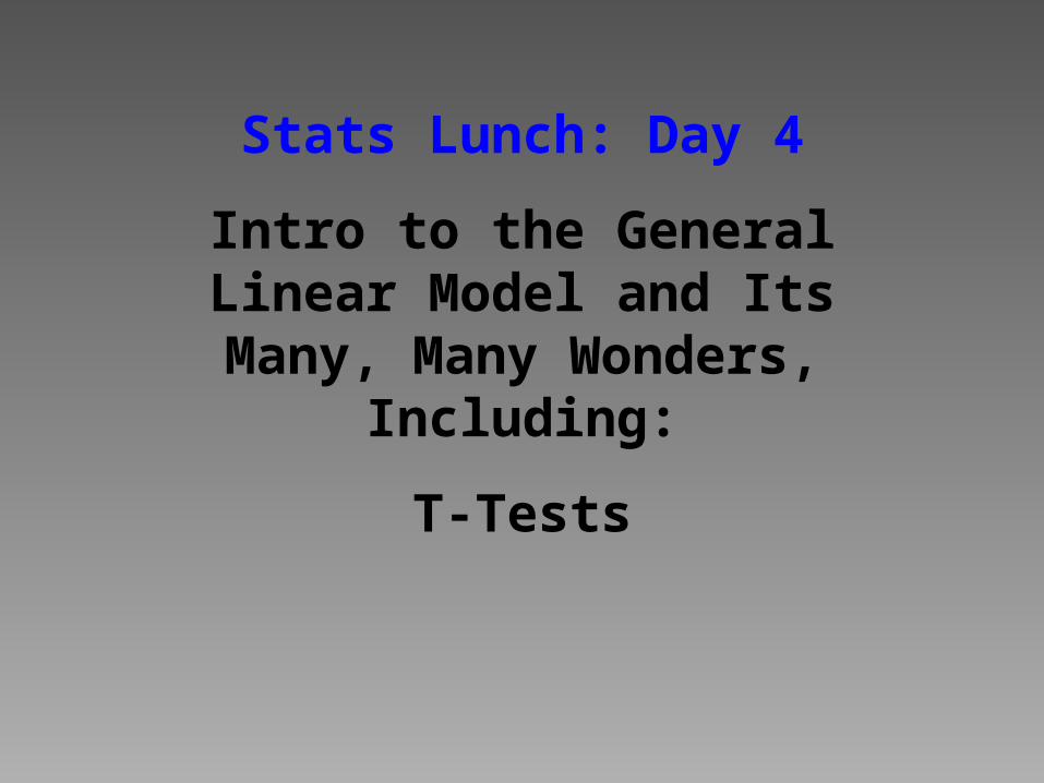
Steps of Hypothesis Testing

1. Restate your question as a research hypothesis and a null hypothesis about the populations

2. Determine the characteristics of the comparison distribution (mean and standard error of sampling distribution of the means)

3. Determine the cutoff sample score on the comparison distribution at which the null hypothesis could be rejected

4. Determine your sample’s score on the comparison distribution

5. Decide whether to reject the null hypothesis

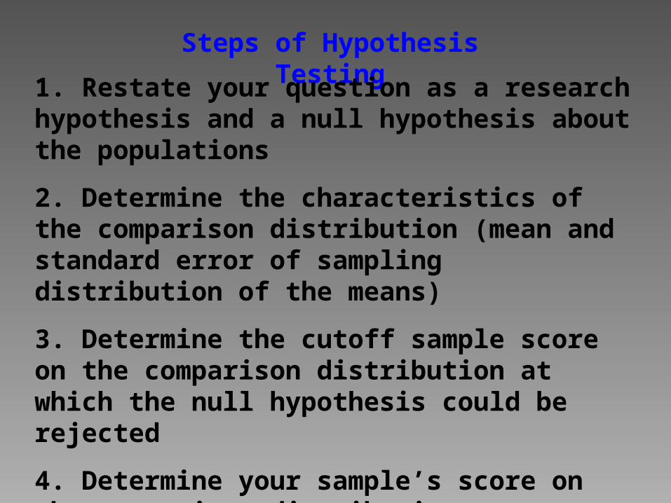
The General Linear Model

Mathematical Statement expressing that the score of any participant in a treatment condition is the linear sum of the population parameters.

Yij = T + i + ij

Individual Score Grand Mean Treatment Effect

Experimental Error

Basic Assumptions of the GLM

1) Scores are independent.

2) Scores in treatment populations are (approximately) normally distributed.

3) Variance of scores in treatment populations are (approximately) equal.

The General Linear Model

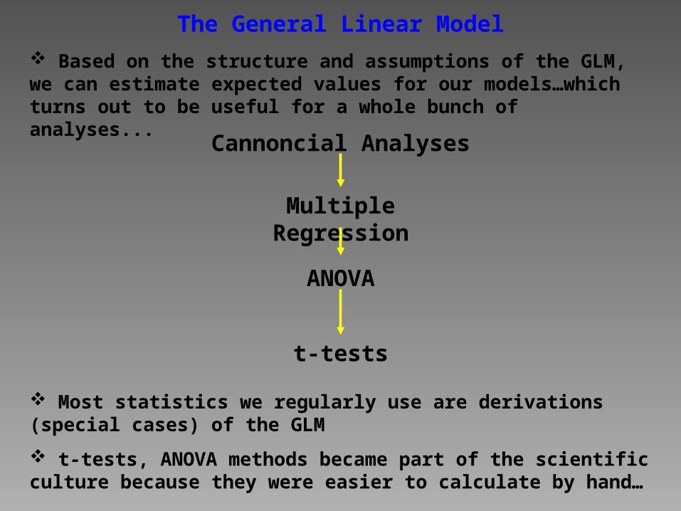
Based on the structure and assumptions of the GLM, we can estimate expected values for our models…which turns out to be useful for a whole bunch of analyses...

Cannoncial Analyses

Multiple Regression

ANOVA

t-tests

Most statistics we regularly use are derivations (special cases) of the GLM

t-tests, ANOVA methods became part of the scientific culture because they were easier to calculate by hand…

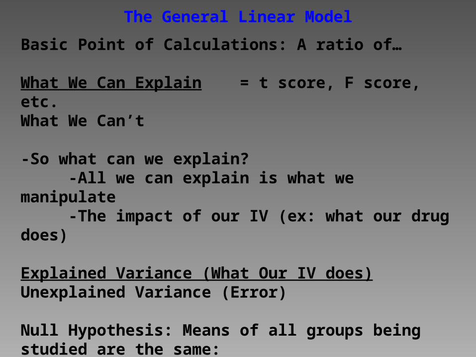
Basic Point of Calculations: A ratio of…

What We Can Explain = t score, F score, etc.What We Can’t

-So what can we explain?-All we can explain is what we manipulate-The impact of our IV (ex: what our drug does)

Explained Variance (What Our IV does)Unexplained Variance (Error)

Null Hypothesis: Means of all groups being studied are the same:-Mean Old Drug = Mean New Drug = Mean Placebo

The General Linear Model

The General Linear Model

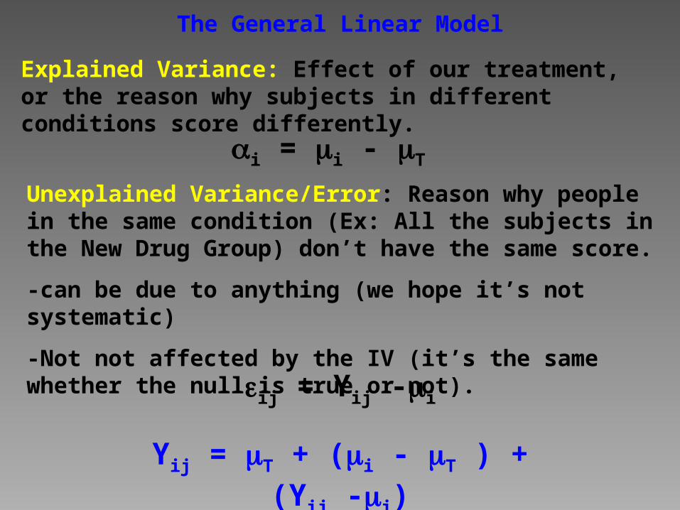
Explained Variance: Effect of our treatment, or the reason why subjects in different conditions score differently.

i = i - T

Unexplained Variance/Error: Reason why people in the same condition (Ex: All the subjects in the New Drug Group) don’t have the same score.

-can be due to anything (we hope it’s not systematic)

-Not not affected by the IV (it’s the same whether the null is true or not).

ij = Yij -i

Yij = T + (i - T ) + (Yij -i)

W.S. Gosset and the t-test

Gosset was employed by the Guinness brewery to scientifically examine beer making.

Due to costs, only had access to small samples of ingredients.

Needed to determine the probability of events occurring in a population based on these small samples.

Developed a method to estimate PARAMETERS based on SAMPLE STATISTICS.

These estimates varied according to sample size (t-curves)

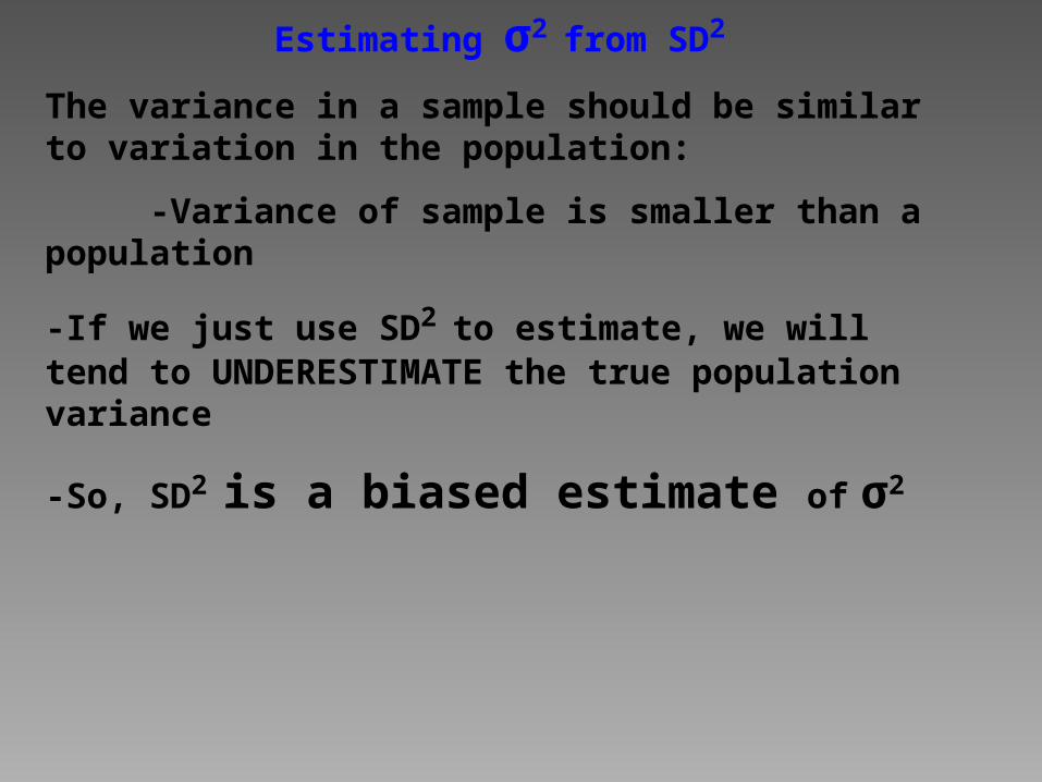
Estimating σ2 from SD2

The variance in a sample should be similar to variation in the population:

-Variance of sample is smaller than a population

-If we just use SD2 to estimate, we will tend to UNDERESTIMATE the true population variance

-So, SD2 is a biased estimate of σ2

-How far off our guess is tied to the # of subjects we have...

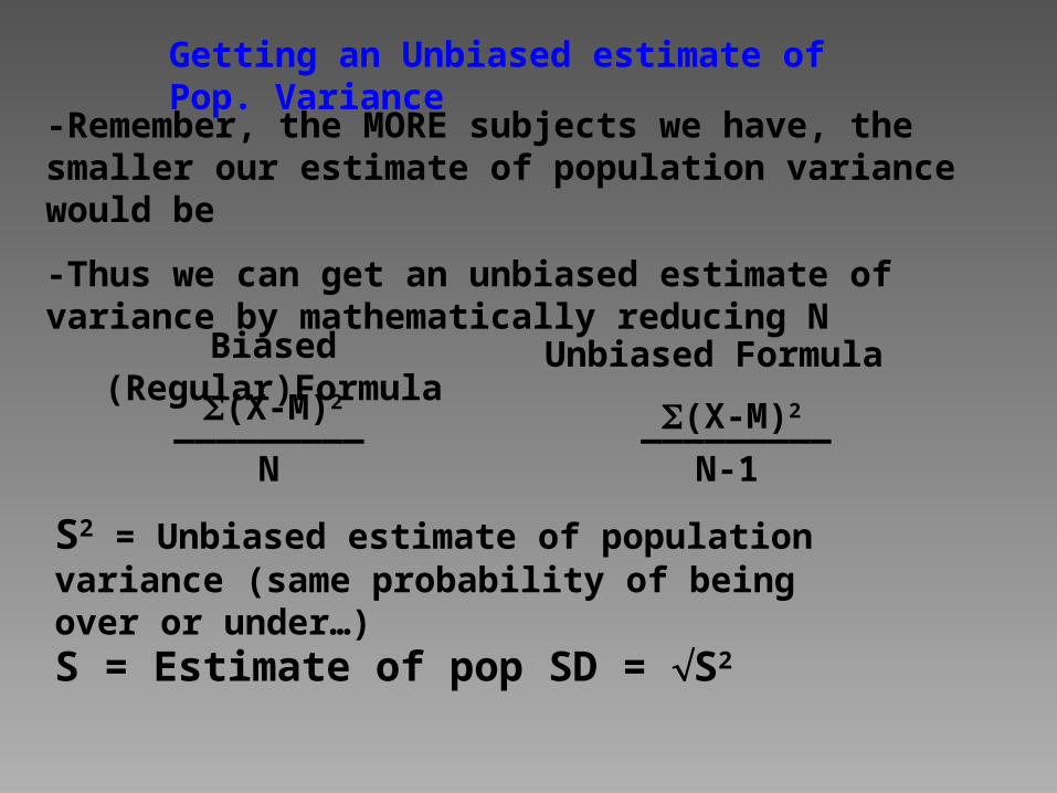
Getting an Unbiased estimate of Pop. Variance

-Remember, the MORE subjects we have, the smaller our estimate of population variance would be

-Thus we can get an unbiased estimate of variance by mathematically reducing N

Biased (Regular)Formula Unbiased Formula

(X-M)2_________

N_________(X-M)2

N-1

S2 = Unbiased estimate of population variance (same probability of being over or under…)

S = Estimate of pop SD = S2

_________(X-M)2

N-1

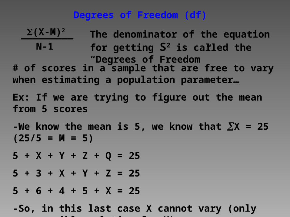
Degrees of Freedom (df)

The denominator of the equation for getting S2 is called the “Degrees of Freedom”

# of scores in a sample that are free to vary when estimating a population parameter…

Ex: If we are trying to figure out the mean from 5 scores

-We know the mean is 5, we know that X = 25 (25/5 = M = 5)

5 + X + Y + Z + Q = 25

5 + 3 + X + Y + Z = 25

5 + 6 + 4 + 5 + X = 25

-So, in this last case X cannot vary (only one possible solution for X)

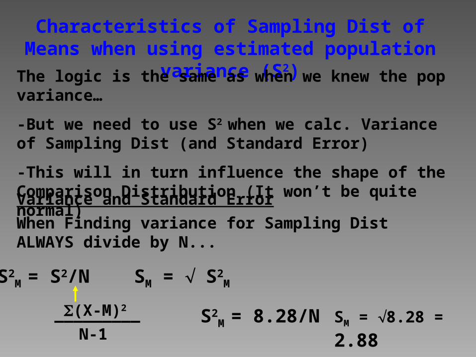
Characteristics of Sampling Dist of Means when using estimated population variance (S2)

The logic is the same as when we knew the pop variance…

-But we need to use S2 when we calc. Variance of Sampling Dist (and Standard Error)

-This will in turn influence the shape of the Comparison Distribution (It won’t be quite normal)

Variance and Standard Error

_________(X-M)2

N-1S2

M = 8.28/N SM = 8.28 = 2.88

When Finding variance for Sampling Dist ALWAYS divide by N...

S2M

= S2/N SM = S2M

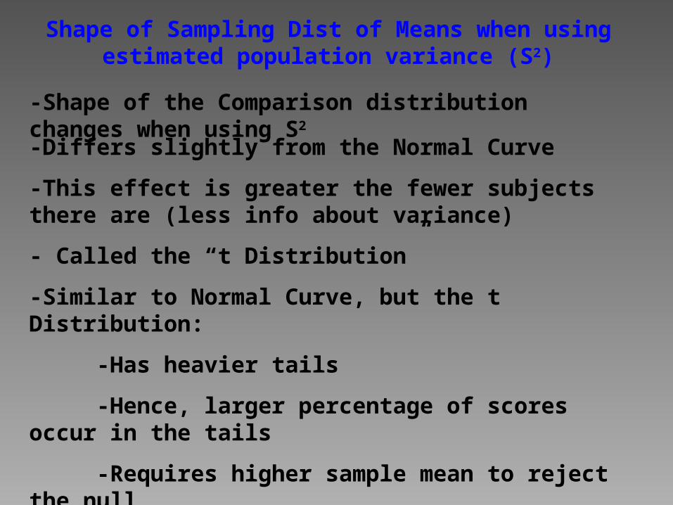
Shape of Sampling Dist of Means when using estimated population variance (S2)

-Shape of the Comparison distribution changes when using S2

-Differs slightly from the Normal Curve

-This effect is greater the fewer subjects there are (less info about variance)

- Called the “t Distribution”

-Similar to Normal Curve, but the t Distribution:

-Has heavier tails

-Hence, larger percentage of scores occur in the tails

-Requires higher sample mean to reject the null

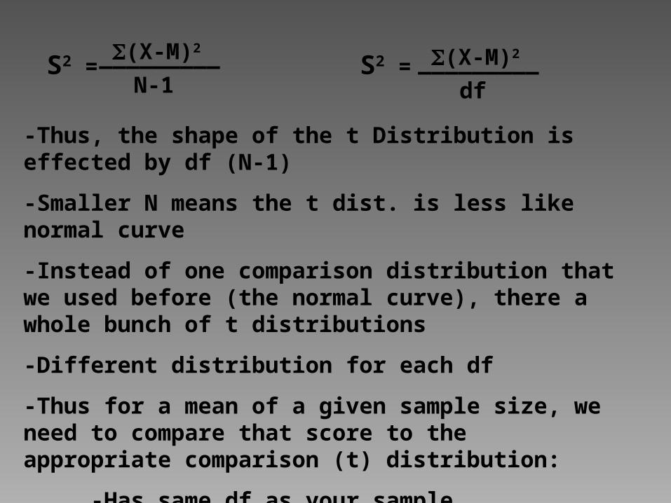
_________(X-M)2

N-1S2 = S2 = _________(X-M)2

df

-Thus, the shape of the t Distribution is effected by df (N-1)

-Smaller N means the t dist. is less like normal curve

-Instead of one comparison distribution that we used before (the normal curve), there a whole bunch of t distributions

-Different distribution for each df

-Thus for a mean of a given sample size, we need to compare that score to the appropriate comparison (t) distribution:

-Has same df as your sample

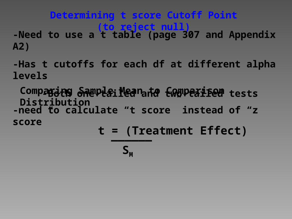
Determining t score Cutoff Point (to reject null)

-Need to use a t table (page 307 and Appendix A2)

-Has t cutoffs for each df at different alpha levels

-Both one-tailed and two-tailed tests

Comparing Sample Mean to Comparison Distribution

-need to calculate “t score” instead of “z score”

t = (Treatment Effect)

SM

______

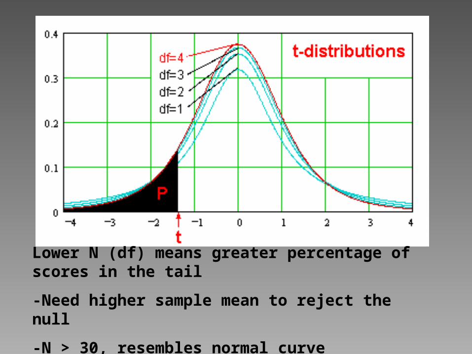
Lower N (df) means greater percentage of scores in the tail

-Need higher sample mean to reject the null

-N > 30, resembles normal curve

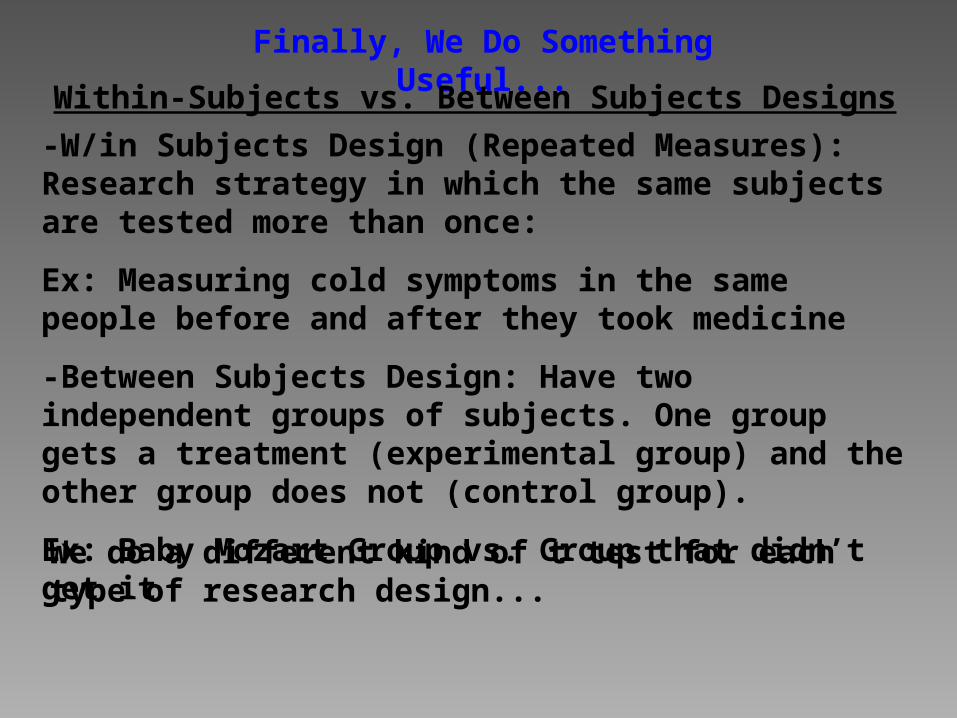
Finally, We Do Something Useful...

Within-Subjects vs. Between Subjects Designs

-W/in Subjects Design (Repeated Measures): Research strategy in which the same subjects are tested more than once:

Ex: Measuring cold symptoms in the same people before and after they took medicine

-Between Subjects Design: Have two independent groups of subjects. One group gets a treatment (experimental group) and the other group does not (control group).

Ex: Baby Mozart Group vs. Group that didn’t get it

We do a different kind of t test for each type of research design...

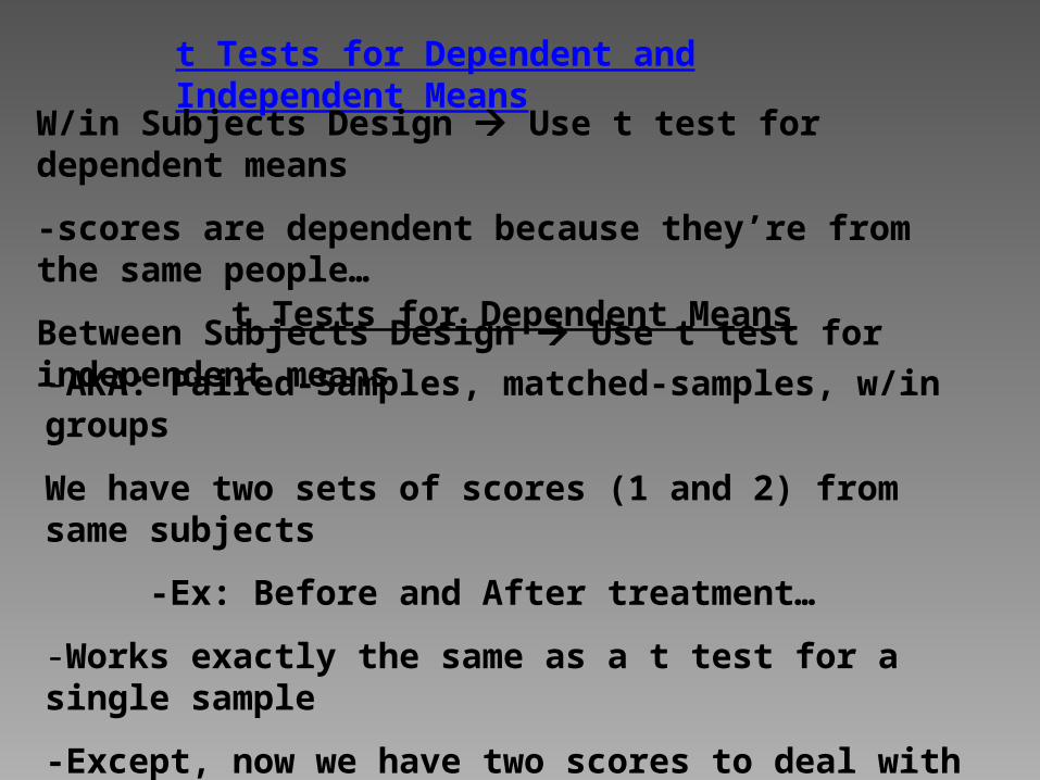
t Tests for Dependent and Independent Means

W/in Subjects Design Use t test for dependent means

-scores are dependent because they’re from the same people…

Between Subjects Design Use t test for independent means

t Tests for Dependent Means

-AKA: Paired-Samples, matched-samples, w/in groups

We have two sets of scores (1 and 2) from same subjects

-Ex: Before and After treatment…

-Works exactly the same as a t test for a single sample

-Except, now we have two scores to deal with instead of just one...

Variations of the Basic Formula for Specific t-test Varieties

W/in Subjects

t = (Treatment Effect)

SM

______

Treatment Effect equals change scores (Time 2 – Time 1)

If null hyp. is true, mean of change scores = 0

Sm of change scores used

Between Subjects

Treatment Effect equals mean of experimental group – mean of control group.

Sm is derived from a weighted estimate (based on N) of the two groups…

In other words we are controlling for proportion of the TOTAL Df contribute by each sample…

dftotal = df sample 1 + df sample 2

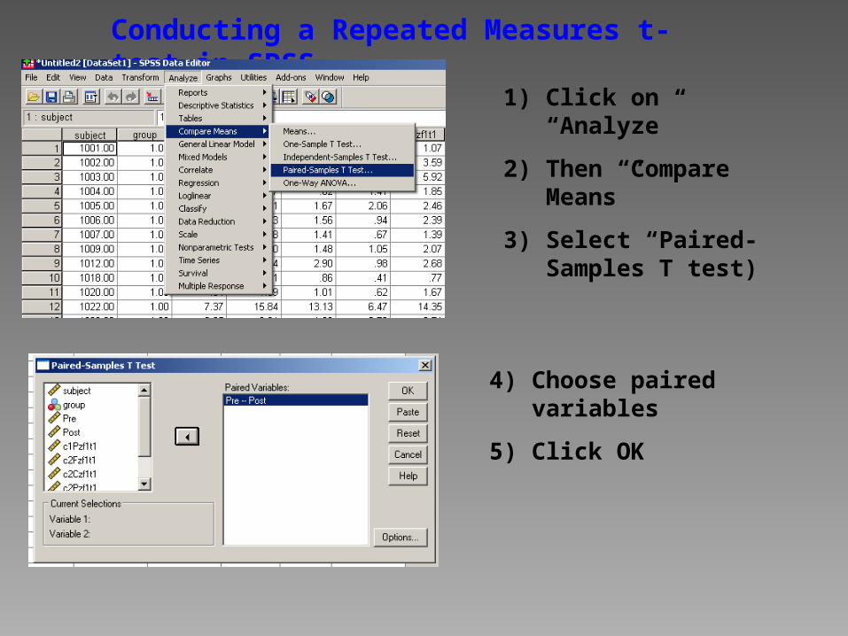
Conducting a Repeated Measures t-test in SPSS

1) Click on “Analyze”

2) Then “Compare Means”

3) Select “Paired-Samples T test)

4) Choose paired variables

5) Click OK

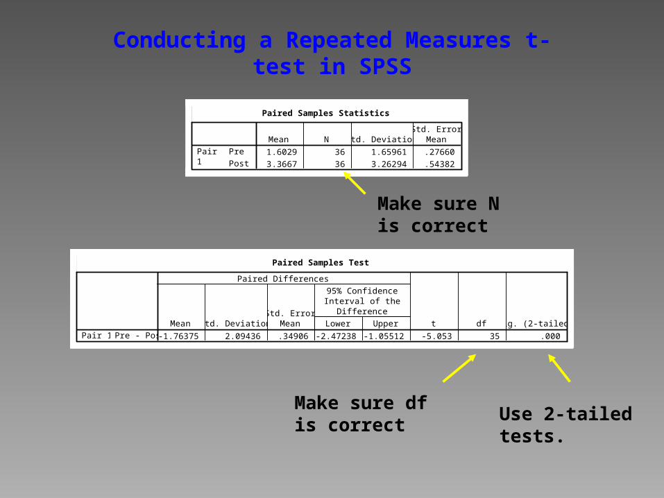
Paired Samples Test

-1.76375 2.09436 .34906 -2.47238 -1.05512 -5.053 35 .000Pre - PostPair 1Mean Std. Deviation

Std. ErrorMean Lower Upper

95% ConfidenceInterval of the

Difference

Paired Differences

t df Sig. (2-tailed)

Paired Samples Statistics

1.6029 36 1.65961 .27660

3.3667 36 3.26294 .54382

Pre

Post

Pair1

Mean N Std. DeviationStd. Error

Mean

Conducting a Repeated Measures t-test in SPSS

Make sure N is correct

Make sure df is correct

Use 2-tailed tests.

Conducting an Independent Samples t-test in SPSS

1) Click on “Analyze”

2) Then “Compare Means”

3) Select “Indpt. Samples T-test”

4) Add your D.V. here

5) Add your IV (grouping variable)

6) Click on “Define Groups”

Conducting an Independent Samples t-test in SPSS

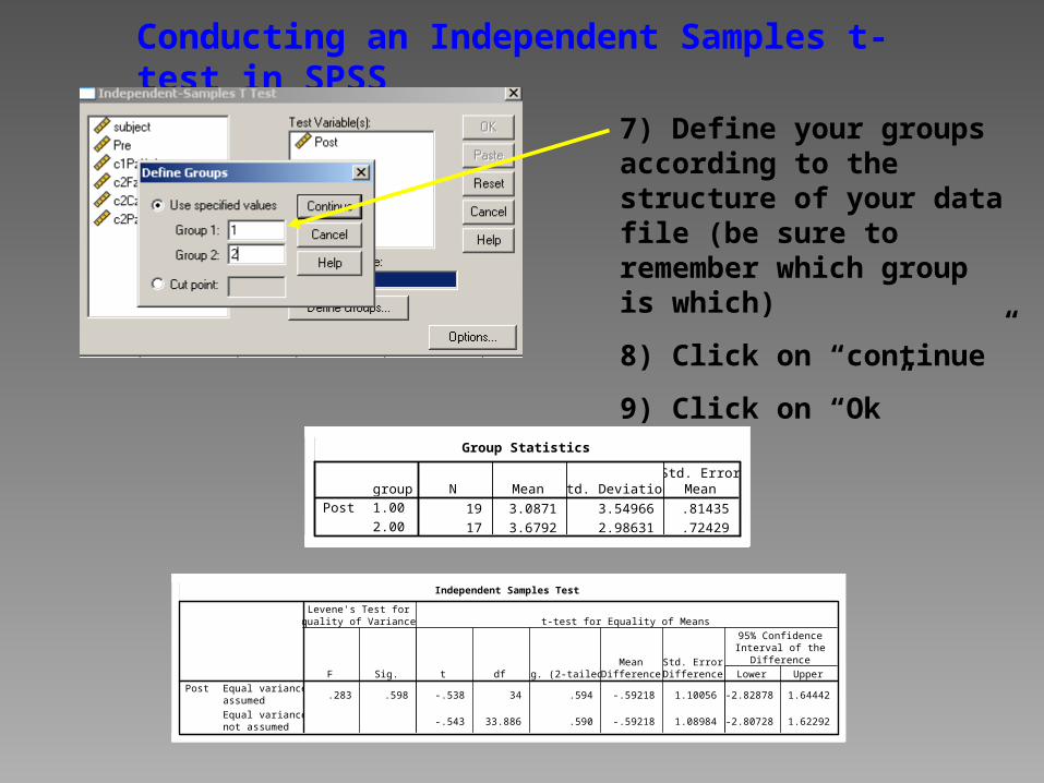
7) Define your groups according to the structure of your data file (be sure to remember which group is which)

8) Click on “continue”

9) Click on “Ok”

Independent Samples Test

.283 .598 -.538 34 .594 -.59218 1.10056 -2.82878 1.64442

-.543 33.886 .590 -.59218 1.08984 -2.80728 1.62292

Equal variancesassumed

Equal variancesnot assumed

PostF Sig.

Levene's Test forEquality of Variances

t df Sig. (2-tailed)Mean

DifferenceStd. ErrorDifference Lower Upper

95% ConfidenceInterval of the

Difference

t-test for Equality of Means

Group Statistics

19 3.0871 3.54966 .81435

17 3.6792 2.98631 .72429

group1.00

2.00

PostN Mean Std. Deviation

Std. ErrorMean

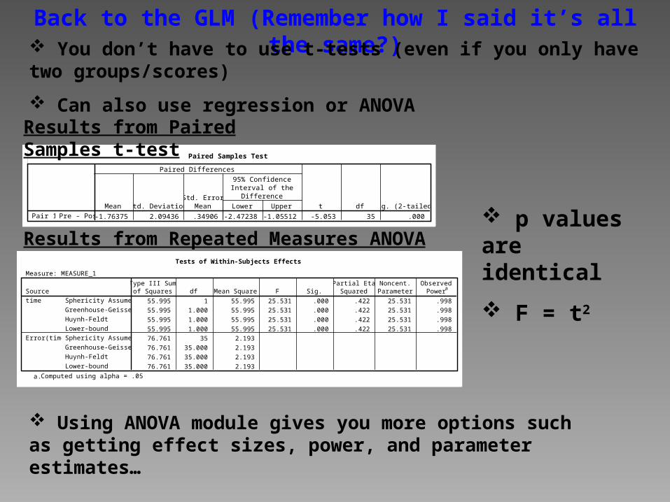
Back to the GLM (Remember how I said it’s all the same?) You don’t have to use t-tests (even if you only have two groups/scores)

Can also use regression or ANOVA

Paired Samples Test

-1.76375 2.09436 .34906 -2.47238 -1.05512 -5.053 35 .000Pre - PostPair 1Mean Std. Deviation

Std. ErrorMean Lower Upper

95% ConfidenceInterval of the

Difference

Paired Differences

t df Sig. (2-tailed)

Results from Paired Samples t-test

Tests of Within-Subjects Effects

Measure: MEASURE_1

55.995 1 55.995 25.531 .000 .422 25.531 .998

55.995 1.000 55.995 25.531 .000 .422 25.531 .998

55.995 1.000 55.995 25.531 .000 .422 25.531 .998

55.995 1.000 55.995 25.531 .000 .422 25.531 .998

76.761 35 2.193

76.761 35.000 2.193

76.761 35.000 2.193

76.761 35.000 2.193

Sphericity Assumed

Greenhouse-Geisser

Huynh-Feldt

Lower-bound

Sphericity Assumed

Greenhouse-Geisser

Huynh-Feldt

Lower-bound

Sourcetime

Error(time)

Type III Sumof Squares df Mean Square F Sig.

Partial EtaSquared

Noncent.Parameter

ObservedPower

a

Computed using alpha = .05a.

Results from Repeated Measures ANOVA p values are identical

F = t2

Using ANOVA module gives you more options such as getting effect sizes, power, and parameter estimates…

Extra Slides on Estimating Variance in Dependent Samples t-tests.

All Sorts of Estimating...

Remember, the only thing we KNOW is what we know about our samples.

-Need to use this to estimate everything else…

Estimating Population Variance

-We assume that the two populations have the same variance…

-So, we could ESTIMATE population variance from EITHER sample (or both)

-What are the chances that we would get exactly the SAME estimate of pop. variance (S2) from 2 different samples…

-So, we would get two DIFFERENT estimates for what should be the SAME #.

Estimating Population Variance

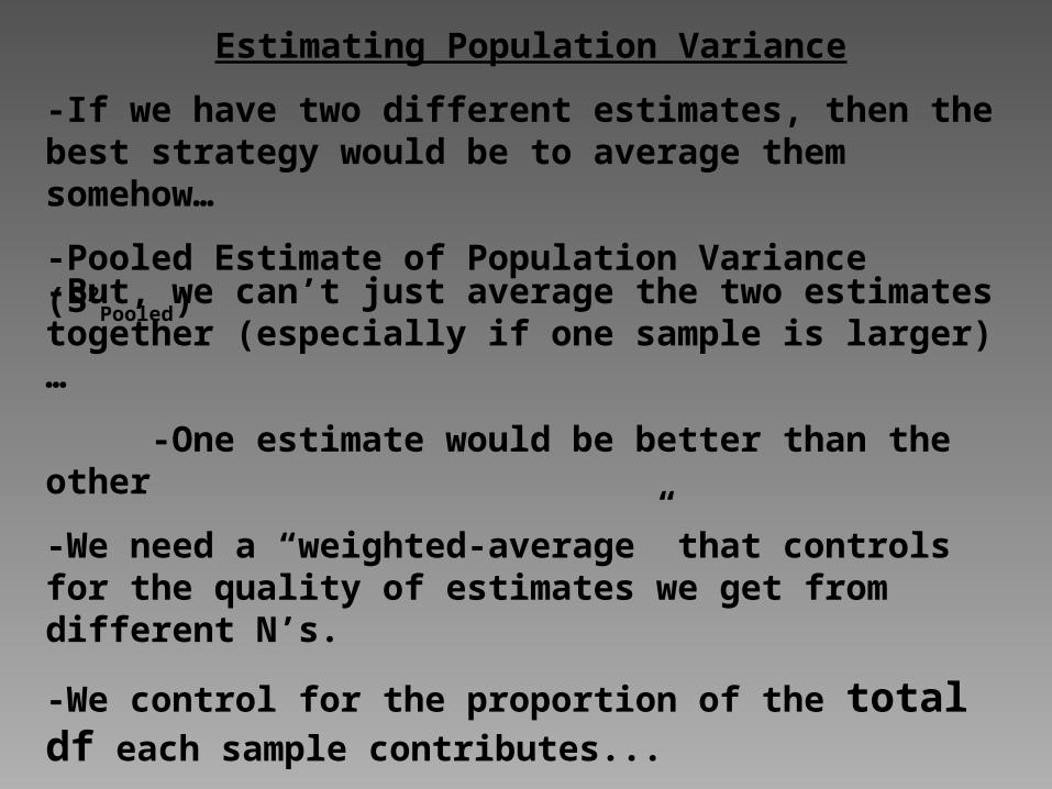
-If we have two different estimates, then the best strategy would be to average them somehow…

-Pooled Estimate of Population Variance (S2Pooled)

-But, we can’t just average the two estimates together (especially if one sample is larger)…

-One estimate would be better than the other

-We need a “weighted-average” that controls for the quality of estimates we get from different N’s.

-We control for the proportion of the total df each sample contributes...

-dftotal = df sample 1 + df sample 2

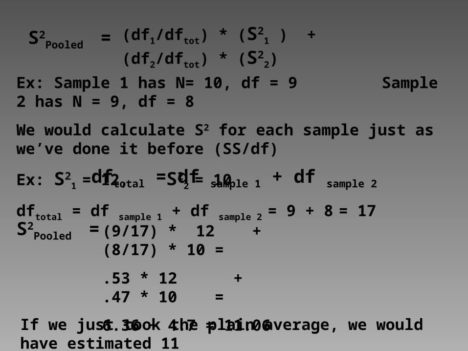
Ex: Sample 1 has N= 10, df = 9 Sample 2 has N = 9, df = 8

We would calculate S2 for each sample just as we’ve done it before (SS/df)

Ex: S21 = 12, S2

2 = 10

dftotal = df sample 1 + df sample 2 = 9 + 8 = 17

S2Pooled = (9/17) * 12 + (8/17) * 10 =

.53 * 12 + .47 * 10 =

6.36 + 4.7 = 11.06

If we just took the plain average, we would have estimated 11

S2Pooled = (df1/dftot) * (S2

1 ) + (df2/dftot) * (S22)

dftotal = df sample 1 + df sample 2

Estimating Variance of the 2 Sampling Distributions...Need to do this before we can describe the shape of the

comparison distribution (Dist. of the Differences between Means)

-We assume that the variance of the Populations of each group are the same

-But, if N is different, our estimates of the variance of the Sampling Distribution are not the same (affected by sample size)

-So we need to estimate variance of Sampling Dist. for EACH population (using the N from each sample)

S2M1 = S2

Pooled / N1 S2M2 = S2

Pooled / N2

S2M1 = 11.06/10 = 1.11 S2

M2 = 11.06/9 = 1.23

Ex:

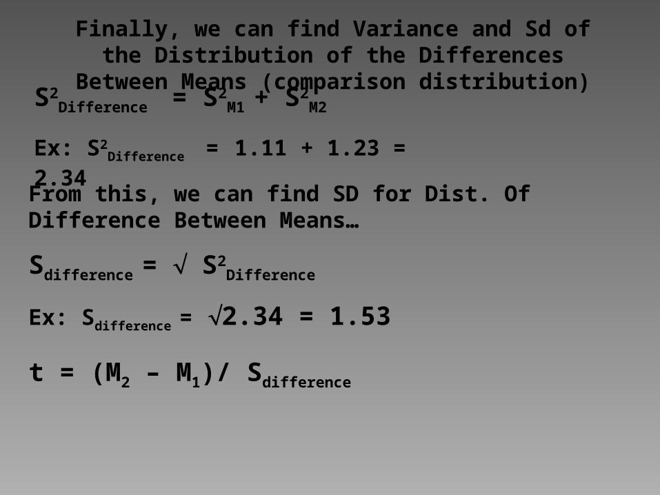
Finally, we can find Variance and Sd of the Distribution of the Differences Between Means (comparison distribution)

S2Difference = S2

M1 + S2M2

From this, we can find SD for Dist. Of Difference Between Means…

Sdifference = S2Difference

Ex: Sdifference = 2.34 = 1.53

Ex: S2Difference = 1.11 + 1.23 = 2.34

t = (M2 – M1)/ Sdifference