Embed Size (px)
Citation preview
STATS 330: Lecture 2Data Cleaning
22.07.2015

Housekeeping
I Contact details
Office email
Steffen Klaere 303.219 [email protected] Miller 303.229C [email protected]
I Course material on course website
http://www.stat.auckland.ac.nz/~stats330/
I Office hours
Steffen Klaere 9:30–10:30, Thu and FriArden Miller Wed 9–10, Thu 12-1
I Class Rep! 330 AND 762

Today’s agenda
I Data Cleaning
I Exploratory analysis

Why data cleaning?
I Analysing raw data may give misleading answers.
I Cleaning data helps to know them better.
I Anecdotally: About 80% of time for statistical analysis is datacleaning.

Steps of statistical analysis
ͳ �������������������� �� ���� �� � ������� �� ����������ǡ ��������ǡ ������������ǡ ��������������� ���� ��� ���� �� ������������ ������ �����������ǡ ���������� �����������ǡ ������������� �������� ������Ǥ
���������ǡ ���
���� ����������� ������ ������� �� ���� ��������ǡ ���������� ��� ����������� ��������� ����� �� ��������� ������� ���� ���� ��� �� ��� ������� ����� ��� ���� ��������Ǥ �� ��������ǡ � ���� ����������������� �� ������� �� ��� ���� �� ��������� ��� ���� ������ ����� ��� ����������� ���������Ǥ�� �� ���� ���� ���� ��� ��� ���� ��� ����� ���� ��� �� ��� ������� ������ǡ ��� ������� ������ǡ ����������� ��� ���� ��� ��� ������� ������ ��� ����� ���� ��� ������ ��� ��������Ǥ ���� �������� ����� ������� �� ������������ ��� ���� ���� ���������� ���� ���� ��� �� ��������Ǥ �� �� ����� ����������� ��� ������� �� ����������� ���������� ����� �� ��� ���� �� ���� �� ����� �����������Ǥ
���� �������� ��� ���������� ��ƪ����� ��� ����������� ���������� ����� �� ��� ����Ǥ �������������� ���� ���������� �� ������� �������� ��������� ��ƪ����� ��� ������� �� � �������������������Ǥ �� ���� ������ǡ ���� �������� ������ �� ���������� � ����������� ���������ǡ �� ����������� �� � ������������ ������Ǥ ��� � ����������� ����������� �������� � ��������������� ��� ������������ ���� �������� ����� ��� �������� ������� ��� �� �������� ������������ ����������Ǥ
ͳǤͳ ����������� �������� �� ϐ��� �����
�� ���� �������� � ����������� �������� �� ������ �� ��� ������ �� � ������ �� ���� ���������� ���������� ���� ���� ��������� ��� ƮƮ����� �� ��� ����ȗǤ
ǤǤǤǤǤǤǤǤǤǤǤ
����� ǣ ����������� �������� ����� �����
����� ����� �� �������� �� � ������� ������������ �������Ǥ ���� ��������� �������������� �� � ������� ����� ����� ���� ��������������� ��� ���������� ������ �� ��� ������� ����� �� ��� �����Ǥ ��� Ƥ��� ����� ȋ�������Ȍ �� ��� ���� �� �� ����� ��Ǥ ��� ����Ƥ��� ��� ���� �������ǡ ������� ����� ��������� ȋ�Ǥ�Ǥ ������� ������ �� �������Ȍǡ ������������� ������ǡ ������� �� ������������������� �������� ��� �� ��Ǥ �� �����ǡ������� ���� Ƥ��� ���� �� � ����Ŝ������������� �� ������ ��ƥ���� �� ����������������� ���� ���� �� �������������Ǥ
���� ���� ������������� ��� ����� �����ǡ���� ��� �� ������ ����������� �������Ǥ���� ��ǡ �� ���� ����� ���� ��� �� ���� ������ � ����Ŝ�����ǡ ���� ������� �����ǡ �������� ������ǡ ������� ������� �������Ǥ �������ǡ
���� ���� ��� ���� ���� ��� ������ ��� �����Ǧ���� �� ��������Ǥ �� �������ǡ �� ��� ����������� �� �������� ��������ǡ �� �����Ǧ���� ��������� �� ���������� �� ������� � ������� �������ǡ�� ���� ��� ������ �� �������Ǥ ���� ��������������� ��������� ������ �� ��� ������� ������
ȗ�� ����ǡ ���� � ����� ����� �� �� �������� ���� �� ���������� ����������� �������� ������������Ǥ
�� ������������ �� ���� �������� ���� �
de Jonge and van der Loo (2013) Statistics Netherlands

Raw data

Raw data
> sleep.df <- read.table("sleep.txt",header=T,fill=T)
> head(sleep.df)
Data from which conclusions were
1 Variables below (from left to
2 species of animal
3 body weight in kg
4 brain weight in g
5 slow wave ("nondreaming") sleep (hrs/day)
6 paradoxical ("dreaming") sleep (hrs/day)

Raw data
I May not be table form.
I May contain inadmissible characters.
I May contain inconsistent separators.
I May be technically incorrect, e.g., factor gender has levels{M, m, male, 0, F, f, female, 1}.
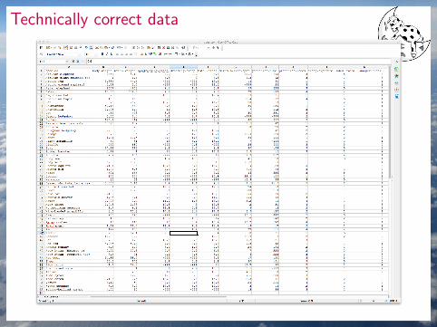
Technically correct data

Technically correct data
> sleep.df <- read.csv("sleep.csv",header=T)
> summary(sleep.df[,c(1,2,9)])
species body.weight predation.index
African elephant : 1 Min. : 0.005 Min. :1.000
African giant pouched rat: 1 1st Qu.: 0.600 1st Qu.:2.000
Arctic Fox : 1 Median : 3.342 Median :3.000
Arctic ground squirrel : 1 Mean : 198.790 Mean :2.871
Asian elephant : 1 3rd Qu.: 48.203 3rd Qu.:4.000
Baboon : 1 Max. :6654.000 Max. :5.000
(Other) :56
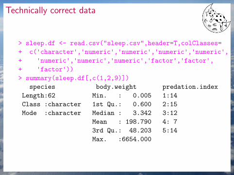
Technically correct data
> sleep.df <- read.csv("sleep.csv",header=T,colClasses=
+ c('character','numeric','numeric','numeric','numeric',+ 'numeric','numeric','numeric','factor','factor',+ 'factor'))> summary(sleep.df[,c(1,2,9)])
species body.weight predation.index
Length:62 Min. : 0.005 1:14
Class :character 1st Qu.: 0.600 2:15
Mode :character Median : 3.342 3:12
Mean : 198.790 4: 7
3rd Qu.: 48.203 5:14
Max. :6654.000

Technically correct data
I The data is stored in a data frame with suitable columnnames.
I Each column of the data frame is of adequate class.I NumericI CharacterI Factor
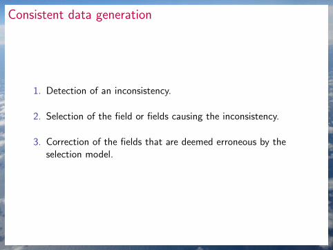
Consistent data generation
1. Detection of an inconsistency.
2. Selection of the field or fields causing the inconsistency.
3. Correction of the fields that are deemed erroneous by theselection model.

Consistent data
> summary(sleep.df[,c(4,5,6)])
nondreaming.sleep dreaming.sleep total.sleep
Min. :-999.000 Min. :-999.0 Min. :-999.00
1st Qu.: 2.375 1st Qu.: 0.5 1st Qu.: 6.20
Median : 7.400 Median : 1.3 Median : 10.30
Mean :-218.866 Mean :-194.9 Mean : -54.60
3rd Qu.: 10.550 3rd Qu.: 2.3 3rd Qu.: 13.15
Max. : 17.900 Max. : 6.6 Max. : 19.90
NA's :1
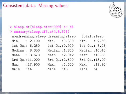
Consistent data: Missing values
> sleep.df[sleep.df==-999] <- NA
> summary(sleep.df[,c(4,5,6)])
nondreaming.sleep dreaming.sleep total.sleep
Min. : 2.100 Min. :0.300 Min. : 2.60
1st Qu.: 6.250 1st Qu.:0.900 1st Qu.: 8.05
Median : 8.350 Median :1.800 Median :10.45
Mean : 8.673 Mean :2.012 Mean :10.53
3rd Qu.:11.000 3rd Qu.:2.600 3rd Qu.:13.20
Max. :17.900 Max. :6.600 Max. :19.90
NA's :14 NA's :13 NA's :4

Consistent data: Inconsistencies
> attach(sleep.df)
> round(total.sleep-nondreaming.sleep-dreaming.sleep,1)
[1] NA 0 NA NA 0 0 0 0 0 0 0 0 0 NA 0 NA 0 0 0 0 NA 0
[23] 0 NA 0 NA 0 0 0 NA NA 0 0 0 0 0 0 0 0 0 NA 0 0 0
[45] 0 0 NA 0 0 0 0 0 NA 0 NA 0 0 0 0 0 0 NA
> detach(sleep.df)
> sleep.df[is.na(sleep.df)] <- 0
> attach(sleep.df)
> round(total.sleep-nondreaming.sleep-dreaming.sleep,1)
[1] 3.3 0.0 12.5 16.5 0.0 0.0 0.0 0.0 0.0 0.0 0.0 0.0 0.0
[14] 3.1 0.0 0.0 0.0 0.0 0.0 0.0 -0.3 0.0 0.0 12.0 0.0 13.0
[27] 0.0 0.0 0.0 10.8 0.0 0.0 0.0 0.0 0.0 0.0 0.0 0.0 0.0
[40] 0.0 -1.0 0.0 0.0 0.0 0.0 0.0 12.5 0.0 0.0 0.0 0.0 0.0
[53] 2.6 0.0 11.0 0.0 0.0 0.0 0.0 0.0 0.0 0.0
> detach(sleep.df)

Consistent data
Your data are consistent if you have dealt with
I missing values,
I special values,
I unusual observations,
I or obvious errors
in a manner suitable.

Error detection in R
> library(editrules)
> sleep.df <- within(sleep.df,{sum.sleep <-
+ round(nondreaming.sleep+dreaming.sleep,1)})> rules <- editset("total.sleep==sum.sleep")
> summary(violatedEdits(rules,sleep.df))
Edit violations, 62 observations, 0 completely missing (0%):
editname freq rel
num1 12 19.4%
Edit violations per record:
errors freq rel
0 50 80.6%
1 12 19.4%

Imputation
Missing or inconsistent data can be treated in either of thefollowing ways:
I Remove from data (seldom a good choice)I Impute reasonable alternative values by
I using the mean of the variable with missing values.I using a model to predict missing values.I randomly assign values from the range of available values.I determine value from k nearest neighbours.

Mean imputation
> summary(sleep.df$dreaming.sleep)
Min. 1st Qu. Median Mean 3rd Qu. Max. NA's0.300 0.900 1.800 2.012 2.600 6.600 13
> I <- is.na(sleep.df$dreaming.sleep)
> sleep.df$dreaming.sleep[I] <- mean(sleep.df$dreaming.sleep,na.rm=T)
> summary(sleep.df$dreaming.sleep)
Min. 1st Qu. Median Mean 3rd Qu. Max.
0.300 1.200 2.006 2.012 2.275 6.600
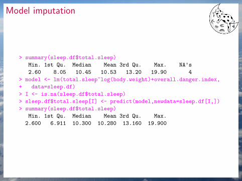
Model imputation
> summary(sleep.df$total.sleep)
Min. 1st Qu. Median Mean 3rd Qu. Max. NA's2.60 8.05 10.45 10.53 13.20 19.90 4
> model <- lm(total.sleep~log(body.weight)+overall.danger.index,
+ data=sleep.df)
> I <- is.na(sleep.df$total.sleep)
> sleep.df$total.sleep[I] <- predict(model,newdata=sleep.df[I,])
> summary(sleep.df$total.sleep)
Min. 1st Qu. Median Mean 3rd Qu. Max.
2.600 6.911 10.300 10.280 13.160 19.900

Model imputation
Body weight (log)
Tota
l sle
ep
5
10
15
20
−5 0 5
1 2
−5 0 5
3
4
−5 0 5
5
10
15
20
5

Summary data cleaning
I Create an appropriate data form (table, database).
I Check for inconsistencies.
I Deal with inconsistencies.

Thank you!