Embed Size (px)
Citation preview
Masterbook of Business and Industry (MBI)
Muhammad Firman (University of Indonesia - Accounting ‘12 ) 108
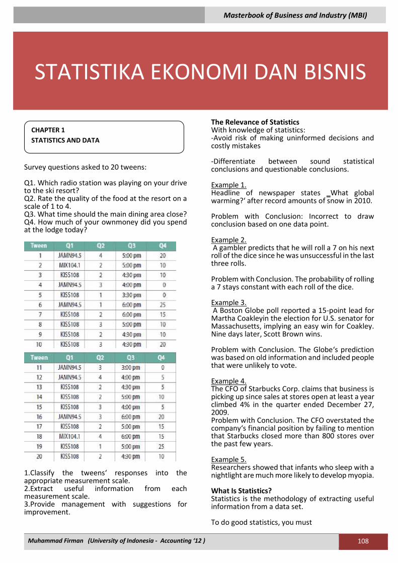
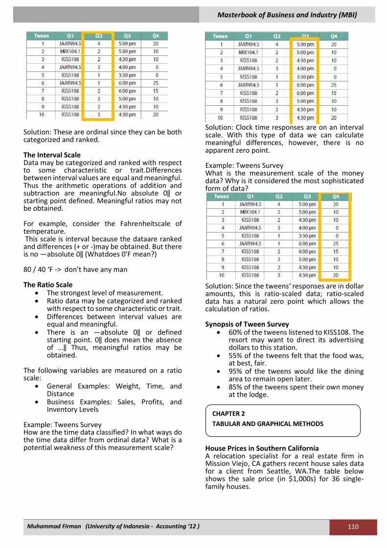
Survey questions asked to 20 tweens: Q1. Which radio station was playing on your drive to the ski resort? Q2. Rate the quality of the food at the resort on a scale of 1 to 4. Q3. What time should the main dining area close? Q4. How much of your ownmoney did you spend at the lodge today?
1.Classify the tweens‘ responses into the appropriate measurement scale. 2.Extract useful information from each measurement scale. 3.Provide management with suggestions for improvement.
The Relevance of Statistics With knowledge of statistics: -Avoid risk of making uninformed decisions and costly mistakes -Differentiate between sound statistical conclusions and questionable conclusions. Example 1. Headline of newspaper states ‗What global warming?‘ after record amounts of snow in 2010. Problem with Conclusion: Incorrect to draw conclusion based on one data point. Example 2. A gambler predicts that he will roll a 7 on his next roll of the dice since he was unsuccessful in the last three rolls. Problem with Conclusion. The probability of rolling a 7 stays constant with each roll of the dice. Example 3. A Boston Globe poll reported a 15-point lead for Martha Coakleyin the election for U.S. senator for Massachusetts, implying an easy win for Coakley. Nine days later, Scott Brown wins. Problem with Conclusion. The Globe‘s prediction was based on old information and included people that were unlikely to vote. Example 4. The CFO of Starbucks Corp. claims that business is picking up since sales at stores open at least a year climbed 4% in the quarter ended December 27, 2009. Problem with Conclusion. The CFO overstated the company‘s financial position by failing to mention that Starbucks closed more than 800 stores over the past few years. Example 5. Researchers showed that infants who sleep with a nightlight are much more likely to develop myopia. What Is Statistics? Statistics is the methodology of extracting useful information from a data set. To do good statistics, you must
CHAPTER 1
STATISTICS AND DATA
STATISTIKA EKONOMI DAN BISNIS
Masterbook of Business and Industry (MBI)
Muhammad Firman (University of Indonesia - Accounting ‘12 ) 109
1. Find the right data. 2. Use the appropriate statistical tools. 3. Clearly communicate the numerical
information into written language. Two branches of statistics
1. Descriptive Statistics : collecting, organizing, and presenting the data.
2. Inferential Statistics : drawing conclusions about a population based on sample data from that population.
Population : Consists of all items of interest. Sample : A subset of the population. A sample statistic is calculated from the sample data and is used to make inferences about the population parameter. Reasons for sampling from the population
1. Too expensive to gather information on the entire population
2. Often impossible to gather information on the entire population
Cross-sectional data
• Data collected by recording a characteristic of many subjects at the same point in time, or without regard to differences in time.
• Subjects might include individuals, households, firms, industries, regions, and countries.
• The survey data from the Introductory Case is an example of cross-sectional data.
Types of Data Time series data Data collected by recording a characteristic of a subject over several time periods.Data can include daily, weekly, monthly, quarterly, or annual observations.This graph plots the U.S. GDP growth rate from 1980 to 2010 -it is an example of time series data. Variables and Scales of Measurement A variable is the general characteristic being observed on an object of interest. Types of Variables
1. Qualitative –gender, race, political affiliation
2. Quantitative –test scores, age, weight Discrete Continuous
Types of Quantitative Variables Discrete A discrete variable assumes a countable number of distinct values.Examples: Number of children in
a family, number of points scored in a basketball game. Continuous A continuous variable can assume an infinite number of values within some interval.Examples: Weight, height, investment return. Scales of Measure
The Nominal Scale
• The least sophisticated level of measurement.
• Data are simply categories for grouping the data.
• Qualitative values may be converted to quantitative values for analysis purposes.
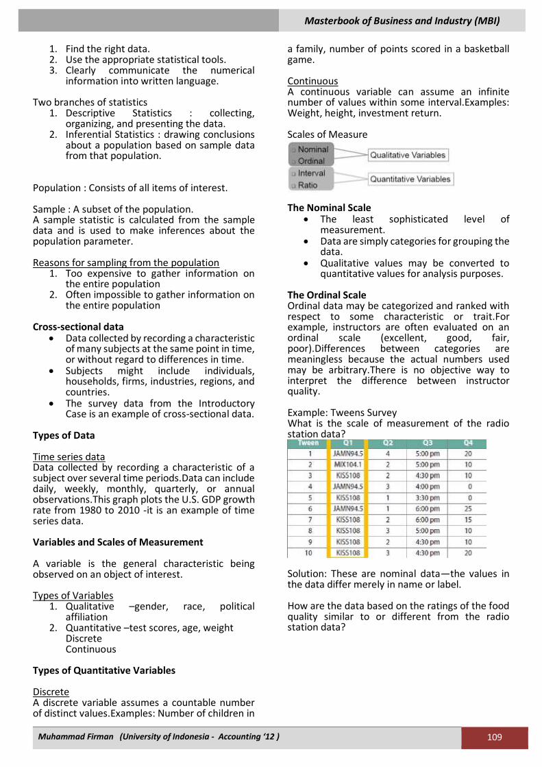
The Ordinal Scale Ordinal data may be categorized and ranked with respect to some characteristic or trait.For example, instructors are often evaluated on an ordinal scale (excellent, good, fair, poor).Differences between categories are meaningless because the actual numbers used may be arbitrary.There is no objective way to interpret the difference between instructor quality. Example: Tweens Survey What is the scale of measurement of the radio station data?
Solution: These are nominal data—the values in the data differ merely in name or label. How are the data based on the ratings of the food quality similar to or different from the radio station data?
Masterbook of Business and Industry (MBI)
Muhammad Firman (University of Indonesia - Accounting ‘12 ) 110
Solution: These are ordinal since they can be both categorized and ranked. The Interval Scale Data may be categorized and ranked with respect to some characteristic or trait.Differences between interval values are equal and meaningful. Thus the arithmetic operations of addition and subtraction are meaningful.No absolute 0‖ or starting point defined. Meaningful ratios may not be obtained. For example, consider the Fahrenheitscale of temperature. This scale is interval because the dataare ranked and differences (+ or -)may be obtained. But there is no ―absolute 0‖ (Whatdoes 0’F mean?) 80 / 40 ‘F -> don’t have any man The Ratio Scale
• The strongest level of measurement. • Ratio data may be categorized and ranked
with respect to some characteristic or trait. • Differences between interval values are
equal and meaningful. • There is an ―absolute 0‖ or defined
starting point. 0‖ does mean the absence of …‖ Thus, meaningful ratios may be obtained.
The following variables are measured on a ratio scale:
• General Examples: Weight, Time, and Distance
• Business Examples: Sales, Profits, and Inventory Levels
Example: Tweens Survey How are the time data classified? In what ways do the time data differ from ordinal data? What is a potential weakness of this measurement scale?
Solution: Clock time responses are on an interval scale. With this type of data we can calculate meaningful differences, however, there is no apparent zero point. Example: Tweens Survey What is the measurement scale of the money data? Why is it considered the most sophisticated form of data?
Solution: Since the tweens‘ responses are in dollar amounts, this is ratio-scaled data; ratio-scaled data has a natural zero point which allows the calculation of ratios. Synopsis of Tween Survey
• 60% of the tweens listened to KISS108. The resort may want to direct its advertising dollars to this station.
• 55% of the tweens felt that the food was, at best, fair.
• 95% of the tweens would like the dining area to remain open later.
• 85% of the tweens spent their own money at the lodge.
House Prices in Southern California A relocation specialist for a real estate firm in Mission Viejo, CA gathers recent house sales data for a client from Seattle, WA.The table below shows the sale price (in $1,000s) for 36 single-family houses.
CHAPTER 2
TABULAR AND GRAPHICAL METHODS
Masterbook of Business and Industry (MBI)
Muhammad Firman (University of Indonesia - Accounting ‘12 ) 111
Use the sample information to: 1. Summarize the range of house prices. 2. Comment on where house prices tend to cluster. 3. Calculate percentages to compare house prices. Summarizing Qualitative Data A frequency distribution for qualitative data groups data into categories and records how many observations fall into each category.Weather conditions in Seattle, WA during February 2010.
• Categories: Rainy, Sunny, or Cloudy. • For each category‘s frequency, count the
days that fall in that category. • Calculate relative frequencyby dividing
each category‘s frequency by the sample size !
To express relative frequencies in terms of percentages, multiply each proportion by 100%. Note that the total of the proportions must add to 1.0 and the total of the percentages must add to 100%.
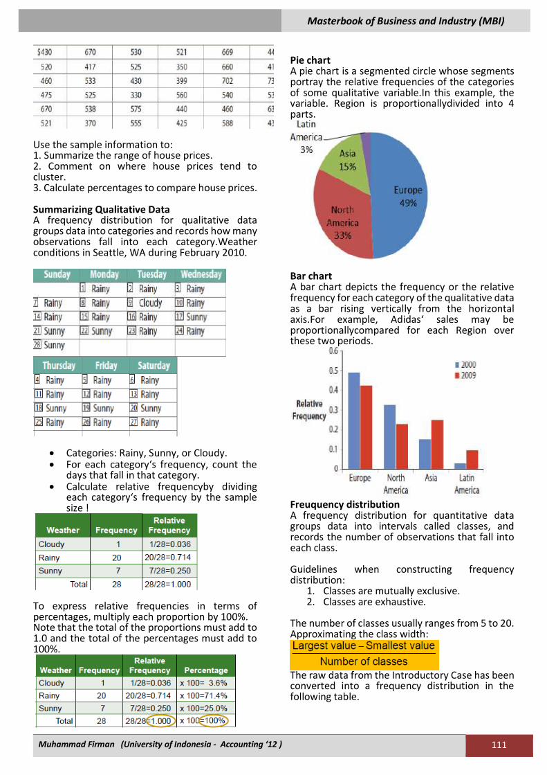
Pie chart A pie chart is a segmented circle whose segments portray the relative frequencies of the categories of some qualitative variable.In this example, the variable. Region is proportionallydivided into 4 parts.
Bar chart A bar chart depicts the frequency or the relative frequency for each category of the qualitative data as a bar rising vertically from the horizontal axis.For example, Adidas‘ sales may be proportionallycompared for each Region over these two periods.
Freuquency distribution A frequency distribution for quantitative data groups data into intervals called classes, and records the number of observations that fall into each class. Guidelines when constructing frequency distribution:
1. Classes are mutually exclusive. 2. Classes are exhaustive.
The number of classes usually ranges from 5 to 20. Approximating the class width:
The raw data from the Introductory Case has been converted into a frequency distribution in the following table.
Masterbook of Business and Industry (MBI)
Muhammad Firman (University of Indonesia - Accounting ‘12 ) 112
Question: What is the price range over this time period? Answer : $300,000 up to $800,000 Question: How many of the houses sold in the $500,000 up to $600,000 range? Answer : 14 houses Cumulative frequency distribution A cumulative frequency distribution specifies how many observations fall below the upper limit of a particular class.
Question: How many of the houses sold for less than $600,000? Answers : 29 houses Relative Frequency distribution A relative frequency distribution identifies theproportion or fraction of values that fall into eachclass.
Cumulative Frequency distribution A cumulative relative frequency distributiongives the proportion or fraction of values that fallbelow the upper limit of each class. Here are the relative frequency and the cumulative relative frequency distributions for the house-price data.
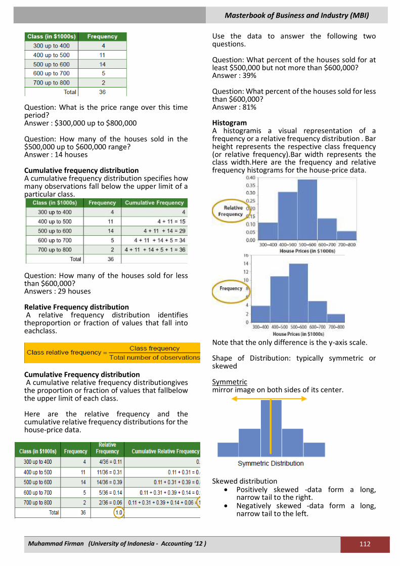
Use the data to answer the following two questions. Question: What percent of the houses sold for at least $500,000 but not more than $600,000? Answer : 39% Question: What percent of the houses sold for less than $600,000? Answer : 81% Histogram A histogramis a visual representation of a frequency or a relative frequency distribution . Bar height represents the respective class frequency (or relative frequency).Bar width represents the class width.Here are the frequency and relative frequency histograms for the house-price data.
Note that the only difference is the y-axis scale. Shape of Distribution: typically symmetric or skewed Symmetric mirror image on both sides of its center.
Skewed distribution
• Positively skewed -data form a long, narrow tail to the right.
• Negatively skewed -data form a long, narrow tail to the left.
Masterbook of Business and Industry (MBI)
Muhammad Firman (University of Indonesia - Accounting ‘12 ) 113
Polygon A polygonis a visual representation of a frequency or a relative frequency distribution.Plot the class midpoints on x-axis and associated frequency (or relative frequency) on y-axis.Neighboring points are connected with a straight line. Here is a polygon for the house-price data.
Ogive An ogiveis a visual representation of a cumulative frequency or a cumulative relative frequency distribution.Plot the cumulative frequency (or cumulative relative frequency) of each class above the upper limit of the corresponding class.The neighboring points are then connected. Here is an ogive for the house-price data.
Question : Use the ogive to approximate the percentage of houses that sold for less than $550,000. Answer: 60% Stem-and-Leaf Diagrams A stem-and-leaf diagram provides a visual display of quantitative data.
• It gives an overall picture of the data‘s center and variability.
• Each value of the data set is separated into two parts: the stemconsists of the leftmost digits, while the leafis the last digit.
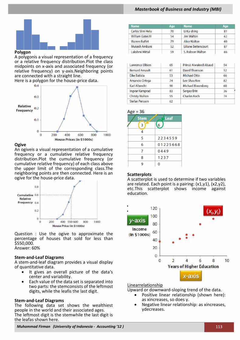
Stem-and-Leaf Diagrams The following data set shows the wealthiest people in the world and their associated ages. The leftmost digit is the stemwhile the last digit is the leafas shown here.
Age = 36
Scatterplots A scatterplot is used to determine if two variables are related. Each point is a pairing: (x1,y1), (x2,y2), etc.This scatterplot shows income against education.
Linearrelationship Upward or downward-sloping trend of the data.
• Positive linear relationship (shown here): as xincreases, so does y.
• Negative linear relationship: as xincreases, ydecreases.
Masterbook of Business and Industry (MBI)
Muhammad Firman (University of Indonesia - Accounting ‘12 ) 114
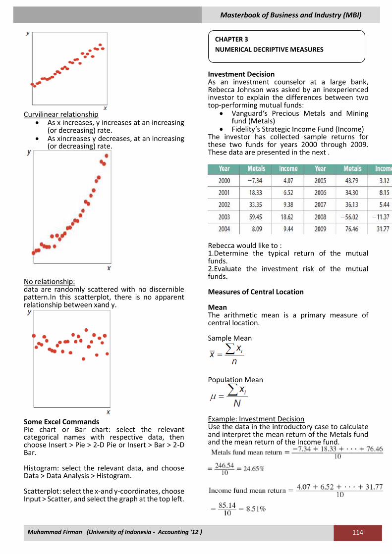
Curvilinear relationship
• As x increases, y increases at an increasing (or decreasing) rate.
• As xincreases y decreases, at an increasing (or decreasing) rate.
No relationship: data are randomly scattered with no discernible pattern.In this scatterplot, there is no apparent relationship between xand y.
Some Excel Commands Pie chart or Bar chart: select the relevant categorical names with respective data, then choose Insert > Pie > 2-D Pie or Insert > Bar > 2-D Bar. Histogram: select the relevant data, and choose Data > Data Analysis > Histogram. Scatterplot: select the x-and y-coordinates, choose Input > Scatter, and select the graph at the top left.
Investment Decision As an investment counselor at a large bank, Rebecca Johnson was asked by an inexperienced investor to explain the differences between two top-performing mutual funds:
• Vanguard‘s Precious Metals and Mining fund (Metals)
• Fidelity‘s Strategic Income Fund (Income) The investor has collected sample returns for these two funds for years 2000 through 2009. These data are presented in the next .
Rebecca would like to : 1.Determine the typical return of the mutual funds. 2.Evaluate the investment risk of the mutual funds. Measures of Central Location Mean The arithmetic mean is a primary measure of central location. Sample Mean
Population Mean
Example: Investment Decision Use the data in the introductory case to calculate and interpret the mean return of the Metals fund and the mean return of the Income fund.
CHAPTER 3
NUMERICAL DECRIPTIVE MEASURES
Masterbook of Business and Industry (MBI)
Muhammad Firman (University of Indonesia - Accounting ‘12 ) 115
The mean is sensitive to outliers. Consider the salaries of employees at Acetech.
This mean does not reflect the typical salary! Median The medianis another measure of central location that is not affected by outliers.When the data are arranged in ascending order, the median isthe middle value if the number of observations is odd, orthe average of the two middle values if the number of observations is even. Consider the sorted salaries of employees at Acetech (odd number).
Median = 90,000 Consider the sorted data from the Metals funds of the introductory case study (even number).
Median = (33.35 + 34.30) / 2 = 33.83%. Mode The modeis another measure of central location.
• The most frequently occurring value in a data set
• Used to summarize qualitative data • A data set can have no mode, one mode
(unimodal), or many modes (multimodal). Consider the salary of employees at Acetech
The mode is $40,000 since this value appears most often. Percentiles and Box Plots
In general, the pth percentiledivides a data set into two parts:
• Approximately p percent of the observations have values less than the pth percentile;
• Approximately (100 - p) percent of the observations have values greater than the pth percentile.LO 3.2 Calculate and interpret percentiles and a box plot.
Calculating the pth percentile:
• First arrange the data in ascending order. • Locate the position, Lp, of the pth
percentile by using the formula:
We use this position to find the percentile as shown next. Consider the sorted data from the introductory case.
For the 25th percentile, we locate the position:
Similarly, for the 75th percentile, we first find:
Calculating the pth percentile Once you find Lp, observe whether or not itis an integer.
• If Lpis an integer, then the Lpthobservationin the sorted data set is the pth percentile.
• If Lp is not an integer, then interpolate between two corresponding observations to approximate the pth percentile.
Both L25 = 2.75 and L75 = 8.25 are not integers, thusThe 25th percentile is located 75% of the distance between the second and third observations, and it is
The 75th percentile is located 25% of the distance between the eighth and ninth observations, and it is
Percentiles and Box Plots A box plot allows you to:
• Graphically display the distribution of a data set.
• Compare two or more distributions. • Identify outliers in a data set.
Masterbook of Business and Industry (MBI)
Muhammad Firman (University of Indonesia - Accounting ‘12 ) 116
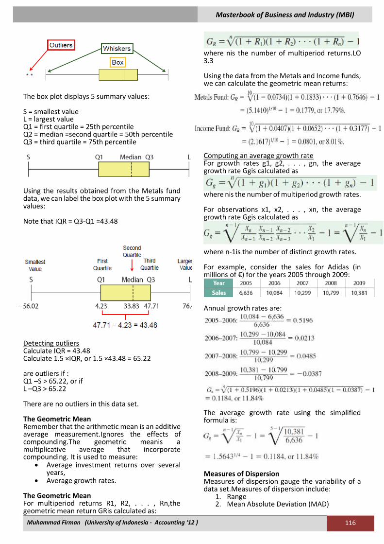
The box plot displays 5 summary values: S = smallest value L = largest value Q1 = first quartile = 25th percentile Q2 = median =second quartile = 50th percentile Q3 = third quartile = 75th percentile
Using the results obtained from the Metals fund data, we can label the box plot with the 5 summary values: Note that IQR = Q3-Q1 =43.48
Detecting outliers Calculate IQR = 43.48 Calculate 1.5 ×IQR, or 1.5 ×43.48 = 65.22 are outliers if : Q1 –S > 65.22, or if L –Q3 > 65.22 There are no outliers in this data set. The Geometric Mean Remember that the arithmetic mean is an additive average measurement.Ignores the effects of compounding.The geometric meanis a multiplicative average that incorporate compounding. It is used to measure:
• Average investment returns over several years,
• Average growth rates. The Geometric Mean For multiperiod returns R1, R2, . . . , Rn,the geometric mean return GRis calculated as:
where nis the number of multiperiod returns.LO 3.3 Using the data from the Metals and Income funds, we can calculate the geometric mean returns:
Computing an average growth rate For growth rates g1, g2, . . . , gn, the average growth rate Ggis calculated as
where nis the number of multiperiod growth rates. For observations x1, x2, . . . , xn, the average growth rate Ggis calculated as
where n-1is the number of distinct growth rates. For example, consider the sales for Adidas (in millions of €) for the years 2005 through 2009:
Annual growth rates are:
The average growth rate using the simplified formula is:
Measures of Dispersion Measures of dispersion gauge the variability of a data set.Measures of dispersion include:
1. Range 2. Mean Absolute Deviation (MAD)
Masterbook of Business and Industry (MBI)
Muhammad Firman (University of Indonesia - Accounting ‘12 ) 117
3. Variance and Standard Deviation 4. Coefficient of Variation (CV)
Measures of Dispersion Range
• It is the simplest measure. • It is focusses on extreme values.
Range = Maximum Value - Minimum Value Calculate the range using the data from the Metalsand Income funds !
Measures of Dispersion Mean Absolute Deviation (MAD) MAD is an average of the absolute difference of each observation from the mean.
Calculate MAD using the data from the Metals fund.
Varianceand standard deviation For a given sample,
For a given population,
Calculate the variance and the standard deviation using the data from the Metals fund.
Coefficient of variation (CV)
• CV adjusts for differences in the magnitudes of the means.
• CV is unitless, allowing easy comparisons of mean-adjusted dispersion across different data sets.
Calculate the coefficient of variation (CV) using the data from the Metals fund and the Income fund
Synopsis of Investment Decision
• Mean and median returns for the Metals fund are 24.65% and 33.83%, respectively.
• Mean and median returns for the Income fund are 8.51% and 7.34%, respectively.
• The standard deviation for the Metals fund and the Income fund are 37.13% and 11.07%, respectively.
• The coefficient of variation for the Metals fund and the Income fund are 1.51 and 1.30, respectively.
Mean-Variance Analysis and the Sharpe Ratio Mean-variance analysis:
• The performance of an asset is measured by its rate of return.
• The rate of return may be evaluated in terms of its reward (mean) and risk (variance).
• Higher average returns are often associated with higher risk.
The Sharpe ratio uses the mean and variance to evaluate risk. Sharpe Ratio Measures the extra reward per unit of risk. For an investment І , the Sharpe ratio is computed as:
where
Masterbook of Business and Industry (MBI)
Muhammad Firman (University of Indonesia - Accounting ‘12 ) 118
Sharpe Ratio Example Compute the Sharpe ratios for the Metals and Income funds given the risk free return of 4%.
Since 0.56 > 0.41, the Metals fund offers more reward per unit of risk as compared to the Income fund. Chebyshev’s Theorem and the Empirical Rule Chebyshev’s Theorem For any data set, the proportion of observations that lie within k standard deviations from the mean is at least 1-1/k2 , where k is any number greater than 1. Consider a large lecture class with 280 students. The mean score on an exam is 74 with a standard deviation of 8. At least how many students scored within 58 and 90? With k = 2, we have 1-1/22= 0.75. At least 75% of 280 or 210 students scored within 58 and 90. The Empirical Rule: Approximately 68% of all observations fall in the interval .
Approximately 95% of all observations fall in the interval .
Almost all observations fall in the interval.
Reconsider the example of the lecture class with 280 students with a mean score of 74 and a standard deviation of 8. Assume that the distribution is symmetric and bell-shaped. Approximately how many students scored within 58 and 90?
• The score 58 is two standard deviations below the mean while the score 90 is two standard deviations above the mean.
• Therefore about 95% of 280 students, or 0.95(280) = 266 students, scored within 58 and 90.
When data are grouped or aggregated, we use these formulas:
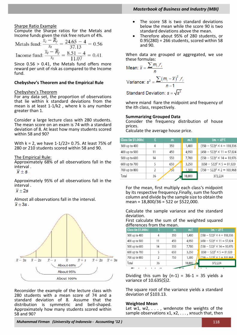
where miand fiare the midpoint and frequency of the ith class, respectively. Summarizing Grouped Data Consider the frequency distribution of house prices. Calculate the average house price.
For the mean, first multiply each class‘s midpoint by its respective frequency.Finally, sum the fourth column and divide by the sample size to obtain the mean = 18,800/36 = 522 or $522,000. Calculate the sample variance and the standard deviation. First calculate the sum of the weighted squared differences from the mean.
Dividing this sum by (n-1) = 36-1 = 35 yields a variance of 10.635($)2. The square root of the variance yields a standard deviation of $103.13. Weighted Mean Let w1, w2, . . . , wndenote the weights of the sample observations x1, x2, . . . , xnsuch that, then
Masterbook of Business and Industry (MBI)
Muhammad Firman (University of Indonesia - Accounting ‘12 ) 119
A student scores 60 on Exam 1, 70 on Exam 2, and 80 on Exam 3. What is the student‘s average score for the course if Exams 1, 2, and 3 are worth 25%, 25%, and 50% of the grade, respectively? Define w1= 0.25, w2= 0.25, and w3= 0.50.
The unweighted mean is only 70 as it does not incorporate the higher weight given to the score on Exam 3. Covariance and Correlation
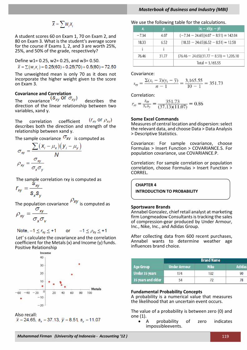
The covariance describes the direction of the linear relationship between two variables, xand y. The correlation coefficient describes both the direction and strength of the relationship between xand y.
The sample covariance is computed as
The sample correlation rxy is computed as
The population covariance is computed as
Let‘ s calculate the covariance and the correlation coefficient for the Metals (x) and Income (y) funds. Positive Relationship
Also recall:
We use the following table for the calculations.
Covariance:
Correlation:
Some Excel Commands Measures of central location and dispersion: select the relevant data, and choose Data > Data Analysis > Descriptive Statistics. Covariance: For sample covariance, choose Formulas > Insert Function > COVARIANCE.S. For population covariance, use COVARIANCE.P. Correlation: For sample correlation or population correlation, choose Formulas > Insert Function > CORREL.
Sportsware Brands Annabel Gonzalez, chief retail analyst at marketing firm Longmeadow Consultants is tracking the sales of compression-gear produced by Under Armour, Inc., Nike, Inc., and Adidas Group. After collecting data from 600 recent purchases, Annabel wants to determine weather age influences brand choice.
Fundamental Probability Concepts A probability is a numerical value that measures the likelihood that an uncertain event occurs. The value of a probability is between zero (0) and one (1).
• A probability of zero indicates impossibleevents.
CHAPTER 4
INTRODUCTION TO PROBABILITY
Masterbook of Business and Industry (MBI)
Muhammad Firman (University of Indonesia - Accounting ‘12 ) 120
• A probability of one indicates definiteevents.
An experimentis a trial that results in one of several uncertain outcomes. Example: Trying to assess the probability of a snowboarder winning a medal in the ladies‘ halfpipe event while competing in the Winter Olympic Games. Solution: The athlete‘s attempt to predict her chances of medaling is an experiment because the outcome is unknown.
• The athlete‘s competition has four possible outcomes: gold medal, silver medal, bronze medal, and no medal. We formally write the sample space as S = {gold, silver, bronze, no medal}.
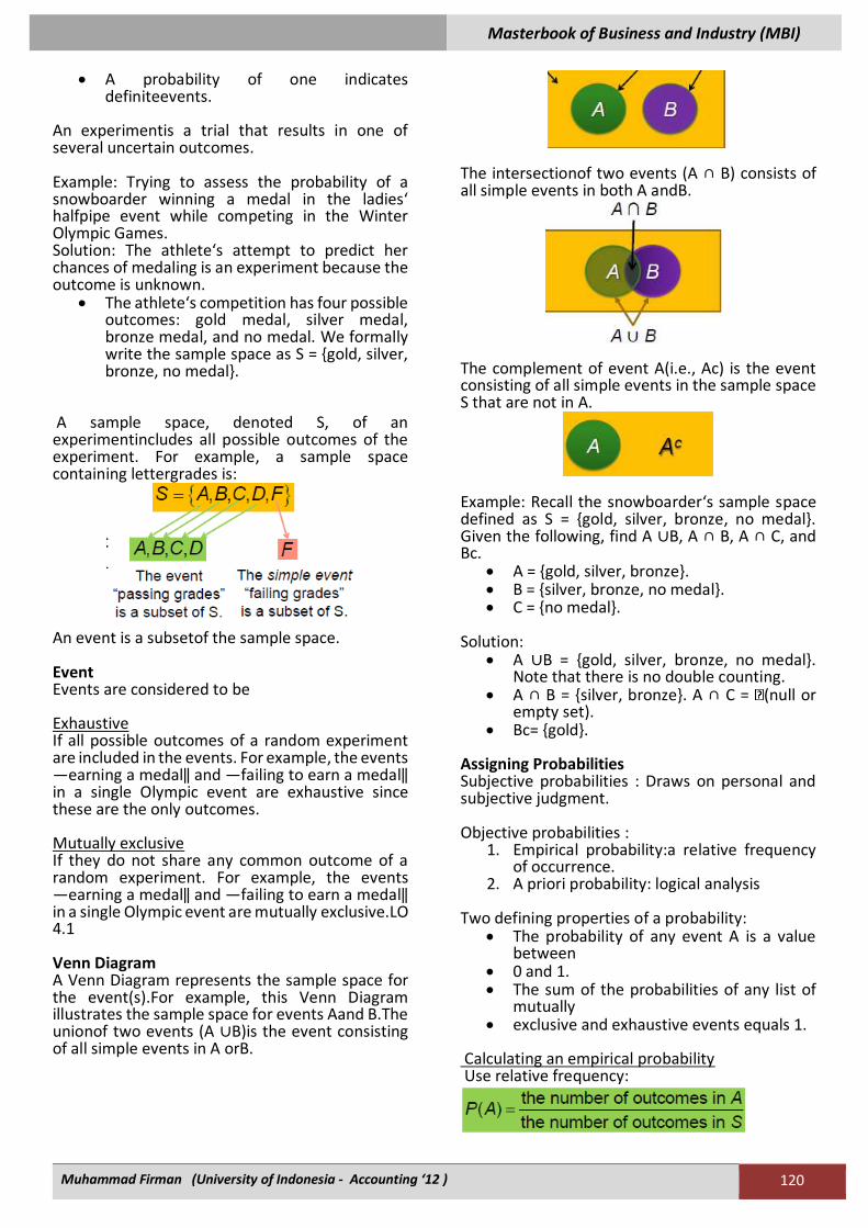
A sample space, denoted S, of an experimentincludes all possible outcomes of the experiment. For example, a sample space containing lettergrades is:
An event is a subsetof the sample space. Event Events are considered to be Exhaustive If all possible outcomes of a random experiment are included in the events. For example, the events ―earning a medal‖ and ―failing to earn a medal‖ in a single Olympic event are exhaustive since these are the only outcomes. Mutually exclusive If they do not share any common outcome of a random experiment. For example, the events ―earning a medal‖ and ―failing to earn a medal‖ in a single Olympic event are mutually exclusive.LO 4.1 Venn Diagram A Venn Diagram represents the sample space for the event(s).For example, this Venn Diagram illustrates the sample space for events Aand B.The unionof two events (A ∪B)is the event consisting of all simple events in A orB.
The intersectionof two events (A ∩ B) consists of all simple events in both A andB.
The complement of event A(i.e., Ac) is the event consisting of all simple events in the sample space S that are not in A.
Example: Recall the snowboarder‘s sample space defined as S = {gold, silver, bronze, no medal}. Given the following, find A ∪B, A ∩ B, A ∩ C, and Bc.
• A = {gold, silver, bronze}. • B = {silver, bronze, no medal}. • C = {no medal}.
Solution:
• A ∪B = {gold, silver, bronze, no medal}. Note that there is no double counting.
• A ∩ B = {silver, bronze}. A ∩ C = (null or empty set).
• Bc= {gold}. Assigning Probabilities Subjective probabilities : Draws on personal and subjective judgment. Objective probabilities :
1. Empirical probability:a relative frequency of occurrence.
2. A priori probability: logical analysis Two defining properties of a probability:
• The probability of any event A is a value between
• 0 and 1. • The sum of the probabilities of any list of
mutually • exclusive and exhaustive events equals 1.
Calculating an empirical probability Use relative frequency:
Masterbook of Business and Industry (MBI)
Muhammad Firman (University of Indonesia - Accounting ‘12 ) 121
Example: Let event A be the probability of earning a medal: P(A) = P({gold}) + P({silver}) + P({bronze}) = 0.10 + 0.15 + 0.20 = 0.45. P(B ∪C) = P({silver}) + P({bronze}) + P({no medal}) = 0.15 + 0.20 + 0.55 = 0.90. P(A ∩ C) = 0; recall that there are no common outcomes in A and C. P(Bc) = P({gold}) = 0.10. Probabilities expressed as odds. Percentagesand odds are an alternative approach to expressing probabilities include. Converting an odds ratio to a probability: Given odds forevent Aoccurring of ―a to b,‖ the probability of Ais:
Given odds againstevent Aoccurring of ―a to b,‖ the probability of Ais:
Converting a probability to an odds ratio: The odds forevent A occurring is equal to
The odds againstAn occurring is equal to
Example: Converting an odds ratio to a probability. Given the odds of 2:1 for beating the Cardinals, what was the probability of the Steelers‘ winning just prior to the 2009 Super Bowl?
Example: Converting a probabilityto an odds ratio. Given that the probability of an on-time arrival for New York‘s Kennedy Airport is 0.56, what are the odds for a plane arriving on-time at Kennedy Airport?
Rules of Probability The Complement Rule The probability of the complement of an event,P(Ac), is equal to one minus the probability of theevent.
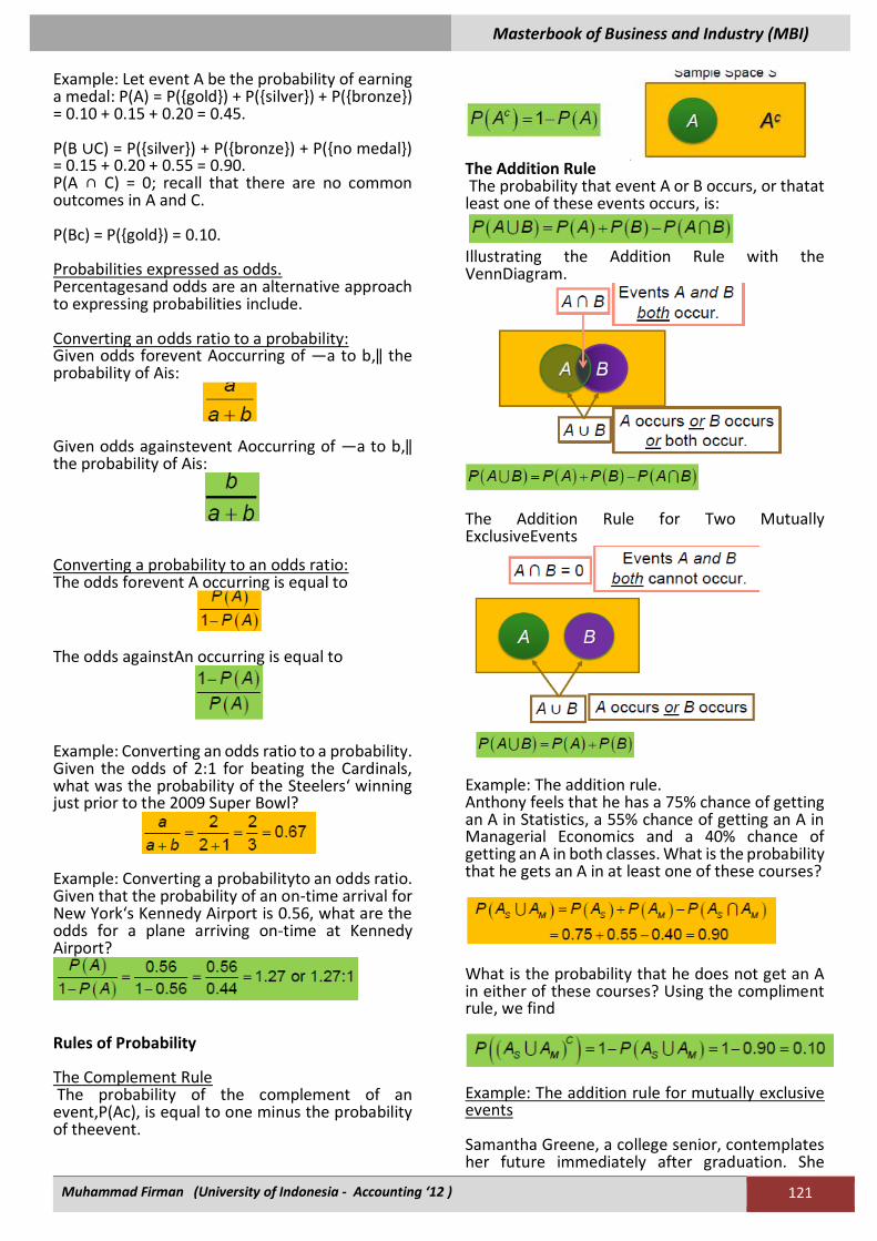
The Addition Rule The probability that event A or B occurs, or thatat least one of these events occurs, is:
Illustrating the Addition Rule with the VennDiagram.
The Addition Rule for Two Mutually ExclusiveEvents
Example: The addition rule. Anthony feels that he has a 75% chance of getting an A in Statistics, a 55% chance of getting an A in Managerial Economics and a 40% chance of getting an A in both classes. What is the probability that he gets an A in at least one of these courses?
What is the probability that he does not get an A in either of these courses? Using the compliment rule, we find
Example: The addition rule for mutually exclusive events Samantha Greene, a college senior, contemplates her future immediately after graduation. She
Masterbook of Business and Industry (MBI)
Muhammad Firman (University of Indonesia - Accounting ‘12 ) 122
thinks there is a 25% chance that she will join the Peace Corps and a 35% chance that she will enroll in a full-time law school program in the United States.
What is the probability that she does not choose either of these options?
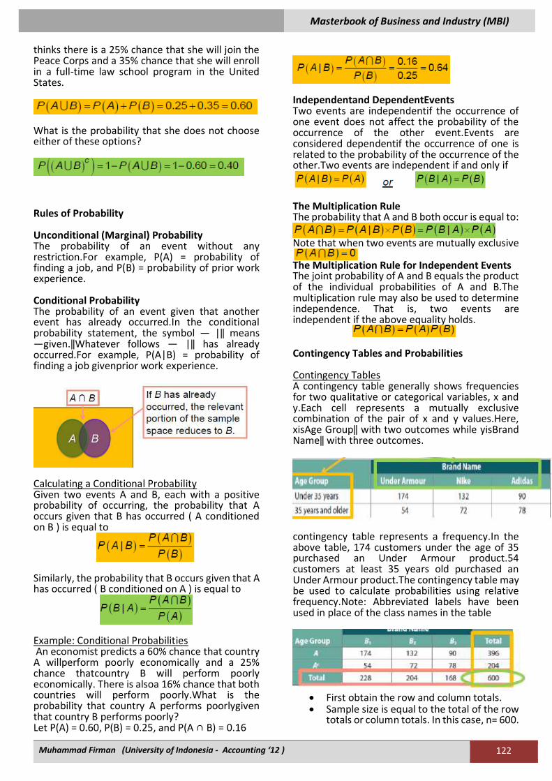
Rules of Probability Unconditional (Marginal) Probability The probability of an event without any restriction.For example, P(A) = probability of finding a job, and P(B) = probability of prior work experience. Conditional Probability The probability of an event given that another event has already occurred.In the conditional probability statement, the symbol ― |‖ means ―given.‖Whatever follows ― |‖ has already occurred.For example, P(A|B) = probability of finding a job givenprior work experience.
Calculating a Conditional Probability Given two events A and B, each with a positive probability of occurring, the probability that A occurs given that B has occurred ( A conditioned on B ) is equal to
Similarly, the probability that B occurs given that A has occurred ( B conditioned on A ) is equal to
Example: Conditional Probabilities An economist predicts a 60% chance that country A willperform poorly economically and a 25% chance thatcountry B will perform poorly economically. There is alsoa 16% chance that both countries will perform poorly.What is the probability that country A performs poorlygiven that country B performs poorly? Let P(A) = 0.60, P(B) = 0.25, and P(A ∩ B) = 0.16
Independentand DependentEvents Two events are independentif the occurrence of one event does not affect the probability of the occurrence of the other event.Events are considered dependentif the occurrence of one is related to the probability of the occurrence of the other.Two events are independent if and only if
The Multiplication Rule The probability that A and B both occur is equal to:
Note that when two events are mutually exclusive
The Multiplication Rule for Independent Events The joint probability of A and B equals the product of the individual probabilities of A and B.The multiplication rule may also be used to determine independence. That is, two events are independent if the above equality holds.
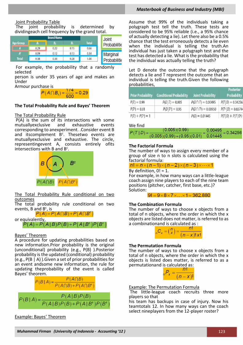
Contingency Tables and Probabilities Contingency Tables A contingency table generally shows frequencies for two qualitative or categorical variables, x and y.Each cell represents a mutually exclusive combination of the pair of x and y values.Here, xisAge Group‖ with two outcomes while yisBrand Name‖ with three outcomes.
contingency table represents a frequency.In the above table, 174 customers under the age of 35 purchased an Under Armour product.54 customers at least 35 years old purchased an Under Armour product.The contingency table may be used to calculate probabilities using relative frequency.Note: Abbreviated labels have been used in place of the class names in the table
• First obtain the row and column totals. • Sample size is equal to the total of the row
totals or column totals. In this case, n= 600.
Masterbook of Business and Industry (MBI)
Muhammad Firman (University of Indonesia - Accounting ‘12 ) 123
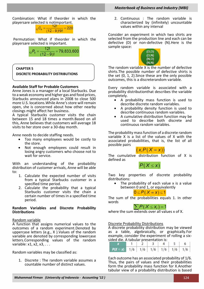
Joint Probability Table The joint probability is determined by dividingeach cell frequency by the grand total.
For example, the probability that a randomly selected person is under 35 years of age and makes an Under Armour purchase is
The Total Probability Rule and Bayes’ Theorem The Total Probability Rule P(A) is the sum of its intersections with some mutuallyexclusive and exhaustive events corresponding to anexperiment. .Consider event B and itscomplement Bc. Thesetwo events are mutuallyexclusive and exhaustive. The circle, representingevent A, consists entirely ofits intersections with B and Bc.
The Total Probability Rule conditional on two outcomes The total probability rule conditional on two events, B and Bc, is
or equivalently,
Bayes’ Theorem A procedure for updating probabilities based on new information.Prior probability is the original (unconditional) probability (e.g., P(B) ).Posterior probability is the updated (conditional) probability (e.g., P(B | A) ).Given a set of prior probabilities for an event andsome new information, the rule for updating theprobability of the event is called Bayes’ theorem.
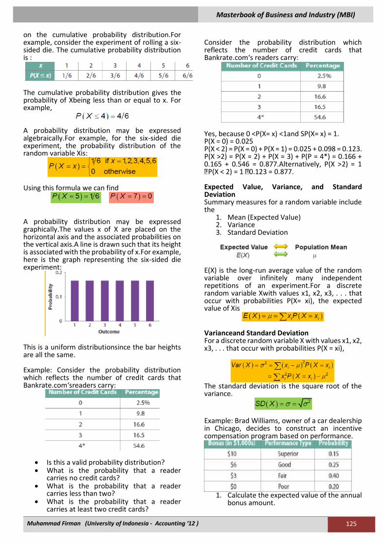
Example: Bayes‘ Theorem
Assume that 99% of the individuals taking a polygraph test tell the truth. These tests are considered to be 95% reliable (i.e., a 95% chance of actually detecting a lie). Let there also be a 0.5% chance that the test erroneously detects a lie even when the individual is telling the truth.An individual has just taken a polygraph test and the test has detected a lie. What is the probability that the individual was actually telling the truth? Let D denote the outcome that the polygraph detects a lie and T represent the outcome that an individual is telling the truth.Given the following probabilities,
We find
The Factorial Formula The number of ways to assign every member of a group of size n to n slots is calculated using the factorial formula:
By definition, 0! = 1. For example, in how many ways can a little-league coach assign nine players to each of the nine team positions (pitcher, catcher, first base, etc.)? Solution:
The Combination Formula The number of ways to choose x objects from a total of n objects, where the order in which the x objects are listed does not matter, is referred to as a combinationand is calculated as :
The Permutation Formula The number of ways to choose x objects from a total of n objects, where the order in which the x objects is listed does matter, is referred to as a permutationand is calculated as:
Example: The Permutation Formula The little-league coach recruits three more players so that his team has backups in case of injury. Now his teamtotals 12. In how many ways can the coach select nineplayers from the 12-player roster?
Masterbook of Business and Industry (MBI)
Muhammad Firman (University of Indonesia - Accounting ‘12 ) 124
Combination: What if theorder in which the playersare selected is notimportant.
Permutation: What if theorder in which the playersare selected is important.
Available Staff for Probable Customers Anne Jones is a manager of a local Starbucks. Due to a weak economy and higher gas and food prices, Starbucks announced plans in 2008 to close 500 more U.S. locations.While Anne‘s store will remain open, she is concerned about how other nearby closings might affect her business. A typical Starbucks customer visits the chain between 15 and 18 times a month.Based on all this, Anne believes that customers will average 18 visits to her store over a 30-day month. Anne needs to decide staffing needs.
• Too many employees would be costly to the store.
• Not enough employees could result in losing angry customers who choose not to wait for service.
With an understanding of the probability distribution of customer arrivals, Anne will be able to:
1. Calculate the expected number of visits from a typical Starbucks customer in a specified time period.
2. Calculate the probability that a typical Starbucks customer visits the chain a certain number of times in a specified time period.
Random Variables and Discrete Probability Distributions Random variable A function that assigns numerical values to the outcomes of a random experiment.Denoted by uppercase letters (e.g., X ).Values of the random variable are denoted by corresponding lowercase letters.Corresponding values of the random variable: x1, x2, x3, . . . Random variables may be classified as:
1. Discrete : The random variable assumes a countable number of distinct values.
2. Continuous : The random variable is characterized by (infinitely) uncountable values within any interval
Consider an experiment in which two shirts are selected from the production line and each can be defective (D) or non-defective (N).Here is the sample space:
The random variable X is the number of defective shirts.The possible number of defective shirts is the set {0, 1, 2}.Since these are the only possible outcomes, this is a discreterandom variable. Every random variable is associated with a probability distributionthat describes the variable completely.
• A probability mass function is used to describe discrete random variables.
• A probability density function is used to describe continuous random variables.
• A cumulative distribution function may be used to describe both discrete and continuous random variables.
The probability mass function of a discrete random variable X is a list of the values of X with the associated probabilities, that is, the list of all possible pairs
The cumulative distribution function of X is defined as
Two key properties of discrete probability distributions:
• The probability of each value x is a value between 0 and 1, or equivalently
The sum of the probabilities equals 1. In other words
where the sum extends over all values x of X. Discrete Probability Distributions A discrete probability distribution may be viewed as a table, algebraically, or graphically.For example, consider the experiment of rolling a six-sided die. A tabular presentation is:
Each outcome has an associated probability of 1/6. Thus, the pairs of values and their probabilities form the probability mass function for X.Another tabular view of a probability distribution is based
CHAPTER 5
DISCRETE PROBABILITY DISTRIBUTIONS
Masterbook of Business and Industry (MBI)
Muhammad Firman (University of Indonesia - Accounting ‘12 ) 125
on the cumulative probability distribution.For example, consider the experiment of rolling a six-sided die. The cumulative probability distribution is :
The cumulative probability distribution gives the probability of Xbeing less than or equal to x. For example,
A probability distribution may be expressed algebraically.For example, for the six-sided die experiment, the probability distribution of the random variable Xis:
Using this formula we can find
A probability distribution may be expressed graphically.The values x of X are placed on the horizontal axis and the associated probabilities on the vertical axis.A line is drawn such that its height is associated with the probability of x.For example, here is the graph representing the six-sided die experiment:
This is a uniform distributionsince the bar heights are all the same. Example: Consider the probability distribution which reflects the number of credit cards that Bankrate.com‘sreaders carry:
• Is this a valid probability distribution? • What is the probability that a reader
carries no credit cards? • What is the probability that a reader
carries less than two? • What is the probability that a reader
carries at least two credit cards?
Consider the probability distribution which reflects the number of credit cards that Bankrate.com‘s readers carry:
Yes, because 0 <P(X= x) <1and SP(X= x) = 1. P(X = 0) = 0.025 P(X < 2) = P(X = 0) + P(X = 1) = 0.025 + 0.098 = 0.123. P(X >2) = P(X = 2) + P(X = 3) + P(P = 4*) = 0.166 + 0.165 + 0.546 = 0.877.Alternatively, P(X >2) = 1
P(X < 2) = 1 0.123 = 0.877. Expected Value, Variance, and Standard Deviation Summary measures for a random variable include the
1. Mean (Expected Value) 2. Variance 3. Standard Deviation
E(X) is the long-run average value of the random variable over infinitely many independent repetitions of an experiment.For a discrete random variable Xwith values x1, x2, x3, . . . that occur with probabilities P(X= xi), the expected value of Xis
Varianceand Standard Deviation For a discrete random variable X with values x1, x2, x3, . . . that occur with probabilities P(X = xi),
The standard deviation is the square root of the variance.
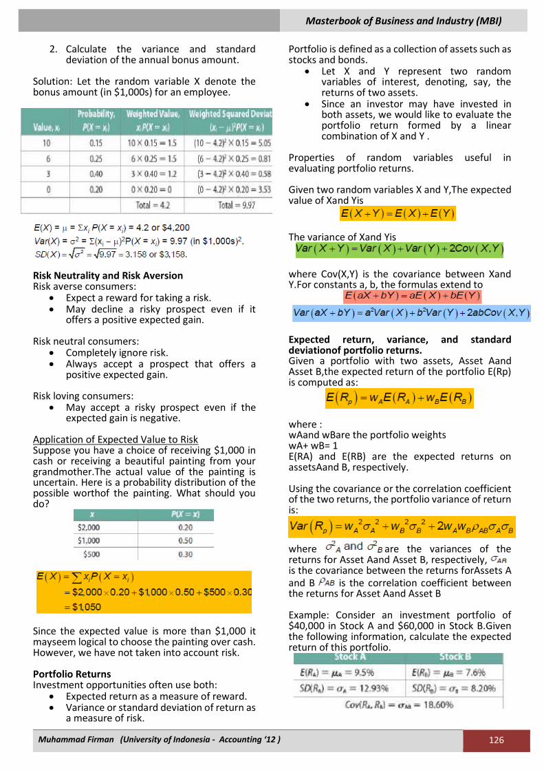
Example: Brad Williams, owner of a car dealership in Chicago, decides to construct an incentive compensation program based on performance.
1. Calculate the expected value of the annual
bonus amount.
Masterbook of Business and Industry (MBI)
Muhammad Firman (University of Indonesia - Accounting ‘12 ) 126
2. Calculate the variance and standard deviation of the annual bonus amount.
Solution: Let the random variable X denote the bonus amount (in $1,000s) for an employee.
Risk Neutrality and Risk Aversion Risk averse consumers:
• Expect a reward for taking a risk. • May decline a risky prospect even if it
offers a positive expected gain. Risk neutral consumers:
• Completely ignore risk. • Always accept a prospect that offers a
positive expected gain. Risk loving consumers:
• May accept a risky prospect even if the expected gain is negative.
Application of Expected Value to Risk Suppose you have a choice of receiving $1,000 in cash or receiving a beautiful painting from your grandmother.The actual value of the painting is uncertain. Here is a probability distribution of the possible worthof the painting. What should you do?
Since the expected value is more than $1,000 it mayseem logical to choose the painting over cash. However, we have not taken into account risk. Portfolio Returns Investment opportunities often use both:
• Expected return as a measure of reward. • Variance or standard deviation of return as
a measure of risk.
Portfolio is defined as a collection of assets such as stocks and bonds.
• Let X and Y represent two random variables of interest, denoting, say, the returns of two assets.
• Since an investor may have invested in both assets, we would like to evaluate the portfolio return formed by a linear combination of X and Y .
Properties of random variables useful in evaluating portfolio returns. Given two random variables X and Y,The expected value of Xand Yis
The variance of Xand Yis
where Cov(X,Y) is the covariance between Xand Y.For constants a, b, the formulas extend to
Expected return, variance, and standard deviationof portfolio returns. Given a portfolio with two assets, Asset Aand Asset B,the expected return of the portfolio E(Rp) is computed as:
where : wAand wBare the portfolio weights wA+ wB= 1 E(RA) and E(RB) are the expected returns on assetsAand B, respectively. Using the covariance or the correlation coefficient of the two returns, the portfolio variance of return is:
where are the variances of the returns for Asset Aand Asset B, respectively, is the covariance between the returns forAssets A and B is the correlation coefficient between the returns for Asset Aand Asset B Example: Consider an investment portfolio of $40,000 in Stock A and $60,000 in Stock B.Given the following information, calculate the expected return of this portfolio.
Masterbook of Business and Industry (MBI)
Muhammad Firman (University of Indonesia - Accounting ‘12 ) 127
Example: Consider an investment portfolio of $40,000 in Stock A and $60,000 in Stock B.
Calculate the correlation coefficient between the returns on Stocks A and B.Solution:
Calculate the portfolio variance. Solution:
Calculate the portfolio standard deviation. Solution:
The Binomial Probability Distribution A binomial random variable is defined as the number of successes achieved in the n trials of a Bernoulli process.A Bernoulli process consists of a series of n independent and identical trials of an experiment such that on each trial: There are only two possible outcomes:
• p = probability of a success • 1-p = q = probability of a failure
Each time the trial is repeated, the probabilities of success and failure remain the same. A binomial random variable X is defined as the number of successes achieved in the n trials of a Bernoulli process.A binomial probability distribution shows the probabilities associated with the possible values of the binomial random variable (that is, 0, 1, . . . , n).For a binomial random variable X , the probability of x successes in n Bernoulli trials is
For a binomial distribution: The expected value (E(X)) is:
The variance(Var(X)) is:
The standard deviation (SD(X)) is:
Example: Approximately 20% of U.S. workers are afraid that they will never be able to retire. Suppose 10 workers are randomly selected.What is the probability that none of the workers is afraid that they will never be able to retire? Solution: Let X= 10, then
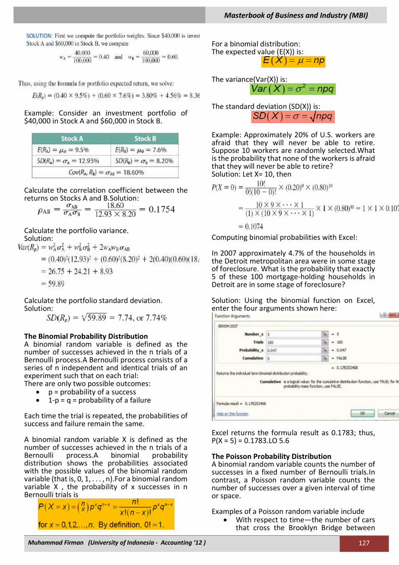
Computing binomial probabilities with Excel: In 2007 approximately 4.7% of the households in the Detroit metropolitan area were in some stage of foreclosure. What is the probability that exactly 5 of these 100 mortgage-holding households in Detroit are in some stage of foreclosure? Solution: Using the binomial function on Excel, enter the four arguments shown here:
Excel returns the formula result as 0.1783; thus, P(X = 5) = 0.1783.LO 5.6 The Poisson Probability Distribution A binomial random variable counts the number of successes in a fixed number of Bernoulli trials.In contrast, a Poisson random variable counts the number of successes over a given interval of time or space. Examples of a Poisson random variable include
• With respect to time—the number of cars that cross the Brooklyn Bridge between
Masterbook of Business and Industry (MBI)
Muhammad Firman (University of Indonesia - Accounting ‘12 ) 128
9:00 am and 10:00 am on a Monday morning.
• With respect to space—the number of defects in a 50-yard roll of fabric.
A random experiment satisfies a Poisson process if:
1. The number of successes within a specified time or space interval equals any integer between zero and infinity.
2. The numbers of successes counted in nonoverlapping intervals are independent.
3. The probability that success occurs in any interval is the same for all intervals of equal size and is proportional to the size of the interval.
For a Poisson random variable X, the probability of x successes over a given interval of time or space is
where is the mean number of successes and e
2.718 is the base of the natural logarithm. For a Poisson distribution:
The expected value (E(X)) is:
The variance (Var(X)) is: The standard deviation(SD(X)) is:
Example: Returning to the Starbucks example, Ann believes that the typical Starbucks customer averages 18 visits over a 30-day month.How many visits should Anne expect in a 5-day period from a typical Starbucks customer?
What is the probability that a customer visits the chain five times in a 5-day period?
The Hypergeometric Probability Distribution A binomial random variable X is defined as the number of successes in the n trials of a Bernoulli process, and according to a Bernoulli process, those trials are
1. Independent 2. The probability of success does not change
from trial to trial. In contrast, the hypergeometric probability distribution is appropriate in applications where we cannot assume the trials are independent.Use
the hypergeometric distribution when sampling without replacement from a population whose size N is not significantly larger than the sample size n.For a hypergeometric random variable X, the probability of x successes in a random selection of n items is
where Ndenotes the number of items in the population of which Sare successes For a hypergeometric distribution: The expected value (E(X)) is:
The variance (Var(X))is:
The standard deviation(SD(X)) is:
Example: At a convenience store in Morganville, New Jersey, the manager randomly inspects five mangoes from a box containing 20 mangoes for damages due to transportation. Suppose the chosen box contains exactly 2 damaged mangoes.What is the probability that one out of five mangoes used in the inspection are damaged?
Demand for Salmon Akiko Hamaguchi, manager of a small sushi restaurant, Little Ginza, in Phoenix, Arizona, has to estimate the daily amount of salmon needed.Akiko has estimated the daily consumption of salmon to be normally distributed with a mean of 12 pounds and a standard deviation of 3.2 pounds.Buying 20 lbs of salmon every day has resulted in too much wastage.Therefore, Akiko will buy salmon that meets the daily demand of customers on 90% of the days. Based on this information, Akiko would like to:
CHAPTER 6
CONTINUOUS PROBABILITY DISTRIBUTIONS
Masterbook of Business and Industry (MBI)
Muhammad Firman (University of Indonesia - Accounting ‘12 ) 129
1. Calculate the proportion of days that demand for salmon at Little Ginza was above her earlier purchase of 20 pounds.
2. Calculate the proportion of days that demand for salmon at Little Ginza was below 15 pounds.
3. Determine the amount of salmon that should be bought daily so that it meets demand on 90% of the days.
Continuous Random Variables and the Uniform Probability Distribution Remember that random variables may be classified as Discrete : The random variable assumes a countable number of distinct values. Continuous : The random variable is characterized by (infinitely) uncountable values within any interval. When computing probabilities for a continuous random variable, keep in mind that P(X= x) = 0.We cannot assign a nonzero probability to each infinitely uncountable value and still have the probabilities sum to one.Thus, since P(X= a) and P(X= b) both equal zero, the following holds for continuous random variables:
Probability Density Functionf(x) Probability Density Functionf(x) of a continuous random variable XDescribes the relative likelihood that X assumes a value within a given interval (e.g., P(a <X <b) ), where
• f(x) > 0 for all possible values of X. • The area under f(x) over all values of
xequals one. Cumulative Density Function F(x) Cumulative Density Function F(x)of a continuous random variable XFor any value x of the random variable X, the cumulative distribution function F(x) is computed as
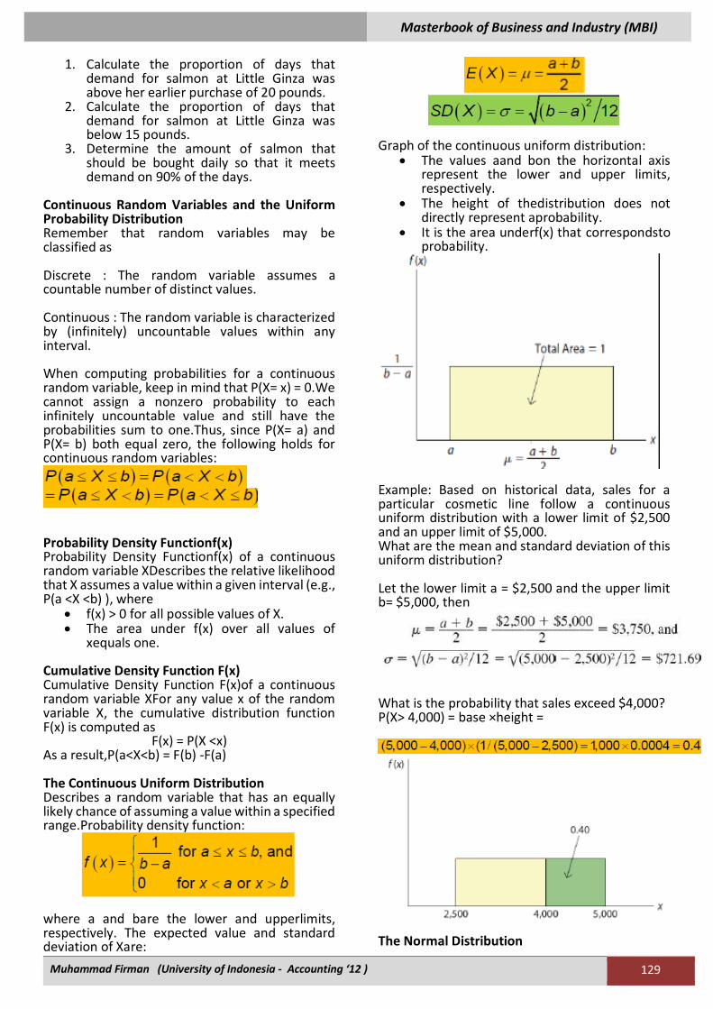
F(x) = P(X <x) As a result,P(a<X<b) = F(b) -F(a) The Continuous Uniform Distribution Describes a random variable that has an equally likely chance of assuming a value within a specified range.Probability density function:
where a and bare the lower and upperlimits, respectively. The expected value and standard deviation of Xare:
Graph of the continuous uniform distribution:
• The values aand bon the horizontal axis represent the lower and upper limits, respectively.
• The height of thedistribution does not directly represent aprobability.
• It is the area underf(x) that correspondsto probability.
Example: Based on historical data, sales for a particular cosmetic line follow a continuous uniform distribution with a lower limit of $2,500 and an upper limit of $5,000. What are the mean and standard deviation of this uniform distribution? Let the lower limit a = $2,500 and the upper limit b= $5,000, then
What is the probability that sales exceed $4,000? P(X> 4,000) = base ×height =
The Normal Distribution
Masterbook of Business and Industry (MBI)
Muhammad Firman (University of Indonesia - Accounting ‘12 ) 130
1. Symmetric 2. Bell-shaped
Closely approximates the probability distribution of a wide range of random variables, such as the
• Heights and weights of newborn babies • Scores on SAT • Cumulative debt of college graduates
Serves as the cornerstone of statistical inference. Characteristics of the Normal Distribution Symmetricabout its mean Mean = Median = Mode Asymptotic—that is, the tails get closer and closer to the horizontal axis, but never touch it
The normal distribution is completely described by
two parameters: .
is the population mean which describes the central location of the distribution.
is the population variance which describes the dispersion of the distribution. Probability Density Function of the Normal Distribution For a random variable X with mean mand variance
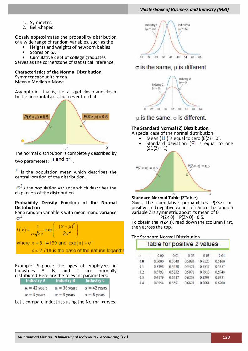
Example: Suppose the ages of employees in Industries A, B, and C are normally distributed.Here are the relevant parameters:
Let‘s compare industries using the Normal curves.
The Standard Normal (Z) Distribution. A special case of the normal distribution:
• Mean ( ) is equal to zero (E(Z) = 0). • Standard deviation ( is equal to one
(SD(Z) = 1)
Standard Normal Table (ZTable). Gives the cumulative probabilities P(Z<z) for positive and negative values of z.Since the random variable Z is symmetric about its mean of 0,
P(Z< 0) = P(Z> 0)= 0.5. To obtain the P(Z< z), read down the zcolumn first, then across the top. The Standard Normal Distribution
Masterbook of Business and Industry (MBI)
Muhammad Firman (University of Indonesia - Accounting ‘12 ) 131
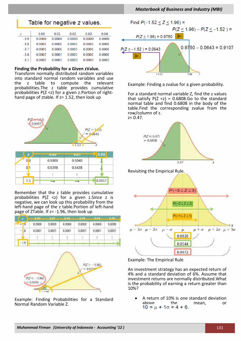
Finding the Probability for a Given zValue. Transform normally distributed random variables into standard normal random variables and use the z table to compute the relevant probabilities.The z table provides cumulative probabilities P(Z <z) for a given z.Portion of right-hand page of ztable. If z= 1.52, then look up
Remember that the z table provides cumulative probabilities P(Z <z) for a given z.Since z is negative, we can look up this probability from the left-hand page of the z table.Portion of left-hand page of ZTable. If z= -1.96, then look up
Example: Finding Probabilities for a Standard Normal Random Variable Z.
Example: Finding a zvalue for a given probability. For a standard normal variable Z, find the z values that satisfy P(Z <z) = 0.6808.Go to the standard normal table and find 0.6808 in the body of the table.Find the corresponding zvalue from the row/column of z. z= 0.47.
Revisiting the Empirical Rule.
Example: The Empirical Rule An investment strategy has an expected return of 4% and a standard deviation of 6%. Assume that investment returns are normally distributed.What is the probability of earning a return greater than 10%?
• A return of 10% is one standard deviation above the mean, or
Masterbook of Business and Industry (MBI)
Muhammad Firman (University of Indonesia - Accounting ‘12 ) 132
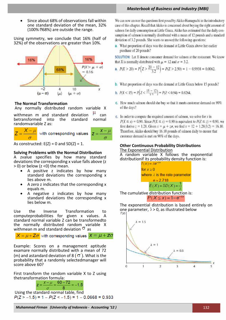
• Since about 68% of observations fall within one standard deviation of the mean, 32% (100% 68%) are outside the range.
Using symmetry, we conclude that 16% (half of 32%) of the observations are greater than 10%.
The Normal Transformation Any normally distributed random variable X
withmean m and standard deviation can betransformed into the standard normal randomvariable Z as:
As constructed: E(Z) = 0 and SD(Z) = 1. Solving Problems with the Normal Distribution A zvalue specifies by how many standard deviations the corresponding x value falls above (z > 0) or below (z <0) the mean.
• A positive z indicates by how many standard deviations the corresponding x lies above m.
• A zero z indicates that the corresponding x equals m.
• A negative z indicates by how many standard deviations the corresponding x lies below m.
Use the Inverse Transformation to computeprobabilities for given x values. A standard normal variable Z can be transformedto the normally distributed random variable X withmean m and standard deviation as
Example: Scores on a management aptitude examare normally distributed with a mean of 72 (m) and astandard deviation of 8 ( ). What is the probability that a randomly selectedmanager will score above 60? First transform the random variable X to Z using thetransformation formula:
Using the standard normal table, find
Other Continuous Probability Distributions The Exponential Distribution A random variable X follows the exponential distributionif its probability density function is:
The cumulative dIstribution function is:
The exponential distribution is based entirely on one parameter, > 0, as illustrated below
Masterbook of Business and Industry (MBI)
Muhammad Firman (University of Indonesia - Accounting ‘12 ) 133
The Lognormal Distribution Defined for a positive random variable, the lognormal distribution is positively skewed.Useful for describing variables such as :
1. Income 2. Real estate values 3. Asset prices
Failure rate may increase or decrease over time. Let X be a normally distributed random variable with mean and standard deviation The random variable Y = eXfollows the lognormal distribution with a probability density function as :
The graphs below show the shapes of the lognormal density function based on various values of
The lognormal distribution is clearly positively skewed for >1. For <1, the lognormal distribution somewhat resembles the normal distribution.
Expected values and standard deviations ofthe lognormal and normal distributions. Let X be a normal random variable withmean mand standard deviation and let Y = eX be thecorresponding
lognormal variable. The mean and standard
deviation of Y are derived as
Expected values and standard deviations ofthe lognormal and normal distributions. Equivalently, the mean and standard deviation ofthe normal variable X = ln(Y) are derived as
Marketing Iced Coffee In order to capitalize on the iced coffee trend, Starbucks offered for a limited time half-priced Frappuccino beverages between 3 pm and 5 pm.Anne Jones, manager at a local Starbucks, determines the following from past historical data:
• 43% of iced-coffee customers were women.
• 21% were teenage girls. • Customers spent an average of $4.18 on
iced coffee with a standard deviation of $0.84.
CHAPTER 7
SAMPLING AND SAMPLING DISTRIBUTIONS
Masterbook of Business and Industry (MBI)
Muhammad Firman (University of Indonesia - Accounting ‘12 ) 134
One month after the marketing period ends, Anne surveys 50 of her iced-coffee customers and finds:
• 46% were women. • 34% were teenage girls. • They spent an average of $4.26 on the
drink. Anne wants to use this survey information to calculate the probability that:
• Customers spend an average of $4.26 or more on iced coffee.
• 46% or more of iced-coffee customers are women.
• 34% or more of iced-coffee customers are teenage girls.
Sampling Population—consists of all items of interest in a statistical problem.
• Population Parameter is unknown. Sample—a subset of the population.
• Sample Statisticis calculated from sample and used to make inferences about the population.
Bias—the tendency of a sample statistic to systematically over-or underestimate a population parameter. Classic Case of a ―Bad‖ Sample: The Literary Digest Debacle of 1936
• During the1936 presidential election, the Literary Digest predicted a landslide victory for Alf Landon over Franklin D. Roosevelt (FDR) with only a 1% margin of error.
• They were wrong! FDR won in a landslide election.
• The Literary Digest had committed selection biasby randomly sampling from their own subscriber/ membership lists, etc.
• In addition, with only a 24% response rate, the Literary Digest had a great deal of non-response bias.LO 7.2 Explain common sample biases.
Selection bias a systematic exclusion of certain groups from consideration for the sample.
• The Literary Digest committed selection bias by excluding a large portion of the population (e.g., lower income voters).
Nonresponse bias a systematic difference in preferences between respondents and non-respondents to a survey or a poll.
• The Literary Digesthad only a 24% response rate. This indicates that only those who cared a great deal about the election took the time to respond to the
survey. These respondents may be atypical of the population as a whole.
Sampling Methods Simple random sample is a sample of n observations which has the same probability of being selected from the population as any other sample of n observations.Most statistical methods presume simple random samples.However, in some situations other sampling methods have an advantage over simple random samples. Example: In 1961, students invested 24 hours per week in their academic pursuits, whereas today‘s students study an average of 14 hours per week.A dean at a large university in California wonders if this trend is reflective of the students at her university. The university has 20,000 students and the dean would like a sample of 100. Use Excel to draw a simple random sample of 100 students. In Excel, choose Formulas > Insert function > RANDBETWEEN and input the values shown here.
Stratified Random Sampling Divide the population into mutually exclusive and collectively exhaustive groups, called strata.Randomly select observations from each stratum, which are proportional to the stratum‘s size. Advantages:
1. Guarantees that the each population subdivision is represented in the sample.
2. Parameter estimates have greater precision than those estimated from simple random sampling.
Cluster Sampling Divide population into mutually exclusive and collectively exhaustive groups, called clusters.Randomly select clusters. Sample every observation in those randomly selected clusters. Advantages and disadvantages:
1. Less expensive than other sampling methods.
2. Less precision than simple random sampling or stratified sampling.
Masterbook of Business and Industry (MBI)
Muhammad Firman (University of Indonesia - Accounting ‘12 ) 135
3. Useful when clusters occur naturally in the population.
Stratified Sampling
1. Sample consists of elements from each group.
2. Preferred when the objective is to increase precision.
Cluster Sampling
1. Sample consists of elements from the selected groups.
2. Preferred when the objective is to reduce costs.
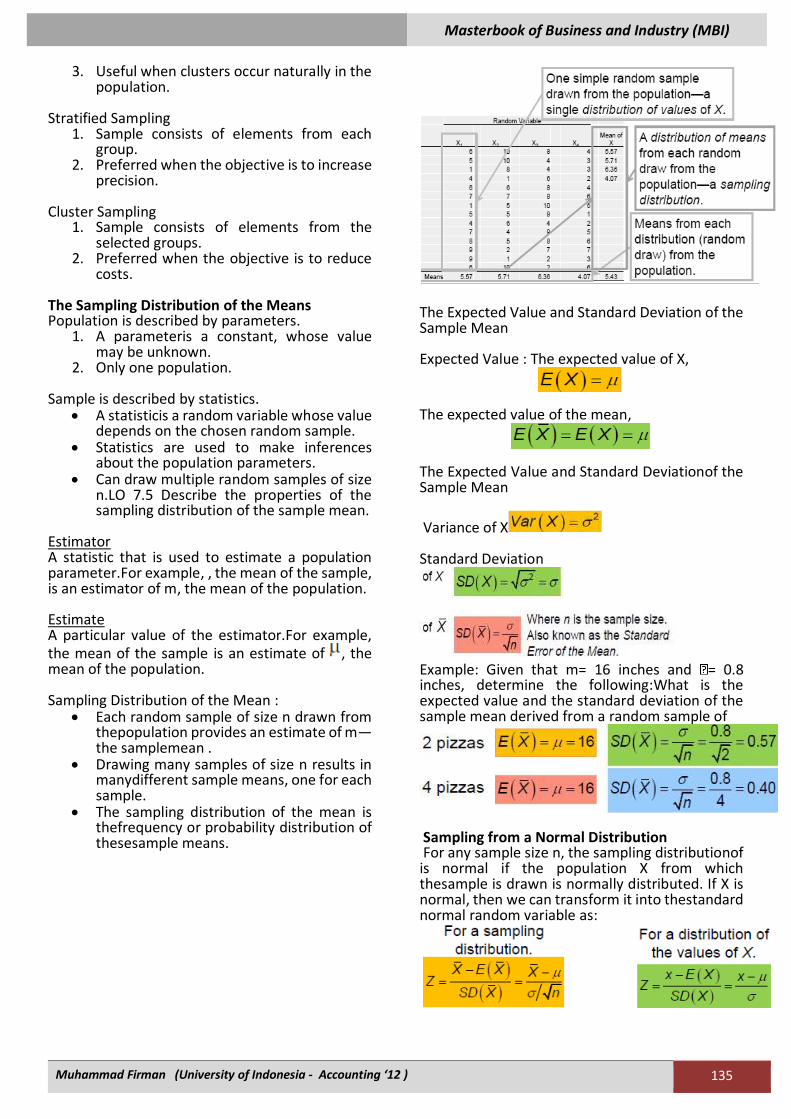
The Sampling Distribution of the Means Population is described by parameters.
1. A parameteris a constant, whose value may be unknown.
2. Only one population. Sample is described by statistics.
• A statisticis a random variable whose value depends on the chosen random sample.
• Statistics are used to make inferences about the population parameters.
• Can draw multiple random samples of size n.LO 7.5 Describe the properties of the sampling distribution of the sample mean.
Estimator A statistic that is used to estimate a population parameter.For example, , the mean of the sample, is an estimator of m, the mean of the population. Estimate A particular value of the estimator.For example, the mean of the sample is an estimate of , the mean of the population. Sampling Distribution of the Mean :
• Each random sample of size n drawn from thepopulation provides an estimate of m—the samplemean .
• Drawing many samples of size n results in manydifferent sample means, one for each sample.
• The sampling distribution of the mean is thefrequency or probability distribution of thesesample means.
The Expected Value and Standard Deviation of the Sample Mean Expected Value : The expected value of X,
The expected value of the mean,
The Expected Value and Standard Deviationof the Sample Mean
Variance of X Standard Deviation
Example: Given that m= 16 inches and = 0.8 inches, determine the following:What is the expected value and the standard deviation of the sample mean derived from a random sample of
Sampling from a Normal Distribution For any sample size n, the sampling distributionof is normal if the population X from which thesample is drawn is normally distributed. If X is normal, then we can transform it into thestandard normal random variable as:
Masterbook of Business and Industry (MBI)
Muhammad Firman (University of Indonesia - Accounting ‘12 ) 136
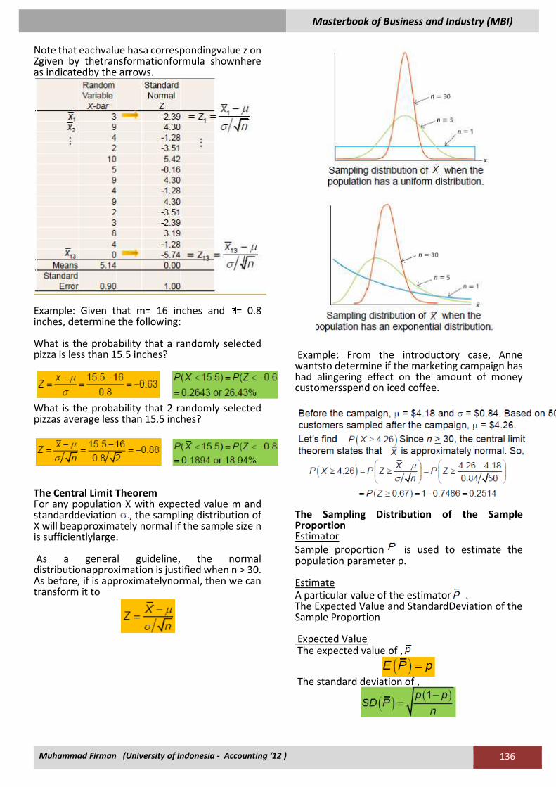
Note that eachvalue hasa correspondingvalue z on Zgiven by thetransformationformula shownhere as indicatedby the arrows.
Example: Given that m= 16 inches and = 0.8 inches, determine the following: What is the probability that a randomly selected pizza is less than 15.5 inches?
What is the probability that 2 randomly selected pizzas average less than 15.5 inches?
The Central Limit Theorem For any population X with expected value m and standarddeviation , the sampling distribution of X will beapproximately normal if the sample size n is sufficientlylarge. As a general guideline, the normal distributionapproximation is justified when n > 30. As before, if is approximatelynormal, then we can transform it to
Example: From the introductory case, Anne wantsto determine if the marketing campaign has had alingering effect on the amount of money customersspend on iced coffee.
The Sampling Distribution of the Sample Proportion Estimator Sample proportion is used to estimate the population parameter p. Estimate A particular value of the estimator . The Expected Value and StandardDeviation of the Sample Proportion Expected Value The expected value of ,
The standard deviation of ,
Masterbook of Business and Industry (MBI)
Muhammad Firman (University of Indonesia - Accounting ‘12 ) 137
The Central Limit Theorem for the Sample Proportion For any population proportion p, the sampling distribution of is approximately normal if the sample size n is sufficiently large .As a general guideline, the normal distribution approximation is justified when
If is normal, we can transform it into thestandard normal random variable as
Therefore any value on has a corresponding value z on Z given by
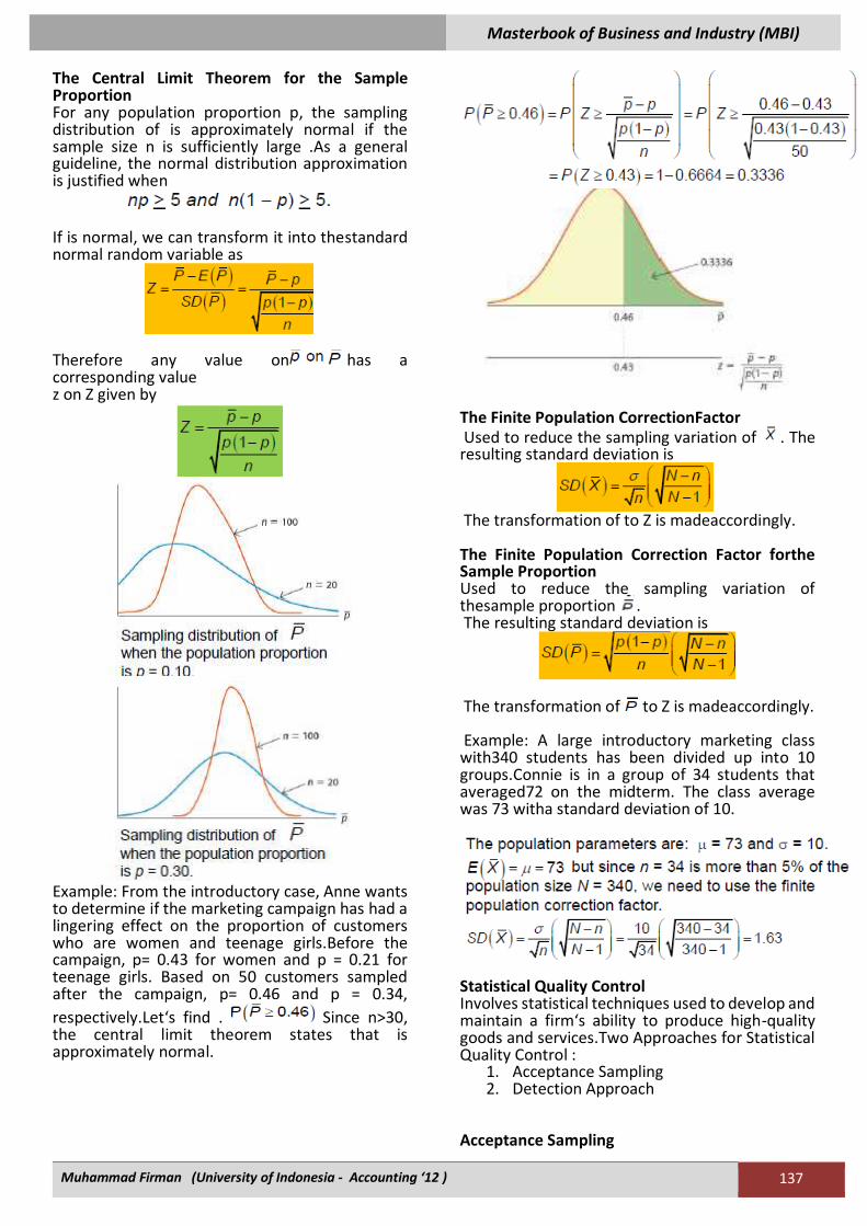
Example: From the introductory case, Anne wants to determine if the marketing campaign has had a lingering effect on the proportion of customers who are women and teenage girls.Before the campaign, p= 0.43 for women and p = 0.21 for teenage girls. Based on 50 customers sampled after the campaign, p= 0.46 and p = 0.34,
respectively.Let‘s find . Since n>30, the central limit theorem states that is approximately normal.
The Finite Population CorrectionFactor Used to reduce the sampling variation of . The resulting standard deviation is
The transformation of to Z is madeaccordingly. The Finite Population Correction Factor forthe Sample Proportion Used to reduce the sampling variation of thesample proportion . The resulting standard deviation is
The transformation of to Z is madeaccordingly. Example: A large introductory marketing class with340 students has been divided up into 10 groups.Connie is in a group of 34 students that averaged72 on the midterm. The class average was 73 witha standard deviation of 10.
Statistical Quality Control Involves statistical techniques used to develop and maintain a firm‘s ability to produce high-quality goods and services.Two Approaches for Statistical Quality Control :
1. Acceptance Sampling 2. Detection Approach
Acceptance Sampling
Masterbook of Business and Industry (MBI)
Muhammad Firman (University of Indonesia - Accounting ‘12 ) 138
Used at the completion of a production process or service.If a particular product does not conform to certain specifications, then it is either discarded or repaired. Disadvantages
1. It is costly to discard or repair a product. 2. The detection of all defective products is
not guaranteed.LO 7.9 Detection Approach Inspection occurs during the production process in order to detect any nonconformance to specifications.Goal is to determine whether the production process should be continued or adjusted before producing a large number of defects. Types of variation:
1. Chance variation. 2. Assignable variation.
Types of Variation Chance variation (common variation) is:
• Caused by a number of randomly occurring events that are part of the production process.
• Not controllable by the individual worker or machine.
• Expected, so not a source of alarm as long as its magnitude is tolerable and the end product meets specifications.
Assignable variation (special cause variation) is:
• Caused by specific events or factors that can usually be indentified and eliminated.
• Identified and corrected or removed. Control Charts A plot of calculated statistics of the production process over time.Production process is in control‖ if the calculated statistics fall in an expected range.Production process is out of control‖ if calculated statistics reveal an undesirable trend.
1. For quantitative data— chart.
2. For qualitative data— chart Control Charts for Quantitative Data
Control Charts • Centerline—the mean when the process is
under control. • Upper control limit—set at +3 from the
mean. • Points falling above the upper control limit
are considered to be out of control. • Lower control limit—set at −3 from the
mean. • Points falling below the lower control limit
are considered to be out of control.
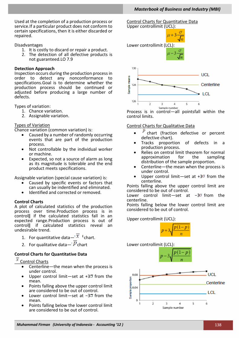
Control Charts for Quantitative Data Upper controllimit (UCL):
Lower controllimit (LCL):
Process is in control—all pointsfall within the control limits. Control Charts for Qualitative Data
• chart (fraction defective or percent defective chart).
• Tracks proportion of defects in a production process.
• Relies on central limit theorem for normal approximation for the sampling distribution of the sample proportion.
• Centerline—the mean when the process is under control.
• Upper control limit—set at +3 from the centerline.
Points falling above the upper control limit are considered to be out of control. Lower control limit—set at −3 from the centerline. Points falling below the lower control limit are considered to be out of control. Upper controllimit (UCL):
Lower controllimit (LCL):
Masterbook of Business and Industry (MBI)
Muhammad Firman (University of Indonesia - Accounting ‘12 ) 139
Process is out of controlsomepoints fall above the UCL.
Fuel Usage of “Ultra-Green” Cars A car manufacturer advertises that its new ―ultra-green‖ car obtains an average of 100 mpg and, based on its fuel emissions, has earned an A+ rating from the Environmental Protection Agency.Pinnacle Research, an independent consumer advocacy firm, obtains a sample of 25 cars for testing purposes.Each car is driven the same distance in identical conditions in order to obtain the car‘s mpg.The mpg for each ―Ultra-Green‖ car is given below.
Jared would like to use the data in this sample to: Estimate with 90% confidence
• The mean mpg of all ultra-green cars. • The proportion of all ultra-green cars that
obtain over 100 mpg. Determine the sample size needed to achieve a specified level of precision in the mean and proportion estimates. Point Estimators and Their Properties Point Estimator A function of the random sample used to make inferences about the value of an unknown population parameter.For example, is a point estimator for mand is a point estimator for p. Point Estimate The value of the point estimator derived from a given sample.For example, is a point estimate of the mean mpg for all ultra-green cars. Example:
Properties of Point Estimators
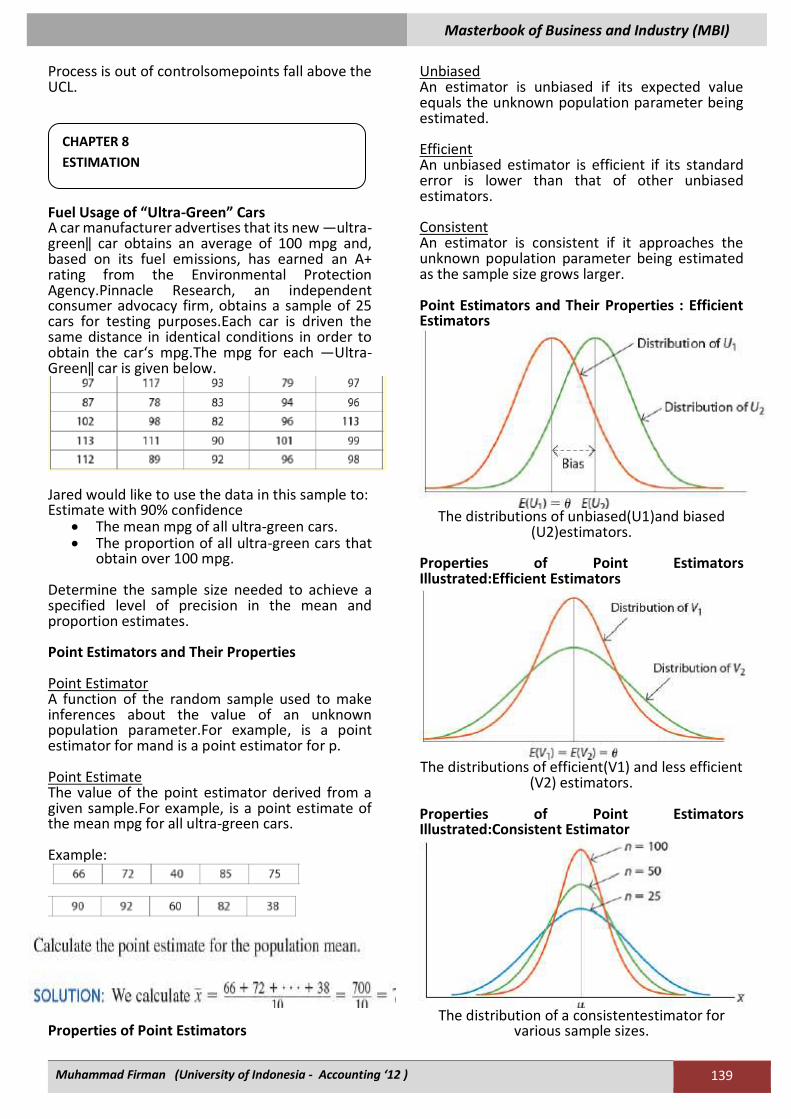
Unbiased An estimator is unbiased if its expected value equals the unknown population parameter being estimated. Efficient An unbiased estimator is efficient if its standard error is lower than that of other unbiased estimators. Consistent An estimator is consistent if it approaches the unknown population parameter being estimated as the sample size grows larger. Point Estimators and Their Properties : Efficient Estimators
The distributions of unbiased(U1)and biased
(U2)estimators. Properties of Point Estimators Illustrated:Efficient Estimators
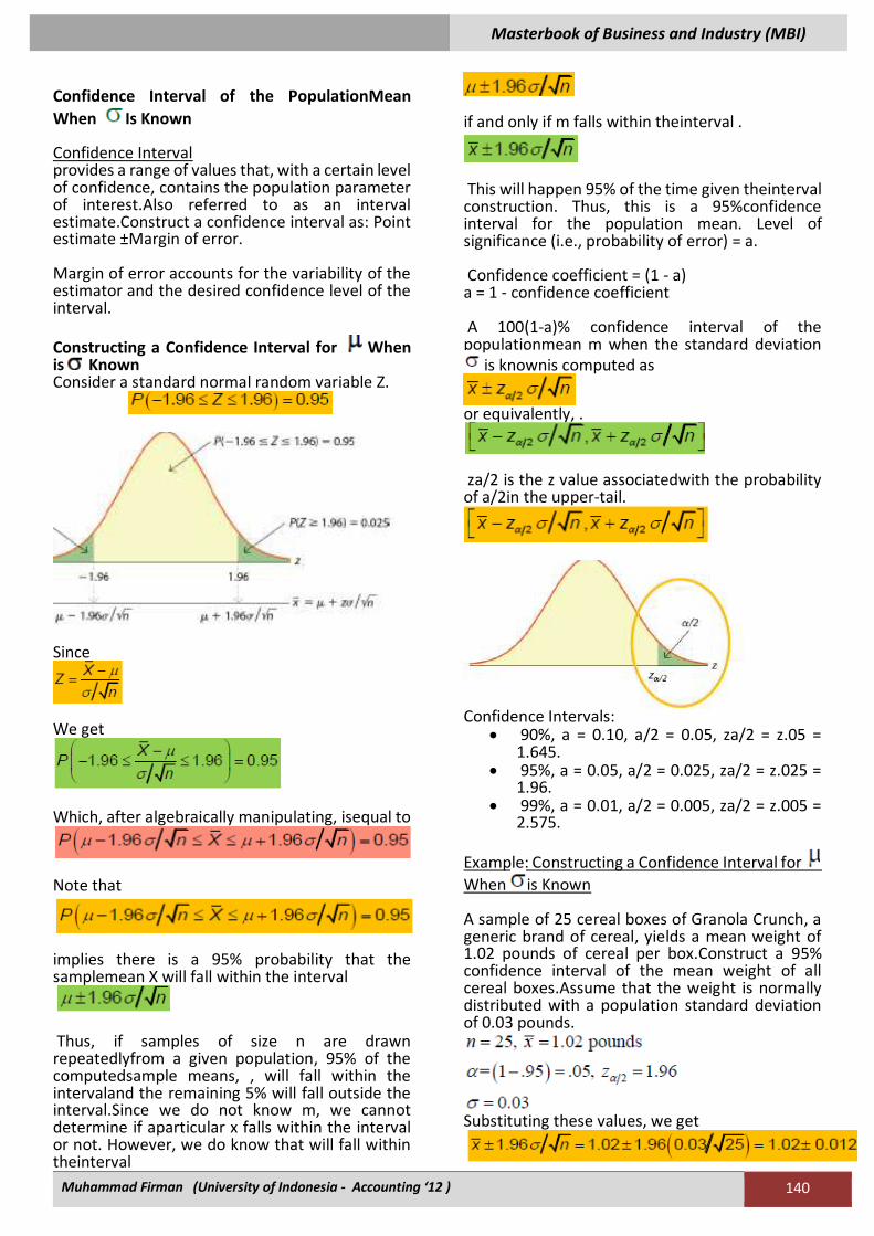
The distributions of efficient(V1) and less efficient
(V2) estimators. Properties of Point Estimators Illustrated:Consistent Estimator
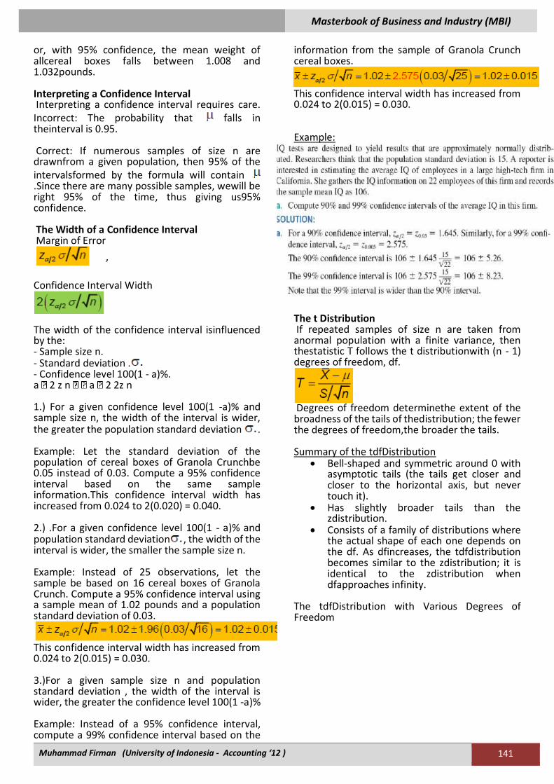
The distribution of a consistentestimator for
various sample sizes.
CHAPTER 8
ESTIMATION
Masterbook of Business and Industry (MBI)
Muhammad Firman (University of Indonesia - Accounting ‘12 ) 140
Confidence Interval of the PopulationMean
When Is Known Confidence Interval provides a range of values that, with a certain level of confidence, contains the population parameter of interest.Also referred to as an interval estimate.Construct a confidence interval as: Point estimate ±Margin of error. Margin of error accounts for the variability of the estimator and the desired confidence level of the interval.
Constructing a Confidence Interval for When is Known Consider a standard normal random variable Z.
Since
We get
Which, after algebraically manipulating, isequal to
Note that
implies there is a 95% probability that the samplemean X will fall within the interval
Thus, if samples of size n are drawn repeatedlyfrom a given population, 95% of the computedsample means, , will fall within the intervaland the remaining 5% will fall outside the interval.Since we do not know m, we cannot determine if aparticular x falls within the interval or not. However, we do know that will fall within theinterval
if and only if m falls within theinterval .
This will happen 95% of the time given theinterval construction. Thus, this is a 95%confidence interval for the population mean. Level of significance (i.e., probability of error) = a. Confidence coefficient = (1 - a) a = 1 - confidence coefficient A 100(1-a)% confidence interval of the populationmean m when the standard deviation
is knownis computed as
or equivalently, .
za/2 is the z value associatedwith the probability of a/2in the upper-tail.
Confidence Intervals:
• 90%, a = 0.10, a/2 = 0.05, za/2 = z.05 = 1.645.
• 95%, a = 0.05, a/2 = 0.025, za/2 = z.025 = 1.96.
• 99%, a = 0.01, a/2 = 0.005, za/2 = z.005 = 2.575.
Example: Constructing a Confidence Interval for
When is Known A sample of 25 cereal boxes of Granola Crunch, a generic brand of cereal, yields a mean weight of 1.02 pounds of cereal per box.Construct a 95% confidence interval of the mean weight of all cereal boxes.Assume that the weight is normally distributed with a population standard deviation of 0.03 pounds.
Substituting these values, we get
Masterbook of Business and Industry (MBI)
Muhammad Firman (University of Indonesia - Accounting ‘12 ) 141
or, with 95% confidence, the mean weight of allcereal boxes falls between 1.008 and 1.032pounds. Interpreting a Confidence Interval Interpreting a confidence interval requires care. Incorrect: The probability that falls in theinterval is 0.95. Correct: If numerous samples of size n are drawnfrom a given population, then 95% of the intervalsformed by the formula will contain .Since there are many possible samples, wewill be right 95% of the time, thus giving us95% confidence. The Width of a Confidence Interval Margin of Error
’ Confidence Interval Width
The width of the confidence interval isinfluenced by the: - Sample size n. - Standard deviation . - Confidence level 100(1 - a)%. a 2 z n a 2 2z n 1.) For a given confidence level 100(1 -a)% and sample size n, the width of the interval is wider, the greater the population standard deviation . Example: Let the standard deviation of the population of cereal boxes of Granola Crunchbe 0.05 instead of 0.03. Compute a 95% confidence interval based on the same sample information.This confidence interval width has increased from 0.024 to 2(0.020) = 0.040. 2.) .For a given confidence level 100(1 - a)% and population standard deviation , the width of the interval is wider, the smaller the sample size n. Example: Instead of 25 observations, let the sample be based on 16 cereal boxes of Granola Crunch. Compute a 95% confidence interval using a sample mean of 1.02 pounds and a population standard deviation of 0.03.
This confidence interval width has increased from 0.024 to 2(0.015) = 0.030. 3.)For a given sample size n and population standard deviation , the width of the interval is wider, the greater the confidence level 100(1 -a)% Example: Instead of a 95% confidence interval, compute a 99% confidence interval based on the
information from the sample of Granola Crunch cereal boxes.
This confidence interval width has increased from 0.024 to 2(0.015) = 0.030. Example:
The t Distribution If repeated samples of size n are taken from anormal population with a finite variance, then thestatistic T follows the t distributionwith (n - 1) degrees of freedom, df.
Degrees of freedom determinethe extent of the broadness of the tails of thedistribution; the fewer the degrees of freedom,the broader the tails. Summary of the tdfDistribution
• Bell-shaped and symmetric around 0 with asymptotic tails (the tails get closer and closer to the horizontal axis, but never touch it).
• Has slightly broader tails than the zdistribution.
• Consists of a family of distributions where the actual shape of each one depends on the df. As dfincreases, the tdfdistribution becomes similar to the zdistribution; it is identical to the zdistribution when dfapproaches infinity.
The tdfDistribution with Various Degrees of Freedom
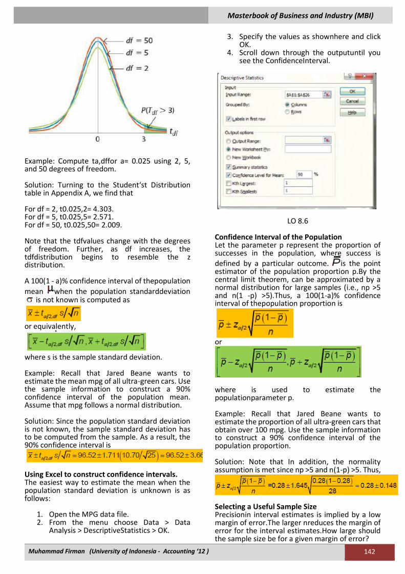
Masterbook of Business and Industry (MBI)
Muhammad Firman (University of Indonesia - Accounting ‘12 ) 142
Example: Compute ta,dffor a= 0.025 using 2, 5, and 50 degrees of freedom. Solution: Turning to the Student‘st Distribution table in Appendix A, we find that For df = 2, t0.025,2= 4.303. For df = 5, t0.025,5= 2.571. For df = 50, t0.025,50= 2.009. Note that the tdfvalues change with the degrees of freedom. Further, as df increases, the tdfdistribution begins to resemble the z distribution. A 100(1 - a)% confidence interval of thepopulation
mean when the population standarddeviation is not known is computed as
or equivalently,
where s is the sample standard deviation. Example: Recall that Jared Beane wants to estimate the mean mpg of all ultra-green cars. Use the sample information to construct a 90% confidence interval of the population mean. Assume that mpg follows a normal distribution. Solution: Since the population standard deviation is not known, the sample standard deviation has to be computed from the sample. As a result, the 90% confidence interval is
Using Excel to construct confidence intervals. The easiest way to estimate the mean when the population standard deviation is unknown is as follows:
1. Open the MPG data file. 2. From the menu choose Data > Data
Analysis > DescriptiveStatistics > OK.
3. Specify the values as shownhere and click OK.
4. Scroll down through the outputuntil you see the ConfidenceInterval.
LO 8.6 Confidence Interval of the Population Let the parameter p represent the proportion of successes in the population, where success is
defined by a particular outcome. is the point estimator of the population proportion p.By the central limit theorem, can be approximated by a normal distribution for large samples (i.e., np >5 and n(1 -p) >5).Thus, a 100(1-a)% confidence interval of thepopulation proportion is
or
where is used to estimate the populationparameter p. Example: Recall that Jared Beane wants to estimate the proportion of all ultra-green cars that obtain over 100 mpg. Use the sample information to construct a 90% confidence interval of the population proportion. Solution: Note that In addition, the normality assumption is met since np >5 and n(1-p) >5. Thus,
Selecting a Useful Sample Size Precisionin interval estimates is implied by a low margin of error.The larger nreduces the margin of error for the interval estimates.How large should the sample size be for a given margin of error?
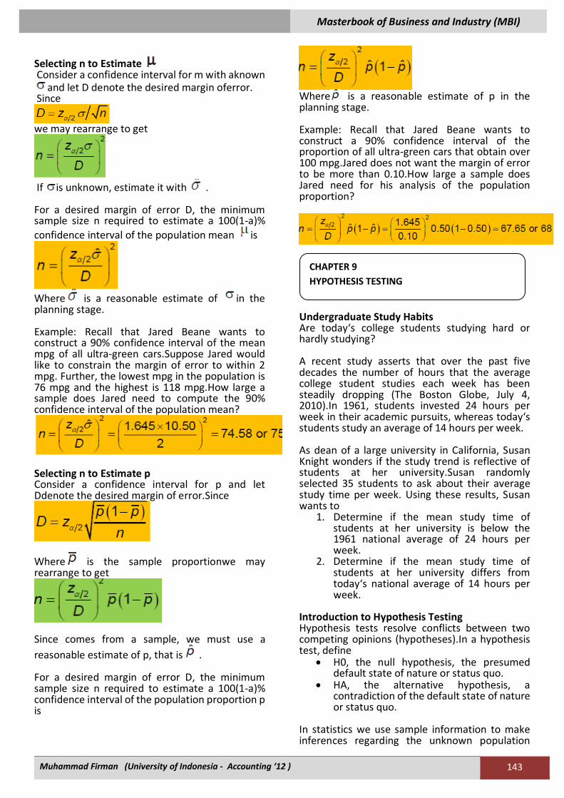
Masterbook of Business and Industry (MBI)
Muhammad Firman (University of Indonesia - Accounting ‘12 ) 143
Selecting n to Estimate Consider a confidence interval for m with aknown
and let D denote the desired margin oferror. Since
we may rearrange to get
If is unknown, estimate it with . For a desired margin of error D, the minimum sample size n required to estimate a 100(1-a)%
confidence interval of the population mean is
Where is a reasonable estimate of in the planning stage. Example: Recall that Jared Beane wants to construct a 90% confidence interval of the mean mpg of all ultra-green cars.Suppose Jared would like to constrain the margin of error to within 2 mpg. Further, the lowest mpg in the population is 76 mpg and the highest is 118 mpg.How large a sample does Jared need to compute the 90% confidence interval of the population mean?
Selecting n to Estimate p Consider a confidence interval for p and let Ddenote the desired margin of error.Since
Where is the sample proportionwe may rearrange to get
Since comes from a sample, we must use a
reasonable estimate of p, that is . For a desired margin of error D, the minimum sample size n required to estimate a 100(1-a)% confidence interval of the population proportion p is
Where is a reasonable estimate of p in the planning stage. Example: Recall that Jared Beane wants to construct a 90% confidence interval of the proportion of all ultra-green cars that obtain over 100 mpg.Jared does not want the margin of error to be more than 0.10.How large a sample does Jared need for his analysis of the population proportion?
Undergraduate Study Habits Are today‘s college students studying hard or hardly studying? A recent study asserts that over the past five decades the number of hours that the average college student studies each week has been steadily dropping (The Boston Globe, July 4, 2010).In 1961, students invested 24 hours per week in their academic pursuits, whereas today‘s students study an average of 14 hours per week. As dean of a large university in California, Susan Knight wonders if the study trend is reflective of students at her university.Susan randomly selected 35 students to ask about their average study time per week. Using these results, Susan wants to
1. Determine if the mean study time of students at her university is below the 1961 national average of 24 hours per week.
2. Determine if the mean study time of students at her university differs from today‘s national average of 14 hours per week.
Introduction to Hypothesis Testing Hypothesis tests resolve conflicts between two competing opinions (hypotheses).In a hypothesis test, define
• H0, the null hypothesis, the presumed default state of nature or status quo.
• HA, the alternative hypothesis, a contradiction of the default state of nature or status quo.
In statistics we use sample information to make inferences regarding the unknown population
CHAPTER 9
HYPOTHESIS TESTING
Masterbook of Business and Industry (MBI)
Muhammad Firman (University of Indonesia - Accounting ‘12 ) 144
parameters of interest.We conduct hypothesis tests to determine if sample evidence contradicts H0.On the basis of sample information, we either : ―Reject the null hypothesis‖, Sample evidence isinconsistent with H0. ―Do not reject the null hypothesis, Sample evidence is not inconsistent with H0, We do not have enough evidence to accept‖ H0. Defining the Null Hypothesis and Alternative Hypothesis General guidelines:
• Null hypothesis, H0, states the status quo. • Alternative hypothesis, HA, states
whatever we wish to establish (i.e., contests the status quo).
Use the following signs in hypothesis tess
Note that H0always contains the equality.‖ One-Tailed versus Two-Tailed Hypothesis Tests Two-Tailed Test Reject H0on either side of the hypothesized value of the population parameter. For example:
The ≠‖ symbol in HAindicates that both tail areas of the distribution will be used to make the decision regarding the rejection of H0. One-Tailed Test Reject H0only on one side of the hypothesized value of the population parameter. For example:
Note that the inequality in HAdetermines which tail area will be used to make the decision regarding the rejection of H0. Three Steps to Formulate Hypotheses 1.Identify the relevant population parameter of interest (e.g., or p). 2.Determine whether it is a one-or a two-tailed test
3.Include some form of the equality sign in H0and use HAto establish a claim. Example: A trade group predicts that back-to-school spending will average $606.40 per family this year. A different economic model is needed if the prediction is wrong.
• Parameter of interest is msince we are interested in the average back-to-school spending.
• Since we want to determine if the population mean differs from $606.4 (i.e, ≠), it is a two-tail test.
Example: A television research analyst wishes to test a claim that more than 50% of the households will tune in for a TV episode. Specify the null and the alternative hypotheses to test the claim.
• Parameter of interest is psince we are interested in the proportion of households.
• Since the analyst wants to determine whether p> 0.50,it is a one-tail test.
Type I and Type II Errors Type I Error: Committedwhen we reject H0when H0is actually true.Occurs with probability a. ais chosen apriori. Type II Error: Committed when we do not reject H0and H0is actually false.Occurs with probability β. Power of the test = 1-β For a given sample size n, a decrease in αwill increase βand vice versa.Both αand βdecrease as n increases. This table illustrates the decisions that may be made when hypothesis testing: Decision Null
Hypothesis is true
Null hpothesis is false
Reject the null hpothesis
Type I error Correct decision
Don’t reject the null hpothesis
Correct decision
Type II error
Correct Decisions:
• Reject H0when H0is false. • Do not reject H0when H0is true.
Incorrect Decisions:
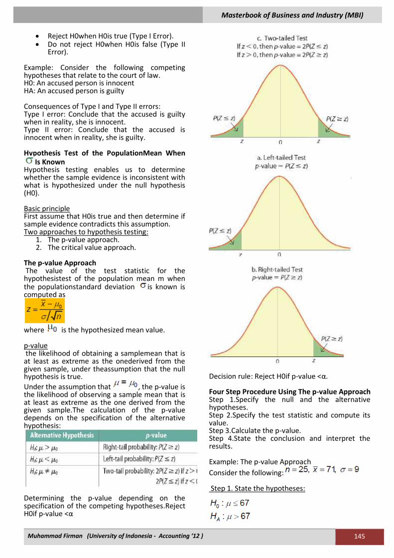
Masterbook of Business and Industry (MBI)
Muhammad Firman (University of Indonesia - Accounting ‘12 ) 145
• Reject H0when H0is true (Type I Error). • Do not reject H0when H0is false (Type II
Error). Example: Consider the following competing hypotheses that relate to the court of law. H0: An accused person is innocent HA: An accused person is guilty Consequences of Type I and Type II errors: Type I error: Conclude that the accused is guilty when in reality, she is innocent. Type II error: Conclude that the accused is innocent when in reality, she is guilty. Hypothesis Test of the PopulationMean When
Is Known Hypothesis testing enables us to determine whether the sample evidence is inconsistent with what is hypothesized under the null hypothesis (H0). Basic principle First assume that H0is true and then determine if sample evidence contradicts this assumption. Two approaches to hypothesis testing:
1. The p-value approach. 2. The critical value approach.
The p-value Approach The value of the test statistic for the hypothesistest of the population mean m when the populationstandard deviation is known is computed as
where is the hypothesized mean value. p-value the likelihood of obtaining a samplemean that is at least as extreme as the onederived from the given sample, under theassumption that the null hypothesis is true.
Under the assumption that , the p-value is the likelihood of observing a sample mean that is at least as extreme as the one derived from the given sample.The calculation of the p-value depends on the specification of the alternative hypothesis:
Determining the p-value depending on the specification of the competing hypotheses.Reject H0if p-value <α
Decision rule: Reject H0if p-value <α. Four Step Procedure Using The p-value Approach Step 1.Specify the null and the alternative hypotheses. Step 2.Specify the test statistic and compute its value. Step 3.Calculate the p-value. Step 4.State the conclusion and interpret the results. Example: The p-value Approach
Consider the following: Step 1. State the hypotheses:
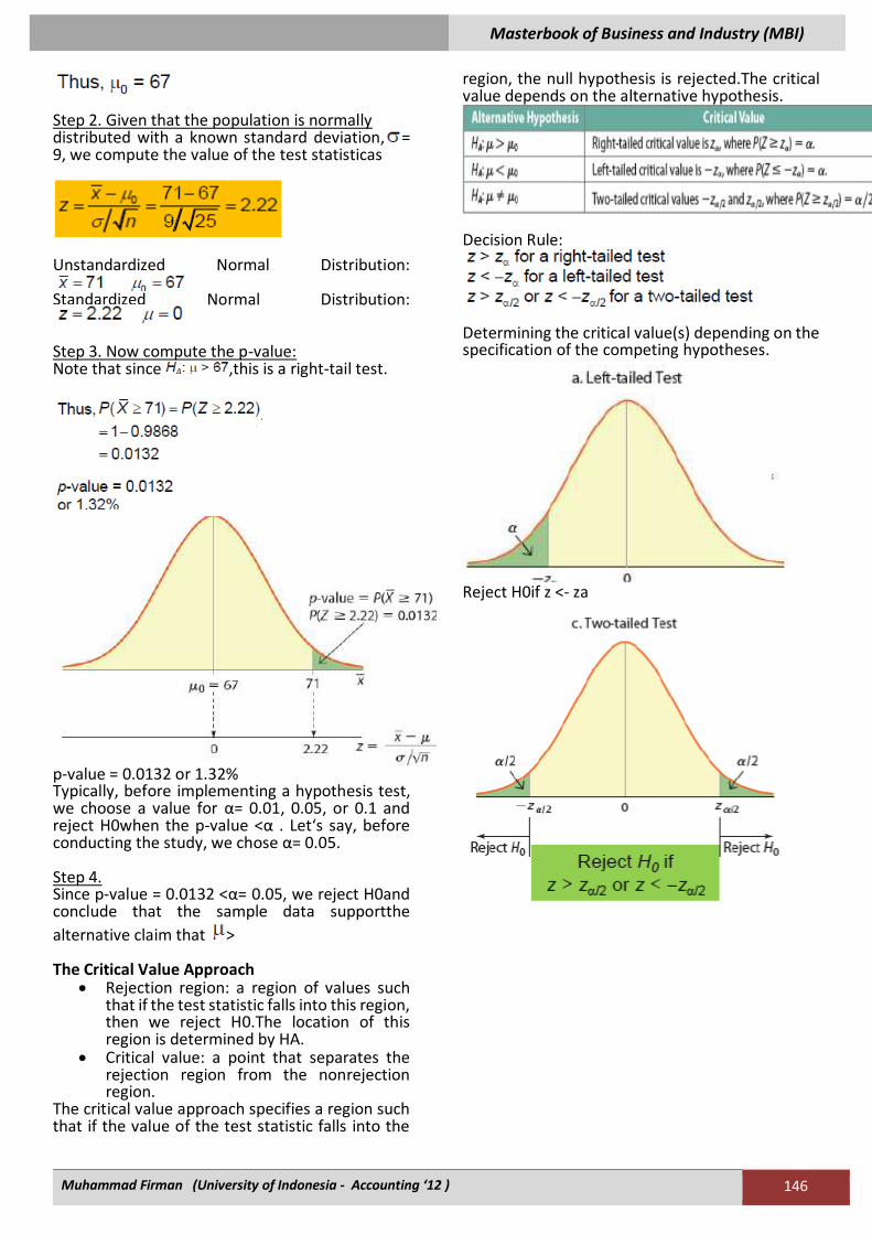
Masterbook of Business and Industry (MBI)
Muhammad Firman (University of Indonesia - Accounting ‘12 ) 146
Step 2. Given that the population is normally distributed with a known standard deviation, = 9, we compute the value of the test statisticas
Unstandardized Normal Distribution:
Standardized Normal Distribution:
Step 3. Now compute the p-value: Note that since ,this is a right-tail test.
p-value = 0.0132 or 1.32% Typically, before implementing a hypothesis test, we choose a value for α= 0.01, 0.05, or 0.1 and reject H0when the p-value <α . Let‘s say, before conducting the study, we chose α= 0.05. Step 4. Since p-value = 0.0132 <α= 0.05, we reject H0and conclude that the sample data supportthe
alternative claim that > The Critical Value Approach
• Rejection region: a region of values such that if the test statistic falls into this region, then we reject H0.The location of this region is determined by HA.
• Critical value: a point that separates the rejection region from the nonrejection region.
The critical value approach specifies a region such that if the value of the test statistic falls into the
region, the null hypothesis is rejected.The critical value depends on the alternative hypothesis.
Decision Rule:
Determining the critical value(s) depending on the specification of the competing hypotheses.
Reject H0if z <- za
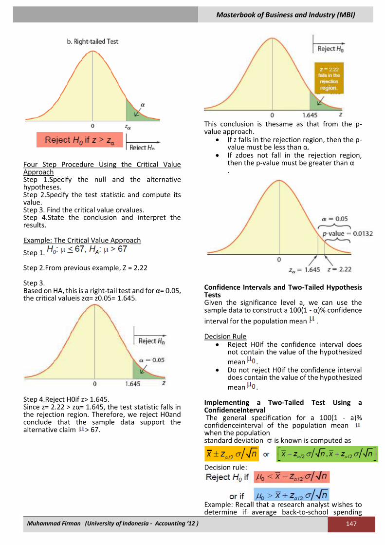
Masterbook of Business and Industry (MBI)
Muhammad Firman (University of Indonesia - Accounting ‘12 ) 147
Four Step Procedure Using the Critical Value Approach Step 1.Specify the null and the alternative hypotheses. Step 2.Specify the test statistic and compute its value. Step 3. Find the critical value orvalues. Step 4.State the conclusion and interpret the results. Example: The Critical Value Approach
Step 1. Step 2.From previous example, Z = 2.22 Step 3. Based on HA, this is a right-tail test and for α= 0.05, the critical valueis zα= z0.05= 1.645.
Step 4.Reject H0if z> 1.645. Since z= 2.22 > zα= 1.645, the test statistic falls in the rejection region. Therefore, we reject H0and conclude that the sample data support the alternative claim > 67.
This conclusion is thesame as that from the p-value approach.
• If z falls in the rejection region, then the p-value must be less than α.
• If zdoes not fall in the rejection region, then the p-value must be greater than α .
Confidence Intervals and Two-Tailed Hypothesis Tests Given the significance level a, we can use the sample data to construct a 100(1 - α)% confidence
interval for the population mean . Decision Rule
• Reject H0if the confidence interval does not contain the value of the hypothesized
mean . • Do not reject H0if the confidence interval
does contain the value of the hypothesized
mean . Implementing a Two-Tailed Test Using a ConfidenceInterval The general specification for a 100(1 - a)% confidenceinterval of the population mean when the population standard deviation is known is computed as
Decision rule:
Example: Recall that a research analyst wishes to determine if average back-to-school spending
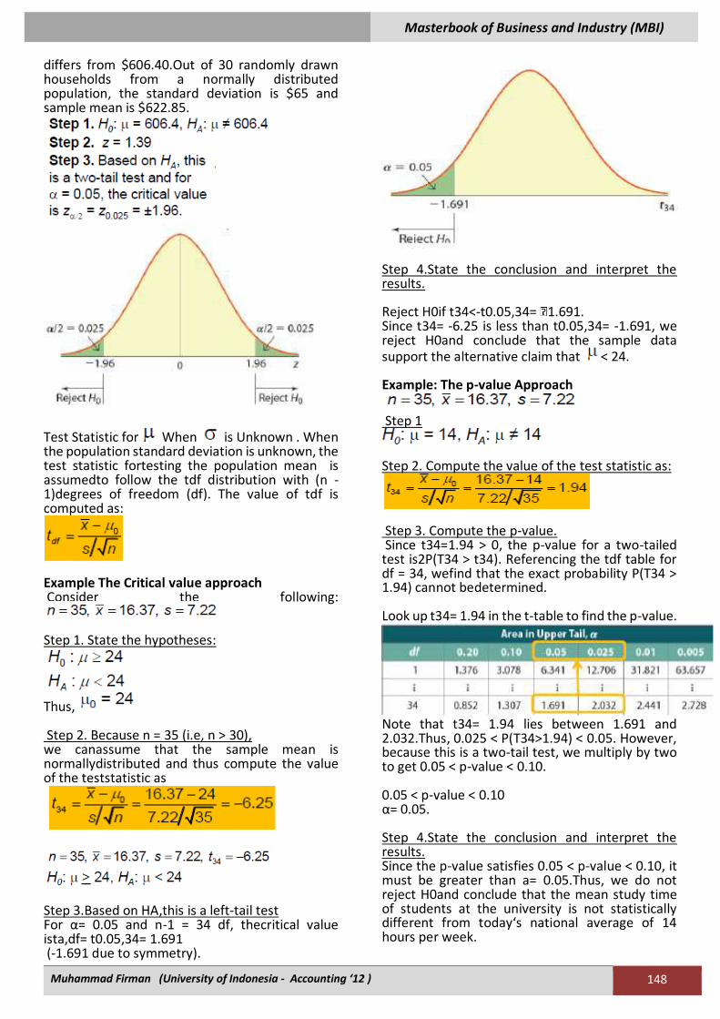
Masterbook of Business and Industry (MBI)
Muhammad Firman (University of Indonesia - Accounting ‘12 ) 148
differs from $606.40.Out of 30 randomly drawn households from a normally distributed population, the standard deviation is $65 and sample mean is $622.85.
Test Statistic for When is Unknown . When the population standard deviation is unknown, the test statistic fortesting the population mean is assumedto follow the tdf distribution with (n - 1)degrees of freedom (df). The value of tdf is computed as:
Example The Critical value approach Consider the following:
Step 1. State the hypotheses:
Thus, Step 2. Because n = 35 (i.e, n > 30), we canassume that the sample mean is normallydistributed and thus compute the value of the teststatistic as
Step 3.Based on HA,this is a left-tail test For α= 0.05 and n-1 = 34 df, thecritical value ista,df= t0.05,34= 1.691 (-1.691 due to symmetry).
Step 4.State the conclusion and interpret the results. Reject H0if t34<-t0.05,34= 1.691. Since t34= -6.25 is less than t0.05,34= -1.691, we reject H0and conclude that the sample data support the alternative claim that < 24. Example: The p-value Approach
Step 1
Step 2. Compute the value of the test statistic as:
Step 3. Compute the p-value. Since t34=1.94 > 0, the p-value for a two-tailed test is2P(T34 > t34). Referencing the tdf table for df = 34, wefind that the exact probability P(T34 > 1.94) cannot bedetermined. Look up t34= 1.94 in the t-table to find the p-value.
Note that t34= 1.94 lies between 1.691 and 2.032.Thus, 0.025 < P(T34>1.94) < 0.05. However, because this is a two-tail test, we multiply by two to get 0.05 < p-value < 0.10. 0.05 < p-value < 0.10 α= 0.05. Step 4.State the conclusion and interpret the results. Since the p-value satisfies 0.05 < p-value < 0.10, it must be greater than a= 0.05.Thus, we do not reject H0and conclude that the mean study time of students at the university is not statistically different from today‘s national average of 14 hours per week.
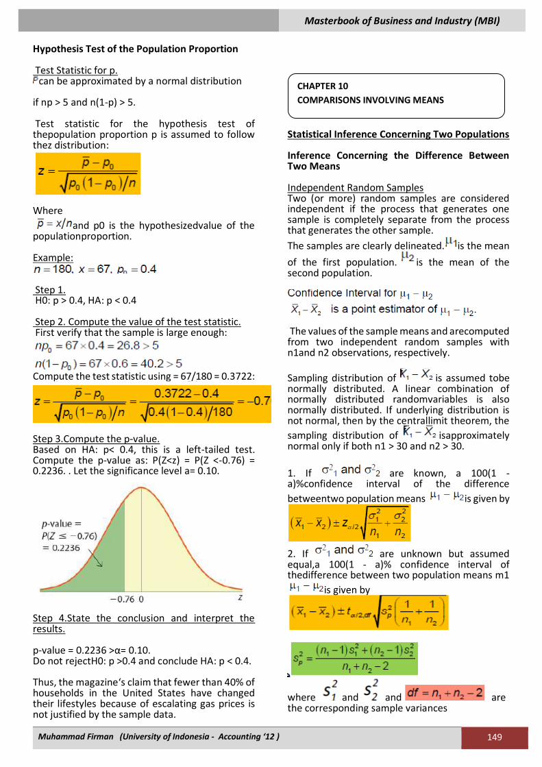
Masterbook of Business and Industry (MBI)
Muhammad Firman (University of Indonesia - Accounting ‘12 ) 149
Hypothesis Test of the Population Proportion Test Statistic for p.
can be approximated by a normal distribution if np > 5 and n(1-p) > 5. Test statistic for the hypothesis test of thepopulation proportion p is assumed to follow thez distribution:
Where
and p0 is the hypothesizedvalue of the populationproportion. Example:
Step 1. H0: p > 0.4, HA: p < 0.4 Step 2. Compute the value of the test statistic. First verify that the sample is large enough:
Compute the test statistic using = 67/180 = 0.3722:
Step 3.Compute the p-value. Based on HA: p< 0.4, this is a left-tailed test. Compute the p-value as: P(Z<z) = P(Z <-0.76) = 0.2236. . Let the significance level a= 0.10.
Step 4.State the conclusion and interpret the results. p-value = 0.2236 >α= 0.10. Do not rejectH0: p >0.4 and conclude HA: p < 0.4. Thus, the magazine‘s claim that fewer than 40% of households in the United States have changed their lifestyles because of escalating gas prices is not justified by the sample data.
Statistical Inference Concerning Two Populations Inference Concerning the Difference Between Two Means Independent Random Samples Two (or more) random samples are considered independent if the process that generates one sample is completely separate from the process that generates the other sample.
The samples are clearly delineated. is the mean
of the first population. is the mean of the second population.
The values of the sample means and arecomputed from two independent random samples with n1and n2 observations, respectively.
Sampling distribution of is assumed tobe normally distributed. A linear combination of normally distributed randomvariables is also normally distributed. If underlying distribution is not normal, then by the centrallimit theorem, the
sampling distribution of isapproximately normal only if both n1 > 30 and n2 > 30.
1. If are known, a 100(1 - a)%confidence interval of the difference
betweentwo population means is given by
2. If are unknown but assumed equal,a 100(1 - a)% confidence interval of thedifference between two population means m1
is given by
where and and are the corresponding sample variances
CHAPTER 10
COMPARISONS INVOLVING MEANS
Masterbook of Business and Industry (MBI)
Muhammad Firman (University of Indonesia - Accounting ‘12 ) 150
3. If are unknown but cannot be assumed to be equal, a 100(1 - a)% confidenceinterval of the difference between two
populationmeans is given by
Hypothesis Test for When conducting hypothesis tests concerning
, the competing hypotheses will take one of the following forms:
where d0is the hypothesized difference betweenm1and m2.10.1 Inference Concerning the
Difference Between Two Means
Test Statistic for Testing when thesampling distribution for is normal.
1. If 2 are known, then the test statistic is assumed to follow the z distribution and its valueis calculated as
2. If are unknown but assumed equal,then the test statistic is assumed to follow thetdf distribution and its value is calculated as
Where
And
3. If are unknown and cannot be assumedequal, then thetest statistic is assumed tofollow the tdf distribution andits value is calculated as:
Where
is rounded down to the nearest integer. Inference Concerning Mean Differences Matched-Pairs Sampling Parameter of interest is the mean difference Dwhere D = X1-X2, and the random variables X1and X2are matched in a pair.Both X1and X2are normally distributed or n>30.For example, assess the benefits of a new medical treatment by evaluating the same patients before(X1) and after (X2) the treatment.
Confidence Interval for A 100(1 - a)% confidence interval of the
meandifference is given by
where and are the mean and thestandard deviation, respectively, of the nsample differences, and df = n - 1.
Hypothesis Test for When conducting hypothesis tests concerning mD, the competing hypotheses will take one of the following forms:
where d0typically is equal to 0.
Test Statistic for Hypothesis Tests About
The test statistic for hypothesis tests about is assumed to follow the tdf distribution withdf = n - 1, and its value is
where and are the mean and standarddeviation, respectively, of the n sampledifferences, and d0 is a given hypothesizedmean difference. Features of the F distribution Inferences about the ratio of two populationvariances are based on the ratio of thecorresponding sample variances . These inferences are based on a new distribution: the F distribution.. iIt is common to use the notation F(df1,df2) whenreferring to the F distribution.The distribution of the ratio of the sample variances is the F(df1,df2)distribution.Since the F(df1,df2)distribution is a family of distributions, each one is defined by two degrees of freedom parameters, one for the numerator and one for
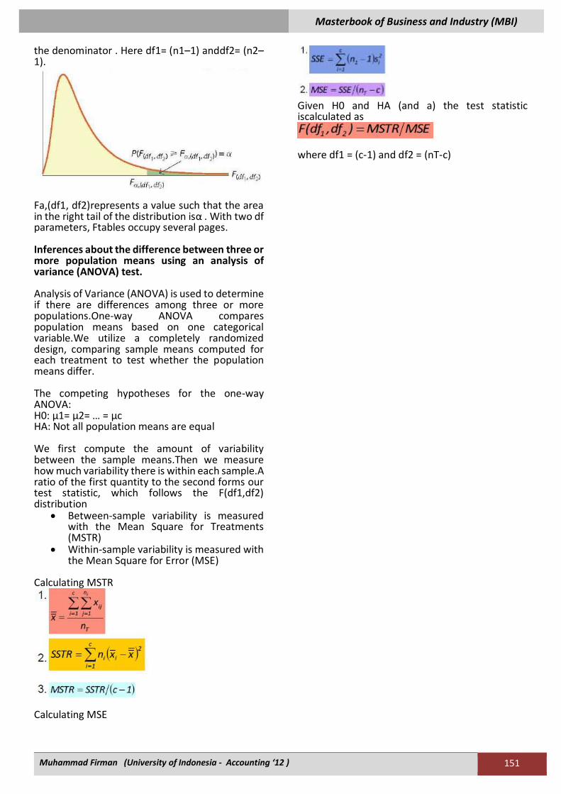
Masterbook of Business and Industry (MBI)
Muhammad Firman (University of Indonesia - Accounting ‘12 ) 151
the denominator . Here df1= (n1–1) anddf2= (n2–1).
Fa,(df1, df2)represents a value such that the area in the right tail of the distribution isα . With two df parameters, Ftables occupy several pages. Inferences about the difference between three or more population means using an analysis of variance (ANOVA) test. Analysis of Variance (ANOVA) is used to determine if there are differences among three or more populations.One-way ANOVA compares population means based on one categorical variable.We utilize a completely randomized design, comparing sample means computed for each treatment to test whether the population means differ. The competing hypotheses for the one-way ANOVA: H0: μ1= μ2= … = μc HA: Not all population means are equal We first compute the amount of variability between the sample means.Then we measure how much variability there is within each sample.A ratio of the first quantity to the second forms our test statistic, which follows the F(df1,df2) distribution
• Between-sample variability is measured with the Mean Square for Treatments (MSTR)
• Within-sample variability is measured with the Mean Square for Error (MSE)
Calculating MSTR
Calculating MSE
Given H0 and HA (and a) the test statistic iscalculated as
where df1 = (c-1) and df2 = (nT-c)