Statistics to Measure Offshoring and its Impact

by

Robert C. Feenstra

University of California, Davis, and NBER

October 1, 2016

Abstract

We identify “first generation” statistics to measure offshoring as the share of imported

intermediate inputs in costs, along with O*NET data to measure the tradability of tasks. These

data were used to measure the shifts in relative labor demand and relative wages due to

offshoring. A limitation of these statistics is that they cannot be used to measure the impact on

real wages, and for that purpose, we need price-based measures of offshoring. More recently,

“second generation” statistics have arisen from global input-output tables. These measures

include the foreign value-added in exports, or its counterpart, the domestic value-added in

exports. We illustrate the foreign value-added component in the surge of Chinese exports

following its WTO entry in 2001. We argue that such second-generation statistics should also be

supplemented by price-based measure of offshoring, and we propose one simple measure that

extends the effective rate of protection on imports to apply to exported goods.

Prepared for the Fourth IMF Statistical forum, “Lifting the Small Boats: Statistics for Inclusive Growth,” November 17-18, Washington, D.C.

1

1. Introduction

From the early research on offshoring, a primary motivation was to explain the inequality

in the earnings of labor. Evidence from the United States and other countries showed that during

the 1980s the relative wages shifted towards more-skilled workers, so that a “wage gap”

developed between those with higher and lower skills. 1 To explain that gap, Feenstra and

Hanson (1996, 1997) developed a model that allows for a continuum of imported intermediate

within each industry, which are sourced from the lowest-cost country. The model predicted that

offshoring would lead to an increase in the relative demand for high-skilled labor in both the

country initiating the offshoring and in the country receiving these tasks. It follows that both

relative wage and the relative employment of skilled workers would increase in both countries,

as occurred during the 1980s. The statistic used by Feenstra and Hanson (1999) to measure

offshoring was the cost share of imported intermediate inputs in each industry.

The story for the 1990s and later is quite different. There has continued to be an increase

in the relative wage of skilled workers in U.S. manufacturing, but the relative employment of

these workers has sometimes fallen. That finding is strongly suggestive of the offshoring of

service activities, whereby the more routine service activities are sent overseas. This new form of

offshoring can be explained by Grossman and Rossi-Hansberg (2008). Their model allows for

the offshoring the tasks performed by low-skilled labor, but allows for the offshoring of tasks

that use high-skilled labor, like service tasks, as is needed to explain the more recent empirical

observations for the U.S. In the associated empirical work, O*NET data are typically used to

measure the tradability of tasks which, in addition to the imported input share, becomes another

“first generation” statistic used to measure the impact of offshoring.

1 See Bhagwati and Kosters (1994), Collins (1998), Feenstra (1998, 2000), Feenstra and Hanson (2003), Freeman (1995), Johnson and Stafford (1999), Katz and Autor (1999), Richardson (1995), and Wood (1995).

2

The share of intermediate inputs in costs can be constructed with publically-available

data only by using the so-called proportionality assumption, whereby an input used in an

industry has the same ratio of imports to domestically-sourced value as does the economy as a

whole. That assumption has been criticized (e.g. Housman et al., 2011), and can be overcome by

having either firm-level values of imported inputs, or price-based measures of imported input

use. These improved statistics are particularly important when evaluating whether offshoring

leads to real losses for low-skilled labor, beyond just changes in the relative wage. In Feenstra

and Hanson (1996), the possibility of real losses depends on whether the efficiency gains from

offshoring dominate the shift in relative wages away from that factor. So to evaluate the real

gains and losses, we need a good estimate of the efficiency gains from offshoring, as the price

measures help to provide.

In a world with globalized production, the share of inputs that are imported becomes

especially difficult to measure when goods cross border multiple times. To give an example, a

U.S import from China might contain U.S. value-added. This concern has led to “second

generation” measures of offshoring developed from global input-output tables. Measures such as

the foreign value-added in exports (Hummels et al., 2001; Johnson and Noguera, 2012, 2016;

Koopmans et al., 2014; Los et al., 2016) have been proposed to indicate the extent to which

countries are tied into global supply chains. We review these measures and give an application to

the “China shock”, i.e. to the dramatic rise in Chinese exports following its entry to the World

Trade Organization in 2001. We measure the extent to which different countries have shared in

this export increase through their value-added in China. We further use the global input-output

framework to develop a new price-based measure of global offshoring, which extends the

effective rate of protection on imports to apply to exported goods.

3

In section 2 we review the data on the wage and employment of nonproduction relative to

production workers in the United States, which was the starting point for the early literature on

offshoring. The models developed to explain those trends are presented in sections 3 and 4, along

with the tests of those models using the cost share of intermediate inputs and O*NET data as

offshoring statistics. Limitations of those statistics are discussed in section 5. More recent

literature uses global input-output tables to measure offshoring and has its own set of limitations,

as discussed in sections 6 and 7. The price-based measure of global offshoring is presented in

section 8, where we argue that China’s own reduction in its tariffs on imported inputs can

partially explain its export surge (see also Amiti et al., 2016). Section 9 concludes.

2. Offshoring and Wage Inequality

We begin by examining the pattern of wages over time in U.S. manufacturing, which

motivated the early research on offshoring. In Figures 1 and 2 we show the wage and

employment of “nonproduction” relative to “production” workers in U.S. manufacturing.

Nonproduction workers tend to require more education, and so we will treat these workers as

skilled, while production workers are treated as less-skilled, though these categories are

admittedly highly imperfect measures of skill.

In Figure 1, we see that the earnings of nonproduction relative to production workers

moved erratically from the late 1950s to the late 1960s, and from that point until the early 1980s,

relative wages were on a downward trend. It is generally accepted that the relative wage fell

during this period because of an increase in the supply of college graduates, skilled workers who

moved into nonproduction jobs. Starting in the early 1980s, however, this trend reversed itself

and the relative wage of nonproduction workers increased steadily to 2000, with a decline to

2005 and a further increase thereafter.

4

Figure 1: Relative Wage of Nonproduction/Production Workers, U.S. Manufacturing, 1958-2014

Figure 2: Relative Employment of Nonproduction/Production Workers, U.S. Manufacturing, 1958-2014

Source: NBER productivity database, updated after 1996 from Bureau of the Census.

5

Turning to Figure 2, we see that there was a steady increase in the ratio of nonproduction

to production workers through the end of the 1980s, but then a fall in the 1990s, with an erratic

recovery since 2000. The increase in the relative supply of workers through the 1970s can

account for the reduction in the relative wage of nonproduction workers that decade, as shown in

Figure 1, but is at odds with the increase in the relative nonproduction wage during the 1980s.

The rising relative wage should have led to a shift in employment away from skilled workers,

along a demand curve, but it did not. Thus, the only explanation consistent with these facts is that

there was an outward shift in the demand for more-skilled workers during the 1980s, leading to

an increase in their relative employment and wages, as shown in Figure 3.

What factors can lead to an outward shift in the relative demand for skilled labor? Such a

shift can arise from the use of computers and other high-tech equipment, or skill-biased

technological change. Researchers such as Berman, Bound and Griliches (1994) argued that such

technological change was the dominant explanation for the rising relative wage of skilled labor

in the United States, and other countries. Their findings for the United States were reinforced by

the work of Berman, Bound and Machin (1998) who looked at cross-country data. They found

that the same shift towards skilled workers in the U.S. also occurred abroad. That finding

appeared to rule out the Heckscher-Ohlin (HO) model as an explanation, because in that model

we expect wages to move in opposite directions between countries when comparing autarky to

free trade, as factor price equalization occurs. Instead, the evidence was that wages moved in the

same direction across countries – with an increase in the relative wage of skilled workers. 2

2 The same decline in the relative wages of blue-collar workers during the 1980s and into the 1990s was found for Australia, Canada, Japan, Sweden, and the United Kingdom (Anderton and Brenton 1999; Freeman and Katz 1994; Katz and Autor 1999; Görg, Hijzen, and Hine 2003, 2005), for Hong Kong and Mexico (Cragg and Epelbaum 1996; Hanson and Harrison 1999; Hsieh and Woo 2005; Robertson 2004), and for Denmark (Hummels et al. 2014) over 1995–2006. More recent evidence for the United States is provided by Voigtländer (2014).

6

Figure 3: Relative Wage and Employment of Nonproduction/Production Workers in U.S. Manufacturing, 1979-1990

1989

1990

1979

1980 1981

1982

19861983

1985

19841987

1988

1.50

1.55

1.60

1.65

0.2 0.25 0.3 0.35 0.4 0.45 0.5 0.55 0.6

Nonproduction/Production Employment

No

np

rod

uct

ion

/Pro

du

ctio

n W

age

Source: NBER productivity database; see Figures 1 and 2.

But this early rejection of international trade as an explanation for rising wage inequality

was really just a rejection of the simple HO model. There are now several models of offshoring

that can be used to predict the wages movements for the 1980s as shown in Figure 3, and also

wage movements in later decades, as we review below.

3. A Model of Offshoring

To determine the extent to which international trade can explain the shift in demand

towards skilled labor in the United States, and which occurred in other countries, Feenstra and

Hanson (1996, 1997) present a model of an industry in which there are many intermediate inputs,

denoted by the index z[0,1], involved in the manufacture of a good. Rather than listing these

7

inputs in their temporal order, we will instead list them in increasing order of high/low-skilled

labor where, for example, the least skill-intensive input is assembly and the most skill-intensive

input is R&D. We let aH(z) and aL(z) denote the high-skilled and low-skilled labor, respectively,

needed to produce one unit of the good in question. We order the activities z so that

aH(z)/aL(z) is non-decreasing in z.

In general, firms doing the assembly will wish to source the inputs from the minimum-

cost location. To determine this, we assume that the relative wage of skilled labor at home,

H Lw / w , is lower at home than that abroad, H Lw / w < * *H Lw / w . This assumption is realistic if

the home country is skilled-labor abundant, like the United States: despite the increase in the

relative wage of skilled labor in the United States during the past several decades, it is still much

lower than that in Mexico.

In equilibrium, countries will specialize in different portions along the continuum of

intermediate inputs. Under our assumption that the relative wage of skilled labor is higher

abroad, and that goods are arranged in increasing order of their skill intensity, then the ratio of

the home to foreign unit-costs is downward sloping, as shown by the schedule c/c* in Figure 4.

Foreign production – or offshoring – occurs where the relative costs at home are greater than

unity, in the range [0,z'), whereas home production occurs where the relative costs at home are

less than unity, in the range (z',1].

Suppose now that the home firm wishes to offshore more activities. The reason for this

could be a capital flow from the home to foreign country, reducing the rental abroad and

increasing it at home; or alternatively, it could arise from neutral technological progress abroad,

but exceeding such progress at home. In both cases, the relative costs of production at home

8

Figure 4

increase, which is an upward shift in the relative cost schedule, as shown in Figure 5. As a result,

the borderline between the activities performed at home and abroad therefore shifts from the

point z' to the point z", with z" > z'.

What is the impact of this increase in offshoring on the relative demand for skilled labor

at home and abroad? Notice that the activities no longer performed at home (those in-between z'

and z") are less skill-intensive than the activities still done there (those to the right of z"). This

means that the range of activities now done at home are more skilled-labor intensive, on average,

than the set of activities formerly done at home. For this reason, the relative demand for skilled

labor at home increases, as occurred in the United States during the 1980s. That increase in

demand will also increase the relative wage for skilled labor, as shown in Figure 6 (where we use

a fixed relative supply of high/low-skilled labor, but it could be upward sloping instead).

0 z' 1 z

c/c*

c/c*

A

9

Figure 5

Figure 6

D(z")

D(z')

H/L

wH/wL

B

0 z' z" 1 z

c/c*

1

c/c*

A

c'/c*'

10

What about in the foreign country? The activities that are newly sent offshore (those in-

between z' and z") are more skill-intensive than the activities that were initially done in the

foreign country (those to the left of z'). That means that the range of activities now done abroad

is also more skilled-labor intensive, on average, than the set of activities formerly done there. For

this reason, the relative demand for high-skilled labor in the foreign country also increases, just

as shown in Figure 6. With this increase in the relative demand for high-skilled labor, the relative

wage of skilled labor also increases in the foreign country. This is a realistic description of the

wage movements in the United States and many other countries during the 1980s.3

In contrast to this result, it is difficult to generate the same direction of movements in

relative wages across countries from the HO model, as we have found in this offshoring model.

Of course, this explanation does not prove that offshoring was the source of the wage changes,

since skill-biased technological change is equally well an explanation. So determining which of

these explanations accounts for the changes observed during the 1980s is an empirical question.

We review the literature on this question and then discuss the wage movements for the U.S. in

the 1990s and 2000s.

4. Testing the Model of Offshoring

Evidence from the 1980s

Feenstra and Hanson (1999) measure offshoring in each industry by the share of imported

intermediate inputs in costs. This measure is constructed from input-output tables using the so-

called “proportionality” assumption, e.g. that steel imported into the automobile industry uses the

same ratio of imports to domestically-sourced inputs as does the economy as a whole. This

measure of offshoring can be constructed using either a broad definition, which includes all

3 See note 2.

11

imported inputs, or a narrow definition, which focuses on imported inputs within the same 2-

digit industry (e.g. the automobile industry importing auto parts). High-technology equipment is

also measured in two ways: either as a fraction of the total capital equipment installed in each

industry; or as a fraction of new investment in capital that is devoted to computers and other

high-tech devices.

An increase in offshoring as illustrated in Figure 6 can be treated as an (exogenous) shift

to labor demand, and its impact can be measured by estimating the associated labor demand

system.4 Here we simply describe the results from this estimation. In Table 1, the results from

the broader measure of offshoring are reported, including imported inputs from other industries,

for the 1980s. Using the first measure of high-tech equipment (i.e. fraction of the capital stock),

the results in the first row show that roughly 25% of the increase in the relative wage of

nonproduction workers was explained by offshoring, and about 30% of that increase was

explained by the growing use of high-tech capital. So we conclude that both offshoring and the

increased use of high-tech capital are important in explaining the actual increase in the relative

wage of skilled workers. In the second row we use the other measure of high-tech equipment (i.e.

fraction of new investment). In that case, the large spending on high-tech equipment in new

investment can explain nearly all (99%) of the increased relative wage for nonproduction

workers, leaving little room for offshoring to play much of a role (it explains only 12% of the

increase in the relative wage). These results are lopsided enough that we might be skeptical of

using new investment to measure high-tech equipment and therefore prefer the results using the

capital stocks.

4 Wright (2014) introduces an instrumental variable strategy to treat this offshoring statistic as endogenous, based on a “shift-share” analysis that interacts each industry’s initial level of offshoring to China with China’s subsequent growth in offshoring to the U.S. over all industries.

12

Table 1: Impact on the Relative Wage of Nonproduction Labor in U.S. Manufacturing, 1979-1990

Percent of Total Increase Explained by each Factor High-technology Offshoring Equipment Measurement of high-tech equipment:

As a share of the capital stock 21 – 27% 29 – 32%

As a share of capital flow (i.e. new investment) 12% 99%

Source: Robert C. Feenstra and Gordon H. Hanson, “The Impact of Outsourcing and High-Technology Capital on Wages: Estimates for the U.S., 1979-1990,” Quarterly Journal of Economics, August 1999, 114(3), 907-940.

Evidence from the 1990’s and 2000s

In Figure 7 we report the relative wage and employment of nonproduction/production

workers in U.S. manufacturing over 1990-2000. While picture for the 1980s is well-known and

launched dozens of research studies, but it is surprising that the picture for the 1990s and 2000s,

as shown in Figure 7, is not familiar. We see that from 1989-1999 (shown in red), there

continued to be an increase in the relative wage of nonproduction/production labor in U.S.

manufacturing, but in addition, there was a decrease in the relative employment of these

workers. From 2000-2005 (shown in green), there are very erratic movements in the relative

wage and relative employment, sometimes reversing the 1989-2000 movements. Then, from

2006-2011 (in purple) there is once again an increase in the relative wage and the relative

employment of high-skilled labor, as we found for the 1980s. The final two years that are plotted

(in yellow), 2013 and 2014, show an erratic fall in relative employment.

13

Figure 7: Relative Wage and Employment of Nonproduction/Production Workers in U.S. Manufacturing, 1989-2014

Source: NBER productivity database; see Figures 1 and 2.

There are two possible explanations for the pattern shown during 1989-1999, with an

increase in the relative wage but a decrease in the relative employment of skilled labor. First,

some labor economists have argued that the 1990s witnessed a changing pattern of labor

demand, benefitting those in the highest and lowest-skilled occupations, at the expense of others

in moderately skilled occupations. Autor, Katz and Kearney (2008, p. 301) attribute this once

again to technological change: “…we find that these patterns may in part be explained by a

richer version of the skill-biased technical change (SBTC) hypothesis in which information

technology complements highly educated workers engaged in abstract tasks, substitutes for

14

moderately educated workers performing routine tasks, and has less impact on low-skilled

workers performing manual tasks.” This is the job polarization explanation.

A second possibility is that the evidence over 1989-2000 shown in Figure 7 is a

“smoking gun” for service offshoring from U.S. manufacturing. To the extent that the back-

office jobs being offshored from manufacturing use the lower-paid nonproduction workers, then

the offshoring of those jobs could very well raise the average wage among nonproduction

workers, while lowering their employment.

That outcome can arise in the offshoring model of Grossman and Rossi-Hansberg (2008),

provided that we focus on the offshoring of high-skilled labor tasks rather than low-skilled tasks.

In their model, offshoring of high-skilled labor acts just like a high-skilled-labor-saving

innovation. The offshoring of high-skilled tasks, which we are thinking of as service activities,

leads to an increase in the relative wage of high-skilled labor and no change in the relative wage

of low-skilled labor.5 Furthermore, such offshoring will reduce demand for skilled labor, at given

industry outputs, as we have seen occurred in the United States during the 1990s. So an

important contribution of Grossman and Rossi-Hansberg’s model is that it gives us a robust way

to model this service offshoring in addition to the low-skilled offshoring of the 1980s. The rich

specification of offshoring costs that are built into the model allow for a wide array of outcomes,

beyond those in Feenstra and Hanson (1996, 1997).

There are several studies that document the growing importance of service offshoring for

the U.S. One study separates the impact of offshoring on production and nonproduction workers

in U.S. manufacturing for the 1990s (Sitchinava, 2008). She applies the procedure of Feenstra

and Hanson (1999), using materials offshoring and service offshoring (both measured as shares

5 See the explanation of this result in Feenstra (2010, Lecture 1) and Feenstra (2015, chapter 4).

15

of purchased inputs), as well as computer capital as shifters of labor demand. While the relative

wage of nonproduction workers continued to rise during this period, materials offshoring

explains only 7% of that increase. Service offshoring is twice as important, explaining some 15%

of the increase in the relative wage. But the increased use of computers (as a share of the capital

stock) can account for nearly the entire rise in the relative wage.

Other studies do not focus on the relative wage but on other aspects of offshoring. Amiti

and Wei (2009) find that for U.S. manufacturing, imported services grew from two-tenths of one

percent of total inputs used in 1992, to three-tenths by 2000. The fact that imported services are

so small does not prevent them from being important for productivity, however. They find that

service offshoring accounts for around 10 percent of labor productivity growth over this period,

which is quite robust across specifications, while material offshoring accounts for a smaller and

less-robust 5 percent of labor productivity growth.

What about employment? We have seen the relative employment of nonproduction

workers fell during the 1990s, in marked contrast to the 1980s. Can we attribute that fall to tasks

that require skills but are more routine, allowing them to be offshored? Amiti and Wei (2005a,b)

do not identify a significant impact of service offshoring on employment, possibly because they

work with a single aggregate of labor. But another study of white-collar employment in the

United States (Crinò, 2010), for both manufacturing and services, suggests that offshoring had an

impact. Crinò finds that service offshoring raises high-skilled employment and lowers medium

and low-skilled employment. Within each skill group, there is a differential response depending

on whether the tasks being performed are classified as “routine”, requiring “face-to-face”

communication or not, and “interaction with PCs”, which Crinò combines to obtain a tradability

index for each occupation. Service offshoring is found to penalize the tradable occupations and

16

benefit the non-tradable occupations, consistent with the theory. Crinò (2008, 2013) further

discusses the impact of service offshoring on productivity and labor demand in Western Europe.

In order to develop his “tradability” index, Crinò relied on the O*NET database which

provides information on job characteristics for 812 occupations. Ebenstein et al. (2014),

Grossman and Rossi-Hansberg (2006), Liu and Trefler (2011), Odenski (2012, 2014) and Wright

(2014) all find evidence that these O*NET characteristics make a difference for measuring the

effects of offshoring in the United States. Wright (2014) constructs an index of offshorability

from the O*NET data and test whether the extent of low-skilled (production) jobs and high-

skilled (non-production) job loss responds differently in industries that have greater

offshorability: while more low-skilled jobs are lost when the tasks done in an industry are more

routine, the opposite occurs for high-skilled jobs. That hypothesis is strongly confirmed in his

results, and in fact, the gain of high-skilled jobs more than offsets the loss in low-skilled jobs.

Adding together these two effects, he concludes that: “the aggregate effect of offshoring is

estimated to have led to a cumulative increase in aggregate employment of 2.6% over the period

2001 to 2007, a relatively minor effect” (p. 76). 6

Perhaps the most compelling argument supporting the idea that offshoring in the 1980s

was different from that in the 1990s and 2000s is provided by Basco and Mesteiri (2013). They

argue that trade liberalization in the 1980s increased trade in low-skilled goods (what they call L-

globalization), while reduction in information and communication costs in the 1990s and 2000s

increased trade in middle- and high-skilled intensive goods (what they call C-globalization).

They present a model that integrates Feenstra and Hanson (1996, 1997) with Grossman and

Rossi-Hansberg (2008), allowing for both trade in intermediate inputs and trade in tasks. The

6 Ottaviano, Peri and Wright (2013) further estimate the effects of offshoring and immigration on jobs in the United States.

17

difference between the two types of globalizations is that the reduction of trade costs applies to

different segments in the continuum of intermediate inputs/tasks. As a theoretical result, L-

globalization increased the wage of middle- and high-skilled labor relative to low-skilled labor,

but C-globalization has a quite different effect: while high-skilled labor still gains, the wage of

middle-skilled relative to low-skilled labor can fall as the demand for middle-skilled labor is

reduce due to service offshoring. This outcome accords well with the evidence on job

polarization for the United States, whereby the workers in the middle of the skill range have

suffered (Autor, Katz and Kearney, 2008). Notably, they find that the time as which wage

polarization due to C-globalization occurs is delayed when there is more L-globalization.

5. Limitations of First-Generation Offshoring Statistics

To summarize our discussion so far, by using the share of inputs that are imported to

measure offshoring, it was possible to explain the pattern of wage movements found in the

United States and other countries during the 1980s. For the 1990s and later periods, the

offshoring of service activities (using nonproduction labor) became more important, and then it

becomes necessarily to measure the offshorability of tasks using O*NET data. Are we to

conclude that these first-generation measures of offshoring and its impact are adequate enough?

Or are there important questions that are left unexplained by these statistics?

In the remainder of this paper we lean towards the second of these statements: while the

phenomenon of offshoring has been firmly integrated into both trade theory and its empirical

implementation, there are important questions not addressed by the studies we have reviewed.

The first and perhaps most important of these is the welfare impact of offshoring, especially for

low-skilled labor. Feenstra and Hanson (1996) examine this issue in theory, and conclude that

while the relative wage of low-skilled workers fall in both countries, their real wages need not

18

fall. Low-skilled workers in the home country are the most disadvantaged by the offshoring, but

nevertheless, it is possible that they gain due to lower prices of the final good. Whether or not

low-skilled labor loses depends on whether the efficiency gains from offshoring dominate the

shift in relative wages away from that factor. So to evaluate the real gains and losses, we need a

good estimate of the efficiency gains from offshoring.

A second very important issue is to improve the measures of offshoring itself. As we

have noted, the statistic introduced by Feenstra and Hanson (1999) was the share of imported

intermediate inputs in costs. That measure relies on the proportionality assumption, whereby the

ratio of imports to domestically-purchased inputs is assumed to be the same in every industry,

and so the economy-wide ratio (as obtained from a domestic input-output table) is used for every

industry. The validity of this assumption is explored by Feenstra and Jensen (2012) for the

United States and by Winkler and Milberg (2012) for Germany, and the latter authors especially

question its accuracy.

An alternative to the proportionality assumption is to use the share of inputs imported by

each firm, when such firm-level data are available. A recent example of this approach is Blaum

et al. (2016), who utilize firm-level information for France to evaluate the gains from input trade.

The availability of newly imported inputs is accounted for by using the share of spending on

those new imports, which is a sufficient statistic for gains in a CES framework, analogous to

Feenstra (1994) and Arkolakis et al. (2012). So we see that improving the measure of offshoring

by using firm-level data also turns out to give an accurate measure of the welfare gains due to

that offshoring. Still, we might not expect the firm-level import statistics to be available for all

countries in the foreseeable future.

19

Housman et al. (2011) also criticize the proportionality assumption used to construct the

imported input share, and as an alternative statistic for offshoring, propose a price-based

measure of offshoring obtained from unpublished Bureau of Economic Analysis data on

imported input prices at a detailed commodity level. These price data are used to distinguish

between domestic and imported input prices, where we expect firms to substitute towards lower-

cost foreign sources. Without such a correction to existing statistics, the growth in the import

price index will generally be overstated, with the following consequences:

As a result of this price index problem, the real growth of imported inputs has been understated. Furthermore, if input growth is understated, it follows that the growth in multifactor productivity and real value added in the manufacturing sector have been overstated. We estimate that average annual multifactor productivity growth in manufacturing was overstated by 0.1 to 0.2 percentage points and real value added growth by 0.2 to 0.5 percentage points from 1997 to 2007. Moreover, this bias may have accounted for a fifth to a half of the growth in real value added in manufacturing output excluding the computer and electronics industry. [Housman et al. (2011), p. 115]

Note that correcting the import price index to allow for the substitution of firms towards lower-

cost import sources was also recommended by Alterman (2010).

The usefulness of such price-based measure of offshoring (or the share-based measure of

new inputs as in Blaum et al., 2016) is that they facilitate measurement of the efficiency gains

from offshoring. Whether we are dealing at the firm-level, industry-level, or economy-wide

level, measuring the gains from offshoring requires knowing the prices that firms are paying for

inputs from different sources, and in particular, the price differences when they substitute across

countries. An attempt to measure this substitution as the economy-wide level for the United

States was made by Feenstra et al. (2013). They rely on import price data collected by the

International Price Program of the Bureau of Labor Statistics, and experiment with alternative

formulas for constructing the U.S. import price index as well as incorporating tariff reductions,

especially for information-technology products. Like Housman et al. (2011), whenever the

20

growth in the import price index is overstated, then the growth in import quantity will be

understated, and so overall multifactor productivity growth is also overstated. It is important to

emphasize, however, that households and firms still benefit from reductions in import prices and

the substitution towards cheaper imports, but this is a terms of trade gain rather than productivity

growth. Feenstra et al. (2013) find that such terms of trade gains (and tariff reductions) account

for nearly 0.2 percentage points, or about one-fifth of the reported 1996-2006 increase in U.S.

productivity growth, at the lower end of the estimates in Housman et al. (2011).7

6. Offshoring Statistics from Global Input-Output Tables

The studies that we have summarized in section 4, used to test the simple offshoring

model, tended to focus on the impact of offshoring in a particular country. Of course, there is

nothing to prevent that analysis being done over a larger set of countries, and a good example of

that global approach was in Chapter 5, “The Globalization of Labor”, in the World Economic

Outlook (Jaumotte and Tytell, 2007). That study allowed for trade in final goods, in intermediate

inputs, and also immigration to impact factor payments worldwide.

A limitation of these cross-country studies, however, is that they do not allow for the

global production linkages that occur when goods cross multiple borders during their production.

There are only a limited number of theoretical studies that allow for multiple countries, and even

these studies tend to have uni-directional movement of unfinished goods between countries, until

the final good is assembled and shipped worldwide.8

7 Reinsdorf and Yuskavage (2016) have recently re-examined the bias in multifactor productivity growth through not accounting for changing sourcing between domestic and imported goods, and find that one-tenth of the reported speedup in productivity over 1997-2007 can be explained by this bias. 8 For example, Costinot, Vogel and Wang (2012) model a sequential supply chain in which mistakes potentially occur at each stage in a continuum. There are many countries which differ in their probabilities of making mistakes. In equilibrium there is a matching between stages of production and countries. Baldwin and Venables (2013) call this type of sequential product chain a “snake”, and call the assembly of multiple parts at a central facility a

21

To empirically implement multi-country measures of offshoring, global input-output

tables are used, of which examples are the World Input-Output Database or WIOD (Timmer et

al., 2014, 2015), and EORA (Lenzen et al., 2012, 2013). From these databases, measures of

offshoring more complex than the simple share of imported intermediate inputs have been

proposed, and we refer to these as “second generation” statistics. Specifically, the domestic

value-added in exports and its counterpart, the foreign value-added in exports (Hummels et al.,

2001; Johnson and Noguera, 2012, 2016; Koopmans et al., 2014; Los et al., 2016), can be

constructed to indicate the extent to which countries are tied into global supply chains.9

We illustrate foreign value-added in exports, or FVAiX, by constructing it according to

the method in Foster-McGregor and Stehrer (2013). To use their illustration with three countries

and one aggregate sector, we construct the following matrix for China as country 1,

1 1*

2 1 21

3 31

1 11 12 13 1*

2 21 22 23 21

3 31 32 33 31

1 11 1* 1 12 21 1 13 31

2 21 1* 2 22 21 2

0 0 0 0

0 0 ( ) 0 0

0 0 0 0

0 0 0 0

0 0 0 0

0 0 0 0

v x

v x

v x

v l l l x

v l l l x

v l l l x

v l x v l x v l x

v l x v l x v

I A

23 31

3 31 1* 3 32 21 3 33 31

.l x

v l x v l x v l x

(1)

“spider.” They provide a partial equilibrium model that illustrates the difficulties of solving for the location of stages in this framework, and also that the assignments might be non-monotonically related to transportation costs. The difficulty of solving for the sources of import supply chosen by firms is illustrated in the work of Antràs et al. (2014), and they also provide and implement an elegant solution. 9 A different measure of the fragmentation of the production process has been developed by Antràs et al. (2012), and applied theoretically by Antràs and Chor (2013) and by Fally and Hillberry (2015).

22

In this expression, A denotes the global input-output matrix for China, detailing the domestic and

international flows between country-industries listed on the rows towards the country-industries

listed on the columns. The input-output matrix is expressed in value terms, i.e. the share of $1 in

country-industry j accounted for by the flow from country-industry i. We denote 1( ) L I A

with individual coefficient ijl in this inverse matrix. The terms iv are the ratio of value-added to

gross output for country i.10 The terms appearing on the right are country 1’s exports to the rest

of the world, 1* 12 13,x x x and country 1’s imports from country i, 1ix , for i=2,3.

Focusing on the first column of the final matrix, the term 1 11 1*v l x is the domestic value

added in the exports of country 1, or DVAiX. The sum of the remaining terms, 1 1*2,3

i ii

v l x ,

is the foreign value added in the exports of country 1, or FVAiX. The remaining columns reflect

the value added content of country 1’s imports (see Foster-McGregor and Stehrer, 2013). We

focus our attention here on China, and calculate FVAiX, because we are interested in whether

the surge in Chinese exports following its entry to the WTO in 2001 led to a corresponding rise

in the value-added of other countries as they exported to China. We expect that China might be

using other countries in Asia as part of its supply chain, as well as e.g. Australia for certain raw

material. If we also find that China is relying on the United States, then that could offset the

negative impacts that growing Chinese exports have had on U.S. wages and employment, as

found by Autor, Dorn and Hanson (2013) and Acemoglu et al. (2014).

In order to calculate FVAiX we must choose a database. WIOD includes 40 countries

plus the rest of the world, but unfortunately, these do not include the smaller countries of

Southeast Asia who might be serving as suppliers to China. So instead we turned to the EORA

10 With multiple sectors, these are the diagonal matrices with the ratio of value-added to gross output for each industry in country i. As a column vector, this can be constructed as v = 1 (I - A) ,

23

database, http://worldmrio.com/# , which has 187 countries. Because that very large number

means that some of the input-output tables are inaccurate, and because it becomes difficult to

invert the global input-output table, we aggregated across the smaller countries to arrive at 45

plus the rest of the world. That list of countries includes 11 Southeast Asian countries that do not

appear in WIOD, which are Bangladesh, Cambodia, Laos, Malaysia, Myanmar, Nepal, Pakistan,

the Philippines, Singapore, Thailand and Vietnam.11 These are in addition to 5 other Asian

countries – China, Indonesia, Japan, Republic of Korea (or South Korea), and Taiwan – that are

included in WIOD and in our aggregated EORA country list.

The result for the aggregate Chinese economy is shown in Figure 8, with the top 20

contributors to FVAiX and the Rest of the World (RoW) based on the data in 2013. In Panel A

we see that the foreign valued added in Chinese exports is about 30% in 2013, with domestic

value-added accounting for the remaining 70%. That foreign share has nearly doubled from

about 17% since China’s entry to the WTO in 2001. The countries that provide the greatest value

added in 2013 are Japan, the United States and Germany. Of course, these three countries are

also the world’s largest exporters aside from China itself. Besides them, the next countries with

the largest value added in China’s exports are all in Asia, and are South Korea, Singapore,

Thailand, Malaysia and Vietnam. These countries are followed by Mongolia, the U.K., Taiwan,

Australia, Indonesia, France, the Netherlands, Italy, Cambodia, India, the Philippines and

Belgium. So we see that Southeast Asian countries indeed show up prominently in this list of the

top 20 countries, along with Mongolia and Australia due to their proximity and raw materials,

and also a number of European nations.

11 Hong Kong and Macau are included as distinct customs regions in the calculations of FVAiX, but then are aggregated within China when reporting our results.

24

Figure 8: Foreign Value Added in Exports of China: Aggregate

A: Foreign value added by country (share)

0

0.05

0.1

0.15

0.2

0.25

0.3

Japan USA Germany South Korea Singapore Thailand Malaysia

Viet Nam Mongolia UK Taiwan Australia Indonesia France

Netherlands Italy Cambodia India Philippines Belgium RoW

B: Foreign value-added by country (value, billion US$)

0

100

200

300

400

500

600

700

Japan USA Germany South Korea Singapore Thailand Malaysia

Viet Nam Mongolia UK Taiwan Australia Indonesia France

Netherlands Italy Cambodia India Philippines Belgium RoW

Notes: The foreign value added in China’s exports is computed as illustrated by in the top-left term in equation (1), as explained in the main text. The calculation is based on the data from the EORA global input-output table (aggregated to 45 countries), showing the top 20 contributors and the Rest of the World (RoW) based on the data in 2013.

25

In panel B we show information but now in billions of US$, rather than as a share. In the

aggregate, the foreign valued added in Chinese exports grew from about $50 billion in 2001 to

more than $700 billion in 2013, or an increase of more than 12 times in 12 years. That increase

corresponds to a compound nominal growth rate of 23% annually, or real growth exceeding 20%

annually. These results indicate that the surge in Chinese exports contributed significantly to

increased exports of their trading partners, including many countries of Southeast Asia. Further

analysis would be needed to infer how this increase in exports contributed to GDP and

employment growth in these countries, as we discuss in the next section. In Appendix A, we

provide similar diagrams for the 10 traded sectors in the EORA database, detailing the top 20

contributors and RoW to the foreign value added in each sector’s exports.

7. Limitations of Second-Generation Offshoring Statistics

The results of the previous section illustrate the extent to which China’s exports rely on

those of other countries. We are certainly not the first to calculate FVAiX, or its counterpart

domestic value-added, for China.12 To give just one example, Los et al. (2015) calculate the

extent to which the employment growth in Chinese 1995-2009 was due to i) export growth, ii)

rising domestic demand, or iii) was negatively impacted by technological progress. The same

calculations but extended to other Southeast Asian countries could show how their dramatic

increase in exports to China since its WTO entry affected employment in those countries. While

these are interesting calculations made possible by the second generation of offshoring statistics,

i.e. global input-output tables, they are not without their own limitations.

12 Calculations for China are included in Chen et al. (2012), Dean et al. (2011), Duan et al. (2012), Kee and Tang (2016), Koopman et al. (2008), Los et al. (2015) and Yao et al. (2015). For the entire world, a very ambitious Global Value Chains project is being undertaken at the University of International Business and Economic in Beijing, under the direction of Zhi Wang, wangzhi@uibe.edu.cn.

26

Most importantly, these calculations of employment effects take as exogenous the

increase in exports and other changes in final demand, while in fact, such changes and their

employment effects are endogenous to the general equilibrium of the economy. For example,

Los et al. (2015) calculate that over 2001-2006 the dramatic rise in China exports, and its own

domestic content in those exports, accounted for job growth of 71 million jobs. If exports had

risen less, however, then many of those workers still would have found jobs elsewhere (possibly

by not migrating from the rural regions). Los et al. (2015, p. 23) are certainly aware of this

limitation and note that computable general equilibrium models can overcome it, but at the cost

of complexity. There is recent work in international trade that integrates the global input-output

tables into quantitative general equilibrium models. Examples include di Giovanni (2014) and

Caliendo et al. (2015) focusing on China, Caliendo and Parro (2015) focusing on NAFTA, and

Costinot and Rodriguez-Clare (2014) and Caliendo et al. (2016) focusing on global tariff cuts.

By making use of input-output tables, these models incorporate the global linkages between

countries while preserving the general equilibrium structure of the world economy.

Related to this limitation, it is unclear how the changes in the domestic or foreign value

added in exports, or other second generation measure of offshoring, would impact factor prices.

A focus of research using the first generation statistics, and especially the share of costs

accounted for by imported intermediate inputs, was to show that these variables acted as shift

parameters in the demand for labor – as illustrated in Figures 3 and 6 – in a manner that is fully

consistent with general-equilibrium trade models.13 At this time, we do not really know how

FVAiX or its counterparts would influence labor demand and hence impact wages.14

13 See Feenstra and Hanson (1999) and especially the discussion of short-run versus long-run labor demand in Feenstra (2004, chapter 4). 14 But see the initial work along these lines by Los et al. (2014).

27

One way to make progress on both these concerns is to focus future attention on the price

side of global input-output models. Recall from section 5, where we discussed the limitation of

offshoring statistics as applied particular countries, we argued that one important direction for

future research was to develop price measures of offshoring. We believe that the same lesson

applies in the context of multi-country, input-output analysis. The use of domestic input-output

matrices has always had a dual counterpart in prices, and likewise, we can develop a dual

counterpart with global matrices. One example of this approach is the attention given by Bems

and Johnson (2012, 2015) to real effective exchange rates (REERs) that allow for vertical

specialization in trade, obtaining a value-added REER. We conclude our paper by providing

another example to the effective rate of protection (ERP), but extending it to reflect the impact of

import tariffs on the foreign value added in an industry’s exports.

8. Price-Based Measure of Global Offshoring

The import-based ERP for industry j, or what we call jMERP , is intended to reflect the

percentage change in an industry’s value added due to the tariffs imposed on its inputs and

output. It is defined as:

*

*

( ).

1 ( )

j i ij ijij

ij iji

t t a aMERP

a a

(2)

In this expression, ija denotes the input coefficient in the Leontief matrix, measuring the amount

of input i that is domestically sourced from all countries for $1 output in industry j, whereas *ija

denotes the amount of input i that is sourced from all foreign countries for $1 output in industry

j. The tariff it (or jt ) equals one plus the Chinese ad valorem tariff in industry i (or industry j),

while the denominator 1 ijia is the value-added in industry j. Expression (2) equals the

28

percentage change in value added in industry j under the assumption that there is full pass-

through of the tariffs it and jt to the domestic prices for the inputs and the output, as occurs

under perfect competition and perfect substitution between imported and domestic products.

With imperfect substitutes or imperfect competition, however, then the domestic prices of inputs

and outputs will not change by the full amount of the tariffs, so that (2) does not accurately

reflect the percentage change in value added.

In that case, we can consider the alternative expression for the effective rate of protection

which assumes that there is a pass-through coefficient of [0,1] from changes in tariffs to

changes in the prices of domestically-produced goods. The change in any tariff as compared to

free trade is ( 1)it , and so ( 1)it of that amount is reflected in the domestic price, which are

normalized at unity under free trade so that with the tariff the domestic price is 1 ( 1)it .15 In

this case, the effective rate of protection becomes,

*

*

1 ( 1) [1 ( 1)].

1 ( )

j i ij i ijij

ij iji

t t a t aERP

a a

(3)

Notice that unlike expression (2), this measure of the effective rate of protection requires

knowledge of the import coefficients *ija in the Leontief matrix as distinct from the domestic

coefficients ija , so that if reflects the extent to which the economy is engaged in global value

chains. We can also imagine generalizations of this concept that allow for the prices of imported

inputs to have partial pass-through from tariffs, or to have different tariffs applied to various

source countries, etc. We will take the generalization in a different direction, however, by

considering how the effective rate of protection can apply to exports.

15 For the normalization of prices at unity in the IO table, see Miller and Blair (2009, p. 43).

29

Setting 0 in (3), we obtain:

*

*

1 ( ).

1 ( )

ij i ijij

ij iji

a t aXERP

a a

(4)

We interpret this expression as the effective rate of protection that applies to exports, or XERP.

We are treating the world prices for exports as fixed, and we assume that there are no domestic

subsidies (or domestic tariffs) applied to exports. Then exporters face only the tariffs on their

imported inputs, which are reflected in the term *i ijt a appearing in (4). This expression ignores

the impact of foreign tariffs on the price of exports, and also ignores any pass-through from

domestic tariffs to the domestic prices of those import-competing goods. So (4) gives a lower

bound to the change in export value added under tariff liberalization, by measuring only the

impact of reduced domestic tariffs in imported inputs.

We illustrate the import-based effective rate of protection (MERP) and the export-based

effective rate of protection (XERP) in Figures 9 and 10. Notice that if the output and the input

tariffs are at the same ad valorem rate, then jMERP equals one plus that ad valorem rate. More

generally, jMERP > (<) jt when jt > (<) it for all the input industries i. In Figure 9, industries

like agriculture, fishing, mining and quarrying, food and beverages, and textiles and wearing

apparel, have the highest MERPs, which exceed one plus their ad valorem tariff rates in 1996.16

On the other hand, wood and paper, petroleum, metal products, electrical and machinery and

transport equipment have lower MERPs, which are often less than one plus their ad valorem

rates in 1996. All MERPs and the ad valorem rates fell after China’s WTO entry in 2001.

16 The source and construction of the ad valorem tariff rates are discussed in Appendix B. We construct simple averages of the HS 2-digit tariffs within each EORA sector, and for this reason our calculations should be interpreted as illustrative only.

30

Figure 9: Chinese jMERP for 10 sectors in EORA

Notes: The vertical axis measures the import-based ERP, defined using the ad valorem tariff rates on imports and on the inputs used in the production of import-competing goods.

Figure 10: Chinese jXERP for 10 sectors in EORA

Notes: The vertical axis measures the export-based ERP, defined using the ad valorem tariff rates on inputs used in the production of export goods.

31

The export-based effective rate of protection (XERP), illustrated in Figure 10, shows

considerably less movement over time than MERP, but that is because we are treating the world

prices for these exports as fixed. By only considering the changes in the tariffs on imported,

intermediate inputs, and not the changes to foreign tariffs when China joined the WTO,17 we are

constructing a lower-bound to the actual change in Chinese export value added. Nevertheless,

some sectors have a noticeable rise in the effective rate of protection, especially for electrical &

machinery, followed by metal products, textiles and apparel, and petroleum, chemicals and non-

metallic mineral products. The rise in XERP towards unity indicates that the sectors are no

longer effectively taxed by the tariffs on their imported inputs, thereby making Chinese firms

more competitive on international markets and partially explaining the surge in Chinese exports.

That argument is made formally by Amiti et al. (2016), but even the simple measure of effective

protection provided to exports as displayed in Figure 10, shows that China’s own tariff reduction

on intermediate inputs created an incentives for the surge in its exports. This incentive reflects

both the tariffs reductions themselves and the extent to which the inputs are sourced from abroad.

Further exploration of this price measure of offshoring would be desirable.

9. Conclusions

We began our paper with the observation that the earliest work on offshoring was

motivated by rising wage inequality in the United States and other countries. The first generation

offshoring statistics were designed to measure that shift in demand. The changes in relative

wages and employment have become more complex over time with the job polarization that we

now see in the U.S. and abroad. As a result, statistics such as the share of imported input in costs

17 The reduction in tariffs applied by the United States took the form of the elimination in risk that the U.S. would not grant most-favored-nation tariffs, which were approved by an annual vote in Congress before China’s WTO entry (see Handley and Limão, 2013, and Pierce and Schott, 2016)

32

must be supplemented with O*NET data on job characteristics in order to determine the

tradability of various tasks or occupations. An ongoing concern is that along with these first

generation statistics, we must also have price-based measures of offshoring in order to infer its

impact on the efficiency of firms and on aggregate real GDP.

Second generation statistics take advantage of global input-output tables which have

recently been developed. These offer a much more complete pictures of how the value chain of a

products is spread across multiple countries, as reflected in the value added that one country has

in another’s exports. We have suggested that additional price-based measures of offshoring will

be important for these second-generation statistics, and have illustrated this by extending the

effective rate of protection on imports to apply to exports. But along the way, we have lost sight

of the initial goal of research on offshoring, and that is to explain how this form of trade affects

the inequality of earnings. So we conclude by mentioning more recent work on inequality and its

potential link to international trade.

In the heterogeneous-firm model of Melitz (2003), more productive firms expand due

to export opportunities while less productive firms contract. If the profits of firms are reflected in

the wages that they pay, then workers employed in these firms can be expected to experience

differing outcomes due to trade liberalization. Along these lines, Helpman et al. (2010, 2013,

2016) examine the inequality between workers of similar characteristics that can arise within a

sector, in a heterogeneous-firm model that incorporates a matching process between firms and

workers. These models also allow for frictional unemployment and confirm the intuition from

the Melitz model that opening trade can lead to greater inequality (though it also increases

welfare). The evidence for Brazil provided by Helpman et al. (2016) shows that greater within-

sector inequality is indeed correlated with the exposure of firms to international trade.

33

Antràs et al. (2016) examine the impact of international trade on inequality using

measures of the welfare cost of income redistribution from Atkinson (1970). Calibrating their

model to the United States over 1997-2007, they find that increased inequality due to trade

reduces the welfare gains by some 20 percent, while the gains from trade would be 15% higher if

income distribution was implemented by non-distortionary means.

More generally, there is the question of whether the increases linkages between countries

through global value chains can lead to the changes in global inequality that have occurred:

falling inequality overall due to the growth of average income in China, but rising inequality

within some countries (including China) . This topic is examined theoretically by Basco and

Mestieri (2014) and by Matsuyama (2013). Both papers show that the unbundling of production

can lead to income divergence between ex ante identical countries. But the former authors also

find that technology diffusion leads to income convergence between countries. It remains to be

seen whether the statistics used to measure offshoring and the associated empirical work can link

this phenomena to the global distribution of income.

34

References

Acemoglu, Daron, David Autor, David Dorn, Gordon H. Hanson, Brendan Price, 2014, “Import Competition and the Great U.S. Employment Sag of the 2000s.” NBER Working Paper No. 20395.

Alterman, William, 2010, “Producing an Input Price Index,” in Measuring Issues Arising from the Growth of Globalization: Conference Papers, edited by Susan N. Houseman and Kenneth F. Ryder, W.E. Upjohn Institute for Employment Research, 328-250.

Amiti, Mary, Mi Dai, Robert C. Feenstra and John Romalis, 2016, “How did China’s WTO Entry Benefit U.S. Consumers?” in process.

Amiti, Mary and Shang-Jin Wei, 2005a. “Service Offshoring, Productivity, and Employment: Evidence from the United States.” IMF Working Paper 05/238, International Monetary Fund, Washington, D.C.

Amiti, Mary and Shang-Jin Wei, 2005b. “Fear of Service Outsourcing: Is It Justified?” Economic Policy 20(42), 308-347.

Amiti, Mary and Shang-Jin Wei, 2009, “Service Offshoring and Productivity: Evidence from the United States.” The World Economy 32(2), 203-220.

Anderton, Bob and Paul Brenton, 1999, “Outsourcing and Low-Skilled Workers in the UK.” Bulletin of Economic Research 51(4), 267-285.

Antràs, Pol and Davin Chor, 2013, “Organizing the Global Value Chain.” Econometrica 81(6), November, 2127-2204.

Antràs, Pol, Davin Chor, Thibault Fally and Russell Hillberry, 2012, “Measuring the Upstreamness of Production and Trade Flows,“ American Economic Review, 102(3), 412-16.

Antràs, Pol, Alonso de Gortari, Oleg Itskhoki, 2016, “Globalization, Inequality and Welfare,” NBER Working Paper No. 22676.

Antràs, Pol, Teresa C. Fort, and Felix Tintelnot, 2014, “The Margins of Global Sourcing: Theory and Evidence from U.S. Firms,” NBER Working Paper No. 20772.

Arkolakis, Costas, Arnaud Costinot and Andrés Rodríguez-Clare, 2012, “New Trade Models, Same Old Gains?“ American Economic Review 102(1), 94-130.

Autor, David H., Dorn David, and Gordon H. Hanson, 2013, “The China Syndrome: Local Labor Market Effects of Impact of Competition in the United States,” American Economic Review, 103 (6), 2121-2168.

Autor, David H., Lawrence F. Katz, and Melissa S. Kearney, 2008, “Trends in U.S. Wage Inequality: Revising the Revisionists.” The Review of Economics and Statistics, May, 90(2), 300–323.

35

Basco, Sergi & Mestieri, Martí, 2013, “Heterogeneous Trade Costs and Wage Inequality: A Model of Two Globalizations,” Journal of International Economics, 89(2), 393-406.

Basco, Sergi & Mestieri, Marti, 2014, “The World Income Distribution: The Effects of International Unbundling of Production,” Toulouse School of Economics (TSE) Working Papers 14-531.

Bems, Rudolfs, and Robert C. Johnson, 2012, “Value-Added Exchange Rates.” NBER Working Paper No. 18498.

Bems, Rudolfs, and Robert C. Johnson, 2015, “Demand for Value-Added and Value-Added Exchange Rates,” NBER Working Paper No. 21070.

Berman, Eli, John Bound, and Zvi Griliches, 1994, “Changes in the Demand for Skilled Labor within U.S. Manufacturing: Evidence from the Annual Survey of Manufactures, Quarterly Journal of Economics 104, 367-398.

Berman, Eli, John Bound, and Stephen Machin, 1998, “Implications of Skill-Biased Techno-logical Change: International Evidence,” Quarterly Journal of Economics 113, 1245-1280.

Bhagwati, Jagdish and Marvin H. Kosters, eds, 1994, Trade and Wages: Leveling Wages Down? Washington, D.C.: American Enterprise Institute.

Blaum, Joaquin, Claire Lelarge and Michael Peters, 2016, “The Gains from Input Trade with Heterogeneous Importers,” available at: http://www.brown.edu/Departments/Economics/Faculty/Joaquin_Blaum/ImportsProductivity.pdf

Caliendo, Lorenzo, Feenstra, Robert C., John Romalis and Alan M. Taylor, 2016, “Tariff Reductions, Entry, and Welfare: Theory and Evidence for the Last Two Decades,” NBER Working Paper No. 21768.

Caliendo, Lorenzo, Maximiliano Dvorkin, Fernando Parro, 2015, “The Impact of Trade on Labor Market Dynamics,” NBER Working Paper No. 21149.

Caliendo, Lorenzo and Fernando Parro, 2015, “Estimates of the Trade and Welfare Effects of NAFTA,” Review of Economic Studies, 82 (1), 1-44.

Chen, Xikang, Leonard K. Cheng, K. C. Fung, Lawrence J. Lau, Yun-Wing Sung, K. Zhu, C. Yang, J. Pei, and Y. Duan, 2012, “Domestic Value Added and Employment Generated by Chinese Exports,” China Economic Review, 23 (4), 850-864.

Collins, Susan M., ed, 1998, Imports, Exports, and the American Worker, Washington, D.C.: Brookings Institution Press.

Costinot, Arnaud and Andrés Rodriguez-Clare, 2014 “Trade Theory with Numbers: Quantifying the Consequences of Globalization,” in Gita Gopinath, Elhanan Helpman, and Kenneth Rogoff, eds. Handbook of International Economics, Volume 4, Amsterdam: Elsevier, 197-262.

36

Costinot, Arnaud, Jonathan Vogel, and Su Wang, 2012, “Global Supply Chains and Wage Inequality,” American Economic Review, Vol, 102 (3), pp. 396-401.

Cragg, M. and Epelbaum, M, 1996, “Why Has Wage Dispersion Grown in Mexico? Is it the Incidence of Reforms or the Growing Demand for Skills?”, Journal of Development Economics 51, 99-116.

Crinò, Rosario, 2008, “Service Offshoring and Productivity in Western Europe,” Economics Bulletin, 6(35), 1-8.

Crinò, Rosario, 2010. “Service Offshoring and White-Collar Employment,” Review of Economic Studies 77(2), 595-632.

Crinò, Rosario, 2013, “Service Offshoring and Labor Demand in Europe,” in Ashok Bhardan, Dwight M. Jaffee and Cynthia A. Kroll, eds., Oxford Handbook of Global Employment and Offshoring, Oxford University Press, 41-97.

Dean, Judith M., K. C. Fung, and Zhi Wang, 2011, “Measuring Vertical Specialization: The Case of China,” Review of International Economics, 19 (4), 609-625.

di Giovanni, Julian, Andrei A. Levchenko and Jing Zhang, 2014, “The Global Welfare Impact of China: Trade Integration and Technological Change,” American Economic Journal: Macroeconomics, 6(3), 153-83.

Duan, Yuwan, Cuihong Yang, Kunfu Zhu, and Xikang Chen, 2012, “Does the Domestic Value Added Induced by China’s Exports Really Belong to China?” China & World Economy, 20(5), 83-102.

Ebenstein, Avraham, Ann Harrison, Margaret McMillan, Shannon Phillips, 2014, “Estimating the Impact of Trade and Offshoring on American Workers Using the Current Population Survey,” Review of Economics and Statistics 96(4), October, 581-597.

Fally, Thibault and Russell Hillberry, 2015, “A Coasian Model of International Production Chains,” NBER Working Paper No. 21520.

Feenstra, Robert C., 1994, “New Product Varieties and the Measurement of International Prices,” American Economic Review, 84 (1), March, 157-177.

Feenstra, Robert C, 1998, “Integration and Disintegration in the Global Economy,” Journal of Economic Perspectives, Fall, 31-50.

Feenstra, Robert C., ed, 2000. The Impact of International Trade on Wages, Chicago: University of Chicago Press, 171-193.

Feenstra, Robert C., 2004, Advanced International Trade: Theory and Evidence. Princeton University Press, 1st ed.

Feenstra, Robert C., 2010, Offshoring in the Global Economy: Theory and Evidence. MIT Press.

Feenstra, Robert C., 2015, Advanced International Trade: Theory and Evidence. Princeton University Press, 2nd ed.

37

Feenstra, Robert C. and Gordon H. Hanson,1996, “Foreign Investment, Outsourcing and Relative Wages,” in R.C. Feenstra, G.M. Grossman and D.A. Irwin, eds., The Political Economy of Trade Policy: Papers in Honor of Jagdish Bhagwati, MIT Press, 89-127.

Feenstra, Robert C. and Gordon H. Hanson,1997, “Foreign Direct Investment and Relative Wages: Evidence from Mexico’s Maquiladoras,” Journal of International Economics 42(3/4), May, 371-393.

Feenstra, Robert C. and Gordon H. Hanson, 1999, “The Impact of Outsourcing and High-Technology Capital on Wages: Estimates for the U.S., 1979-1990,” Quarterly Journal of Economics 114(3), August, 907-940.

Feenstra, Robert C. and Gordon H. Hanson, 2003, “Global Production Sharing and Rising Inequality: A Survey of Trade and Wages,” in Kwan Choi and James Harrigan, eds. Handbook of International Trade, Volume 1, Oxford: Blackwell, 146-187.

Feenstra, Robert C. and J. Bradford Jensen, 2012, “Evaluating Estimates of Materials Offshoring from U.S. Manufacturing,” Economic Letters 117, 170–173.

Feenstra, Robert C., Benjamin Mandel, Marshall B. Reinsdorf, Matthew J. Slaughter, 2013, “Effects of Terms of Trade Gains and Tariff Changes on the Measurement of U.S. Productivity Growth,” American Economic Journal: Economic Policy, February, 5(1), 59–93.

Foster-McGregor, Neil, Robert Stehrer, 2013, “Value Added Content of Trade: A Comprehensive Approach,” Economics Letters, Vol, 120 (2), 354-357.

Freeman, Richard B., 1995, “Are Your Wages Set in Beijing?” Journal of Economic Perspectives, 9, Summer, 15-32.

Freeman, Richard and Lawrence Katz, 1994, “Rising Wage Inequality: The United States vs. Other Advanced Countries,” in Richard Freeman, ed., Working Under Different Rules, New York: Russell Sage Foundation.

Görg, Holger, A. Hijzen and R.C. Hine, 2003, “International Fragmentation and Relative Wages in the U.K,” IZA Discussion Paper 717, February.

Görg, Holger, A. Hijzen and R.C. Hine, 2005, “International Outsourcing and the Skill Structure of Labour Demand in the United Kingdom,” Economic Journal 115(506), 860-878.

Grossman, Gene M. and Esteban Rossi-Hansberg, 2008, “A Simple Theory of Offshoring,” American Economic Review 98(5), 1978–1997.

Handley, Kyle and Nuno Limão, 2013, “Policy Uncertainty, Trade and Welfare: Theory and Evidence for China and the U.S.,” NBER Working Paper No. 19376.

Hanson, Gordon and Harrison, Ann E, 1999, “Trade, Technology, and Wage Inequality,” Industrial and Labor Relations Review 52(2) January, 271-88.

Helpman, Elhanan, Oleg Itskhoki and Stephen Redding, 2010, “Inequality and Unemployment in a Global Economy,” Econometrica, 78(4), 1239-1283.

38

Helpman, Elhanan, Oleg Itkhoki and Stephen Redding, 2013, “Trade and Labor Market Outcomes,” in Advances in Economics and Econometrics, Vol, 2, edited by Daran Acemoglu, Manuel Arellano and Eddie Dekel, Econometric Society.

Helpman, Elhanan, Oleg Itkhoki, Marc Muendler and Stephen Redding, 2016, “Trade and Inequality: From Theory to Estimation,” Review of Economics and Statistics, forthcoming.

Housman, Susan N., Christopher Kurz, Paul Legermann, and Benjamin Mandel, 2011, “Off-shoring Bias in U.S. Manufacturing,” Journal of Economic Perspectives, 25(2), 111-132.

Hummels, David, Jun Ishii, and Kei-Mu Yi, 2001, “The Nature and Growth of Vertical Specialization in World Trade,” Journal of International Economics, 54, 75-96.

Hummels, David, Rasmus Jorgensen, Jakob R. Munch and Chong Xiang, 2014, “The Wage and Employment Effects of Outsourcing: Evidence from Danish Matched Worker-Firm Data,” American Economic Review, 104(6), June, 1597-1629.

Hsieh, Chang-Tai and Keong T. Woo, 2005, “The Impact of Outsourcing to China on Hong Kong’s Labor Market,” American Economic Review 95(5), 1673-87.

Johnson, Robert and Guillermo Noguera, 2012, “Accounting for Intermediates: Production Sharing and Trade in Value Added,” Journal of International Economics, 86 (2), 224-236.

Johnson, Robert and Guillermo Noguera, 2016, “A Portrait of Trade in Value Added over Four Decade,” Dartmouth College and University of Warwick.

Katz, Lawrence F. and David Autor, 1999, “Changes in the Wage Structure and Earnings Inequality,” in Orley Ashenfelter and David Card, eds., Handbook of Labor Economics, Vol. 3A, Amsterdam: Elsevier, 1463-1555.

Jaumotte, Florence and Irina Tytell, 2007, “The Globalization of Labor”, in World Economic Outlook, International Monetary Fund, Washington, D.C.

Katz, Lawrence F. and David Autor, 1999, “Changes in the Wage Structure and Earnings Inequality,” in Orley Ashenfelter and David Card, eds., Handbook of Labor Economics, Vol. 3A, Amsterdam: Elsevier, 1463-1555.

Kee, Hiau Looi and Heiwai Tang, 2016, “Domestic Valued Added in Chinese Exports: Theory and Evidence,” American Economic Review, 106 (6), 1402-1436.

Koopman, Robert B., Zhi Wang, and Shang-Jin Wei, 2014, “Tracing Value-Added and Double Counting in Gross Exports,” American Economic Review, 104 (2), 459-494.

Koopman, Robert B., Zhi Wang, and Shang-Jin Wei, 2008, “How Much of Chinese Exports is Really Made in China? Assessing Domestic Value-Added When Processing Trade is Pervasive,” NBER Working Paper No. 14109.

Lenzen, M., Kanemoto, K., Moran, D., Geschke, A, 2012, “Mapping the Structure of the World Economy,” Env. Sci. Tech. 46(15), 8374-8381, DOI:10.1021/es300171x

39

Lenzen, M., Moran, D., Kanemoto, K., Geschke, A, 2013, “Building Eora: A Global Multi-regional Input-Output Database at High Country and Sector Resolution,” Economic Systems Research, 25(1), 20-49, DOI:10.1080/09535314.2013.769 938

Liu, Runjuan and Daniel Trefler, 2011, “A Sorted Tale of Globalization: White Collar Jobs and the Rise of Service Offshoring,” NBER working paper No. 17559.

Los, Bart, Marcel P. Timmer, and Gaaitzen, J. de Vries, 2014, “The Demand for Skills 1995-2008: A Supply Chain Perspective,” OECD Economic Department Working Paper No. 1141, DOI: 10.1787/5jz123g0f5lp-en.

Los, Bart, Marcel P. Timmer, and Gaaitzen, J. de Vries, 2015, “How Important are Exporters for Job Growth in China? A Demand Side Analysis,” Journal of Comparative Economics, 43 (1), 19-32.

Los, Bart, Marcel P. Timmer, Gaaitzen J. de Vries, 2016, “Tracing Value-Added and Double Counting in Gross Exports: Comment,” American Economic Review, 106 (7), 1958-1966.

Matsuyama, Kiminori, 2013, “Endogenous Ranking and Equilibrium Lorenz Curve Across (ex ante) Identical Countries,” Econometrica, 81(5), 2009-2031.

Melitz, Marc, 2003, “The Impact of Trade on Intra-Industry Reallocations and Aggregate Industry Productivity,” Econometrica, 71(6), November, 1695-1725.

Miller, Ronald E. and Peter D. Blair, 2009, Input-Output Analysis: Foundations and Extensions, Second Edition, Cambridge University Press: Cambridge.

Odenski, Lindsay, 2012, “The Task Composition of Offshoring by US Multinationals,” International Economics, 131, December, 5-21.

Odenski, Lindsay, 2014, “Offshoring and the Polarization of the US Labor Market,” Industrial and Labor Relations Review, 67 (2.5), 734-761.

OttaviaNo. Gianmarco I. P., Giovanni Peri, and Greg C. Wright, 2013, “Immigration, Offshoring, and American Jobs,” American Economic Review 103(5), August, 1925-59,

Pierce, Justin R. and Peter K. Schott, 2016, “The Surprisingly Swift Decline of U.S. Manufacturing Employment,“ American Economic Review, 106(7), 1632-62.

Reinsdorf, Marshall and Robert Yuskavage, 2016, “Offshoring, Sourcing Substitution Bias and the Measurement of Growth in U.S. Gross Domestic Product and Productivity,” Review of Income and Wealth, forthcoming, DOI: 10.1111/roiw.12263.

Richardson, J. David, 1995, “Income Inequality and Trade: How to Think, What to Conclude”, Journal of Economic Perspectives, 9(3), Summer, 33-56.

Robertson, Raymond, 2004, “Relative Prices and Wage Inequality: Evidence from Mexico,” Journal of International Economics 64(2), December, 387-409.

Sitchinava, NiNo. 2008, “Trade, Technology, and Wage Inequality: Evidence from U.S. Manufacturing, 1989-2004,” University of Oregon, Ph.D. dissertation.

40

Timmer, Marcel P., Abdul Azeez Erumban, Bart Los, Robert Stehrer, and Gaaitzen J. de Vries, 2014, “Slicing Up Global Value Chains,” Journal of Economic Perspectives, 28 (2), 99-118.

Timmer, M. P., Dietzenbacher, E., Los, B., Stehrer, R. and de Vries, G. J. (2015), “An Illustrated User Guide to the World Input–Output Database: the Case of Global Automotive Production,” Review of International Economics 23, 575–605.

Voigtländer, Nico, 2014, “Skill Bias Magnified: Intersectoral Linkages and White-Collar Labor Demand in U.S. Manufacturing,” Review of Economics and Statistics, July, 96(3), 495–513.

Yao, Shunli, Hong Ma and Jiansuo Pei, 2015, “Import Uses and Domestic Value Added in Chinese Exports: What can we learn from Chinese micro data?” in Susan N. Houseman and Michael Mandel, eds. Measuring Globalization: Better Trade Statistics for Better Policy, vol 2, Kalamazoo, MI: W.E. Upjohn Institute for Employment Research.

Yi, Kei-Mu, 2003, “Can Vertical Specialization Explain the Growth of World Trade?” Journal of Political Economy 111(1), February, 52-102.

Winkler, Deborah and William Milberg, 2012, “Bias in the ‘Proportionality Assumption’ Used in the Measurement of Offshoring.” World Economics 13(4), October, 39-60.

Wood, Adrian, 1995, “How Trade Hurt Unskilled Workers.” Journal of Economic Perspectives, 9(3), Summer, 57-80.

Wright, Greg C., 2014, “Revisiting the Employment Impact of Offshoring,” European Economic Review, 66 (February), 63-83.

41

Appendix A: Foreign value added in Chinese exports, by sector

Figure A1: Agriculture

A: Foreign value added by country (share)

0

0.02

0.04

0.06

0.08

0.1

USA Japan South Korea Thailand Indonesia New Zealand Malaysia

Mongolia Singapore Australia Germany Spain Russia Netherlands

Philippines UK Cambodia France Taiwan Italy RoW

B: Foreign value added by country (value, billion US$)

0

0.5

1

1.5

2

USA Japan South Korea Thailand Indonesia New Zealand Malaysia

Mongolia Singapore Australia Germany Spain Russia Netherlands

Philippines UK Cambodia France Taiwan Italy RoW

Notes: The foreign value added in China’s exports is computed as illustrated by in the top-left term in equation (1), as explained in the main text. The calculation is based on the data from the EORA global input-output table (aggregated to 45 countries), showing the top 20 contributors and the Rest of the World (RoW) based on the data in 2013.

42

Figure A2: Fishing

A: Foreign value added by country (share)

0

0.01

0.02

0.03

0.04

0.05

0.06

Japan Indonesia Australia Philippines USA Thailand South Korea

Taiwan Norway Singapore Germany Canada Malaysia UK

New Zealand France Spain India Russia Netherlands RoW

B: Foreign value added by country (value, billion US$)

0

0.01

0.02

0.03

0.04

0.05

0.06

Japan Indonesia Australia Philippines USA Thailand South Korea

Taiwan Norway Singapore Germany Canada Malaysia UK

New Zealand France Spain India Russia Netherlands RoW

Notes: The foreign value added in China’s exports is computed as illustrated by in the top-left term in equation (1), as explained in the main text. The calculation is based on the data from the EORA global input-output table (aggregated to 45 countries), showing the top 20 contributors and the Rest of the World (RoW) based on the data in 2013.

43

Figure A3: Mining and Quarrying

A: Foreign value added by country (share)

0

0.02

0.04

0.06

0.08

0.1

0.12

0.14

0.16

0.18

0.2

Mongolia USA Japan India Australia Malaysia Spain

South Korea Germany Indonesia Taiwan Russia North Korea UK

Belgium Singapore Cambodia Netherlands Brazil Switzerland RoW

B: Foreign value added by country (value, billion US$)

0

1

2

3

4

5

6

Mongolia USA Japan India Australia Malaysia Spain

South Korea Germany Indonesia Taiwan Russia North Korea UK

Belgium Singapore Cambodia Netherlands Brazil Switzerland RoW Notes: The foreign value added in China’s exports is computed as illustrated by in the top-left term in equation (1), as explained in the main text. The calculation is based on the data from the EORA global input-output table (aggregated to 45 countries), showing the top 20 contributors and the Rest of the World (RoW) based on the data in 2013.

44

Figure A4: Food & Beverages

A: Foreign value added by country (share)

0

0.05

0.1

0.15

0.2

USA Japan Singapore Spain Australia South Korea Malaysia

Mongolia New Zealand Germany UK North Korea Thailand Switzerland

Indonesia Netherlands Cambodia Canada Philippines Taiwan RoW

B: Foreign value added by country (value, billion US$)

0

1

2

3

4

5

USA Japan Singapore Spain Australia South Korea Malaysia

Mongolia New Zealand Germany UK North Korea Thailand Switzerland

Indonesia Netherlands Cambodia Canada Philippines Taiwan RoW

Notes: The foreign value added in China’s exports is computed as illustrated by in the top-left term in equation (1), as explained in the main text. The calculation is based on the data from the EORA global input-output table (aggregated to 45 countries), showing the top 20 contributors and the Rest of the World (RoW) based on the data in 2013.

45

Figure A5: Textiles and Wearing Apparel

A: Foreign value added by country (share)

0

0.05

0.1

0.15

0.2

0.25

0.3

0.35

0.4

USA Japan Germany Italy Spain South Korea Thailand

New Zealand Singapore Philippines UK Malaysia Mongolia Australia

France Canada Russia Indonesia Netherlands Mexico RoW

B: Foreign value added by country (value, billion US$)

0

10

20

30

40

50

USA Japan Germany Italy Spain South Korea Thailand

New Zealand Singapore Philippines UK Malaysia Mongolia Australia

France Canada Russia Indonesia Netherlands Mexico RoW Notes: The foreign value added in China’s exports is computed as illustrated by in the top-left term in equation (1), as explained in the main text. The calculation is based on the data from the EORA global input-output table (aggregated to 45 countries), showing the top 20 contributors and the Rest of the World (RoW) based on the data in 2013.

46

Figure A6: Wood and Paper

A: Foreign value added by country (share)

0

0.05

0.1

0.15

0.2

0.25

USA Mongolia Japan Germany Brazil South Korea Indonesia

Spain Malaysia Russia UK Singapore Australia Thailand

Italy France Cambodia Netherlands Taiwan New Zealand RoW

B: Foreign value added by country (value, billion US$)

0

1

2

3

4

5

6

USA Mongolia Japan Germany Brazil South Korea Indonesia

Spain Malaysia Russia UK Singapore Australia Thailand

Italy France Cambodia Netherlands Taiwan New Zealand RoW

Notes: The foreign value added in China’s exports is computed as illustrated by in the top-left term in equation (1), as explained in the main text. The calculation is based on the data from the EORA global input-output table (aggregated to 45 countries), showing the top 20 contributors and the Rest of the World (RoW) based on the data in 2013.

47

Figure A7: Petroleum, Chemical and Non-Metallic Mineral Products

A: Foreign value added by country (share)

0

0.05

0.1

0.15

0.2

0.25

0.3

0.35

0.4

0.45

0.5

USA Japan Viet Nam New Zealand Mongolia Germany Spain

Malaysia Singapore Thailand Brazil Indonesia India UK

Australia South Korea Russia Philippines France Italy RoW

B: Foreign value added by country (value, billion US$)

0

20

40

60

80

100

120

140

160

USA Japan Viet Nam New Zealand Mongolia Germany Spain

Malaysia Singapore Thailand Brazil Indonesia India UK

Australia South Korea Russia Philippines France Italy RoW

Notes: The foreign value added in China’s exports is computed as illustrated by in the top-left term in equation (1), as explained in the main text. The calculation is based on the data from the EORA global input-output table (aggregated to 45 countries), showing the top 20 contributors and the Rest of the World (RoW) based on the data in 2013.

48

Figure A8: Metal Products

A: Foreign value added by country (share)

0

0.05

0.1

0.15

0.2

0.25

0.3

0.35

0.4

0.45

0.5

USA Japan Malaysia Germany Mongolia New Zealand Singapore

Australia South Korea Spain India Thailand Indonesia UK

Cambodia Brazil Philippines Italy Russia France RoW

B: Foreign value added by country (value, billion US$)

0

10

20

30

40

50

60

70

80

USA Japan Malaysia Germany Mongolia New Zealand Singapore

Australia South Korea Spain India Thailand Indonesia UK

Cambodia Brazil Philippines Italy Russia France RoW

Notes: The foreign value added in China’s exports is computed as illustrated by in the top-left term in equation (1), as explained in the main text. The calculation is based on the data from the EORA global input-output table (aggregated to 45 countries), showing the top 20 contributors and the Rest of the World (RoW) based on the data in 2013.

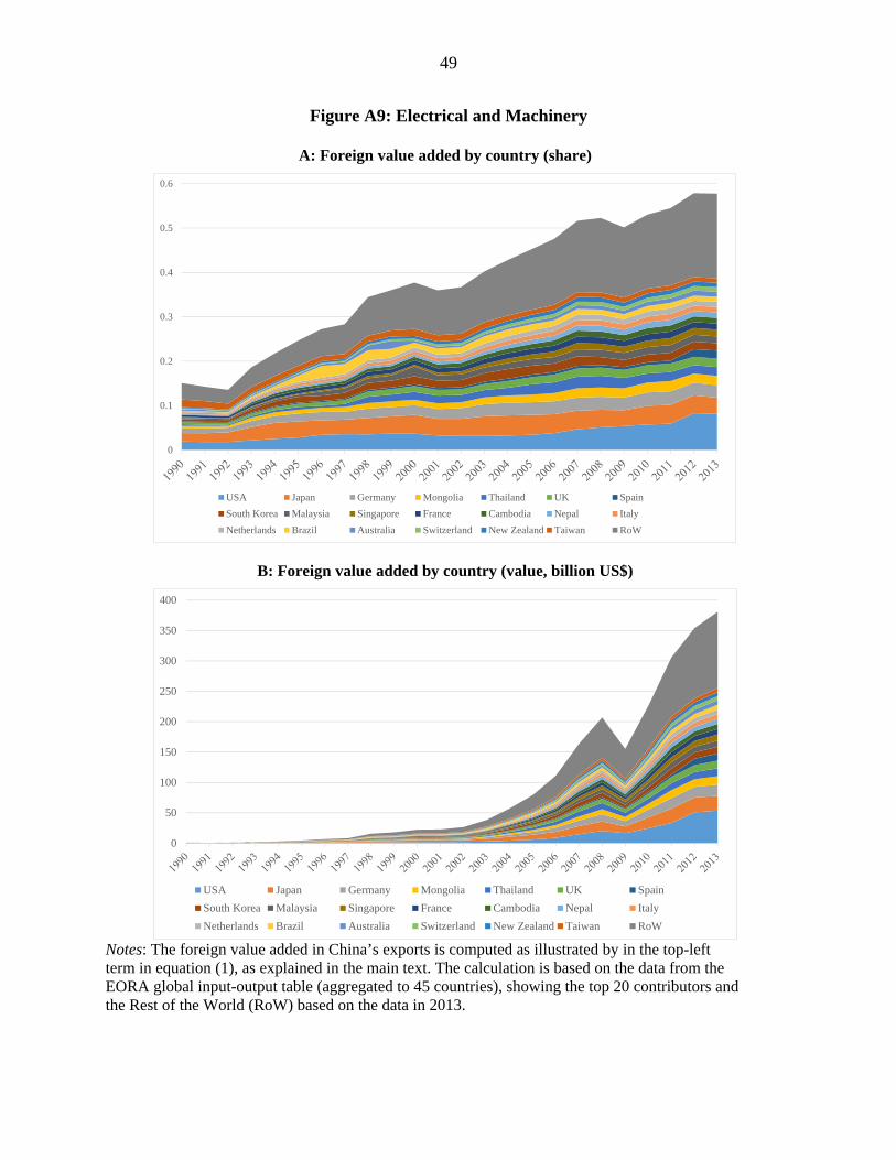
49

Figure A9: Electrical and Machinery

A: Foreign value added by country (share)

0

0.1

0.2

0.3

0.4

0.5

0.6

USA Japan Germany Mongolia Thailand UK Spain

South Korea Malaysia Singapore France Cambodia Nepal Italy

Netherlands Brazil Australia Switzerland New Zealand Taiwan RoW

B: Foreign value added by country (value, billion US$)

0

50

100

150

200

250

300

350

400

USA Japan Germany Mongolia Thailand UK Spain

South Korea Malaysia Singapore France Cambodia Nepal Italy

Netherlands Brazil Australia Switzerland New Zealand Taiwan RoW

Notes: The foreign value added in China’s exports is computed as illustrated by in the top-left term in equation (1), as explained in the main text. The calculation is based on the data from the EORA global input-output table (aggregated to 45 countries), showing the top 20 contributors and the Rest of the World (RoW) based on the data in 2013.

50

Figure A10: Transport Equipment

A: Foreign value added by country (share)

0

0.05

0.1

0.15

0.2

0.25

0.3

USA Japan South Korea Germany Viet Nam Spain Singapore

Malaysia UK Indonesia Australia North Korea France Taiwan

Switzerland Mongolia Italy Thailand Netherlands Philippines RoW

B: Foreign value added by country (value, billion US$)

0

0.5

1

1.5

2

2.5

3

3.5

4

4.5

USA Japan South Korea Germany Viet Nam Spain Singapore

Malaysia UK Indonesia Australia North Korea France Taiwan

Switzerland Mongolia Italy Thailand Netherlands Philippines RoW

Notes: The foreign value added in China’s exports is computed as illustrated by in the top-left term in equation (1), as explained in the main text. The calculation is based on the data from the EORA global input-output table (aggregated to 45 countries), showing the top 20 contributors and the Rest of the World (RoW) based on the data in 2013.

51

Appendix B: Ad valorem tariff rates in China

We use the data on Harmonized System 2-digit level Chinese tariff rates from the Tariff

Analysis Online Facility provided by WTO (TAO, http://tao.wto.org/ ). The downloaded tariffs

are the “MFN Applied Duty Rates” and available for 97 products for 1996, 1997 and 2001-2013.

We calculate the simple average tariff rate for each of 11 traded EORA sectors using the tariff

data for 97 products. The resulting ad valorem tariff rates are shown in Table B1.

Figure B1: The Chinese tariff rates (in %) for 10 sectors in EORA

Notes: The vertical axis measures the tariff rate (in %).