Statistics review 8: Qualitative data – tests of association

46

Critical Care February 2004 Vol 8 No 1 Bewick et al.

Introduction

In the previous statistics reviews most of the procedures dis-cussed are appropriate for quantitative measurements.However, qualitative, or categorical, data are frequently col-lected in medical investigations. For example, variablesassessed might include sex, blood group, classification ofdisease, or whether the patient survived. Categorical vari-ables may also comprise grouped quantitative variables; forexample, age could be grouped into ‘under 20 years’,‘20–50 years’ and ‘over 50 years’. Some categorical variablesmay be ordinal, that is the data arising can be ordered. Agegroup is an example of an ordinal categorical variable.

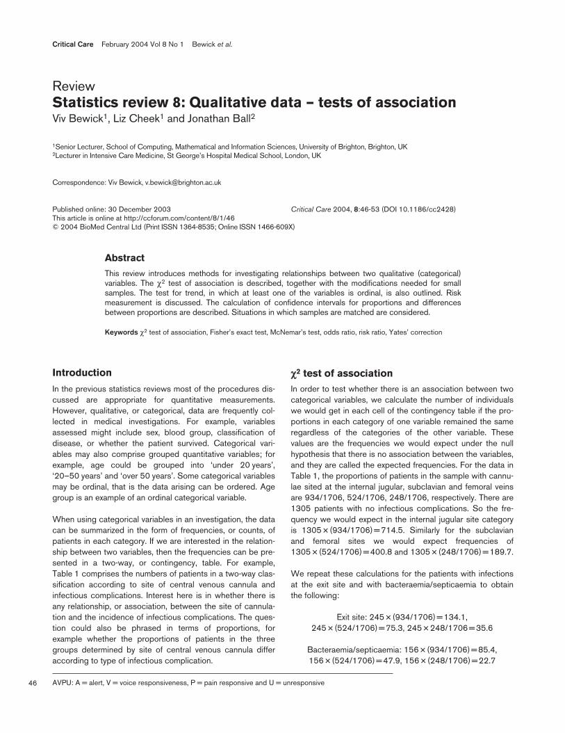
When using categorical variables in an investigation, the datacan be summarized in the form of frequencies, or counts, ofpatients in each category. If we are interested in the relation-ship between two variables, then the frequencies can be pre-sented in a two-way, or contingency, table. For example,Table 1 comprises the numbers of patients in a two-way clas-sification according to site of central venous cannula andinfectious complications. Interest here is in whether there isany relationship, or association, between the site of cannula-tion and the incidence of infectious complications. The ques-tion could also be phrased in terms of proportions, forexample whether the proportions of patients in the threegroups determined by site of central venous cannula differaccording to type of infectious complication.

χχ2 test of association

In order to test whether there is an association between twocategorical variables, we calculate the number of individualswe would get in each cell of the contingency table if the pro-portions in each category of one variable remained the sameregardless of the categories of the other variable. Thesevalues are the frequencies we would expect under the nullhypothesis that there is no association between the variables,and they are called the expected frequencies. For the data inTable 1, the proportions of patients in the sample with cannu-lae sited at the internal jugular, subclavian and femoral veinsare 934/1706, 524/1706, 248/1706, respectively. There are1305 patients with no infectious complications. So the fre-quency we would expect in the internal jugular site categoryis 1305 × (934/1706) = 714.5. Similarly for the subclavianand femoral sites we would expect frequencies of1305 × (524/1706) = 400.8 and 1305 × (248/1706) = 189.7.

We repeat these calculations for the patients with infectionsat the exit site and with bacteraemia/septicaemia to obtainthe following:

Exit site: 245 × (934/1706) = 134.1,245 × (524/1706) = 75.3, 245 × 248/1706 = 35.6

Bacteraemia/septicaemia: 156 × (934/1706) = 85.4,156 × (524/1706) = 47.9, 156 × (248/1706) = 22.7

ReviewStatistics review 8: Qualitative data – tests of associationViv Bewick1, Liz Cheek1 and Jonathan Ball2

1Senior Lecturer, School of Computing, Mathematical and Information Sciences, University of Brighton, Brighton, UK2Lecturer in Intensive Care Medicine, St George’s Hospital Medical School, London, UK

Correspondence: Viv Bewick, [email protected]

Published online: 30 December 2003 Critical Care 2004, 8:46-53 (DOI 10.1186/cc2428)This article is online at http://ccforum.com/content/8/1/46© 2004 BioMed Central Ltd (Print ISSN 1364-8535; Online ISSN 1466-609X)

Abstract

This review introduces methods for investigating relationships between two qualitative (categorical)variables. The χ2 test of association is described, together with the modifications needed for smallsamples. The test for trend, in which at least one of the variables is ordinal, is also outlined. Riskmeasurement is discussed. The calculation of confidence intervals for proportions and differencesbetween proportions are described. Situations in which samples are matched are considered.

Keywords χ2 test of association, Fisher’s exact test, McNemar’s test, odds ratio, risk ratio, Yates’ correction

AVPU: A = alert, V = voice responsiveness, P = pain responsive and U = unresponsive

47

Available online http://ccforum.com/content/8/1/46

We thus obtain a table of expected frequencies (Table 2).Note that 1305 × (934/1706) is the same as934 × (1305/8766), and so equally we could have wordedthe argument in terms of proportions of patients in each ofthe infectious complications categories remaining constantfor each central line site. In each case, the calculation is con-ditional on the sizes of the row and column totals and on thetotal sample size.

The test of association involves calculating the differencesbetween the observed and expected frequencies. If the differ-ences are large, then this suggests that there is an associa-tion between one variable and the other. The difference foreach cell of the table is scaled according to the expected fre-quency in the cell. The calculated test statistic for a table withr rows and c columns is given by:

where Oij is the observed frequency and Eij is the expectedfrequency in the cell in row i and column j. If the null hypothe-sis of no association is true, then the calculated test statisticapproximately follows a χ2 distribution with (r – 1) × (c – 1)degrees of freedom (where r is the number of rows and c thenumber of columns). This approximation can be used toobtain a P value.

For the data in Table 1, the test statistic is:

1.134 + 2.380 + 1.314 + 6.279 + 21.531 +2.052 + 2.484 + 14.069 + 0.020 = 51.26

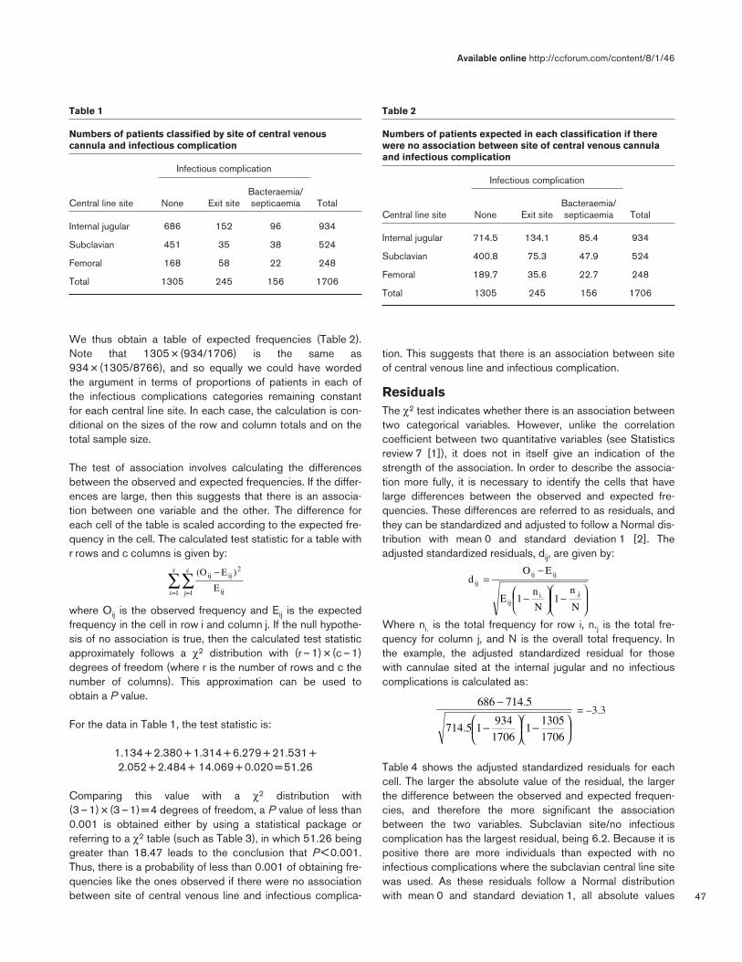
Comparing this value with a χ2 distribution with(3 – 1) × (3 – 1) = 4 degrees of freedom, a P value of less than0.001 is obtained either by using a statistical package orreferring to a χ2 table (such as Table 3), in which 51.26 beinggreater than 18.47 leads to the conclusion that P < 0.001.Thus, there is a probability of less than 0.001 of obtaining fre-quencies like the ones observed if there were no associationbetween site of central venous line and infectious complica-

tion. This suggests that there is an association between siteof central venous line and infectious complication.

ResidualsThe χ2 test indicates whether there is an association betweentwo categorical variables. However, unlike the correlationcoefficient between two quantitative variables (see Statisticsreview 7 [1]), it does not in itself give an indication of thestrength of the association. In order to describe the associa-tion more fully, it is necessary to identify the cells that havelarge differences between the observed and expected fre-quencies. These differences are referred to as residuals, andthey can be standardized and adjusted to follow a Normal dis-tribution with mean 0 and standard deviation 1 [2]. Theadjusted standardized residuals, dij, are given by:

Where ni. is the total frequency for row i, n.j is the total fre-quency for column j, and N is the overall total frequency. Inthe example, the adjusted standardized residual for thosewith cannulae sited at the internal jugular and no infectiouscomplications is calculated as:

= –3.3

Table 4 shows the adjusted standardized residuals for eachcell. The larger the absolute value of the residual, the largerthe difference between the observed and expected frequen-cies, and therefore the more significant the associationbetween the two variables. Subclavian site/no infectiouscomplication has the largest residual, being 6.2. Because it ispositive there are more individuals than expected with noinfectious complications where the subclavian central line sitewas used. As these residuals follow a Normal distributionwith mean 0 and standard deviation 1, all absolute values

Table 1

Numbers of patients classified by site of central venouscannula and infectious complication

Infectious complication

Bacteraemia/Central line site None Exit site septicaemia Total

Internal jugular 686 152 96 934

Subclavian 451 35 38 524

Femoral 168 58 22 248

Total 1305 245 156 1706

Table 2

Numbers of patients expected in each classification if therewere no association between site of central venous cannulaand infectious complication


Bacteraemia/Central line site None Exit site septicaemia Total

Internal jugular 714.5 134.1 85.4 934

Subclavian 400.8 75.3 47.9 524

Femoral 189.7 35.6 22.7 248

Total 1305 245 156 1706

∑∑= =

−r

1i

c

1j ij

2ijij

E

)E(O

−

−

−=

N

n1

N

n1E

EOd

.ji.ij

ijijij

−

−

−

1706

13051

1706

93415.714

5.714686

48


over 2 are significant (see Statistics review 2 [3]). The associ-ation between femoral site/no infectious complication is alsosignificant, but because the residual is negative there arefewer individuals than expected in this cell. When the subcla-vian central line site was used infectious complications appearto be less likely than when the other two sites were used.

Two by two tablesThe use of the χ2 distribution in tests of association is anapproximation that depends on the expected frequenciesbeing reasonably large. When the relationship between twocategorical variables, each with only two categories, is beinginvestigated, variations on the χ2 test of association are oftencalculated as well as, or instead of, the usual test in order toimprove the approximation. Table 5 comprises data onpatients with acute myocardial infarction who took part in atrial of intravenous nitrate (see Statistics review 3 [4]). A totalof 50 patients were randomly allocated to the treatment

group and 45 to the control group. The table shows thenumbers of patients who died and survived in each group.Theχ2 test gives a test statistic of 3.209 with 1 degree offreedom and a P value of 0.073. This suggests there is notenough evidence to indicate an association between treat-ment and survival.

Fisher’s exact test

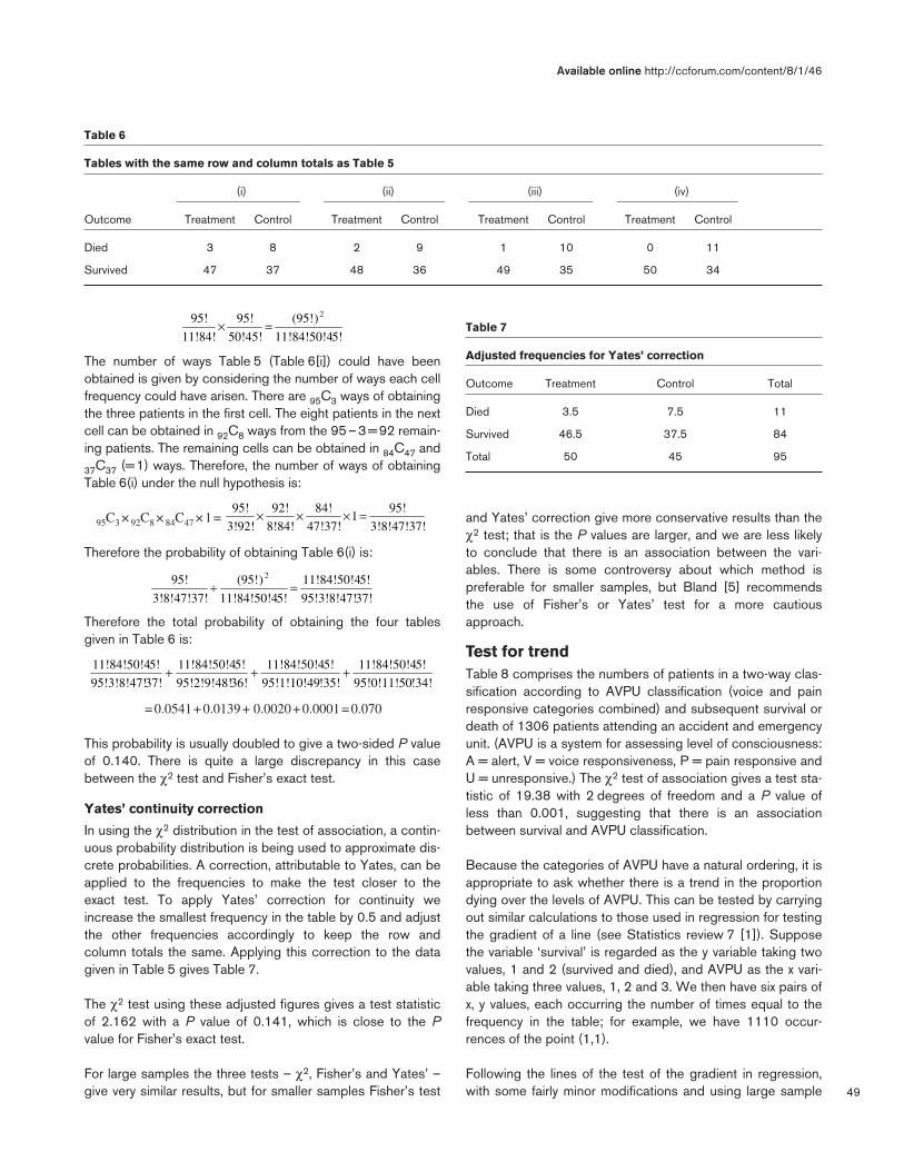
The exact P value for a two by two table can be calculated byconsidering all the tables with the same row and columntotals as the original but which are as or more extreme in theirdeparture from the null hypothesis. In the case of Table 5, weconsider all the tables in which three or fewer patients receiv-ing the treatment died, given in Table 6(i)–(iv). The exactprobabilities of obtaining each of these tables under the nullhypothesis of no association or independence between treat-ment and survival are obtained as follows.

To calculate the probability of obtaining a particular table, weconsider the total number of possible tables with the givenmarginal totals, and the number of ways we could haveobtained the particular cell frequencies in the table in ques-tion. The number of ways the row totals of 11 and 84 couldhave been obtained given 95 patients altogether is denotedby 95C11 and is equal to 95!/11!84!, where 95! (‘95 factorial’)is the product of 95 and all the integers lower than itselfdown to 1. Similarly the number of ways the column totals of50 and 45 could have been obtained is given by

95C50 = 95!/50!45!. Assuming independence, the totalnumber of possible tables with the given marginal totals is:

Table 3

Percentage points of the χ2 distribution produced on aspreadsheet

χ2 values for the probabilities (P)

Degreesof freedom 0.1 0.05 0.01 0.001

1 2.71 3.84 6.63 10.83

2 4.61 5.99 9.21 13.82

3 6.25 7.81 11.34 16.27

4 7.78 9.49 13.28 18.47

5 9.24 11.07 15.09 20.52

6 10.64 12.59 16.81 22.46

7 12.02 14.07 18.48 24.32

8 13.36 15.51 20.09 26.12

9 14.68 16.92 21.67 27.88

10 15.99 18.31 23.21 29.59

11 17.28 19.68 24.72 31.26

12 18.55 21.03 26.22 32.91

13 19.81 22.36 27.69 34.53

14 21.06 23.68 29.14 36.12

15 22.31 25.00 30.58 37.70

16 23.54 26.30 32.00 39.25

17 24.77 27.59 33.41 40.79

18 25.99 28.87 34.81 42.31

19 27.20 30.14 36.19 43.82

20 28.41 31.41 37.57 45.31

25 34.38 37.65 44.31 52.62

Table 4

The adjusted standardized residuals


Bacteraemia/Central line site None Exit site septicaemia

Internal jugular –3.3 2.5 1.8

Subclavian 6.2 –6.0 –1.8

Femoral –3.5 4.4 –0.2

Table 5

Data on patients with acute myocardial infarction who tookpart in a trial of intravenous nitrate

Outcome Treatment Control Total

Died 3 8 11

Survived 47 37 84

Total 50 45 95

49

The number of ways Table 5 (Table 6[i]) could have beenobtained is given by considering the number of ways each cellfrequency could have arisen. There are 95C3 ways of obtainingthe three patients in the first cell. The eight patients in the nextcell can be obtained in 92C8 ways from the 95–3=92 remain-ing patients. The remaining cells can be obtained in 84C47 and

37C37 (=1) ways. Therefore, the number of ways of obtainingTable 6(i) under the null hypothesis is:

95C3 × 92C8 × 84C47 ×1=

Therefore the probability of obtaining Table 6(i) is:

Therefore the total probability of obtaining the four tablesgiven in Table 6 is:

=0.0541+0.0139+ 0.0020+0.0001=0.070

This probability is usually doubled to give a two-sided P valueof 0.140. There is quite a large discrepancy in this casebetween the χ2 test and Fisher’s exact test.

Yates’ continuity correction

In using the χ2 distribution in the test of association, a contin-uous probability distribution is being used to approximate dis-crete probabilities. A correction, attributable to Yates, can beapplied to the frequencies to make the test closer to theexact test. To apply Yates’ correction for continuity weincrease the smallest frequency in the table by 0.5 and adjustthe other frequencies accordingly to keep the row andcolumn totals the same. Applying this correction to the datagiven in Table 5 gives Table 7.

The χ2 test using these adjusted figures gives a test statisticof 2.162 with a P value of 0.141, which is close to the Pvalue for Fisher’s exact test.

For large samples the three tests – χ2, Fisher’s and Yates’ –give very similar results, but for smaller samples Fisher’s test

and Yates’ correction give more conservative results than theχ2 test; that is the P values are larger, and we are less likelyto conclude that there is an association between the vari-ables. There is some controversy about which method ispreferable for smaller samples, but Bland [5] recommendsthe use of Fisher’s or Yates’ test for a more cautiousapproach.

Test for trendTable 8 comprises the numbers of patients in a two-way clas-sification according to AVPU classification (voice and painresponsive categories combined) and subsequent survival ordeath of 1306 patients attending an accident and emergencyunit. (AVPU is a system for assessing level of consciousness:A = alert, V = voice responsiveness, P = pain responsive andU = unresponsive.) The χ2 test of association gives a test sta-tistic of 19.38 with 2 degrees of freedom and a P value ofless than 0.001, suggesting that there is an associationbetween survival and AVPU classification.

Because the categories of AVPU have a natural ordering, it isappropriate to ask whether there is a trend in the proportiondying over the levels of AVPU. This can be tested by carryingout similar calculations to those used in regression for testingthe gradient of a line (see Statistics review 7 [1]). Supposethe variable ‘survival’ is regarded as the y variable taking twovalues, 1 and 2 (survived and died), and AVPU as the x vari-able taking three values, 1, 2 and 3. We then have six pairs ofx, y values, each occurring the number of times equal to thefrequency in the table; for example, we have 1110 occur-rences of the point (1,1).

Following the lines of the test of the gradient in regression,with some fairly minor modifications and using large sample


Table 6

Tables with the same row and column totals as Table 5

(i) (ii) (iii) (iv)

Outcome Treatment Control Treatment Control Treatment Control Treatment Control

Died 3 8 2 9 1 10 0 11

Survived 47 37 48 36 49 35 50 34

Table 7

Adjusted frequencies for Yates’ correction

Outcome Treatment Control Total

Died 3.5 7.5 11

Survived 46.5 37.5 84

Total 50 45 95

5!11!84!50!4

)(95!

50!45!

95!

11!84!

95! 2

=×

3!8!47!37!

95!1

47!37!

84!

8!84!

92!

3!92!

95! =×××

!34!95!0!11!50

5!11!84!50!4

!35!95!1!10!49

5!11!84!50!4

36!95!2!9!48!

5!11!84!50!4

37!95!3!8!47!

5!11!84!50!4 +++

37!95!3!8!47!

5!11!84!50!4

5!11!84!50!4

)(95!

3!8!47!37!

95! 2

=÷

50

approximations, we obtain a χ2 statistic with 1 degree offreedom given by [5]:

For the data in Table 8, we obtain a test statistic of 19.33with 1 degree of freedom and a P value of less than 0.001.Therefore, the trend is highly significant. The differencebetween the χ2 test statistic for trend and the χ2 test statisticin the original test is 19.38 – 19.33 = 0.05 with 2 – 1 = 1degree of freedom, which provides a test of the departurefrom the trend. This departure is very insignificant and sug-gests that the association between survival and AVPU classi-fication can be explained almost entirely by the trend.

Some computer packages give the trend test, or a variation.The trend test described above is sometimes called theCochran–Armitage test, and a common variation is theMantel–Haentzel trend test.

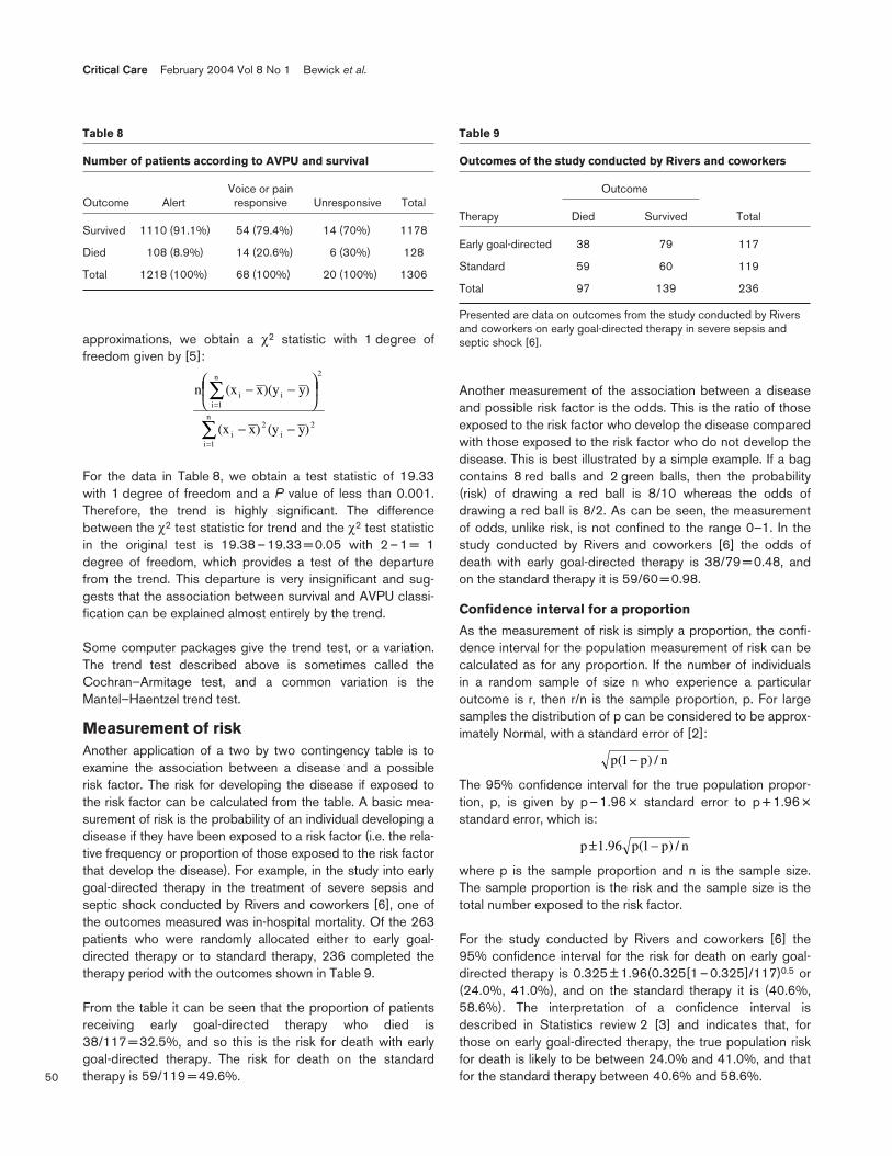
Measurement of riskAnother application of a two by two contingency table is toexamine the association between a disease and a possiblerisk factor. The risk for developing the disease if exposed tothe risk factor can be calculated from the table. A basic mea-surement of risk is the probability of an individual developing adisease if they have been exposed to a risk factor (i.e. the rela-tive frequency or proportion of those exposed to the risk factorthat develop the disease). For example, in the study into earlygoal-directed therapy in the treatment of severe sepsis andseptic shock conducted by Rivers and coworkers [6], one ofthe outcomes measured was in-hospital mortality. Of the 263patients who were randomly allocated either to early goal-directed therapy or to standard therapy, 236 completed thetherapy period with the outcomes shown in Table 9.

From the table it can be seen that the proportion of patientsreceiving early goal-directed therapy who died is38/117 = 32.5%, and so this is the risk for death with earlygoal-directed therapy. The risk for death on the standardtherapy is 59/119 = 49.6%.

Another measurement of the association between a diseaseand possible risk factor is the odds. This is the ratio of thoseexposed to the risk factor who develop the disease comparedwith those exposed to the risk factor who do not develop thedisease. This is best illustrated by a simple example. If a bagcontains 8 red balls and 2 green balls, then the probability(risk) of drawing a red ball is 8/10 whereas the odds ofdrawing a red ball is 8/2. As can be seen, the measurementof odds, unlike risk, is not confined to the range 0–1. In thestudy conducted by Rivers and coworkers [6] the odds ofdeath with early goal-directed therapy is 38/79 = 0.48, andon the standard therapy it is 59/60 = 0.98.

Confidence interval for a proportion

As the measurement of risk is simply a proportion, the confi-dence interval for the population measurement of risk can becalculated as for any proportion. If the number of individualsin a random sample of size n who experience a particularoutcome is r, then r/n is the sample proportion, p. For largesamples the distribution of p can be considered to be approx-imately Normal, with a standard error of [2]:

The 95% confidence interval for the true population propor-tion, p, is given by p – 1.96 × standard error to p + 1.96 ×standard error, which is:

where p is the sample proportion and n is the sample size.The sample proportion is the risk and the sample size is thetotal number exposed to the risk factor.

For the study conducted by Rivers and coworkers [6] the95% confidence interval for the risk for death on early goal-directed therapy is 0.325 ± 1.96(0.325[1 – 0.325]/117)0.5 or(24.0%, 41.0%), and on the standard therapy it is (40.6%,58.6%). The interpretation of a confidence interval isdescribed in Statistics review 2 [3] and indicates that, forthose on early goal-directed therapy, the true population riskfor death is likely to be between 24.0% and 41.0%, and thatfor the standard therapy between 40.6% and 58.6%.


Table 8

Number of patients according to AVPU and survival

Voice or painOutcome Alert responsive Unresponsive Total

Survived 1110 (91.1%) 54 (79.4%) 14 (70%) 1178

Died 108 (8.9%) 14 (20.6%) 6 (30%) 128

Total 1218 (100%) 68 (100%) 20 (100%) 1306

Table 9

Outcomes of the study conducted by Rivers and coworkers

Outcome

Therapy Died Survived Total

Early goal-directed 38 79 117

Standard 59 60 119

Total 97 139 236

Presented are data on outcomes from the study conducted by Riversand coworkers on early goal-directed therapy in severe sepsis andseptic shock [6].

∑

∑

=

=

−−

−−

n

1i

2i

2i

2n

1iii

)y(y)x(x

)y)(yx(xn

n/)p1(p96.1p −±

n/)p1(p −

51

Comparing risksTo assess the importance of the risk factor, it is necessary tocompare the risk for developing a disease in the exposedgroup with the risk in the nonexposed group. In the study byRivers and coworkers [6] the risk for death on the early goal-directed therapy is 32.5%, whereas on the standard therapy itis 49.6%. A comparison between the two risks can be madeby examining either their ratio or the difference between them.

Risk ratio

The risk ratio measures the increased risk for developing adisease when having been exposed to a risk factor comparedwith not having been exposed to the risk factor. It is given byRR = risk for the exposed/risk for the unexposed, and it isoften referred to as the relative risk. The interpretation of a rel-ative risk is described in Statistics review 6 [7]. For the Riversstudy the relative risk = 0.325/0.496 = 0.66, which indicatesthat a patient on the early goal-directed therapy is 34% lesslikely to die than a patient on the standard therapy.

The calculation of the 95% confidence interval for the relativerisk [8] will be covered in a future review, but it can usefullybe interpreted here. For the Rivers study the 95% confidenceinterval for the population relative risk is 0.48 to 0.90.Because the interval does not contain 1.0 and the upper endis below, it indicates that patients on the early goal-directedtherapy have a significantly decreased risk for dying as com-pared with those on the standard therapy.

Odds ratio

When quantifying the risk for developing a disease, the ratioof the odds can also be used as a measurement of compari-son between those exposed and not exposed to a risk factor.It is given by OR = odds for the exposed/odds for the unex-posed, and is referred to as the odds ratio. The interpretationof odds ratio is described in Statistics review 3 [4]. For theRivers study the odds ratio = 0.48/0.98 = 0.49, again indicat-ing that those on the early goal-directed therapy have areduced risk for dying as compared with those on the stan-dard therapy. This will be covered fully in a future review.

The calculation of the 95% confidence interval for the oddsratio [2] will also be covered in a future review but, as withrelative risk, it can usefully be interpreted here. For the Riversexample the 95% confidence interval for the odds ratio is0.29 to 0.83. This can be interpreted in the same way as the95% confidence interval for the relative risk, indicating thatthose receiving early goal-directed therapy have a reducedrisk for dying.

Difference between two proportionsConfidence intervalFor the Rivers study, instead of examining the ratio of therisks (the relative risk) we can obtain a confidence intervaland carry out a significance test of the difference betweenthe risks. The proportion of those on early goal-directed

therapy who died is p1 = 38/117 = 0.325 and the proportionof those on standard therapy who died isp2 = 59/119 = 0.496. A confidence interval for the differencebetween the true population proportions is given by:

(p1 – p2) – 1.96 × se(p1 – p2) to (p1 – p2) + 1.96 × se(p1 – p2)

Where se(p1 – p2) is the standard error of p1 – p2 and is cal-culated as:

= = 0.063

Thus, the required confidence interval is –0.171 – 1.96 ×0.063 to –0.171 + 1.96 × 0.063; that is –0.295 to –0.047.Therefore, the difference between the true proportions islikely to be between –0.295 and –0.047, and the risk forthose on early goal-directed therapy is less than the risk forthose on standard therapy.

Hypothesis test

We can also carry out a hypothesis test of the null hypothesisthat the difference between the proportions is 0. This followssimilar lines to the calculation of the confidence interval, butunder the null hypothesis the standard error of the differencein proportions is given by:

=

where p is a pooled estimate of the proportion obtained fromboth samples [5]:

= = 0.3856

So:

se(p1 – p2) = = 0.0634

The test statistic is then:

= –2.71

Comparing this value with a standard Normal distributiongives p = 0.007, again suggesting that there is a differencebetween the two population proportions. In fact, the testdescribed is equivalent to the χ2 test of association on thetwo by two table. The χ2 test gives a test statistic of 7.31,which is equal to (–2.71)2 and has the same P value of0.007. Again, this suggests that there is a difference betweenthe risks for those receiving early goal-directed therapy andthose receiving standard therapy.

Matched samplesMatched pair designs, as discussed in Statistics review 5 [9],can also be used when the outcome is categorical. For


2n

)2p(12p

1n

)1p(11p −+

−

119

0.5040.496

117

0.6750.325 ×+

×

2n

)2p(12p

1n

)1p(11p −+

−

+−

21 n

1

n

1p)p(1

sizes sample of total

samplesboth in deaths total

236

97

119117

5938=

+

+

+××

119

1

117

10.61440.3856

0.0634

0.1710-

)2p1se(p2p1p

=−

−

52

example, when comparing two tests to determine a particularcondition, the same individuals can be used for each test.

McNemar’s test

In this situation, because the χ2 test does not take pairing intoconsideration, a more appropriate test, attributed toMcNemar, can be used when comparing these correlatedproportions.

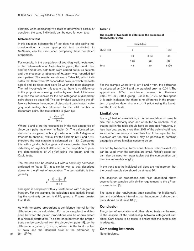
For example, in the comparison of two diagnostic tests usedin the determination of Helicobacter pylori, the breath testand the Oxoid test, both tests were carried out in 84 patientsand the presence or absence of H. pylori was recorded foreach patient. The results are shown in Table 10, which indi-cates that there were 72 concordant pairs (in which the testsagree) and 12 discordant pairs (in which the tests disagree).The null hypothesis for this test is that there is no differencein the proportions showing positive by each test. If this weretrue then the frequencies for the two categories of discordantpairs should be equal [5]. The test involves calculating the dif-ference between the number of discordant pairs in each cate-gory and scaling this difference by the total number ofdiscordant pairs. The test statistic is given by:

Where b and c are the frequencies in the two categories ofdiscordant pairs (as shown in Table 10). The calculated teststatistic is compared with a χ2 distribution with 1 degree offreedom to obtain a P value. For the example b = 8 and c = 4,therefore the test statistic is calculated as 1.33. Comparingthis with a χ2 distribution gives a P value greater than 0.10,indicating no significant difference in the proportion of posi-tive determinations of H. pylori using the breath and theOxoid tests.

The test can also be carried out with a continuity correctionattributed to Yates [5], in a similar way to that describedabove for the χ2 test of association. The test statistic is thengiven by:

and again is compared with a χ2 distribution with 1 degree offreedom. For the example, the calculated test statistic includ-ing the continuity correct is 0.75, giving a P value greaterthan 0.25.

As with nonpaired proportions a confidence interval for thedifference can be calculated. For large samples the differ-ence between the paired proportions can be approximatedto a Normal distribution. The difference between the propor-tions can be calculated from the discordant pairs [8], so thedifference is given by (b – c)/n, where n is the total numberof pairs, and the standard error of the difference by(b + c)0.5/n.

For the example where b = 8, c = 4 and n = 84, the differenceis calculated as 0.048 and the standard error as 0.041. Theapproximate 95% confidence interval is therefore0.048 ± 1.96 × 0.041 giving –0.033 to 0.129. As this spans0, it again indicates that there is no difference in the propor-tion of positive determinations of H. pylori using the breathand the Oxoid tests.

LimitationsFor a χ2 test of association, a recommendation on samplesize that is commonly used and attributed to Cochran [5] isthat no cell in the table should have an expected frequency ofless than one, and no more than 20% of the cells should havean expected frequency of less than five. If the expected fre-quencies are too small then it may be possible to combinecategories where it makes sense to do so.

For two by two tables, Yates’ correction or Fisher’s exact testcan be used when the samples are small. Fisher’s exact testcan also be used for larger tables but the computation canbecome impossibly lengthy.

In the trend test the individual cell sizes are not important butthe overall sample size should be at least 30.

The analyses of proportions and risks described aboveassume large samples with similar requirement to the χ2 testof association [8].

The sample size requirement often specified for McNemar’stest and confidence interval is that the number of discordantpairs should be at least 10 [8].

ConclusionThe χ2 test of association and other related tests can be usedin the analysis of the relationship between categorical vari-ables. Care needs to be taken to ensure that the sample sizeis adequate.

Competing interestsNone declared.


Table 10

The results of two tests to determine the presence ofHelicobacter pylori

Breath test

Oxoid test + – Total

+ 40 8 (b) 48

– 4 (c) 32 36

Total 44 40 84(n)

cb

)cb( 22

+−=χ

( )cb

1cb 22

+−−

=χ

53

References1. Bewick V, Cheek L, Ball J: Statistics review 7: Correlation and

regression. Crit Care 2003, 7:451-459.2. Everitt BS: The Analysis of Contingency Tables, 2nd ed. London,

UK: Chapman & Hall; 1992.3. Whitley E, Ball J: Statistics review 2: samples and populations.

Crit Care 2002, 6:143-148.4. Whitley E, Ball J: Statistics review 3: hypothesis testing and P

values. Crit Care 2002, 6:222-225.5. Bland M: An Introduction to Medical Statistics, 3rd ed. Oxford,

UK: Oxford University Press; 2001.6. Rivers E, Nguyen B, Havstad S, Ressler J, Muzzin A, Knoblich B,

Peterson E, Tomlanovich M; Early Goal-Directed Therapy Collabo-rative Group: Early goal-directed therapy in the treatment ofsevere sepsis and septic shock. N Engl J Med 2001,345:1368-1377.

7. Whitley E, Ball J: Statistics review 6: Nonparametric methods.Crit Care 2002, 6:509-513.

8. Kirkwood BR, Sterne JAC: Essential Medical Statistics, 2nd ed.Oxford, UK: Blackwell Science Ltd; 2003.

9. Whitley E, Ball J: Statistics review 5: Comparison of means.Crit Care 2002, 6:424-428.


This article is the eighth in an ongoing, educational reviewseries on medical statistics in critical care.

Previous articles have covered ‘presenting andsummarizing data’, ‘samples and populations’, ‘hypothesestesting and P values’, ‘sample size calculations’,‘comparison of means’, ‘nonparametric means’ and‘correlation and regression’.

Future topics to be covered include:

Chi-squared and Fishers exact testsAnalysis of varianceFurther non-parametric tests: Kruskal–Wallis and FriedmanMeasures of disease: PR/ORSurvival data: Kaplan–Meier curves and log rank testsROC curvesMultiple logistic regression.

If there is a medical statistics topic you would likeexplained, contact us at [email protected].

Documents

Statistics review 8: Qualitative data – tests of association