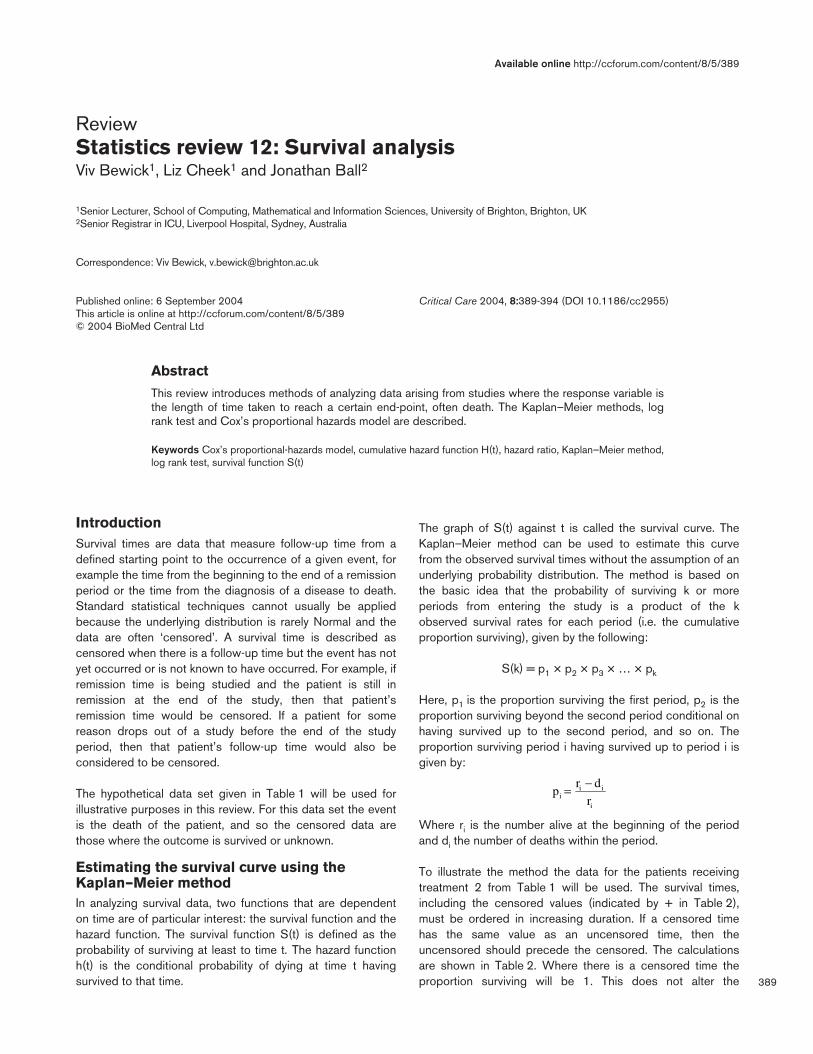
389

Available online http://ccforum.com/content/8/5/389

IntroductionSurvival times are data that measure follow-up time from adefined starting point to the occurrence of a given event, forexample the time from the beginning to the end of a remissionperiod or the time from the diagnosis of a disease to death.Standard statistical techniques cannot usually be appliedbecause the underlying distribution is rarely Normal and thedata are often ‘censored’. A survival time is described ascensored when there is a follow-up time but the event has notyet occurred or is not known to have occurred. For example, ifremission time is being studied and the patient is still inremission at the end of the study, then that patient’sremission time would be censored. If a patient for somereason drops out of a study before the end of the studyperiod, then that patient’s follow-up time would also beconsidered to be censored.

The hypothetical data set given in Table 1 will be used forillustrative purposes in this review. For this data set the eventis the death of the patient, and so the censored data arethose where the outcome is survived or unknown.

Estimating the survival curve using theKaplan–Meier methodIn analyzing survival data, two functions that are dependenton time are of particular interest: the survival function and thehazard function. The survival function S(t) is defined as theprobability of surviving at least to time t. The hazard functionh(t) is the conditional probability of dying at time t havingsurvived to that time.

The graph of S(t) against t is called the survival curve. TheKaplan–Meier method can be used to estimate this curvefrom the observed survival times without the assumption of anunderlying probability distribution. The method is based onthe basic idea that the probability of surviving k or moreperiods from entering the study is a product of the kobserved survival rates for each period (i.e. the cumulativeproportion surviving), given by the following:

S(k) = p1 × p2 × p3 × … × pk

Here, p1 is the proportion surviving the first period, p2 is theproportion surviving beyond the second period conditional onhaving survived up to the second period, and so on. Theproportion surviving period i having survived up to period i isgiven by:

Where ri is the number alive at the beginning of the periodand di the number of deaths within the period.

To illustrate the method the data for the patients receivingtreatment 2 from Table 1 will be used. The survival times,including the censored values (indicated by + in Table 2),must be ordered in increasing duration. If a censored timehas the same value as an uncensored time, then theuncensored should precede the censored. The calculationsare shown in Table 2. Where there is a censored time theproportion surviving will be 1. This does not alter the

ReviewStatistics review 12: Survival analysisViv Bewick1, Liz Cheek1 and Jonathan Ball2

1Senior Lecturer, School of Computing, Mathematical and Information Sciences, University of Brighton, Brighton, UK2Senior Registrar in ICU, Liverpool Hospital, Sydney, Australia

Correspondence: Viv Bewick, v.bewick@brighton.ac.uk

Published online: 6 September 2004 Critical Care 2004, 8:389-394 (DOI 10.1186/cc2955)This article is online at http://ccforum.com/content/8/5/389© 2004 BioMed Central Ltd

Abstract

This review introduces methods of analyzing data arising from studies where the response variable isthe length of time taken to reach a certain end-point, often death. The Kaplan–Meier methods, logrank test and Cox’s proportional hazards model are described.

Keywords Cox’s proportional-hazards model, cumulative hazard function H(t), hazard ratio, Kaplan–Meier method,log rank test, survival function S(t)

i

iii r

drp

−=

390

Critical Care October 2004 Vol 8 No 5 Bewick et al.

cumulative proportion surviving, and so these calculationscan be omitted from the table. For more detailed explanation,see Swinscow and Campbell [1].

Plotting the cumulative proportion surviving against thesurvival times gives the stepped survival curve shown in Fig. 1.

This method is found in most statistical packages. Figure 2 isthe output from a statistical package used to compare the

survival curves for the two treatment groups for the datagiven in Table 1.

It can be seen that patients on treatment 1 appear to have ahigher survival rate than those on treatment 2. The graph canbe used to estimate the median survival time because this isthe time with probability of survival of 0.5. The median survivaltime for those on treatment 2 appears to be 5 days versusabout 37 days on treatment 1.

Comparing survival curves of two groupsusing the log rank testComparison of two survival curves can be done using astatistical hypothesis test called the log rank test. It is used to

Table 1

Survival time, age and outcome for a group of patientsdiagnosed with a disease and receiving one of two treatments

Patient Survival time Age number (days) Outcome Treatment (years)

1 1 Died 2 75

2 1 Died 2 79

3 4 Died 2 85

4 5 Died 2 76

5 6 Unknown 2 66

6 8 Died 1 75

7 9 Survived 2 72

8 9 Died 2 70

9 12 Died 1 71

10 15 Unknown 1 73

11 22 Died 2 66

12 25 Survived 1 73

13 37 Died 1 68

14 55 Died 1 59

15 72 Survived 1 61

Table 2

Calculations for the Kaplan–Meier estimate of the survival function for the treatment 2 data from Table 1

Survival time Number known Proportion Cumulative proportion Patient number (days) to be alive (ri) Deaths (di) surviving (pi) surviving (S[t])

0 1

1 1 8

2 1 8 2 (8 – 2)/8 = 0.750 1 × 0.750 = 0.750

3 4 6 1 (6 – 1)/6 = 0.833 0.750 × 0.833 = 0.625

4 5 5 1 (5 – 1)/5 = 0.800 0.625 × 0.800 = 0.500

5 6+

7 9 3 1 (3 – 1)/3 = 0.667 0.500 × 0.667 = 0.333

8 9+

11 22 1 1 (1 – 1)/1 = 0.00 0.333 × 0.00 = 0.000

Figure 1

Plot of the survival curve for treatment 2.

Survival time (days)

3020100

Pro

babi

lity

of s

urvi

val

1.0

0.9

0.8

0.7

0.6

0.5

0.4

0.3

0.2

0.1

0

Censored +

391

test the null hypothesis that there is no difference betweenthe population survival curves (i.e. the probability of an eventoccurring at any time point is the same for each population).The test statistic is calculated as follows:

Where the O1 and O2 are the total numbers of observedevents in groups 1 and 2, respectively, and E1 and E2 thetotal numbers of expected events.

The total expected number of events for a group is the sum ofthe expected number of events at the time of each event. Theexpected number of events at the time of an event can becalculated as the risk for death at that time multiplied by thenumber alive in the group. Under the null hypothesis, the riskof death (number of deaths/number alive) can be calculatedfrom the combined data for both groups. Table 3 shows thecalculation of the expected number of deaths for treatmentgroup 2 for the example data. For example, at the beginningof day 4 when the third death (event 3) takes place, there are13 patients still alive. One dies, giving a risk for death of1/13 = 0.077. Six of the 13 patients are from treatmentgroup 2, and therefore the expected number of deaths isgiven by 6 × 0.077 = 0.46 at event 3. The total expectednumber of events for group 2 is calculated as:

Where r2i is the number alive from group 2 at the time ofevent i. E1 can be calculated as n – E2, where n is the totalnumber of events.

The test statistic is compared with a χ2 distribution with 1degree of freedom. It is a simplified version of a statistic thatis often calculated in statistical packages [2].

Available online http://ccforum.com/content/8/5/389

Figure 2

Survival curves for the two treatment groups for the data in Table 1.

Survival time (days)

80706050403020100

Pro

babi

lity

of s

urvi

val

1.0

0.9

0.8

0.7

0.6

0.5

0.4

0.3

0.2

0.1

0

Treatment 2Treatment 1

Censored +

2

222

1

2112

E)E(O

E)E(O

rank) (log×−+−=

Table 3

Calculations for the log-rank test to compare treatments for the data in Table 1

Survival Number Number known Expected number time Treatment known to Deaths Risk for death to be alive from of events in treatment (days) group be alive (ri) (di) (di/ri) treatment group 2 (r2i) group 2 (E2i)

0

1 2 15 2 2/15 = 0.133 8 8 × 0.133 = 1.07

1 2

4 2 13 1 1/13 = 0.077 6 6 × 0.077 = 0.46

5 2 12 1 1/12 = 0.083 5 5 × 0.083 = 0.42

6+ 2 11 0 0/11 = 0 4 4 × 0 = 0.00

8 1 10 1 1/10 = 0.100 3 3 × 0.100 = 0.30

9 2 9 1 1/9 = 0.111 3 3 × 0.111 = 0.33

9+ 2 8 0 0/8 = 0 2 2 × 0 = 0.00

12 1 7 1 1/7 = 0.143 1 1 × 0.143 = 0.14

15+ 1 6 0 0/6 = 0 1 1 × 0 = 0.00

22 2 5 1 1/5 = 0.200 1 1 × 0.200 = 0.20

25+ 1 4 0 0/4 = 0 0 0 × 0 = 0.00

37 1 3 1 1/3 = 0.333 0 0 × 0 = 0.00

55 1 2 1 1/2 = 0.500 0 0 × 0 = 0.00

72+ 1

E2 = 2.92

∑=

=k

1ii2

i

i2 r

rd

E

χ

392

For the data in Table 1, the total number of expected deathsfor treatment group 2 is calculated as 2.92 and the totalnumber of observed deaths is 10, giving a total number ofexpected deaths for treatment group 1 of 10 – 2.92 = 7.08.The value of the test statistic is therefore calculated asfollows:

This gives a P value of 0.032, which indicates a significantdifference between the population survival curves.

An assumption for the log rank test is that of proportionalhazards. This is discussed below. Small departures from thisassumption, however, do not invalidate the test.

Cox’s proportional hazards model (Coxregression)The log rank test is used to test whether there is a differencebetween the survival times of different groups but it does notallow other explanatory variables to be taken into account.

Cox’s proportional hazards model is analogous to a multipleregression model and enables the difference betweensurvival times of particular groups of patients to be testedwhile allowing for other factors. In this model, the response(dependent) variable is the ‘hazard’. The hazard is theprobability of dying (or experiencing the event in question)given that patients have survived up to a given point in time,or the risk for death at that moment.

In Cox’s model no assumption is made about the probabilitydistribution of the hazard. However, it is assumed that if therisk for dying at a particular point in time in one group is, say,twice that in the other group, then at any other time it will stillbe twice that in the other group. In other words, the hazardratio does not depend on time.

The model can be written as:

ln h(t) = ln h0(t) + b1x1 + … + bpxp

or ln = b1x1 + … + bpxp

Where h(t) is the hazard at time t; x1, x2 … xp are theexplanatory variables; and h0(t) is the baseline hazard when allthe explanatory variables are zero. The coefficients b1, b2 … bpare estimated from the data using a statistical package.

Because hazard measures the instantaneous risk for death, itis difficult to illustrate it from sample data. Instead, thecumulative hazard function H(t) can be examined. This can beobtained from the cumulative survival function S(t) as follows:

H(t) = –ln S(t)

The estimated cumulative hazard function for the exampledata given in Table 1 is shown in Table 4.

The assumption that the proportional hazards stay constantover time can be inspected by looking at a graph showing thelogarithm of the estimated cumulative hazard function. Theassumption is equivalent to assuming that the differencebetween the logarithms of the hazards for the two treatmentsdoes not change with time, or equally that the differencebetween the logarithms of the cumulative hazard functions isconstant. Figure 3 is the graph for the example data. The linesfor the two treatments are roughly parallel, suggesting thatthe proportional hazards assumption is reasonable in thiscase. A more formal test of the assumption is possible (seeArmitage and coworkers [2]). Note that, in this graph, thetime scale was also logarithmically transformed. This was tomake the comparison clearer between the two treatments,but it does not affect the vertical positioning of the lines.

Cox’s regression was applied to the example data usingtreatment and age as explanatory variables. The output isshown in Table 5.

The P values indicate that the difference between treatmentswas bordering on statistical significance, whereas there was

Critical Care October 2004 Vol 8 No 5 Bewick et al.

59.492.2

)92.26(

08.7

)08.74( 22

=−+−

(t)h

h(t)

0

Table 4

Cumulative hazard functions (logarithmic scale) for theexample data

Survival time Cumulative survival: Cumulative hazard: (days): t S(t) H(t) = –ln S(t)

Treatment 1

8 0.8571 0.1542

12 0.7143 0.3365

15 0.7143 0.3365

25 0.7143 0.3365

37 0.4762 0.7419

55 0.2381 1.4351

72 0.2381 1.4351

Treatment 2

1

1 0.7500 0.2877

4 0.6250 0.4700

5 0.5000 0.6931

6 0.5000 0.6931

9 0.5000 0.6931

9 0.3333 1.0986

22 0.0000

393

strong evidence that age was associated with length ofsurvival. The coefficient for treatment, –1.887, is thelogarithm of the hazard ratio for a patient given treatment 1compared with a patient given treatment 2 of the same age.The exponential (antilog) of this value is 0.152, indicating thata person receiving treatment 1 is 0.152 times as likely to dieat any time as a patient receiving treatment 2; that is, the riskassociated with treatment 1 appears to be much lower.However, the confidence interval contains 1, indicating thatthere may be no difference in risk associated with the twotreatments.

Using the Kaplan–Meier (log rank) test, the P value for thedifference between treatments was 0.032, whereas usingCox’s regression, and including age as an explanatoryvariable, the corresponding P value was 0.052. This is not asubstantial change and still suggests that a differencebetween treatments is likely. In this case age is clearly animportant explanatory variable and should be included in theanalysis.

The exponential of the coefficient for age, 1.247, indicatesthat a patient 1 year older than another patient, both being

given the same treatment, has an increased risk for dying, bya factor of 1.247. Note that, in this case, the confidenceinterval does not contain 1, indicating the statisticalsignificance of age.

Further models for survival data, allowing for differentassumptions, are discussed by Kirkwood and Sterne [3].

An example from the literatureDupont and coworkers [4] investigated the survival ofpatients with bronchiectasis according to age and use oflong-term oxygen therapy. The Kaplan–Meier curves andresults of the log rank tests shown in Fig. 4 indicate that thereis a significant difference between the survival curves in eachcase.

The authors also applied Cox’s proportional hazards analysisand obtained the results given in Table 6. These resultsindicate that both age and long-term oxygen therapy have asignificant effect on survival. The estimated risk ratio for age,for example, suggests that the risk for death for patients overthe age of 65 years is 2.7 times greater than that for thosebelow 65 years.

Available online http://ccforum.com/content/8/5/389

Figure 3

Cumulative hazard functions for the example data.

Survival time (days) (log scale)

Cum

ulat

ive

haza

rd (

log

scal

e)

100101

1.50

1.000.90

0.80

0.70

0.60

0.50

0.40

0.30

0.20

0.15

Treatment12

Table 5

Application of Cox’s regression to the example data, usingtreatment and age as explanatory variables

95.0% Coefficient Standard confidence

(b) error P eb interval for eb

Treatment –1.887 0.973 0.052 0.152 0.022–1.020

Age 0.220 0.085 0.010 1.247 1.054–1.474

Figure 4

The Kaplan–Meier estimates of survival for (a) age > 65 years or≤65 years, and (b) long-term oxygen therapy (LTOT) before intensivecare unit admission (yes/no). The P values are for the log rank test.

394

Assumptions and limitationsThe log rank test and Cox’s proportional hazards modelassume that the hazard ratio is constant over time. Care mustbe taken to check this assumption.

ConclusionSurvival analysis provides special techniques that arerequired to compare the risks for death (or of some otherevent) associated with different treatments or groups, wherethe risk changes over time. In measuring survival time, thestart and end-points must be clearly defined and thecensored observations noted. Only the most commonly usedtechniques are introduced in this review. Kaplan–Meierprovides a method for estimating the survival curve, the logrank test provides a statistical comparison of two groups, andCox’s proportional hazards model allows additional covariatesto be included. Both of the latter two methods assume thatthe hazard ratio comparing two groups is constant over time.

Competing interestsThe authors declare that they have no competing interests.

References1. Swinscow TDV, Campbell MJ: Statistics at Square One. London:

BMJ Books; 2002.2. Armitage P, Berry G, Matthews JNS: Statistical Methods in

Medical Research, 4th edn. Oxford, UK: Blackwell Science;2002.

3. Kirkwood BR, Sterne JAC: Essential Medical Statistics, 2nd edn.Oxford, UK: Blackwell Science Ltd; 2003.

4. Dupont M, Gacouin A, Lena H, Lavoue S, Brinchault G, Delaval P,Thomas R: Survival of patients with bronchiectasis after thefirst ICU stay for respiratory failure. Chest 2004, 125:1815-1820.

Critical Care October 2004 Vol 8 No 5 Bewick et al.

Table 6

Results of Cox’s proportional hazards analysis for the patientswith bronchiectasis

Explanatory 95% confidence variables Risk ratio interval P

Age (>65 years) 2.7 1.15–6.29 0.022

LTOT (yes) 3.12 1.47–6.90 0.003

LTOT, long-term oxygen therapy.