196 ICU = intensive care unit.

Critical Care June 2004 Vol 8 No 3 Bewick et al.

IntroductionThe previous review in this series [1] described analysis ofvariance, the method used to test for differences betweenmore than two groups or treatments. However, in order to useanalysis of variance, the observations are assumed to havebeen selected from Normally distributed populations withequal variance. The tests described in this review require onlylimited assumptions about the data.

The Kruskal–Wallis test is the nonparametric alternative toone-way analysis of variance, which is used to test fordifferences between more than two populations when thesamples are independent. The Jonckheere–Terpstra test is avariation that can be used when the treatments are ordered.When the samples are related, the Friedman test can be used.

Kruskal–Wallis testThe Kruskal–Wallis test is an extension of the Mann–Whitneytest [2] for more than two independent samples. It is thenonparametric alternative to one-way analysis of variance.Instead of comparing population means, this methodcompares population mean ranks (i.e. medians). For this testthe null hypothesis is that the population medians are equal,versus the alternative that there is a difference between atleast two of them.

The test statistic for one-way analysis of variance iscalculated as the ratio of the treatment sum of squares to theresidual sum of squares [1]. The Kruskal–Wallis test uses thesame method but, as with many nonparametric tests, theranks of the data are used in place of the raw data.

This results in the following test statistic:

Where Rj is the total of the ranks for the jth sample, nj is thesample size for the jth sample, k is the number of samples,and N is the total sample size, given by:

This is approximately distributed as a χ2 distribution with k – 1degrees of freedom. Where there are ties within the data setthe adjusted test statistic is calculated as:

Where rij is the rank for the ith observation in the jth sample,nj is the number of observations in the jth sample, and S2 isgiven by the following:

ReviewStatistics review 10: Further nonparametric methodsViv Bewick1, Liz Cheek2 and Jonathan Ball3

1Senior Lecturer, School of Computing, Mathematical and Information Sciences, University of Brighton, Brighton, UK2Senior Lecturer, School of Computing, Mathematical and Information Sciences, University of Brighton, Brighton, UK3Senior Registrar in ICU, Liverpool Hospital, Sydney, Australia

Corresponding author: Viv Bewick, v.bewick@brighton.ac.uk

Published online: 16 April 2004 Critical Care 2004, 8:196-199 (DOI 10.1186/cc2857)This article is online at http://ccforum.com/content/8/3/196© 2004 BioMed Central Ltd

Abstract

This review introduces nonparametric methods for testing differences between more than two groupsor treatments. Three of the more common tests are described in detail, together with multiplecomparison procedures for identifying specific differences between pairs of groups.

Keywords Friedman test, Jonckheere–Terpstra test, Kruskal–Wallis test, least significant difference

)1(3)1(

12

1

2

+−+

= ∑=

Nn

R

NNT

k

j j

j

∑=

k

jjn

1

.

+−= ∑= 4

)1(1 2

1

2

2

NN

n

R

ST

k

j j

j

197

Available online http://ccforum.com/content/8/3/196

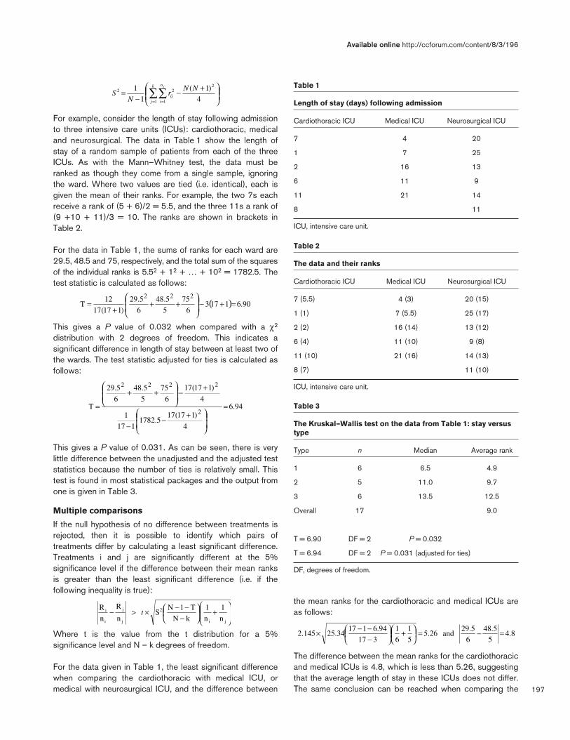
For example, consider the length of stay following admissionto three intensive care units (ICUs): cardiothoracic, medicaland neurosurgical. The data in Table 1 show the length ofstay of a random sample of patients from each of the threeICUs. As with the Mann–Whitney test, the data must beranked as though they come from a single sample, ignoringthe ward. Where two values are tied (i.e. identical), each isgiven the mean of their ranks. For example, the two 7s eachreceive a rank of (5 + 6)/2 = 5.5, and the three 11s a rank of(9 +10 + 11)/3 = 10. The ranks are shown in brackets inTable 2.

For the data in Table 1, the sums of ranks for each ward are29.5, 48.5 and 75, respectively, and the total sum of the squaresof the individual ranks is 5.52 + 12 + … + 102 = 1782.5. Thetest statistic is calculated as follows:

This gives a P value of 0.032 when compared with a χ2

distribution with 2 degrees of freedom. This indicates asignificant difference in length of stay between at least two ofthe wards. The test statistic adjusted for ties is calculated asfollows:

This gives a P value of 0.031. As can be seen, there is verylittle difference between the unadjusted and the adjusted teststatistics because the number of ties is relatively small. Thistest is found in most statistical packages and the output fromone is given in Table 3.

Multiple comparisons

If the null hypothesis of no difference between treatments isrejected, then it is possible to identify which pairs oftreatments differ by calculating a least significant difference.Treatments i and j are significantly different at the 5%significance level if the difference between their mean ranksis greater than the least significant difference (i.e. if thefollowing inequality is true):

Where t is the value from the t distribution for a 5%significance level and N – k degrees of freedom.

For the data given in Table 1, the least significant differencewhen comparing the cardiothoracic with medical ICU, ormedical with neurosurgical ICU, and the difference between

the mean ranks for the cardiothoracic and medical ICUs areas follows:

The difference between the mean ranks for the cardiothoracicand medical ICUs is 4.8, which is less than 5.26, suggestingthat the average length of stay in these ICUs does not differ.The same conclusion can be reached when comparing the

+−−

= ∑∑= =

k

j

n

iij

j NNr

NS

1 1

222

4

)1(

1

1 Table 1

Length of stay (days) following admission

Cardiothoracic ICU Medical ICU Neurosurgical ICU

7 4 20

1 7 25

2 16 13

6 11 9

11 21 14

8 11

ICU, intensive care unit.

Table 2

The data and their ranks

Cardiothoracic ICU Medical ICU Neurosurgical ICU

7 (5.5) 4 (3) 20 (15)

1 (1) 7 (5.5) 25 (17)

2 (2) 16 (14) 13 (12)

6 (4) 11 (10) 9 (8)

11 (10) 21 (16) 14 (13)

8 (7) 11 (10)

ICU, intensive care unit.

Table 3

The Kruskal–Wallis test on the data from Table 1: stay versustype

Type n Median Average rank

1 6 6.5 4.9

2 5 11.0 9.7

3 6 13.5 12.5

Overall 17 9.0

T = 6.90 DF = 2 P = 0.032

T = 6.94 DF = 2 P = 0.031 (adjusted for ties)

DF, degrees of freedom.

( ) 90.611736

75

5

5.48

6

5.29

)117(17

12T

222=+−

++

+=

94.6

4

)117(175.1782

117

1

4

)117(17

6

75

5

5.48

6

5.29

T2

2222

=

+−−

+−

++

=

n

1

n

1

kN

T1NS

n

R

n

R

ji

2

j

j

i

i

+

−−−×>− t

8.45

5.486

5.29 and 5.26

51

61

3176.94117

34.25145.2 =−=

+

−−−×

198

Critical Care June 2004 Vol 8 No 3 Bewick et al.

medical with neurosurgical ICU, where the differencebetween mean ranks is 4.9. However, the differencebetween the mean ranks for the cardiothoracic andneurosurgical ICUs is 7.6, with a least significant differenceof 5.0 (calculated using the formula above with ni = nj = 6),indicating a significant difference between length of stays onthese ICUs.

The Jonckheere–Terpstra testThere are situations in which treatments are ordered in someway, for example the increasing dosages of a drug. In thesecases a test with the more specific alternative hypothesis thatthe population medians are ordered in a particular directionmay be required. For example, the alternative hypothesiscould be as follows: population median1 ≤ populationmedian2 ≤ population median3. This is a one-tail test, andreversing the inequalities gives an analagous test in theopposite tail. Here, the Jonckheere–Terpstra test can beused, with test statistic TJT calculated as:

Where Uxy is the number of observations in group y that aregreater than each observation in group x. This is comparedwith a standard Normal distribution.

This test will be illustrated using the data in Table 1 with thealternative hypothesis that time spent by patients in the threeICUs increases in the order cardiothoracic (ICU 1), medical(ICU 2) and neurosurgical (ICU 3).

U12 compares the observations in ICU 1 with ICU 2. It iscalculated as follows. The first value in sample 1 is 7; insample 2 there are three higher values and a tied value, giving7 the score of 3.5. The second value in sample 1 is 1; insample 2 there are 5 higher values giving 1 the score of 5.U12 is given by the total scores for each value in sample 1:3.5 + 5 + 5 + 4 + 2.5 + 3 = 23. In the same way U13 iscalculated as 6 + 6 + 6 + 6 + 4.5 + 6 = 34.5 and U23 as 6 +6 + 2 + 4.5 + 1 = 19.5. Comparisons are made between allcombinations of ordered pairs of groups. For the data inTable 1 the test statistic is calculated as follows:

Comparing this with a standard Normal distribution gives a Pvalue of 0.005, indicating that the increase in length of staywith ICU is significant, in the order cardiothoracic, medicaland neurosurgical.

The Friedman TestThe Friedman test is an extension of the sign test for matchedpairs [2] and is used when the data arise from more than tworelated samples. For example, the data in Table 4 are the painscores measured on a visual–analogue scale between 0 and100 of five patients with chronic pain who were given fourtreatments in a random order (with washout periods). Thescores for each patient are ranked. Table 5 contains theranks for Table 4. The ranks replace the observations, and thetotal of the ranks for each patient is the same, automaticallyremoving differences between patients.

In general, the patients form the blocks in the experiment,producing related observations. Denoting the number oftreatments by k, the number of patients (blocks) by b, and thesum of the ranks for each treatment by R1, R2 … Rk, the usualform of the Friedman statistic is as follows:

Under the null hypothesis of no differences betweentreatments, the test statistic approximately follows a χ2

distribution with k – 1 degrees of freedom. For the data inTable 4:

72

)3n2(n)3N2(N

4

nN

U

k

1jj

2j

2

k

1j

2j

2

xy

∑

∑∑

=

=

+−+

−

−

55.2

72))312(6)310(5)312(6()334(17

4)656(17

77

2222

2222

=+++++−+

++−−

Table 4

Pain scores of five patients each receiving four separatetreatments

Treatment

Patient A B C D

1 6 9 10 16

2 9 16 16 32

3 14 14 22 67

4 10 14 40 19

5 11 16 17 60

Table 5

Ranks for the data in Table 4

Treatment

Patient A B C D

1 1 2 3 4

2 1 2.5 2.5 4

3 1.5 1.5 3 4

4 1 2 4 3

5 1 2 3 4

Sum (Rj) 5.5 10 15.5 19

1)3b(kRj1)bk(k

12T

k

1j

2 +−

+

= ∑=

199

b = 5, k = 4 and = 731.5

This gives the following:

= 12.78

with 3 degrees of freedom

Comparing this result with tables, or using a computerpackage, gives a P value of 0.005, indicating there is asignificant difference between treatments.

An adjustment for ties is often made to the calculation. Theadjustment employs a correction factor C = (bk[k + 1]2)/4.Denoting the rank of each individual observation by rij, theadjusted test statistic is:

T1 =

For the data in Table 4:

= 12 + 22 + … + 32 + 42 = 149 and C = = 125

Therefore, T1 = 3 × [731.5 – 5 × 125]/(149 – 125) = 13.31,giving a smaller P value of 0.004.

Multiple comparisons

If the null hypothesis of no difference between treatments isrejected, then it is again possible to identify which pairs oftreatments differ by calculating a least significant difference.Treatments i and j are significantly different at the 5%significance level if the difference between the sum of theirranks is more than the least significant difference (i.e. thefollowing inequality is true):

Where t is the value from the t distribution for a 5%significance level and (b – 1)(k – 1) degrees of freedom.

For the data given in Table 4, the degrees of freedom for theleast significant difference are 4 × 3 = 12 and the leastsignificant difference is:

= 4.9

The difference between the sum of the ranks for treatments Band C is 5.5, which is greater than 4.9, indicating that thesetwo treatments are significantly different. However, thedifference in the sum of ranks between treatments A and B is4.5, and between C and D it is 3.5, and so these pairs oftreatments have not been shown to differ.

LimitationsThe advantages and disadvantages of nonparametricmethods were discussed in Statistics review 6 [2]. Althoughthe range of nonparametric tests is increasing, they are not allfound in standard statistical packages. However, the testsdescribed in the present review are commonly available.

When the assumptions for analysis of variance are nottenable, the corresponding nonparametric tests, as well asbeing appropriate, can be more powerful.

ConclusionThe Kruskal–Wallis, Jonckheere–Terpstra and Friedman testscan be used to test for differences between more than twogroups or treatments when the assumptions for analysis ofvariance are not held.

Further details on the methods discussed in this review, andon other nonparametric methods, can be found, for example,in Sprent and Smeeton [3] or Conover [4].

Competing interestsNone declared.

References1. Bewick V, Cheek L, Ball J: Statistics review 9: Analysis of vari-

ance. Crit Care 2004, 7:451-459.2. Whitely E, Ball J: Statistics review 6: Nonparametric methods.

Crit Care 2002, 6:509-513.3. Sprent P, Smeeton NC: Applied Nonparametric Statistical

Methods, 3rd edn. London, UK: Chapman & Hall/CRC; 2001.4. Conover WJ: Practical Nonparametric Statistics, 3rd edn. New

York, USA: John Wiley & Sons; 1999.

Available online http://ccforum.com/content/8/3/196

∑=

+++=k

1j)21925.512102(5.52

jR

1)(4535.7311)(445

12T +××−×

+××=

−

−− ∑∑∑

= ==CrbCR1)(k

k

1j

b

1i

2ij

k

1i

2i

∑∑= =

k

1j

b

1i

2ijr

4

21)(445 +××

1)1)(k(bR-rb2 RjRk

1i

2i

k

1j

b

1i

2iji −−

×>− ∑∑∑

== =

t

( ) 3)4(31.5749152179.2 ×−×××