1

Statistics of Visual Responses to Object Stimuli from Pri-mate AIT Neurons to DNN Neurons

Qiulei Dong1, 2, 3, Zhanyi Hu1, 2, 3

1National Laboratory of Pattern Recognition, Institute of Automation, Chinese Academy of Sciences,

Beijing 100190, China.

2University of Chinese Academy of Sciences, Beijing 100049, China.

3CAS Center for Excellence in Brain Science and Intelligence Technology, Beijing 100190, China.

Keywords: Inferotemporal Cortex, Single-Neuron Selectivity, Population Sparseness, Intrinsic Di-

mensionality, Deep Neural Networks(DNNs)

Abstract

Cadieu et al. (Cadieu et al., 2014) reported that deep neural networks (DNNs) could rival the represen-

tation of primate inferotemporal cortex for core visual object recognition. Lehky et al. (Lehky et al.,

2011) provided a statistical analysis on neural responses to object stimuli in primate anterior inferotem-

poral(AIT) cortex, and showed that the critical features for individual neurons in primate AIT cortex are

not very complex, but there is an indefinitely large number of them, which is inconsistent with traditional

structural models. Besides, based on the neural responses to object stimuli, they found that the intrinsic

dimensionality of object representations in AIT cortex is around 100 (Lehky et al., 2014). Consider-

ing the current outstanding performance of DNNs in visual object recognition and their often claimed

arX

iv:1

612.

0359

0v2

[cs

.CV

] 2

0 Ja

n 20

17

hierarchical structural emulation of primate ventral pathway, it is worthwhile investigating whether the

responses of DNN neurons (units in DNNs) have similar response statistics to those of AIT neurons in

primates. Following Lehky et al.’s works (Lehky et al., 2011, 2014), in this work, we analyze the re-

sponse statistics to image stimuli and the intrinsic dimensionality of the object representations of DNN

neurons. Our findings show that in terms of kurtosis and Pareto tail index, the response statistics on

both single-neuron selectivity and population sparseness of DNN neurons are fundamentally different

from those of IT neurons except some special cases. In addition, by increasing the number of neurons

and image stimuli from hundred-order to thousand-order, or even higher, the conclusions on neural re-

sponses could alter substantially. And with the ascendancy of the convolutional layers of DNNs, both

the single-neuron selectivity and population sparseness of DNN neurons increase, indicating that the last

convolutional layer is engaged in learning critical features for object representations, while the following

fully-connected layers are to learn prototypical categorization features. It is also found that a sufficiently

large number of stimulus images and sampled neurons, much larger than several hundreds in (Lehky

et al., 2014), are necessary for obtaining a stable intrinsic dimensionality of object representations. To

the best of our knowledge, this is the first work to analyze the response statistics of DNN neurons com-

paring with primate IT neurons, and our results provide not only some insights into the discrepancy of

DNN neurons with respect to primate IT neurons in object representation, but also shed some light on

the possible outcomes of IT neurons when the number of recorded neurons and stimuli is beyond current

level of several hundreds in (Lehky et al., 2011, 2014).

1 Introduction

In recent years, deep neural networks (DNNs) have made tremendous progresses in many challenging

tasks in the field of computer vision (Simonyan, 2014; LeCun et al., 2015; Hinton et al., 2015; Szegedy

et al., 2015; He et al., 2015, 2016; Zhang et al., 2016; Szegedy et al., 2015; Krizhevsky et al., 2012; Taig-

man et al., 2016), especially in visual object recognition/classification. DNNs have achieved comparable

performances on some special recognition tasks with humans (Simonyan, 2014; Szegedy et al., 2015; He

et al., 2015, 2016). One of the presumptions of their exceptionally good performances is the adopted hi-

2

erarchical processing architecture, or a ventral-pathway-like visual processing structure in primates. This

presumption is partially supported by Cadieu et al.’s work (Cadieu et al., 2014), where it was reported that

DNNs could rival the representation of primate AIT neurons for core visual object recognition. However,

there is still a lack of insights to the differences and similarities of the object recognition mechanisms

between DNNs and primate IT cortex at the level of neural responses.

On the neurophysiological side, it is generally believed that primate inferotemporal cortex is the final

stage in object recognition (Gross, 2008). Considering that activation of inferotemporal cells requires

complex stimulus features (Kobatake & Tanaka, 1994), Lehky et al. (Lehky et al., 2011) gave a statistical

analysis on visual responses of monkey AIT neurons to object stimuli. In their work, the recorded neural

responses were measured in two aspects: (i) single-neuron selectivity by measuring the responses of a

single neuron to all the stimulus images; (ii) population sparseness by measuring the responses of all the

neurons stimulated by a single image. In addition, they also computed the intrinsic dimensionality of

object representations in primate AIT cortex (Lehky et al., 2014), and showed that it is less than 100.

In (Lehky et al., 2011, 2014), the number of the used stimulus images is 806 and the number of

the sampled AIT neurons is 674, which are both larger than those in many previous neurophysiological

works (Franco et al., 2007; Sirovich et al., 2009). However, from the point of view of population response

statistics, 806 stimulus images and 674 neurons seem not large enough to fully characterize the selectivity

and sparseness of neural responses, as a monkey can recognize thousands of different objects, and the

number of its IT neurons is around millions. It could be possible that the obtained response statistics

alter substantially when both the number of stimuli and the number of measured neurons are largely

increased. The authors (Lehky et al., 2014) were also aware of this issue, and pointed out that the major

limitation of their analysis was the requirement to extrapolate far beyond the available data, considering

the infeasibility to measure too many neurons under too many stimuli.

Here, we would investigate the statistics on the responses of neurons in DNNs to visual object recog-

nition, our goal are principally 3-fold: First, considering the widely claimed credit of DNNs’ success to

the ventral pathway-like layered structure, and the common belief that IT neurons in primates are primar-

ily for representing objects, we would clarify the similarities and differences of the response statistics of

neurons between DNNs and primate IT cortex; Second, since the number of the DNN neurons could be

3

sufficiently large, our results on DNNs could act as an indicator to show the possible trends of response

statistics of AIT neurons if their number is much larger than the current level of hundreds; Third, we hope

our results could shed some light on a possible reason of why DNNs excel on visual object recognition.

In particular, the following issues are addressed:

• Using the same set of object stimuli as used in (Lehky et al., 2011, 2014), are the statistical char-

acteristics of neural responses in DNNs consistent with those in primate AIT cortex?

• What are the response statistics of DNN neurons at different layers under different sizes of stimulus

image sets?

• Does there exist an intrinsic dimensionality of object representation at the later layers of DNNs? If

so, is it close to the intrinsic dimensionality of object representation in primate AIT cortex?

To answer these questions, we employ a popular deep neural network VGG (Simonyan, 2014) for

our experiments. The VGG network has achieved close performances to humans in the ILSVRC-2014

competition, and has been extensively used as a feature extraction module in many existing works for

tackling different vision tasks (Long et al., 2015; Girshick, 2015). The high layers in VGG are generally

considered to provide object representations of input images. Specifically, we use both the set of object

stimuli in (Lehky et al., 2011, 2014) and the validation set (50000 images) from the ImageNet chal-

lenge dataset as our inputs to the VGG network, to analyze the single-neuron selectivity and population

sparseness of DNN neurons at different layers by computing the kurtosis and Pareto tail index of neural

responses. Then, the same methodology as used in (Lehky et al., 2014) is adopted for estimating the in-

trinsic dimensionality of the output representations of DNN neurons. Finally, we provide a comparative

analysis on the similarities and differences of response statistics between VGG and primate IT cortex.

2 Statistics of Visual Responses in Primate IT Neurons and Evalu-

ation Criteria

Our goal is to use the same concepts and criteria to evaluate both the response statistics and the intrinsic

dimensionality of object representations of DNN neurons, as done in (Lehky et al., 2011, 2014) for the

4

(a) Example images from (Lehky et al., 2011, 2014) (b) Example images from the ImageNet dataset

Figure 1: Example stimulus images.

AIT neurons in monkey, here we at first introduce these concepts and criteria.

2.1 Dataset

In (Lehky et al., 2011, 2014), the responses of 674 AIT neurons of two macaque monkeys were recorded

under 806 stimuli, which were color images of natural and artificial objects. Then, a 806 × 674 neural

response matrix was obtained. Each column was the responses of a single neuron to all the 806 images,

and each row was the responses of all the 674 neurons to a single image. The size of each stimulus image

is 125× 125, and several stimulus images are shown in Fig. 1(a).

2.2 Two Kinds of Response Probability Density Function

Neural responses to a set of stimulus images, stored in the above mentioned neural response matrix, are

statistically measured in two ways: One is to measure single-neuron responses, which are the responses

of a single neuron to all the stimulus images, i.e. the column vectors in the neural response matrix; The

other one is to measure population responses, which are the responses of all the neurons stimulated by a

single stimulus image, i.e. the row vectors of the neural response matrix.

Accordingly, each column of the neural response matrix is fitted into a single-neuron response prob-

ability density function, which is used later to evaluate the single-neuron selectivity. Similarly, each row

is also fitted into a population response probability density function to evaluate the population sparse-

5

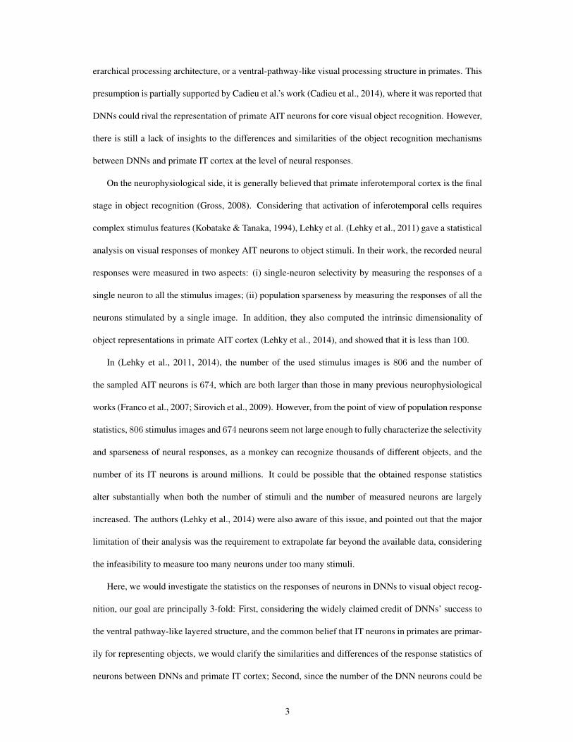
Figure 2: Probability density functions for high-selectivity and low-selectivity responses (Lehky et al.,

2011).

ness. Fig. 2 (from (Lehky et al., 2011)) shows an example of selectivity probability density functions,

where the high-selectivity probability density function (dashed line) has a heavier upper tail than the

low-selectivity probability density function (solid line).

2.3 Single-Neuron Selectivity, Population Sparseness, and Two Evaluation Crite-

ria

Single-neuron selectivity and population sparseness are two related characteristics to reflect the efficiency

and capacity of object representations in AIT cortex, which are extensively studied in many neurophysi-

ological works (Franco et al., 2007; Lehky et al., 2005, 2011). The single-neuron selectivity reflects the

response distributions of individual neurons to different stimuli, while the population sparseness reflects

the response distributions of all the neurons to a single image.

For the above mentioned 806 × 674 neural response matrix, each neuron has a fitted selectivity re-

sponse probability density function, and totally 674 such functions for all the 674 neurons are used to

evaluate the single-neuron selectivity. Similarly, each stimulus image has a population response proba-

bility density function, and totally 806 such functions for all the 806 stimulus images are used to evaluate

the population sparseness.

Given a probability density function for single-neuron responses (or population responses) as shown

in Fig. 2, if it has a substantial upper tail, it means high-selectivity responses have a larger probability

of occurrence at the extreme, in other words, the neuron is more selective (or the population response is

more sparse). Hence, the single-neuron selectivity (population sparseness) can be measured by “upper-

6

Figure 3: Architecture of VGG where the convolutional layer parameters are denoted as “〈Conv receptive

field size〉 - 〈number of channels〉”.

tail-heaviness” of the probability density function. In (Lehky et al., 2011), this upper-tail heaviness was

evaluated by two criteria, one is the kurtosis, and the other is the Pareto tail index. The kurtosis and the

Pareto tail index are discussed in Appendix A.

2.4 Intrinsic Dimensionality of Object Representations

Object representations in AIT neurons are largely redundant, it is speculated that some “intrinsic dimen-

sionality” exists for such representations (Lehky et al., 2014). Loosely speaking, among such redundant

representations, some “independent” representations should exist.

In (Lehky et al., 2014), Lehky et al. used both the Grassberger-Procaccia algorithm (Grassberger

et al., 1983) and a PCA(Principal Component Analysis)-based method to estimate the intrinsic dimen-

sionality of object representations, and found the PCA-based method is more stable. Hence, in this work,

we use only the PCA-based method to compute the intrinsic dimensionality of the object representations

of DNN neurons.

Broadly speaking, the intrinsic dimensionality computation by PCA is done in a 2-step manner.

Firstly, the intrinsic dimensionality of neuron responses under a fixed number of neurons and image

stimuli is computed by comparing the eigenvalue rankings of the original response matrix to their reshuf-

fled one, then the final intrinsic dimensionality is computed as the asymptotic one by extrapolation under

different combinations of image number and neuron number. The detailed PCA-based method for the

intrinsic dimensionality estimation is provided in Appendix B.

7

3 Response Statistics of DNN Neurons and Intrinsic Dimensional-

ity

The VGG network (Simonyan, 2014), a widely used deep neural network, is employed as our model

DNN. Then, the methods and criteria in Section 2 are used to evaluate the response statistics of DNN

neurons at different layers and the corresponding intrinsic dimensionality of object representations.

3.1 Datasets and VGG

We use the following two datasets as object stimuli in our experiments. The first one is the dataset used

in (Lehky et al., 2011, 2014), including 806 images as described in Section 2, denoted as Dataset I.

Since a small set of samples may miss rare large events, then underestimate single-neuron selectivity and

population sparseness of neural responses, a larger dataset – the validation set from the ImageNet dataset

– is also utilized, denoted as Dataset II. Dataset II includes 50000 images belonging to 1000 classes, 50

images per class. Several example images from this dataset are shown in Fig. 1(b). All the images in the

two datasets are resized to 224× 224 RGB images.

The VGG network, consisting of 16 convolutional layers with 3 × 3 convolution filters and 3 fully-

connected layers, was originally designed for object categorization. Its input is a fixed-size 224 × 224

RGB image, and its architecture is shown in Fig. 3. Considering that it is still pendent which layer in

a deep network acts similarly as primate IT cortex does, the statistics of the neural responses at the last

seven layers (including four convolutional layers and three fully-connected layers) in VGG are computed.

Note that the last layer of VGG outputs a probability vector of object category, and the other layers output

different features.

For notational convenience, the last seven layers are denoted as {L1, L2, L3, L4, L5, L6, L7} respec-

tively. As noted from Fig. 3, the {L1, L2, L3, L4} layers are the convolutional layers, each of which has

100352 = 14×14×512 neurons. The {L5, L6, L7} layers are the fully-connected layers. The {L5, L6}

layers have 4096 neurons respectively, and the L7 layer has 1000 neurons.

8

(a)

(b)

Figure 4: Single-neuron selectivity of neural responses at different layers of VGG to Dataset I and Dataset

II: (a) Selectivity for Dataset I; (b) Selectivity for Dataset II.

3.2 Neural Response Statistics by Kurtosis

3.2.1 Single-Neuron Selectivity

For each neuron at the last seven layers of VGG, the kurtosis of its responses to the 806 images in

Dataset I and the kurtosis of its responses to the 50000 images in Dataset II are computed respectively

for measuring the single-neuron selectivity, and the corresponding results are shown in Fig. 4. Since

9

normalization does not affect the single-neuron selectivity as discussed in Appendix A, we do not show

the computed kurtosis of the normalized responses.

As seen from Fig. 4, for the layers {L1, L2, L3, L4, L5, L6}, there exist a few neurons whose kurtosis

values are of one or two orders larger than median kurtosis value, indicating that these neurons are much

sensitive to a few special stimuli from the two datasets.

For the four convolutional layers {L1, L2, L3, L4} which have the same number of neurons, both the

computed mean and median kurtosis on Dataset I and Dataset II tend to become larger with the increase

of the layer number (although the mean and median kurtosis at Layer L2 are slightly larger than those at

Layer L3). This demonstrates that for different convolutional layers with the same number of neurons,

the probability distribution of the single-neuron responses of the neurons at a higher layer may have a

heavier upper tail than that at a lower layer.

For the fully-connected layers {L5, L6}, the computed mean and median kurtosis values on the two

datasets at Layer L5 are slightly smaller than those at Layer L6. Moreover, the computed mean and

median kurtosis values at the two fully-connected layers {L5, L6} are lower than or close to those at

the last convolutional layer L4 on the two datasets in most cases. This demonstrates that the probability

distribution of the single-neuron responses at the two fully-connected layers {L5, L6} has a lighter or

close upper tail than that at the last convolutional layer.

For the last fully-connected layer L7, the computed mean and median kurtosis values on Dataset II

are close to those on Dataset I, and they are lower than those at the other layers, which means most of the

neurons at this layer have weak selectivity. This is quite an expected result, because this layer outputs a

probability vector of object category, and it is not for object representation.

3.2.2 Population Sparseness

For each image in Dataset I and Dataset II, the kurtosis of the population responses at each layer is

computed for measuring the population sparseness, and the results are shown in Fig. 5(a) and Fig. 6(a).

In addition to the raw data, we also perform the sparseness calculation with the normalized data via Eq.

(A2) in Appendix A, and the kurtosis values for the normalized population responses are reported in Fig.

5(b) and Fig. 6(b).

10

(a)

(b)

Figure 5: Population sparseness of responses at different layers of VGG to Dataset I: (a) Sparseness for

the unnormalized data; (b) Sparseness for the normalized data.

Sparseness for the Unnormalized Data

As seen from Fig. 5(a) and Fig. 6(a), for the four convolutional layers {L1, L2, L3, L4}, the computed

mean and median kurtosis values on Dataset I and Dataset II tend to become larger with the increase of

the layer number (although the mean and median kurtosis at Layer L2 are slightly larger than those

at Layer L3), which is consistent with the hierarchical feature binding nature. This demonstrates that

11

(a)

(b)

Figure 6: Population sparseness at different layers of VGG to Dataset II: (a) Sparseness for the unnor-

malized data; (b) Sparseness for the normalized data.

for different convolutional layers with the same number of neurons, the probability distribution of the

population responses of the neurons at a higher layer has a heavier upper tail than that at a lower layer.

For the fully-connected layers {L5, L6}, the computed mean and median kurtosis values at Layer

L5 are slightly smaller than those at Layer L6. But, the computed mean and median kurtosis values at

Layers {L5, L6} are much lower than those at the last convolutional layer L4 on the two datasets. The

12

computed mean and median kurtosis values at Layer L7 are lower than those at the other layers in most

cases.

The above results seem to suggest that the DNN neurons at Layer L4 are responsible for object

representation. From LayerL4 to LayerL7, the object representations in the same category gradually lost

their individualism, and the prototypical categorization features are formed in a layer-by-layer fashion.

Sparseness for the Normalized Data

As seen from Fig. 5(a), Fig. 5(b), Fig. 6(a), and Fig. 6(b), the mean and median kurtosis values for the

normalized population responses are much larger than those for the unnormalized population responses,

mainly because some neural responses are amplified unusually when they are normalized with different

small mean responses respectively, due to the fact that for some images, many neurons are not responsive,

or of very weak response.

For the four convolutional layers {L1, L2, L3, L4}, the changing trend of the computed mean and

median kurtosis for the normalized data is similar to that for the unnormalized data, confirming once

again that for different convolutional layers with the same number of neurons, the population sparsity at

a higher layer is generally stronger than that at a lower layer.

For the fully-connected layers {L5, L6}, the computed mean and median kurtosis values for the

normalized data at Layer L5 are larger than those at Layer L6, but the computed mean and median

kurtosis values at these two layers are much lower than those at the last convolutional layerL4 on both the

two datasets. The computed mean and median kurtosis values for the normalized population responses at

Layer L7 are lower than those at the other layers in most cases. The above results are also consistent with

the categorization nature from Layer L4 to Layer L7 from the viewpoint of the population responses.

3.2.3 Variations of Response Statistics by Changing Neuron Numbers and Stimulus Numbers

Here, we calculate the single-neuron selectivity and the population sparseness of responses as the

dataset size increases by resampling subsets from Dataset II. Note that as done in (Lehky et al., 2011),

when dealing with the single-neuron responses, dataset size refers to the number of the stimulus images

tested on each neuron. When dealing with the population responses, dataset size refers to the number of

the DNN neurons in the population.

13

(a)

(b)

Figure 7: Mean kurtosis for both single-neuron responses and population responses with different image

samples and neurons at different layers of VGG: (a) For the unnormalized data; (b) For the normalized

data.

The image subset size of [100, 1000, 5000, 10000, 50000] is evaluated respectively. The neuron subset

sizes for each of the layers {L1, L2, L3, L4} are [100, 1000, 5000, 10000, 100000], the neuron subset

sizes for both the layers {L5, L6} are [100, 1000, 2000, 3000, 4000], and the neuron subset sizes for

Layer L7 are [100, 200, 300, 400, 1000]. Under each combination of the image number and the neuron

14

(a)

(b)

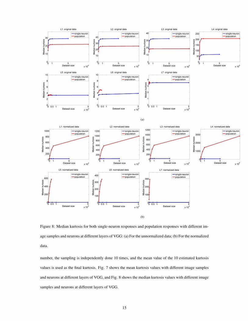
Figure 8: Median kurtosis for both single-neuron responses and population responses with different im-

age samples and neurons at different layers of VGG: (a) For the unnormalized data; (b) For the normalized

data.

number, the sampling is independently done 10 times, and the mean value of the 10 estimated kurtosis

values is used as the final kurtosis. Fig. 7 shows the mean kurtosis values with different image samples

and neurons at different layers of VGG, and Fig. 8 shows the median kurtosis values with different image

samples and neurons at different layers of VGG.

15

As is seen, both single-neuron selectivity and population sparseness behave in a monotonically non-

decreasing order as the size of the dataset increases. For the original unnormalized data, population

sparseness increases slower than single-neuron selectivity, but for the normalized data, population sparse-

ness increases faster than single-neuron selectivity. For the subsets of different sizes, the changing trends

of their computed mean kurtosis from Layer L1 to Layer L7 are similar, and the changing trends of their

computed median kurtosis from Layer L1 to Layer L7 are also similar.

3.3 Neural Response Statistics by Pareto Tail Index

At each of the last seven layers of DNNs, generalized Pareto distributions (GPDs) are fitted for both the

probability distribution function of single-neuron responses and the probability distribution function of

the population responses. Fig. 9 and Fig. 10 show the histograms of the computed Pareto tail index(i.e. k

in Eq. (A3) of Appendix A) for the single-neuron responses and the population responses to the stimulus

images from Dataset I. Fig. 11 and Fig. 12 show the histograms of the computed Pareto tail index for the

single-neuron responses and the population responses to the stimulus images from Dataset II.

3.3.1 Tail Index for Single-Neuron Responses

As seen from Fig. 9 and Fig. 11, for all the referred layers, the computed mean and median values of

k for the normalized single-neuron responses is quite close to those for the unnormalized single-neuron

responses.

For the four convolutional layers {L1, L2, L3, L4}, with the increase of the layer number, the mean

and median values of k on the two datasets tend to increase (although the mean and median values of k

for both the normalized/unnormalized data at Layer L2 is slightly larger than those at Layer L3), which is

consistent with the corresponding kurtosis results on the single-neuron responses in Section 3.2. For the

fully-connected layers {L5, L6}, the mean and median values of k for both the normalized/unnormalized

data at Layer L5 are slightly smaller than those at Layer L6. And the computed mean and median values

of k at {L5, L6} are lower than those at the last convolutional layer L4.

3.3.2 Tail Index for Population Responses

As seen from Fig. 10 and Fig. 12, for the four convolutional layers {L1, L2, L3, L4}, with the increase

16

(a)

(b)

Figure 9: Histograms of the computed Pareto tail indices of the single-neuron responses to Dataset I:(a)

For the unnormalized data; (b) For the normalized data.

of the layer number, the mean and median values of k for the population responses tend to become larger,

although the mean and median values of k at Layer L2 is slightly larger than those at Layer L3, which is

consistent with the above kurtosis results on the population responses.

For the fully-connected layers {L5, L6}, the mean and median values of k for the unnormalized data

at Layer L5 are slightly larger than those at Layer L6, which is inconsistent with the corresponding kurto-

17

(a)

(b)

Figure 10: Histograms of the computed Pareto tail indices of the population responses to Dataset I:(a)

For the unnormalized data; (b) For the normalized data.

sis results. The mean and median values of k for the normalized data at Layer L5 are also slightly larger

than those at Layer L6, which is consistent with the corresponding kurtosis results. The computed mean

and median values of k data at {L5, L6} are also lower than or close to those at the last convolutional

layer L4. In addition, the mean and median values of k at Layer L7 are close to or larger than those at the

other layers, which is not consistent with the corresponding kurtosis results on the population responses.

18

(a)

(b)

Figure 11: Histograms of the computed Pareto tail indices for the single-neuron responses to Dataset

II:(a) For the unnormalized data; (b) For the normalized data.

Moreover, for each referred layer, the mean and median values of k for the normalized popula-

tion responses are larger than those for the unnormalized population responses, which is consistent

with the corresponding kurtosis results. The mean value of k for the normalized/unnormalized popu-

lation responses to the two datasets is lower than that for the single-neuron responses at each of Layers

{L1, L2, L3, L4, L5, L6} in most cases. The mean value of k for the unnormalized population responses

19

(a)

(b)

Figure 12: Histograms of the computed Pareto tail indices for the population responses to Dataset II:(a)

For the unnormalized data; (b) For the normalized data.

to Dataset I at Layer L7 is also lower than that for the single-neuron responses, while the mean value of

k for the normalized/unnormalized population responses to Dataset II at Layer L7 is slightly larger than

that for the single-neuron responses.

20

3.4 DNN Neurons Versus AIT Neurons on Statistics of Responses

In (Lehky et al., 2011), kurtosis and tail index were used respectively to measure single-neuron selectiv-

ity and population sparseness of AIT neurons, the main results include: (i) For the unnormalized neural

responses, the population sparseness measured by kurtosis is greater than the single-neuron selectivity;

(ii) For the normalized neural responses, the population sparseness measured by kurtosis is also greater

than the single-neuron selectivity; (iii) The mean tail index for the unnormalized population responses is

greater than that for the unnormalized single-neuron responses; (iv) The mean tail index for normalized

population responses is greater than that for the normalized single-neuron responses; (v) The obser-

vations (i)–(iv) demonstrate that the estimated probability distributions for the single-neuron responses

in primate AIT cortex have lighter tailes, indicating that the critical features for individual neurons in

primate AIT cortex are not quite complex. In contrast, the estimated probability distributions for the

population responses have heavier tails, indicating that there is an indefinitely large number of different

critical features. These results are inconsistent with the traditional structural model of object recognition

where a small number of standard features is used.

In comparison, three main points are revealed in our above experimental results:

(1) It is observed that (i) For the unnormalized responses of DNN neurons at each of the last seven

layers, the population sparseness measured by kurtosis is smaller than the single-neuron selectivity in

most cases; (ii) For the normalized responses of DNN neurons at each of the last seven layers, the popu-

lation sparseness measured by kurtosis is much greater than the single-neuron selectivity in most cases;

(iii) The mean tail index for the unnormalized population responses is smaller than that for the unnor-

malized single-neuron responses in most cases; (iv) The mean tail index for the normalized population

responses is also smaller than that for the normalized single-neuron responses in most cases. Comparing

these results with the results of AIT neurons in (Lehky et al., 2011), except for the population sparse-

ness and the single-neuron selectivity measured by kurtosis for the normalized data, the conclusions on

the population sparseness versus the single-neuron selectivity for AIT neurons in (Lehky et al., 2011)

are in direct conflict to those of DNN neurons in this work, that is to say, the population sparseness is,

in contrast, smaller than the corresponding single-neuron selectivity for DNN neurons. This means the

DNN neurons are quite selective, and the population responses of DNN neurons are not as sparse as

21

those by AIT neurons, indicating that the object representation of DNN neurons is fundamentally dif-

ferent from that of AIT neurons in monkey. Considering the ubiquitous cross-talks between the ventral

and dorsal pathways, substantial feedbacks from higher visual areas to lower ones, and omnipresence of

horizontal inhibitions, the discrepancy of object representations between the AIT and DNN neurons is

not surprising. However, such direct conflicting results revealed in this work are nevertheless unexpected.

For the kurtosis measure for the normalized responses of DNN neurons, the single-neuron selectivity

is smaller than the population sparseness, which is consistent with the AIT neurons, but contrary to

the results measured by Pareto tail index for both the normalized and unnormalized data as well as the

results by kurtosis for the unnormalized data. The possible reason of this discrepancy could be 2-fold: At

first, due to the 4-degree computational nature of kurtosis as defined in (A1) of Appendix A, it is rather

sensitive to noise. We suspect this discrepancy is caused by noise; Secondly, the kurtosis is a global

measure of the probability density function (PDF) of neuron responses, it is possible in theory for a given

set of neural responses, the reached conclusion by kurtosis is different from that by Pareto tail index.

Since the Pareto tail index is designed specifically for measuring the tail heaviness of PDFs, we thought

the results by tail index are more trustworthy for comparison to the results in (Lehky et al., 2011).

(2) Our results show that the statistics of the neural responses at the convolutional layers are largely

different from those at the fully connected layers. When the convolutional layer number increases, both

the kurtosis and tail index measures of single-neuron selectivity and population sparseness for the un-

normalized/normalized responses increase, indicating that with the increase of the convolutional layer

number, the critical feature for individual neurons in DNNs would become more complex, and there

would be more features tuned by different neurons. This appears a typical hierarchical feature binding

process. The kurtosis and tail index measures of single-neuron selectivity and population sparseness at

the last convolutional layer are also larger than those at the fully-connected layers in most cases. There-

fore, the responses at the last convolutional layer can be considered as the object representation. From

then on, the fully connected layers are mainly engaged in learning a relatively smaller set of prototypical

features for object categorization, and the final one is the categorization output. We thought a good ob-

ject representation should at least satisfy the following two purposes: First for object identification which

needs to discriminate subtle differences from each other; second for object categorization which removes

22

the individualism within the same category, hence the significant differences between the convolutional

layers and the fully-connected layers revealed in this work are insightful and reasonable. For example, in

the HMAX model (Riesenhuber & Poggio, 1999), the categorization and object recognition submodels

share the same input, or the same output of object representation.

(3) With the increase of the image number, it is noted from Fig. 7 and Fig. 8: (i) The estimated

kurtosis for the single-neuron responses at each referred layer increases smoothly when the image number

is lower than 1000, and these results are consistent with those in AIT neurons (Lehky et al., 2011) where

806 images are used as the stimuli to AIT neurons. (ii) When the image number is large than 10000, the

estimated kurtosis for the single-neuron responses at the convolutional layers reaches a stable value, and

those at the fully-connected layers(except Layer L7) increase fast. These results are not consistent with

those in AIT neurons (Lehky et al., 2011), and they might indicate that the statistics of single-neuron

responses in IT cortex based on only 806 images cannot adequately characterize their single-neuron

selectivity. To reach a stable result, more images (in our case, larger than 10000 at least) are necessary.

When the neuron number increases, it is found from Fig. 7 and Fig. 8: (i) The estimated kurtosis

for the unnormalized population responses at each referred layer increases smoothly, and approximately

reaches a stable value. The results with the neuron number lower than 1000 are consistent with those in

AIT neurons (Lehky et al., 2011) where the responses of 674 neurons are recorded; (ii) The estimated

kurtosis for the normalized population responses at each referred layer increases, and their increase de-

celerates with the increase of the neuron number. These results are inconsistent with those in AIT neurons

where the increase of the mean kurtosis for the normalized population responses of AIT neurons is ac-

celerated when the neuron number increases from 4 to 650. This might indicate that the statistics of

neural responses in IT cortex based on only less than 1000 neurons cannot adequately characterize their

population sparseness. To reach a stable result, more neurons (in our case about 10000) are necessary.

3.5 Intrinsic Dimensionality

3.5.1 Calculating Intrinsic Dimensionality by the PCA-based Method

According to the discussions in Section 3.4, the features learnt from the last convolutional layer L4

of VGG are more appropriate for object representations, and the features learnt from the first two fully-

23

connected layers are used for object categorization. Hence in this section, the intrinsic dimensionality

of the outputted object features at the layers {L4, L5, L6} of VGG are computed by the PCA-based

estimation method, in order to further investigate the characteristics of object representation of neural

responses in DNNs.

Fig. 13 shows three example results on estimating the intrinsic dimensionality of the object repre-

sentation of neurons at the three layers with the stimulus images from Dataset I, where the red curve

represents the rank-ordered eigenvalues of the original responses, and the blue curve represents the rank-

ordered eigenvalues of randomly reshuffled responses. The intersection point of the two curves in each

subfigure is the estimated dimensionality {159, 62, 50} for Layers {L4, L5, L6} respectively. In addi-

tion, the first two principal components of the corresponding response matrix for Layer L4 accounts for

9% of the variance, lower than 17% for the inferotemporal responses to Dataset I (Lehky et al., 2014), and

15% for the inferotemporal responses obtained in (Baldassi et al., 2013), probably because the number

of neurons at Layer L4 is much larger than those in (Lehky et al., 2014) and (Baldassi et al., 2013). The

first two principal components of the corresponding response matrices for Layers {L5, L6} respectively

account for {22%, 29%} of the variance. This suggests that with the increase of the fully-connected layer

number, the learnt features become more prototypical for categorization.

Theoretically, the intrinsic dimensionality should be independent of the dataset size as well as the

number of the recorded neurons. However, in practice, any estimation depends on the used dataset size

and the number of the recorded neurons. To address this problem, as done in (Lehky et al., 2014), we

also compute the intrinsic dimensionality over a two-dimensional grid using neuron subsets of different

sizes and image subsets of different sizes. The dimensionality, as a function of the image number and the

neuron number, can be plotted as a surface in a three-dimensional space.

When dealing with Dataset I, the number of images is sampled at increments of 20 as done in (Lehky

et al., 2014), i.e. the image subset sizes are [20, 40, 60, ..., 800]. Considering that the number of neurons

at Layer L4 is much larger than those at Layers L5 and L4, the number of neurons at Layer L4 is sampled

at increments of 1000, while the number of neurons at Layer {L5, L6} is sampled at increments of 20

respectively.

When dealing with Dataset II, we compute the intrinsic dimensionality with the number of the neu-

24

(a) (b) (c)

Figure 13: Examples on estimating intrinsic dimensionality with the responses at Layers {L4, L5, L6}

for Dataset I.

(a) (b) (c)

(d) (e) (f)

Figure 14: Dimensionality surfaces corresponding to Layers {L4, L5, L6}: (a)(b)(c) Estimated dimen-

sionality surfaces using the images from Dataset I; (d)(e)(f) Estimated dimensionality surfaces using the

images from Dataset II.

rons not more than 4000 at Layer L4, since the occupied memories by the PCA-based method would

exceed the hardware configuration in our PC if all the images and all the neurons are considered. The

number of neurons at the three layers is sampled at increments of 100, and the number of images is

sampled at increments of 1000. Under each different combination of the image number and the neuron

number, the sampling is independently done 10 times, and the mean value of the 10 estimated intrinsic

25

dimensionality values is used as the final intrinsic dimensionality. Note that there exist a few neurons

which do not respond to any stimuli in our experiments, and they are simply removed before performing

the PCA-based method.

Figs. 14(a), 14(b), 14(c) show the dimensionality surfaces corresponding to Layers {L4, L5, L6}

respectively on Dataset I, and Figs. 14(d), 14(e), 14(f) show the dimensionality surfaces corresponding to

Layers {L4, L5, L6} respectively on Dataset II. As seen from these figures, when the number of neurons

and the number of images become large, the dimensionality surfaces vary smoothly in most cases.

The two-step procedure for estimating the asymptotic dimensionality in Appendix B is implemented

on Dataset I and Dataset II respectively. There exist two fitting orders for computing the asymptotic

dimensionality based on the one-dimensional asymptotic function (A4) in Appendix B: (I) “neuron →

image order”: Firstly fitting along the number of neurons and then along the number of images; (II)

“image→ neuron order”: Firstly fitting along the number of images and then along the number of neu-

rons. Both the two fitting orders are tested here, and Table 1 lists the corresponding results on Dataset

I and Dataset II. As seen from this table, different layers in VGG have different asymptotic dimension-

alities. The higher a layer is, the smaller its asymptotic dimensionality is in most cases, which implies

the representation is more category-prototypical. The asymptotic dimensionality for Dataset II at each

referred layer is larger than that for Dataset I, mainly because Dataset II is much larger than Dataset I.

These results confirm the existence of intrinsic dimensionality of object representation around the order

of hundred in (Lehky et al., 2014).

3.5.2 DNN Neurons Versus AIT Neurons on Intrinsic Dimensionality

In (Lehky et al., 2014), it was concluded: (i) The intrinsic dimensionality of object representations in

primate AIT cortex was around 100; (ii) The asymptotic approximation process seems not quite stable

due to the limited number of data.

Our results show that, for both the small-sized Dataset I and the large-sized Dataset II, the estimated

dimensionality values by using the responses of Layers {L4, L5, L6} of VGG all tend to reach asymptotic

limits, which supports the assumption that the intrinsic dimensionality of object representation in primate

AIT cortex reaches an asymptotic limit as both the number of stimulus images and the number of neurons

26

Table 1: Estimated asymptotic dimensionality values in both the monkey inferotemporal cortex and the

VGG network.

Layer Fit orderDimensionality

Dataset I Dataset II

Monkey inferotemporal cortex neuron → image 87 –

Monkey inferotemporal cortex image → neuron 105 –

VGG-L4 neuron → image 234 1504

VGG-L4 image → neuron 284 1569

VGG-L5 neuron → image 75 357

VGG-L5 image → neuron 102 336

VGG-L6 neuron → image 55 125

VGG-L6 image → neuron 74 117

approach to the infinity (Lehky et al., 2014).

In addition, it is noted from Table 1 that for each referred layer of VGG, the estimated dimensionality

on Dataset II is larger than the estimated dimensionality on Dataset I as well as the estimated dimen-

sionality (around 100) of object representation in primate IT cortex. It demonstrates that the estimated

asymptotic dimensionality is fairly sensitive to the size of the testing dataset. Hence, a sufficiently large

dataset should be used for reliably estimating the asymptotic dimensionality of object representations in

both DNNs and primate AIT cortex. Furthermore, the estimated dimensionality on Dataset I at Layer

L4 for object representation is much larger than that in primate IT cortex, indicating that the estimated

dimensionality in AIT cortex based on only less than 1000 neurons might not adequately reflect the in-

trinsic dimension of the object representation space, and a sufficiently large number of sample neurons

are necessary.

4 Conclusion

In this work, using the the concepts of single-neuron selectivity, population sparseness, and intrinsic

dimensionality as introduced in (Lehky et al., 2011, 2014) for IT neural responses in monkey, the statistics

of neural responses in DNNs are computed, and here are some concluding points:

27

• The response statistics of the neurons at later layers of DNNs are not fully consistent with those of

AIT neurons in monkey. DNN neurons are more selective, and their population responses are not

as sparse as AIT neurons in monkey.

• The changing trend of the response statistics from the low convolutional layers to the high fully-

connected layers suggests that DNNs are able to firstly learn a large set of complex features for

object representations through multiple convolutional layers, then learn a relatively small set of

prototypical features for categorization through the fully-connected layers, which could be the

reason of why DNNs perform well on visual object categorization. In addition, we thought object

representation and categorization representation are two very different issues, which should be

distinguished.

• The response statistics of DNN neurons with different combinations of the neuron number and

the stimulus number might suggest that, the statistics of AIT neural responses with only several

hundreds of neurons and stimulus images might not be sufficient. This is because the statistics of

DNN neural responses do not become stable until both the DNN neuron number and the image

number reach a sufficiently large value (in our case, at least large than 10000), although they are

similar to those of AIT neurons when both the DNN neuron number and the image number are

lower than 1000.

• The distribution of the intrinsic dimensionality of object representations in DNNs provides a sup-

port for the rationality that there exists an intrinsic dimensionality of object representation in pri-

mate AIT cortex (Lehky et al., 2014). However, a sufficiently large dataset and a sufficiently large

number of sampled neurons should be used for reliably estimating the asymptotic dimensionality

of object representations in both DNNs and primate AIT cortex.

• IT neurons in primate are for both object representation and object categorization. Object recogni-

tion requires distinguishing subtle differences among objects, while object categorization requires

removing differences within the same categorization. Hence, we thought the object representation

neurons should locate anatomically anterior to those for object recognition and categorization. We

even wonder whether the AIT neurons recorded in (Lehky et al., 2011) are truly for object repre-

28

sentations, not for object recognition or categorization, an issue might be worth further elucidating

in the future.

In sum, we seem the first to give a comparison on the response statistics of DNN neurons with respect

to those of AIT neurons in monkey. The results could be of reference for both those people working on

the object recognition in primate and in DNNs.

Acknowledgements

This work was supported by the Strategic Priority Research Program of the Chinese Academy of Sciences

(XDB02070002). The authors would like to thank Dr. Roozbeh Kiani for his provided data.

Appendix A: Kurtosis and Pareto Tail Index

Kurtosis: Kurtosis (strictly speaking, excess kurtosis) is a measure of the “peakedness” of a probability

distribution for both single-neuron selectivity and population sparseness in many existing works (Lehky

et al., 2005, 2007, 2011; Tolhurst et al., 2009). It only depends on the shape of the distribution, and is

independent of the mean or the variance. Kurtosis is defined as:

Kurt =1N

∑Ni=1 (ri − r̄)4

[ 1N

∑Ni=1 (ri − r̄)2]2

− 3 (A1)

where for single-neuron responses, ri is the response of a neuron to the i-th image, N is the number of

images; for population responses, ri is the response of the i-th neuron to an image, N is the number of

neurons. r̄ = 1N

∑Ni=1 ri is the mean response.

In addition, neurons in a population may have different activation levels in some cases, then high

population sparseness could arise as an artifact. To alleviate this problem, the normalized data rni , which

is obtained by dividing the response of each neuron by its mean response across all the stimulus images,

is also used for calculating kurtosis on both single-neuron selectivity and population sparseness:

rni =rir̄

(A2)

where ri is the response of a neuron to the i-th image, r̄ = 1N

∑Ni=1 ri is the mean response across all

29

N images. According to (A1) and (A2), the normalization has no effect on single-neuron selectivity in

principle, but does have an effect on population sparseness.

Pareto Tail Index: The Pareto tail index (Pickands, 1975) is utilized to analyse large responses occur-

ring on the upper tails of the probability density functions (PDFs). In (Lehky et al., 2011), tail data were

fitted with a generalized Pareto distribution by maximum likelihood.

The PDF for the generalized Pareto distribution is defined as:

p = f(r|k, σ, θ) =1

θ(1 + k

r − θσ

)−1− 1k (A3)

where σ is the scale, θ is the threshold where the upper tail of the probability density function starts, and

k is a shape parameter quantifying heaviness of the tail, called the tail parameter.

Generally speaking, if the kurtosis is large, it means the density function most probably has a heavy

tail. Similarly, if the tail index is large, the density function also has a heavy tail. Since population

sparseness and single-neuron selectivity are evaluated by the same criteria and computed by the same

formulae, from the computational point of view, they are of no difference.

Appendix B: PCA-based Method for Intrinsic Dimensionality Esti-

mation

In (Lehky et al., 2014), based on the recorded neural responses to a set of stimulus images, the PCA-based

method computed the intrinsic dimensionality of object representations by the following two steps:

(1) Different subsets with different combinations of the image number and the neuron number were

sampled from the original dataset. For each subset with a given number of neurons and images as well

as a randomly reshuffled version of it, PCA was performed on them respectively. Each set of eigenvalues

was normalized to sum to 1, and was sorted in a descending manner respectively. The eigenvalues of the

original data which were larger than those of the corresponding reshuffled data were considered to reflect

the signals in the original data, while the rest were considered noise. The number of the large eigenvalues

of reflecting the signals was considered as the intrinsic dimensionality of the original data. The authors

30

(Lehky et al., 2014) observed that for a given set of data, only one reshuffling was sufficient, and there

was little change in the intrinsic dimensionality estimation for repeated reshufflings.

(2) Assuming that the intrinsic dimensionality reached an asymptotic limit as both the image num-

ber and the neuron number approached to infinity, an asymptotic dimensionality was computed with

the obtained dimensionality values on different subsets as the final dimensionality. The asymptotic di-

mensionality was calculated in a two-step process: a one-dimensional asymptotic function was firstly fit

along one parameter (either number of neurons or number of images), then by fixing the first parameter

estimation, the asymptotic approximation along the other parameter was carried out. Lehky et al. (Lehky

et al., 2014) used two curve-fitting functions respectively for estimating asymptotic dimensionality, and

found that the estimated dimensionality values by the two functions were quite close. Hence, we only

use the following fitting function (the function (2.4) in (Lehky et al., 2014)) for estimating the asymptotic

dimensionality here:

z = a[1− (b

exp(xc

d )− 1 + b)e]f (A4)

where z was the dimensionality, x was the number of images or neurons, and {a, b, c, d, e, f} were fitting

parameters.

Noting that all nonlinear curve-fitting algorithms were dependent on parameter initials, it was hard to

give an appropriate set of initials for (A4) manually. Hence, each curve was repeatedly fit by trial-and-

error setting of initial parameters until the fitting error was lower than a predefined threshold ε.

References

Baldassi, C., Alemi-Neissi, A., Pagan, M., Dicarlo, J. J., Zecchina, R., Zoccolan, D. (2013). Shape

similarity, better than semantic membership, accounts for the structure of visual object representations

in a population of monkey inferotemporal neurons. PLoS Computational Biology, 9, e1003167.

Brosch, T., Tam, R. (2016). Efficient Training of Convolutional Deep Belief Networks in the Frequency

Domain for Application to High-Resolution 2D and 3D Images. Neural Computation, 27(1), 211–227.

Cadieu C., Hong H., Yamins D., Pinto N., Ardila D., Solomon E., et al. (2014) Deep Neural Networks

31

Rival the Representation of Primate IT Cortex for Core Visual Object Recognition. PLoS Comput Biol,

10(12), e1003963. doi:10.1371/journal.pcbi.1003963.

Franco L, Rolls ET, Aggelopoulos NC, Jerez JM.(2007) Neuronal selectivity, population sparseness, and

ergodicity in the inferior temporal visual cortex. Biol Cybern, 96, 547–560.

Girshick, R.(2015). Fast R-CNN. In Proc. ICCV, 1440–1448.

Grassberger, P., Procaccia, I. (1983). Measuring the strangeness of strange attractors. Physica, 9D,

189–208.

Gross C.(2008) Single neuron studies of inferior temporal cortex. Neuropsychologia, 46, 841–852.

He K., Zhang X., Ren S., Sun J. (2015). Delving deep into rectifiers: Surpassing human-level perfor-

mance on imagenet classification. In Proc. ICCV.

He K., Zhang X., Ren S., Sun J. (2016). Deep Residual Learning for Image Recognition. In Proc. CVPR.

Hinton, G. E. and Salakhutdinov, R. R. (2006) Reducing the dimensionality of data with neural networks.

Science, 313(5786), 504–507.

Jain A., Zamir R., Savarese S., Saxena A. (2016). Structural-RNN: Deep Learning on Spatio-Temporal

Graphs. In Proc. CVPR.

Kobatake E. and Tanaka K.(1994) Neuronal selectivities to complex object features in the ventral visual

pathway of the macaque cerebral cortex J Neurophysiol, 71, 856–867.

Krizhevsky, A., Sutskever, I. and Hinton, G. E. (2012). ImageNet Classification with Deep Convolutional

Neural Networks. In Proc. Advances in Neural Information Processing 25.

LeCun, Y., Bengio, Y. and Hinton, G. E. (2015). Deep Learning. Nature, 521, 436–444.

Lehky S., Sejnowski T., Desimone R. (2005) Selectivity and sparseness in the responses of striate com-

plex cells. Vision Research, 45, 57–73.

Lehky S., Sereno A. (2007) Comparison of shape encoding in primate dorsal and ventral visual pathways.

J Neurophysiol, 97, 307–319.

32

Lehky S., Kiani R., Esteky H., Tanaka K. (2011) Statistics of visual responses in primate inferotemporal

cortex to object stimuli. Journal of Neurophysiology, 106(3), 1097–1117.

Lehky S., Kiani R., Esteky H., Tanaka K. (2014) Dimensionality of Object Representations in Monkey

Inferotemporal Cortex. Neural Computation, 26, 2135–2162.

Long, J., Shelhamer, E., Darrell, T. (2015). Fully convolutional networks for semantic segmentation. In

Proc. CVPR, 3431–3440.

Martinez, W. L., Martinez, A. R., Solka, J. L. (2012). Exploratory data analysis with Matlab (2nd ed.)

Boca Raton, FL: CRC Press.

Pickands J. (1975). Statistical inference using extreme order statistics. Ann Stat, 3, 119–131.

Riesenhuber, M., Poggio, T. (1999). Hierarchical models of object recognition in cortex. Nature Neuro-

science, 2, 1019–1025.

Simonyan K., Zisserman A. (2014). Very Deep Convolutional Networks for Large-Scale Image Recog-

nition. arXiv preprint, arXiv:1409.1556.

Sirovich, L., Meytlis, M. (2009). Symmetry, probability, and recognition in face space. Proceedings of

the National Academy of Sciences of the United States of America, 106, 6895–6899.

Szegedy C., Liu W., Jia Y., et al. (2015). Going deeper with convolutions. In Proc. CVPR, 1–9.

Taigman, Y., Yang, M., Ranzato, M. A., Wolf, L. (2014). Deepface: Closing the gap to human-level

performance in face verification. In Proc. CVPR.

Tolhurst D., Smyth D., Thompson I. (2009) The sparseness of neuronal responses in ferret primary visual

cortex. J Neurosci, 29, 2355–2370.

Tygert, M., Bruna, J., Chintala, S., LeCun, Y., Piantino, S., Szlam A. (2016). A Mathematical Motivation

for Complex-Valued Convolutional Networks. Neural Computation, 28(5), 815–825.

Zhang, T., Dong, Q., Hu, Z. (2016). Pursuing Face Identity from View-Specific Representation to View-

Invariant Representation. In Proc. ICIP.

33