Embed Size (px)
Citation preview
University of Vermont University of Vermont
UVM ScholarWorks UVM ScholarWorks
Graduate College Dissertations and Theses Dissertations and Theses
2021
Statistics Of Particle Diffusion Subject To Oscillatory Flow In A Statistics Of Particle Diffusion Subject To Oscillatory Flow In A
Porous Bed Porous Bed
Kelly Curran University of Vermont
Follow this and additional works at: https://scholarworks.uvm.edu/graddis
Part of the Thermodynamics Commons
Recommended Citation Recommended Citation Curran, Kelly, "Statistics Of Particle Diffusion Subject To Oscillatory Flow In A Porous Bed" (2021). Graduate College Dissertations and Theses. 1439. https://scholarworks.uvm.edu/graddis/1439
This Thesis is brought to you for free and open access by the Dissertations and Theses at UVM ScholarWorks. It has been accepted for inclusion in Graduate College Dissertations and Theses by an authorized administrator of UVM ScholarWorks. For more information, please contact [email protected].
i
STATISTICS OF PARTICLE DIFFUSION
SUBJECT TO OSCILLATORY FLOW IN A
POROUS BED
A Thesis Presented
by
Kelly Curran
to
The Faculty of the Graduate College
of
The University of Vermont
In Partial Fulfillment of the Requirements
for the Degree of Master of Science
Specializing in Mechanical Engineering
August, 2021
Defense Date: July 16, 2021
Thesis Examination Committee:
Jeffrey S. Marshall, Ph.D., Advisor
George F. Pinder, PhD., Chairperson
William F. Louisos, Ph.D.
Cynthia J. Forehand, Ph.D., Dean of the Graduate College
i
ABSTRACT
Enhanced diffusion of a suspended particle in a porous medium has been observed when
an oscillatory forcing has been imposed. The mechanism of enhancement, termed
oscillatory diffusion, occurs when oscillating particles occasionally become temporarily
trapped in the pore spaces of the porous medium, and are then later released back into
the oscillatory flow. This thesis investigates the oscillatory diffusion process
experimentally, stochastically, and analytically. An experimental apparatus, consisting
of a packed bed of spheres subjected to an oscillatory flow field, was used to study the
dynamics of a single particle. A variety of statistical measures were used and developed
to characterize the diffusive process. A stochastic model was developed and showed great
agreement with the experimental results. The experimentally validated stochastic model
was then compared to an analytic prediction for diffusion coefficient from the
continuous-time random walk (CTRW) theory for a range of physical and numerical
parameter values. Good agreement between the stochastic model and CTRW theory was
observed for certain ranges of parameter values, while differences of predictions are
discussed and explained in terms of the assumptions used in each model. Results of the
paper are relevant to applications such as nanoparticle penetration into biofilms, drug
capsule penetration into human tissue, and microplastic transport within saturated soil.
ii
TABLE OF CONTENTS
LIST OF TABLES ............................................................................................................. iv
LIST OF FIGURES ............................................................................................................ v
CHAPTER 1: MOTIVATION AND OBJECTIVE ............................................................ 1
1.1. Motivation ....................................................................................................... 1
1.1.1 Biofilms....................................................................................................... 3
1.1.2 Targeted Drug Delivery .............................................................................. 7
1.1.3 Other Applications ...................................................................................... 9
1.2 Objective and Scope ......................................................................................... 10
CHAPTER 2: LITERACTURE REVIEW ....................................................................... 11
2.1 Particle Hindering Mechanisms ......................................................................... 11
2.1.1 Mechanical Filtration .................................................................................... 11
2.1.2 Straining ........................................................................................................ 14
2.1.3 Hydrodynamic Hindering ............................................................................. 15
2.1.4 Adhesive Capture .......................................................................................... 17
2.2 Hindered Diffusion in Biofilms ......................................................................... 20
2.2.1 Mechanical Filtration in Biofilms ................................................................. 20
2.2.2 Adhesive Effects in Biofilms ........................................................................ 22
2.3 Oscillatory Diffusion ......................................................................................... 23
2.3.1 Analytical Approximations ........................................................................... 23
2.3.1 Experimental Observations ........................................................................... 24
CHAPTER 3: EXPERIMENTAL METHOD .................................................................. 30
CHAPTER 4: DATA ANALYSIS ................................................................................... 36
CHAPTER 5: EXPERIMENTAL RESULTS .................................................................. 41
iii
5.1 Standard Statistical Measures ............................................................................ 41
5.2 Hold-up Measures .............................................................................................. 45
CHAPTER 6: STOCHASTIC MODEL ........................................................................... 53
CHAPTER 7: PARAMETRIC STUDY OF STOCHASTIC MODEL AND
COMPARISON TO CTRW THEORY ................................................................... 62
CHAPTER 8: CONCLUSIONS ....................................................................................... 74
REFERENCES ................................................................................................................. 78
iv
LIST OF TABLES
Table 1: Parameter values used for the different experimental runs. The uncertainty
is ±1 mm for oscillation amplitude, ± 0.03 mm for diameter of the small
particles, and ±0.1 mm for diameter of the large particles. The uncertainty for
frequency is 1% of the recorded value. ................................................................... 41 Table 2: Data on frequency of particle hold-up and best-fit values of dimensionless
𝜇 and 𝜎 coefficients from a log-normal distribution to the cumulative
distribution function for particle hold-up time. ....................................................... 50 Table 3: Comparison of the mean and standard deviation of the predictions for
dimensionless diffusion coefficient from the stochastic model and the CTRW
theory for different number of iterations of the model. ........................................... 68
v
LIST OF FIGURES
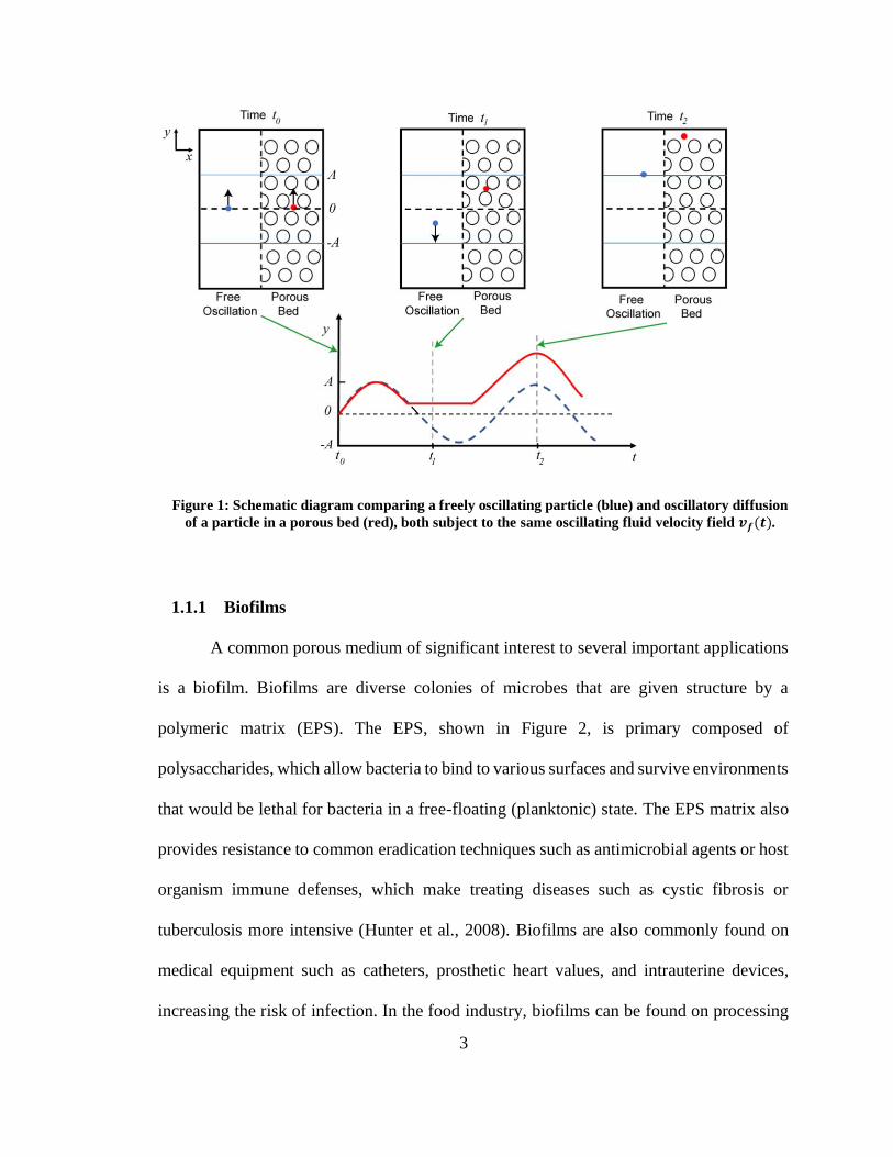
Figure 1: Schematic diagram comparing a freely oscillating particle (blue) and
oscillatory diffusion of a particle in a porous bed (red), both subject to the same
oscillating fluid velocity field 𝑣𝑓(𝑡). ......................................................................... 3
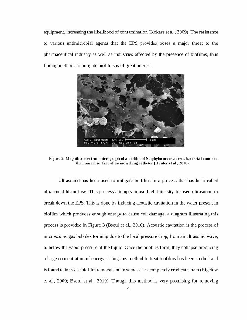
Figure 2: Magnified electron micrograph of a biofilm of Staphylococcus aureus
bacteria found on the luminal surface of an indwelling catheter (Hunter et al.,
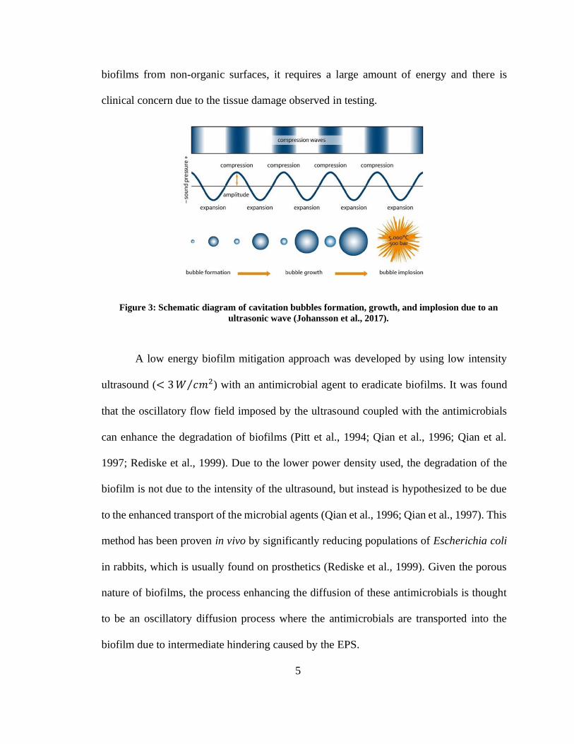
2008). ......................................................................................................................... 4 Figure 3: Schematic diagram of cavitation bubbles formation, growth, and implosion
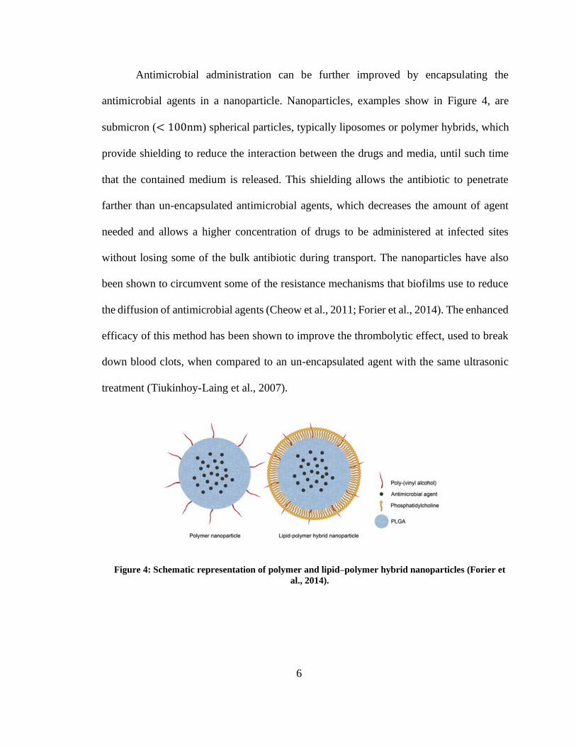
due to an ultrasonic wave (Johansson et al., 2017). .................................................. 5 Figure 4: Schematic representation of polymer and lipid–polymer hybrid
nanoparticles (Forier et al., 2014). ............................................................................ 6 Figure 5 Schematic of drug flow path through the human body after intravenous
injection. (Bertrand et al., 2011)................................................................................ 7 Figure 6 Schematic of nanoparticle (liposome) membrane rupturing by ultrasound
with (A) corresponding to a hydrophobic membrane while (B) corresponds to
a hydrophilic membrane (Schroeder et al., 2009). .................................................... 8 Figure 7: Illustration particle hindering by mechanical filtration with the black filled
circles representing the particles and the unfilled ovals represent the pores
(Kuzmina and Osipov, 2006). ................................................................................. 12 Figure 8: Cross section of pore, showing the equilateral triangle approximation used
to estimate the pore diameter (You et al., 2013). .................................................... 12 Figure 9: Composite image of the etched repeat pattern in a micromodel of sand,
measuring approximately 509 X 509 mm and etched to a depth of about 15
mm. Pore throats are on the order of 3–20 mm in diameter and the pores may
be up to 50 mm across. The pattern is repeated 100x100 times in the
micromodel, forming a square domain, with the inlet and outlet ports on each
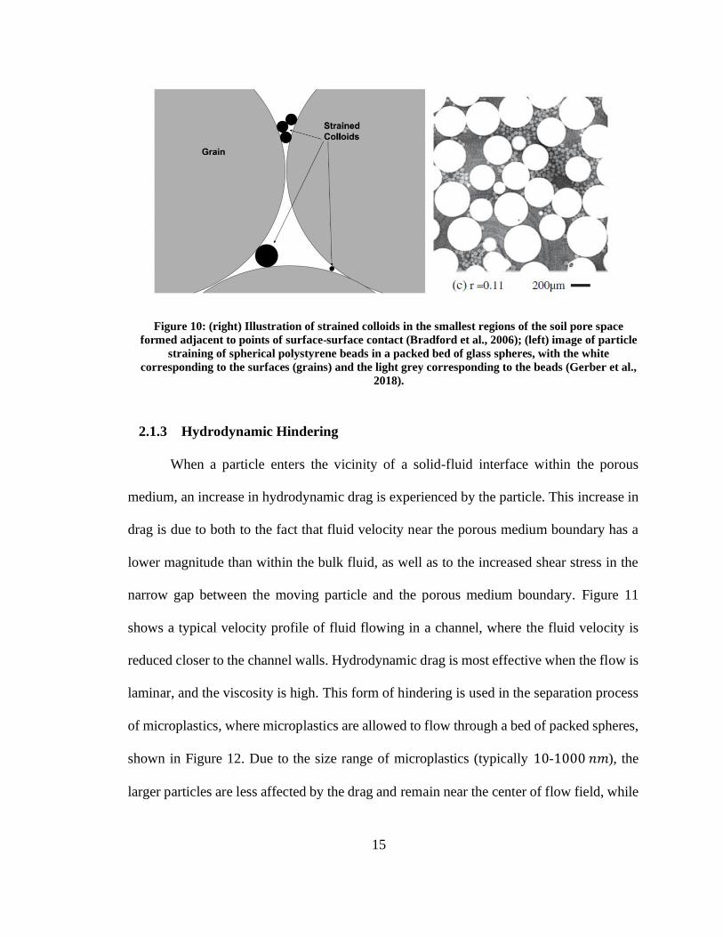
of the corners (Sirivithayapakorn and Keller, 2003). .............................................. 13 Figure 10: (right) Illustration of strained colloids in the smallest regions of the soil
pore space formed adjacent to points of grain-grain contact (Bradford et al.,
2006); (left) image of particle straining of spherical polystyrene beads in a
packed bed of glass spheres, with the white corresponding to the grains and the
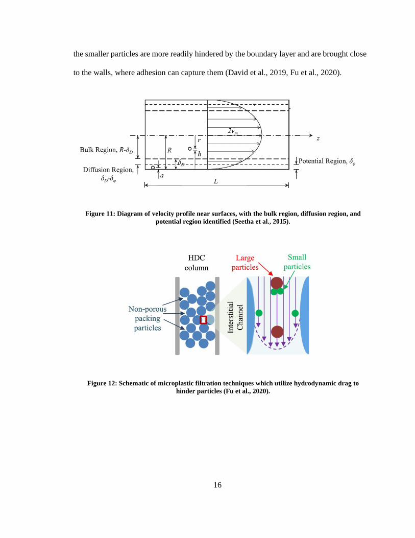
light grey corresponding to the beads (Gerber et al., 2018). ................................... 15 Figure 11: Diagram of velocity profile near surfaces, with the bulk region, diffusion
region, and potential region identified (Seetha et al., 2015). .................................. 16 Figure 12: Schematic of microplastic filtration techniques which utilize
hydrodynamic drag to hinder particles (Fu et al., 2020). ........................................ 16 Figure 13: Total particle-surface interaction energy plotted for (a) favorable
condition and (b) unfavorable condition. Adhesive forces are negative and
repulsive forces are positive (Kermani et al., 2020)................................................ 19 Figure 14: Typical repulsive, attractive, and net interaction energy curves between a
sphere and a flat plate based on DLVO theory for an unfavorable interaction
(Hahn et al., 2004). .................................................................................................. 19
vi
Figure 15: The variance for 3 diffusive processes; superdiffusion α = 1.5 (upper blue
curve), normal diffusion α = 1 (middle yellow curve), and subdiffusion α = 0.5
(lower green curve) (Oliveira et al., 2019). ............................................................. 22 Figure 16: Schematic of experimental apparatus consisting of an acoustic transducer
forcing injected tracer particles through a packed bed of spheres (Thomas and
Chrysikopoulos, 2007). ........................................................................................... 25 Figure 17: Schematic diagram of the experimental apparatus consisting of an
ultrasonic transducer forcing either a liposome or nanoparticle suspension
toward an alginate film (Ma et al., 2015). ............................................................... 27 Figure 19: Plot showing the fluorescent intensity with the depth into the hydrogel for
the ultrasound treated gel (Ma et al., 2015). ............................................................ 28 Figure 20: Comparison of predicted probability density functions (PDF) for the
stochastic model (symbols) and the one-dimensional diffusion equation (solid
line) are plotted. The PDF was capture at three time steps, 𝑡 = 2 (triangles),
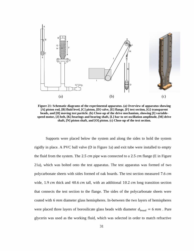
10 (crosses), and 100 (circles) (Marshal, 2016). ................................................... 29 Figure 21: Schematic diagrams of the experimental apparatus. (a) Overview of
apparatus showing [A] piston rod, [B] fluid level, [C] piston, [D] valve, [E]
flange, [F] test section, [G] transparent beads, and [H] moving test particle. (b)
Close-up of the drive mechanism, showing [I] variable-speed motor, [J] belt,
[K] bearings and bearing shaft, [L] bar to set oscillation amplitude, [M] drive
shaft, [N] piston shaft, and [O] piston. (c) Close-up of the test section. ................. 31 Figure 22: Plots illustrating statistical measures for a random walk process, showing
(a) the ensemble variance and (b) the ratio of the kurtosis over the variance
squared as functions of time, (c) autocorrelation as a function of time delay,
and (d) the power spectrum. Theoretical predictions are plotted as dashed lines.
................................................................................................................................. 39 Figure 24: Plots showing time variation of (a) mean (red) and variance (black) of y
position and (b) ratio 𝑦𝑘𝑢𝑟𝑡/𝑦𝑣𝑎𝑟2 for Case B-2. Theoretical results are
indicated by dashed lines. ........................................................................................ 43 Figure 25: Plots showing (a) the autocorrelation and (b) the power spectrum for Case
B-2. The dashed line in (a) is the theoretical expression in Eq. (15) for a
random-walk process, and the dashed line in (b) is for the theoretical power
law for random walk diffusion. ............................................................................... 43 Figure 26: Probability density function of velocity for Case B-2 at time 𝑓𝑜𝑠𝑐𝑡 = 0.4
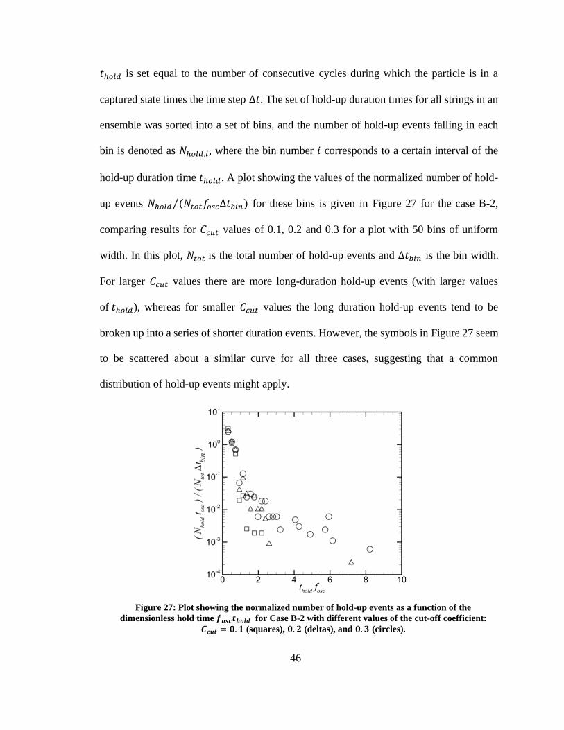
. The dashed line is for the Gaussian curve 𝑓(𝑥) = 0.5 𝑒𝑥𝑝(−𝑥2 ) . ..................... 45 Figure 27: Plot showing the normalized number of hold-up events as a function of
the dimensionless hold time 𝑓𝑜𝑠𝑐𝑡ℎ𝑜𝑙𝑑 for Case B-2 with different values of the
cut-off coefficient: 𝐶𝑐𝑢𝑡 = 0.1 (squares), 0.2 (deltas), and 0.3 (circles). .............. 46 Figure 28: Example comparing experimental data (symbols) and a log-normal fit
(solid line) for (a) the complementary cumulative distribution function (1-
C.D.F.) and (b) the probability density function (P.D.F.) for Case B-4. ................. 48 Figure 29: Comparison of complementary cumulative distribution function for cases
with particle diameters of 𝑑 = 0.52 mm (red squares, Case R-4) and 𝑑 = 1.3
mm (black deltas, Case B-4). .................................................................................. 51
vii
Figure 30: Comparison of complementary cumulative distribution function for cases
with (a) oscillation frequency of 𝑓𝑜𝑠𝑐 = 0.15 Hz (squares, Case B-1), 𝑓𝑜𝑠𝑐 =0.25 Hz (X's, Case B-2), 𝑓𝑜𝑠𝑐 = 0.50 Hz (circles, Case B-3), and 𝑓𝑜𝑠𝑐 =0.75 Hz (deltas, Case B-4) and (b) oscillation amplitude of 𝑦𝑎𝑚𝑝 = 15.3 mm
(squares, Case R-2), 𝑦𝑎𝑚𝑝 = 31.0 mm (deltas, Case R-5), and 𝑦𝑎𝑚𝑝 =
42.9 mm (circles, Case R-6).................................................................................... 52 Figure 31: Probability density function (P.D.F.) for the distribution of pore size
difference (𝑏 − 𝑏𝑚𝑖𝑛)/𝑑𝑏𝑒𝑎𝑑 with different values of the parameters 𝜇𝑝𝑜𝑟𝑒 and
𝜎𝑝𝑜𝑟𝑒: (a) distribution for 𝜎𝑝𝑜𝑟𝑒 = 1 and 𝜇𝑝𝑜𝑟𝑒 = −3 (A, blue), −2 (B, red),
0 (C, green) and (b) distribution for 𝜇𝑝𝑜𝑟𝑒 = −1.8 and 𝜎𝑝𝑜𝑟𝑒 = 0.5 (A, blue),
1.5 (B, red), 2.0 (C, green). The dashed black curve is the distribution used for
the example computation in the current paper (𝜇𝑝𝑜𝑟𝑒 = −1.8,𝜎𝑝𝑜𝑟𝑒 = 1.0). ......... 54
Figure 32: Flow chart of the stochastic model for a particle with diameter 𝑑. ................. 55 Figure 33: Plot showing time variation of a sample experimental trace for 𝑦𝑝(𝑡)
(bottom, left-hand axis) and 𝑣𝑝(𝑡) (top, right-hand axis) for the stochastic
model. ...................................................................................................................... 58 Figure 34: Illustration of the diffusive characteristic of the particle motion: (a) traces
of 20 particles released from 𝑦 = 0, (b) P.D.F. of particle location for 2000
traces sorted into 50 bins in 𝑦/𝐴, evaluated at time 𝑓𝑜𝑠𝑐𝑡 = 25. ............................ 58 Figure 35: Plots comparing a variety of statistical measures for the experimental case
B-2 (B-2, black line I plots a-c) and the stochastic model (SM, red line in plots
a-c): (a) the ensemble variance and (b) the ratio of the kurtosis over the
variance squared as functions of time; (c) autocorrelation as a function of time
delay, and (d) power spectrum for the stochastic model. Dashed lines indicate
(a) best fit to slope of variance passing through origin, (b) theoretical value for
a normally distributed process, and (d) 𝑓−2 power law typical of a random walk
process. .................................................................................................................... 60 Figure 36: Plot showing (a) the complementary cumulative distribution function (1-
C.D.F.) and (b) the probability density function (P.D.F.), with the stochastic
model prediction indicated by symbols and the log-normal fit for the
experimental data in Case B-2 indicated by solid lines........................................... 61 Figure 37: Plots showing results for particle capture-time distribution, including: (a)
the complementary cumulative distribution function C.C.D.F. and (b) the
probability density function (P.D.F.). The data (symbols) were computed from
the stochastic model for the example case described in Chapter 4. The least-
square fit (lines) were obtained using the exponential distribution in Eq. (9)
with 𝜏1 = 1.82. ........................................................................................................ 64 Figure 38: Plots showing results for free particle oscillation time distribution,
including: (a) the complementary cumulative distribution function C.C.D.F.
and (b) the probability density function (P.D.F.). The data (symbols) were
computed from the stochastic model for the example case described in Chapter
4. The least-square fit (lines) were obtained using the exponential distribution
in Eq. (9) with 𝜏0 = 1.44. ....................................................................................... 65
viii
Figure 39: Sensitivity study of the dimensionless diffusion coefficient predictions for
the stochastic model (red triangles) and the CTRW theory (black squares) as
functions of three different numerical parameters: (a) 𝐶𝑐𝑢𝑡, (b) Δ𝑡′, and (c) 𝐶ℎ.
Symbols represent the mean value and error bars represent the standard
deviation of 100 repeated computations for each point. ......................................... 70
1
CHAPTER 1: MOTIVATION AND OBJECTIVE
1.1. Motivation
The problem of diffusion of particles immersed in a porous medium is applicable
to many fields. Furthermore, it has been experimentally observed in a number of contexts
that imposing an oscillatory flow field (e.g., via an acoustic signal) on particles in a porous
medium has increased their effective diffusion coefficient, allowing the particles to
penetrate farther and faster than previously able (Ma et al., 2015; Paul et al., 2014). The
mechanism facilitating this enhanced diffusion has been identified as a form of bulk
diffusion termed oscillatory diffusion (Balakrishnan and Venkataraman, 1981b; Marshall,
2016).
Oscillatory diffusion occurs when a particle, in an oscillatory flow field,
experiences random hindering, due to interactions with the surrounding porous medium,
that either reduces the particle's velocity below that of the surrounding flow field or
completely stops the particle. This process, averaged over an ensemble of particles,
resembles a diffusion process (Marshall, 2016). A visual representation of this process is
shown in Fig 1.1, where two particle paths are shown with one particle freely oscillating
(blue) while the other particle experiences hindering due to a porous medium (red). Both
particles are subjected to the same oscillatory flow field (𝑣𝑓). The figure shows the particle
position as a time series, with arrows indicating the direction of the flow field. At the initial
time (t0), both particles start at the same y-position (y0), with velocity oriented in the
positive y-direction. Both particles oscillate in phase together until the red particle becomes
stuck in one of the pores at time t1. This hindering of the red particle causes the blue particle
to travel farther than the red particle during this time, resulting in an offset. Once the flow
2
field changes directions, the red particle is released and can now move with the flow field
in phase with the blue particle, but the offset in the y-direction remains. The corresponding
particle trajectories are also plotted in Figure 1, with the red line corresponding to the
hindered (red) particle and the blue dashed line corresponding to the freely oscillating
(blue) particle. It is observed that the process of the red particle being stuck for a period of
time and then re-entering the flow allows for it to travel further from the initial y-position
(𝑦0) than is the case for the blue particle, which simply oscillates up and down with the
flow field. As the process is repeated with increasing time, the hindered (red) particle can
drift further and further away from its initial position. Applying this process to a finite
number of particles leads to a bulk diffusion away from the initial particle location y0.
While the oscillatory diffusion phenomenon is qualitatively understood, an improved
quantitative understanding of the phenomenon would aid in development of methods that
utilize an oscillating flow field to enhance diffusion in porous media.
3
Figure 1: Schematic diagram comparing a freely oscillating particle (blue) and oscillatory diffusion
of a particle in a porous bed (red), both subject to the same oscillating fluid velocity field 𝒗𝒇(𝒕).
1.1.1 Biofilms
A common porous medium of significant interest to several important applications
is a biofilm. Biofilms are diverse colonies of microbes that are given structure by a
polymeric matrix (EPS). The EPS, shown in Figure 2, is primary composed of
polysaccharides, which allow bacteria to bind to various surfaces and survive environments
that would be lethal for bacteria in a free-floating (planktonic) state. The EPS matrix also
provides resistance to common eradication techniques such as antimicrobial agents or host
organism immune defenses, which make treating diseases such as cystic fibrosis or
tuberculosis more intensive (Hunter et al., 2008). Biofilms are also commonly found on
medical equipment such as catheters, prosthetic heart values, and intrauterine devices,
increasing the risk of infection. In the food industry, biofilms can be found on processing
4
equipment, increasing the likelihood of contamination (Kokare et al., 2009). The resistance
to various antimicrobial agents that the EPS provides poses a major threat to the
pharmaceutical industry as well as industries affected by the presence of biofilms, thus
finding methods to mitigate biofilms is of great interest.
Figure 2: Magnified electron micrograph of a biofilm of Staphylococcus aureus bacteria found on
the luminal surface of an indwelling catheter (Hunter et al., 2008).
Ultrasound has been used to mitigate biofilms in a process that has been called
ultrasound histotripsy. This process attempts to use high intensity focused ultrasound to
break down the EPS. This is done by inducing acoustic cavitation in the water present in
biofilm which produces enough energy to cause cell damage, a diagram illustrating this
process is provided in Figure 3 (Bsoul et al., 2010). Acoustic cavitation is the process of
microscopic gas bubbles forming due to the local pressure drop, from an ultrasonic wave,
to below the vapor pressure of the liquid. Once the bubbles form, they collapse producing
a large concentration of energy. Using this method to treat biofilms has been studied and
is found to increase biofilm removal and in some cases completely eradicate them (Bigelow
et al., 2009; Bsoul et al., 2010). Though this method is very promising for removing
5
biofilms from non-organic surfaces, it requires a large amount of energy and there is
clinical concern due to the tissue damage observed in testing.
Figure 3: Schematic diagram of cavitation bubbles formation, growth, and implosion due to an
ultrasonic wave (Johansson et al., 2017).
A low energy biofilm mitigation approach was developed by using low intensity
ultrasound (< 3 𝑊 𝑐𝑚2⁄ ) with an antimicrobial agent to eradicate biofilms. It was found
that the oscillatory flow field imposed by the ultrasound coupled with the antimicrobials
can enhance the degradation of biofilms (Pitt et al., 1994; Qian et al., 1996; Qian et al.
1997; Rediske et al., 1999). Due to the lower power density used, the degradation of the
biofilm is not due to the intensity of the ultrasound, but instead is hypothesized to be due
to the enhanced transport of the microbial agents (Qian et al., 1996; Qian et al., 1997). This
method has been proven in vivo by significantly reducing populations of Escherichia coli
in rabbits, which is usually found on prosthetics (Rediske et al., 1999). Given the porous
nature of biofilms, the process enhancing the diffusion of these antimicrobials is thought
to be an oscillatory diffusion process where the antimicrobials are transported into the
biofilm due to intermediate hindering caused by the EPS.
6
Antimicrobial administration can be further improved by encapsulating the
antimicrobial agents in a nanoparticle. Nanoparticles, examples show in Figure 4, are
submicron (< 100nm) spherical particles, typically liposomes or polymer hybrids, which
provide shielding to reduce the interaction between the drugs and media, until such time
that the contained medium is released. This shielding allows the antibiotic to penetrate
farther than un-encapsulated antimicrobial agents, which decreases the amount of agent
needed and allows a higher concentration of drugs to be administered at infected sites
without losing some of the bulk antibiotic during transport. The nanoparticles have also
been shown to circumvent some of the resistance mechanisms that biofilms use to reduce
the diffusion of antimicrobial agents (Cheow et al., 2011; Forier et al., 2014). The enhanced
efficacy of this method has been shown to improve the thrombolytic effect, used to break
down blood clots, when compared to an un-encapsulated agent with the same ultrasonic
treatment (Tiukinhoy-Laing et al., 2007).
Figure 4: Schematic representation of polymer and lipid–polymer hybrid nanoparticles (Forier et
al., 2014).
7
1.1.2 Targeted Drug Delivery
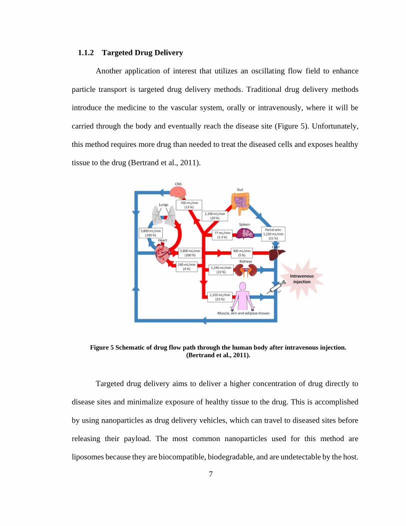
Another application of interest that utilizes an oscillating flow field to enhance
particle transport is targeted drug delivery methods. Traditional drug delivery methods
introduce the medicine to the vascular system, orally or intravenously, where it will be
carried through the body and eventually reach the disease site (Figure 5). Unfortunately,
this method requires more drug than needed to treat the diseased cells and exposes healthy
tissue to the drug (Bertrand et al., 2011).
Figure 5 Schematic of drug flow path through the human body after intravenous injection.
(Bertrand et al., 2011).
Targeted drug delivery aims to deliver a higher concentration of drug directly to
disease sites and minimalize exposure of healthy tissue to the drug. This is accomplished
by using nanoparticles as drug delivery vehicles, which can travel to diseased sites before
releasing their payload. The most common nanoparticles used for this method are
liposomes because they are biocompatible, biodegradable, and are undetectable by the host.
8
Targeting can be done either passively or actively. Passive targeting utilizes the enhanced
permeability and retention (EPR) effect, which suggests that nanoparticles are more likely
to accumulate in diseased cells, while active targeting needs information about the diseased
cells so that compatible receptors can be added to the nanoparticle to promote bonding
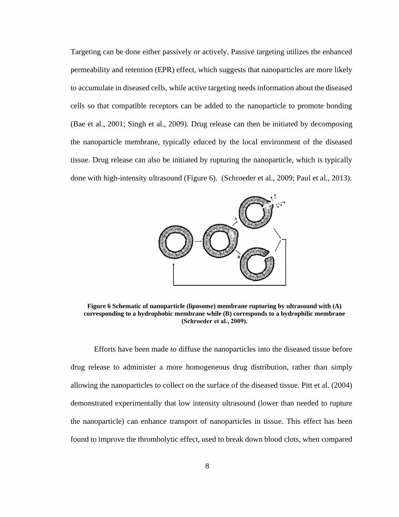
(Bae et al., 2001; Singh et al., 2009). Drug release can then be initiated by decomposing
the nanoparticle membrane, typically educed by the local environment of the diseased
tissue. Drug release can also be initiated by rupturing the nanoparticle, which is typically
done with high-intensity ultrasound (Figure 6). (Schroeder et al., 2009; Paul et al., 2013).
Figure 6 Schematic of nanoparticle (liposome) membrane rupturing by ultrasound with (A)
corresponding to a hydrophobic membrane while (B) corresponds to a hydrophilic membrane
(Schroeder et al., 2009).
Efforts have been made to diffuse the nanoparticles into the diseased tissue before
drug release to administer a more homogeneous drug distribution, rather than simply
allowing the nanoparticles to collect on the surface of the diseased tissue. Pitt et al. (2004)
demonstrated experimentally that low intensity ultrasound (lower than needed to rupture
the nanoparticle) can enhance transport of nanoparticles in tissue. This effect has been
found to improve the thrombolytic effect, used to break down blood clots, when compared
9
to an un-encapsulated agent with the same ultrasonic treatment (Tiukinhoy-Laing et al.,
2007).
1.1.3 Other Applications
There are a variety of other applications involving particle transport in porous
media of various types, for which particle diffusion plays an important role. While
oscillatory diffusion has not been employed in these applications to date, the potential
exists that application of an oscillatory flow field (such as an acoustic field) could also be
beneficial in enhancing particle diffusion in such applications. One such application of
particular interest is the removal of microplastic particles from soil. Microplastics (MPs)
are very small plastic particles (< 5mm) that are generated by processes such as plastics
manufacturing, sewage treatment, and agricultural systems (Corradini et al., 2019; Fu et
al., 2020). These MP’s typically end up in marine environments, but they have more
recently been identified as a major environmental issue in terrestrial soil (Huffer et al.,
2019). The issue with MPs in soil is that their size allows them to be consumed by soil
dwelling organisms, which can have a negative impact on agricultural production and has
the potential to introduce plastic into the food chain (Rillig et al., 2012, Rillig et al., 2017).
The presence of MPs have also been found to effect organisms that play an important role
in modifying the soil system (Kim et al., 2019, Souza Machado et al., 2019). A large effort
is put on accurately and effectively extracting microplastics from samples for study (Wang
et al., 2018; Fu et al., 2020). Development of techniques for effective removal of
microplastics from soil is an on-going challenge, but oscillatory diffusion might prove to
be a useful method to enhance transport of microplastics out of a layer of soil.
10
1.2 Objective and Scope
The objective of this thesis is to provide a fundamental quantitative understanding
of oscillatory diffusion by studying the individual dynamics of a particle in a packed bed
of spheres subjected to an oscillatory flow field. An experiment in which a series of tests
observing individual particle motion subject to oscillatory flow has been conducted, in
which the particle diameter and the frequency and amplitude of the oscillatory flow are
varied. A statistical analysis of the particle response to the oscillatory flow was conducted,
describing both the freely oscillating motion of the particle and the period of particle
hindering by the surrounding porous bed. The results from the experiment were used to
improve and validate a stochastic model and to validate a previously developed continuous
time random walk (CTRW) theory for oscillatory diffusion (Balakrishnan and
Venkataraman, 1981b).
A literature review related to hindered diffusion and oscillatory diffusion of
particles in porous media is provided in Chapter 2. The experimental apparatus and
methods are explained in Chapter 3. The statistical measures used for data analysis are
presented in Chapter 4. The experimental results are discussed in Chapter 5. A stochastic
model of oscillatory diffusion is introduced in Chapter 6. A parametric study comparing
parameter sensitivities for both the stochastic model as well as the CTRW theory is
presented and discussed in Chapter 7. Conclusions are provided in Chapter 8.
11
CHAPTER 2: LITERACTURE REVIEW
2.1 Particle Hindering Mechanisms
Oscillatory diffusion relies heavily on the ability of the surrounding porous media
to suppress or hinder the motion of the diffusing particles. It is, therefore, important to
understand the various hindering mechanisms that come into play for porous media of
different types. Hindered diffusion occurs when a diffusing particle is slowed down as it
approaches the surface of the porous medium in which it is embedded. This hindering of
the particle motion can occur via a variety of different forces imposed on the diffusing
particle by the fluid and/or directly by the surrounding porous medium, including
hydrodynamic drag, friction, van der Waals adhesion, electrostatic interactions, etc. The
influence of this local forcing causes the particles diffusion rate to be reduced or
temporarily stopped. Hindered diffusion is commonly observed in systems involving
porous media diffusion of colloidal particles, such as microplastics in soil or passive
particle filtration processes.
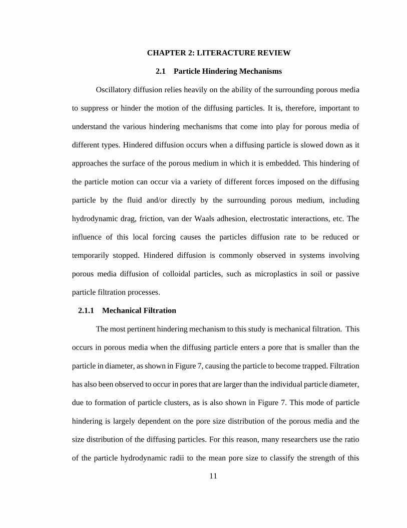
2.1.1 Mechanical Filtration
The most pertinent hindering mechanism to this study is mechanical filtration. This
occurs in porous media when the diffusing particle enters a pore that is smaller than the
particle in diameter, as shown in Figure 7, causing the particle to become trapped. Filtration
has also been observed to occur in pores that are larger than the individual particle diameter,
due to formation of particle clusters, as is also shown in Figure 7. This mode of particle
hindering is largely dependent on the pore size distribution of the porous media and the
size distribution of the diffusing particles. For this reason, many researchers use the ratio
of the particle hydrodynamic radii to the mean pore size to classify the strength of this
12
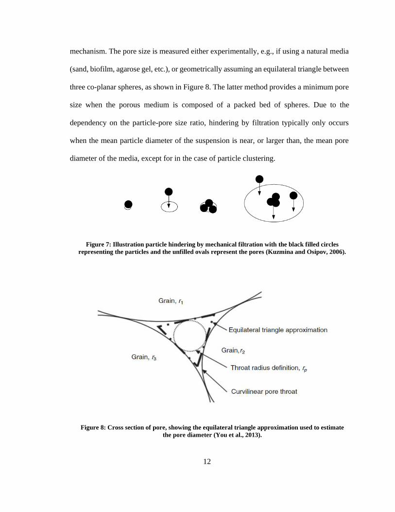
mechanism. The pore size is measured either experimentally, e.g., if using a natural media
(sand, biofilm, agarose gel, etc.), or geometrically assuming an equilateral triangle between
three co-planar spheres, as shown in Figure 8. The latter method provides a minimum pore
size when the porous medium is composed of a packed bed of spheres. Due to the
dependency on the particle-pore size ratio, hindering by filtration typically only occurs
when the mean particle diameter of the suspension is near, or larger than, the mean pore
diameter of the media, except for in the case of particle clustering.
Figure 7: Illustration particle hindering by mechanical filtration with the black filled circles
representing the particles and the unfilled ovals represent the pores (Kuzmina and Osipov, 2006).
Figure 8: Cross section of pore, showing the equilateral triangle approximation used to estimate
the pore diameter (You et al., 2013).
13
The particle-pore diameter ratio has been shown to help classify different regimes
of behavior for particle in porous media. Gerber et al. (2018) examined the transport of
spherical polystyrene beads in a packed bed of glass spheres and found that adjusting the
particle-pore ratio not only determined when the particles would begin to be trapped in the
pores, but also determined the transition to formation of particle caking, a critical issue in
water reclamation systems (Wang et al., 2018) where the particles can no longer penetrate
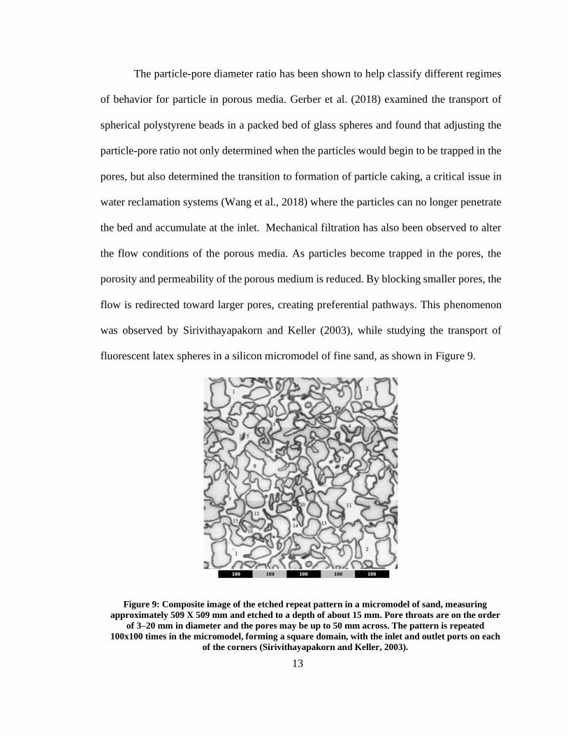
the bed and accumulate at the inlet. Mechanical filtration has also been observed to alter
the flow conditions of the porous media. As particles become trapped in the pores, the
porosity and permeability of the porous medium is reduced. By blocking smaller pores, the
flow is redirected toward larger pores, creating preferential pathways. This phenomenon
was observed by Sirivithayapakorn and Keller (2003), while studying the transport of
fluorescent latex spheres in a silicon micromodel of fine sand, as shown in Figure 9.
Figure 9: Composite image of the etched repeat pattern in a micromodel of sand, measuring
approximately 509 X 509 mm and etched to a depth of about 15 mm. Pore throats are on the order
of 3–20 mm in diameter and the pores may be up to 50 mm across. The pattern is repeated
100x100 times in the micromodel, forming a square domain, with the inlet and outlet ports on each
of the corners (Sirivithayapakorn and Keller, 2003).
14
2.1.2 Straining
Another important hindering mechanism is straining, which can be thought of as a
combination of mechanical filtration and adhesive capture (Bradford et al., 2002; Bradford
et al., 2003; Bradford et al., 2006; Cu et al., 2006; Porubcan et al., 2011). In this process,
particles enter the smallest region of a pore space at a surface-surface contact where they
become trapped, as shown in Figure 10 (Bradford et al., 2006). This entrapment is due to
frictional forces between the particles and surfaces as well as attracting adhesive forces
between the particle surface and the surface of the porous medium. This form of hindering
has been shown to be important in filtration systems of colloidal particles in porous media.
Straining has been suggested to improve agreement between the established theory
describing colloidal hindering, known as Clean Bed Filtration Theory (CBFT), and
experimental observations. Including straining as a deposition mechanism has been found
to reduce error between experimental data and models significantly (Bradford 2003). Like
mechanical filtration, the effects of straining are estimated by the ratio of particle to pore
size, where straining is most likely to occur in cases where this ratio is very small.
15
Figure 10: (right) Illustration of strained colloids in the smallest regions of the soil pore space
formed adjacent to points of surface-surface contact (Bradford et al., 2006); (left) image of particle
straining of spherical polystyrene beads in a packed bed of glass spheres, with the white
corresponding to the surfaces (grains) and the light grey corresponding to the beads (Gerber et al.,
2018).
2.1.3 Hydrodynamic Hindering
When a particle enters the vicinity of a solid-fluid interface within the porous
medium, an increase in hydrodynamic drag is experienced by the particle. This increase in
drag is due to both to the fact that fluid velocity near the porous medium boundary has a
lower magnitude than within the bulk fluid, as well as to the increased shear stress in the
narrow gap between the moving particle and the porous medium boundary. Figure 11
shows a typical velocity profile of fluid flowing in a channel, where the fluid velocity is
reduced closer to the channel walls. Hydrodynamic drag is most effective when the flow is
laminar, and the viscosity is high. This form of hindering is used in the separation process
of microplastics, where microplastics are allowed to flow through a bed of packed spheres,
shown in Figure 12. Due to the size range of microplastics (typically 10-1000 𝑛𝑚), the
larger particles are less affected by the drag and remain near the center of flow field, while
16
the smaller particles are more readily hindered by the boundary layer and are brought close
to the walls, where adhesion can capture them (David et al., 2019, Fu et al., 2020).
Figure 11: Diagram of velocity profile near surfaces, with the bulk region, diffusion region, and
potential region identified (Seetha et al., 2015).
Figure 12: Schematic of microplastic filtration techniques which utilize hydrodynamic drag to
hinder particles (Fu et al., 2020).
17
2.1.4 Adhesive Capture
A major hindering mechanism for low velocity flows with small particles is
adhesive capture. Adhesion can occur from van der Waals force (due to dipole interactions)
as well as by electrostatic forces between the particle and porous media surfaces. The
theory formulated to describe these surface-surface interactions in an ionic liquid is known
as Derjaguin–Landau–Verwey–Overbeek (DLVO) theory. The electric double layer (EDL)
is formed when ions within the liquid are attracted to the surface of a charged body. These
ions tend to form in layers, with the first layer (the surface charge) consisting of ions of the
opposite charge as the body which are adsorbed onto the body surface and the second layer
(the diffuse layer) consisting of ions of the same charge as the body which are attracted to
the ions in the first layer. The effect of these two layers is to electrically screen the body
charge. When two charged bodies come sufficiently close to each other (typically on the
order of tens of nanometers), the EDLs of the bodies can overlap giving rise to an
electrostatic force between the bodies. DLVO theory combines this electrostatic force with
the attractive van der Waals force to examine the net force acting between the two bodies.
If the charges of the interacting bodies (e.g., a diffusing particle and a porous
medium surface) are the opposite, the electrostatic force from the overlapping EDLs is
attractive and the interaction is said to be favorable. In this case, the colloidal particles
quickly deposit on the surface of the porous medium. If the charge of the two interacting
bodies are the same, the electrostatic force from the overlapping EDLs is repulsive and the
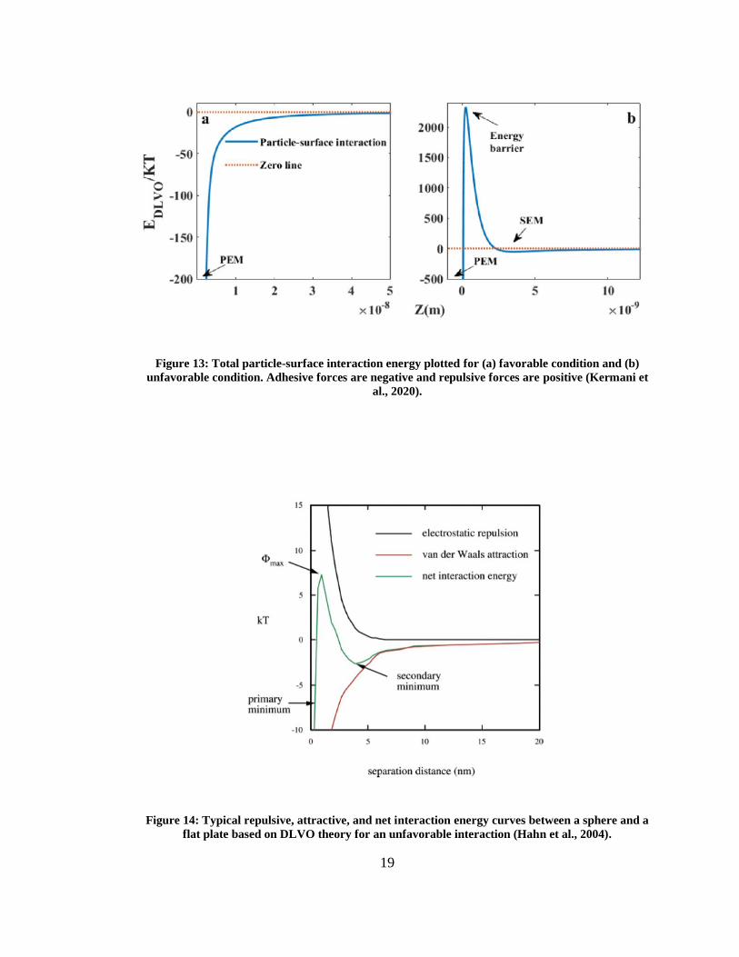
interaction is said to be unfavorable (Lee, 1991; Pizzi and Mittal, 2003). Plots of the total
interaction energy help to explain how and where particle adhesion to the porous medium
can occur. Figure 2.7 shows the total interaction energy for cases where the wall and
18
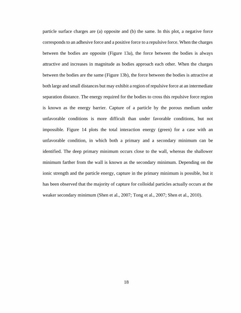
particle surface charges are (a) opposite and (b) the same. In this plot, a negative force
corresponds to an adhesive force and a positive force to a repulsive force. When the charges
between the bodies are opposite (Figure 13a), the force between the bodies is always
attractive and increases in magnitude as bodies approach each other. When the charges
between the bodies are the same (Figure 13b), the force between the bodies is attractive at
both large and small distances but may exhibit a region of repulsive force at an intermediate
separation distance. The energy required for the bodies to cross this repulsive force region
is known as the energy barrier. Capture of a particle by the porous medium under
unfavorable conditions is more difficult than under favorable conditions, but not
impossible. Figure 14 plots the total interaction energy (green) for a case with an
unfavorable condition, in which both a primary and a secondary minimum can be
identified. The deep primary minimum occurs close to the wall, whereas the shallower
minimum farther from the wall is known as the secondary minimum. Depending on the
ionic strength and the particle energy, capture in the primary minimum is possible, but it
has been observed that the majority of capture for colloidal particles actually occurs at the
weaker secondary minimum (Shen et al., 2007; Tong et al., 2007; Shen et al., 2010).
19
Figure 13: Total particle-surface interaction energy plotted for (a) favorable condition and (b)
unfavorable condition. Adhesive forces are negative and repulsive forces are positive (Kermani et
al., 2020).
Figure 14: Typical repulsive, attractive, and net interaction energy curves between a sphere and a
flat plate based on DLVO theory for an unfavorable interaction (Hahn et al., 2004).
20
2.2 Hindered Diffusion in Biofilms
The previous section discussed several hindering mechanisms that are present in a
large variety of physical systems and processes. To give some prospective on how these
mechanisms operate in a specific real-world system, hindered particle diffusion in biofilms
is examined in the current section. A biofilm is considered a porous medium due to the
surrounding hydrogel formed of the extracellular polymeric substance (EPS) (Miller et al.,
2013; Laspidou et al., 2014). Due to the high density of the EPS, flow is restricted through
the pores, which are typically on the order of < 100𝑛𝑚 (Stewart et al., 2003). This
restrictive flow environment means that transport is dominated by diffusion. Biofilms
typically have a large water content, in some cases up to 90%, so the diffusion of water
(𝐷𝑤) is typically the reference point when comparing biofilm diffusion. The ratio of the
diffusion coefficient within the biofilm (𝐷𝑏) over that in water is called the relative
diffusion coefficient (𝐷𝑏 𝐷𝑤⁄ ). The presence of the polymer matrix in the biofilm has been
observed to reduce the diffusion coefficient resulting in a relative diffusion coefficient that
is less than unity (Beuling et al., 1998). Several mechanisms have been investigated to
understand the hindering effects of a biofilm, most notably mechanical filtration and
adhesion. Reaction-diffusion will not be discussed in this review, but it can also be a
significant factor for determining penetration depth for reactive substances (Stewart et al.,
2003).
2.2.1 Mechanical Filtration in Biofilms
Mechanical filtration is an important hindering mechanism for biofilms. As is
typical for a system experiencing mechanical filtration, the particle-pore size ratio plays an
important role. The value of this ratio has been studied for several different biofilms and
21
hydrogel models. Fatin-Rouge et al. (2004) found the critical particle-pore ratio of an
agarose gel to be near 0.4, where for values below this ratio anomalous diffusion was
observed and for values above this ratio mechanical filtration was observed. Anomalous
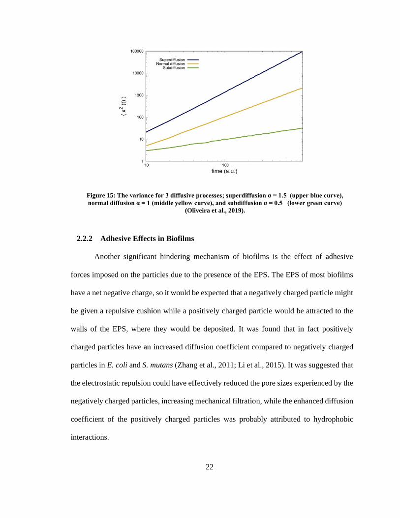
diffusion refers to diffusion in which the variance does not increase linearly in time, and is
typical of Brownian motion in inhomogeneous porous media (Oliveira et al., 2019). Figure
15 shows the two regions of anomalous diffusion, either superdiffusive or subdiffusive,
where the particle diffusion rate is either increasing exponentially with time (α > 1) or
decaying exponentially with time (α < 1) respectively. The variance is typically fit with
an exponential as shown in (1),
𝐥𝐨𝐠𝒏→∞⟨𝒓𝟐(𝒕)⟩~𝒕𝜶 (1)
The exponent (α) is used to classify whether or not a diffusive process is anomalous.
The prediction of anomalous diffusion in biofilms and hydrogels was confirmed by
Peulen et al. (2011), who found the diffusion coefficient value for P. fluorescens to
decrease exponentially with distance into the biofilm, though the anomalous coefficients
that were extracted are close to unity, . 89 < α < 1.01. The prediction of mechanical
filtration for particle-pore ratios less than 0.4 was further probed using a range of particle
sizes, 40-550 𝑛𝑚 (Forier et al., 2014a). It was found that the particle size cutoff was around
100-130 𝑛𝑚 for B. multivorans and P. aeruginosa, with particles above this threshold
showing almost no penetration into the biofilm.
22
Figure 15: The variance for 3 diffusive processes; superdiffusion α = 1.5 (upper blue curve),
normal diffusion α = 1 (middle yellow curve), and subdiffusion α = 0.5 (lower green curve)
(Oliveira et al., 2019).
2.2.2 Adhesive Effects in Biofilms
Another significant hindering mechanism of biofilms is the effect of adhesive
forces imposed on the particles due to the presence of the EPS. The EPS of most biofilms
have a net negative charge, so it would be expected that a negatively charged particle might
be given a repulsive cushion while a positively charged particle would be attracted to the
walls of the EPS, where they would be deposited. It was found that in fact positively
charged particles have an increased diffusion coefficient compared to negatively charged
particles in E. coli and S. mutans (Zhang et al., 2011; Li et al., 2015). It was suggested that
the electrostatic repulsion could have effectively reduced the pore sizes experienced by the
negatively charged particles, increasing mechanical filtration, while the enhanced diffusion
coefficient of the positively charged particles was probably attributed to hydrophobic
interactions.
23
2.3 Oscillatory Diffusion
2.3.1 Analytical Approximations
One of the earliest studies of diffusion in an oscillatory potential was developed to
describe the dynamics of ions in superionic conductors. The process was made up of two
possible states, (1) short range Brownian diffusion and (2) free oscillation state. The
Brownian diffusion is described by the corresponding Langevin equation, given by
𝒎�̈� + 𝒎𝜸�̇� − 𝑲(𝒙) = 𝒇(𝒕) (2)
Here, 𝑚 corresponds to the particle mass, 𝑥 is the particles position, γ is the friction
coefficient, K(x) = -∂V(x)
∂x is the oscillatory forcing, where 𝑉(𝑥) is the potential field, and
f(t) is the stochastic force. Due to the random nature of Brownian particles, 𝑓(𝑡) is modeled
as Gaussian white noise with an autocorrelation function given by
⟨𝒇(𝒕)𝒇(𝟎)⟩ = 𝟐𝒎𝜸𝒌𝒃𝑻𝜹(𝒕) (3)
where kb is the Boltzmann Constant, T is the temperature, and δ(t) is delta
function. The two states are achieved by looking at the temperature extremes. If kbT ≪ V0,
then oscillation is dominant, and if kbT ≫ V0, Brownian diffusion is dominant. In-between
these limits, both Brownian diffusion and oscillation play a role (Dieterich and Peschel,
1977).
Another approach to describe the dynamics of oscillatory diffusion uses the Fokker-
Planck equation. This equation estimates the time evolution of the probability density
24
functions for stochastic differential equations. Unfortunately, it very difficult to find
closed-form analytical solutions to the general Fokker-Planck equation, though several
generalized versions have been developed such as the Smoluchowski equation, developed
for Brownian diffusion. Solutions to this equation have been found, such as the Hill
solution, but due to its assumption of a weak potential there is a limited range of angular
velocities and time that can be predicted accurately (Das, 1979).
Continuous time random walk (CTRW) is a generalized random walk theory which
treats the time in-between successive steps as a random variable. This theory has been
shown to successfully describe many different processes including anomalous diffusion,
photon imaging, and financial distributions (Sokolov and Klafter, 2007; Chernomordik et
al., 2010; Masoliver et al., 2006). CTRW has also been applied to oscillatory diffusion by
Balakrishnan and Venkataraman (1981). They use a two-state model, where the particle is
either in a ‘flight’ state when the particle is freely moving between sites or an oscillatory
state, when the particle experiences local oscillations at a single site. The time duration that
the particle occupies at each state is treated as a random variable, which is called the
'holding time'. Unlike the Langevin or Fokker-Planck methods, the CTRW theory is not
restricted to a single dimension and provides closed-form solutions for the diffusion
coefficient as well as a number of other parameters.
2.3.1 Experimental Observations
An experimental study examining the effect of an acoustic field on diffusion in a
packed bed of spherical beads was reported by Vogler and Chrysikopoulos (2001) for
solute diffusion and by Thomas and Chrysikopoulos (2007) for particle diffusion. Thomas
and Chrysikopoulos (2007) forced tracer particles through a wet bed of packed spheres
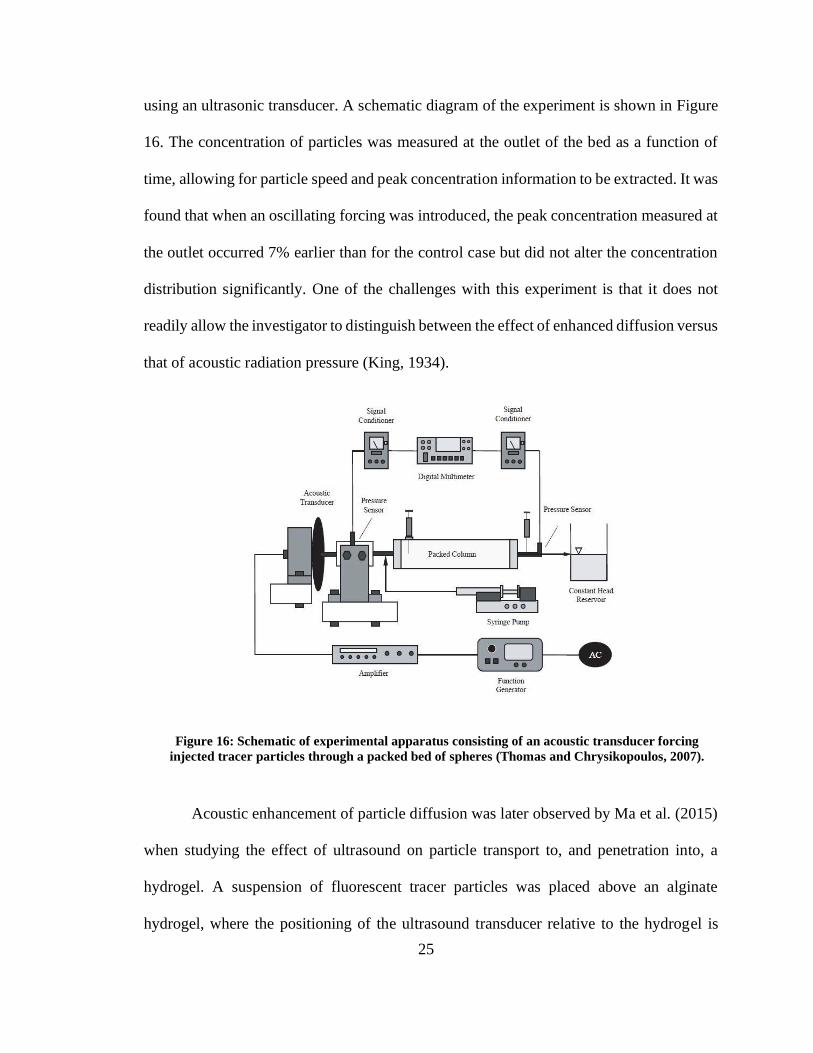
25
using an ultrasonic transducer. A schematic diagram of the experiment is shown in Figure
16. The concentration of particles was measured at the outlet of the bed as a function of
time, allowing for particle speed and peak concentration information to be extracted. It was
found that when an oscillating forcing was introduced, the peak concentration measured at
the outlet occurred 7% earlier than for the control case but did not alter the concentration
distribution significantly. One of the challenges with this experiment is that it does not
readily allow the investigator to distinguish between the effect of enhanced diffusion versus
that of acoustic radiation pressure (King, 1934).
Figure 16: Schematic of experimental apparatus consisting of an acoustic transducer forcing
injected tracer particles through a packed bed of spheres (Thomas and Chrysikopoulos, 2007).
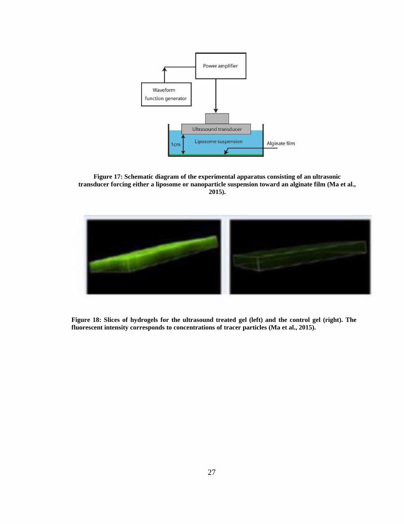
Acoustic enhancement of particle diffusion was later observed by Ma et al. (2015)
when studying the effect of ultrasound on particle transport to, and penetration into, a
hydrogel. A suspension of fluorescent tracer particles was placed above an alginate
hydrogel, where the positioning of the ultrasound transducer relative to the hydrogel is
26
indicated in the schematic diagram in Figure 17. The ultrasound was found to improve
transport to the gel surface due to the formation of an acoustic streaming flow. Ultrasound
was also observed to increase the penetration of nanoparticles into the hydrogel. Images of
a three-dimensional section of the hydrogels showing fluorescence induced by penetrated
nanoparticles is shown in Figure 18 for both the control case (with no ultrasound) and for
the case with ultrasound treatment. The fluorescent intensity corresponds to the
concentration of nanoparticles. The control case appears to have experienced almost no
penetration, while the ultrasound-treated case shows significant fluorescence, indicating
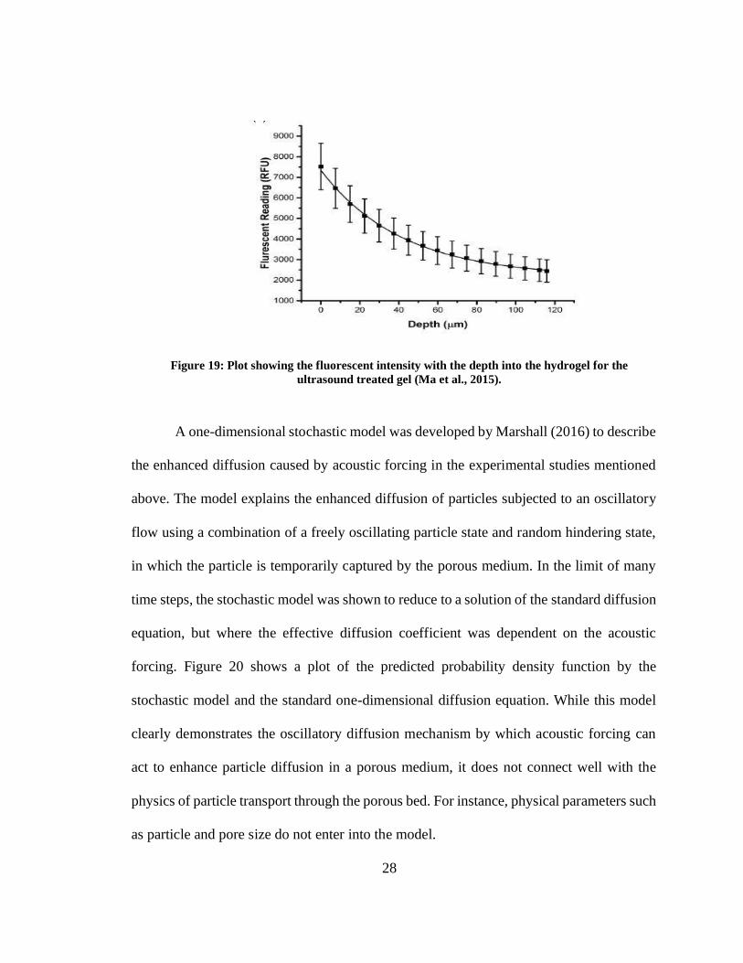
that a large number of nanoparticles have penetrated into the hydrogel to various depths.
The fluorescent intensity was measured as a function of depth, as shown in Figure 19,
where an exponential decay can be observed. In a follow up study, Ma et al. (2018)
obtained detailed measurements of the effect of ultrasound on the diffusion coefficient for
two sizes of nanoparticles (20 and 100nm) diffusing into an agarose hydrogel. The
apparatus is similar to the previous study, but now the hydrogel is formed of two layers,
one of which is seeded with fluorescent tracer particles and the other of which is unseeded.
The experiment measured the rate of diffusion of particles from the seeded layer into the
unseeded layer both with no acoustic forcing and in the presence of low-intensity
ultrasound forcing. An increase in diffusion coefficient of between 74-133% was
experienced with ultrasound compared to the control case (with no ultrasound).
27
Figure 17: Schematic diagram of the experimental apparatus consisting of an ultrasonic
transducer forcing either a liposome or nanoparticle suspension toward an alginate film (Ma et al.,
2015).
Figure 18: Slices of hydrogels for the ultrasound treated gel (left) and the control gel (right). The
fluorescent intensity corresponds to concentrations of tracer particles (Ma et al., 2015).
28
Figure 19: Plot showing the fluorescent intensity with the depth into the hydrogel for the
ultrasound treated gel (Ma et al., 2015).
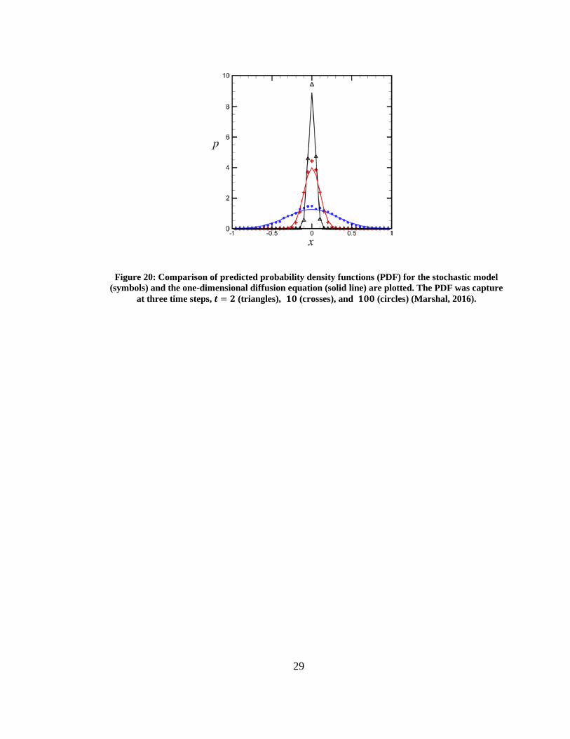
A one-dimensional stochastic model was developed by Marshall (2016) to describe
the enhanced diffusion caused by acoustic forcing in the experimental studies mentioned
above. The model explains the enhanced diffusion of particles subjected to an oscillatory
flow using a combination of a freely oscillating particle state and random hindering state,
in which the particle is temporarily captured by the porous medium. In the limit of many
time steps, the stochastic model was shown to reduce to a solution of the standard diffusion
equation, but where the effective diffusion coefficient was dependent on the acoustic
forcing. Figure 20 shows a plot of the predicted probability density function by the
stochastic model and the standard one-dimensional diffusion equation. While this model
clearly demonstrates the oscillatory diffusion mechanism by which acoustic forcing can
act to enhance particle diffusion in a porous medium, it does not connect well with the
physics of particle transport through the porous bed. For instance, physical parameters such
as particle and pore size do not enter into the model.
29
Figure 20: Comparison of predicted probability density functions (PDF) for the stochastic model
(symbols) and the one-dimensional diffusion equation (solid line) are plotted. The PDF was capture
at three time steps, 𝒕 = 𝟐 (triangles), 𝟏𝟎 (crosses), and 𝟏𝟎𝟎 (circles) (Marshal, 2016).
30
CHAPTER 3: EXPERIMENTAL METHOD
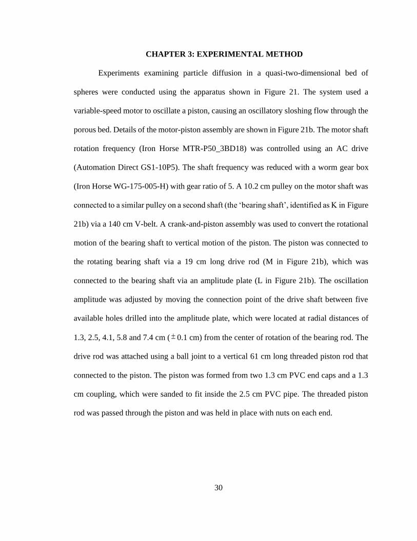
Experiments examining particle diffusion in a quasi-two-dimensional bed of
spheres were conducted using the apparatus shown in Figure 21. The system used a
variable-speed motor to oscillate a piston, causing an oscillatory sloshing flow through the
porous bed. Details of the motor-piston assembly are shown in Figure 21b. The motor shaft
rotation frequency (Iron Horse MTR-P50_3BD18) was controlled using an AC drive
(Automation Direct GS1-10P5). The shaft frequency was reduced with a worm gear box
(Iron Horse WG-175-005-H) with gear ratio of 5. A 10.2 cm pulley on the motor shaft was
connected to a similar pulley on a second shaft (the ‘bearing shaft’, identified as K in Figure
21b) via a 140 cm V-belt. A crank-and-piston assembly was used to convert the rotational
motion of the bearing shaft to vertical motion of the piston. The piston was connected to
the rotating bearing shaft via a 19 cm long drive rod (M in Figure 21b), which was
connected to the bearing shaft via an amplitude plate (L in Figure 21b). The oscillation
amplitude was adjusted by moving the connection point of the drive shaft between five
available holes drilled into the amplitude plate, which were located at radial distances of
1.3, 2.5, 4.1, 5.8 and 7.4 cm ( 0.1 cm) from the center of rotation of the bearing rod. The
drive rod was attached using a ball joint to a vertical 61 cm long threaded piston rod that
connected to the piston. The piston was formed from two 1.3 cm PVC end caps and a 1.3
cm coupling, which were sanded to fit inside the 2.5 cm PVC pipe. The threaded piston
rod was passed through the piston and was held in place with nuts on each end.
31
Figure 21: Schematic diagrams of the experimental apparatus. (a) Overview of apparatus showing
[A] piston rod, [B] fluid level, [C] piston, [D] valve, [E] flange, [F] test section, [G] transparent
beads, and [H] moving test particle. (b) Close-up of the drive mechanism, showing [I] variable-
speed motor, [J] belt, [K] bearings and bearing shaft, [L] bar to set oscillation amplitude, [M] drive
shaft, [N] piston shaft, and [O] piston. (c) Close-up of the test section.
Supports were placed below the system and along the sides to hold the system
rigidly in place. A PVC ball valve (D in Figure 1a) and exit tube were installed to empty
the fluid from the system. The 2.5 𝑐𝑚 pipe was connected to a 2.5 𝑐𝑚 flange (E in Figure
21a), which was bolted onto the test apparatus. The test apparatus was formed of two
polycarbonate sheets with sides formed of oak boards. The test section measured 7.6 𝑐𝑚
wide, 1.9 𝑐𝑚 thick and 40.6 𝑐𝑚 tall, with an additional 10.2 𝑐𝑚 long transition section
that connects the test section to the flange. The sides of the polycarbonate sheets were
coated with 6 𝑚𝑚 diameter glass hemispheres. In-between the two layers of hemispheres
were placed three layers of borosilicate glass beads with diameter 𝑑𝑏𝑒𝑎𝑑 = 6 𝑚𝑚 . Pure
glycerin was used as the working fluid, which was selected in order to match refractive
(a) (b) (c)
32
index with the borosilicate glass beads, so that the glass beads were transparent in the
glycerin. The glycerin had density 𝜌𝑔𝑙𝑦 = 1.26 𝑔 𝑐𝑚3 ⁄ and viscosity 𝜇𝑔𝑙𝑦 = 0.95 𝑃𝑎 ∙ 𝑠
. The porosity of the packed bed in the test section was measured to be 𝜙 = 0.334 ± 0.006.
The oscillation amplitude 𝑦𝑎𝑚𝑝 is defined as the amplitude that a passive fluid
particle would nominally travel within the porous medium in response to the oscillating
motion of the piston. Oscillation amplitude was calibrated by first filling the liquid to a
height over the top of the porous bed and measuring the amplitude of oscillation 𝑦𝑓𝑙𝑢𝑖𝑑 of
the fluid interface under the given piston oscillation amplitude and frequency. The nominal
oscillation amplitude of a particle within the porous bed is then obtained as
/fluidamp yy = . (4)
The nominal particle motion within the porous bed (with no particle hindering) is therefore
given by the equation
0)sin()( ytyty ampp += , (5)
where 𝜔 = 2𝜋𝑓𝑜𝑠𝑐 and 𝑓𝑜𝑠𝑐 is the oscillation frequency. The nominal oscillating velocity
can be obtained by taking the time derivative of (5), giving
)cos()( tvtv ampp = , (6)
33
where the amplitude of the velocity oscillation is given by ampamp yv = . The parameters
ampy , ampv and oscf are used for nondimensionalization of the experimental data.
Each experimental run examined motion in the porous bed of a single moving test
particle. The test particle was placed approximately mid-depth in the porous bed at the start
of each run using a 25.4 cm long hypodermic needle (14 gauge). Each run was repeated
nominally 20 times in order to obtain an ensemble of samples. Two sizes of test particles
were used in the experiments. The first particle type consisted of fluorescent red
polyethylene spheres (Cospheric) with diameter 03.052.01 =d mm, sphericity
999996.01 = , and density 03.022.11 = g/cm3. The second particle type consisted of
black acrylic spheres (Avashop) with diameter 1.03.12 =d mm, sphericity 996.02 = ,
and density 02.006.12 = g/cm3. None of the test particles were observed to move a
measurable amount when suspended in a bath of stationary glycerin. The particle diameter
was measured using an optical microscope (Nikon LABOPHOT-2), from which we
obtained both the mean and root-mean-square (rms) values for a sample of 25 particles of
each type.
The particle density was obtained by measuring the time required for particles to
settle a distance of 6 cm at terminal velocity Tv in a beaker of water, which yielded a
terminal velocity of 3.37 ± 0.02 cm/s and 5.10 ± 0.08 cm/s for a sample of 20 particles of
type 1 and 2, respectively. The particle density was obtained by an equilibrium condition
between drag and gravitational force, giving
34
2
4
31/ T
Dwp v
gd
C+= , (7)
where for a sphere with Reynolds number 𝑅𝑒𝑝 = 𝜌𝑤𝑑𝑣𝑡 𝜇𝑤⁄ in the range 𝑅𝑒𝑝 < 800, the
drag coefficient can be approximated using the Schiller-Naumann (1933) correlation as
)Re15.01(Re
24 687.0
p
p
DC += (8)
The particle Reynolds number at terminal velocity in water was obtained as 19.96 and
74.49 for particles of type 1 and 2, respectively. The uncertainty in the density
measurement was estimated from the measured uncertainties in diameter and terminal
velocity, 𝛿𝑑 and 𝛿𝑣𝑡, using the standard variance equation
2/1
2
2
2
2
)()(
+
= T
T
pp
p vv
dd
(9)
The test particles were photographed using a video camera (Sony Handycam) at 30
frames per second, with lighting provided by a 50W LED flood light. The camera was
mounted with viewpoint orthogonal to the side of the polycarbonate sheet on the side of
the test section. Fiji particle tracking software, with the plug-in TrackMate, was used to
track the motion of the moving particles during each experimental run. This software
identifies the test particle at each frame of the video sequence and outputs the location in a
coordinate frame. Because we experienced some gaps and errors in the automated particle

35
tracking, we also manually tracked particle paths for each run. The particle location data
was used to compute statistical measures of the particle diffusion, as discussed in Chapter
3.
36
CHAPTER 4: DATA ANALYSIS
The output of the particle tracking software is a string of data indicating the particle
position )(ty at times it , i = 1,2,3,4,…, in the vertical direction, denoted by iy . The
statistical measures of a diffusion process change as functions of time. The averages in
these statistics are taken over repeated realizations of the process (or different experimental
‘runs’). We call each of these runs a string, and refer to the entire set of strings for a given
set of parameter values as an ensemble. The ensemble average EnE tftf )()( and the
time average Tnn tff )( of some quantity )(tf are defined by
)(1
)()(1
tfN
tftf n
N
nEEnE
E
=
= , dttfT
tff n
T
Tnn )(1
)(0
= , (10)
where subscript n denotes the string number, EN is the number of strings forming the
ensemble, and (0,T) is the time interval over which the data is taken. With this terminology,
we define the mean, variance, skew and kurtosis of the particle position as follows:
EE tyty )()( = , (11)
E
E tytyty 2
var )]()([)( −= , (12)
E
Eskew tytyty 3)]()([)( −= , (13)
E
Ekurt tytyty 4)]()([)( −= . (14)
37
The mean square deviation (MSD) is based on the difference between the measured
signal 𝑦(𝑡) and a prescribed predicted signal 𝑦𝑝(𝑡), and it is defined by
ET
pMSD tytyy 2)]()([ −= . (15)
For a normal random walk process the predicted value might be set to the initial particle
height 𝑦0, whereas for oscillatory diffusion the predicted value might be set to an
oscillating function of the form (5).
The autocorrelation function 𝜌(𝑡) provides an indication of the correlation between
a signal at the current time and the same function at a previous time, hence giving an
indication of the degree to which a signal repeats itself. A height difference function )(ty
is defined by
)()()( tytyty E−= , (16)
which is equal to the deviation of the particle height from its ensemble mean value. The
autocorrelation function is then defined as
ET
tyty )()()( −= , (17)
where is called the lag time.
38
The power spectrum 𝑒(𝑓) describes the spectral make-up of a signal's 'energy' in
frequency space. The power spectrum is a plot of the spectral energy density 𝑒(𝑓) =
|�̂�(𝑓)|2 against the frequency 𝑓. The power spectrum was computed for each data set, and
then averaged over all data sets in the ensemble.
As a baseline, we present examples for these various statistical measures for a
random walk process, as is typical of Brownian diffusion. In order to be consistent with
the data analysis approach used in our experimental study, we have formed an ensemble
with 20 strings and have used a run length with approximately the same number of data
points as in the experimental runs. The effective diffusion coefficient for the random walk
calculations was 000125.0=D and the time step was 01.0=t , so that the corresponding
displacement length for each random step was given by
00158.0]2[ 2/1 = tD . (18)
Several different measures for the random walk computations are plotted in Figure
22, along with theoretical predictions (shown using a dashed line). The ensemble variance
)(var ty is plotted versus time in Figure 22a, and it is found to agree well with the theoretical
prediction
Dtty 2)(var = . (19)
39
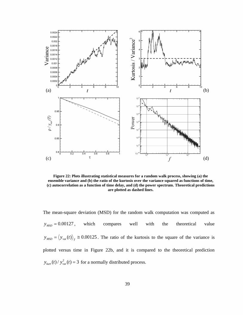
Figure 22: Plots illustrating statistical measures for a random walk process, showing (a) the
ensemble variance and (b) the ratio of the kurtosis over the variance squared as functions of time,
(c) autocorrelation as a function of time delay, and (d) the power spectrum. Theoretical predictions
are plotted as dashed lines.
The mean-square deviation (MSD) for the random walk computation was computed as
00127.0=MSDy , which compares well with the theoretical value
00125.0)(var =TMSD tyy . The ratio of the kurtosis to the square of the variance is
plotted versus time in Figure 22b, and it is compared to the theoretical prediction
3)(/)( 2
var =tytykurt for a normally distributed process.
(a) (b)
(c) (d)
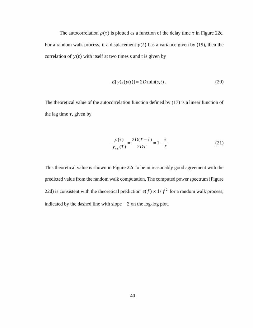
40
The autocorrelation 𝜌(𝜏) is plotted as a function of the delay time 𝜏 in Figure 22c.
For a random walk process, if a displacement 𝑦(𝑡) has a variance given by (19), then the
correlation of 𝑦(𝑡) with itself at two times s and t is given by
),min(2)]()([ tsDtysyE = . (20)
The theoretical value of the autocorrelation function defined by (17) is a linear function of
the lag time 𝜏, given by
TDT
TD
Ty
−=
−= 1
2
)(2
)(
)(
var
. (21)
This theoretical value is shown in Figure 22c to be in reasonably good agreement with the
predicted value from the random walk computation. The computed power spectrum (Figure
22d) is consistent with the theoretical prediction 2/1)( ffe for a random walk process,
indicated by the dashed line with slope −2 on the log-log plot.
41
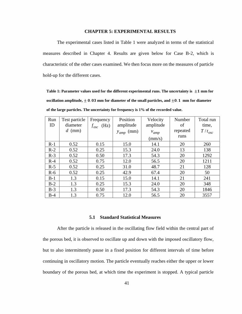
CHAPTER 5: EXPERIMENTAL RESULTS
The experimental cases listed in Table 1 were analyzed in terms of the statistical
measures described in Chapter 4. Results are given below for Case B-2, which is
characteristic of the other cases examined. We then focus more on the measures of particle
hold-up for the different cases.
Table 1: Parameter values used for the different experimental runs. The uncertainty is ±𝟏 mm for
oscillation amplitude, ± 𝟎. 𝟎𝟑 mm for diameter of the small particles, and ±𝟎. 𝟏 mm for diameter
of the large particles. The uncertainty for frequency is 1% of the recorded value.
Run
ID
Test particle
diameter
d (mm)
Frequency
oscf (Hz)
Position
amplitude
ampy (mm)
Velocity
amplitude
ampv
(mm/s)
Number
of
repeated
runs
Total run
time,
osctT /
R-1 0.52 0.15 15.0 14.1 20 260
R-2 0.52 0.25 15.3 24.0 13 138
R-3 0.52 0.50 17.3 54.3 20 1292
R-4 0.52 0.75 12.0 56.5 20 1211
R-5 0.52 0.25 31.0 48.7 21 128
R-6 0.52 0.25 42.9 67.4 20 50
B-1 1.3 0.15 15.0 14.1 21 241
B-2 1.3 0.25 15.3 24.0 20 348
B-3 1.3 0.50 17.3 54.3 20 1846
B-4 1.3 0.75 12.0 56.5 20 3557
5.1 Standard Statistical Measures
After the particle is released in the oscillating flow field within the central part of
the porous bed, it is observed to oscillate up and down with the imposed oscillatory flow,
but to also intermittently pause in a fixed position for different intervals of time before
continuing in oscillatory motion. The particle eventually reaches either the upper or lower
boundary of the porous bed, at which time the experiment is stopped. A typical particle
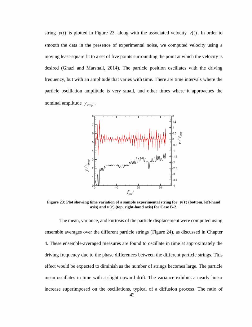
42
string )(ty is plotted in Figure 23, along with the associated velocity )(tv . In order to
smooth the data in the presence of experimental noise, we computed velocity using a
moving least-square fit to a set of five points surrounding the point at which the velocity is
desired (Ghazi and Marshall, 2014). The particle position oscillates with the driving
frequency, but with an amplitude that varies with time. There are time intervals where the
particle oscillation amplitude is very small, and other times where it approaches the
nominal amplitude ampy .
Figure 23: Plot showing time variation of a sample experimental string for 𝒚(𝒕) (bottom, left-hand
axis) and 𝒗(𝒕) (top, right-hand axis) for Case B-2.
The mean, variance, and kurtosis of the particle displacement were computed using
ensemble averages over the different particle strings (Figure 24), as discussed in Chapter
4. These ensemble-averaged measures are found to oscillate in time at approximately the
driving frequency due to the phase differences between the different particle strings. This
effect would be expected to diminish as the number of strings becomes large. The particle
mean oscillates in time with a slight upward drift. The variance exhibits a nearly linear
increase superimposed on the oscillations, typical of a diffusion process. The ratio of
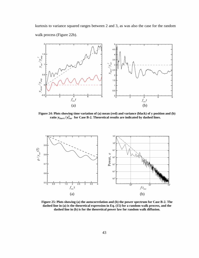
43
kurtosis to variance squared ranges between 2 and 3, as was also the case for the random
walk process (Figure 22b).
Figure 24: Plots showing time variation of (a) mean (red) and variance (black) of y position and (b)
ratio 𝒚𝒌𝒖𝒓𝒕 𝒚𝒗𝒂𝒓𝟐⁄ for Case B-2. Theoretical results are indicated by dashed lines.
Figure 25: Plots showing (a) the autocorrelation and (b) the power spectrum for Case B-2. The
dashed line in (a) is the theoretical expression in Eq. (15) for a random-walk process, and the
dashed line in (b) is for the theoretical power law for random walk diffusion.
(a) (b)
(a) (b)
44
The autocorrelation is plotted in Figure 25a as a function of the dimensionless lag
time oscf . It is noted that for a random walk diffusion process, the autocorrelation is a
linear function of lag time with decreasing slope, indicated by the dashed line in Figure
25a. For a purely oscillating process, the signal is perfectly correlated once every
oscillation period, and the resulting autocorrelation is an oscillatory function. The curve
observed in Figure 25a for an oscillatory diffusion process is a combination of these two
trends, consisting of an oscillating function with a downward trending mean value. The
power spectrum plotted in Figure 25b is found to be similar to that for random walk
processes (Figure 22d), with a variation closely following a line with slope of -2 on the
log-log plot, indicating a 2/1)( ffe power-law dependence with frequency. A
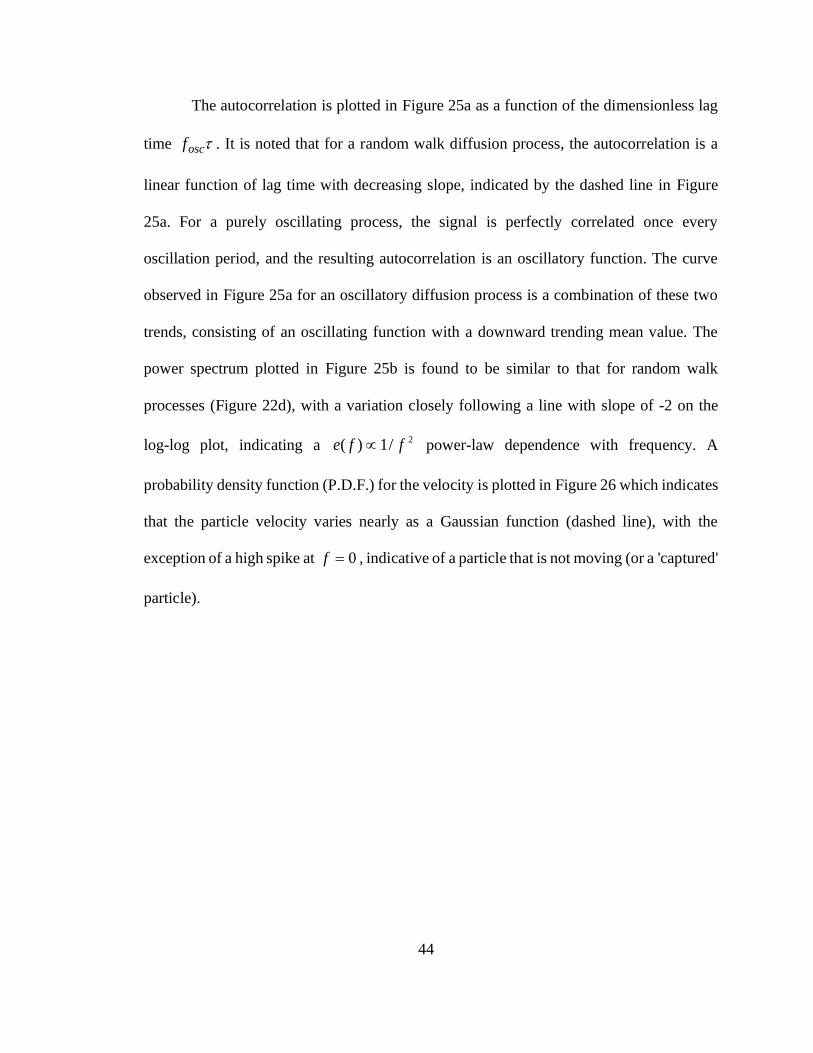
probability density function (P.D.F.) for the velocity is plotted in Figure 26 which indicates
that the particle velocity varies nearly as a Gaussian function (dashed line), with the
exception of a high spike at 0=f , indicative of a particle that is not moving (or a 'captured'
particle).
45
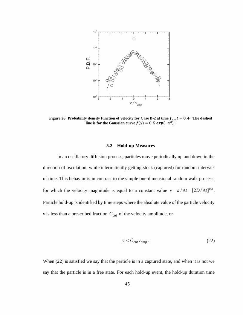
Figure 26: Probability density function of velocity for Case B-2 at time 𝒇𝒐𝒔𝒄𝒕 = 𝟎. 𝟒 . The dashed
line is for the Gaussian curve 𝒇(𝒙) = 𝟎. 𝟓 𝒆𝒙𝒑(−𝒙𝟐) .
5.2 Hold-up Measures
In an oscillatory diffusion process, particles move periodically up and down in the
direction of oscillation, while intermittently getting stuck (captured) for random intervals
of time. This behavior is in contrast to the simple one-dimensional random walk process,
for which the velocity magnitude is equal to a constant value 2/1]/2[/ tDtv == .
Particle hold-up is identified by time steps where the absolute value of the particle velocity
v is less than a prescribed fraction cutC of the velocity amplitude, or
ampcutvCv . (22)
When (22) is satisfied we say that the particle is in a captured state, and when it is not we
say that the particle is in a free state. For each hold-up event, the hold-up duration time
46
𝑡ℎ𝑜𝑙𝑑 is set equal to the number of consecutive cycles during which the particle is in a
captured state times the time step Δ𝑡. The set of hold-up duration times for all strings in an
ensemble was sorted into a set of bins, and the number of hold-up events falling in each
bin is denoted as 𝑁ℎ𝑜𝑙𝑑,𝑖, where the bin number 𝑖 corresponds to a certain interval of the
hold-up duration time 𝑡ℎ𝑜𝑙𝑑. A plot showing the values of the normalized number of hold-
up events 𝑁ℎ𝑜𝑙𝑑 (𝑁𝑡𝑜𝑡𝑓𝑜𝑠𝑐Δ𝑡𝑏𝑖𝑛)⁄ for these bins is given in Figure 27 for the case B-2,
comparing results for 𝐶𝑐𝑢𝑡 values of 0.1, 0.2 and 0.3 for a plot with 50 bins of uniform
width. In this plot, 𝑁𝑡𝑜𝑡 is the total number of hold-up events and Δ𝑡𝑏𝑖𝑛 is the bin width.
For larger 𝐶𝑐𝑢𝑡 values there are more long-duration hold-up events (with larger values
of 𝑡ℎ𝑜𝑙𝑑), whereas for smaller 𝐶𝑐𝑢𝑡 values the long duration hold-up events tend to be
broken up into a series of shorter duration events. However, the symbols in Figure 27 seem
to be scattered about a similar curve for all three cases, suggesting that a common
distribution of hold-up events might apply.
Figure 27: Plot showing the normalized number of hold-up events as a function of the
dimensionless hold time 𝒇𝒐𝒔𝒄𝒕𝒉𝒐𝒍𝒅 for Case B-2 with different values of the cut-off coefficient:
𝑪𝒄𝒖𝒕 = 𝟎. 𝟏 (squares), 𝟎. 𝟐 (deltas), and 𝟎. 𝟑 (circles).
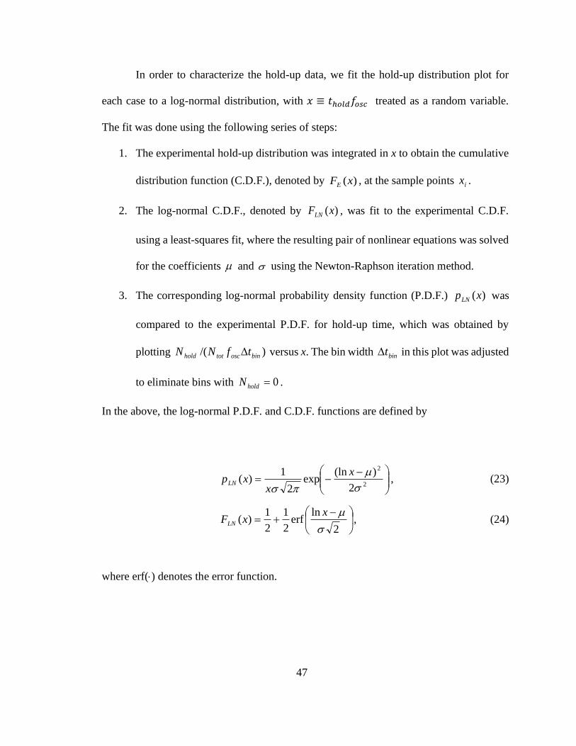
47
In order to characterize the hold-up data, we fit the hold-up distribution plot for
each case to a log-normal distribution, with 𝑥 ≡ 𝑡ℎ𝑜𝑙𝑑𝑓𝑜𝑠𝑐 treated as a random variable.
The fit was done using the following series of steps:
1. The experimental hold-up distribution was integrated in x to obtain the cumulative
distribution function (C.D.F.), denoted by )(xFE , at the sample points ix .
2. The log-normal C.D.F., denoted by )(xFLN , was fit to the experimental C.D.F.
using a least-squares fit, where the resulting pair of nonlinear equations was solved
for the coefficients and using the Newton-Raphson iteration method.
3. The corresponding log-normal probability density function (P.D.F.) )(xpLN was
compared to the experimental P.D.F. for hold-up time, which was obtained by
plotting )/( binosctothold tfNN versus x. The bin width bint in this plot was adjusted
to eliminate bins with 0=holdN .
In the above, the log-normal P.D.F. and C.D.F. functions are defined by
−−=
2
2
2
)(lnexp
2
1)(
x
xxpLN , (23)
−+=
2
lnerf
2
1
2
1)(
xxFLN , (24)
where erf() denotes the error function.
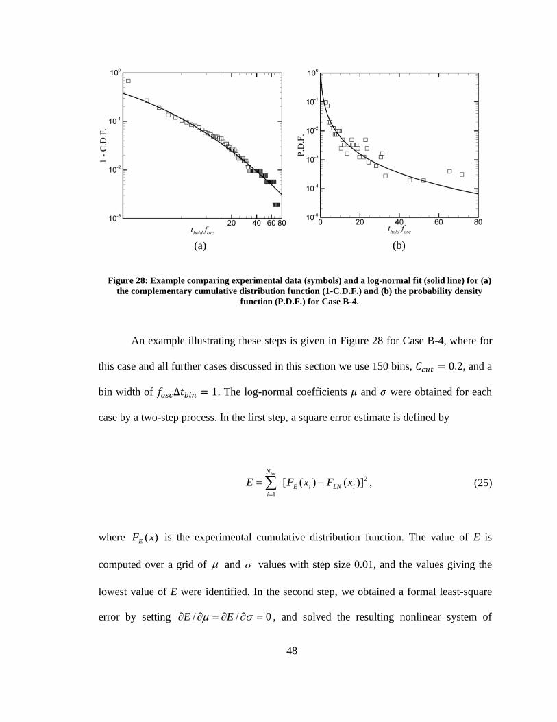
48
Figure 28: Example comparing experimental data (symbols) and a log-normal fit (solid line) for (a)
the complementary cumulative distribution function (1-C.D.F.) and (b) the probability density
function (P.D.F.) for Case B-4.
An example illustrating these steps is given in Figure 28 for Case B-4, where for
this case and all further cases discussed in this section we use 150 bins, 𝐶𝑐𝑢𝑡 = 0.2, and a
bin width of 𝑓𝑜𝑠𝑐Δ𝑡𝑏𝑖𝑛 = 1. The log-normal coefficients 𝜇 and 𝜎 were obtained for each
case by a two-step process. In the first step, a square error estimate is defined by
2
1
)]()([ iLNiE
N
i
xFxFEtot
−==
, (25)
where )(xFE is the experimental cumulative distribution function. The value of E is
computed over a grid of and values with step size 0.01, and the values giving the
lowest value of E were identified. In the second step, we obtained a formal least-square
error by setting 0// == EE , and solved the resulting nonlinear system of
(a) (b)
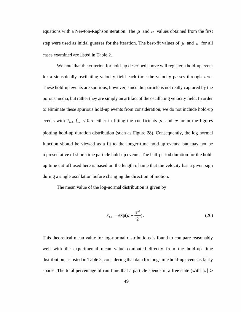
49
equations with a Newton-Raphson iteration. The and values obtained from the first
step were used as initial guesses for the iteration. The best-fit values of and for all
cases examined are listed in Table 2.
We note that the criterion for hold-up described above will register a hold-up event
for a sinusoidally oscillating velocity field each time the velocity passes through zero.
These hold-up events are spurious, however, since the particle is not really captured by the
porous media, but rather they are simply an artifact of the oscillating velocity field. In order
to eliminate these spurious hold-up events from consideration, we do not include hold-up
events with 5.0oschold ft either in fitting the coefficients and or in the figures
plotting hold-up duration distribution (such as Figure 28). Consequently, the log-normal
function should be viewed as a fit to the longer-time hold-up events, but may not be
representative of short-time particle hold-up events. The half-period duration for the hold-
up time cut-off used here is based on the length of time that the velocity has a given sign
during a single oscillation before changing the direction of motion.
The mean value of the log-normal distribution is given by
)2
exp(2
+=LNx . (26)
This theoretical mean value for log-normal distributions is found to compare reasonably
well with the experimental mean value computed directly from the hold-up time
distribution, as listed in Table 2, considering that data for long-time hold-up events is fairly
sparse. The total percentage of run time that a particle spends in a free state (with |𝑣| >
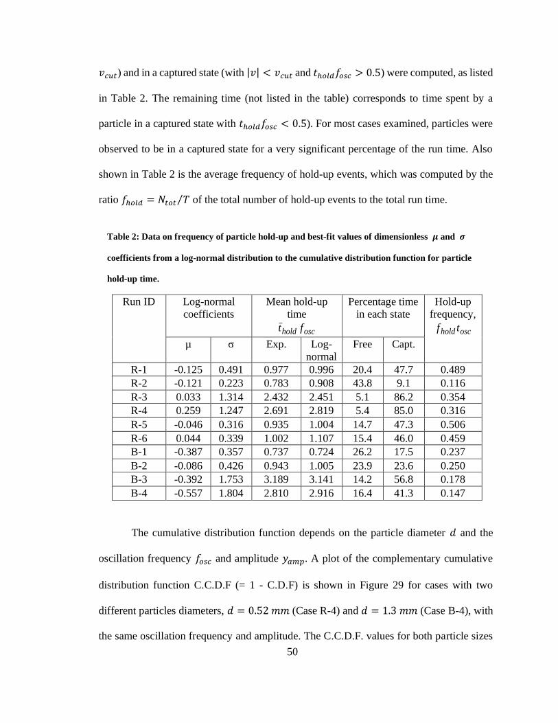
50
𝑣𝑐𝑢𝑡) and in a captured state (with |𝑣| < 𝑣𝑐𝑢𝑡 and 𝑡ℎ𝑜𝑙𝑑𝑓𝑜𝑠𝑐 > 0.5) were computed, as listed
in Table 2. The remaining time (not listed in the table) corresponds to time spent by a
particle in a captured state with 𝑡ℎ𝑜𝑙𝑑𝑓𝑜𝑠𝑐 < 0.5). For most cases examined, particles were
observed to be in a captured state for a very significant percentage of the run time. Also
shown in Table 2 is the average frequency of hold-up events, which was computed by the
ratio 𝑓ℎ𝑜𝑙𝑑 = 𝑁𝑡𝑜𝑡 𝑇⁄ of the total number of hold-up events to the total run time.
Table 2: Data on frequency of particle hold-up and best-fit values of dimensionless 𝝁 and 𝝈
coefficients from a log-normal distribution to the cumulative distribution function for particle
hold-up time.
Run ID Log-normal
coefficients
Mean hold-up
time
oschold ft
Percentage time
in each state
Hold-up
frequency,
oschold tf
µ σ Exp. Log-
normal
Free Capt.
R-1 -0.125 0.491 0.977 0.996 20.4 47.7 0.489
R-2 -0.121 0.223 0.783 0.908 43.8 9.1 0.116
R-3 0.033 1.314 2.432 2.451 5.1 86.2 0.354
R-4 0.259 1.247 2.691 2.819 5.4 85.0 0.316
R-5 -0.046 0.316 0.935 1.004 14.7 47.3 0.506
R-6 0.044 0.339 1.002 1.107 15.4 46.0 0.459
B-1 -0.387 0.357 0.737 0.724 26.2 17.5 0.237
B-2 -0.086 0.426 0.943 1.005 23.9 23.6 0.250
B-3 -0.392 1.753 3.189 3.141 14.2 56.8 0.178
B-4 -0.557 1.804 2.810 2.916 16.4 41.3 0.147
The cumulative distribution function depends on the particle diameter 𝑑 and the
oscillation frequency 𝑓𝑜𝑠𝑐 and amplitude 𝑦𝑎𝑚𝑝. A plot of the complementary cumulative
distribution function C.C.D.F (= 1 - C.D.F) is shown in Figure 29 for cases with two
different particles diameters, 𝑑 = 0.52 𝑚𝑚 (Case R-4) and 𝑑 = 1.3 𝑚𝑚 (Case B-4), with
the same oscillation frequency and amplitude. The C.C.D.F. values for both particle sizes
51
are fairly close, with the difference that the larger particles exhibit more long-duration
hold-up events and the smaller particle experiences more short-duration hold-up events.
Figure 29: Comparison of complementary cumulative distribution function for cases with particle
diameters of 𝒅 = 𝟎. 𝟓𝟐 mm (red squares, Case R-4) and 𝒅 = 𝟏. 𝟑 mm (black deltas, Case B-4).
A comparison of the effect of oscillation frequency on the complementary
cumulative distribution function is shown in Figure 30a for Cases B-1 through B-4 with
frequency varying from 𝑓𝑜𝑠𝑐 = 0.15 − 0.75 𝐻𝑧, all having the same oscillation amplitude
and particle diameter. A comparison of the effect of oscillation amplitude on the
complementary cumulative distribution function is shown in Figure 30b for Cases R-2, R-
5 and R-6, with amplitude varying from 𝑦𝑎𝑚𝑝 = 15.3 − 42.9 𝑚𝑚, all having the same
oscillation frequency and particle diameter. Comparing these C.C.D.F. plots with the
values of run time listed in Table 1, we see that the experimental runs fall into two
categories - cases with relatively short run-time and cases with relatively long run-time.
The C.C.D.F. is similar for all cases with short run-time (Cases R-1, R-2, B-1, B-2, R-5,
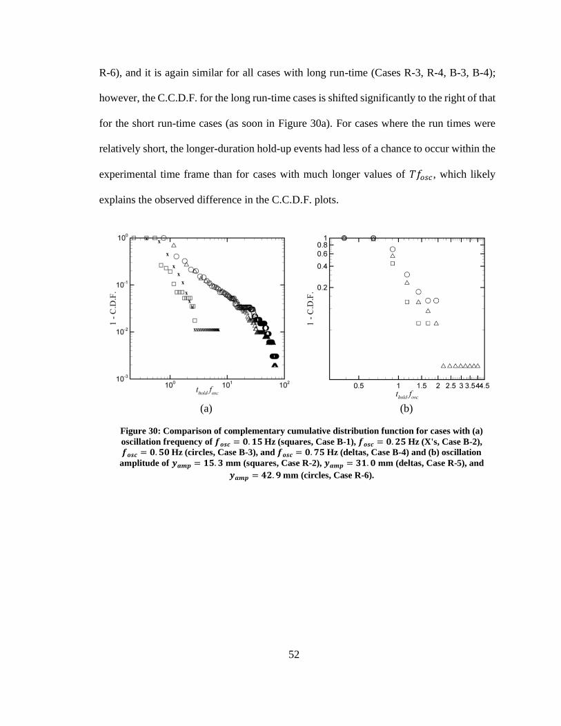
52
R-6), and it is again similar for all cases with long run-time (Cases R-3, R-4, B-3, B-4);
however, the C.C.D.F. for the long run-time cases is shifted significantly to the right of that
for the short run-time cases (as soon in Figure 30a). For cases where the run times were
relatively short, the longer-duration hold-up events had less of a chance to occur within the
experimental time frame than for cases with much longer values of 𝑇𝑓𝑜𝑠𝑐 , which likely
explains the observed difference in the C.C.D.F. plots.
Figure 30: Comparison of complementary cumulative distribution function for cases with (a)
oscillation frequency of 𝒇𝒐𝒔𝒄 = 𝟎. 𝟏𝟓 Hz (squares, Case B-1), 𝒇𝒐𝒔𝒄 = 𝟎. 𝟐𝟓 Hz (X's, Case B-2),
𝒇𝒐𝒔𝒄 = 𝟎. 𝟓𝟎 Hz (circles, Case B-3), and 𝒇𝒐𝒔𝒄 = 𝟎. 𝟕𝟓 Hz (deltas, Case B-4) and (b) oscillation
amplitude of 𝒚𝒂𝒎𝒑 = 𝟏𝟓. 𝟑 mm (squares, Case R-2), 𝒚𝒂𝒎𝒑 = 𝟑𝟏. 𝟎 mm (deltas, Case R-5), and
𝒚𝒂𝒎𝒑 = 𝟒𝟐. 𝟗 mm (circles, Case R-6).
(a) (b)
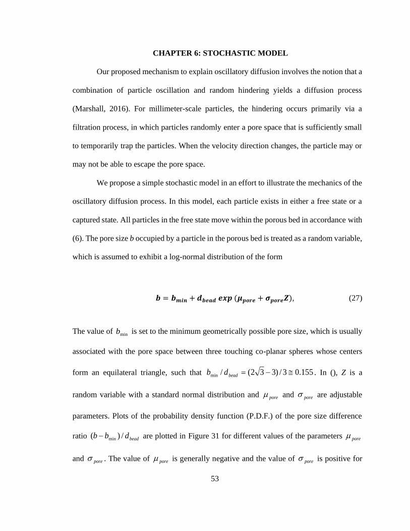
53
CHAPTER 6: STOCHASTIC MODEL
Our proposed mechanism to explain oscillatory diffusion involves the notion that a
combination of particle oscillation and random hindering yields a diffusion process
(Marshall, 2016). For millimeter-scale particles, the hindering occurs primarily via a
filtration process, in which particles randomly enter a pore space that is sufficiently small
to temporarily trap the particles. When the velocity direction changes, the particle may or
may not be able to escape the pore space.
We propose a simple stochastic model in an effort to illustrate the mechanics of the
oscillatory diffusion process. In this model, each particle exists in either a free state or a
captured state. All particles in the free state move within the porous bed in accordance with
(6). The pore size b occupied by a particle in the porous bed is treated as a random variable,
which is assumed to exhibit a log-normal distribution of the form
𝒃 = 𝒃𝒎𝒊𝒏 + 𝒅𝒃𝒆𝒂𝒅 𝒆𝒙𝒑 (𝝁𝒑𝒐𝒓𝒆 + 𝝈𝒑𝒐𝒓𝒆𝒁), (27)
The value of minb is set to the minimum geometrically possible pore size, which is usually
associated with the pore space between three touching co-planar spheres whose centers
form an equilateral triangle, such that 155.03/)332(/min −=beaddb . In (), Z is a
random variable with a standard normal distribution and pore and pore are adjustable
parameters. Plots of the probability density function (P.D.F.) of the pore size difference
ratio beaddbb /)( min− are plotted in Figure 31 for different values of the parameters pore
and pore . The value of pore is generally negative and the value of pore is positive for
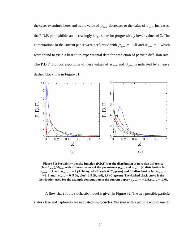
54
the cases examined here, and as the value of pore decreases or the value of pore increases,
the P.D.F. plot exhibits an increasingly large spike for progressively lower values of Z. The
computations in the current paper were performed with 8.1−=pore and pore = 1, which
were found to yield a best fit to experimental data for prediction of particle diffusion rate.
The P.D.F. plot corresponding to these values of pore and pore is indicated by a heavy
dashed black line in Figure 31.
Figure 31: Probability density function (P.D.F.) for the distribution of pore size difference
(𝒃 − 𝒃𝒎𝒊𝒏) 𝒅𝒃𝒆𝒂𝒅⁄ with different values of the parameters 𝝁𝒑𝒐𝒓𝒆 and 𝝈𝒑𝒐𝒓𝒆: (a) distribution for
𝝈𝒑𝒐𝒓𝒆 = 𝟏 and 𝝁𝒑𝒐𝒓𝒆 = −𝟑 (A, blue), −𝟐 (B, red), 0 (C, green) and (b) distribution for 𝝁𝒑𝒐𝒓𝒆 =
−𝟏. 𝟖 and 𝝈𝒑𝒐𝒓𝒆 = 𝟎. 𝟓 (A, blue), 1.5 (B, red), 2.0 (C, green). The dashed black curve is the
distribution used for the example computation in the current paper (𝝁𝒑𝒐𝒓𝒆 = −𝟏. 𝟖,𝝈𝒑𝒐𝒓𝒆 = 𝟏. 𝟎).
A flow chart of the stochastic model is given in Figure 32. The two possible particle
states - free and captured - are indicated using circles. We start with a particle with diameter
(a) (b)
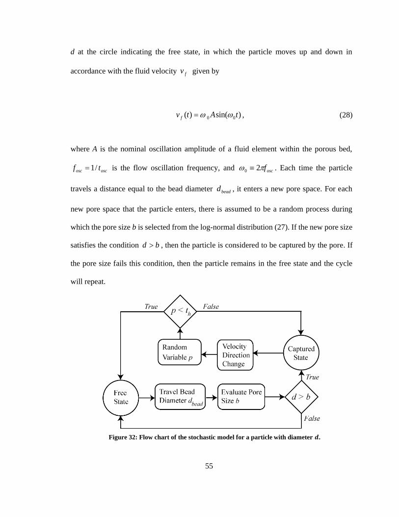
55
d at the circle indicating the free state, in which the particle moves up and down in
accordance with the fluid velocity fv given by
)sin()( 00 tAtv f = , (28)
where A is the nominal oscillation amplitude of a fluid element within the porous bed,
oscosc tf /1= is the flow oscillation frequency, and oscf 20 . Each time the particle
travels a distance equal to the bead diameter beadd , it enters a new pore space. For each
new pore space that the particle enters, there is assumed to be a random process during
which the pore size b is selected from the log-normal distribution (27). If the new pore size
satisfies the condition bd , then the particle is considered to be captured by the pore. If
the pore size fails this condition, then the particle remains in the free state and the cycle
will repeat.
Figure 32: Flow chart of the stochastic model for a particle with diameter 𝒅.
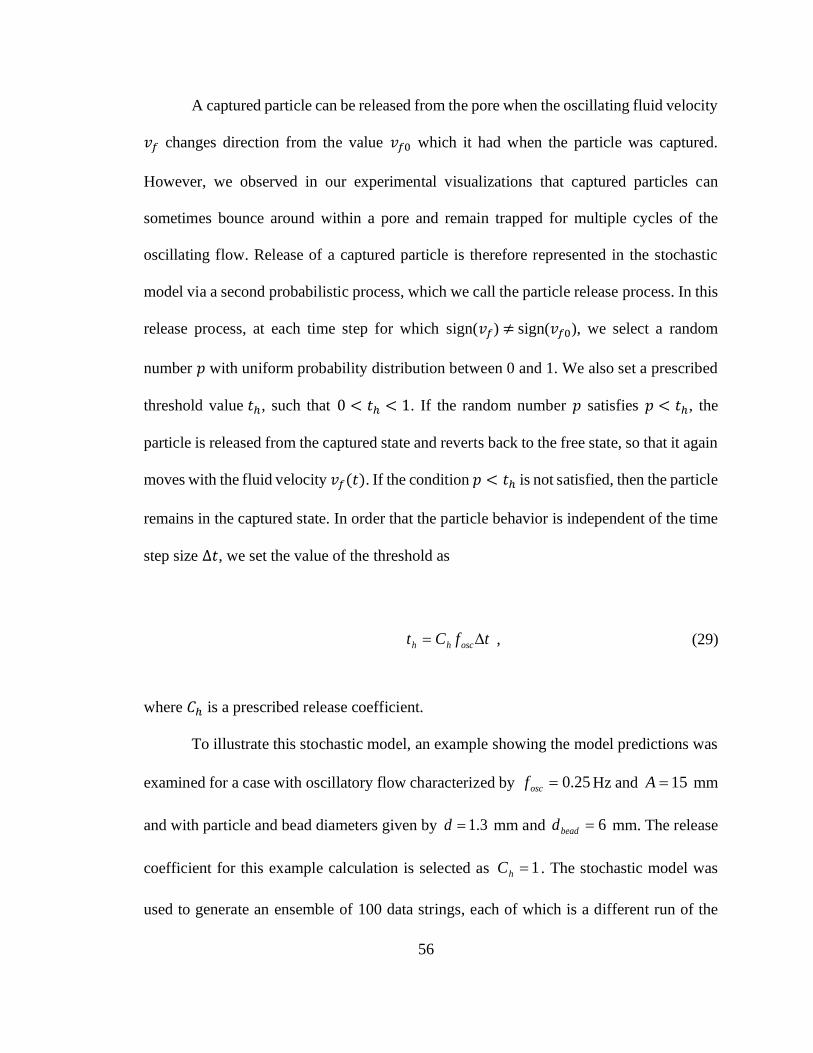
56
A captured particle can be released from the pore when the oscillating fluid velocity
𝑣𝑓 changes direction from the value 𝑣𝑓0 which it had when the particle was captured.
However, we observed in our experimental visualizations that captured particles can
sometimes bounce around within a pore and remain trapped for multiple cycles of the
oscillating flow. Release of a captured particle is therefore represented in the stochastic
model via a second probabilistic process, which we call the particle release process. In this
release process, at each time step for which sign(𝑣𝑓) ≠ sign(𝑣𝑓0), we select a random
number 𝑝 with uniform probability distribution between 0 and 1. We also set a prescribed
threshold value 𝑡ℎ, such that 0 < 𝑡ℎ < 1. If the random number 𝑝 satisfies 𝑝 < 𝑡ℎ, the
particle is released from the captured state and reverts back to the free state, so that it again
moves with the fluid velocity 𝑣𝑓(𝑡). If the condition 𝑝 < 𝑡ℎ is not satisfied, then the particle
remains in the captured state. In order that the particle behavior is independent of the time
step size Δ𝑡, we set the value of the threshold as
tfCt oschh = , (29)
where 𝐶ℎ is a prescribed release coefficient.
To illustrate this stochastic model, an example showing the model predictions was
examined for a case with oscillatory flow characterized by 25.0=oscf Hz and 15=A mm
and with particle and bead diameters given by 3.1=d mm and 6=beadd mm. The release
coefficient for this example calculation is selected as 1=hC . The stochastic model was
used to generate an ensemble of 100 data strings, each of which is a different run of the
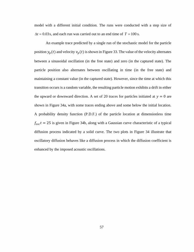
57
model with a different initial condition. The runs were conducted with a step size of
03.0=t s, and each run was carried out to an end time of 100=T s.
An example trace predicted by a single run of the stochastic model for the particle
position 𝑦𝑝(𝑡) and velocity 𝑣𝑝(𝑡) is shown in Figure 33. The value of the velocity alternates
between a sinusoidal oscillation (in the free state) and zero (in the captured state). The
particle position also alternates between oscillating in time (in the free state) and
maintaining a constant value (in the captured state). However, since the time at which this
transition occurs is a random variable, the resulting particle motion exhibits a drift in either
the upward or downward direction. A set of 20 traces for particles initiated at 𝑦 = 0 are
shown in Figure 34a, with some traces ending above and some below the initial location.
A probability density function (P.D.F.) of the particle location at dimensionless time
𝑓𝑜𝑠𝑐𝑡 = 25 is given in Figure 34b, along with a Gaussian curve characteristic of a typical
diffusion process indicated by a solid curve. The two plots in Figure 34 illustrate that
oscillatory diffusion behaves like a diffusion process in which the diffusion coefficient is
enhanced by the imposed acoustic oscillations.
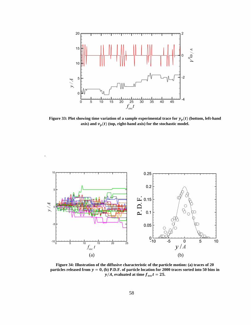
58
Figure 33: Plot showing time variation of a sample experimental trace for 𝒚𝒑(𝒕) (bottom, left-hand
axis) and 𝒗𝒑(𝒕) (top, right-hand axis) for the stochastic model.
.
Figure 34: Illustration of the diffusive characteristic of the particle motion: (a) traces of 20
particles released from 𝒚 = 𝟎, (b) P.D.F. of particle location for 2000 traces sorted into 50 bins in
𝒚 𝑨⁄ , evaluated at time 𝒇𝒐𝒔𝒄𝒕 = 𝟐𝟓.
(a) (b)
59
Ensemble-averaged data for the set of 20 data strings are shown in Figure 35a and
35b in comparison to the experimental data for Case B-2. In Figure 35a, the variance is
observed to increase in time by fluctuating about a nearly linear increase. A dashed line
with the same slope as the linear increase passing through the origin is plotted in Figure
35a. Figure 35b shows the ratio of the kurtosis to the square of the variance for )(ty , which
after an initial transient oscillates about the theoretical value of 3 for a normally-distributed
process (dashed line). The computed autocorrelation for the stochastic model predictions
are plotted against the lag time in Figure 35c. The predicted autocorrelation curve is nearly
straight, as is also the case for a random walk process. The autocorrelation function for the
experimental data in Case B-2 exhibited more oscillation than the stochastic model
predictions, but both curves are reasonably close to each other. The power spectrum for the
stochastic model predictions is plotted in Figure 35d, with a dashed line representing the
2− fe power law on the log-log plot. This power law gives a fairly close fit to the mean
slope of the data, as was also the case for the random walk process and the experimental
data.
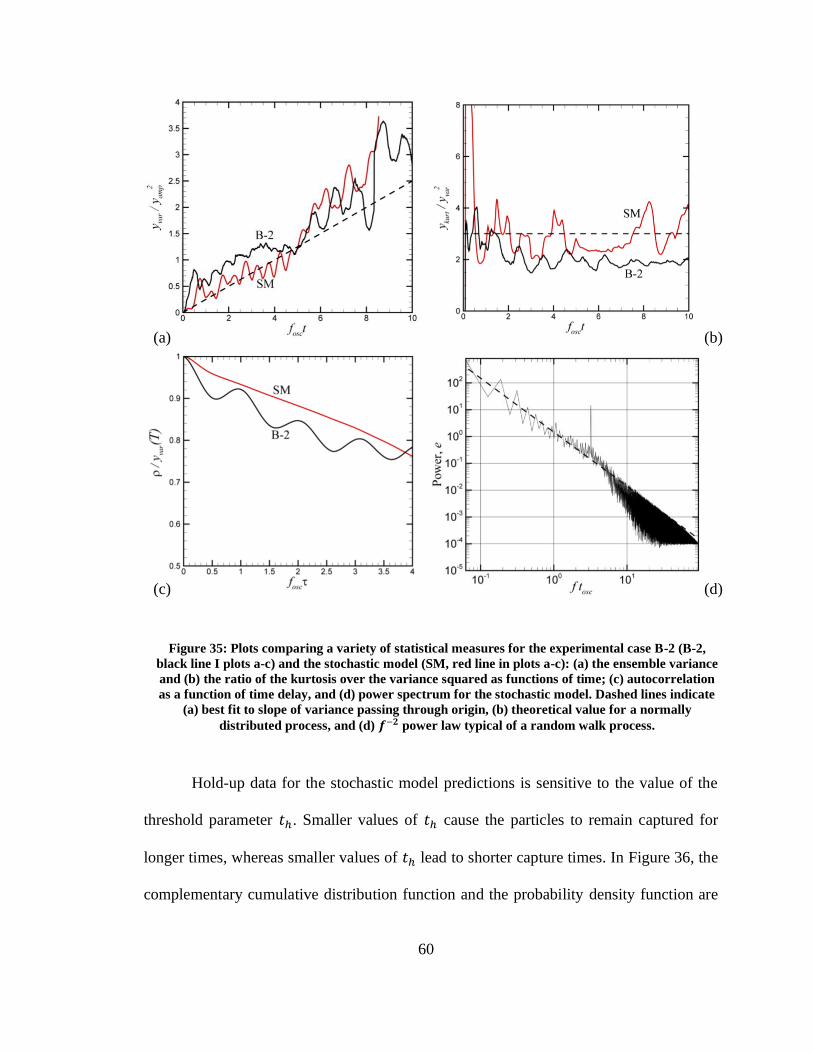
60
Figure 35: Plots comparing a variety of statistical measures for the experimental case B-2 (B-2,
black line I plots a-c) and the stochastic model (SM, red line in plots a-c): (a) the ensemble variance
and (b) the ratio of the kurtosis over the variance squared as functions of time; (c) autocorrelation
as a function of time delay, and (d) power spectrum for the stochastic model. Dashed lines indicate
(a) best fit to slope of variance passing through origin, (b) theoretical value for a normally
distributed process, and (d) 𝒇−𝟐 power law typical of a random walk process.
Hold-up data for the stochastic model predictions is sensitive to the value of the
threshold parameter 𝑡ℎ. Smaller values of 𝑡ℎ cause the particles to remain captured for
longer times, whereas smaller values of 𝑡ℎ lead to shorter capture times. In Figure 36, the
complementary cumulative distribution function and the probability density function are
(b)
(c) (d)
(a)
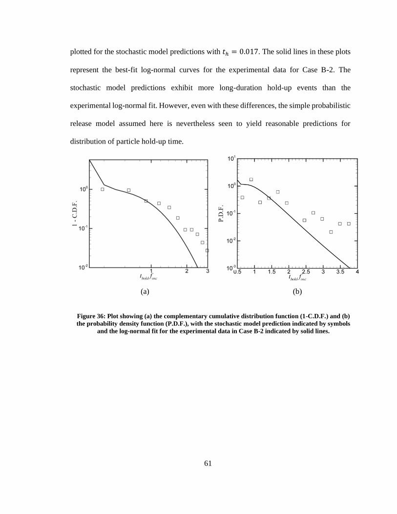
61
plotted for the stochastic model predictions with 𝑡ℎ = 0.017. The solid lines in these plots
represent the best-fit log-normal curves for the experimental data for Case B-2. The
stochastic model predictions exhibit more long-duration hold-up events than the
experimental log-normal fit. However, even with these differences, the simple probabilistic
release model assumed here is nevertheless seen to yield reasonable predictions for
distribution of particle hold-up time.
Figure 36: Plot showing (a) the complementary cumulative distribution function (1-C.D.F.) and (b)
the probability density function (P.D.F.), with the stochastic model prediction indicated by symbols
and the log-normal fit for the experimental data in Case B-2 indicated by solid lines.
(a) (b)
62
CHAPTER 7: PARAMETRIC STUDY OF STOCHASTIC MODEL AND
COMPARISON TO CTRW THEORY
Continuous time random walk (CTRW) is a generalization of the random walk
process in which particles wait for a random time increment before jumping between states
(Montroll and Weiss, 1965; Balakrishnan and Venkataraman, 1981a). This basic model
was generalized by Balakrishnan and Venkataraman (1981b; hereinafter referred to as
BV81b) to the problem of oscillatory diffusion, where it was assumed that particles
fluctuate back and forth between an oscillatory state and a random jump state with constant
velocity 0v , and that the transition time between these two states is a random variable.
Assuming that the transitions between these states occurs via a series of uncorrelated binary
decisions (i.e., a set of Bernoulli trials), BV81b concluded that the holding time distribution
for each state would be of the form of a Poisson distribution, which we denote by )(tp for
the oscillatory state and by )(tq for the random jump state. In the limit of many state
transitions, we assume that these distributions approach the exponential form
)/exp()( 0osctftp −= , )/exp()( 1osctftq −= , (30)
where 0 and 1 are the dimensionless average holding times in the oscillatory and jump
states, respectively. The oscillatory diffusion examined in the current paper can be regarded
as a special case of that examined in BV81b in which we let the jump velocity 00 =v , so
that the particle is stationary (or captured) in the jump state. We henceforth refer to the
jump state of BV81b as the captured state in the current model.
63
The hold-up time distribution for particle capture in the stochastic model
predictions is sensitive to the value of the release coefficient 𝐶ℎ in (29) which is used to
determine whether to release a particle or retain it in a captured state. Small values of 𝐶ℎ
cause particles to remain captured for longer times than do larger values of 𝐶ℎ. The
complementary cumulative distribution function (C.C.D.F.) and the probability density
function (P.D.F.) for the hold-up time variable in the captured state are plotted for the
example problem with 𝐶ℎ = 1 in Figure 37. In this plot, particle capture is identified as
occurring for any time step where the absolute value of the particle velocity 𝑣𝑝(𝑡) is less
than a fraction 𝐶𝑐𝑢𝑡 of the velocity amplitude 𝑣𝑎𝑚𝑝 = 𝜔0𝐴 (22), where 𝐴 = 𝑦𝑎𝑚𝑝.
For the example case shown in Figure 37, we selected 𝐶𝑐𝑢𝑡 = 0.1. The C.C.D.F.
data in Figure 37a was fit using the exponential probability distribution (30), which for a
semi-logarithmic plot yields a linear expression that passes through the point (0,1) and has
slope −1 𝜏1⁄ . The value of the mean holding-time 𝜏1 for the captured state was determined
using a least-square linear regression to the logarithm of the C.C.D.F., which was selected
to give the tails of the distribution equal weight in the fit to the values near the initial time.
This procedure yielded an estimate 𝜏1 = 1.82 with a coefficient of determination of 𝑟2 =
0.98, which is indicated by the solid black line in Figure 37. The uncertainty in the estimate
of 1 is evaluated using a 95% confidence interval, yielding upper and lower bounds for
the fit line indicated by the dashed lines in Figure 37.
The C.C.D.F. and P.D.F for the free oscillation time distribution are plotted in
Figure 38. The best-fit exponential distribution is indicated in these plots by a solid line,
and the 95% confidence interval is indicated by dashed lines. The average holding-time
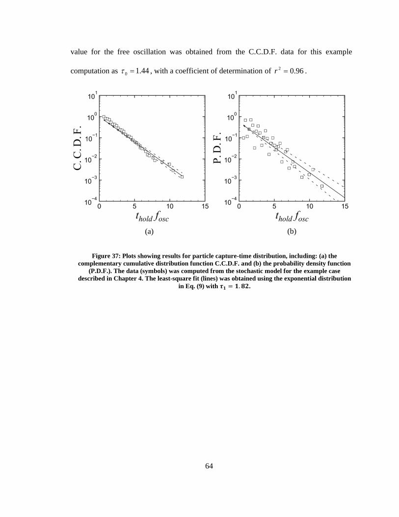
64
value for the free oscillation was obtained from the C.C.D.F. data for this example
computation as 44.10 = , with a coefficient of determination of 96.02 =r .
Figure 37: Plots showing results for particle capture-time distribution, including: (a) the
complementary cumulative distribution function C.C.D.F. and (b) the probability density function
(P.D.F.). The data (symbols) was computed from the stochastic model for the example case
described in Chapter 4. The least-square fit (lines) was obtained using the exponential distribution
in Eq. (9) with 𝝉𝟏 = 𝟏. 𝟖𝟐.
(a) (b)
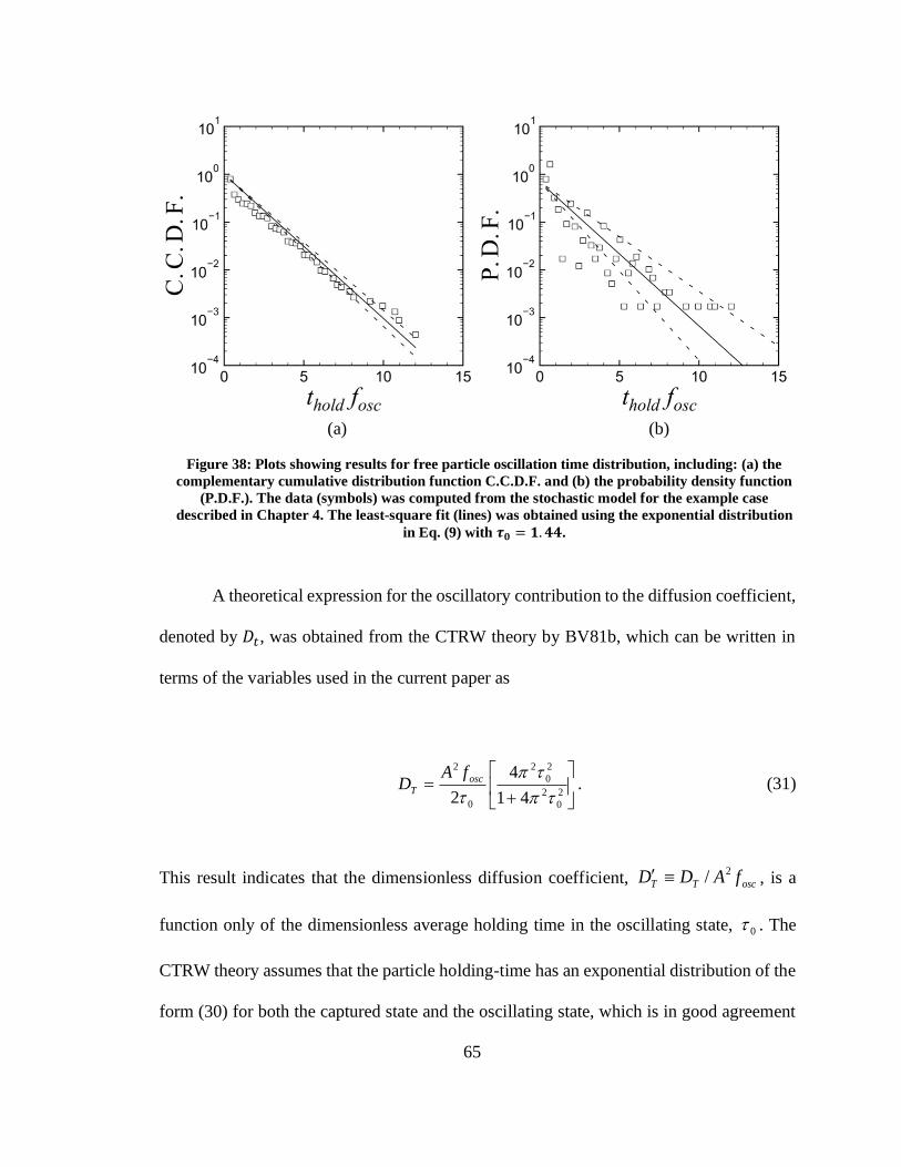
65
Figure 38: Plots showing results for free particle oscillation time distribution, including: (a) the
complementary cumulative distribution function C.C.D.F. and (b) the probability density function
(P.D.F.). The data (symbols) was computed from the stochastic model for the example case
described in Chapter 4. The least-square fit (lines) was obtained using the exponential distribution
in Eq. (9) with 𝝉𝟎 = 𝟏. 𝟒𝟒.
A theoretical expression for the oscillatory contribution to the diffusion coefficient,
denoted by 𝐷𝑡, was obtained from the CTRW theory by BV81b, which can be written in
terms of the variables used in the current paper as
+=
2
0
2
2
0
2
0
2
41
4
2
osc
T
fAD . (31)
This result indicates that the dimensionless diffusion coefficient, oscTT fADD 2/ , is a
function only of the dimensionless average holding time in the oscillating state, 0 . The
CTRW theory assumes that the particle holding-time has an exponential distribution of the
form (30) for both the captured state and the oscillating state, which is in good agreement
(a) (b)
66
with the predictions of our stochastic model (as shown in Figure 37 and Figure 38).
However, there are also several differences between our stochastic model assumptions and
the CTRW theory. One difference is that the stochastic model only allows the particle to
become captured after it has traveled a distance equal to the bead diameter, whereas the
CTRW theory has no minimum travel distance for transition of the particle state. Secondly,
the stochastic model only allows particle release from a captured state during times where
the velocity is opposite in sign to that at which the capture occurred. No such restriction is
found in the CTRW theory.
A parametric study was conducted to test sensitivity of the stochastic model to
various physical and numerical parameters, and to compare predicted diffusion coefficient
values with those of the CTRW theory. The numerical parameters examined include the
dimensionless time step tft osc= , the velocity cut-off coefficient cutC used in (22) for
assigning a particle to a captured state, and the particle release coefficient hC in (29). The
physical parameters examined include the ratio of oscillation amplitude to bead diameter
beaddA / , the ratio of particle diameter to bead diameter beaddd / , and the pore size
parameter pore . The dimensionless diffusion coefficient SD from the stochastic model
was computed for each case using the variance data from the model as
td
ydDS
= var
2
1. (32)
67
where 2
var / Ayyvan = and tft osc= are the dimensionless variance and time, respectively.
The derivative in (32) was obtained using a linear fit to the variance data obtained by linear
regression. The comparison theoretical value of the dimensionless diffusion coefficient
from CTRW theory, TD , was calculated using (31) with the average holding time 0 for
the free oscillation state extracted from the stochastic model data using a least-square fit of
the exponential C.C.D.F. distribution, as shown in Figure 38.
It is noted that the stochastic model is dependent on the values of a series of random
numbers, and as a consequence the predicted values of the dimensionless diffusion
coefficient obtained from the stochastic model, SD , are not the same for two repeated runs
of the code, even if all parameter values are the same. We also observe variation between
runs for the value of 0 , which therefore results in fluctuations in the theoretical prediction
for TD from (31). In order to quantify the size of the fluctuations in diffusion coefficient
values, we performed two sets of experiments by repeated runs for a 'standard case', for
which the dimensionless parameter values are given as follows:
1.0=cutC , 1=hC , 0083.0=t , 55.2/ =beaddA ,
217.0/ =beaddd , 155.0/min =beaddb , 1=pore , 8.1−=pore . (33)
which is consistent with the example case described in Chapter 4. The stochastic model
computation was repeated for these parameter values both 20 times and 100 times. The
mean and standard deviation of the predicted values of SD and TD for each of these sets
of runs are recorded in Table 3. The standard deviation of the stochastic model prediction
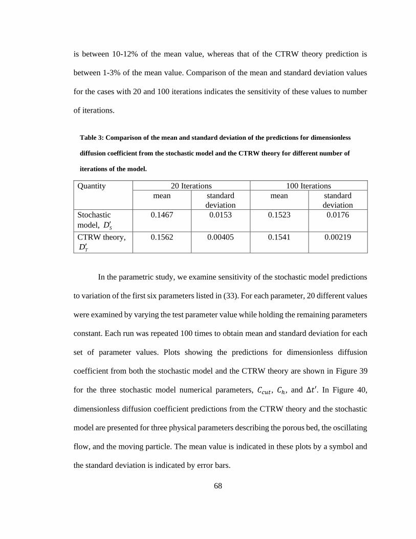
68
is between 10-12% of the mean value, whereas that of the CTRW theory prediction is
between 1-3% of the mean value. Comparison of the mean and standard deviation values
for the cases with 20 and 100 iterations indicates the sensitivity of these values to number
of iterations.
Table 3: Comparison of the mean and standard deviation of the predictions for dimensionless
diffusion coefficient from the stochastic model and the CTRW theory for different number of
iterations of the model.
Quantity 20 Iterations 100 Iterations
mean standard
deviation
mean standard
deviation
Stochastic
model, SD
0.1467 0.0153 0.1523 0.0176
CTRW theory,
TD
0.1562 0.00405 0.1541 0.00219
In the parametric study, we examine sensitivity of the stochastic model predictions
to variation of the first six parameters listed in (33). For each parameter, 20 different values
were examined by varying the test parameter value while holding the remaining parameters
constant. Each run was repeated 100 times to obtain mean and standard deviation for each
set of parameter values. Plots showing the predictions for dimensionless diffusion
coefficient from both the stochastic model and the CTRW theory are shown in Figure 39
for the three stochastic model numerical parameters, 𝐶𝑐𝑢𝑡, 𝐶ℎ, and Δ𝑡′. In Figure 40,
dimensionless diffusion coefficient predictions from the CTRW theory and the stochastic
model are presented for three physical parameters describing the porous bed, the oscillating
flow, and the moving particle. The mean value is indicated in these plots by a symbol and
the standard deviation is indicated by error bars.
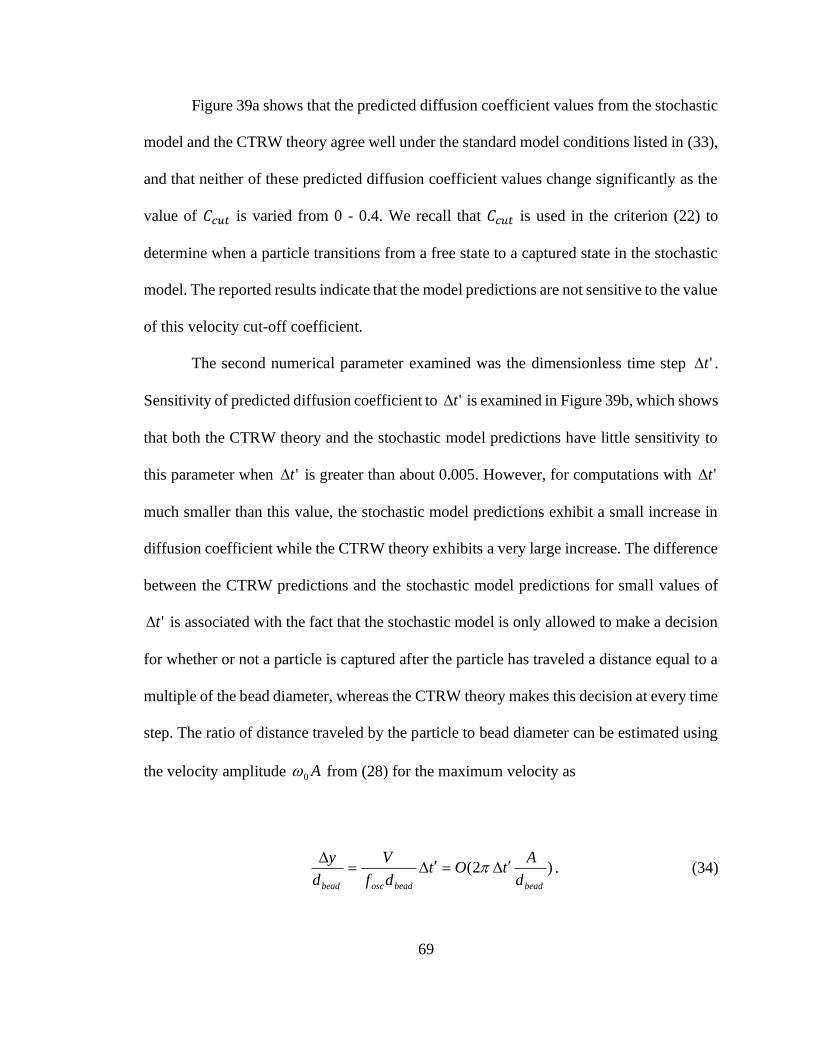
69
Figure 39a shows that the predicted diffusion coefficient values from the stochastic
model and the CTRW theory agree well under the standard model conditions listed in (33),
and that neither of these predicted diffusion coefficient values change significantly as the
value of 𝐶𝑐𝑢𝑡 is varied from 0 - 0.4. We recall that 𝐶𝑐𝑢𝑡 is used in the criterion (22) to
determine when a particle transitions from a free state to a captured state in the stochastic
model. The reported results indicate that the model predictions are not sensitive to the value
of this velocity cut-off coefficient.
The second numerical parameter examined was the dimensionless time step 't .
Sensitivity of predicted diffusion coefficient to 't is examined in Figure 39b, which shows
that both the CTRW theory and the stochastic model predictions have little sensitivity to
this parameter when 't is greater than about 0.005. However, for computations with 't
much smaller than this value, the stochastic model predictions exhibit a small increase in
diffusion coefficient while the CTRW theory exhibits a very large increase. The difference
between the CTRW predictions and the stochastic model predictions for small values of
't is associated with the fact that the stochastic model is only allowed to make a decision
for whether or not a particle is captured after the particle has traveled a distance equal to a
multiple of the bead diameter, whereas the CTRW theory makes this decision at every time
step. The ratio of distance traveled by the particle to bead diameter can be estimated using
the velocity amplitude A0 from (28) for the maximum velocity as
)2(beadbeadoscbead d
AtOt
df
V
d
y==
. (34)
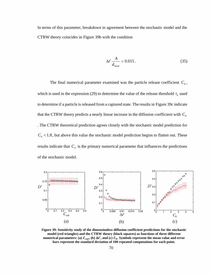
70
In terms of this parameter, breakdown in agreement between the stochastic model and the
CTRW theory coincides in Figure 39b with the condition
015.0beadd
At . (35)
The final numerical parameter examined was the particle release coefficient hC ,
which is used in the expression (29) to determine the value of the release threshold ht used
to determine if a particle is released from a captured state. The results in Figure 39c indicate
that the CTRW theory predicts a nearly linear increase in the diffusion coefficient with hC
. The CTRW theoretical prediction agrees closely with the stochastic model prediction for
8.1hC , but above this value the stochastic model prediction begins to flatten out. These
results indicate that hC is the primary numerical parameter that influences the predictions
of the stochastic model.
Figure 39: Sensitivity study of the dimensionless diffusion coefficient predictions for the stochastic
model (red triangles) and the CTRW theory (black squares) as functions of three different
numerical parameters: (a) 𝑪𝒄𝒖𝒕, (b) 𝚫𝒕′, and (c) 𝑪𝒉. Symbols represent the mean value and error
bars represent the standard deviation of 100 repeated computations for each point.
(a) (b) (c)
71
It would be expected that physical parameters, such as the particle and bead
diameters, the frequency and amplitude of oscillation, and the pore size distribution of the
underlying porous medium, would influence the resulting particle diffusion. From these
variables, we selected three dimensionless physical parameters to examine sensitivity of
the predicted dimensionless diffusion coefficient. The first parameter, 𝐴 𝑑𝑏𝑒𝑎𝑑⁄ , represents
the ratio of the maximum amplitude of particle displacement to the bead diameter. Based
on the criterion (35) with the dimensionless time step given in (33), we would expect the
stochastic model predictions to begin deviating from the CTRW theory for 𝐴 𝑑𝑏𝑒𝑎𝑑 < 1.8⁄ ,
which agrees well with the results in Figure 40a. Because the particle can only change from
a freely oscillating state to a captured state in the stochastic model if it travels a distance
greater than 𝑑𝑏𝑒𝑎𝑑 , the diffusion coefficient predicted by the stochastic model, shown in
Figure 40a, reduces to zero when the maximum distance of particle displacement (2𝐴) is
less than 𝑑𝑏𝑒𝑎𝑑 (or 𝐴 𝑑𝑏𝑒𝑎𝑑 < 1 2⁄⁄ ).
The stochastic model predictions are highly sensitive to the value of the ratio
𝑑 𝑑𝑏𝑒𝑎𝑑⁄ of the particle diameter to the bead diameter. If 𝑑 𝑑𝑏𝑒𝑎𝑑 < 𝑏𝑚𝑖𝑛 𝑑𝑏𝑒𝑎𝑑 = 0.155⁄⁄ ,
the particles will always be smaller than the pore size and pass through the pore without
hold-up, with the consequence that the diffusion coefficient will vanish. We note that the
current stochastic model is based on the assumption that particle capture occurs only from
filtration, and it does not include effects of particle adhesion or other forms of hindering.
On the other hand, as 𝑑 𝑑𝑏𝑒𝑎𝑑⁄ gets large, the likelihood of the particle encountering a pore
that is smaller than the particle becomes progressively smaller. This results in a condition
where the particle becomes continually captured by the surrounding beads, with rapid
decrease in diffusion coefficient. As a result of these two considerations, we see in Figure
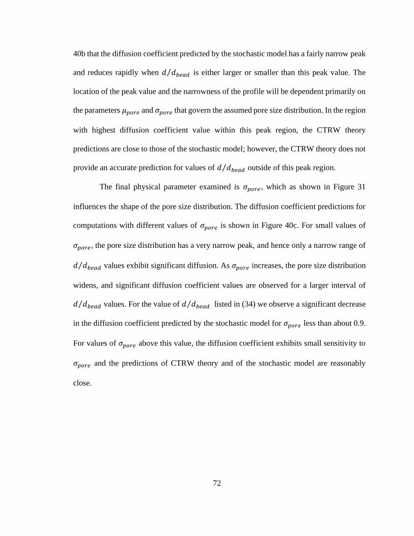
72
40b that the diffusion coefficient predicted by the stochastic model has a fairly narrow peak
and reduces rapidly when 𝑑 𝑑𝑏𝑒𝑎𝑑⁄ is either larger or smaller than this peak value. The
location of the peak value and the narrowness of the profile will be dependent primarily on
the parameters 𝜇𝑝𝑜𝑟𝑒 and 𝜎𝑝𝑜𝑟𝑒 that govern the assumed pore size distribution. In the region
with highest diffusion coefficient value within this peak region, the CTRW theory
predictions are close to those of the stochastic model; however, the CTRW theory does not
provide an accurate prediction for values of 𝑑 𝑑𝑏𝑒𝑎𝑑⁄ outside of this peak region.
The final physical parameter examined is 𝜎𝑝𝑜𝑟𝑒, which as shown in Figure 31
influences the shape of the pore size distribution. The diffusion coefficient predictions for
computations with different values of 𝜎𝑝𝑜𝑟𝑒 is shown in Figure 40c. For small values of
𝜎𝑝𝑜𝑟𝑒, the pore size distribution has a very narrow peak, and hence only a narrow range of
𝑑 𝑑𝑏𝑒𝑎𝑑⁄ values exhibit significant diffusion. As 𝜎𝑝𝑜𝑟𝑒 increases, the pore size distribution
widens, and significant diffusion coefficient values are observed for a larger interval of
𝑑 𝑑𝑏𝑒𝑎𝑑⁄ values. For the value of 𝑑 𝑑𝑏𝑒𝑎𝑑⁄ listed in (34) we observe a significant decrease
in the diffusion coefficient predicted by the stochastic model for 𝜎𝑝𝑜𝑟𝑒 less than about 0.9.
For values of 𝜎𝑝𝑜𝑟𝑒 above this value, the diffusion coefficient exhibits small sensitivity to
𝜎𝑝𝑜𝑟𝑒 and the predictions of CTRW theory and of the stochastic model are reasonably
close.
73
Figure 40: Parametric study of the dimensionless diffusion coefficient predictions for the stochastic
model (red triangles) and the CTRW theory (black squares) as functions of three physical parameters:
(a) 𝑨 𝒅𝒃𝒆𝒂𝒅⁄ , (b) 𝒅 𝒅𝒃𝒆𝒂𝒅⁄ , and (c) 𝝈𝒑𝒐𝒓𝒆. Symbols represent the mean value and error bars represent
the standard deviation of 100 repeated computations for each point.
(a) (b) (c)
74
CHAPTER 8: CONCLUSIONS
A study has been performed on the effect of oscillatory forcing on the enhancement
of diffusion of colloidal particles suspended in a rigid porous bed composed of fixed
spheres. The combination of particle oscillation induced by the oscillatory flow and random
hindering due to interaction with the porous bed produces a type of particle random walk.
This combination leads to particle diffusion in the bed via a process known as oscillatory
diffusion. This process was studied experimentally by following individual particles
moving under an imposed oscillatory flow field in a porous bed of spherical glass beads.
Refractive index matching was used to visualize the particle in the porous bed. The particle
was observed to oscillate up and down with the imposed oscillatory flow field, but also to
intermittently be captured by the porous bed for intervals of various durations. The particle
location data was extracted from video images, from which the particle position and
velocity were determined as functions of time. Experiments were conducted with two
different particle sizes and with various frequencies and amplitudes of the oscillating flow
field. Each condition was repeated approximately 20 times to generate an ensemble of data.
A variety of statistical measures were applied to the experimental data for particle
position within the porous bed in the presence of oscillatory flow, including ensemble
averaging, autocorrelation, spectral analysis, and distribution of particle hold-up times.
These measures were found to exhibit many attributes similar to diffusive processes,
including nearly linear increase in variance with time, nearly linear decrease in
autocorrelation as a function of lag time, and a power-law dependence 2− fe between
spectral power and frequency. At the same time, the experimental data also exhibited some
attributes of an oscillatory process, which resulted in superposition of oscillations for the
75
variance and autocorrelation functions onto the linear dependence typical of diffusive
processes. The distribution of particle hold-up duration that characterizes the intermittent
particle capturing was found to be well fit by a log-normal distribution. The cumulative
distribution plots were used to compare the hold-up distribution data for the different cases
examined.
A stochastic model was developed to describe the oscillatory diffusion process for
particles in a porous bed which involves a transition between a freely oscillating state and
a captured state of the particle. A particle that is initially freely oscillating can become
captured if it moves into a pore space that is smaller than the particle diameter, where the
pore size is assumed to be a log-normally distributed random variable. However, the
particle only moves into a new pore space once it has moved a distance equal to the nominal
diameter of the beads making up the porous bed, which places a limit of the frequency that
particle state transition can occur. Once a particle is captured, it can transition back to the
freely oscillating state during the particle release process, which occurs only when the sign
of the velocity is opposite that at which the initial capture occurred. Particle release is
allowed to occur when the value of a uniformly-distributed random variable is less than a
threshold value. Example computations using this stochastic model exhibit many of the
theoretical characteristics of random walk processes such as a linearly increasing variance,
a ratio of kurtosis to square of variance close to 3.0, and a power spectrum that is inversely
proportional to the square of the frequency. The hold-up time for both the capture and
freely-oscillating states are found to be well fit by exponential probability distributions in
the stochastic model.
76
The oscillatory diffusion process was described in terms of a continuous time
random walk (CTRW) process by Balakrishnan and Venkataraman (1981b) and includes
an analytical solution for the particle diffusion coefficient; however, some of the
assumptions made in development of this CTRW theory are not consistent with the
physical processes involved for particles in a porous bed. After being non-dimensionalized
by oscfA2, where A is the particle oscillation amplitude in the porous bed and
oscf is the
oscillation frequency, the dimensionless diffusion coefficient was found to depend only on
the dimensionless particle average hold-up time 0 in the freely oscillating state. A
parametric study of the sensitivity of the stochastic model was performed by varying three
dimensionless numerical parameters that control the stochastic model and three
dimensionless physical parameters describing properties of the particle, the porous bed,
and the acoustic forcing. For each case the dimensionless diffusion coefficient predicted
by the stochastic model was compared with the analytical solution from the CTRW theory.
The degree of sensitivity of the stochastic to different parameters was determined, and
regions exhibiting agreement and disagreement of the stochastic model predictions with
the CTRW theory were identified and explained.
We caution that the current experiments and stochastic model are limited to
particulate transport at the millimeter size scale. For much smaller-scale processes, such as
the problem of ultrasound-enhanced diffusion of nanoparticles in a hydrogel, other
processes come into play. For instance, for small-scale particles, adhesive capture of the
particles by the hydrogel network is expected to be an important hindering mechanism.
The stochastic model also assumed that the particle was either moving freely or at rest and

77
did not account for an in-between state in which the surrounding porous media slows down
(but does not stop) the particle motion.
78
REFERENCES
Balakrishnan, V., Venkataraman, G., Two-state random walk model of diffusion. 2.
Oscillatory diffusion. Pramana 16(6), 437-455 (1981b).
Bigelow, T.A., Northagen, Y.T., Hill, T.M., Saileret, F.C., The destruction of escherichia
coli biofilms using high-intensity focused ultrasound, Ultrasound in Med. & Biol 35(6),
1026–1031, (2009)
Bsoul, A.A., Magnin, J.P., Commenges-Bernole, N., Gondrexon, N., Willison, J., Petrier,
Christian., Effectiveness of ultrasound for the destruction of Mycobacterium sp. strain
(6PY1), Ultrasonics Sonochemistry 17, 106–110 (2010)
Bertrand, N., Leroux, J.C., The journey of a drug-carrier in the body: An anatomo-
physiological perspective, Journal of Controlled Release (2011).
Bae, Y.H., Park, K., Targeted drug delivery to tumors: myths, reality and possibility, J
Control Release 153(3), 198–205 (2011).
Bradford S.A., Yates, S.R., Bettahar, M., Simunek, J., Physical factors affecting the
transport and fate of colloids in saturated porous media, Water Resources Research
38(12), 1321 (2002)
Bradford, S.A., Simunek, J., Bettahar, M., Van Genuchten, M.T., Yates, S.R., Modeling
Colloid Attachment, Straining, and Exclusion in Saturated Porous Media, Environ. Sci.
Techno 37, 2242-2250 (2003).
Bradford S.A., Simunek, J., Bettahar, M., van Genuchten, M.T., Yates, S.R., Significance
of straining in colloid deposition: Evidence and implications, Water Resour. Res., 42,
W12S15, doi:10.1029/2005WR004791 (2006).
Braeckmans, K., Probing the size limit for nanomedicine penetration into Burkholderia
multivorans and Pseudomonas aeruginosa biofilms. Journal of Controlled Release 195,
21-28 (2014a).
Beuling, E.E., van Dusschoten, D., Lens, P., van den Heuvel, J.C., Van As, H., Ottengraf,
S.P.P., Characterization of the diffusive properties of biofilms using pulsed field
gradient-nuclear magnetic resonance, Biotechnology and Bioengineering 60(3), (1998).
Cheow, W.S., Chang, M.W., Hadinoto, K., The roles of lipid in anti-biofilm efficacy of
lipid-polymer hybrid nanoparticles encapsulating antibiotics. Colloids and Surfaces A:
Physicochemical and Engineering Aspects 389, 158-165 (2011).
79
Corradini, F., Meza, P., Eguiluz, R., Casado, F., Huerta-Lwanga, E., Geissen, V.,
Evidence of microplastic accumulation in agricultural soils from sewage sludge disposal,
Science of the Total Environment 671, 411–420 (2019).
Chernomordik, V., Gandjbakhchea, A.H., Hassana, M., Pajevicb, S., Weissb,
G.H., A CTRW-based model of time-resolved fluorescence lifetime
imaging in a turbid medium, Opt Commun. 283(23), 4832–4839 (2010)
Dieterich, W., Peschel, I., Schneider, W.R., Diffusion in periodic potentials, Z. Physik
27, 177 -187 (1977).
Das, A.K., Stochastic diffusion in a periodic potential, Physica 98A, 528-544 (1979).
David, J., Weissmannova, H.D., Steinmetz, Z., Kabelikova, L., Demyan, M.S.,
Simeckova, J., Tokarski, D., Siewert, C., Schaumann, G.E., Kucerik, J., Introducing a soil
universal model method (SUMM) and its application for qualitative and quantitative
determination of poly(ethylene), poly(styrene), poly(vinyl chloride) and poly(ethylene
terephthalate) microplastics in a model soil, Chemosphere 225, 810e819 (2019).
Fatin-Rouge, N., Starchev, K., Buffle, J., Size effects on diffusion processes within
agarose gels, Biophysical Journal Volume 86, 2710–2719 (2004)
Forier, K., Messiaen, A.S., Raemdonck, K., Nelis, H., De Smedt, S., Demeester, J.,
Coenye, T., and Braeckmans, K., Probing the size limit for nanomedicine penetration into
Burkholderia multivorans and Pseudomonas aeruginosa biofilms. Journal of Controlled
Release 195, 21-28 (2014a).
Forier, K., Messiaen, A.S., Raemdonck, K., Nelis, H., De Smedt, S., Demeester, J.,
Coenye, T., Braeckmans, K., Probing the size limit for nanomedicine penetration into
Burkholderia multivorans and Pseudomonas aeruginosa biofilms. Journal of Controlled
Release 195, 21-28 (2014a)
Forier, K., Raemdonck, K., De Smedt, S.C., Demeester, J., Coenye, T., Braeckmans, K.,
Lipid and polymer nanoparticles for drug delivery to bacterial biofilms. Journal of
Controlled Release 190, 607-623 (2014b).
Fu, W., Min, J., Jiang, W., Li, Y., Zhang, W., Separation, characterization and
identification of microplastics and nanoplastics in the environment, Science of the Total
Environment 721, 137561 (2020).
Gerber, G., Rodts, S., Aimedieu, P., Faure, P., Coussot, P., Particle-size exclusion
clogging regimes in porous media, Physcal Review Letters 120, 148001 (2018)
80
Hahn M.W., O’Melia, C.R., Deposition and reentrainment of brownian particles in
porous media under unfavorable chemical conditions: some concepts and applications,
Environ. Sci. Technol. 38, 210-220 (2004)
Hunter, P., The mob response: the importance of biofilm research for combating chronic
diseases and tackling contamination, EMBO reports 9(4), (2008).
Huffer T., Metzelder, F., Sigmund, G., Slawek, S., Schmidt, T.C., Hofmann, T.,
Polyethylene microplastics influence the transport of organic contaminants in soil,
Science of the Total Environment 657, 242–247 (2019).
Kermani, M.S., Jafari, S., Rahnama, M., Raoof, A., Direct pore scale numerical
simulation
of colloid transport and retention. Part I: Fluid flow velocity, colloid size, and pore
structure effects, Advances in Water Resources 144, 103694 (2020).
Kuzmina, L., Osipov, T., Deep bed filtration with multiple pore-blocking mechanisms.
Theoretical Foundation of Civil Engineering 196, 04003 (2018).
King, L.V., On the acoustic radiation pressure on spheres, The Royal Society 147(861),
(1934).
Kim, S.W., An, Y.J., Soil microplastics inhibit the movement of springtail species,
Environment International 126, 699–706 (2019).
Kokare, C.R., Charkraborty, S., Khopade, A.N., Mahadik, K.R., Biofilm: importance and
applications, Indian Journal of Biotechnology 8, 159-168 (2008).
Laspidou, C.S., Spyrou, L.A., Aravas, N., Rittmann, B.E., Material modeling of biofilm
mechanical properties, Mathematical Biosciences 251, 11–15 (2014).
Lee-Haung, L., Adhesive Bonding, Springer Science+Business Media New York, DOI
10.1007/978-1-4757-9006-1 (1991)
Li, X., Yeh, Y.C., Giri, K., Mout, R., Landis, R.F., Prakash, Y.S., and Rotello, V.M.,
Control of nanoparticle penetration into biofilms through surface design. Chem.
Commun. 51, 282-285 (2015).
Ma, D., Green, A.M., Willsey, G.G., Marshall, J.S., Wargo, M.J., and Wu, J.R., Effects
of acoustic streaming from moderate-intensity pulsed ultrasound for enhancing biofilm
mitigation effectiveness of drug-loaded liposomes. Journal of the Acoustical Society of
America 138(2), 1043-1051 (2015).
81
Ma, D., Marshall, J.S., and Wu, J.R., Measurement of ultrasound-enhanced diffusion
coefficient of nanoparticles in an agarose hydrogel. Journal of the Acoustical Society of
America 144(6), 3496-3502 (2018).
Masoliver, J., Montero, M., Perello, J., Weiss, G.H., The CTRW in finance: Direct and
inverse problems with some generalizations and extensions, Physica A 379, 151–167
(2006)
Miller, J.K., Neubig, R., Clemons, C.B., Kreider, K.L., Wilber, J.P., Young, G.W., Ditto,
A.J., Yun, Y.H., Milsted, A., Badawy, H.T., Panzner, M.J., Youngs, W.J., Cannon, C.L.,
Nanoparticle deposition onto biofilms, Ann Biomed Eng. 41(1), 53–67,
doi:10.1007/s10439-012-0626-0 (2013).
Marshall, J.S., A model of ultrasound-enhanced diffusion in a biofilm. Journal of the
Acoustical Society of America 139(6), EL228-EL233 (2016).
Machado, A.A.S., Lau, C.W., Kloas, W., Bergmann, J., Bachelier, J.B., Faltin, E.,
Becker, R., Gorlich, A.S., Rillig, M.C., Microplastics can change soil properties and
affect plant
Performance, Environ. Sci. Technol. 53, 6044−6052 (2019).
Oliveira, F.A., Ferreira, R.M.S., Lapa, L.C., Vainstein, M.H., Anomalous diffusion: a
basic mechanism for the evolution of inhomogeneous systems, Frontiers in Physics 7(18),
(2019).
Porubcan A.A., Xu, S., Colloid straining within saturated heterogeneous porous Media,
Water Research 45, 1796-1806 (2011).
Pizzi, A., Mittal, K.L., Handbook of adhesive technology second edition, revised and
expanded, Marcel Dekker, Inc, ISBN: 0-8247-0986-1 (2003)
Peulen, T.O., and Wilkinson, K.J., Diffusion of nanoparticles in a biofilm. Environmental
Science
& Technology 45, 3367-3373 (2011).
Paul, S., Nahire, R., Mallik, S., Sarkar, K., Encapsulated microbubbles and echogenic
liposomes for contrast ultrasound imaging and targeted drug delivery, Comput Mech 53,
413–435 (2014).
Paul, S., Nahire, R., Mallik, S., Sarkar, K., Encapsulated microbubbles and achogenic
liposomes for contrast ultrasound imaging and targeted drug delivery. Computational
Mechanics 53, 413-436 (2014).
82
Piti, W.G., Mcbride, M.O., Lunceford, J.K. , Roper, R.J., Sagers, R.D., Ultrasonic
enhancement of antibiotic action on gram-negative bacteria, Antimicrobial Agents And
Chemotherapy 38(11), 2577-2582 (1994).
Pitt, W.G., Husseini, G.A., Staples, B.J., Ultrasonic drug delivery – a general review,
Expert Opin Drug Deliv. 1(1), 37–56 (2004)
Qian, Z., Stoodley, P., Pitt, W.G., Effect of low-intensity ultrasound upon biofilm
structure from confocal scanning laser microscopy observation, Biomaterials 17, 1975-
1980 (1996).
Qian, Z., Sagers, R.D., Pitt, W.G., The effect of ultrasonic frequency upon enhanced
killing of
p. aeruginosa biofilms, Annals of Biomedical Engineering 25, 69-76 (1997)
Rediske, A.M., Roeder, B.L., Brown, M.K., Nelson, J.L., Robison, R.L., Draper, D.O.,
Schaalje, G.B., Robison, R.A., Pitt, W.G., Ultrasonic enhancement of antibiotic action on
escherichia coli biofilms: an in vivo model, Antimicrobial Agents And Chemotherapy
43(5), 1211–121 (1999)
Rillig, M.C., Microplastic in terrestrial ecosystems and the soil?, American Chemical
Society 2012.
Rillig , M.C., Ziersch, L., Hempel, S., Microplastic transport in soil by earthworms,
Scientific Reports 7, 1362, DOI:10.1038/s41598-017-01594-7 (2017)
Singh, R., Lillard, J.W., Nanoparticle-based targeted drug delivery, Exp Mol Pathol.
86(3), 215–223. doi:10.1016/j.yexmp.2008.12.004. (2009)
Schroeder, A., Kost, J., Barenholz, Y., Ultrasound, liposomes, and drug delivery:
principles for using ultrasound to control the release of drugs from liposomes. Chemistry
and Physics of Lipids 162, 1-16 (2009).
Sirivithayapakorn, S., Keller, A., Transport of colloids in saturated porous media: A pore-
scale observation of the size exclusion effect and colloid acceleration, Water Resources
Research 39(4), 1109 (2003).
Seetha, N.,Hassanizadeh, S.M.,Mohan Kumar, M. S., Raoof, A., Correlation equations
for average deposition rate coefficients of nanoparticles in a cylindrical pore, Water
Resour. Res., 51, 8034–8059, doi:10.1002/2015WR017723 (2015).
Shen, C., Li, B., Haung, Y., Jin, Y., Kinetics of coupled primary- and secondary-
minimum deposition of colloids under unfavorable chemical conditions, Environ. Sci.
Technol. 41, 6976-6982 (2007).
83
Shen, C., Huan, Y., Li, B., Jin Y., Predicting attachment efficiency of colloid deposition
under unfavorable attachment conditions, Water Resour. Res. 46, W11526,
doi:10.1029/2010WR009218, (2010)
Stewart, P.S., Diffusion in biofilms, Journal of Bacteriology 185(5), 485–1491 (2003)
Sokolov, I.M., Klafter, J., Continuous-time random walks in an oscillating field: Field-
induced dispersion and the death of linear response, Chaos, Solitons and Fractals 34, 81–
86 (2007)
Tiukinhoy-Laing, S.D., Huang, S., Klegerman, M., Holland, C.K., McPherson, D.D.,
Ultrasound-facilitated thrombolysis using tissue-plasminogen activator-loaded echogenic
liposomes. Thrombosis Research 119(7), 777-784 (2006).
Thomas, J.M. and Chrysikopoulos, Experimental investigation of acoustically enhanced
colloid transport in water-saturated packed columns. Journal of Colloid and Interface
Science 308, 200-207 (2007).
Tong, M., Johnson, W.P., Colloid population heterogeneity drives hyperexponential
deviation from classic filtration theory, Environ. Sci. Technol. 41, 493-499 (2007).
Vogler, T., and Chrysikopoulos, C.V., Experimental investigation of acoustically
enhanced solute transport in porous media. Geophysical Research Letters 29(15), 1710
(2001).
Wang, Y., Huo, M., Li, Q., Fan, W., Yang, J., Cui, X., Comparison of clogging induced
by organic and inorganic suspended particles in a porous medium: implications for
choosing physical clogging indicators, Journal of Soils and Sediments 5, (2018)
Wang, Z., Taylor, S.E., Sharma, P., Flury, M., Poor extraction efficiencies of polystyrene
nano- and microplastics from biosolids and soil, PLoS ONE 13(11), e0208009 (2018).
You, Z., Badalyan, A., Bedrikovetsky, P., Size-Exclusion colloidal transport in porous
media-stochastic modeling and experimental study., SPE Journal, 162941 (2013).
Zhang, Z., Nadezhina, E., Wilkinson, K.J., Quantifying diffusion in a biofilm of
streptococcus mutans, Antimicrobial Agents And Chemotherapy 55(3), 1075–1081
(2011)