Embed Size (px)
DESCRIPTION
Statistics Measures of Central Tendency. Why Describe Central Tendency?. Data often cluster around a central value that lies between the two extremes. This single number can describe the value of scores in the entire data set. There are three measures of central tendency. 1) Mean 2) Median - PowerPoint PPT Presentation
Citation preview
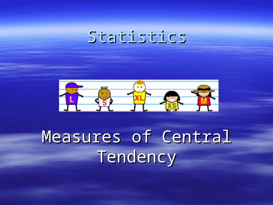
StatisticsStatistics
Measures of Central Measures of Central TendencyTendency
Why Describe Central Tendency?Why Describe Central Tendency?
• Data often cluster around a central value that Data often cluster around a central value that lies between the two extremes. This single lies between the two extremes. This single number can describe the value of scores in number can describe the value of scores in the entire data set.the entire data set.
• There are three measures of central There are three measures of central tendency.tendency.
1) Mean1) Mean
2) Median2) Median
3) Mode 3) Mode
Measures of central tendency are scores Measures of central tendency are scores that represent the center of the that represent the center of the distribution.distribution.
Three of the most common measures of Three of the most common measures of central tendency are:central tendency are:– MeanMean– MedianMedian– ModeMode
MeanMean
The most commonly used measure of central The most commonly used measure of central tendencytendency
When people ask about the “average” of a group of When people ask about the “average” of a group of scores, they usually are referring to the mean.scores, they usually are referring to the mean.
The mean is the sum of all the scores in the The mean is the sum of all the scores in the distribution divided by the total scores (the distribution divided by the total scores (the mathematical average). mathematical average).
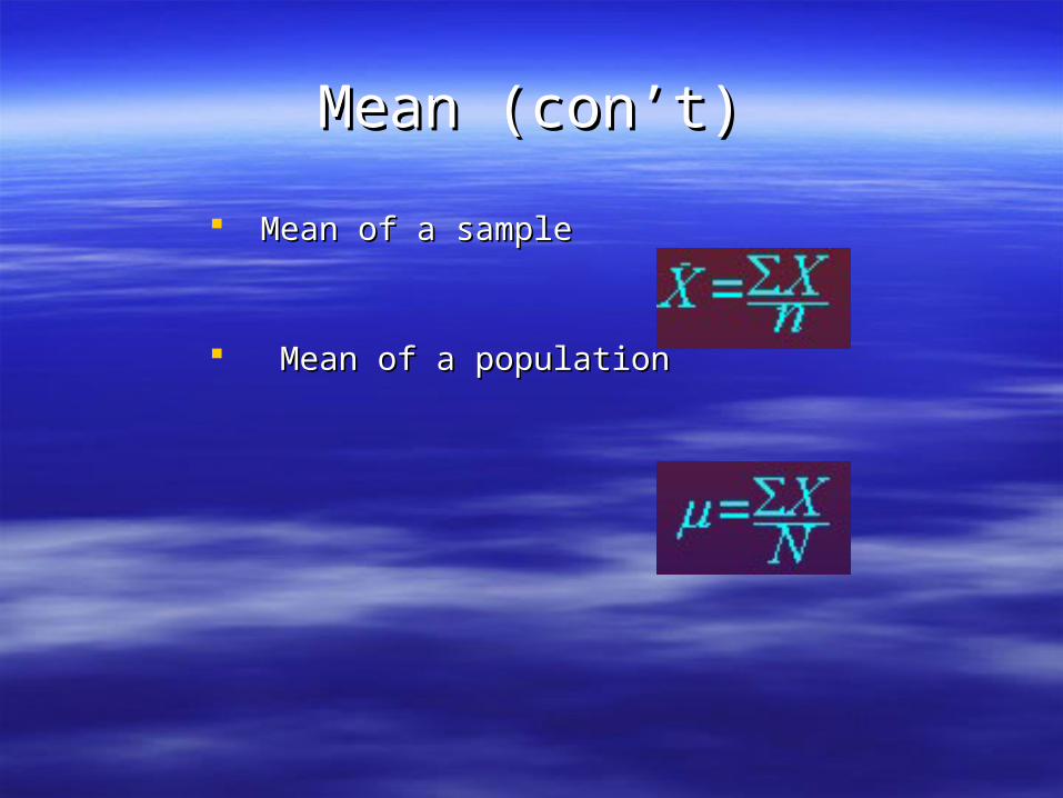
Mean (con’t)Mean (con’t)
Mean of a sampleMean of a sample
Mean of a populationMean of a population
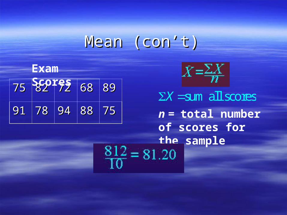
Mean (con’t)Mean (con’t)
7575 8282 7272 6868 8989
9191 7878 9494 8888 7575
Exam Scores
sum all scoresX n = total number of scores for the sample
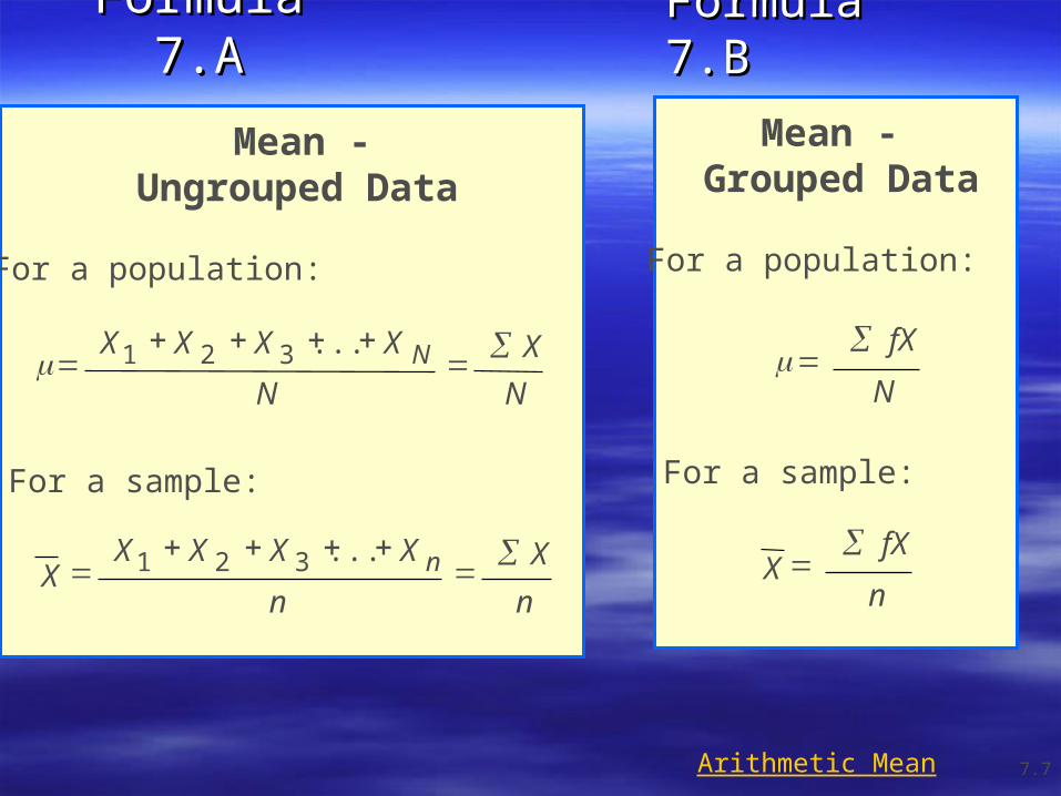
Formula 7.AFormula 7.A
Arithmetic Mean
Mean - Ungrouped Data
For a population:
N
X
N
XXXX N
...321
For a sample:
n
X
n
XXXXX n
...321
Mean - Grouped Data
For a population:
N
fX
For a sample:
n
fXX
Formula 7.BFormula 7.B
7.7
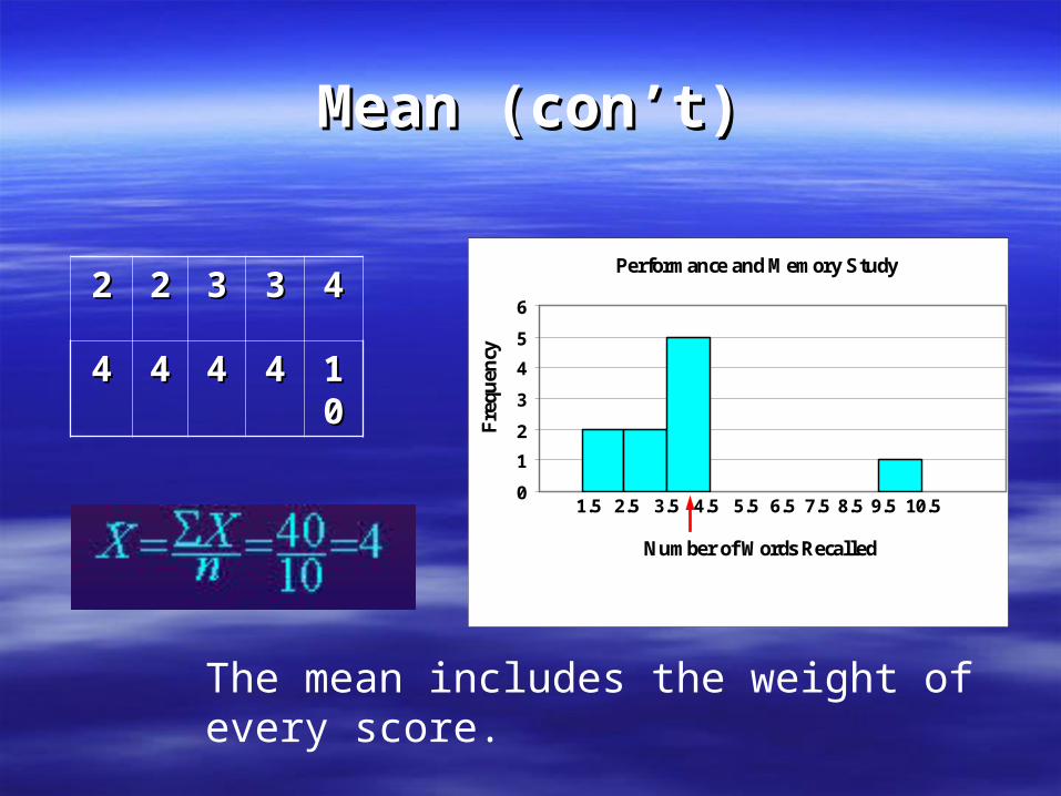
Mean (con’t)Mean (con’t)
Performance and Memory Study
10.59.58.57.56.55.54.53.52.51.50
1
2
3
4
5
6
Number of Words Recalled
Fre
quen
cy
22 22 33 33 44
44 44 44 44 1100
The mean includes the weight of every score.
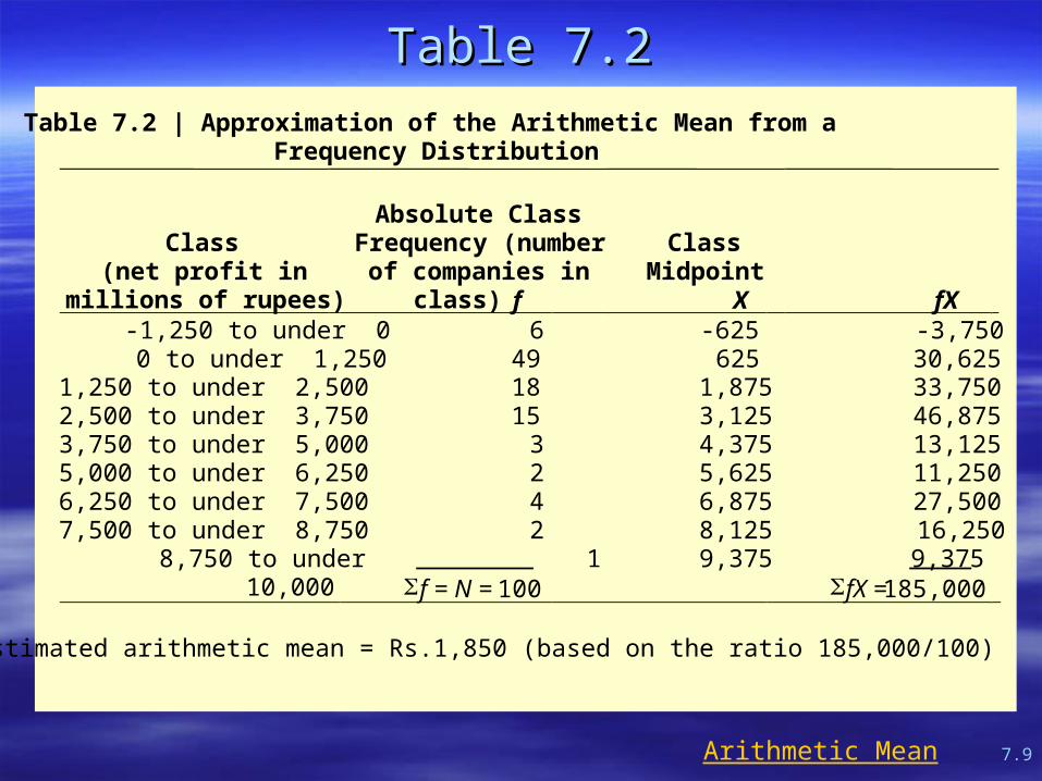
Table 7.2Table 7.2
Arithmetic Mean
Table 7.2 | Approximation of the Arithmetic Mean from a Frequency Distribution
Class(net profit in
millions of rupees)
Absolute ClassFrequency (number
of companies inclass) f
ClassMidpoint X fX
-1,250 to under 0 0 to under 1,250
1,250 to under 2,5002,500 to under 3,7503,750 to under 5,0005,000 to under 6,2506,250 to under 7,5007,500 to under 8,750
8,750 to under10,000
6491815 3 2 4 2
1f = N = 100
-625 625
1,875 3,125 4,375 5,625 6,875 8,125 9,375
-3,750 30,625 33,750 46,875 13,125 11,250 27,500
16,2509,375
fX =185,000
Estimated arithmetic mean = Rs.1,850 (based on the ratio 185,000/100)
7.9
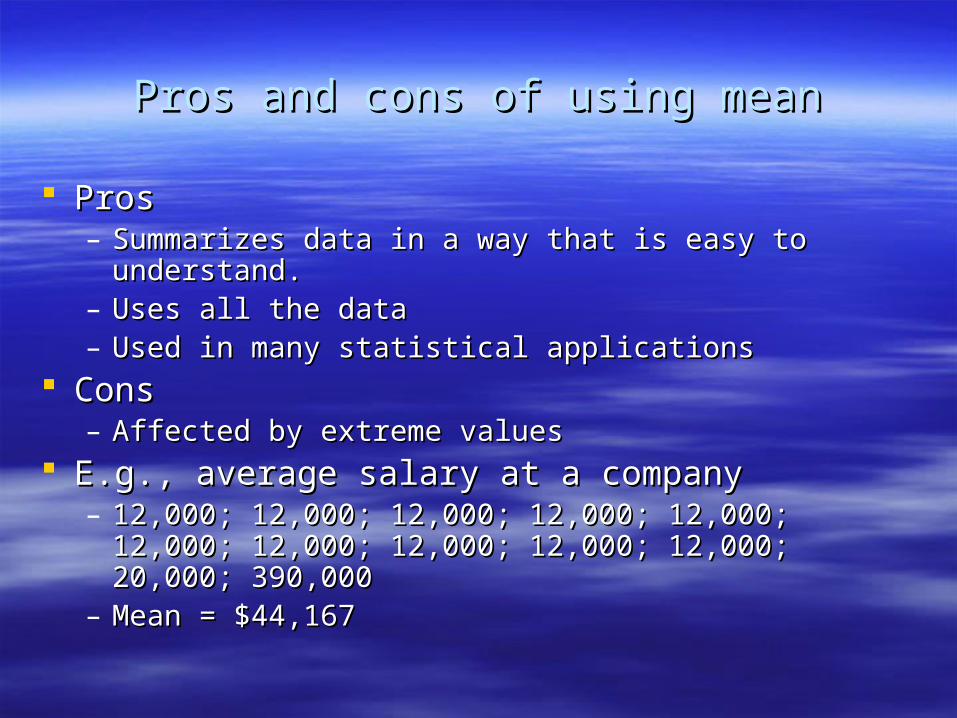
Pros and cons of using meanPros and cons of using mean
ProsPros– Summarizes data in a way that is easy to understand.Summarizes data in a way that is easy to understand.– Uses all the data Uses all the data – Used in many statistical applicationsUsed in many statistical applications
Cons Cons – Affected by extreme valuesAffected by extreme values
E.g., average salary at a companyE.g., average salary at a company– 12,000; 12,000; 12,000; 12,000; 12,000; 12,000; 12,000; 12,000; 12,000; 12,000; 12,000; 12,000;
12,000; 12,000; 12,000; 12,000; 20,000; 390,00012,000; 12,000; 12,000; 12,000; 20,000; 390,000– Mean = $44,167Mean = $44,167
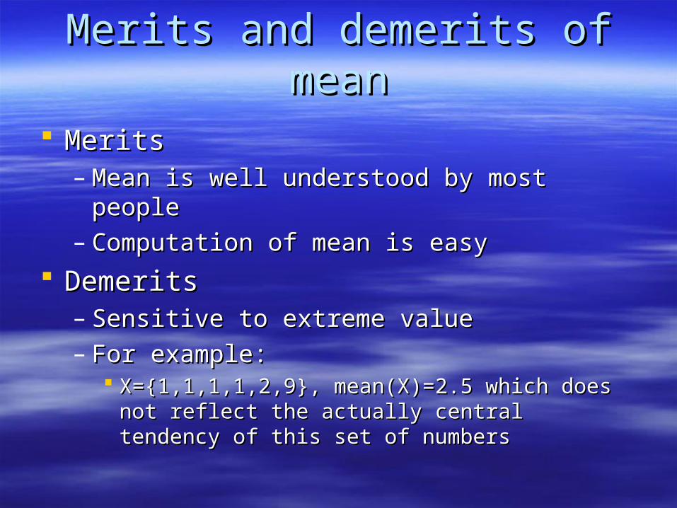
Merits and demerits of meanMerits and demerits of mean MeritsMerits
– Mean is well understood by most peopleMean is well understood by most people– Computation of mean is easyComputation of mean is easy
DemeritsDemerits– Sensitive to extreme valueSensitive to extreme value– For example:For example:
X={1,1,1,1,2,9}, mean(X)=2.5 which does not X={1,1,1,1,2,9}, mean(X)=2.5 which does not reflect the actually central tendency of this set of reflect the actually central tendency of this set of numbersnumbers
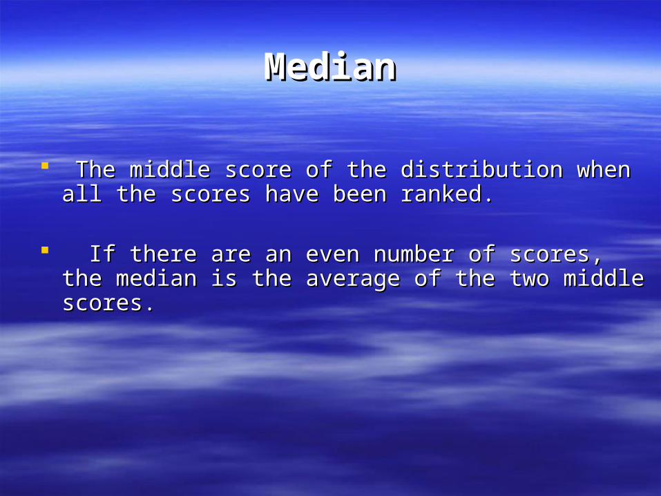
MedianMedian
The middle score of the distribution when all the The middle score of the distribution when all the scores have been ranked.scores have been ranked.
If there are an even number of scores, the median If there are an even number of scores, the median is the average of the two middle scores.is the average of the two middle scores.
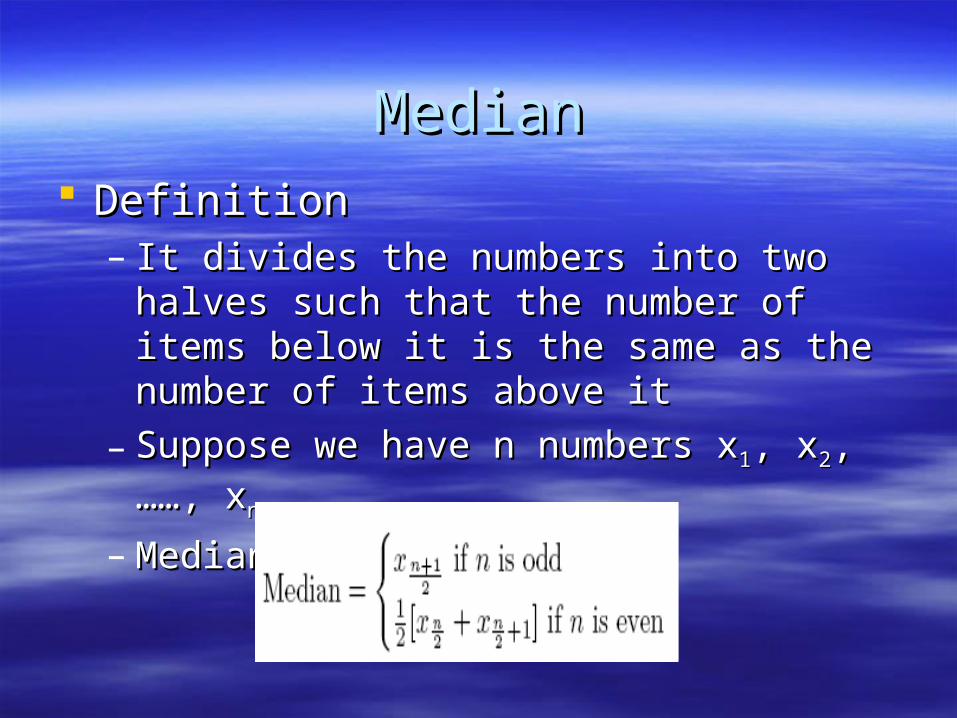
MedianMedian DefinitionDefinition
– It divides the numbers into two halves such It divides the numbers into two halves such that the number of items below it is the same that the number of items below it is the same as the number of items above itas the number of items above it
– Suppose we have n numbers xSuppose we have n numbers x11, x, x22, ……, x, ……, xnn. .
– Median is defined asMedian is defined as
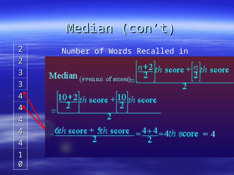
Median (con’t)Median (con’t)
22
22
33
33
44
44
44
44
44
1010
Number of Words Recalled in Performance Study
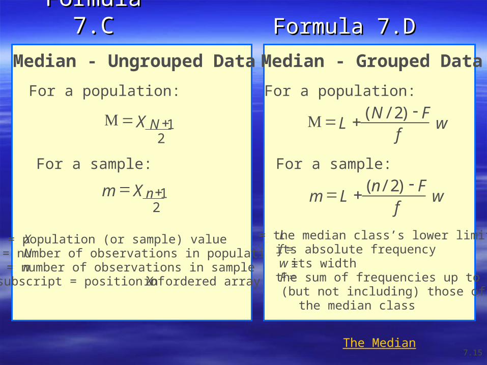
Formula 7.CFormula 7.C
The Median
Median - Ungrouped Data
For a population:
For a sample:
21 NX
21 nXm
X = population (or sample) valueN = number of observations in populationn = number of observations in samplesubscript = position of X in ordered array
Median - Grouped Data
For a population:
For a sample:
wf
FNL
)2/(
wf
FnLm
)2/(
L = the median class’s lower limitf = its absolute frequencyw = its widthF = the sum of frequencies up to (but not including) those of the median class
Formula 7.DFormula 7.D
7.15
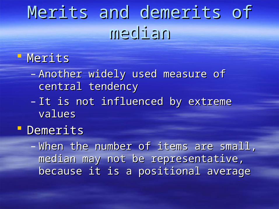
Merits and demerits of medianMerits and demerits of median MeritsMerits
– Another widely used measure of central Another widely used measure of central tendencytendency
– It is not influenced by extreme valuesIt is not influenced by extreme values
DemeritsDemerits– When the number of items are small, median When the number of items are small, median
may not be representative, because it is a may not be representative, because it is a positional averagepositional average
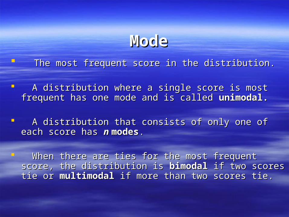
ModeMode The most frequent score in the distribution.The most frequent score in the distribution.
A distribution where a single score is most frequent has one A distribution where a single score is most frequent has one mode and is called mode and is called unimodal.unimodal.
A distribution that consists of only one of each score has A distribution that consists of only one of each score has n n modesmodes..
When there are ties for the most frequent score, the When there are ties for the most frequent score, the distribution is distribution is bimodalbimodal if two scores tie or if two scores tie or multimodalmultimodal if more if more than two scores tie.than two scores tie.
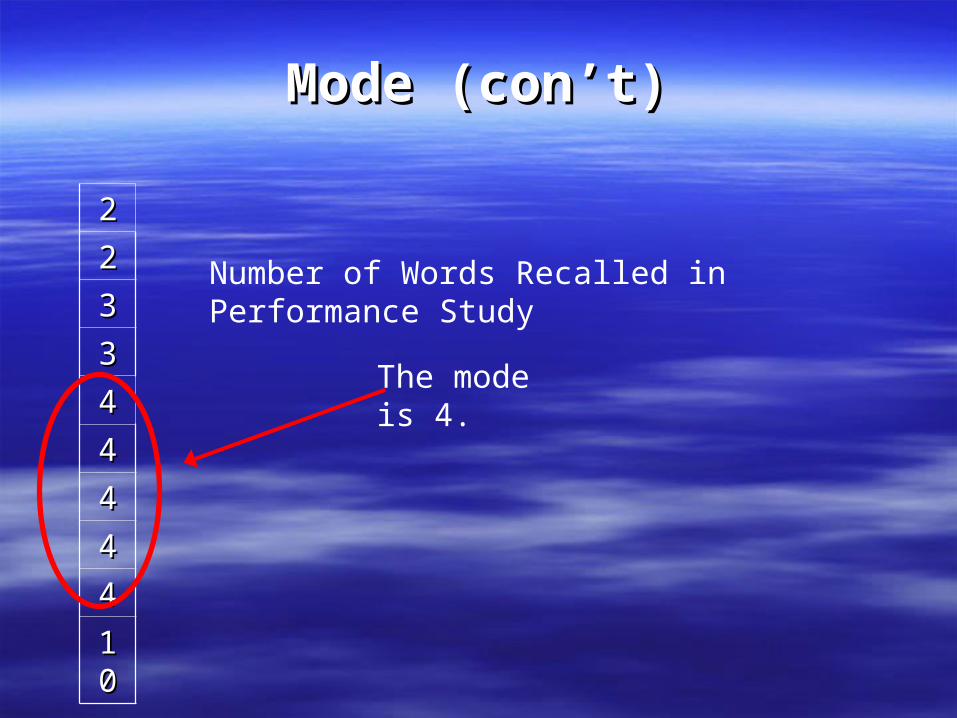
Mode (con’t)Mode (con’t)
22
22
33
33
44
44
44
44
44
1010
Number of Words Recalled in Performance Study
The mode is 4.
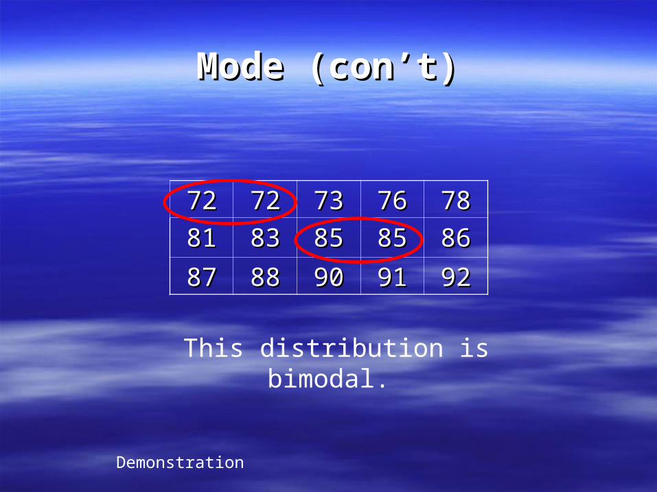
Mode (con’t)Mode (con’t)
7272 7272 7373 7676 7878
8181 8383 8585 8585 8686
8787 8888 9090 9191 9292
This distribution is bimodal.
Demonstration
CalculationsCalculations Key: dependent measure is reaction timeKey: dependent measure is reaction time
– Time it takes to say the colorTime it takes to say the color
Determine the mean, median, and mode Determine the mean, median, and mode of the datasets in the handout.of the datasets in the handout.
Shape of the DistributionShape of the Distribution
Skew refers to the general shape of a distribution when it is graphed.
Symmetrical = zero skew
Scores clustered on the high or low end of a distribution = skewed distribution
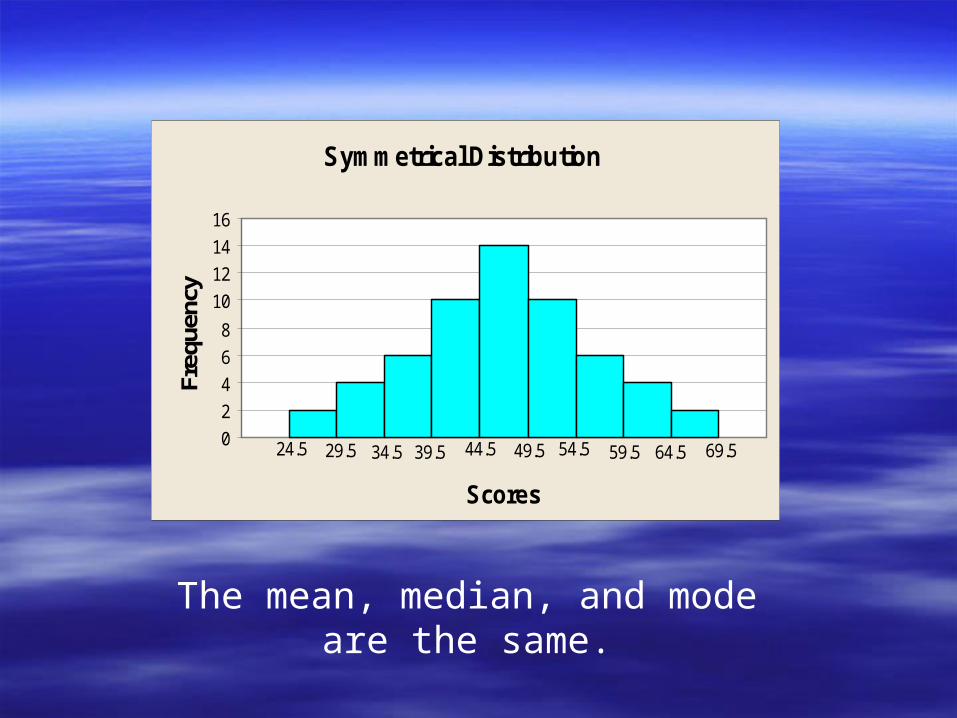
Symmetrical Distribution
24.5 29.5 34.5 39.5 44.5 49.5 54.5 59.5 64.5 69.50
2
4
6
8
10
12
14
16
Scores
Freq
uenc
y
The mean, median, and mode are the same.
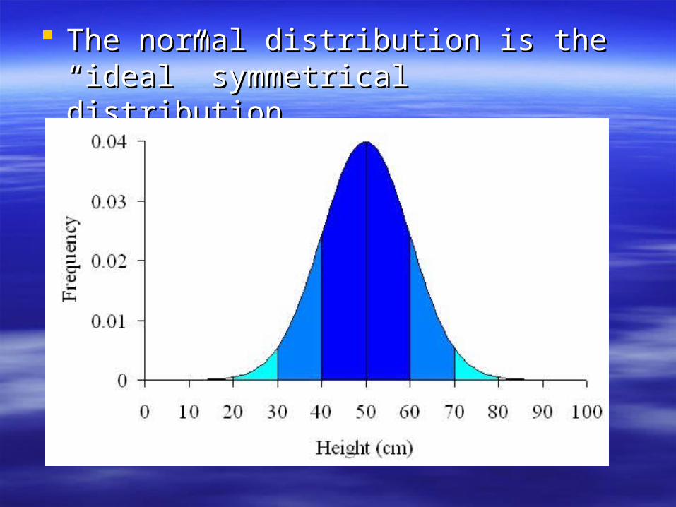
The normal distribution is the “ideal” The normal distribution is the “ideal” symmetrical distributionsymmetrical distribution
Distributions that are skewed have one Distributions that are skewed have one side of the distribution where the data side of the distribution where the data
frequency tapers offfrequency tapers off
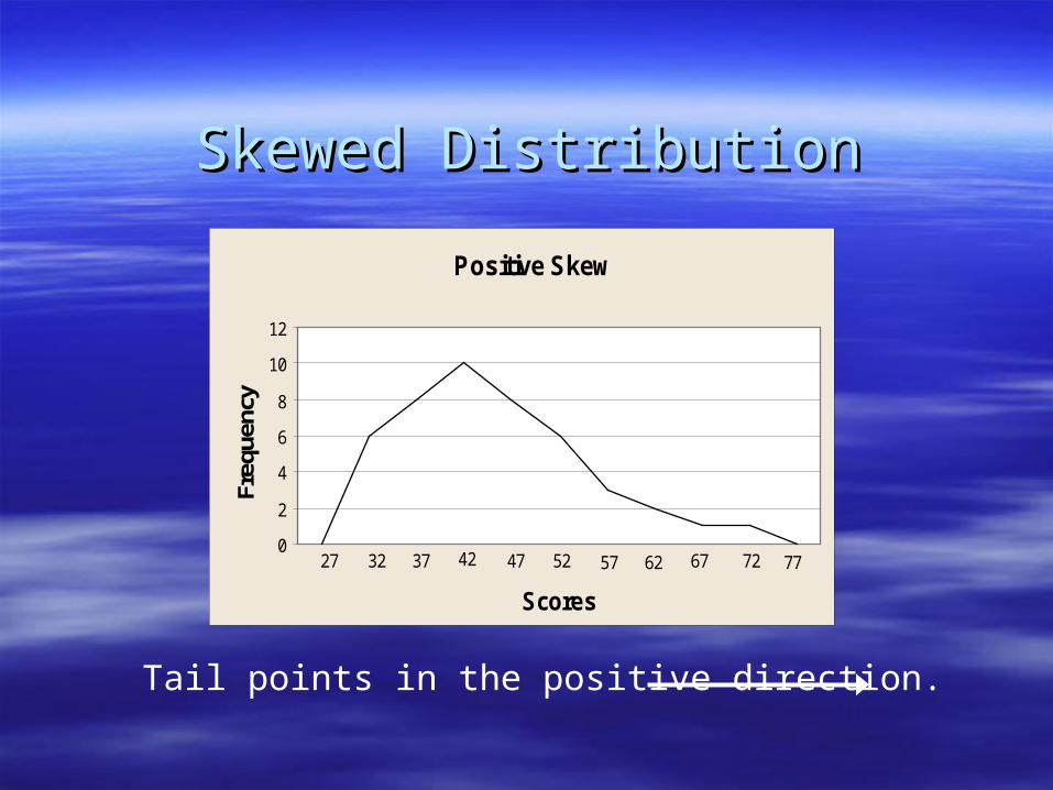
Skewed DistributionSkewed Distribution
Positive Skew
27 32 37 42 47 52 57 62 67 72 770
2
4
6
8
10
12
Scores
Freq
uenc
y
Tail points in the positive direction.
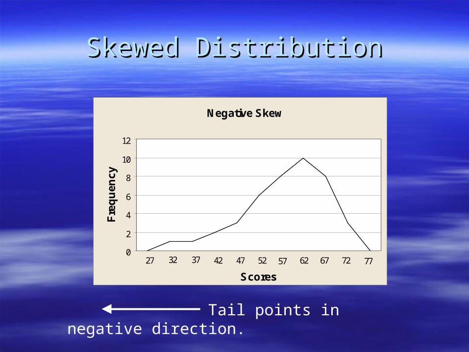
Skewed DistributionSkewed Distribution
Negative Skew
27 32 37 42 47 52 57 62 67 72 770
2
4
6
8
10
12
Scores
Fre
qu
en
cy
Tail points in negative direction.
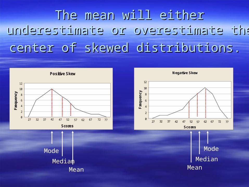
The mean will either underestimate or The mean will either underestimate or overestimate the center of skewed overestimate the center of skewed
distributions.distributions. Positive Skew
27 32 37 42 47 52 57 62 67 72 770
2
4
6
8
10
12
Scores
Freq
uen
cy
Negative Skew
27 32 37 42 47 52 57 62 67 72 770
2
4
6
8
10
12
Scores
Fre
qu
en
cy
Mode
MedianMean
Mode
MeanMedian
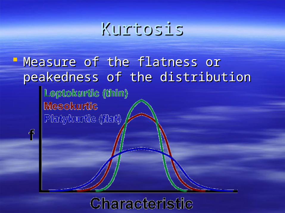
KurtosisKurtosis
Measure of the flatness or peakedness of Measure of the flatness or peakedness of the distributionthe distribution
Measures of LocationMeasures of Location
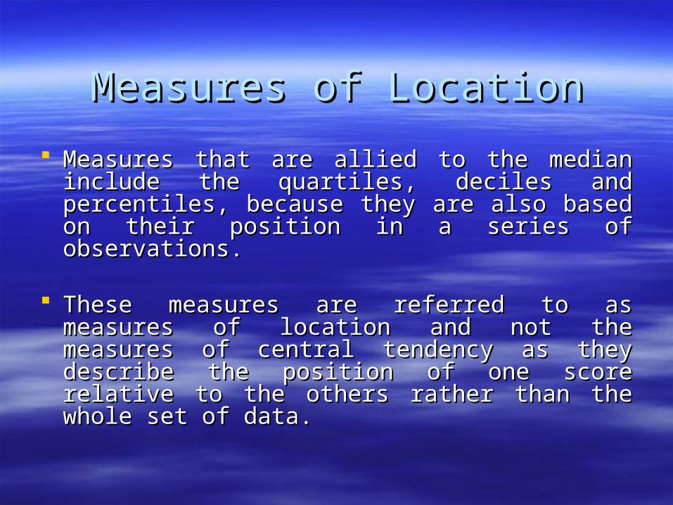
Measures that are allied to the median include Measures that are allied to the median include the quartiles, deciles and percentiles, because the quartiles, deciles and percentiles, because they are also based on their position in a series they are also based on their position in a series of observations. of observations.
These measures are referred to as measures of These measures are referred to as measures of location and not the measures of central location and not the measures of central tendency as they describe the position of one tendency as they describe the position of one score relative to the others rather than the whole score relative to the others rather than the whole set of data.set of data.
Measures of LocationMeasures of Location
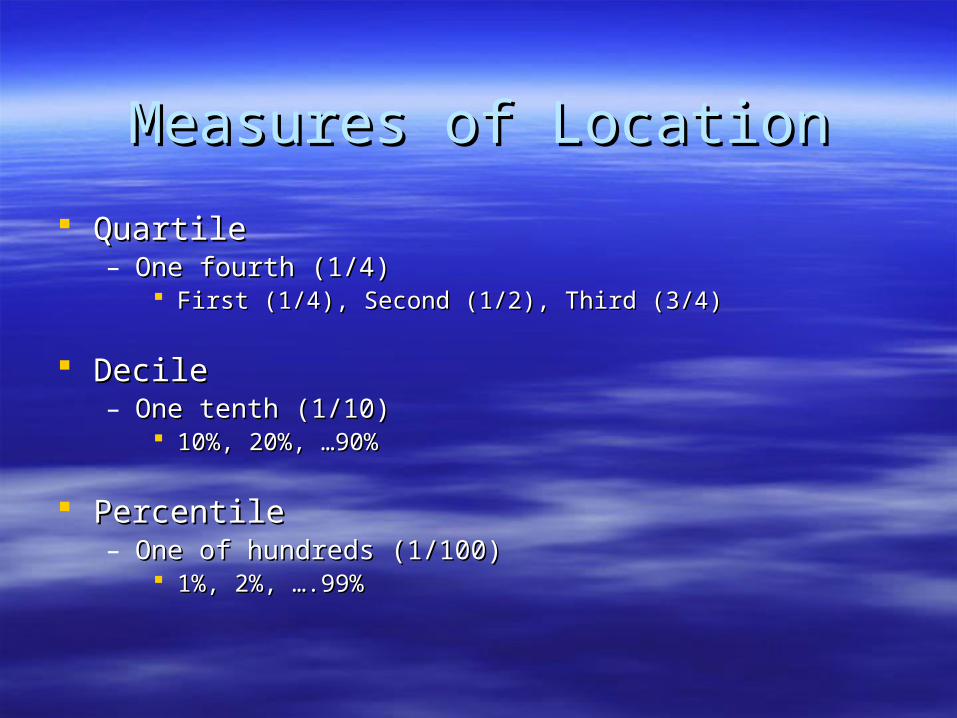
QuartileQuartile– One fourth (1/4)One fourth (1/4)
First (1/4), Second (1/2), Third (3/4) First (1/4), Second (1/2), Third (3/4)
DecileDecile– One tenth (1/10)One tenth (1/10)
10%, 20%, …90%10%, 20%, …90%
Percentile Percentile – One of hundreds (1/100)One of hundreds (1/100)
1%, 2%, ….99%1%, 2%, ….99%
QuartilesQuartiles
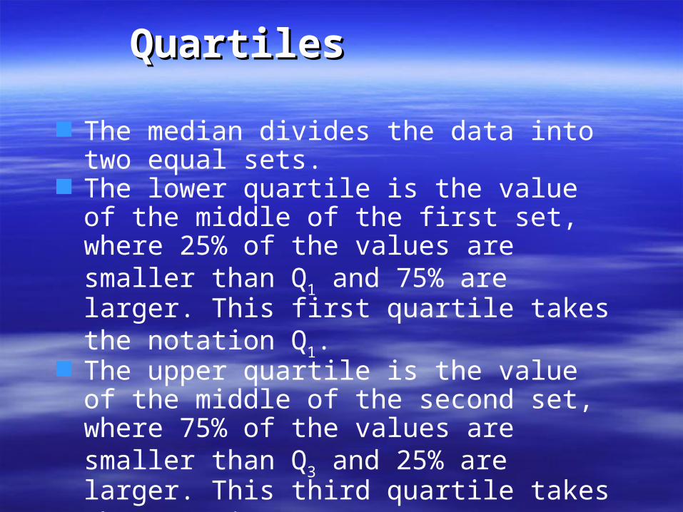
The median divides the data into two equal sets.
The lower quartile is the value of the middle of the first set, where 25% of the values are smaller than Q1 and 75% are larger. This first quartile takes the notation Q1.
The upper quartile is the value of the middle of the second set, where 75% of the values are smaller than Q3 and 25% are larger. This third quartile takes the notation Q3.
QuartilesQuartiles
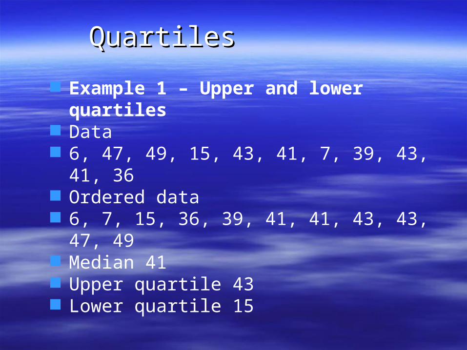
Example 1 – Upper and lower quartiles Data 6, 47, 49, 15, 43, 41, 7, 39, 43, 41, 36 Ordered data 6, 7, 15, 36, 39, 41, 41, 43, 43, 47, 49 Median 41 Upper quartile 43 Lower quartile 15
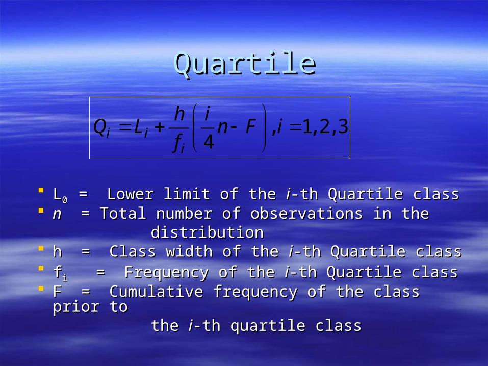
QuartileQuartile
LL0 0 = Lower limit of the = Lower limit of the ii-th Quartile class-th Quartile class nn = Total number of observations in the = Total number of observations in the distributiondistribution h = Class width of the h = Class width of the ii-th Quartile class-th Quartile class ffii = Frequency of the = Frequency of the ii-th Quartile class-th Quartile class F = Cumulative frequency of the class prior to F = Cumulative frequency of the class prior to the the ii-th quartile class-th quartile class
3,2,1,4
iFn
i
f
hLQ
iii
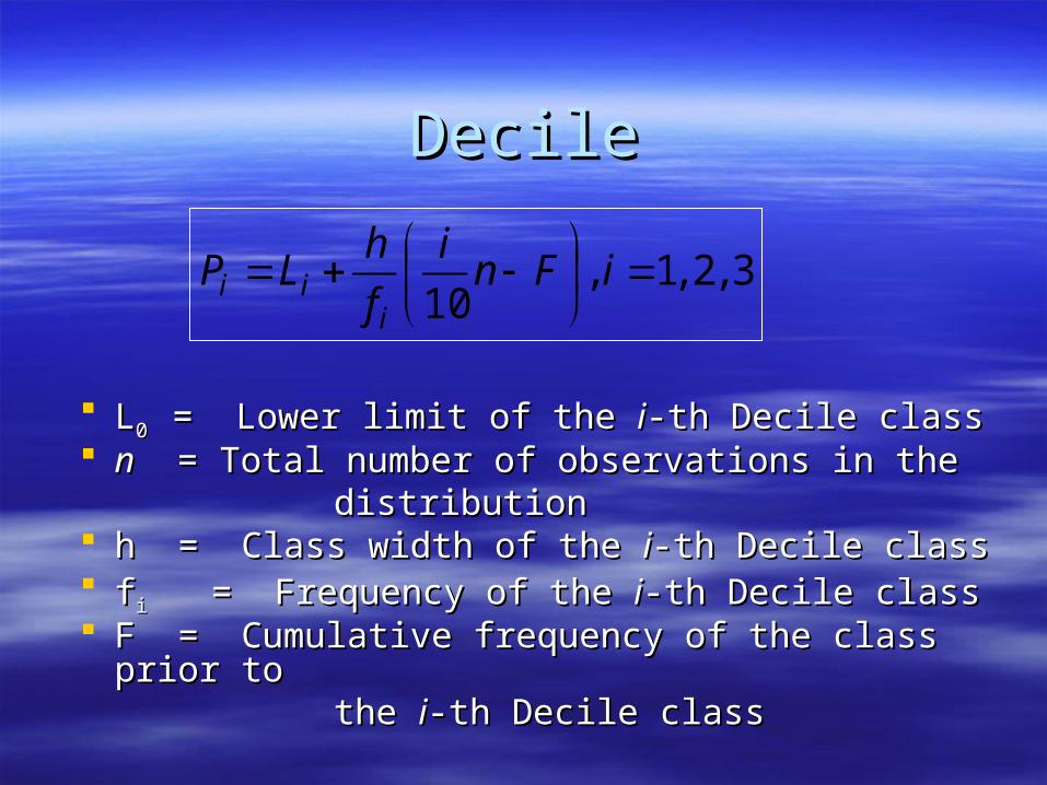
DecileDecile
LL0 0 = Lower limit of the = Lower limit of the ii-th Decile class-th Decile class nn = Total number of observations in the = Total number of observations in the distributiondistribution h = Class width of the h = Class width of the ii-th Decile class-th Decile class ffii = Frequency of the = Frequency of the ii-th Decile class-th Decile class F = Cumulative frequency of the class prior to F = Cumulative frequency of the class prior to the the ii-th Decile class-th Decile class
3,2,1,10
iFn
i
f
hLP
iii
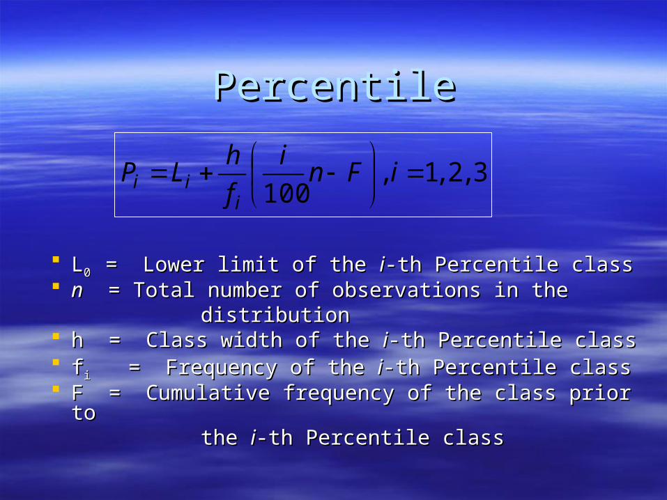
PercentilePercentile
LL0 0 = Lower limit of the = Lower limit of the ii-th Percentile class-th Percentile class nn = Total number of observations in the = Total number of observations in the distributiondistribution h = Class width of the h = Class width of the ii-th Percentile class-th Percentile class ffii = Frequency of the = Frequency of the ii-th Percentile class-th Percentile class F = Cumulative frequency of the class prior to F = Cumulative frequency of the class prior to the the ii-th Percentile class-th Percentile class
3,2,1,100
iFn
i
f
hLP
iii
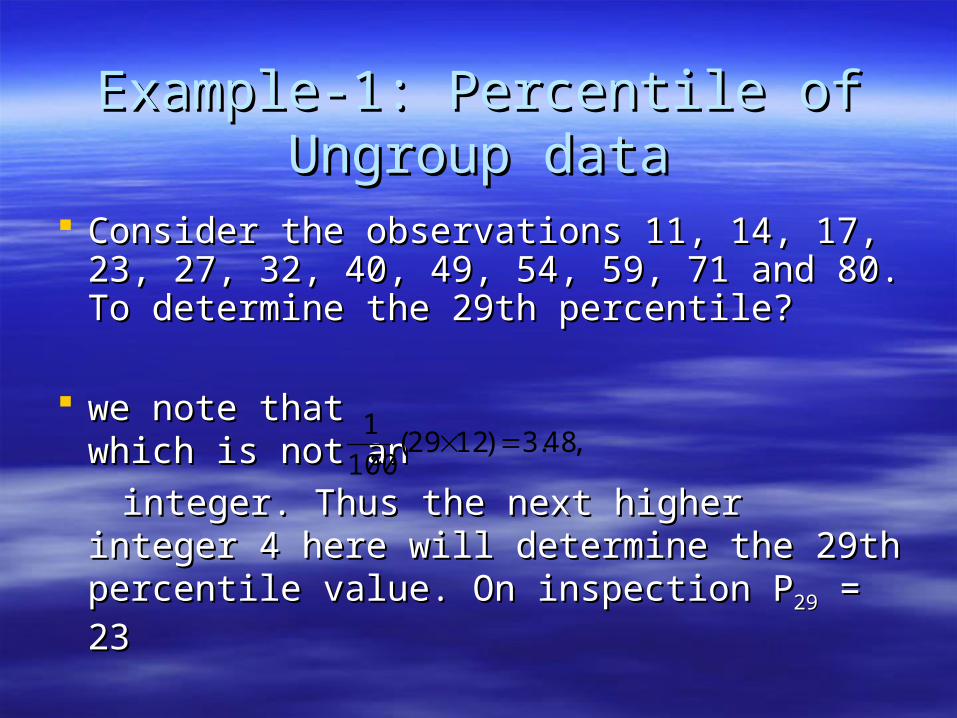
Example-1: Percentile of Ungroup Example-1: Percentile of Ungroup datadata
Consider the observations 11, 14, 17, 23, Consider the observations 11, 14, 17, 23, 27, 32, 40, 49, 54, 59, 71 and 80. To 27, 32, 40, 49, 54, 59, 71 and 80. To determine the 29th percentile? determine the 29th percentile?
we note that which is not an we note that which is not an
integer. Thus the next higher integer 4 here integer. Thus the next higher integer 4 here will determine the 29th percentile value. will determine the 29th percentile value. On inspection POn inspection P2929 = 23 = 23
,48.3)1229(100
1
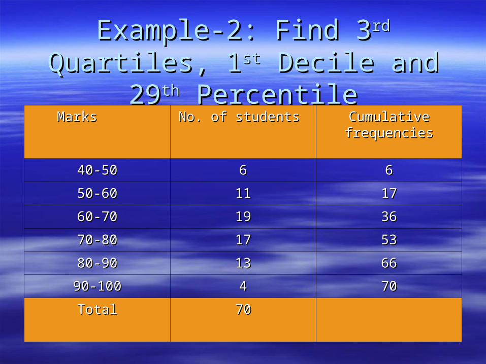
Example-2: Find 3Example-2: Find 3rdrd Quartiles, 1 Quartiles, 1stst Decile and 29Decile and 29thth Percentile Percentile
Marks Marks
No. of students No. of students Cumulative Cumulative frequenciesfrequencies
40-5040-50 66 66
50-6050-60 1111 1717
60-7060-70 1919 3636
70-8070-80 1717 5353
80-9080-90 1313 6666
90-10090-100 44 7070
TotalTotal 7070
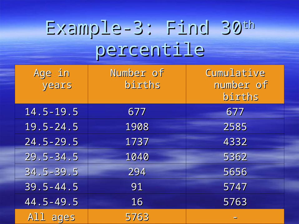
Example-3: Find 30Example-3: Find 30thth percentile percentile
Age in yearsAge in years Number of birthsNumber of births Cumulative number Cumulative number of birthsof births
14.5-19.514.5-19.5 677677 677677
19.5-24.519.5-24.5 19081908 25852585
24.5-29.524.5-29.5 17371737 43324332
29.5-34.529.5-34.5 10401040 53625362
34.5-39.534.5-39.5 294294 56565656
39.5-44.539.5-44.5 9191 57475747
44.5-49.544.5-49.5 1616 57635763
All agesAll ages 57635763 --
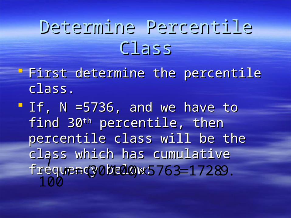
Determine Percentile ClassDetermine Percentile Class
First determine the percentile class.First determine the percentile class. If, N =5736, and we have to find 30If, N =5736, and we have to find 30thth
percentile, then percentile class will be the percentile, then percentile class will be the class which has cumulative frequency class which has cumulative frequency below: below:
.9.17285763)100/30(100
ni
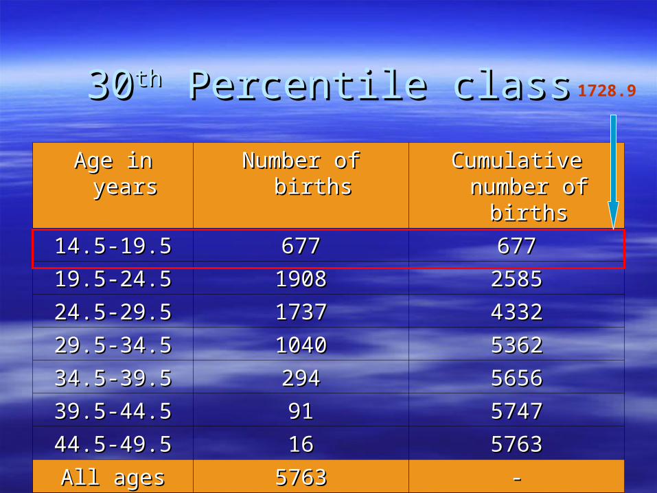
3030thth Percentile class Percentile class
Age in yearsAge in years Number of birthsNumber of births Cumulative number Cumulative number of birthsof births
14.5-19.514.5-19.5 677677 677677
19.5-24.519.5-24.5 19081908 25852585
24.5-29.524.5-29.5 17371737 43324332
29.5-34.529.5-34.5 10401040 53625362
34.5-39.534.5-39.5 294294 56565656
39.5-44.539.5-44.5 9191 57475747
44.5-49.544.5-49.5 1616 57635763
All agesAll ages 57635763 --
1728.9
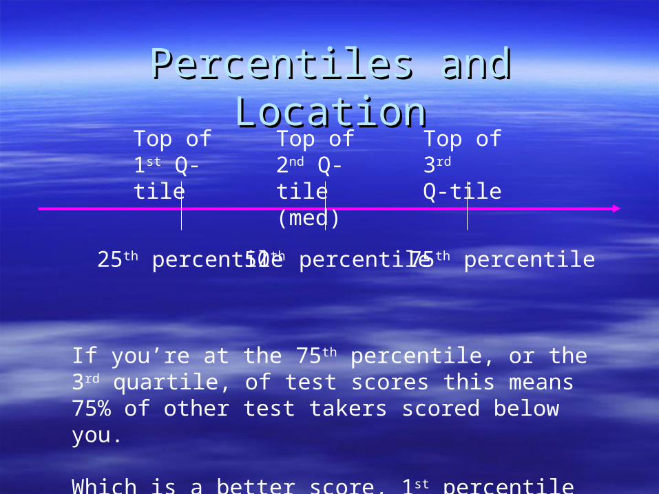
Percentiles and LocationPercentiles and LocationTop of 1st Q-tile
Top of 2nd Q-tile (med)
Top of 3rd
Q-tile
25th percentile 50th percentile 75th percentile
If you’re at the 75th percentile, or the 3rd quartile, of test scores this means 75% of other test takers scored below you.
Which is a better score, 1st percentile or 99th percentile?
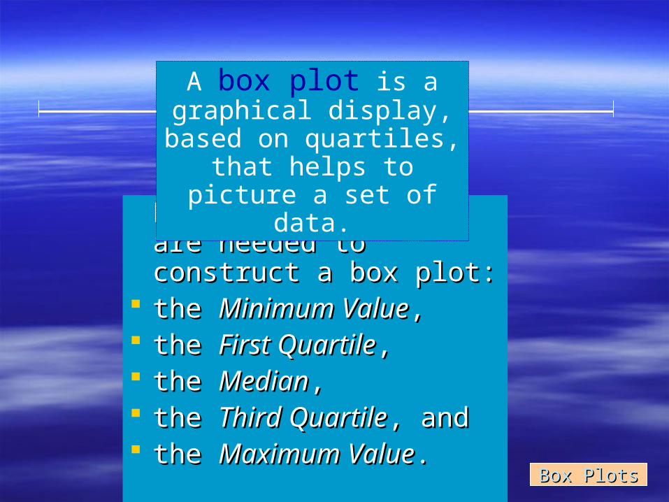
Box PlotsBox Plots
Five pieces of data are Five pieces of data are needed to construct a box needed to construct a box plot: plot:
the the Minimum ValueMinimum Value,, the the First QuartileFirst Quartile,, the the MedianMedian,, the the Third QuartileThird Quartile, and, and the the Maximum ValueMaximum Value..
A box plot is a graphical display, based on quartiles, that helps to picture a set of
data.
Example 4Example 4
Based on a sample of 20 deliveries,
Buddy’s Pizza determined the following information. The
minimum delivery time was 13 minutes and the maximum 30
minutes. The first quartile was 15 minutes, the median 18
minutes, and the third quartile 22 minutes. Develop a box plot
for the delivery times.
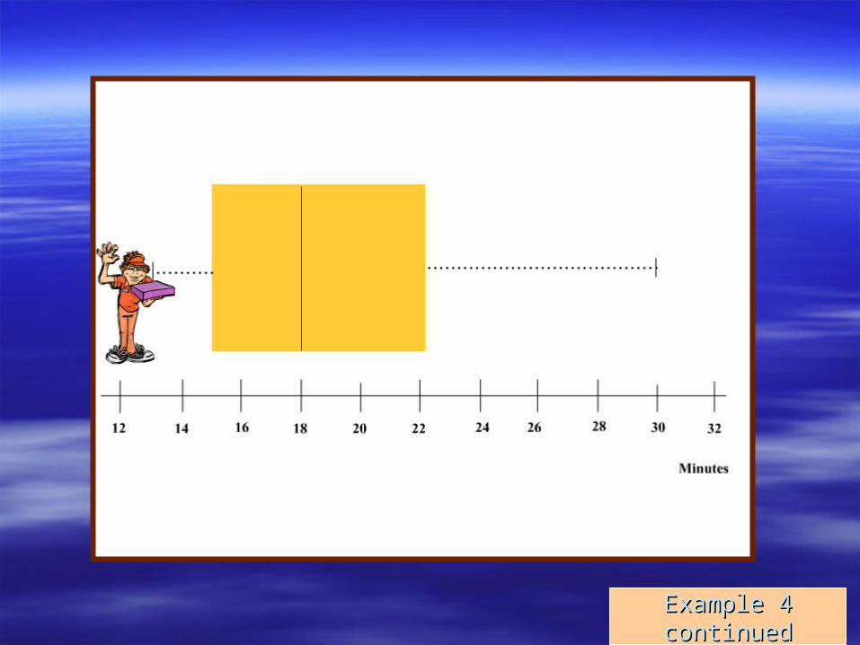
Example 4 Example 4 continuedcontinued