Statistics II: An Overview of Statistics

Outline for Statistics II Lecture:

• SPSS Syntax – Some examples.

• Normal Distribution Curve.

• Sampling Distribution

• Hypothesis Testing

• Type I and Type II Errors

• Linking Z to, alpha, and hypothesis testing.

• Bivariate Measures of Association

• Bivariate Regression/Correlation

The Normal Distribution

The standard normal distribution: a bell-shaped symmetrical distribution having a mean of 0 and a standard deviation of 1.

Z scores.

A z score (or standard score): a transformed score expressed as a deviation from an expected value that has a standard deviation as its unit of measurement. A standard score belonging to the standard normal distribution.

Y-μz = — σ

Sampling Distribution

The Standard Error of the Sampling Distribution.

y--- is the standard error of the sampling distribution of y---, or simply the standard

error of y---.

The standard error describes the spread of the sampling distribution.

It refers to the variability in the value of y--- from sample to sample.

The value of y--- is the number that results from repeatedly selecting samples of

size n from the population, finding y--- for each set of n observations, and calculatingthe standard deviation of the y

--- values.

The symbol y--- (instead of ) and the terminology standard error (instead of

standard deviation) distinguish this measure from the standard deviation of thepopulation distribution.

y

--- = —

y--- = —

n

For a random sample of size n, the standard error of y--- is related to the population

standard deviation by

That is, the spread of the sampling distribution depends on the sample size n, and the spread of the population distribution.

As the sample size n increases the standard error decreases.

The reason for this is that the denominator of the ratio increases as n increases, whereas the numerator is the population standard deviation, which is a constant and is not dependent on the value of n.

Central Limit Theorem

For random sampling, as the sample size n grows, the sampling distribution of approaches a normal distribution.

The approximate normality of the sampling distribution applies no matter what the shape of the population distribution.

Hypothesis Testing

Steps of a Statistical Significance Test.

1. Assumptions

Type of data, form of population, method of sampling, sample size

2. Hypotheses

Null hypothesis, Ho (parameter value for “no effect”)

Alternative hypothesis, Ha (alternative parameter values)

3. Test statistic

Compares point estimate to null hypothesized parameter value

4. P-value

Weight of evidence about Ho; smaller P is more contradictory

5. Conclusion

Report P-value

Formal decision

Alpha or significance levels:

The α - level is a number such that one reject if Ho if the P-value is less than or equal to it.

The α - level is also called the significance level of the test.

The most common α - levels are .05 and .01.

Type I and Type II Errors:

A Type I error occurs when Ho is rejected, even though it is true.

A Type II error occurs when Ho is not rejected, even though it is false.

Decision

Reject Hoo Do not reject Hoo

In reality: Hoo is true Type I error Correct decision

Hoo is false Correct decision Type II error

Using z and the Area Under the Normal Curve to Test for Statistical Significance

Number of tails of test

Proportion UnderCurve (e.g. between and z score on the

standard normaldistribution).

Critical z score

.05 one .45(.50 - .05 = .45)

1.645

.05 two .475(.50 - .025 = .475)

1.96

.01 one .49(.50 - .01 = .49)

2.33

.01 two .495(.50 - .005 = .495)

2.575

Bivariate Statistics

PROPORTIONAL REDUCTION IN ERROR (PRE)

“all good measures of association use a proportionate reduction in error (PRE) approach.

The PRE family of statistics is based on comparing the errors made in predicting the dependent variable with knowledge of the independent variable, to the errors made without information about the independent variable.

In other words, PRE measures indicate how knowing the values of the independent variable (first variable) increase our ability to accurately predict the dependent variable (second variable).

Error without Error withdecision rule - decision rule

PRE statistic = _____________________________

Error without decision rule

Another way of stating this is:

E1 - E2PRE value = _____

E1

Where E1 = number of errors made by the first prediction method.

E2 = number of errors made by the second prediction method.

• PRE measures are more versatile and more informative than are the chi-square-based measures.

• All PRE measures are normed; they use a standardized scale where the value 0 means there is no association and 1 means there is perfect association.

• Any value between these extremes indicates the relative degree of association in a ratio comparison sense. E.g., a PRE measure with a value of .50 represents an association that is twice as strong as one that has a PRE value of .25.

• The number of cases, the table size, and the variables being measured do not interfere with the interpretation that can be given to them.

Chi Square

The Chi-square test examines whether two nominal variables are associated.

It is NOT a PRE measure.

The chi-square test is based on a comparison between the frequencies that are observed in the cells of a cross-classification table and those that we would expect to observe if the null hypothesis were true.

The hypotheses for the chi-square are:

Ho: the variables are statistically independent.

Ha: the variables are statistically dependent.

Goodman and Kruska’s Gamma (G)

A measure of association for data grouped in ordered categories.

G is a PRE measure.

G compares two measures of a prediction:

1st it randomly predicts all untied scores to be either in agreement or disagreement.

2nd it predicts all untied pairs to be of the same type.

Agreement or disagreement is determined by the direction of the bivariate distribution.

For a positive pattern we expect untied pairs to be in agreement

For a negative pattern we expect untied pairs to be in disagreement.

Pa: we find the number of agreement pairs by multiplying the frequency for each cell by the sum of the frequencies from all cells that are both to the right and below it.

Pd: is found by multiplying the frequency for each cell in the table by the sum of the frequencies from all cells that are both to the left and below it.

Bivariate Regression and Correlation

BIVARIATE REGRESSION AND CORRELATION

WHY AND WHEN TO USE REGRESSION/CORRELATION?

WHAT DOES REGRESSION/CORRELATION MEAN?

You should be able to interpret:

The least squares equation.

R2 and Adjusted R2

F and significance.

The unstandardized regression coefficient.

The standardized regression coefficient.

t and significance.

The 95% confidence interval.

A graph of the regression line.

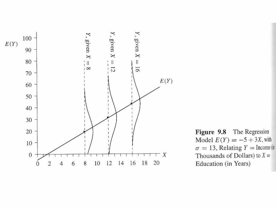
ASSUMPTIONS UNDERLYING REGRESSION/CORRELATION

NORMALITY OF VARIANCE IN Y FOR EACH VALUE OF X

For any fixed value of the independent variable X, the distribution of the dependent variable Y is normal.

NORMALITY OF VARIANCE FOR THE ERROR TERM

The error term is normally distributed. (Many authors argue that this is more important than normality in the distribution of Y).

THE INDEPENDENT VARIABLE IS UNCORRELATED WITH THE ERROR TERM

ASSUMPTIONS UNDERLYING REGRESSION/CORRELATION (Continued)

HOMOSCEDASTICITY

It is assumed that there is equal variances for Y, for each fixed value of X.

LINEARITY

The relationship between X and Y is linear.

INDEPENDENCE

The Y’s are statistically independent of each other.