Embed Size (px)
DESCRIPTION
Statistics, project,
Citation preview
SAMPLING TECHNIQUES AND NORMAL DISTRIBUTION

1 STATISTICS & PROBABILITY
Foreword
This hand out contains various lectures on sampling techniques and normal
distribution as well as problems and exercises to guide you in. We hope that the
contents of this hand out will be much of help to your study of statistics.
2 STATISTICS & PROBABILITY
PART 1: SAMPLING TECHNIQUES
In reality there is simply not enough; time, energy, money,
labor/man power, equipment, access to suitable sites to
measure every single item or site within the parent
population or whole sampling frame. Therefore an
appropriate sampling strategy is adopted to obtain a
representative, and statistically valid sample of the whole.
WHAT IS SAMPLING?
A shortcut method for investigating a whole population
Data is gathered on a small part of the whole parent population or
sampling frame, and used to inform what the whole picture is like
CONSIDERATIONS IN SAMPLING
Larger sample sizes are more accurate representations of the whole
The sample size chosen is a balance between obtaining a statistically
valid representation, and the time, energy, money, labor, equipment and
access available
A sampling strategy made with the minimum of bias is the most
statistically valid
Most approaches assume that the parent population has a normal
distribution where most items or individuals clustered close to the mean,
with few extremes
3 STATISTICS & PROBABILITY
WHAT ARE SAMPLING TECHNIQUES?
Sampling techniques are classified as either probability or
nonprobability. In probability samples, each member of the
population has a known non-zero probability of being selected. Probability
methods include random sampling, systematic sampling, and stratified
sampling. In nonprobability sampling, members are selected from the
population in some nonrandom manner. In this part we will be focusing on the
probability types of sampling techniques.
THREE MAIN TYPES OF SAMPLING STRATEGY:
Random
Systematic
Stratified
Within these types, you may then decide on a; point, line, area method.
RANDOM SAMPLING
Least biased of all sampling techniques, there is no
subjectivity - each member of the total population has an
equal chance of being selected
Can be obtained using random number tables
Microsoft Excel has a function to produce random number
4 STATISTICS & PROBABILITY
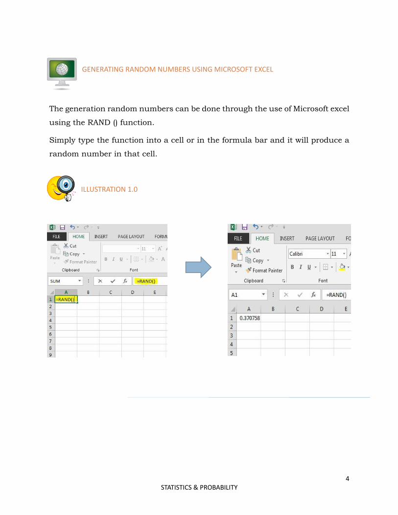
GENERATING RANDOM NUMBERS USING MICROSOFT EXCEL
The generation random numbers can be done through the use of Microsoft excel
using the RAND () function.
Simply type the function into a cell or in the formula bar and it will produce a
random number in that cell.
ILLUSTRATION 1.0
5 STATISTICS & PROBABILITY
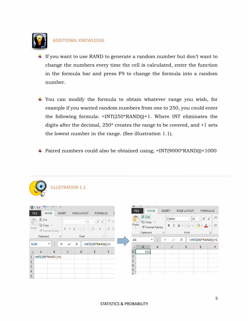
ADDITIONAL KNOWLEDGE
If you want to use RAND to generate a random number but don’t want to
change the numbers every time the cell is calculated, enter the function
in the formula bar and press F9 to change the formula into a random
number.
You can modify the formula to obtain whatever range you wish, for
example if you wanted random numbers from one to 250, you could enter
the following formula: =INT(250*RAND())+1. Where INT eliminates the
digits after the decimal, 250* creates the range to be covered, and +1 sets
the lowest number in the range. (See illustration 1.1).
Paired numbers could also be obtained using; =INT(9000*RAND())+1000
ILLUSTRATION 1.1
6 STATISTICS & PROBABILITY
PRACTICE WHAT YOU LEARNED
Using the RAND function in Microsoft excel generate a random number between the following values:
1. 0 and 90 2. 0 and 20 3. 30 and 200
4. 10 and 30 5. 100 and 900
METHODOLOGIES
Random point sampling
A grid is drawn over a map of the study area
Random number tables are used to obtain coordinates/grid references for
the points
Sampling takes place as feasibly close to these points as possible
Random line sampling
Pairs of coordinates or grid references are obtained using random number
tables, and marked on a map of the study area
These are joined to form lines to be sampled
Random area sampling
Random number tables generate coordinates or grid references which are
used to mark the bottom left (south west) corner of quadrats or grid
squares to be sampled
7 STATISTICS & PROBABILITY
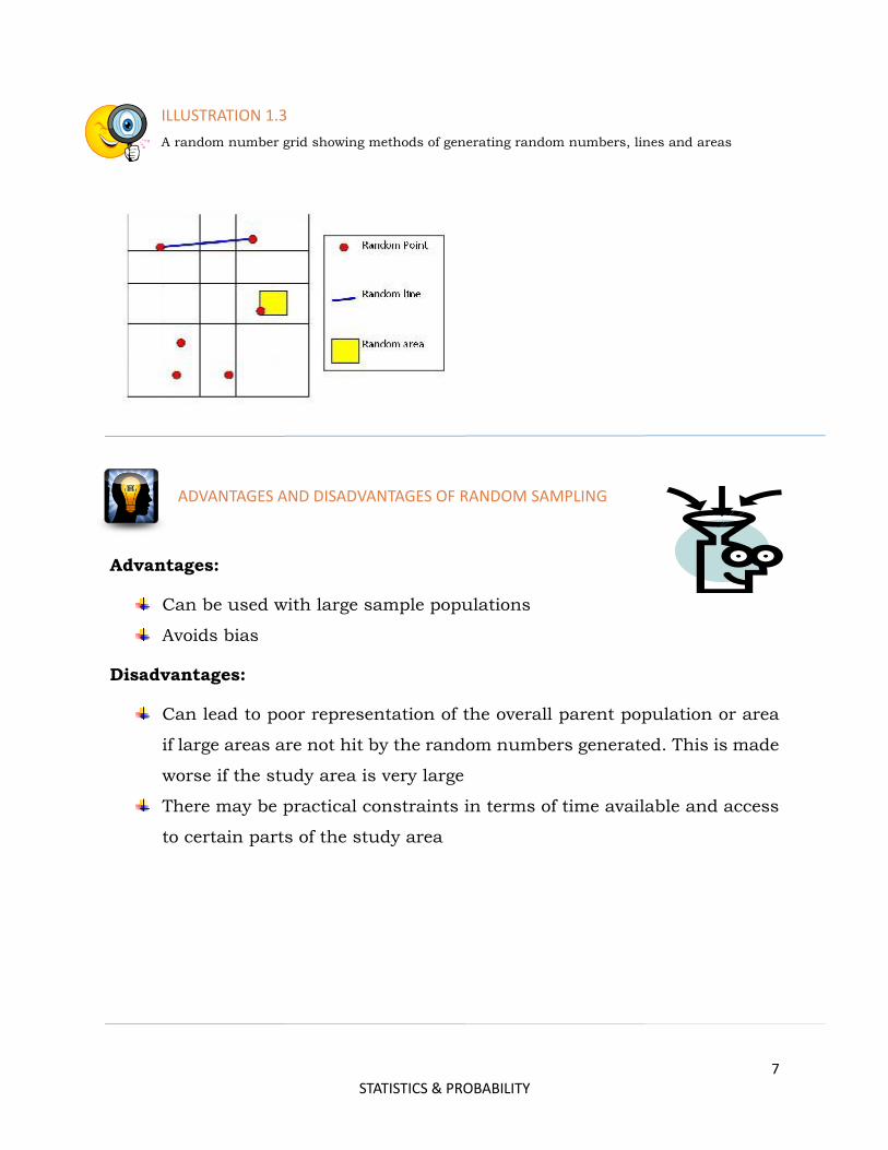
ILLUSTRATION 1.3
A random number grid showing methods of generating random numbers, lines and areas
ADVANTAGES AND DISADVANTAGES OF RANDOM SAMPLING
Advantages:
Can be used with large sample populations
Avoids bias
Disadvantages:
Can lead to poor representation of the overall parent population or area
if large areas are not hit by the random numbers generated. This is made
worse if the study area is very large
There may be practical constraints in terms of time available and access
to certain parts of the study area
8 STATISTICS & PROBABILITY
SYTEMATIC SAMPLING
Samples are chosen in a systematic, or regular way.
They are evenly/regularly distributed in a spatial context, for example
every two meters along a transect line
They can be at equal/regular intervals in a temporal context, for example
every half hour or at set times of the day
They can be regularly numbered, for example every 10th house or person
METHODOLOGIES
A. Systematic point sampling
A grid can be used and the points can be at the intersections of the grid
lines (A), or in the middle of each grid square (B). Sampling is done at the
nearest feasible place. Along a transect line, sampling points for
vegetation/pebble data collection could be identified systematically, for
example every two meters or every 10th pebble.
B. Systematic line sampling
The eastings or northings of the grid on a map can be used to identify
transect lines (C and D) alternatively, along a beach it could be decided
that a transect up the beach will be conducted every 20 meters along the
length of the beach.
C. Systematic area sampling
A ‘pattern' of grid squares to be sampled can be identified using a map of
the study area, for example every second/third grid square down or
across the area (E) - the south west corner will then mark the corner of a
quadrat. Patterns can be any shape or direction as long as they are
regular (F).

9 STATISTICS & PROBABILITY
ILLUSTRATION 1.4
ADVANTAGES AND DISADVANTAGES OF SYSTEMATIC SAMPLING
Advantages:
It is more straight-forward than random sampling
A grid doesn't necessarily have to be used, sampling just has to be at
uniform intervals
A good coverage of the study area can be more easily achieved than using
random sampling
Disadvantages:
It is more biased, as not all members or points have an equal chance of
being selected
It may therefore lead to over or under representation of a particular
pattern
10 STATISTICS & PROBABILITY
STRATIFIED SAMPLING
This method is used when the parent population or sampling
frame is made up of sub-sets of known size. These sub-sets make up different
proportions of the total, and therefore sampling should be stratified to ensure
that results are proportional and representative of the whole.
TYPES OF STRATIFIED SAMPLING
A. Stratified systematic sampling
The population can be divided into known groups, and each group sampled
using a systematic approach. The number sampled in each group should be in
proportion to its known size in the parent population.
For example: the make-up of different social groups in the population of a town
can be obtained, and then the number of questionnaires carried out in different
parts of the town can be stratified in line with this information. A systematic
approach can still be used by asking every fifth person.
B. Stratified random sampling
A wide range of data and fieldwork situations can lend themselves to this
approach - wherever there are two study areas being compared, for example
two woodlands, river catchments, rock types or a population with sub-sets of
known size, for example woodland with distinctly different habitats.
Random point, line or area techniques can be used as long as the number of
measurements taken is in proportion to the size of the whole.
11 STATISTICS & PROBABILITY
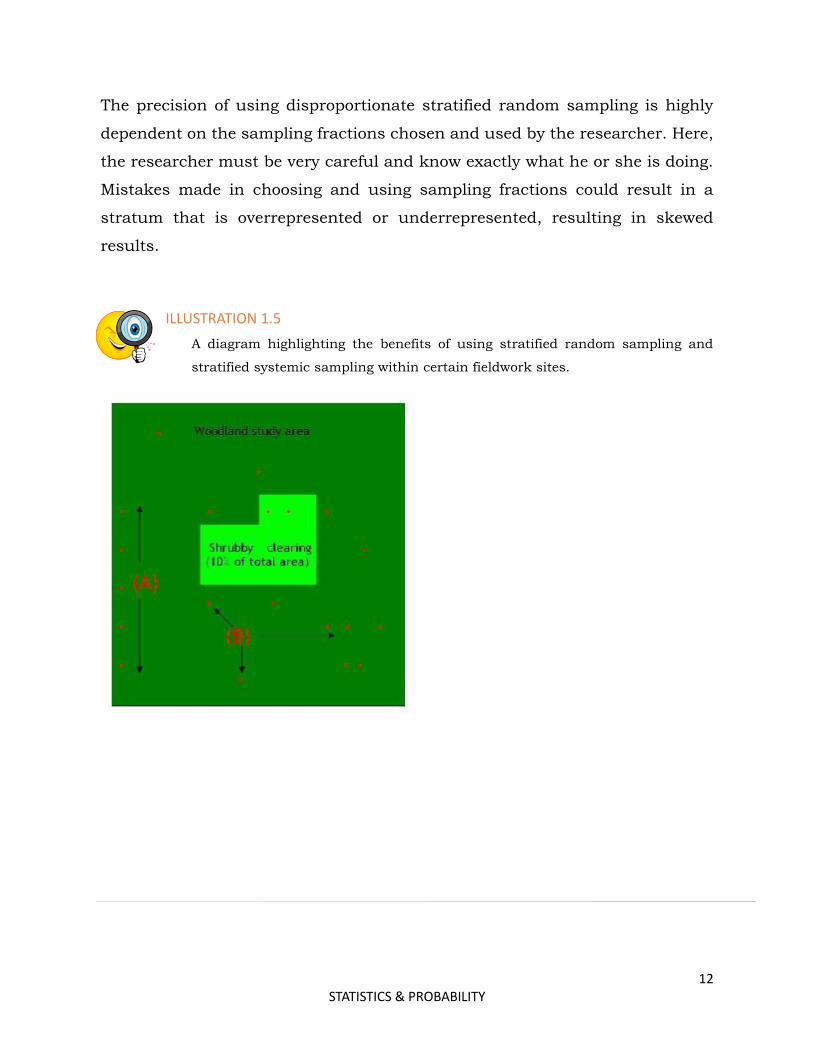
For example: if an area of woodland was the study site, there would likely be
different types of habitat (sub-sets) within it. Random sampling may altogether
‘miss' one or more of these.
Stratified sampling would take into account the proportional area of each
habitat type within the woodland and then each could be sampled accordingly;
if 20 samples were to be taken in the woodland as a whole, and it was found
that a shrubby clearing accounted for 10% of the total area, two samples would
need to be taken within the clearing. The sample points could still be identified
randomly (A) or systematically (B) within each separate area of woodland.
C. Proportionate Stratified Random Sampling
In proportional stratified random sampling, the size of each strata is
proportionate to the population size of the strata when looked at across the
entire population. This means that each stratum has the same sampling
fraction.
For example, let’s say you have four strata with population sizes of 200, 400,
600, and 800. If you choose a sampling fraction of ½, this means you must
randomly sample 100, 200, 300, and 400 subjects from each stratum
respectively. The same sampling fraction is used for each stratum regardless of
the differences in population size of the strata.
D. Disproportionate Stratified Random Sample
In disproportionate stratified random sampling, the different strata do not have
the same sampling fractions as each other. For instance, if your four strata
contain 200, 400, 600, and 800 people, you may choose to have different
sampling fractions for each stratum. Perhaps the first strata with 200 people
has a sampling fraction of ½, resulting in 100 people selected for the sample,
while the last strata with 800 people has a sampling fraction of ¼, resulting in
200 people selected for the sample.
12 STATISTICS & PROBABILITY
The precision of using disproportionate stratified random sampling is highly
dependent on the sampling fractions chosen and used by the researcher. Here,
the researcher must be very careful and know exactly what he or she is doing.
Mistakes made in choosing and using sampling fractions could result in a
stratum that is overrepresented or underrepresented, resulting in skewed
results.
ILLUSTRATION 1.5
A diagram highlighting the benefits of using stratified random sampling and
stratified systemic sampling within certain fieldwork sites.
13 STATISTICS & PROBABILITY
ADVANTAGES AND DISADVANTAGES OF STRATIFIED SAMPLING
Advantages:
It can be used with random or systematic sampling, and with point, line
or area techniques
If the proportions of the sub-sets are known, it can generate results which
are more representative of the whole population
It is very flexible and applicable to many geographical enquiries
Correlations and comparisons can be made between sub-sets
Disadvantages:
The proportions of the sub-sets must be known and accurate if it is to
work properly
It can be hard to stratify questionnaire data collection, accurate up to
date population data may not be available and it may be hard to identify
people's age or social background effectively
14 STATISTICS & PROBABILITY
NONPROBABILITY SAMPLING
The difference between nonprobability and probability sampling is that
nonprobability sampling does not involve random selection and probability
sampling does. Does that mean that nonprobability samples aren't
representative of the population? Not necessarily. But it does mean that
nonprobability samples cannot depend upon the rationale of probability theory.
At least with a probabilistic sample, we know the odds or probability that we
have represented the population well. We are able to estimate confidence
intervals for the statistic.
With nonprobability samples, we may or may not represent the population well,
and it will often be hard for us to know how well we've done so. In general,
researchers prefer probabilistic or random sampling methods over non-
probabilistic ones, and consider them to be more accurate and rigorous.
However, in applied social research there may be circumstances where it is not
feasible, practical or theoretically sensible to do random sampling. Here, we
consider a wide range of non-probabilistic alternatives.
ACCIDENTAL, HAPHAZARD OR CONVENIENCE SAMPLING
One of the most common methods of sampling goes under the various titles
listed here. I would include in this category the traditional "man on the street"
(of course, now it's probably the "person on the street") interviews conducted
frequently by television news programs to get a quick (although non
representative) reading of public opinion.
15 STATISTICS & PROBABILITY
In many research contexts, researchers sample simply by asking for volunteers.
Clearly, the problem with all of these types of samples is that there is no evidence
that they are representatives of the population the researchers interested in
generalizing to, and in many cases would clearly suspect that they are not.
PURPOSIVE SAMPLING
In purposive sampling, we sample with a purpose in mind. We
usually would have one or more specific predefined groups we are seeking. For
instance, have you ever run into people in a mall or on the street who are
carrying a clipboard and who are stopping various people and asking if they
could interview them? Most likely they are conducting a purposive sample (and
most likely they are engaged in market research). They might be looking for
Caucasian females between 30-40 years old. They size up the people passing
by and anyone who looks to be in that category they stop to ask if they will
participate. One of the first things they're likely to do is verify that the
respondent does in fact meet the criteria for being in the sample. Purposive
sampling can be very useful for situations where you need to reach a targeted
sample quickly and where sampling for proportionality is not the primary
concern. With a purposive sample, you are likely to get the opinions of your
target population, but you are also likely to overweight subgroups in your
population that are more readily accessible.
16 STATISTICS & PROBABILITY
HOW MUCH HAVE YOU LEARNED?
True or False
1. In reality there is enough time and resources that we don’t need to
adopt an efficient sampling technique
2. In probability sampling techniques there is a zero chance of being
selected.
3. A non-probability sampling technique represents a population
perfectly
4. There is no subjectivity in a random sampling
5. Stratified sampling ensures that results are proportional and
representative of the whole.
Answer here
1.
2.
3.
4.
5.
17 STATISTICS & PROBABILITY
PART 2: THE NORMAL DISTRIBUTION
Data can be "distributed" (spread out) in different ways. It can
be spread out more on the left ... or more on the right or it can
be all jumbled up but there are many cases where the data tends to be around
a central value with no bias left or right and that’s where normal distribution
comes in.
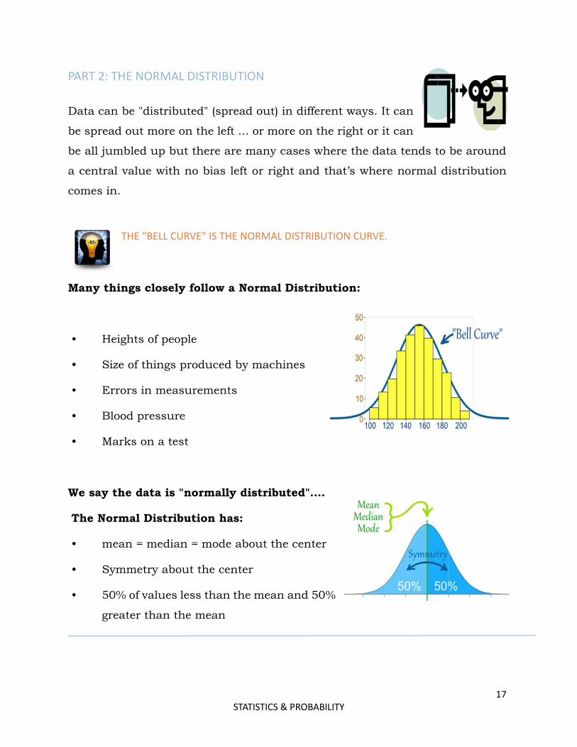
THE "BELL CURVE" IS THE NORMAL DISTRIBUTION CURVE.
Many things closely follow a Normal Distribution:
• Heights of people
• Size of things produced by machines
• Errors in measurements
• Blood pressure
• Marks on a test
We say the data is "normally distributed"….
The Normal Distribution has:
• mean = median = mode about the center
• Symmetry about the center
• 50% of values less than the mean and 50%
greater than the mean
18 STATISTICS & PROBABILITY
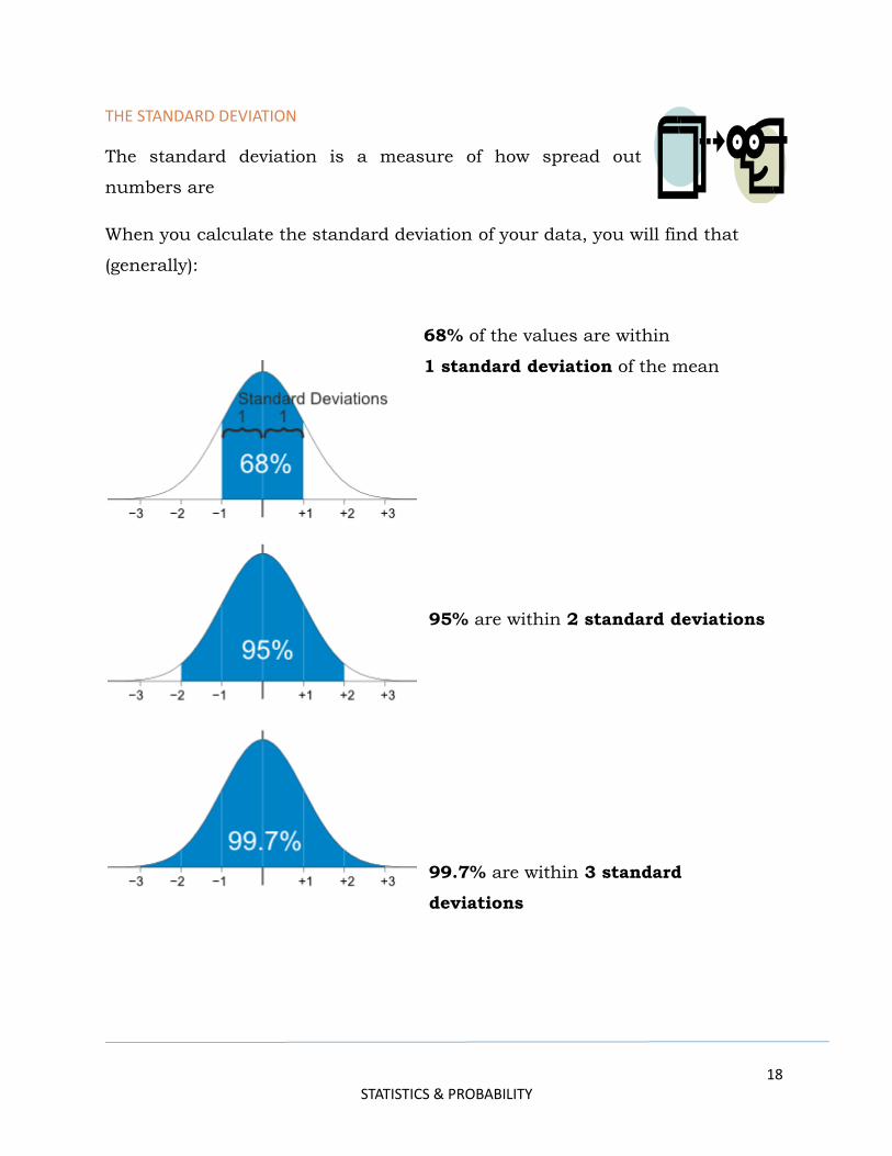
THE STANDARD DEVIATION
The standard deviation is a measure of how spread out
numbers are
When you calculate the standard deviation of your data, you will find that
(generally):
68% of the values are within
1 standard deviation of the mean
95% are within 2 standard deviations
99.7% are within 3 standard
deviations
19 STATISTICS & PROBABILITY
STANDARD SCORES
The number of standard deviations from the mean is also
called the "Standard Score", "sigma", "z-score", or “the z-value”
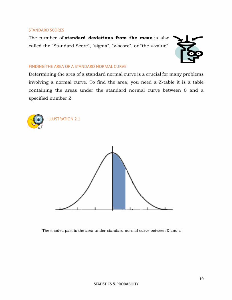
FINDING THE AREA OF A STANDARD NORMAL CURVE
Determining the area of a standard normal curve is a crucial for many problems
involving a normal curve. To find the area, you need a Z-table it is a table
containing the areas under the standard normal curve between 0 and a
specified number Z
ILLUSTRATION 2.1
The shaded part is the area under standard normal curve between 0 and z
20 STATISTICS & PROBABILITY
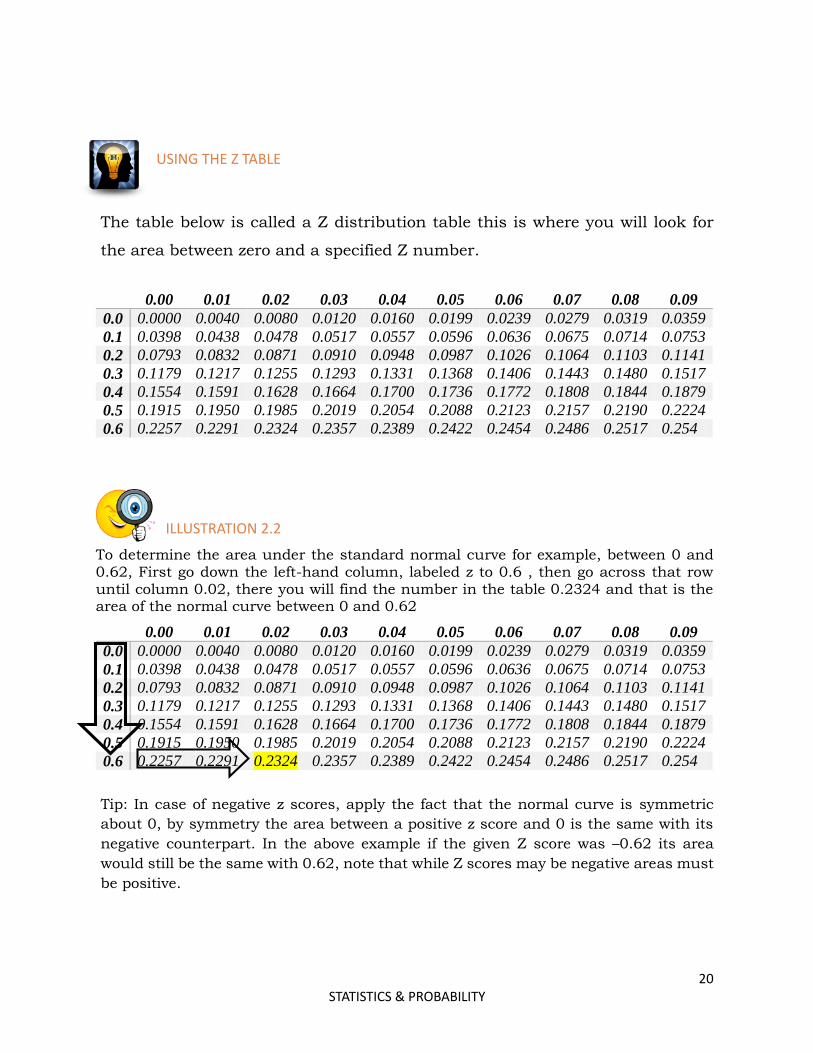
USING THE Z TABLE
The table below is called a Z distribution table this is where you will look for
the area between zero and a specified Z number.
ILLUSTRATION 2.2
To determine the area under the standard normal curve for example, between 0 and 0.62, First go down the left-hand column, labeled z to 0.6 , then go across that row until column 0.02, there you will find the number in the table 0.2324 and that is the area of the normal curve between 0 and 0.62
0.00 0.01 0.02 0.03 0.04 0.05 0.06 0.07 0.08 0.09
0.0 0.0000 0.0040 0.0080 0.0120 0.0160 0.0199 0.0239 0.0279 0.0319 0.0359
0.1 0.0398 0.0438 0.0478 0.0517 0.0557 0.0596 0.0636 0.0675 0.0714 0.0753
0.2 0.0793 0.0832 0.0871 0.0910 0.0948 0.0987 0.1026 0.1064 0.1103 0.1141
0.3 0.1179 0.1217 0.1255 0.1293 0.1331 0.1368 0.1406 0.1443 0.1480 0.1517
0.4 0.1554 0.1591 0.1628 0.1664 0.1700 0.1736 0.1772 0.1808 0.1844 0.1879
0.5 0.1915 0.1950 0.1985 0.2019 0.2054 0.2088 0.2123 0.2157 0.2190 0.2224
0.6 0.2257 0.2291 0.2324 0.2357 0.2389 0.2422 0.2454 0.2486 0.2517 0.254
Tip: In case of negative z scores, apply the fact that the normal curve is symmetric
about 0, by symmetry the area between a positive z score and 0 is the same with its
negative counterpart. In the above example if the given Z score was –0.62 its area
would still be the same with 0.62, note that while Z scores may be negative areas must
be positive.
0.00 0.01 0.02 0.03 0.04 0.05 0.06 0.07 0.08 0.09
0.0 0.0000 0.0040 0.0080 0.0120 0.0160 0.0199 0.0239 0.0279 0.0319 0.0359
0.1 0.0398 0.0438 0.0478 0.0517 0.0557 0.0596 0.0636 0.0675 0.0714 0.0753
0.2 0.0793 0.0832 0.0871 0.0910 0.0948 0.0987 0.1026 0.1064 0.1103 0.1141
0.3 0.1179 0.1217 0.1255 0.1293 0.1331 0.1368 0.1406 0.1443 0.1480 0.1517
0.4 0.1554 0.1591 0.1628 0.1664 0.1700 0.1736 0.1772 0.1808 0.1844 0.1879
0.5 0.1915 0.1950 0.1985 0.2019 0.2054 0.2088 0.2123 0.2157 0.2190 0.2224
0.6 0.2257 0.2291 0.2324 0.2357 0.2389 0.2422 0.2454 0.2486 0.2517 0.254
21 STATISTICS & PROBABILITY
MORE ON FINDING THE AREA….
To find the area of a normal curve to the right of a positive value
simply remember that a standard normal curve is symmetric about 0
it follows that the area under the normal curve to the right of z = 0 is 0.5
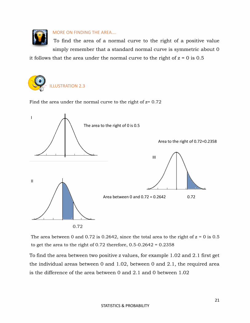
ILLUSTRATION 2.3
Find the area under the normal curve to the right of z= 0.72
I
The area to the right of 0 is 0.5
Area to the right of 0.72=0.2358
III
II
Area between 0 and 0.72 = 0.2642 0.72
0.72
The area between 0 and 0.72 is 0.2642, since the total area to the right of z = 0 is 0.5
to get the area to the right of 0.72 therefore, 0.5-0.2642 = 0.2358
To find the area between two positive z values, for example 1.02 and 2.1 first get
the individual areas between 0 and 1.02, between 0 and 2.1, the required area
is the difference of the area between 0 and 2.1 and 0 between 1.02
22 STATISTICS & PROBABILITY
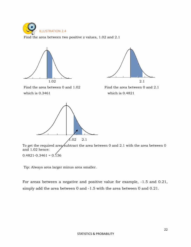
ILLUSTRATION 2.4
Find the area between two positive z values, 1.02 and 2.1
1.02 2.1
Find the area between 0 and 1.02 Find the area between 0 and 2.1
which is 0.3461 which is 0.4821
1.02 2.1
To get the required area subtract the area between 0 and 2.1 with the area between 0 and 1.02 hence:
0.4821-0.3461 = 0.136
Tip: Always area larger minus area smaller.
For areas between a negative and positive value for example, -1.5 and 0.21,
simply add the area between 0 and -1.5 with the area between 0 and 0.21.
23 STATISTICS & PROBABILITY
HOW MUCH HAVE YOU LEARNED?
I. True or False
1. In a normal curve the data distribution is concentrated on the right or left.
2. In a normal curve the mean, median and mode are not equal.
3. A normal distribution curve symmetrical about the mean.
4. The standard deviation is the measure how the numbers are close to the
mean.
5. You need a Chi-square table to find the area in a normal distribution curve.
6. To get the required area between two positive z values always add the area
larger to the area smaller.
Answer Here:
1.
2.
3.
4.
5.
6.
24 STATISTICS & PROBABILITY
PRACTICE WHAT YOU LEARNED
Find the area of the ff.
1. Between 0 and 1.98
2. Between 0 and 2.4
3. Between 0 and 2.1
4. Between 0 and 0.21
5. Between 0 and 0.67
6. Between 0 and 1.32
7. Between 0 and 2.32
8. Between 0 and 0.62
9. Between 0 and 2.97
10. Between 0 and 3.0
11. Between 0 and -1
12. Between 0 and -2
13. Between 0 and -2.4
14. Between 0 and -0.32
15. Between 0 and -1.67
16. Between 0 and – 1.2
17. Between 0 and – 1.64
18. Between 0 and -2.43
19. Between 0 and -3
20. Between 0 and -1.92
21. To the right of 2.5
22. To the right of 1.92
23. To the left of -1.42
24. To the left of -2.0
25. Between 1.0 and 2.2
26. Between 0.99 and 2
27. Between 1.21 and 2.8
28. Between -0.92 and 0. 91
29. Between -1 and 1
30. Between -2 and 2.6
25 STATISTICS & PROBABILITY
FINDING THE Z VALUE
Now we are done with finding the area in a normal curve using
z values but what if we are given the reverse? We are to find
the z value using a given area?
To find the value of the unknown Z score using a given area between it and 0,
simply look it up in the Z distribution table the Z value that corresponds to it,
let us say you have a given area of 0.3212 when you look it up in the table you
can see that the value it corresponds to is 0.92, it’s very similar in finding the
area albeit the reverse way.
When you are given an area to the right or left of an unknown Z score, simply
subtract the area given to 0.5 since we follow the assumption that each half of
the curve has an area of 0.5, then find the resulting difference in the Z table.
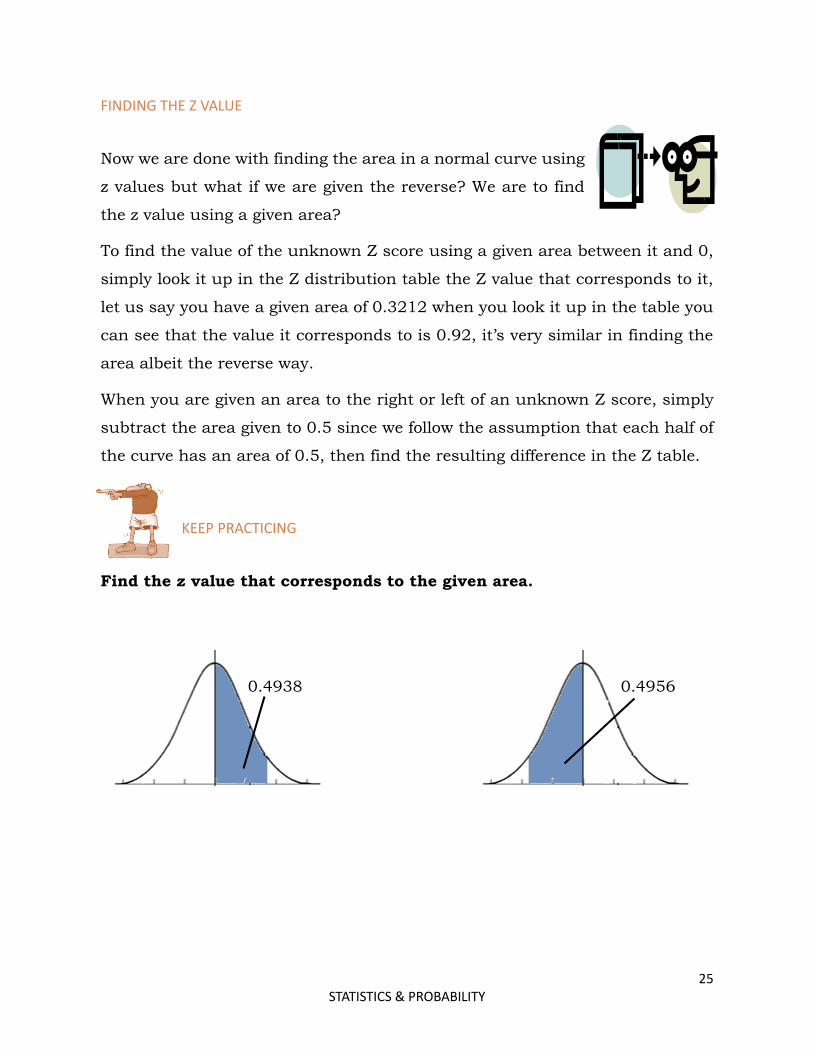
KEEP PRACTICING
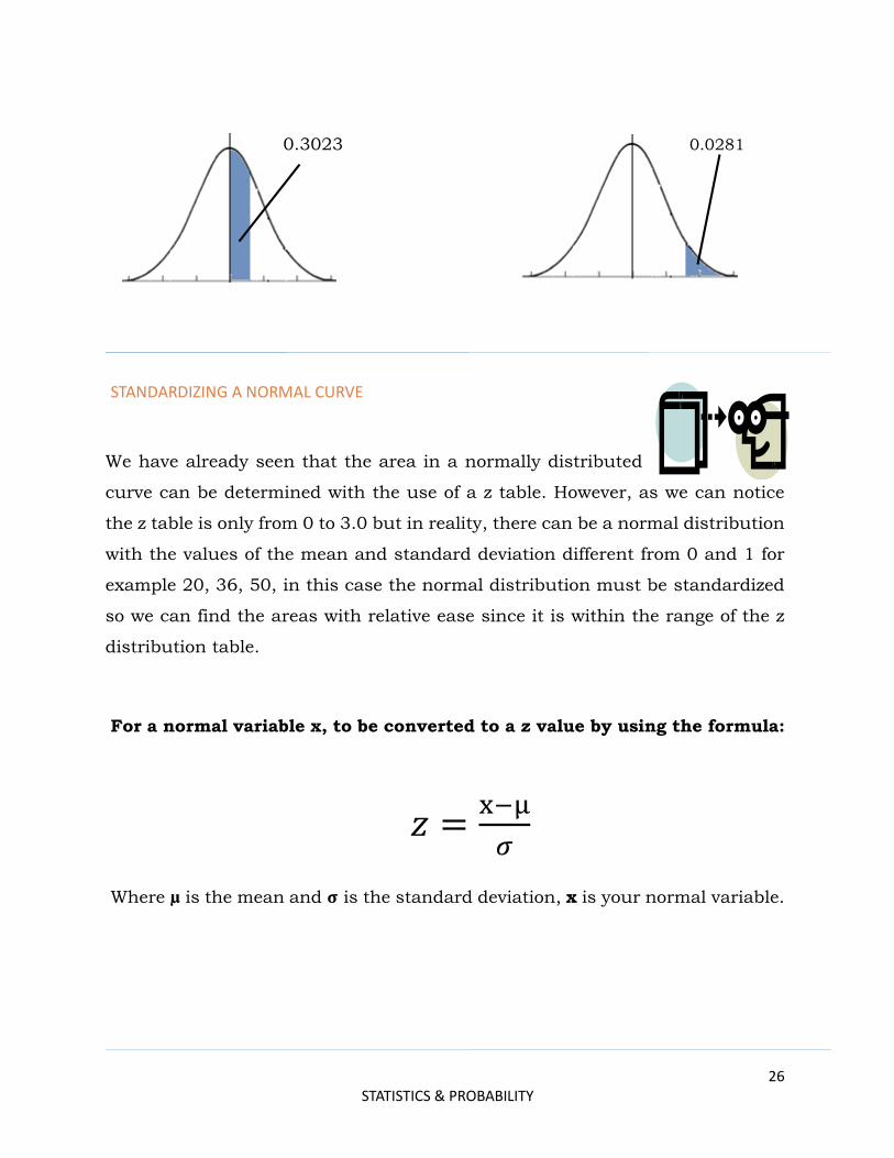
Find the z value that corresponds to the given area.
0.4938 0.4956
26 STATISTICS & PROBABILITY
0.3023 0.0281
STANDARDIZING A NORMAL CURVE
We have already seen that the area in a normally distributed
curve can be determined with the use of a z table. However, as we can notice
the z table is only from 0 to 3.0 but in reality, there can be a normal distribution
with the values of the mean and standard deviation different from 0 and 1 for
example 20, 36, 50, in this case the normal distribution must be standardized
so we can find the areas with relative ease since it is within the range of the z
distribution table.
For a normal variable x, to be converted to a z value by using the formula:
𝑧 =x−μ
𝜎
Where µ is the mean and 𝛔 is the standard deviation, x is your normal variable.
27 STATISTICS & PROBABILITY
ILLUSTRATION 2.5
Using the formula convert 20 to a z value with a mean of 25 and standard deviation of 2
𝑧 =x − μ
𝜎
Hence:
𝑧 =20 − 25
2
Z = -2.5
PRACTICE WHAT YOU LEARNED
Using the formula convert the following x values for a normal distribution to z values. Mean = 30; Standard deviation = 3
1. 26
2. 25
3. 19
4. 20
5. 31
6. 37
7. 32
8. 40
9. 26
10. 22
28 STATISTICS & PROBABILITY
To find the area between two x values for a normal distribution, convert first the
values of x to their corresponding z values, then find the area just like we did in
previous exercises.
KEEP PRACTICING
Find the area under the normal curve with parameters of mean 25 and
standard deviation of 2.25
1. Between 25 and 30
2. Between 25 and 20
3. Between 25 and 26
4. Between 25 and 28
5. Between 21and 26
6. Between 22 and 27
7. Between 23 and 20
8. Between 27 and 30
9. Between 28 and 21
10. Between 20 and 26
29 STATISTICS & PROBABILITY
ADDITIONAL THOUGHT….
Now we know how to standardize a normal curve by converting our x values to
z scores, but what about if we are given the reciprocal task? In that case we
need to simply use this formula.
𝑥 = z𝜎 + μ
THE NORMAL DISTRIBUTION CURVE AS PROBABILITY DISTRIBUTION CURVE
We have already learned how to find the area, z values and
standardization. Now we will move on to the application of the normal
distribution curve as a probability distribution curve for normally distributed
variables. Here the area under the curve corresponds to a probability or the
chance of being randomly chosen. Let us say we want to know the probability
of the values between 0 and 2 being chosen in a random draw, in this case the
area between 0 and 2 represents the probability of any values being chosen
between 0 and 2, and that would be 0.4772 or 47.72% probability.
For probabilities however, a special notation is used. For example if we are to
find the probability of any value between 0 and 2 we write it as P (0<z<2).
30 STATISTICS & PROBABILITY
PRACTICE WHAT YOU LEARNED
Write the following in probability notation
1. The probability between -2 and 0
2. The probability between 1 and 2.5
3. The probability between 2 and 3
4. The probability between -0.21 and 0
5. The probability between -1.89 and 1.5
6. The probability between 1.9 and 3
7. The probability between 2.75 and 1.9
8. The probability between 1.9 and 2.9
9. The probability between 0 and 2
10. The probability between 0 and 2.89
Now that we have familiarized ourselves with the probability
notation let us now move to solving probability problems by
finding the area, the process is just the same as the earlier
illustrations the only difference is that the area will not just an ordinary area
anymore, it represents probability and the givens are in probability notation.
31 STATISTICS & PROBABILITY
ILLUSTRATION 2.5
Find the probability using the standard normal distribution.
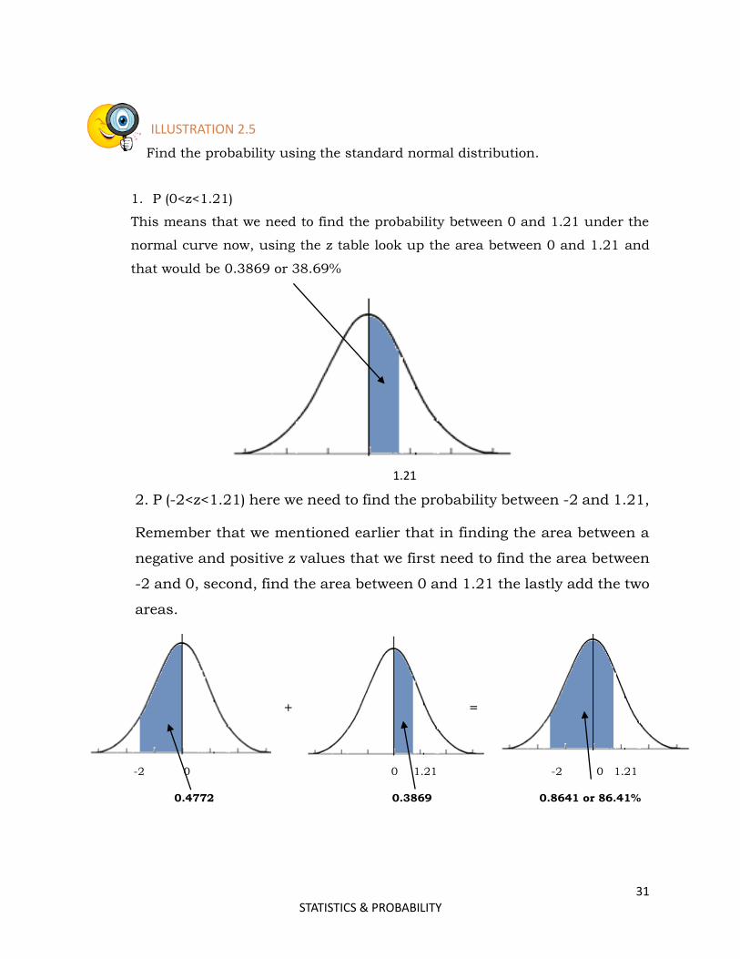
1. P (0<z<1.21)
This means that we need to find the probability between 0 and 1.21 under the
normal curve now, using the z table look up the area between 0 and 1.21 and
that would be 0.3869 or 38.69%
1.21
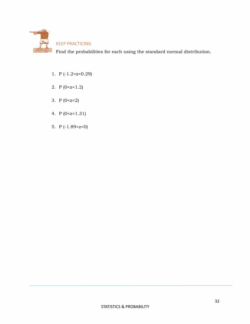
2. P (-2<z<1.21) here we need to find the probability between -2 and 1.21,
Remember that we mentioned earlier that in finding the area between a
negative and positive z values that we first need to find the area between
-2 and 0, second, find the area between 0 and 1.21 the lastly add the two
areas.
+ =
-2 0 0 1.21 -2 0 1.21
0.4772 0.3869 0.8641 or 86.41%
32 STATISTICS & PROBABILITY
KEEP PRACTICING
Find the probabilities for each using the standard normal distribution.
1. P (-1.2<z<0.29)
2. P (0<z<1.2)
3. P (0<z<2)
4. P (0<z<1.31)
5. P (-1.89<z<0)
33 STATISTICS & PROBABILITY
APPENDIX
REFERENCES/SOURCES:
MSA Statistics and Probability
Chapter 7 Normal Distribution Curve
Authors: Merlie S. Alferez and Ma. Cecilia Duro
Statistics and Probability Sampling Techniques http://www.rgs.org/OurWork/Schools/Fieldwork+and+local+learning/Fieldw
ork+techniques/Sampling+techniques.htm
Normal Distribution Curve
http://www.mathsisfun.com/data/standard-normal-distribution.html
http://www.google.com.ph/imgres?q=normal+distribution+curve&hl=fil&sa=X&biw=1280&bih=935&tbm=isch&tbnid=Uup00D7vCzMS5M:&imgrefurl=http:
//www.regentsprep.org/Regents/math/algtrig/ATS2/NormalLesson.htm&docid=H3dht9FFLdiDXM&imgurl=http://www.regentsprep.org/Regents/math/algtrig/ATS2/normal67.gif&w=679&h=357&ei=ip5FUcjsHYbqrAfa3YCoBA&zoo
m=1&ved=0CFUQhBwwAw&ved=1t:3588,r:3,s:0,i:85&iact=rc&dur=396&page=1&tbnh=163&tbnw=310&start=0&ndsp=18&tx=213&ty=102
34 STATISTICS & PROBABILITY
ANSWER KEY
How much have you learned? (Page 16)
1. False
2. False
3. False
4. True
5. True
How much have you learned? (Page 23)
1. False
2. False
3. True
4. True
5. False
6. False
35 STATISTICS & PROBABILITY
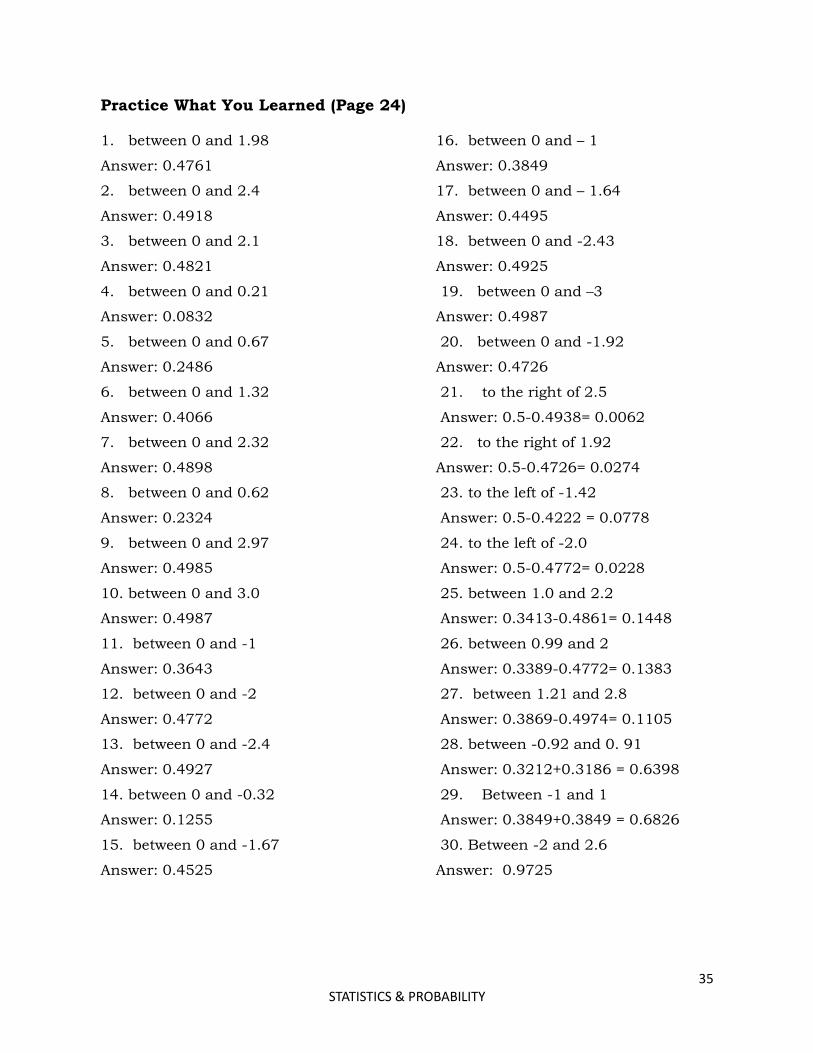
Practice What You Learned (Page 24)
1. between 0 and 1.98
Answer: 0.4761
2. between 0 and 2.4
Answer: 0.4918
3. between 0 and 2.1
Answer: 0.4821
4. between 0 and 0.21
Answer: 0.0832
5. between 0 and 0.67
Answer: 0.2486
6. between 0 and 1.32
Answer: 0.4066
7. between 0 and 2.32
Answer: 0.4898
8. between 0 and 0.62
Answer: 0.2324
9. between 0 and 2.97
Answer: 0.4985
10. between 0 and 3.0
Answer: 0.4987
11. between 0 and -1
Answer: 0.3643
12. between 0 and -2
Answer: 0.4772
13. between 0 and -2.4
Answer: 0.4927
14. between 0 and -0.32
Answer: 0.1255
15. between 0 and -1.67
Answer: 0.4525
16. between 0 and – 1
Answer: 0.3849
17. between 0 and – 1.64
Answer: 0.4495
18. between 0 and -2.43
Answer: 0.4925
19. between 0 and –3
Answer: 0.4987
20. between 0 and -1.92
Answer: 0.4726
21. to the right of 2.5
Answer: 0.5-0.4938= 0.0062
22. to the right of 1.92
Answer: 0.5-0.4726= 0.0274
23. to the left of -1.42
Answer: 0.5-0.4222 = 0.0778
24. to the left of -2.0
Answer: 0.5-0.4772= 0.0228
25. between 1.0 and 2.2
Answer: 0.3413-0.4861= 0.1448
26. between 0.99 and 2
Answer: 0.3389-0.4772= 0.1383
27. between 1.21 and 2.8
Answer: 0.3869-0.4974= 0.1105
28. between -0.92 and 0. 91
Answer: 0.3212+0.3186 = 0.6398
29. Between -1 and 1
Answer: 0.3849+0.3849 = 0.6826
30. Between -2 and 2.6
Answer: 0.9725
36 STATISTICS & PROBABILITY
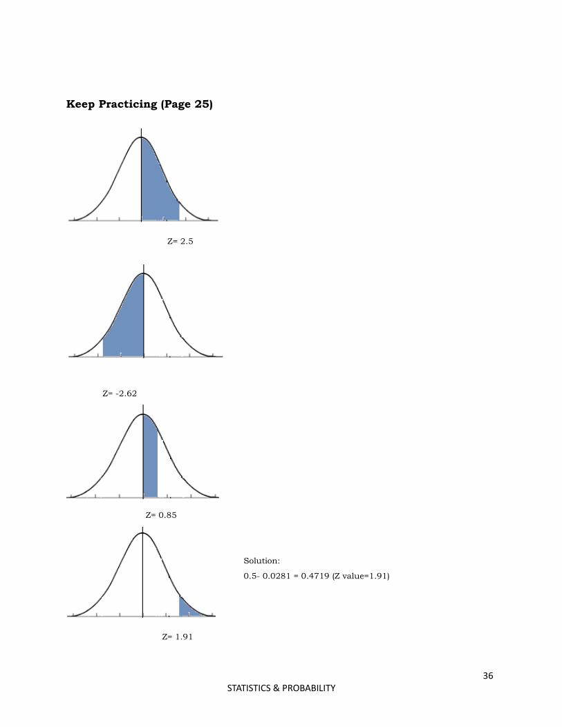
Keep Practicing (Page 25)
Z= 2.5
Z= -2.62
Z= 0.85
Solution:
0.5- 0.0281 = 0.4719 (Z value=1.91)
Z= 1.91
37 STATISTICS & PROBABILITY
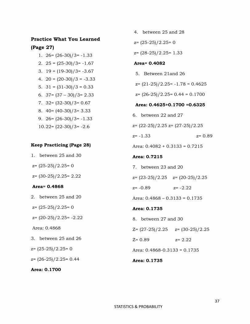
Practice What You Learned
(Page 27)
1. 26= (26-30)/3= -1.33
2. 25 = (25-30)/3= -1.67
3. 19 = (19-30)/3= -3.67
4. 20 = (20-30)/3 = -3.33
5. 31 = (31-30)/3 = 0.33
6. 37= (37 – 30)/3= 2.33
7. 32= (32-30)/3= 0.67
8. 40= (40-30)/3= 3.33
9. 26= (26-30)/3= -1.33
10. 22= (22-30)/3= -2.6
Keep Practicing (Page 28)
1. between 25 and 30
z= (25-25)/2.25= 0
z= (30-25)/2.25= 2.22
Area= 0.4868
2. between 25 and 20
z= (25-25)/2.25= 0
z= (20-25)/2.25= -2.22
Area: 0.4868
3. between 25 and 26
z= (25-25)/2.25= 0
z= (26-25)/2.25= 0.44
Area: 0.1700
4. between 25 and 28
z= (25-25)/2.25= 0
z= (28-25)/2.25= 1.33
Area= 0.4082
5. Between 21and 26
z= (21-25)/2.25= -1.78 = 0.4625
z= (26-25)/2.25= 0.44 = 0.1700
Area: 0.4625+0.1700 =0.6325
6. between 22 and 27
z= (22-25)/2.25 z= (27-25)/2.25
z= -1.33 z= 0.89
Area: 0.4082 + 0.3133 = 0.7215
Area: 0.7215
7. between 23 and 20
z= (23-25)/2.25 z= (20-25)/2.25
z= -0.89 z= -2.22
Area: 0.4868 – 0.3133 = 0.1735
Area: 0.1735
8. between 27 and 30
Z= (27-25)/2.25 z= (30-25)/2.25
Z= 0.89 z= 2.22
Area: 0.4868-0.3133 = 0.1735
Area: 0.1735
38 STATISTICS & PROBABILITY
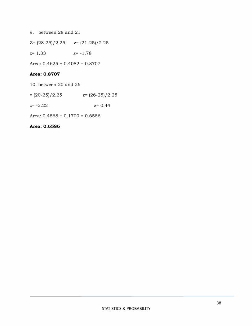
9. between 28 and 21
Z= (28-25)/2.25 z= (21-25)/2.25
z= 1.33 z= -1.78
Area: 0.4625 + 0.4082 = 0.8707
Area: 0.8707
10. between 20 and 26
= (20-25)/2.25 z= (26-25)/2.25
z= -2.22 z= 0.44
Area: 0.4868 + 0.1700 = 0.6586
Area: 0.6586
39 STATISTICS & PROBABILITY
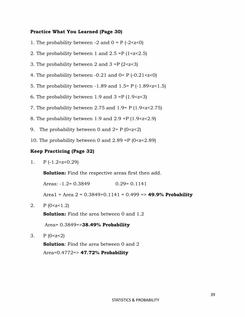
Practice What You Learned (Page 30)
1. The probability between -2 and 0 = P (-2<z<0)
2. The probability between 1 and 2.5 =P (1<z<2.5)
3. The probability between 2 and 3 =P (2<z<3)
4. The probability between -0.21 and 0= P (-0.21<z<0)
5. The probability between -1.89 and 1.5= P (-1.89<z<1.5)
6. The probability between 1.9 and 3 =P (1.9<z<3)
7. The probability between 2.75 and 1.9= P (1.9<z<2.75)
8. The probability between 1.9 and 2.9 =P (1.9<z<2.9)
9. The probability between 0 and 2= P (0<z<2)
10. The probability between 0 and 2.89 =P (0<z<2.89)
Keep Practicing (Page 32)
1. P (-1.2<z<0.29)
Solution: Find the respective areas first then add.
Areas: -1.2= 0.3849 0.29= 0.1141
Area1 + Area 2 = 0.3849+0.1141 = 0.499 => 49.9% Probability
2. P (0<z<1.2)
Solution: Find the area between 0 and 1.2
Area= 0.3849=>38.49% Probability
3. P (0<z<2)
Solution: Find the area between 0 and 2
Area=0.4772=> 47.72% Probability
40 STATISTICS & PROBABILITY
4. P (0<z<1.31)
Solution: Find the are between 0 and 1.31
Area= 0.4049=> 40.49% Probability
5. P (-1.89<z<0)
Solution: Find the area between 0 and -1.89
Area= 0.4706 =>47.06% Probability