STATISTICS AND RESEARCH

METHODS EXAM SYNOPSIS Bsc. in International Business and Politics

Copenhagen Business School 2016

Students and CPR numbers: Rasmus Grand Berthelsen (140993-1827)

Joakim Viggers (160594-1741) Mette Schrøder (240894-1302)

Mads Tryggedsson (130693-1551) Mie Dahl (140894-1810)

Group Number: 4 Hand-in date: 11th of January 2016

Number of pages: 14 STU-count: 32,928 (14.5 standard pages)

Page 1 of 14

Introduction This data set from the US veterans association concerns a group of donors who skipped one year of

donations. We focus on analyzing two variables as response variables: the average gift size from each subject

and a binary variable recording whether a donation was made or not. Thus, LogAvgGift and DidDonate are

response variables and the remaining variables are explanatory.

Question 1 Give a brief description of the distribution of selected variables in the data set. In particular, compare

the distribution of logAvgGift and its untransformed counterpart.

We start our investigation of the data by doing descriptive statistics. We have selected some variables that

we find relevant for our investigation. For quantitative variables, we want to see if there is anything

remarkable to note about their skewness and potential outliers, and for categorical variables we look at the

frequency of observations in each of the categories. From the investigated variables, DidDonate, MoreThanOneGift and AgeGroup are classified as categorical

variables. Age, AvgGift and LogAvgGift are classified as quantitative variables.

AvgGift The variable AvgGift is slightly skewed to the right with a

mean of 13.7 and a median of 12.3. The interquartile range

(IQR) is 7.11 (from 9 to 16.11). Thus, 50 % of the

observations lie between 9 and 16.11. The range of

observations is from 2.12 to 200, so the right tail is long.

According to the 1.5 x IQR criterion, we identify 341

possible outliers.

LogAvgGift The variable LogAvgGift, which is the log base 10 of

AvgGift, has an approximate normal distribution. A

histogram of the distribution shows that it is almost

perfectly bell-shaped with a median of 1.09 and a mean of

1.08.

Comparison of the distribution between AvgGift and LogAvgGift

We observe that LogAvgGift is closer to being normally distributed than

AvgGift. LogAvgGift has been converted into base 10 logarithm to

diminish the spread of the data and correct for potential outliers.

Age From the table (see appendix 1A) we see that the mean age of those who

have donated in the past is 51. The boxplot shows that donators are

usually middle-aged or old, as 75 % of previous donators are 43 years old or above.

DidDonate This is a binary categorical variable observing whether the respondent donated after receiving the mailing.

95.25 % of the respondents did not donate after receiving the mailing. Conversely, 4.75 % did donate (see

appendix 1B).

MoreThanOneGift This is a binary categorical variable showing whether the respondent has donated more than once prior to

Page 2 of 14

skipping one year of donations. 47.19 % of the respondents have not donated more than once, 52.81% have

(see appendix 1C).

Age Group This variable observes within which age group the respondent falls. It is an ordinal categorical variable. The

distribution of respondents in different age groups is: Age 20-29 2.67%, age 30-39 13.8%, age 40-49

27.39%, age 50-59 29% and age 60-69 27.14% (see appendix 1D).

Question 2 Compare the proportion of subjects who donated (as recorded in DidDonate) depending on the value

of MoreThanOneGift. Give a confidence interval for the difference in proportions and for the odds

ratio. Also, investigate the effect of age by analyzing a contingency table of AgeGroup and DidDonate.

In this question, we start doing inferential statistics.

The contingency table shows that 5.66 % of the subjects who previously

donated more than one gift did donate again, and that 3.94 % of the subjects

who did not previously donate more than one gift did donate again. To

compare whether there is a significant difference between the two sample

proportions, we conduct a two-sided significance test.

Z test for the difference in proportions

1. Assumptions We have a categorical variable for two groups and assume randomization. Also, we assume that n1

and n2 are sufficiently large so that 𝑛 ∗ 𝑝 > 5 and 𝑛(1 − 𝑝) > 5 which we see holds.

2. Hypotheses

Our null hypothesis is that there is no difference between 𝑝1 and 𝑝2: 𝐻0: 𝑝1 = 𝑝2

Our alternative hypothesis is that 𝑝1 is different from 𝑝2: 𝐻𝑎: 𝑝1 ≠ 𝑝2

3. Test statistic

𝑧 =(𝑝1−𝑝2)−0

𝑠𝑒0 with 𝑠𝑒0 = √�̂�(1 − �̂�) (

1

𝑛1+

1

𝑛2), where �̂� is the pooled estimate

The pooled estimate is calculated: �̂� =248+193

9277= 0.047537

𝑧 =(0.0566−0.0394)−0

√0.047537 (1−0.047537)(1

4378+

1

4899)

=0.0172

0.004425= 3.887

4. P-value

The P-value for a two-sided alternative hypothesis is the two-tail probability from a standard normal

distribution resulting in the same value of the observed test statistic, i.e. z-value, or more extreme

values assuming H0 is true. A z-score of 3.887 is far out in the right tail. For a large sample test, the

critical z-value is ±1.96, so the z-score already indicates that H0 might not hold. For a z-score of

3.887 the corresponding P-value is < 0.0001

5. Conclusion A P-value less than 0.0001 is below our significance level of 0.05. Therefore, we conclude that there

is statistical evidence to reject the null hypothesis. Hence, the proportion of people who donated is

statistically different based on whether they previously donated more than one gift or not.

Page 3 of 14

Confidence Interval for the difference in proportions

We construct a confidence interval (CI) for the difference between the two population proportions. The CI

gives us a range of possible values for the parameter. It can be calculated: the point estimate ± 1.96 × the

standard error. We use 1.96 because this is the critical value for a 95 % confidence interval when conducting

a z test.

The formula for a 95 % CI for two proportions is �̂�1 − �̂�2 ± 𝑧𝑎/2 ∗ 𝑠𝑒 where 𝑠𝑒 = √𝑝1(1−𝑝1)

𝑛1+

𝑝2(1−�̂�2)

𝑛2

𝐶𝐼 = (0.0566 − 0.0394) ± 1.96 ∗ √0.0566(1−0.0566)

4378+

0.0394(1−0.0394)

4899= [0.00845; 0.02595]

The confidence interval shows that the difference in the proportion of people who donated depending on

whether they previously donated more than one gift with 95 % confidence lies between 0.00845 and 0.02595.

Therefore, we can be 95 % confident that the population proportion of people who did donate is between 0.8

% and 2.6 % higher for subjects who previously donated more than one gift than for subjects who did not.

Confidence Interval for the odds ratio

The odds ratio describes the odds of an event occurring in one group relative to the odds of it occurring in

another group. We construct a CI for the odds ratio.

We calculate the odds ratio, which can be estimated from the observed counts:

𝑂𝑅 =𝑛1,1/𝑛1,2

𝑛2,1/𝑛2,2=

248/4130

193/4706= 1.464186

We take the log of odds ratio: log(𝑂𝑅) = log (1.464186) = 0.3813

We calculate the standard error:

𝑠𝑒 = √1

𝑛1,1+

1

𝑛1,2+

1

𝑛2,1+

1

𝑛2,2= √

1

248+

1

4706+

1

193+

1

4130= 0.09833

We add and subtract 1.96 multiplied by the standard error to/from the log of odds ratio to find a CI

on the log scale. We use 1.96, as this is the critical value when constructing a 95 % CI for a normal

distribution.

𝐶𝐼(log(𝑂𝑅)) = log(𝑂𝑅) ± 1.96 ∗ 𝑠𝑒 = 0.3813 ± 1.96 ∗ 0.09833 = [0.1886; 0.574]

We take antilogarithms of both ends to find to the interval for the odds ratio itself.

𝐶𝐼(𝑂𝑅) = [𝑒0.1886 ; 𝑒0.574] = [1.208; 1.775]

We see that the CI for the odds ratio does not contain 1, and we are 95 % confident that the odds ratio is

between 1.208 and 1.775. With 95 % confidence, we conclude that there is a difference between the odds of

donating for people who previously donated more than one gift and for people who did not. An odds ratio of

1 would mean that the odds of the two groups were equal.

Investigation of the effect of age on donation

We perform a chi-squared test of independence to investigate whether age has

an effect on donation. The chi-squared statistic summarizes how far each

observed cell count falls from the predicted value assuming that H0 is true.

1. Assumptions We have two categorical variables, AgeGroup and DidDonate, and

we assume randomization. We assume that the expected cell count

will be larger than or equal to 5 in all cells.

2. Hypotheses Our null hypothesis is that age does not have an effect on donation:

H0: The two variables are independent.

Page 4 of 14

Our alternative hypothesis is that there is an association between age and donation: Ha: The two

variables are dependent

3. Test statistic

𝜒2 = ∑(𝑜𝑏𝑠𝑒𝑟𝑣𝑒𝑑 𝑐𝑜𝑢𝑛𝑡−𝑒𝑥𝑝𝑒𝑐𝑡𝑒𝑑 𝑐𝑜𝑢𝑛𝑡)2

𝑒𝑥𝑝𝑒𝑐𝑡𝑒𝑑 𝑐𝑜𝑢𝑛𝑡=

(11−11.79)2

11.79+

(52−60.85)2

60.85… +

(2390−2398.3)2

2398.3= 5.54

In which the expected count is 𝑟𝑜𝑤 𝑡𝑜𝑡𝑎𝑙∗𝑐𝑜𝑙𝑢𝑚𝑛 𝑡𝑜𝑡𝑎𝑙

𝑡𝑜𝑡𝑎𝑙 𝑐𝑜𝑢𝑛𝑡

4. P-value

The P-value for a chi-squared test is the right-tail probability for a chi-squared distribution with

𝑑𝑓 = (𝑟 − 1) ∗ (𝑐 − 1), resulting in the same or a more extreme value than the observed chi-squared

test statistic, assuming H0 is true.

The chi-squared test statistic is 5.54. For this test statistic, with a chi-squared distribution given 𝑑𝑓 =(2 − 1) ∗ (5 − 1) = 4, the p-value is 𝑃 = 0.236

5. Conclusion A P-value of 0.236 is higher than our significance level of 0.05, so we conclude that there is not

statistical evidence to reject the null hypothesis of no dependence between the two variables

DidDonate and AgeGroup. Thus, we cannot reject that there is no dependence between age group

and whether people did donate.

Question 3 Compare logAvgGift between respondents who have HomePhone equal to 1 and 0. Include a statistical

test and give a 95% confidence interval for the difference between the population means. Also,

compare logAvgGift between the different values of AgeGroup

T-test for the difference in logAvgGift depending on HomePhone

1. Assumptions

We have a quantitative variable for two groups and assume randomization. We also assume

normal population distribution for each group. Lastly, we assume equal variance based on a

Levene test in JMP giving a p-value of 0.4188 (see appendix 3A).

2. Hypotheses

Our null hypothesis is that there is no difference between 𝜇1 and 𝜇2: 𝐻0: 𝜇1 = 𝜇2

Our alternative hypothesis is that 𝜇1 is different from 𝜇2: 𝐻𝑎: 𝜇1

≠ 𝜇2

3. Test Statistic

From JMP we get the output (see appendix 3B):

For HomePhone = 1: 𝑥1̅̅ ̅ = 1.07342, 𝑠1 = 0.205353 and 𝑛1 = 4880

For HomePhone = 0: 𝑥2̅̅ ̅ = 1.09710 𝑠2 = 0.209808 and 𝑛2 = 4397

𝑡 =(𝑥1̅̅ ̅̅ ̅−𝑥2)̅̅ ̅̅ ̅−0

𝑠𝑒, where 𝑠𝑒 = √

(𝑛1−1)𝑆12+(𝑛2−1)𝑆2

2

𝑛1+𝑛2−2∗ √

1

𝑛1+

1

𝑛2

𝑡 =(1.07342−1.09710)−0

√(4880−1)0.2053532+(4397−1)0.2098082

4880+4397−2∗√

1

4880+

1

4397

= −5.489

4. P-Value

Page 5 of 14

The P-value is the two-tail probability of obtaining the same value of the t-test statistic or more

extreme values in a t-distribution with 𝑑𝑓 = 𝑛 − 2, assuming the null hypothesis is true.

A t-score of -5.489 is far out in the left tail. For a large sample test, the critical value is ±1.96, so the

t-score already indicates that the null hypothesis might not hold true.

The t-test statistic is -5.489. For this test statistic, with a t-distribution given 𝑑𝑓 = 9277 − 2 =9275, the p-value is 𝑃 < 0.0001.

5. Conclusion

A P-value less than 0.0001 is below our significance level of 0.05. We conclude that there is

statistical evidence to reject the null hypothesis. Hence, the means of LogAvgGift is statistically

different based on whether they have a home phone or not.

Confidence interval for the difference between the population means

We construct a CI for the difference between the two population means. We use 1.96 when calculating it,

because this is the critical value in a t-distribution for a 95 % confidence interval when 𝑑𝑓 > 100.

𝐶𝐼: (𝑥1̅̅ ̅ − 𝑥2̅̅ ̅) ± 𝑡.025 ∗ (𝑠𝑒), in which the standard error is

𝑠𝑒 = √(𝑛1−1)𝑆1

2+(𝑛2−1)𝑆22

𝑛1+𝑛2−2∗ √

1

𝑛1+

1

𝑛2= √

(4880−1)0.2053532+(4397−1)0.2098082

4880+4397−2∗ √

1

4880+

1

4397= 0.004314

𝐶𝐼: (1.07342 − 1.09710) ± 1.96 · 0.004314 = [−0.01522; −0.03214]

The CI does not contain 0 (corresponding with our rejection of H0 in the previous section) and with 95 %

confidence the true population difference in means of LogAvgGift between people with and without a home

phone will be between -0.01522 and -0.03214.

F-test for comparison of LogAvgGift between the different values of AgeGroup

We look at AgeGroup as the explanatory variable for LogAvgGift. We compare the means of the different

age groups and conduct an analysis of variance (ANOVA), which compares means of several groups. The

purpose is to determine whether there is dependency between LogAvgGift and AgeGroup.

1. Assumptions

We have a quantitative variable for more than two groups, and assume normal distributions of the

response variables. We also assume the same standard deviation for each group, and lastly we

assume randomization.

2. Hypothesis

Our null hypothesis is that there is no difference in the size of LogAvgGift across the different age

groups: 𝐻0: 𝜇1 = 𝜇2 … = 𝜇𝑔

Our alternative hypothesis is that at least two of the population means are unequal.

3. Test statistic

The sample distributions has degrees of freedom:

𝑑𝑓1 = 𝑔 − 1 = 5 − 1 = 4

𝑑𝑓2 = 𝑁 − 𝑔 = 9277 − 5 = 9272

𝐹 =𝑉𝑎𝑟𝑖𝑎𝑏𝑖𝑙𝑖𝑡𝑦𝐵𝑒𝑡𝑤𝑒𝑒𝑛𝐺𝑟𝑜𝑢𝑝𝑠

𝑉𝑎𝑟𝑖𝑎𝑏𝑖𝑙𝑖𝑡𝑦𝑊𝑖𝑡ℎ𝑖𝑛𝐺𝑟𝑜𝑢𝑝𝑠=

𝑆𝑆𝐴𝑔𝑒𝐺𝑟𝑜𝑢𝑝/𝑑𝑓1

𝑆𝑆𝑒𝑟𝑟𝑜𝑟/𝑑𝑓2=

2.04824/4

398.503/9272= 11.9141

4. P-Value

The P-value is the right-tail probability of obtaining the same value of the F-test statistic or more

Page 6 of 14

extreme values in an F-distribution with 𝑑𝑓1 = 4 and 𝑑𝑓2 = 9272 assuming H0 is true. We find an F-

test = 11.9141, and the larger the f-test, the stronger the evidence against H0.

For this test statistic, with an F-distribution given 𝑑𝑓1 = 4 and 𝑑𝑓2 = 9272, the P-value is 𝑃 <0.0001.

5. Conclusion

A P-value less than 0.0001 is below our significance level of 0.05. We conclude that there is

statistical evidence to reject the null hypothesis that the means of LogAvgGift are equal for all age

groups. Hence, at least two of the means of LogAvgGift are unequal, indicating that LogAvgGift

might depend on age group.

Question 4 Fit a simple linear regression model in which logAvgGift is described by Age. Does a quadratic model

or maybe even a higher order polynomial fit the data better? Discuss your findings in relation to the

analysis in the previous question where AgeGroup was used as the descriptive variable. Discuss

whether the model assumptions are satisfied reasonably well.

Fit linear regression

In this question we have two quantitative variables. A linear regression has the

formula 𝑌 = 𝛽0 + 𝛽1 ∗ 𝑥 + 𝜖. Using JMP we construct a scatterplot (see

appendix 4A) and fit a linear regression using the method of ordinary least

squares, where age is the explanatory variable and logAvgGift is the response

variable. We get:

𝐿𝑜𝑔𝐴𝑣𝑔𝐺𝑖𝑓𝑡 = 1.14066 − 0.001096 ∗ 𝐴𝑔𝑒

The negative slope of -0.001096 indicates that logAvgGift decreases with age. The P-value is less than

0.0001, which is below our 0.05 significance level. This indicates that the coefficient Age is statistically

significant in explaining ‘logAvgGift’.

Quadratic polynomial model

Transforming the above simple linear regression model into a quadratic model, we get:

𝐿𝑜𝑔𝐴𝑣𝑔𝐺𝑖𝑓𝑡 = 0.97087 + 0.00607 ∗ 𝐴𝑔𝑒 − 0.00007 ∗ 𝐴𝑔𝑒2

Both coefficients, Age and Age2, are statistically significant in explaining

logAvgGift. Therefore, we suggest using the quadratic polynomial model, since

this contains more statistically significant coefficients. We continue to

investigate whether a model of higher polynomial order fits the data better.

Cubic polynomial model

Transforming the above model into a cubic model, we get:

𝐿𝑜𝑔𝐴𝑣𝑔𝐺𝑖𝑓𝑡 = 1.0906 − 0.00196 ∗ 𝐴𝑔𝑒 + 0.0001 ∗ 𝐴𝑔𝑒2 − 0.000001 ∗

𝑎𝑔𝑒3

Now none of the coefficients are statistically significant in explaining

logAvgGift. Therefore, we do not suggest using this model, but the previous

quadratic model instead.

Page 7 of 14

Supporting our conclusion, we present the R2 adjusted values. These values

show the R2 including a degrees of freedom-adjustment, which penalizes the

for adding insignificant parameters. The quadratic model gives the highest R2

adjusted value, which corresponds with our suggestion of this model.

Discussion of findings in relation to analysis of previous question

In the previous ANOVA test, we found that the means are not equal across age groups. Thus, it is no surprise

that age is significant on the size of logAvgGift. The predicted logAvgGift starts by increasing by 0.00607

with age but it decreases by 0.00007 again at older ages.

Model Assumptions:

1. The regression model is linear in coefficients, correctly specified and has an additive error term.

2. The expected values of all residuals (i.e. the mean) must equal zero

3. All explanatory variables are uncorrelated with the residuals

4. No serial correlation of errors i.e. no system of errors

5. Equal variation for all values of �̂�

6. Errors are normally distributed

Assumption 1

𝐿𝑜𝑔𝐴𝑣𝑔𝐺𝑖𝑓𝑡 = 1.14066 − 0.001096 ∗ 𝑎𝑔𝑒

It can be seen from the formula that there is linearity in coefficients

Assumption 2

As it can be seen from the graph “Residual logAvgGift vs. Predicted

logAvGift” the mean of the residuals approximately centres around

zero.

Assumption 3

As it can can be seen from “Residual logAvgGift vs. Age” there is no

clear pattern i.e. the explanatory variable seem to have no effect on the

residuals.

Assumption 4

As it can be seen from “Residual logAvgGift vs. Predicted logAvGift”

there is no clear pattern of errors.

Assumption 5

As it can be seen from “Residual logAvgGift vs. Predicted logAvGift”

the variations for the values of logAvgGift are approximately equal,

though the variance might be slightly smaller at younger ages. However,

we do not consider this significant.

Assumption 6

As it can be seen from the graph “Residual logAvgGift”, some residuals

fall outside our 95% CI (indicated by the dotted red lines), although they

do approximately form a straight line, indicating a normal distribution.

It can be argued that the assumption is violated, which might complicate

the predictive power of the model.

R2 Adjusted

Simple 0.00331429

Quadratic 0.00525301

Cubic 0.00522156

Page 8 of 14

Question 5 Extend the regression model to a multiple linear regression model by further including logPerCapInc,

logMedHouseHoldInc, HomePhone, PcOwner, Cars and School. Retain a quadratic polynomial in Age

(this can be done using Macro/Polynomial to Degree in the Fit

Model form).

Since we now have several independent variables, we extend our

simple regression to a multiple regression. We model the expected

value of LogAvgGift conditional on LogPerCapInc,

LogMedHouseHoldInc, HomePhone, PcOwner, Cars, School, Age

and Age2.

Our new model is:

𝑙𝑜𝑔𝐴𝑣𝑔𝐺𝑖𝑓𝑡 = 0.53678 + 0.00543𝐴𝑔𝑒 − 0.00006𝐴𝑔𝑒2 + 0.00733𝑆𝑐ℎ𝑜𝑜𝑙 − 0.03078𝐶𝑎𝑟𝑠 +0.02441𝐻𝑜𝑚𝑒𝑃ℎ𝑜𝑛𝑒[0] − 0.01443𝑃𝐶𝑂𝑤𝑛𝑒𝑟[0] + 0.03937𝑙𝑜𝑔𝑃𝑒𝑟𝐶𝑎𝑝𝐼𝑛𝑐 + 0.04288𝑙𝑜𝑔𝑀𝑒𝑑𝐻𝑜𝑢𝑠𝑒𝐼𝑛𝑐

(a) Explain the most important parts of the output

Firstly, when assessing the output, we look at an overall F-test to test the hypothesis that the coefficients are all

simultaneously equal to 0.

1. Assumptions

We assume that the multiple regression equation holds, that the data is gathered using randomization

and that there is a normal distribution for logAvgGift with the same standard deviation at each

combination of predictors.

2. Hypothesis

Our null hypothesis is that none of the explanatory variables has any effect on our response variable,

logAvgGift: 𝐻0: 𝛽1 = 𝛽2 = 𝛽3 = 𝛽4 = 𝛽5 = 𝛽6 = 𝛽7 = 𝛽8 = 0

Our alternative hypothesis is that at least one of the explanatory variables has an effect on

logAvgGift. 𝐻𝒂: 𝐴𝑡 𝑙𝑒𝑎𝑠𝑡 𝑜𝑛𝑒 𝑜𝑓 𝑡ℎ𝑒 𝑝𝑎𝑟𝑎𝑚𝑒𝑡𝑒𝑟 𝑒𝑠𝑡𝑖𝑚𝑎𝑡𝑒𝑠 𝑖𝑠 𝑛𝑜𝑡 𝑒𝑞𝑢𝑎𝑙 𝑡𝑜 0

3. Test statistic

The sample distributions has degrees of freedom:

𝑑𝑓1 = 8

𝑑𝑓2 = 9277 – 9 = 9268

𝐹 =𝑆𝑆𝑀𝑜𝑑𝑒𝑙/𝑑𝑓1

𝑆𝑆𝑒𝑟𝑟𝑜𝑟/𝑑𝑓2=

8.3/8

392.2515/9268= 24.514

4. P-value

The P-value for the F-test statistic is the right-tail probability for an F-distribution with 𝑑𝑓1 = 𝑘 and

𝑑𝑓2 = 𝑛 – 𝑘, that it will receive the same or a more extreme value than the observed F-test statistic,

assuming that H0 is true.

The P-value for an F-test statistic of 24.514 with 𝑑𝑓1 = 8 and 𝑑𝑓2 = 9268 is 𝑃 < 0.0001

5. Conclusion A P-value less than 0.0001 is below our significance level of 0.05. We conclude that we have

statistical evidence to reject our null hypothesis that none of the explanatory variables has an effect

on logAvgGift.

Page 9 of 14

𝑅2 = 0.02072 which means that 2 % of the variation in logAvgGift is explained by this model.

R2 adjusted = 0.01988.

Analysis of marginal effects

The predicted logAvgGift is 0.53678 when Age, School, Cars, logPerCapInc and logMedHouseInc

are zero, and HomePhone[0] and PCOwner[0] takes the value 1.

logAvgGift has a predicted increase of 0.00543 when Age increases by 1, but has a predicted

decrease of 0.00006 when Age2 increases by 1 unit (ceteris paribus)

logAvgGift has a predicted increase of 0.00733 when School increases by 1 unit (ceteris paribus)

logAvgGift has a predicted decrease of 0.03078 when Cars increases by 1 unit (ceteris paribus)

The predicted logAvgGift decreases with 0.02441 when respondents have a HomePhone compared

to when they do not have a HomePhone.

The predicted logAvgGift decreases with 0.01443 when respondents are PcOwner compared to when

they are not a PcOwner.

The predicted AvgGift increases with 3.93693 % when PerCapInc increases with 1 % (ceteris

paribus)

The predicted AvgGift increases with 4.28802 % when MedHouseInc increases with 1 % (ceteris

paribus)

We move on look at the individual t inferences

(b) Discuss the statistical significance of the predictors; if possible, simplify the model. Pay particular

attention to the joint effect of the two income variables (logPerCapInc and logMedHouseInc)

compared to having them in the model individually.

When testing for individual t inferences, we test whether a single

explanatory variable has an effect on our output.

1. Assumptions

We have the same assumptions as in our F-test, however,

we also assume that each explanatory variable has a

straight-line relation with the population mean of

logAvgGift, with the same slope for all combinations of

values of other predictors in the model.

2. Hypothesis

Our null hypothesis is that HomePhone does not have an effect on logAvgGift: 𝐻0: 𝛽5 = 0.

Our alternative hypothesis is that HomePhone does have an effect on logAvgGift: 𝐻𝒂: 𝛽5 ≠ 0

3. Test statistic

𝑡 =𝑏5−0

𝑠𝑒=

0.02441−0

0.004296= 5.68203

The degrees of freedom is 𝑑𝑓 = 𝑛 − 𝑘 − 1 = 9277 − 8 − 1 = 9268

4. P-value

The P-value for a t-score of 5.68203 with 9268 degrees of freedom is 𝑃 < 0.0001

5. Conclusion A P-value less than 0.0001 is below our significance level of 0.05. Therefore, we reject the null

hypothesis that HomePhone does not have an effect on logAvgGift and support our alternative

hypothesis that HomePhone does have an effect on logAvgGift.

Page 10 of 14

We repeat this test for the other explanatory variables and find that Age2, Age, HomePhone, PCOwner and

School are statistically significant at a 95 % confidence level in explaining logAvgGift. We see this as their

P-values < 0.05. Cars, logPerCapInc and logMedHouseInc, on the other hand, appear to be statistically

insignificant in explaining logAvgGift, since their P-values > 0.05.

However, this is when we look at logPerCapInc and logMedHouseInc jointly. When the two variables are

included individually in the model, they each become statistically significant (see appendix 5A, 5B and 5C).

We choose to include logPerCapInc but exclude logMedHouseInc. This is because the P-value from the t-test

of logMedHouseInc (in a model excluding logPerCapInc) was lower than that of logPerCapInc (in a model

excluding logMedHouseInc). In addition, the R2 for the overall model only including logPerCapInc was

higher, meaning this could explain more of the variation in the overall model.

We exclude Cars and logMedHouseInc to simplify our model:

𝑙𝑜𝑔𝐴𝑣𝑔𝐺𝑖𝑓𝑡 = 0.59848 + 0.00538𝐴𝑔𝑒 − 0.00006𝐴𝑔𝑒2 + 0.00799𝑆𝑐ℎ𝑜𝑜𝑙 − 0.0146𝑃𝐶𝑂𝑤𝑛𝑒𝑟[0] +0.02426𝐻𝑜𝑚𝑒𝑃ℎ𝑜𝑛𝑒[0] + 0.06791𝑙𝑜𝑔𝑃𝑒𝑟𝐶𝑎𝑝𝐼𝑛𝑐

The simplified model has an adjusted R2 of 0.019759, and now all explanatory variables are significant. We

conclude that simplifying the model is the right thing to do, as we do not want to include Car, and

logMedHouseInc to artificially increase R2.

(c) State a 95 % confidence interval for the effect of HomePhone in the resulting model

To establish a 95 % CI for HomePhone, we find the critical value for the corresponding degrees of freedom.

Degrees of freedom are 𝑑𝑓 = 𝑛 − 𝑘 − 1 = 9277 − 6 − 1 = 9270.

The correspondonding critical value of a t-test is 1.96.

CI(HomePhone): 𝛽 ± 𝑡0.025(𝑠𝑒) = 0.02426 ± 1.96 ∗ 0.0043 = [0.015832; 0.032688]

We can say with 95 % confidence that the value of the HomePhone coefficient in our model lies between

0.015832 and 0.032688.

(d) Check the model assumptions. Look for possible interactions (one example will suffice, e.g. testing

for interaction between HomePhone and School).

The assumptions behind the multiple regression model are very similar to those of the simple linear

regression model. However, assumption 6 is new from our previous assumptions.

1. The regression model is linear in coefficients, correctly specified and has an additive error term.

2. The expected values of all residuals (i.e. the mean) must equal zero

3. All explanatory variables are uncorrelated with the residuals

4. No serial correlation of errors i.e. no system of errors

5. Equal variation for all values of �̂�

6. No multi-collinearity i.e. no explanatory variable is a function of another explanatory variable

7. Errors are normally distributed

We check whether the assumptions hold:

Assumption 1

𝑙𝑜𝑔𝐴𝑣𝑔𝐺𝑖𝑓𝑡 = 0.59848 + 0.00538𝐴𝑔𝑒 − 0.00006𝐴𝑔𝑒2 +0.00799𝑆𝑐ℎ𝑜𝑜𝑙 − 0.0146𝑃𝐶𝑂𝑤𝑛𝑒𝑟[0] +0.02426𝐻𝑜𝑚𝑒𝑃ℎ𝑜𝑛𝑒[0] + 0.06791𝑙𝑜𝑔𝑃𝑒𝑟𝐶𝑎𝑝𝐼𝑛𝑐

It can be seen from the formula that there is linearity in coefficients

Page 11 of 14

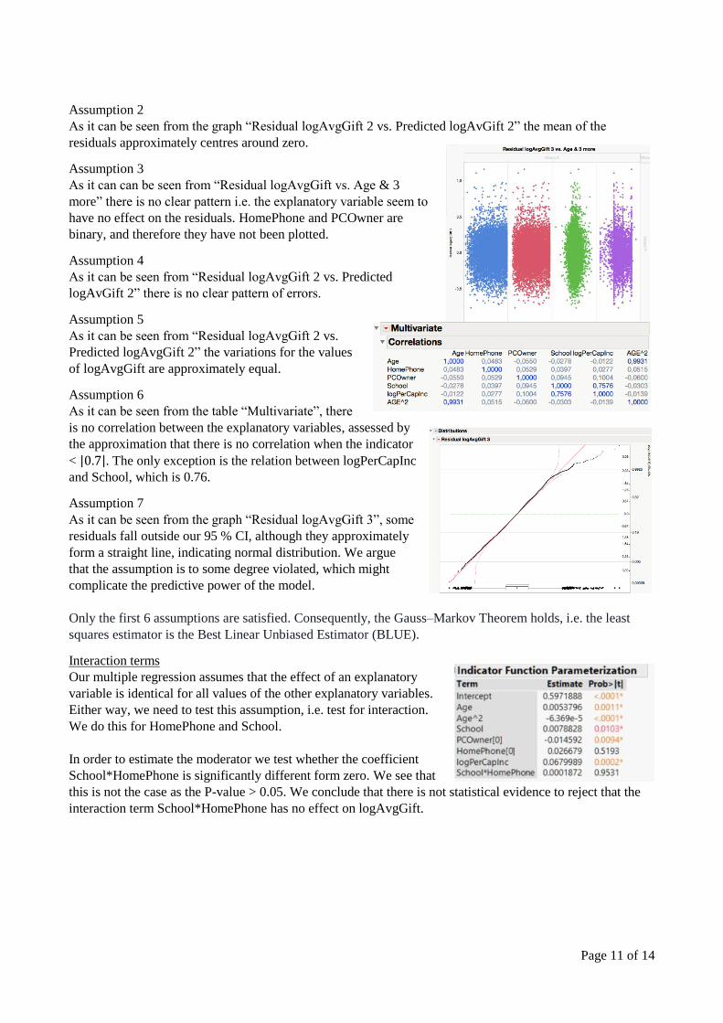
Assumption 2

As it can be seen from the graph “Residual logAvgGift 2 vs. Predicted logAvGift 2” the mean of the

residuals approximately centres around zero.

Assumption 3

As it can can be seen from “Residual logAvgGift vs. Age & 3

more” there is no clear pattern i.e. the explanatory variable seem to

have no effect on the residuals. HomePhone and PCOwner are

binary, and therefore they have not been plotted.

Assumption 4

As it can be seen from “Residual logAvgGift 2 vs. Predicted

logAvGift 2” there is no clear pattern of errors.

Assumption 5

As it can be seen from “Residual logAvgGift 2 vs.

Predicted logAvgGift 2” the variations for the values

of logAvgGift are approximately equal.

Assumption 6

As it can be seen from the table “Multivariate”, there

is no correlation between the explanatory variables, assessed by

the approximation that there is no correlation when the indicator

< |0.7|. The only exception is the relation between logPerCapInc

and School, which is 0.76.

Assumption 7

As it can be seen from the graph “Residual logAvgGift 3”, some

residuals fall outside our 95 % CI, although they approximately

form a straight line, indicating normal distribution. We argue

that the assumption is to some degree violated, which might

complicate the predictive power of the model.

Only the first 6 assumptions are satisfied. Consequently, the Gauss–Markov Theorem holds, i.e. the least

squares estimator is the Best Linear Unbiased Estimator (BLUE).

Interaction terms

Our multiple regression assumes that the effect of an explanatory

variable is identical for all values of the other explanatory variables.

Either way, we need to test this assumption, i.e. test for interaction.

We do this for HomePhone and School.

In order to estimate the moderator we test whether the coefficient

School*HomePhone is significantly different form zero. We see that

this is not the case as the P-value > 0.05. We conclude that there is not statistical evidence to reject that the

interaction term School*HomePhone has no effect on logAvgGift.

Page 12 of 14

(e) Explore whether the model can be improved by including any of the other “neighborhood”

variables (Professional, Technical, Farmers, etc.).

Now we include the explanatory variables; Technical, Professional and

Farmers to see, whether they improve our model. In JMP we generate the F-

ratio, the t-tests for each variable and the adjusted R2.

In our extended model, we get an R2 of 0.021057 and an adjusted R2 of

0.020106. In our previous model, our R2 is 0.020393 and our adjusted

R2 is 0.019759, which are both slightly smaller than our extended

model. Adding more explanatory variables artificially increase both R2

and adjusted R2. None of the new variables in our extended model is

statistically significant in a t-test, therefore we assess that we should

not include professional, farmers and technical.

Question 6 We now wish to build a model for predicting DidDonate.

(a) Fit a logistic regression model predicting DidDonate from Promotions. Compute the odds ratio

corresponding to each additional 10 promotions and give a 95% confidence interval for this odds ratio.

Logistic regression model predicting DidDonate from Promotions

We use a logistic regression model, when our response variable is categorical (here, TRUE and FALSE).

DidDonate is a dummy variable with the binary outcome of 1 and 0. Since the logistic model predicts the

probability of success, P must be 1 or 0. Therefore, we do not use the Ordinary Least Squares (OLS) method,

but the Maximum Likelihood Estimate (MLE) method.

The logistic regression equation in our model follows:

𝑃(𝐷𝑖𝑑𝐷𝑜𝑛𝑎𝑡𝑒 = 1 | 𝑥) =𝑒𝛽0+𝛽1𝑥

1+ 𝑒𝛽0+𝛽1𝑥.

The shape of the regression becomes more realistic as an S-shape than as a linear

trend. This gives us a logistic regression model predicting DidDonate from Promotions:

𝑃(𝐷𝑖𝑑𝐷𝑜𝑛𝑎𝑡𝑒 = 1 | 𝑥) = 𝑒−3.409+0.009∗𝑥

1+ 𝑒−3.409+0.009∗𝑥

For instance, the probability of donating, when having received 50 promotions would be:

𝑃(𝐷𝑖𝑑𝐷𝑜𝑛𝑎𝑡𝑒 | 50) =𝑒−3.409+0.009∗50

1+ 𝑒−3.409+0.009∗50 = 0.04931

The odds ratio corresponding to each additional 10 promotions

To compute the odds ratio corresponding to each additional 10 promotions, we continue with our example of

the probability of a respondent donating when having received 50 promotions:

𝑂𝑑𝑑𝑠(𝐷𝑖𝑑𝐷𝑜𝑛𝑎𝑡𝑒 = 1 | 50) =𝑃(𝐷𝑖𝑑𝐷𝑜𝑛𝑎𝑡𝑒=1 | 50)

1−𝑃(𝐷𝑖𝑑𝐷𝑜𝑛𝑎𝑡𝑒=1 | 50)=

0.04931

1−0.04931= 0.05187

We find the probability of a respondent donating when having received 60 promotions:

𝑂𝑑𝑑𝑠(𝐷𝑖𝑑𝐷𝑜𝑛𝑎𝑡𝑒 = 1 | 60) =𝑃(𝐷𝑖𝑑𝐷𝑜𝑛𝑎𝑡𝑒=1 | 60)

1−𝑃(𝐷𝑖𝑑𝐷𝑜𝑛𝑎𝑡𝑒=1 | 60)=

0.05371

1−0.05371= 0.05676

We compute the odds ratio between the two:

𝑂𝑅 =𝑂𝑑𝑑𝑠(𝐷𝑖𝑑𝐷𝑜𝑛𝑎𝑡𝑒=1 | 60)

𝑂𝑑𝑑𝑠(𝐷𝑖𝑑𝐷𝑜𝑛𝑎𝑡𝑒=1 | 50)=

0.05676

0.05187= 1.09427

Hence, the odds of donating are 1.09427 times more likely for each 10 promotions a person receives.

Page 13 of 14

Confidence interval for the odds ratio

The 95 % CI for the odds ratio:

𝐶𝐼(𝑂𝑅) = 𝑂𝑅 ± 1.96 ∗ 𝑠𝑒, where 𝑠𝑒 is found in the standard error of promotions from JMP

𝐶𝐼(𝑂𝑅) = 1.09427 ± 1.96 ∗ 0.00226 = [1.08984; 1.09869]

We are 95 % confident that the odds ratio will be between 1.08984 and 1.09869. Since this CI does not

contain 1, we are 95 % confident that promotions have a statistically significant effect on donations (and

since both odds ratios are above 1, this effect is positive). However, as these values are close to 1, the effect

of receiving each additional 10 promotions is small.

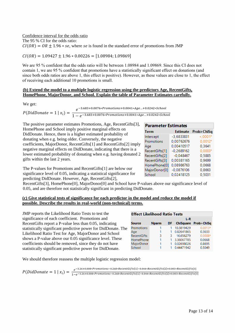
(b) Extend the model to a multiple logistic regression using the predictors Age, RecentGifts,

HomePhone, MajorDonor, and School. Explain the table of Parameter Estimates carefully.

We get:

𝑃(𝐷𝑖𝑑𝐷𝑜𝑛𝑎𝑡𝑒 = 1 | 𝑥𝑖) = 𝑒−3.683+0.0076∗𝑃𝑟𝑜𝑚𝑜𝑡𝑖𝑜𝑛𝑠+0.0041∗𝐴𝑔𝑒…+0.0242∗𝑆𝑐ℎ𝑜𝑜𝑙

1 − 𝑒−3.683+0.0076∗𝑃𝑟𝑜𝑚𝑜𝑡𝑖𝑜𝑛𝑠+0.0041∗𝐴𝑔𝑒…+0.0242∗𝑆𝑐ℎ𝑜𝑜𝑙

The positive parameter estimates Promotions, Age, RecentGifts[3],

HomePhone and School imply positive marginal effects on

DidDonate. Hence, there is a higher estimated probability of

donating when e.g. being older. Conversely, the negative

coefficients, MajorDonor, RecentGifts[1] and RecentGifts[2] imply

negative marginal effects on DidDonate, indicating that there is a

lower estimated probability of donating when e.g. having donated 2

gifts within the last 2 years.

The P-values for Promotions and RecentGifts[1] are below our

significance level of 0.05, indicating a statistical significance for

predicting DidDonate. However, Age, RecentGifts[2],

RecentGifts[3], HomePhone[0], MajorDonor[0] and School have P-values above our significance level of

0.05, and are therefore not statistically significant in predicting DidDonate.

(c) Give statistical tests of significance for each predictor in the model and reduce the model if

possible. Describe the results in real-world (non-technical) terms.

JMP reports the Likelihood Ratio Tests to test the

significance of each coefficient. Promotions and

RecentGifts report a P-value less than 0.05, indicating

statistically significant predictive power for DidDonate. The

Likelihood Ratio Test for Age, MajorDonor and School

shows a P-value above our 0.05 significance level. These

coefficients should be removed, since they do not have

statistically significant predictive power for DidDonate.

We should therefore reassess the multiple logistic regression model:

𝑃(𝐷𝑖𝑑𝐷𝑜𝑛𝑎𝑡𝑒 = 1 | 𝑥𝑖) = 𝑒−3.26+0.008∗𝑃𝑟𝑜𝑚𝑜𝑡𝑖𝑜𝑛𝑠−0.268∗𝑅𝑒𝑐𝑒𝑛𝑡𝐺𝑖𝑓𝑡𝑠[1]−0.044∗𝑅𝑒𝑐𝑒𝑛𝑡𝐺𝑖𝑓𝑡𝑠[2]+0.003∗𝑅𝑒𝑐𝑒𝑛𝑡𝐺𝑖𝑓𝑡𝑠[3]

1−𝑒−3.26+0.008∗𝑃𝑟𝑜𝑚𝑜𝑡𝑖𝑜𝑛𝑠−0.268∗𝑅𝑒𝑐𝑒𝑛𝑡𝐺𝑖𝑓𝑡𝑠[1]−0.044∗𝑅𝑒𝑐𝑒𝑛𝑡𝐺𝑖𝑓𝑡𝑠[2]+0.003∗𝑅𝑒𝑐𝑒𝑛𝑡𝐺𝑖𝑓𝑡𝑠[3]

Page 14 of 14

In real world terms, this means that the number of promotions received before

the mailings, and the amounts of gifts given beforehand, do have a say in

whether a person donated or not. Specifically, the number of promotions you

have received have a positive effect on donating after receiving the mailing.

Having donated one gift within the last two years has a negative effect on the

donating after receiving the mailing. Having donated two gifts in the last two

years also has a negative effect. However, having donated three gifts within the

last two years has a positive (but small) effect on donating after receiving the

mailing.

A person’s age, whether they own a home phone, whether they have a major donor in their neighbourhood,

and how many years of school the average person in their neighbourhood has received, do not influence the

likelihood of donating after receiving the mailing.