Embed Size (px)
Citation preview
Statistics and Quantitative RiskManagement for Banking and In-surance
Paul EmbrechtsRiskLab, Department of Mathematics and Swiss Finance Institute, ETHZurich, 8092 Zurich, Switzerland, [email protected]
Marius HofertRiskLab, Department of Mathematics, ETH Zurich, 8092 Zurich, Switzerland,[email protected]. The author (Willis Research Fellow) thanksWillis Re for financial support while this work was being completed.
KeywordsStatistical methods, risk measures, dependence modeling, risk aggregation,regulatory practice
AbstractAs an emerging field of applied research, Quantitative Risk Management(QRM) poses a lot of challenges for probabilistic and statistical modeling.This review provides a discussion on selected past, current, and possiblefuture areas of research in the intersection of statistics and quantitative riskmanagement. Topics treated include the use of risk measures in regulation,including their statistical estimation and aggregation properties. An extensiveliterature provides the statistically interested reader with an entrance to thisexciting field.
www.annualreviews.org • Statistics and Quantitative Risk Management for Banking and Insurance 1
1. IntroductionIn 2005, the first author (Paul Embrechts), together with Alexander J. McNeiland Rüdiger Frey, wrote the by now well-established text McNeil et al. (2005).Whereas the title read as “Quantitative Risk Management: Concepts, Tech-niques, Tools”, a somewhat more precise description of the content would bereflected in “Statistical Methods for Quantitative Risk Management: Con-cepts, Techniques, Tools”. Now, almost a decade and several financial criseslater, more than ever, the topic of Quantitative Risk Management (QRM) ishigh on the agenda of academics, practitioners, regulators, politicians, the media,as well as the public at large. The current paper aims at giving a brief historicaloverview of how QRM as a field of statistics and applied probability came to be.We will discuss some of its current themes of research and attempt to summarize(some of) the main challenges going forward. This is not an easy task as theword “risk” is omnipresent in modern society and consequently its (statistical)quantification. One therefore has to be careful not to lose sight of the forestfor the trees! Under the heading “QRM: The Nature of the Challenge”, inMcNeil et al. (2005, Section 1.5.1) it is written: “We set ourselves the task ofdefining a new discipline of QRM and our approach to this task has two mainstrands. On the one hand, we have attempted to put current practice onto afirmer mathematical footing. On the other hand, the second strand of ourendeavor has been to put together material on techniques and tools which gobeyond current practice and address some of the deficiencies that have beenraised repeatedly by critics”. Especially in the wake of financial crises, it isnot always straightforward to defend a more mathematical approach on “risk”(more on this later). For the purpose of the paper, we interpret risk at the moremathematical level of (random) uncertainty in both frequency as well as severityof loss events. We will not enter into the, very important, discussion around“Risk and Uncertainty” (Knight (1921)) on the various “Knowns, Unknowns andUnknowables” (Diebold et al. (2010)). Concerning “mathematical level”, letthe following quotes speak for themselves. First, in their (Nobel-)path breakingpaper Gale and Shapley (1962) are addressing the question “What is mathemat-ics?” the authors wrote “. . . any argument which is carried out with sufficientprecision is mathematical,. . . ”. Lloyd Shapley (together with Alvin Roth) gotthe 2012 Nobel Prize for economics; see Roth and Shapley (2012). As a secondquote on the topic we like Norbert Wiener’s; see Wiener (1923):
“Mathematics is an experimental science . . . It matters little . . .that the mathematician experiments with pencil and paper whilethe chemist uses test-tube and retort, or the biologist stains andthe microscope . . . The only great point of divergence betweenmathematics and other sciences lies in the far greater permanence ofmathematical knowledge, in the circumstance that experience onlywhispers ’yes’ or ’no’ in reply to our questions, while logic shouts.”
It is precisely statistics that has to straddle the shouting world of mathematicallogic with the whispering one of practical reality.
2 Paul Embrechts, Marius Hofert
2. A whisper from regulatory practice
In the financial (banking and insurance) industry, solvency regulation has beenaround for a long time. The catchwords are Basel for banking and Solvency forinsurance. The former derives from the Basel Committee on Banking Supervision,a supra-national institution, based in Basel, Switzerland, working out solvencyguidelines for banks. Basic frameworks go under the names of Basel I, II, IIItogether with some intermediate stages. The website www.bis.org/bcbs ofthe Bank for International Settlements (BIS) warrants a regular visit fromanyone interested in banking regulation. An excellent historic overview of theCommittee’s working is to be found in Tarullo (2008). Similar developments forthe insurance industry go under the name of Solvency, in particular the currentSolvency II framework. For a broader overview, see Sandström (2006). WhereasSolvency II is not yet in force, since January 1, 2011, the Swiss Solvency Test(SST) is. The key principles on which the SST, originating in 2003, is based are:(a) it is risk based, quantifying market, insurance and credit risk, (b) it stressesmarket consistent valuation of assets and liabilities, and (c) advocates a totalbalance sheet approach. Before, actuaries were mainly involved with liabilitypricing and reserve calculations. Within the SST, stress scenarios are to bequantified and aggregated for capital requirement. Finally, as under the Baselregime for banking, internal models are encouraged and need approval by therelevant regulators (the FINMA in the case of Switzerland). An interesting textexposing the main issues both from a more methodological as well as practicalpoint of view is SCOR (2008). As in any field of applications, if as a statisticianone really wants to have an impact one has to get more deeply involved withpractice. From this point of view, some of the above publications are must reads.McNeil et al. (2005, Chapter 1) gives a somewhat smooth introduction for thoselacking the necessary time.Let us concentrate on one particular example highlighting the potentially
interesting interactions between methodology and practice, and hence the title ofthis section. As already stated, the Basel Committee, on a regular basis, producesdocuments aimed at improving the resilience of the international financial system.The various stakeholders, including academia, are asked to comment on thesenew guidelines before they are submitted to the various national agencies to becast into local law. One such document is BIS (2012). In the latter consultativedocument, p. 41, the following question (Nr. 8) is asked: “What are the likelyoperational constraints with moving from VaR to ES, including any challengesin delivering robust backtesting, and how might these be best overcome?”; forVaR and ES, see Definition 2.1. This is an eminently statistical question themeaning of which, together with possible answers, we shall discuss below. Thisexample has to be viewed as a blueprint for similar discussions of statisticalnature within the current QRM landscape. Some further legal clarification maybe useful at this point: by issuing consultative documents, the Basel Committeewants to intensify its consultation and discussions with the various stakeholdersof the financial system. In particular, academia and industry are invited tocomment on the new proposals and as such may have an influence on the precise
www.annualreviews.org • Statistics and Quantitative Risk Management for Banking and Insurance 3
formulations going forward. The official replies are published on the websiteof the BIS. We will not be able to enter into all relevant details but merelyhighlight the issues relevant from a more statistical point of view; in doing so,we will make several simplifying assumptions.
The first ingredient is a portfolio P of financial positions each with a well-defined value at any time t. For t (today, say) the value of the portfolio is vt.Though crucial in practice, we will not enter into a more detailed economicand/or actuarial discussion of the precise meaning of value: it suffices to mentionpossibilities like “fair value”, “market value” (mark-to-market), “model value”(mark-to-model), “accounting value” (often depending on the jurisdiction underwhich industry is regulated) and indeed various combinations of the above!Viewed from today, the value of the portfolio one time period in the future isa random variable Vt+1. In (market) risk management one is interested in the(positive) tail of the so-called Profit-and-Loss (P&L) distribution function(df) of the random variable (rv)
Lt+1 = −(Vt+1 − vt). (1)
The one-period ahead value Vt+1 is determined by the structure S(t+ 1,Zt+1)of P , where Zt+1 in Rd is a (typically) high-dimensional random vector of riskfactors with corresponding risk-factor changes Xt+1 = Zt+1 − zt. S is alsoreferred to as the mapping. As an example consider for P a linear portfolioconsisting of βj stocks St,j, j ∈ {1, . . . , d} (St,j denotes the value of stock j attime t and βj the number of shares of stock j in P). Furthermore, assume therisk factors to be
Zt = (Zt,1, . . . , Zt,d), Zt,j = logSt,j
and the corresponding risk-factor changes to be the log-returns (here again, tdenotes today):
Xt+1 = log(St+1,j)− log(st,j) = log(St+1,j
st,j
).
In this case, the portfolio structure is
S(t+ 1,Zt+1) =d∑j=1
βjSt+1,j =d∑j=1
βj exp(Zt+1,j). (2)
(1) together with Vt+1 = S(t+ 1,Zt+1) then implies that
Lt+1 = −d∑j=1
βj(exp(Zt+1,j)− exp(zt,j))
= −d∑j=1
βj(exp(zt,j +Xt+1,j)− exp(zt,j)) = −d∑j=1
wt,j(exp(Xt+1,j)− 1),
where wt,j = βjst,j; wt,j = wt,j/vt is then the relative value of stock j in P . Forthis, and further examples, see McNeil et al. (2005, Section 2.1.3).
4 Paul Embrechts, Marius Hofert
Based on models and statistical estimates (computed from data) for (Xt+1),the problem is now clear: find the df (or some characteristic, a risk measure) ofLt+1. Here, “the df” can be interpreted unconditionally or conditionally on somefamily of σ-algebras (a filtration of historical information). As a consequence,the mathematical set-up can become arbitrarily involved!Analytically, (1) becomes
Lt+1 = −(S(t+ 1,Zt+1)− S(t, zt))= −(S(t+ 1, zt + Xt+1)− S(t, zt)). (3)
If, for ease of notation, we suppress the time dependence, (3) becomes
L = −(S(z + X)− S(z)) (4)
with z ∈ Rd and X a d-dimensional random vector denoting the one-periodchanges in factor values; d is typically high, d ≥ 1000! In general, the functionS can be highly non-linear. This especially holds true in cases where derivativefinancial instruments (like options) are involved. If time is modeled explicitly(which in practice is necessary) then (3) is a time series (Lt)t (stationary ornot) driven by a d-dimensional stochastic process (Xt)t and a deterministic,though mostly highly non-linear portfolio structure S. Going back (for easeof notation) to the static case (4), one has to model the df FL(x) = P(L ≤ x)under various assumptions on the input. Only for the most trivial case, like Xis multivariate normal and S linear, can this be handled analytically. In practice,various approximation methods are used:(A1) Replace S by a linearized version S∆ using Taylor expansion and approxi-
mate FL by the df FL∆ of the linearized loss L∆; here one uses smoothnessof S (usually fine) combined with a condition that X in (4) is stochasticallysmall (a more problematic assumption). The latter implies that one-periodchanges in the risk factors are small; this is acceptable in “normal” periodsbut not in “extreme” periods. Note that it is especially for the latter thatQRM is needed!
(A2) Find stochastic models for (Xt)t closer to reality, in particular beyondGaussianity but for which FL or FL∆ can be calculated/estimated readily.This is a non-trivial task in general.
(A3) Rather than aiming for a full model for FL, estimate some characteristicsof FL relevant for solvency capital calculations, that is, estimate a so-calledrisk measure. Here the VaR and ES abbreviations in the above BIS(2012) quote enter, both are risk measures; they are defined as follows.
Definition 2.1Suppose L as given above and let 0 < α < 1, theni) The Value-at-Risk of L at confidence level α is given by
VaRα(L) = inf{x ∈ R : FL(x) ≥ α}
(i.e. VaRα(L) is the 100α% quantile of FL).
www.annualreviews.org • Statistics and Quantitative Risk Management for Banking and Insurance 5
ii) The Expected Shortfall of L at confidence level α is given by
ESα(L) = 11− α
∫ 1
αVaRu(L) du.
Remark 2.21) VaRα(L) defined above coincides with the so-called generalized inverse
F←L (α) at the confidence level α; see Embrechts and Hofert (2013a). Itsintroduction around 1994, linked to (4) as a basis for solvency capital calcu-lation, truly led to a new risk management benchmark on Wall Street; seeJorion (2007). A simple Google search will quickly confirm this. An inter-esting text aiming at improving VaR-usage and warning about the variousmisunderstandings and misuses is Wong (2013).
2) For FL continuous, the definition of Expected Shortfall is equivalent to
ESα(L) = E[L |L > VaRα(L)],
hence its name. Alternative names in use throughout the financial industryare “conditional VaR” and “conditional tail expectation”.
3) Note that ES does not exist for infinite mean models, i.e. when ESα |L| =∞.This reveals a potential problem with ES as a risk measure in case of veryheavy-tailed loss data.
4) Both risk measures are used in industry and regulation; VaR more in banking,ES more in insurance, the latter especially under the SST. Depending on therisk class under consideration, different values of α (typically close to 1) andthe holding period (“the one period” above, see (1)) are in use; see McNeilet al. (2005) for details.
5) A whole industry of papers on estimating VaR and/or ES has emerged,and this under a wide variety of model assumptions on the underlying P&Lprocess (Lt)t. McNeil et al. (2005) contains a summary of results stressing themore statistical issues. An excellent companion text with a more econometricflavour is Daníelsson (2011). More recent statistical techniques in use are forinstance extreme quantile estimation based on regime-switching models andlasso-technology, see Chavez-Demoulin et al. (2013a). Estimation based onself-exciting (or Hawkes) processes is exemplified in Chavez-Demoulin andMcGill (2012). For an early use on Hawkes processes in finance, see Chavez-Demoulin et al. (2005). McNeil et al. (2005, Section 7.4.3) contains an earlytext-book reference to QRM. Extreme Value Theory (EVT) methodology isfor instance presented in McNeil and Frey (2000); Chavez-Demoulin et al.(2013b) use it in combination with generalized additive models in order tomodel VaR for Operational Risk based on covariates.
6) From the onset, especially VaR has been heavily criticized as it only looksat the frequency of extremal losses (α close to 1) but not at the severity.The important “what if” question is more addressed by ES. Furthermore,in general VaR is not a subadditive risk measure, i.e. it is possible that
6 Paul Embrechts, Marius Hofert
for two positions L1 and L2, VaRα(L1 + L2) > VaRα(L1) + VaRα(L2) forsome 0 < α < 1. This makes risk aggregation and diversification argumentsdifficult. ES as defined in Definition 2.1 ii) above is always subadditive. Theseissues played a role in the subprime crisis of 2007–2009; see Donnelly andEmbrechts (2010) and Das et al. (2013) for some discussions on this. McNeilet al. (2005) contains an in-depth analysis together with numerous referencesfor further reading. Whereas industry early on (mid nineties) did not reallytake notice of the warnings concerning the problem with VaR in marketsaway from “normality”, by now the negative issues underlying VaR-basedregulation have become abundantly clear and the literature is full of exampleson this. Below we have included a particular example from the realm ofcredit risk stressing, hopefully exposing in a pedagogically clear way, someof the problems. It is a slightly expanded version of McNeil et al. (2005,Example 6.7) and basically goes back to Albanese (1997). By now, thereexist numerous similar examples.
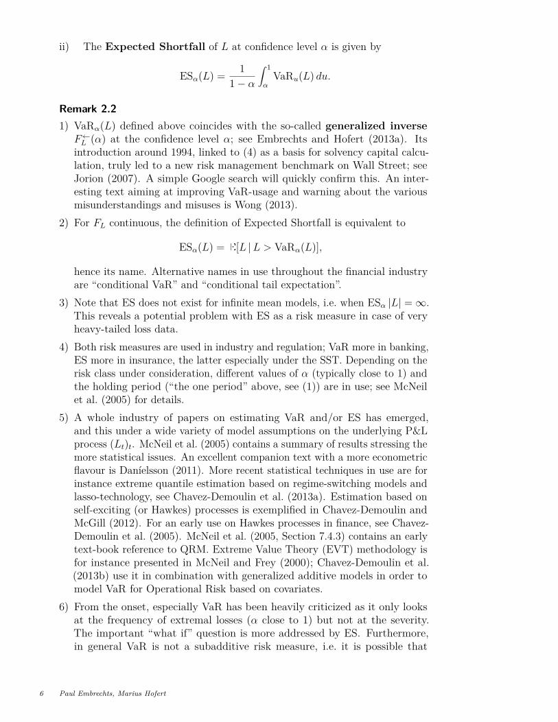
Example 2.3 (Non-subadditivity of VaR)Assume we have given 100 bonds with maturity T equal to one year, nominalvalue 100, yearly coupon 2%, and default probability 1% (no recovery). Thecorresponding losses (assumed to be independent) are
Li =
−2, with probability 0.99,100, with probability 0.01,
i ∈ {1, . . . , 100}.
(Recall the choice of negative values to denote gains!) Consider two portfolios,
P1 :100∑i=1
Li and P2 : 100L1. (5)
P1 is a so-called diversified portfolio and P2 clearly a highly concentrated one.As this point the reader may judge for himself/herself which of the two portfolioshe/she believes to be less risky (and thus would assign a smaller risk measureto).
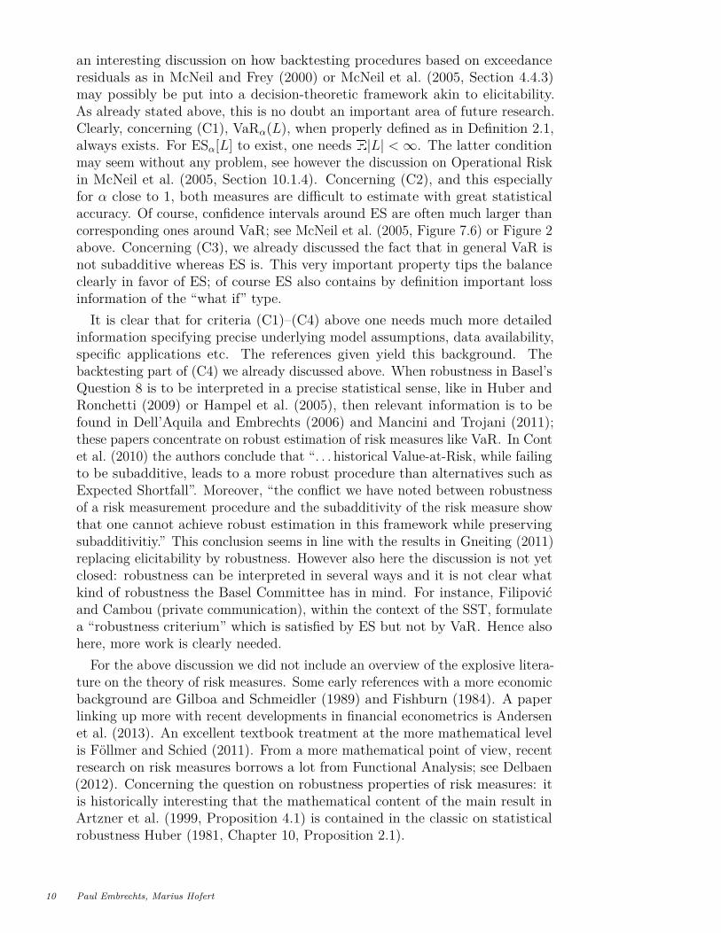
Figure 1 shows the boundaries of this decision according to VaR (the shift by201 in y scale is for plotting the y axis in log-scale). Rather surprisingly, forα = 0.95, for example, VaRα is superadditive, i.e.
VaR0.95(P1) > VaR0.95(P2).
By the interpretation of a risk measure as the amount of capital required asa buffer against future losses, this implies that the diversified portfolio P1can be riskier (thus requiring a larger risk capital) than the concentrated P2according to VaR. Indeed, one can show that for two portfolios as in (5) basedon n bonds with default probability p, VaRα is superadditive if and only if(1 − p)n < α ≤ 1 − p. This formula holds independently of the coupon andnominal value. For n = 100 and p = 1% we obtain that VaRα is superadditive ifand only if 0.3660 ≈ 0.99100 < α ≤ 0.99.
www.annualreviews.org • Statistics and Quantitative Risk Management for Banking and Insurance 7
0.0 0.2 0.4 0.6 0.8 1.0
110
100
1000
1000
0
VaRα(L1 + … + L100) vs ∑i=1
100VaRα(Li) for Example 2.3
α
VaR
α+
201
VaRα(L1 + … + L100)
∑i=1
100
VaRα(Li)
Figure 1V aRα as a function in α for the two portfolios P1 and P2.
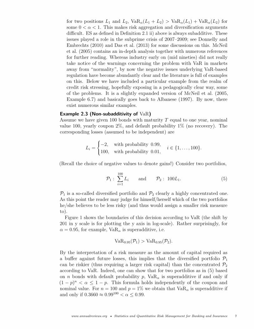
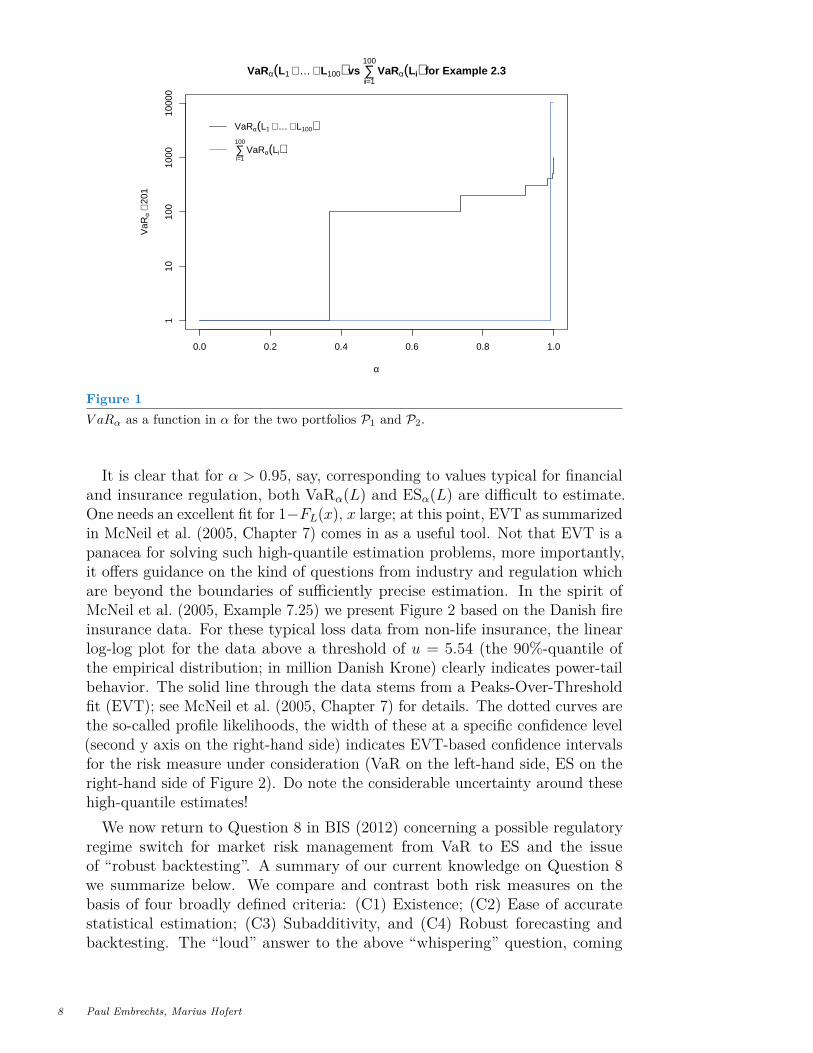
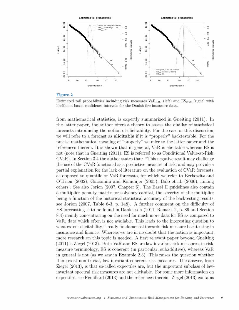
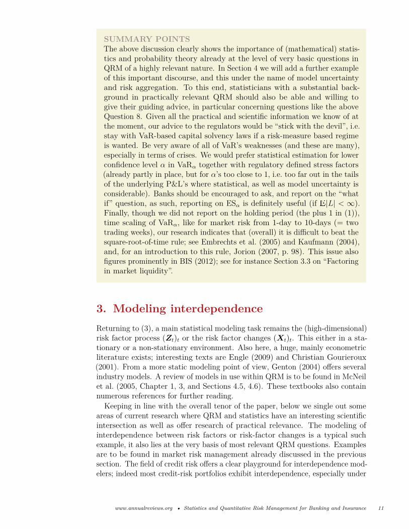
It is clear that for α > 0.95, say, corresponding to values typical for financialand insurance regulation, both VaRα(L) and ESα(L) are difficult to estimate.One needs an excellent fit for 1−FL(x), x large; at this point, EVT as summarizedin McNeil et al. (2005, Chapter 7) comes in as a useful tool. Not that EVT is apanacea for solving such high-quantile estimation problems, more importantly,it offers guidance on the kind of questions from industry and regulation whichare beyond the boundaries of sufficiently precise estimation. In the spirit ofMcNeil et al. (2005, Example 7.25) we present Figure 2 based on the Danish fireinsurance data. For these typical loss data from non-life insurance, the linearlog-log plot for the data above a threshold of u = 5.54 (the 90%-quantile ofthe empirical distribution; in million Danish Krone) clearly indicates power-tailbehavior. The solid line through the data stems from a Peaks-Over-Thresholdfit (EVT); see McNeil et al. (2005, Chapter 7) for details. The dotted curves arethe so-called profile likelihoods, the width of these at a specific confidence level(second y axis on the right-hand side) indicates EVT-based confidence intervalsfor the risk measure under consideration (VaR on the left-hand side, ES on theright-hand side of Figure 2). Do note the considerable uncertainty around thesehigh-quantile estimates!We now return to Question 8 in BIS (2012) concerning a possible regulatory
regime switch for market risk management from VaR to ES and the issueof “robust backtesting”. A summary of our current knowledge on Question 8we summarize below. We compare and contrast both risk measures on thebasis of four broadly defined criteria: (C1) Existence; (C2) Ease of accuratestatistical estimation; (C3) Subadditivity, and (C4) Robust forecasting andbacktesting. The “loud” answer to the above “whispering” question, coming
8 Paul Embrechts, Marius Hofert
●●●●●●●●●●●●●●●●●●●●●●●●●●●●●●●●●●●●●●●●●●●●●●●●●●●●●●●●●●●●●●●●●●●●●●●●●●●●●●●●●●●●●●●●●●●●●●●●●●●●●●●●●●●●●●●●●●●●●●●●●●●●●●●●●●●●●●●●●●●●●●●●●●●●●●●●●●●●●●●●●●●●●●●●●●●●●●●●●●●●●●●●●●●●●●●●●●●●●●●●●●●●●●
●●
●●
●●●
●
●
●
●
5 10 20 50 100 200
2e−
041e
−03
5e−
032e
−02
1e−
01
Estimated tail probabilities
Exceedances x
1−
Fn(x
)
0.99
50.
990.
950.
90.
80.
5
Con
fiden
ce in
terv
als
GPD(0.58, 4.51) tail estimateVaR0.99 estimate (= 27.45)VaR0.99 CIs
●●●●●●●●●●●●●●●●●●●●●●●●●●●●●●●●●●●●●●●●●●●●●●●●●●●●●●●●●●●●●●●●●●●●●●●●●●●●●●●●●●●●●●●●●●●●●●●●●●●●●●●●●●●●●●●●●●●●●●●●●●●●●●●●●●●●●●●●●●●●●●●●●●●●●●●●●●●●●●●●●●●●●●●●●●●●●●●●●●●●●●●●●●●●●●●●●●●●●●●●●●●●●●
●●
●●
●●●
●
●
●
●
5 10 20 50 100 200
2e−
041e
−03
5e−
032e
−02
1e−
01
Estimated tail probabilities
Exceedances x
1−
Fn(x
)
0.99
50.
950.
90.
80.
5
Con
fiden
ce in
terv
als
GPD(0.58, 4.51) tail estimateES0.99 estimate (= 69.02)ES0.99 CIs
Figure 2Estimated tail probabilities including risk measures VaR0.99 (left) and ES0.99 (right) withlikelihood-based confidence intervals for the Danish fire insurance data.
from mathematical statistics, is expertly summarized in Gneiting (2011). Inthe latter paper, the author offers a theory to assess the quality of statisticalforecasts introducing the notion of elicitability. For the ease of this discussion,we will refer to a forecast as elicitable if it is “properly” backtestable. For theprecise mathematical meaning of “properly” we refer to the latter paper and thereferences therein. It is shown that in general, VaR is elicitable whereas ES isnot (note that in Gneiting (2011), ES is referred to as Conditional Value-at-Risk,CVaR). In Section 3.4 the author states that: “This negative result may challengethe use of the CVaR functional as a predictive measure of risk, and may provide apartial explanation for the lack of literature on the evaluation of CVaR forecasts,as opposed to quantile or VaR forecasts, for which we refer to Berkowitz andO’Brien (2002), Giacomini and Komunjer (2005), Balo et al. (2006), amongothers”. See also Jorion (2007, Chapter 6). The Basel II guidelines also containa multiplier penalty matrix for solvency capital, the severity of the multiplierbeing a function of the historical statistical accuracy of the backtesting results;see Jorion (2007, Table 6-3, p. 148). A further comment on the difficulty ofES-forecasting is to be found in Daníelsson (2011, Remark 2, p. 89 and Section8.4) mainly concentrating on the need for much more data for ES as compared toVaR, data which often is not available. This leads to the interesting question towhat extent elicitability is really fundamental towards risk-measure backtesting ininsurance and finance. Whereas we are in no doubt that the notion is important,more research on this topic is needed. A first relevant paper beyond Gneiting(2011) is Ziegel (2013). Both VaR and ES are law invariant risk measures, in risk-measure terminology, ES is coherent (in particular, subadditive), whereas VaRin general is not (as we saw in Example 2.3). This raises the question whetherthere exist non-trivial, law-invariant coherent risk measures. The answer, fromZiegel (2013), is that so-called expectiles are, but the important subclass of law-invariant spectral risk measures are not elicitable. For some more information onexpectiles, see Rémillard (2013) and the references therein. Ziegel (2013) contains
www.annualreviews.org • Statistics and Quantitative Risk Management for Banking and Insurance 9
an interesting discussion on how backtesting procedures based on exceedanceresiduals as in McNeil and Frey (2000) or McNeil et al. (2005, Section 4.4.3)may possibly be put into a decision-theoretic framework akin to elicitability.As already stated above, this is no doubt an important area of future research.Clearly, concerning (C1), VaRα(L), when properly defined as in Definition 2.1,always exists. For ESα[L] to exist, one needs E|L| <∞. The latter conditionmay seem without any problem, see however the discussion on Operational Riskin McNeil et al. (2005, Section 10.1.4). Concerning (C2), and this especiallyfor α close to 1, both measures are difficult to estimate with great statisticalaccuracy. Of course, confidence intervals around ES are often much larger thancorresponding ones around VaR; see McNeil et al. (2005, Figure 7.6) or Figure 2above. Concerning (C3), we already discussed the fact that in general VaR isnot subadditive whereas ES is. This very important property tips the balanceclearly in favor of ES; of course ES also contains by definition important lossinformation of the “what if” type.It is clear that for criteria (C1)–(C4) above one needs much more detailed
information specifying precise underlying model assumptions, data availability,specific applications etc. The references given yield this background. Thebacktesting part of (C4) we already discussed above. When robustness in Basel’sQuestion 8 is to be interpreted in a precise statistical sense, like in Huber andRonchetti (2009) or Hampel et al. (2005), then relevant information is to befound in Dell’Aquila and Embrechts (2006) and Mancini and Trojani (2011);these papers concentrate on robust estimation of risk measures like VaR. In Contet al. (2010) the authors conclude that “. . . historical Value-at-Risk, while failingto be subadditive, leads to a more robust procedure than alternatives such asExpected Shortfall”. Moreover, “the conflict we have noted between robustnessof a risk measurement procedure and the subadditivity of the risk measure showthat one cannot achieve robust estimation in this framework while preservingsubadditivitiy.” This conclusion seems in line with the results in Gneiting (2011)replacing elicitability by robustness. However also here the discussion is not yetclosed: robustness can be interpreted in several ways and it is not clear whatkind of robustness the Basel Committee has in mind. For instance, Filipovićand Cambou (private communication), within the context of the SST, formulatea “robustness criterium” which is satisfied by ES but not by VaR. Hence alsohere, more work is clearly needed.
For the above discussion we did not include an overview of the explosive litera-ture on the theory of risk measures. Some early references with a more economicbackground are Gilboa and Schmeidler (1989) and Fishburn (1984). A paperlinking up more with recent developments in financial econometrics is Andersenet al. (2013). An excellent textbook treatment at the more mathematical levelis Föllmer and Schied (2011). From a more mathematical point of view, recentresearch on risk measures borrows a lot from Functional Analysis; see Delbaen(2012). Concerning the question on robustness properties of risk measures: itis historically interesting that the mathematical content of the main result inArtzner et al. (1999, Proposition 4.1) is contained in the classic on statisticalrobustness Huber (1981, Chapter 10, Proposition 2.1).
10 Paul Embrechts, Marius Hofert
SUMMARY POINTSThe above discussion clearly shows the importance of (mathematical) statis-tics and probability theory already at the level of very basic questions inQRM of a highly relevant nature. In Section 4 we will add a further exampleof this important discourse, and this under the name of model uncertaintyand risk aggregation. To this end, statisticians with a substantial back-ground in practically relevant QRM should also be able and willing togive their guiding advice, in particular concerning questions like the aboveQuestion 8. Given all the practical and scientific information we know of atthe moment, our advice to the regulators would be “stick with the devil”, i.e.stay with VaR-based capital solvency laws if a risk-measure based regimeis wanted. Be very aware of all of VaR’s weaknesses (and these are many),especially in terms of crises. We would prefer statistical estimation for lowerconfidence level α in VaRα together with regulatory defined stress factors(already partly in place, but for α’s too close to 1, i.e. too far out in the tailsof the underlying P&L’s where statistical, as well as model uncertainty isconsiderable). Banks should be encouraged to ask, and report on the “whatif” question, as such, reporting on ESα is definitely useful (if E|L| < ∞).Finally, though we did not report on the holding period (the plus 1 in (1)),time scaling of VaRα, like for market risk from 1-day to 10-days (= twotrading weeks), our research indicates that (overall) it is difficult to beat thesquare-root-of-time rule; see Embrechts et al. (2005) and Kaufmann (2004),and, for an introduction to this rule, Jorion (2007, p. 98). This issue alsofigures prominently in BIS (2012); see for instance Section 3.3 on “Factoringin market liquidity”.
3. Modeling interdependenceReturning to (3), a main statistical modeling task remains the (high-dimensional)risk factor process (Zt)t or the risk factor changes (Xt)t. This either in a sta-tionary or a non-stationary environment. Also here, a huge, mainly econometricliterature exists; interesting texts are Engle (2009) and Christian Gourieroux(2001). From a more static modeling point of view, Genton (2004) offers severalindustry models. A review of models in use within QRM is to be found in McNeilet al. (2005, Chapter 1, 3, and Sections 4.5, 4.6). These textbooks also containnumerous references for further reading.
Keeping in line with the overall tenor of the paper, below we single out someareas of current research where QRM and statistics have an interesting scientificintersection as well as offer research of practical relevance. The modeling ofinterdependence between risk factors or risk-factor changes is a typical suchexample, it also lies at the very basis of most relevant QRM questions. Examplesare to be found in market risk management already discussed in the previoussection. The field of credit risk offers a clear playground for interdependence mod-elers; indeed most credit-risk portfolios exhibit interdependence, especially under
www.annualreviews.org • Statistics and Quantitative Risk Management for Banking and Insurance 11
extreme market conditions. The various financial crises (subprime, sovereign,. . . )give ample of proof. For instance the famous AAA-guarantee given by therating agencies for the (super-)senior tranches of Collateralized Debt Obligations(CDOs) turned out to be well below this low-risk level when the Americanhousing marked collapsed around 2006. An early warning for the consequencesof even a slight increase in interdependence between default-events of creditpositions for the evaluation of securitized products like CDOs is to be found inMcNeil et al. (2005, Figure 8.1); see also Hofert and Scherer (2011). The biggermethodological umbrella to be put over such examples is Model Uncertainty.The latter is no doubt one of the most active and practically relevant researchfields in QRM at the moment. We shall only highlight some aspects below,starting first with the notion of copula.In the late nineties, the concept of copula took QRM by storm. A copula
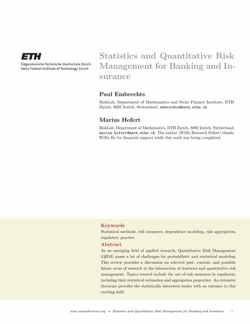
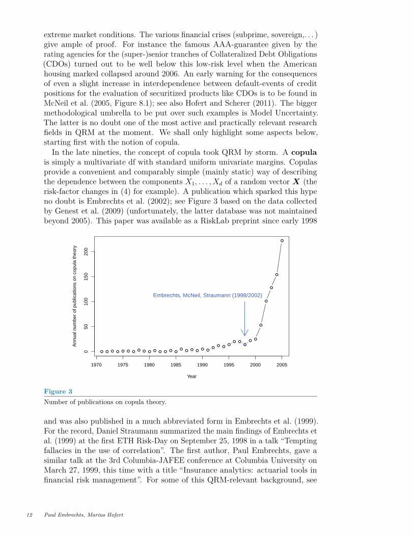
is simply a multivariate df with standard uniform univariate margins. Copulasprovide a convenient and comparably simple (mainly static) way of describingthe dependence between the components X1, . . . , Xd of a random vector X (therisk-factor changes in (4) for example). A publication which sparked this hypeno doubt is Embrechts et al. (2002); see Figure 3 based on the data collectedby Genest et al. (2009) (unfortunately, the latter database was not maintainedbeyond 2005). This paper was available as a RiskLab preprint since early 1998
● ● ● ● ● ● ●● ● ● ● ● ● ● ●
●● ● ●
● ●●
● ●●
● ●●
●●
●
●
●
●
●
1970 1975 1980 1985 1990 1995 2000 2005
050
100
150
200
Year
Ann
ual n
umbe
r of
pub
licat
ions
on
copu
la th
eory
●
Embrechts, McNeil, Straumann (1998/2002)
Figure 3Number of publications on copula theory.
and was also published in a much abbreviated form in Embrechts et al. (1999).For the record, Daniel Straumann summarized the main findings of Embrechts etal. (1999) at the first ETH Risk-Day on September 25, 1998 in a talk “Temptingfallacies in the use of correlation”. The first author, Paul Embrechts, gave asimilar talk at the 3rd Columbia-JAFEE conference at Columbia University onMarch 27, 1999, this time with a title “Insurance analytics: actuarial tools infinancial risk management”. For some of this QRM-relevant background, see
12 Paul Embrechts, Marius Hofert
Donnelly and Embrechts (2010). We would like to stress, however, that thecopula concept has been around almost for as long as modern probability andstatistics emerged in the early 20th century. Related work can be traced back toFréchet (1935) and Hoeffding (1940), for example.The central theorem underlying the theory and applications of copulas is
Sklar’s Theorem; see Sklar (1959). It consists of two parts. The first onestates that for any multivariate df H with margins F1, . . . , Fd, there exists acopula C such that
H(x1, . . . , xd) = C(F1(x1), . . . , Fd(xd)), x ∈ Rd. (6)
This decomposition is not necessarily unique, but it is in the case where all mar-gins F1, . . . , Fd are continuous. The second part provides a converse statement:Given any copula C and univariate dfs F1, . . . , Fd, H defined by (6) is a df withmargins F1, . . . , Fd. An analytic proof of Sklar’s Theorem can be found in Sklar(1996), a probabilistic one in Rüschendorf (2009).
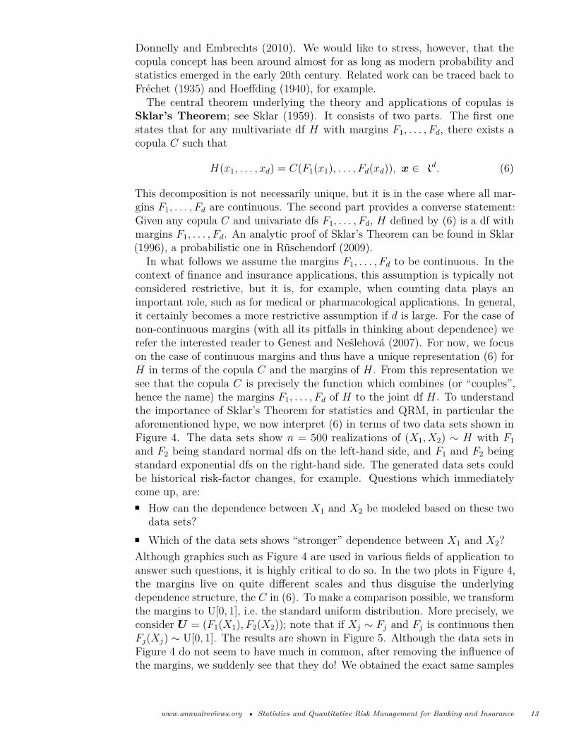
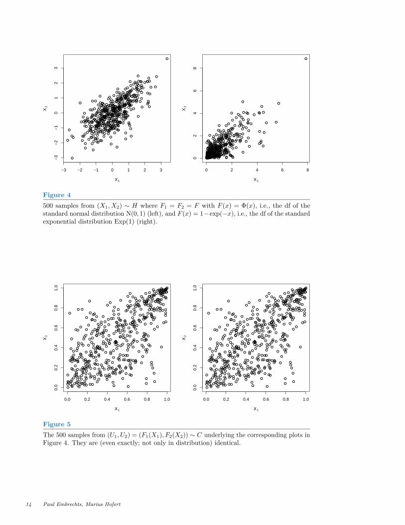
In what follows we assume the margins F1, . . . , Fd to be continuous. In thecontext of finance and insurance applications, this assumption is typically notconsidered restrictive, but it is, for example, when counting data plays animportant role, such as for medical or pharmacological applications. In general,it certainly becomes a more restrictive assumption if d is large. For the case ofnon-continuous margins (with all its pitfalls in thinking about dependence) werefer the interested reader to Genest and Nešlehová (2007). For now, we focuson the case of continuous margins and thus have a unique representation (6) forH in terms of the copula C and the margins of H. From this representation wesee that the copula C is precisely the function which combines (or “couples”,hence the name) the margins F1, . . . , Fd of H to the joint df H. To understandthe importance of Sklar’s Theorem for statistics and QRM, in particular theaforementioned hype, we now interpret (6) in terms of two data sets shown inFigure 4. The data sets show n = 500 realizations of (X1, X2) ∼ H with F1and F2 being standard normal dfs on the left-hand side, and F1 and F2 beingstandard exponential dfs on the right-hand side. The generated data sets couldbe historical risk-factor changes, for example. Questions which immediatelycome up, are:
How can the dependence between X1 and X2 be modeled based on these twodata sets?Which of the data sets shows “stronger” dependence between X1 and X2?
Although graphics such as Figure 4 are used in various fields of application toanswer such questions, it is highly critical to do so. In the two plots in Figure 4,the margins live on quite different scales and thus disguise the underlyingdependence structure, the C in (6). To make a comparison possible, we transformthe margins to U[0, 1], i.e. the standard uniform distribution. More precisely, weconsider U = (F1(X1), F2(X2)); note that if Xj ∼ Fj and Fj is continuous thenFj(Xj) ∼ U[0, 1]. The results are shown in Figure 5. Although the data sets inFigure 4 do not seem to have much in common, after removing the influence ofthe margins, we suddenly see that they do! We obtained the exact same samples
www.annualreviews.org • Statistics and Quantitative Risk Management for Banking and Insurance 13
●
●
●
●
●●
●
●
●
●
●
●
●
●
●
●
●
●
●
●
●
●
●
●
●
●
●
●
●
●
●●
●
● ●
●
●
●
●●
●
●
●
●
●
●
●
●
●
●
●
●
●
●
● ●
●●
●
●
●
●
●
●
●
●●
●
●
●
●
●
●
●
●
●
●
●
●
●
●
●
●
●
●
●
●
●
●●
●
●
●
●
●
●
●
●
●●
●
●
●
●
●
●
●
●
●●
●
●
● ●●
●
●●
●
●
●
●
●
●
●
●
●
●
●
●
●
●
●
●
●
●
●
●
●
●
●
●
●
●
●
●
●●
●
●
●●
●
●
●
●
●
●
●
●
●
●
●
●●
●
●
●
●
●
●
●●
●
●
●
●
●●
●
●
●●
●
●
●
●
●
●
●
●
●
●
●
●
●
●
●
●
●
●
●●
●●
●
●
●
●
●
●
●
●●
●
●
●
●●
●
●
●
●
●
●
●
●
●
●
●
●
●●● ●
●
●
●
●
●
●
●
●
●
●
●●
●
●
●
●
●
●
●
●
●
●
●
●
●
●
●
●
●
●
●
●
● ●
●
●
●
●
●
●
●
●
●
●
●
●●
●
●
●●
●
●
●
●
●
●
●
● ●
●
●
●
●
●
●
●
●
●●
●
●
●
●
●
●●
●
●
●
●
●
●
●
●
●
●
●
●
●
●
●
●
●
●
●
●
●●
●
●
●
●
●
●●
●
●
●
●
●
●
●
●
●●●
●●
●
●
●
●●
●
●
●●
●●
●
●●
●●
●
●●
●
●
●
●
●
●●
●
● ●
●
●
●
●
●
●
●
●
●
●
●
● ●
● ●●
●
●
●
●
●
●
●
●
●
●
●
●
●●
●
●
●
● ●
●
●
●
●
●
●●
●
●
●
●
●
●
●
●
●
●●
●
●
●
●
●
●
●
●
●
●
●
●
●
●
●
●
●
●
●
●
●
●
●
●●
●
●
●
●
●
●
●
●
●
●
●
●
●
●
●
●
●
●
●
●
●
●●
●
●
●
●
●
●
●
●
●
●
●
●
●●
●
●
−3 −2 −1 0 1 2 3
−3
−2
−1
01
23
X1
X2
●
●
●
●
●●●
●
●●
●
●
●
●
●
●
●
●
●●
●
●●
●
●
●
●
●
●●
●●
●
● ●
●
●
●● ●
●
●
●
●
●
●
●
●●
●
●
●
●
●
● ●
●●
●●
●
●
●
●
●
● ●
●
●
●
●
●●
●●
●
●
●●
●
●
●
●
●
●●
●
●
●●
●
●
●
●
●
●
●●
●
●
●
●
●●●
●
● ●
●●
●
●
● ● ●●●●
●
●
●
●
●
●
●
●
●
●
●
●
●
●
●
●
●
●
●
●
●
●
●
●
●
●●
●
●●
●
●●●
●
●●
●
●
●
●
●
●
●
●
●●
●●
●
●
●
●
●●
●●
●
●
●●
●
●
●●
●
●
●
●
●
●
●
●●
●
●
●
●
●
●
●
●
●● ●
●●
●
●
●●
●
●
●
●●
●
●
●
●●
●
●
●
●
●●
●●
●
●
●
●
●●● ●
●
●
●
●
●
●
●
●
●
●
● ●
●
●
●
●
●
●
●
●
●
●
●
●
●
●
●
●
●
●
● ●
● ●
●
●
●
●
●
●
●
●
●
●
●
●●
●
●
●●
●
●
●
●
●
●●
● ●
●
●
●
●
●
●
●
●
●●●
●●
●
●
●●
●●
●
●
●
●
●
●●●●
●
●
●
●
●
●
●
●
●
●●●●
●●
●
●●
●●
●●
●
●
●
●
●● ●●●
●
●
●
●●
●
●●●● ●
●
●●
●●
●
●●
●
●
●
●
●●●
●
● ●
●
●
●
●
●
●
●
●
●
●
●
● ●
● ●●
●
●
●
●
●
●●
●●
●
●
●
●●●
●
●● ●
●
●●
●
●●●
●●
●
●
● ●
●
●●
●●
●
●
●
●
●
●●
●
●
●
●
●
●
●
●
●
●
●
●
●
●
●
●
●●
●
●●●
●
●
●
●
●
●
●
●
●
●
●
●●
●
●
●
●
●●
●
●
●
●
●
●●
●
●
●
●
●
●●
●
●
0 2 4 6 8
02
46
8
X1X
2
Figure 4500 samples from (X1, X2) ∼ H where F1 = F2 = F with F (x) = Φ(x), i.e., the df of thestandard normal distribution N(0, 1) (left), and F (x) = 1−exp(−x), i.e., the df of the standardexponential distribution Exp(1) (right).
●
●
●
●
●●
●
●
●
●
●
●
●
●
●
●
●
●
●
●
●
●
●
●
●
●
●
●
●
●
●●
●
● ●
●
●
●
●
●
●
●
●
●
●
●
●
●
●
●
●
●
●
●
●●
●
●
●
●
●
●
●
●
●
●
●
●
●
●
●
●
●
●
●
●
●
●
●
●
●
●
●
●
●
●
●
●
●
●
●
●
●
●
●
●
●
●
●
●
●
●
●
●
●
●
●
●
●●
●
●
●●
●
●
●●
●
●
●
●
●
●
●
●
●
●
●
●
●
●
●
●
●
●
●
●
●
●
●
●
●
●
●
●
●
●
●
●
●●
●
●
●
●
●
●
●
●
●
●
●
●
●
●
●
●
●
●
●
●
●
●
●
●
●
●
●
●
●
●
●
●
●
●
●
●
●
●
●
●
●
●
●
●
●
●
●
●
●
●
●
●
●
●
●
●
●
●
●
●
●
●
●
●
●
●
●
●
●
●
●
●
●
●
●
●
●
●
●
●
●● ●
●
●
●
●
●
●
●
●
●
●
●
●
●
●
●
●
●
●
●
●
●
●
●
●
●
●
●
●
●
●
●
●
●●
●
●
●
●
●
●
●
●
●
●
●
●●
●
●
●
●
●
●
●
●
●
●
●
●●
●
●
●
●
●
●
●
●
●
●
●
●
●
●
●
●●
●
●
●
●
●
●
●
●
●
●
●
●
●
●
●
●
●
●
●
●
●
●
●
●
●
●
●
●
●
●
●
●
●
●
●
●
●
●●
●
●●
●
●
●
●
●
●
●
●●
●●
●
●
●
●
●
●
●●
●
●●
●
●
●
●
●
●●
●
●
●
●
●
●
●
●
●
●
●
●●
● ●
●
●
●
●
●
●
●
●
●
●
●
●
●
●●
●
●
●
●●
●
●
●
●
●
●●
●
●
●
●
●
●
●
●
●
●
●
●
●
●
●
●
●
●
●
●
●
●
●
●
●
●
●
●
●
●
●
●
●
●
●●
●
●
●
●
●
●
●
●
●
●
●
●
●
●
●
●
●
●
●
●
●
●
●
●
●
●
●
●
●
●
●
●
●
●
●
●
●
●
●
0.0 0.2 0.4 0.6 0.8 1.0
0.0
0.2
0.4
0.6
0.8
1.0
X1
X2
●
●
●
●
●●
●
●
●
●
●
●
●
●
●
●
●
●
●
●
●
●
●
●
●
●
●
●
●
●
●●
●
● ●
●
●
●
●
●
●
●
●
●
●
●
●
●
●
●
●
●
●
●
●●
●
●
●
●
●
●
●
●
●
●
●
●
●
●
●
●
●
●
●
●
●
●
●
●
●
●
●
●
●
●
●
●
●
●
●
●
●
●
●
●
●
●
●
●
●
●
●
●
●
●
●
●
●●
●
●
●●
●
●
●●
●
●
●
●
●
●
●
●
●
●
●
●
●
●
●
●
●
●
●
●
●
●
●
●
●
●
●
●
●
●
●
●
●●
●
●
●
●
●
●
●
●
●
●
●
●
●
●
●
●
●
●
●
●
●
●
●
●
●
●
●
●
●
●
●
●
●
●
●
●
●
●
●
●
●
●
●
●
●
●
●
●
●
●
●
●
●
●
●
●
●
●
●
●
●
●
●
●
●
●
●
●
●
●
●
●
●
●
●
●
●
●
●
●
●● ●
●
●
●
●
●
●
●
●
●
●
●
●
●
●
●
●
●
●
●
●
●
●
●
●
●
●
●
●
●
●
●
●
●●
●
●
●
●
●
●
●
●
●
●
●
●●
●
●
●
●
●
●
●
●
●
●
●
●●
●
●
●
●
●
●
●
●
●
●
●
●
●
●
●
●●
●
●
●
●
●
●
●
●
●
●
●
●
●
●
●
●
●
●
●
●
●
●
●
●
●
●
●
●
●
●
●
●
●
●
●
●
●
●●
●
●●
●
●
●
●
●
●
●
●●
●●
●
●
●
●
●
●
●●
●
●●
●
●
●
●
●
●●
●
●
●
●
●
●
●
●
●
●
●
●●
● ●
●
●
●
●
●
●
●
●
●
●
●
●
●
●●
●
●
●
●●
●
●
●
●
●
●●
●
●
●
●
●
●
●
●
●
●
●
●
●
●
●
●
●
●
●
●
●
●
●
●
●
●
●
●
●
●
●
●
●
●
●●
●
●
●
●
●
●
●
●
●
●
●
●
●
●
●
●
●
●
●
●
●
●
●
●
●
●
●
●
●
●
●
●
●
●
●
●
●
●
●
0.0 0.2 0.4 0.6 0.8 1.0
0.0
0.2
0.4
0.6
0.8
1.0
X1
X2
Figure 5The 500 samples from (U1, U2) = (F1(X1), F2(X2)) ∼ C underlying the corresponding plots inFigure 4. They are (even exactly; not only in distribution) identical.
14 Paul Embrechts, Marius Hofert
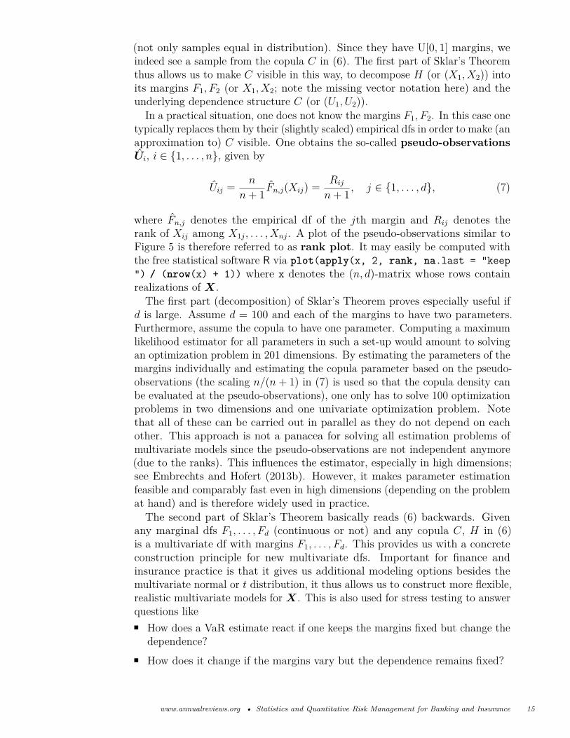
(not only samples equal in distribution). Since they have U[0, 1] margins, weindeed see a sample from the copula C in (6). The first part of Sklar’s Theoremthus allows us to make C visible in this way, to decompose H (or (X1, X2)) intoits margins F1, F2 (or X1, X2; note the missing vector notation here) and theunderlying dependence structure C (or (U1, U2)).
In a practical situation, one does not know the margins F1, F2. In this case onetypically replaces them by their (slightly scaled) empirical dfs in order to make (anapproximation to) C visible. One obtains the so-called pseudo-observationsUi, i ∈ {1, . . . , n}, given by
Uij = n
n+ 1 Fn,j(Xij) = Rij
n+ 1 , j ∈ {1, . . . , d}, (7)
where Fn,j denotes the empirical df of the jth margin and Rij denotes therank of Xij among X1j, . . . , Xnj. A plot of the pseudo-observations similar toFigure 5 is therefore referred to as rank plot. It may easily be computed withthe free statistical software R via plot(apply(x, 2, rank, na.last = "keep") / (nrow(x) + 1)) where x denotes the (n, d)-matrix whose rows containrealizations of X.The first part (decomposition) of Sklar’s Theorem proves especially useful if
d is large. Assume d = 100 and each of the margins to have two parameters.Furthermore, assume the copula to have one parameter. Computing a maximumlikelihood estimator for all parameters in such a set-up would amount to solvingan optimization problem in 201 dimensions. By estimating the parameters of themargins individually and estimating the copula parameter based on the pseudo-observations (the scaling n/(n+ 1) in (7) is used so that the copula density canbe evaluated at the pseudo-observations), one only has to solve 100 optimizationproblems in two dimensions and one univariate optimization problem. Notethat all of these can be carried out in parallel as they do not depend on eachother. This approach is not a panacea for solving all estimation problems ofmultivariate models since the pseudo-observations are not independent anymore(due to the ranks). This influences the estimator, especially in high dimensions;see Embrechts and Hofert (2013b). However, it makes parameter estimationfeasible and comparably fast even in high dimensions (depending on the problemat hand) and is therefore widely used in practice.The second part of Sklar’s Theorem basically reads (6) backwards. Given
any marginal dfs F1, . . . , Fd (continuous or not) and any copula C, H in (6)is a multivariate df with margins F1, . . . , Fd. This provides us with a concreteconstruction principle for new multivariate dfs. Important for finance andinsurance practice is that it gives us additional modeling options besides themultivariate normal or t distribution, it thus allows us to construct more flexible,realistic multivariate models for X. This is also used for stress testing to answerquestions like
How does a VaR estimate react if one keeps the margins fixed but change thedependence?How does it change if the margins vary but the dependence remains fixed?
www.annualreviews.org • Statistics and Quantitative Risk Management for Banking and Insurance 15
Another important aspect of the second part of Sklar’s Theorem is that it givesus a sampling algorithm for dfs H constructed from copula models. This isheavily used in practice as realistic models are rarely analytically tractable andthus are often evaluated based on simulations. The algorithm implied by thesecond part of Sklar’s Theorem for sampling X ∼ H where H is constructedfrom a copula C and univariate dfs F1, . . . , Fd is as follows:Algorithm 3.11) Sample U ∼ C;2) Return X = (X1, . . . , Xd) where Xj = F←j (Uj), j ∈ {1, . . . , d}.It should by now be clear to the reader how we constructed Figures 4 and
5. In line with Algorithm 3.1, we first constructed a sample of size 500 fromU ∼ C for C being a Gumbel copula (with parameter such that Kendall’s tauequals 0.5). This is shown in Figure 5. We then used the quantile function of thestandard normal distribution to map U to X having N(0, 1) margins (shownon the left-hand side of Figure 4) and similarly for the standard exponentialmargins on the right-hand side of Figure 4.After this brief introduction to the modeling of stochastic dependence with
copulas, a few remarks are in order. Summaries of the main results partlyincluding historical overviews can be found in the textbooks of Schweizer andSklar (1983, Chapter 6), Nelsen (1999), Cherubini et al. (2004), or Jaworski et al.(2010). The relevance for finance is summarized in Embrechts (2009). AddingSchweizer (1991), both papers together give an idea of the key developments.Embrechts (2009) also recalls some of the early discussions between protagonistsand antagonists of the usefulness of copulas in insurance and finance in generaland QRM in particular.
History has moved on and by now copula technology forms a well-establishedtool set for QRM. Like VaR, also the copula concept is marred with warningsand restrictions when it comes to its applications. An early telling example is theuse of the Gaussian copula (the copula C corresponding to H being multivariatenormal via (6)) in the realm of CDO-pricing, an application which for somelay at the core of the subprime crisis; see for instance the online publication(blog) Salmon (2009). Somewhat surprisingly, the statistical community boughtthe arguments; see Salmon (2012). This despite the fact that the weakness(even impossibility) of the Gaussian copula for modeling joint extremes wasknown for almost 50 years: Sibuya (1959) showed that the Gaussian copuladoes not exhibit a notion referred to as tail dependence; see McNeil et al. (2005,Section 5.2.3). Informally, the latter notion describes the probability that one(of two) rvs takes on a large (small) value, given that the other one takes on alarge (small) value; in contrast to the Gaussian copula, a Gumbel copula (beingpart of the Archimedean class) is able to capture (upper) tail dependence andwe may already suspect that by looking at Figure 5. With the notion of taildependence at hand, it is not difficult to see its importance for CDO pricingmodels (or more generally, intensity-based default models) such as the one basedon Gaussian copulas (see Li (2000)), Archimedean copulas (see Schönbucherand Schubert (2001)), or nested Archimedean copulas (see Hofert and Scherer
16 Paul Embrechts, Marius Hofert
(2011)); the latter two references introduce models which are able to capture taildependence. Due to its importance for QRM, Sibuya (1959) and, more broadly,tail dependence was referred to in the original Embrechts et al. (2002, Section 4.4).We repeat the main message from the latter paper: copulas are a very usefulconcept for better understanding the concept of stochastic dependence, not apanacea for its modeling. The title of Lipton and Rennie (2007) is telling in thiscontext; see also the discussions initiated by Mikosch (2006).As mentioned before, within QRM, copulas have numerous applications to-
wards risk aggregation and stress testing, and as such have entered the regulatoryguidelines. Below we briefly address some of the current challenges; they aremainly related to high-dimensionality, statistical estimation, and numericalcalculations.
A large part of research on copulas is conducted and presented in the bivariatecase (d = 2). Bivariate copulas are typically convenient to work with, the cased = 2 offers more possibilities to construct copulas (via geometric approaches),required quantities can often be derived by hand, graphics (of the df or, if itexists, its density) can still be drawn without losing information, and numericalissues are often not severe or negligibly small. The situation is different for d > 2and fundamentally different for d� 2 (even if we stay far below d = 1000). Ingeneral, the larger the dimension d, the more complicated it is to come up witha numerically tractable model which is flexible enough to account for real databehavior. Joe (1997, pp. 84) presents several desirable properties of multivariatedistributions. However, to date, no model is known which exhibits all suchproperties.The t copula belongs to the most widely used copula models; see Demarta
and McNeil (2005) for an introduction and possible extensions. Besides anexplicit density, it admits tail dependence and can be sampled comparably fast;it also incorporates the Gaussian copula as limiting case, which, despite all itslimitations, is still a popular model. This makes the t copula especially attractivefor practical applications even in large dimensions. From a more technical pointof view, a d-dimensional t copula with ν > 0 degrees of freedom and correlationmatrix P can be written as
C(u) = tν,P (t−1ν (u1), . . . , t−1
ν (ud)), u ∈ [0, 1]d,
where tν,P denotes the df of a multivariate t distribution with ν degrees offreedom and correlation matrix P (corresponding to the dispersion matrix Σ interms of which the multivariate t distribution is defined in general; see Demartaand McNeil (2005)) and t−1
ν denotes the quantile function of a univariate tdistribution with ν degrees of freedom. From this formula we already see thatthe components involved in evaluating a t copula are non-trivial. Neither tν,Pnor t−1
ν are known explicitly. Especially the former is a problem and for d > 3,randomized quasi Monte Carlo methods are used (in the well-known R packagemvtnorm) to evaluate the d-dimensional integral; see Genz and Bretz (2009,Section 5.5.1). Furthermore, the algorithm requires ν to be an integer, which isa limitation for which no easy solution is available yet.The Gaussian and t copula families belong to the class of elliptical copulas
www.annualreviews.org • Statistics and Quantitative Risk Management for Banking and Insurance 17
and are given implicitly by solving (6) for C in the case where H is the df ofan elliptical distribution. A different ansatz stems from Archimedean copulas,which are given explicitly in terms of a so-called generator ψ : [0,∞)→ [0, 1]via
C(u) = ψ(ψ−1(u1) + · · ·+ ψ−1(ud)), u ∈ [0, 1]d; (8)
see McNeil and Nešlehová (2009). For the Gumbel copula family, ψ(t) =exp(−t1/θ), θ ≥ 1. Archimedean copulas allow for a fast sampling algorithm,see Marshall and Olkin (1988), and, in contrast to elliptical copulas, are notlimited to radial symmetry. Elliptical copulas put the same probability massin the upper-right corner than in the lower-left corner of the distribution andthus value joint large gains in the same way as joint large losses. On the otherhand, it directly follows from (8) that Archimedean copulas are symmetric, thatis, invariant under permutation of the arguments. This is also visible from thesymmetry with respect to the diagonal in Figure 5. Still, the flexibility in the(upper or lower) tail of copulas such as the Gumbel are interesting for practicalapplications and Archimedean copula families such as the Clayton or Gumbelbelong to the most widely used copula models (the Gumbel family additionallybelongs to the class of extreme value copulas and is one of the rare comparablytractable examples in this class).
The rather innocent functional form (8) bears interesting numerical problems,already in small to moderate dimensions which have even led to wrong statementsin the more recent literature. The copula density is easily seen to be
c(u) = (−1)dψ(d)(ψ−1(u1) + · · ·+ ψ−1(ud))d∏j=1
(−ψ−1)′(uj), u ∈ (0, 1)d.
In particular, it involves the dth generator derivative. For d large, these aredifficult to access. For the Gumbel copula, an explicit form for (−1)dψ(d) hasonly recently been found; see Hofert et al. (2012). The formula is
(−1)dψ(d)(t) = ψ(t)td
d∑k=1
adk(α)tαk,
adk(α) = (−1)d−kd∑j=k
αjs(d, j)S(j, k) = d!k!
k∑j=1
(k
j
)(αj
d
)(−1)d−j,
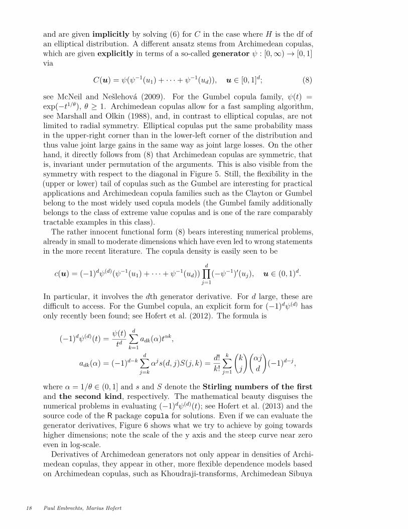
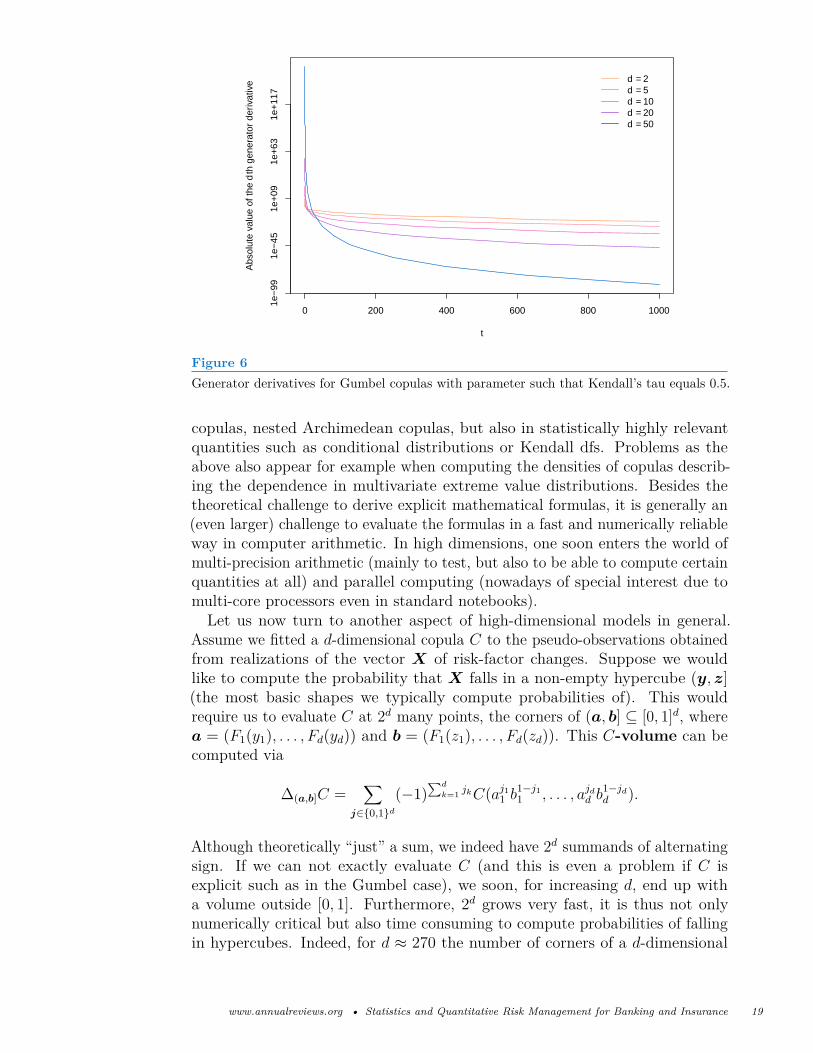
where α = 1/θ ∈ (0, 1] and s and S denote the Stirling numbers of the firstand the second kind, respectively. The mathematical beauty disguises thenumerical problems in evaluating (−1)dψ(d)(t); see Hofert et al. (2013) and thesource code of the R package copula for solutions. Even if we can evaluate thegenerator derivatives, Figure 6 shows what we try to achieve by going towardshigher dimensions; note the scale of the y axis and the steep curve near zeroeven in log-scale.Derivatives of Archimedean generators not only appear in densities of Archi-
medean copulas, they appear in other, more flexible dependence models basedon Archimedean copulas, such as Khoudraji-transforms, Archimedean Sibuya
18 Paul Embrechts, Marius Hofert
0 200 400 600 800 1000
1e−
991e
−45
1e+
091e
+63
1e+
117
t
Abs
olut
e va
lue
of th
e d
th g
ener
ator
der
ivat
ive d = 2
d = 5d = 10d = 20d = 50
Figure 6Generator derivatives for Gumbel copulas with parameter such that Kendall’s tau equals 0.5.
copulas, nested Archimedean copulas, but also in statistically highly relevantquantities such as conditional distributions or Kendall dfs. Problems as theabove also appear for example when computing the densities of copulas describ-ing the dependence in multivariate extreme value distributions. Besides thetheoretical challenge to derive explicit mathematical formulas, it is generally an(even larger) challenge to evaluate the formulas in a fast and numerically reliableway in computer arithmetic. In high dimensions, one soon enters the world ofmulti-precision arithmetic (mainly to test, but also to be able to compute certainquantities at all) and parallel computing (nowadays of special interest due tomulti-core processors even in standard notebooks).Let us now turn to another aspect of high-dimensional models in general.
Assume we fitted a d-dimensional copula C to the pseudo-observations obtainedfrom realizations of the vector X of risk-factor changes. Suppose we wouldlike to compute the probability that X falls in a non-empty hypercube (y, z](the most basic shapes we typically compute probabilities of). This wouldrequire us to evaluate C at 2d many points, the corners of (a, b] ⊆ [0, 1]d, wherea = (F1(y1), . . . , Fd(yd)) and b = (F1(z1), . . . , Fd(zd)). This C-volume can becomputed via
∆(a,b]C =∑
j∈{0,1}d
(−1)∑d
k=1 jkC(aj11 b1−j11 , . . . , ajdd b
1−jdd ).
Although theoretically “just” a sum, we indeed have 2d summands of alternatingsign. If we can not exactly evaluate C (and this is even a problem if C isexplicit such as in the Gumbel case), we soon, for increasing d, end up witha volume outside [0, 1]. Furthermore, 2d grows very fast, it is thus not onlynumerically critical but also time consuming to compute probabilities of fallingin hypercubes. Indeed, for d ≈ 270 the number of corners of a d-dimensional
www.annualreviews.org • Statistics and Quantitative Risk Management for Banking and Insurance 19
hypercube is roughly equal to the number of atoms in the universe. Clearly,for d = 1000 approximation schemes and possibly new approaches must bedeveloped.New high-dimensional dependence models for X that recently became of
interest are hierarchical models. Through a matrix of parameters, ellipticalcopulas such as the Gaussian or t copulas allow for
(d2
)-many (an additional
one for the t copula) parameters. Symmetric models such as (8) typically allowfor just a handful of parameters, depending on the parametric generator underconsideration. Hierarchical models try to go somewhere in-between, which isoften a good strategy for d large. While estimating
(d2
)-many parameters may be
time-consuming and, for example in the case of a small sample size, not justifiableby the data at hand or task in mind, using the assumption of symmetry for blocksor groups of variables among X allows to reduce the number of parameters tofall in between a fully symmetric model and a model considering parameters forall
(d2
)pairs of variables. Extending (8) to allow for hierarchies can be achieved
in various ways, see for example McNeil (2008) or Hofert (2012). Reducingthe parameters in elliptical models can be done by considering block matrices;see Torrent-Gironella and Fortiana (2011) which is one of the rare publicationscarefully considering numerical issues behind the scenes as well. For a differentidea to incorporate groups in t copulas, see Demarta and McNeil (2005).
SUMMARY POINTSOverall, to our experience, there are many challenges in the area of highdimensional dependence modeling. It does not seem to be a pleasingtask to go there as numerics will heavily enter soon after one leaves the“comfort zone” of d being as small as two or three. However, from apractical point of view it is necessary. Working in high dimensions mayrequire starting from scratch, model building already has to take numericsinto account, not only mathematical beauty or convenience. The sameapplies to the (even more complicated) case of time dependent models notdiscussed here. To give an example, sampling dependent Lévy processeswith the notion of Lévy copulas to model dependence between jumps istypically also numerically a non-trivial task and limited to rather smalldimensions. Although mathematically d is just a natural number and canbe increased arbitrarily in the above discussion and formulas, solutionsto the problems mentioned above heavily depend on d. In the end of the(bank’s) day, models, estimators, stress tests etc. have to be computed andthus, additionally, require reliable software behind the scenes. It is to beencouraged that academia contributes here as well (and gets scientificallyrewarded for entering this time-consuming process), as new statistical modelsand procedures (including their limitations) are typically best understoodby those who invented them. Being pressed for time in business practiceoften requires to implement a model in a small amount of time, basicallyuntil it “works”. However, proper testing of statistical software has to gofar beyond this point and extensive test suites have to be put in place.
20 Paul Embrechts, Marius Hofert

Open source statistical software (slowly finding its way into business practicebut still not used to a sufficient degree) typically guarantees more stable andreliable procedures as anyone can report bugs, for example. Furthermore,open source increases the understanding of new models and the recognitionof their limitations. Software development also has to be communicatedon an academic level as it is already part of (but also limited to) statisticscourses. Preparing students for (or at least to be aware of) the computationalchallenges they will meet in practice should rather become the rule thanthe exception.
4. Risk aggregation and model uncertaintyThe subadditivity property of a risk measure is often defended in order toachieve a coherent, consistent way to aggregate risks across different entities(business lines, say) and also in order to find methodologically consistent ways todisaggregate, also referred to risk allocation. Further, in the background lies theconcept of risk diversification. In this section we will give a very brief overviewof some of the underlying mathematical issues. Given a general risk measure R(examples treated so far include R = VaR, R = ES), for d risks X1, . . . , Xd, wedefine the coefficient of diversification as
DR(X) =R(∑d
j=1Xj)∑dj=1R(Xj)
.
In the superadditive case, DR(X) may be larger than 1; an important question is“by how much?”, and this in particular as a function of the various probabilisticassumptions on the joint df H of X. Model Uncertainty in particular enters if weonly have partial information on the marginal dfs F1, . . . , Fd and a/the copula C;see our discussion in the previous section. The mathematical problem underlyingthe calculation of DR(X) has a long history. Below we will content ourselveswith a very brief summary pointing the reader to some of the basic literature;we will also present some examples aimed at understanding the range of valuesfor DR(X) if only information on F1, . . . , Fd is available (the unconstrainedproblem).The reference on the topic, from a more mathematical point of view is
Rüschendorf (2013). As can be seen from the title, it contains all relevant topicsto be addressed in this section. It also contains an extensive list of historicallyrelevant references. We know that in the case of R = VaR, DR(X) > 1 typicallyhappens for the Fj’s being very heavy tailed (e.g. independent and infinitemean), very skew (see Example 2.3) or for the risks X1, . . . , Xd exhibiting aspecial dependence structure (even with F1 = · · · = Fd being N(0, 1)); McNeilet al. (2005, Example 6.22). Interesting questions for practice now are: (Q1)Given a specific model leading to superadditivity of DR(X), by how much canDR(X) > 1, and (Q2) which dependence structures between X1, . . . , Xd leadto such extreme cases. Are these realistic from a practical point of view? And
www.annualreviews.org • Statistics and Quantitative Risk Management for Banking and Insurance 21
finally, (Q3) under what kind of dependence information between X1, . . . , Xd
can such bounds be computed. Besides the above textbook reference, questions(Q1)–(Q3) are discussed in detail in Embrechts et al. (2013). From the latterpaper we borrow the example below.
Example 4.1Suppose Xj ∼ Pareto(2), j ∈ {1, . . . , d}, i.e. 1−Fj(x) = P(Xj > x) = (1 +x)−2,x ≥ 0. For d = 8 and α = 0.99, VaRα(Xj) = 9 resulting in ∑8
j=1 VaRα(Xj) = 72,the so-called comonotonic case for C; see McNeil et al. (2005, Proposition 6.15).An exact upper bound on DR(X) can be given in this case, it equals about 2;see Table 4 in Embrechts et al. (2013). The latter paper also contains lightertailed examples like log-normal and gamma; see Figure 4 in the latter paper.Here the upper bound for DR(X) for α = 0.99 is between 1.15 and 1.5. Themain lesson learned is that DR(X) can be considerably larger than 1 in theunconstrained case. Constraining the rvs to e.g. positive quadrant dependencedoes not change the bounds by much. For X being elliptically distributed, orfor R = ES, the upper bound is always 1! Note that for DR(X) > 1, we enterthe world of non-coherence, i.e., the risk of the overall portfolio position ∑d
j=1Xj
is not covered, in a possibly conservative way, by the sum of the marginalrisk contributions. In finance parlance, people would say that in such a case,“diversification does not work”.
For the above kind of problems, techniques from the realm of OperationsResearch will no doubt turn out to be relevant. Key tools to look for are Robustand Convex Optimization; see for instance Ben-Tal et al. (2009) and Boydand Vandenberghe (2004). Early work, stressing the link between OperationsResearch and QRM, especially in the context of the calculation of ES is by StanUryasev and R. Tyrell Rockafellar; see for instance Uryasev and Rockafellar(2013) and Chun et al. (2012).
SUMMARY POINTSIn this final section, we only briefly entered into the field of Model Uncer-tainty. Going forward, and in the wake of the recent financial crisis, thisarea of research will gain importance. Other areas of promising research,which for reasons of space limitations we were not able to discuss, are HighFrequency (Inter Day) Data in finance, and Systemic Risk (Network Theory).For the former, the classic “that started it all” is Dacorogna et al. (2001).By now, the field is huge! A more recent edited volume is Viens et al. (2012).For a start on some of the more mathematical work on Systemic Risk andNetwork Theory, we suggest interested readers to start with papers on thetopic by Rama Cont (Imperial College, London) and Tom Hund (McMasterUniversity, Hamilton, Canada).
22 Paul Embrechts, Marius Hofert

AcknowledgementsWe apologize in advance to all the investigators whose research could not beappropriately cited owing to space limitations.
www.annualreviews.org • Statistics and Quantitative Risk Management for Banking and Insurance 23
ReferencesAlbanese, C (1997), Credit exposure, diversification risk and coherent VaR,preprint, Department of Mathematics, University of Toronto.
Andersen, TG, Bollerslev, T, Christoffersen, PF, and Diebold, Fx (2013), Fi-nancial risk measurement for financial risk management, Handbook of theEconomics of Finance, ed. by G Constantinides, M Harris, and R Stulz,vol. 2, Amsterdam: Elsevier Science B. V., 1127–1220.
Artzner, P, Delbaen, F, Eber, JM, and Heath, D (1999), Coherent measures ofrisk, Mathematical Finance, 9, 203–228.
Balo, Y, Lee, TH, and Saltoğlu, B (2006), Evaluating predictive performanceof Value-at-Risk models in emerging markets: a reality check, Journal ofForecasting, 25, 101–128.
Ben-Tal, A, El Ghaoui, L, and Nemirovski, A (2009), Robust Optimization,Princeton University Press.
Berkowitz, J and O’Brien, J (2002), How accurate are Value-at-Risk models atcommercial banks? Journal of Finance, 57, 1093–1111.
BIS (2012), Fundamental review of the trading book, http://www.bis.org/publ/bcbs219.pdf (2012-02-03).
Boyd, S and Vandenberghe, L (2004), Convex Optimization, Princeton UniversityPress.
Chavez-Demoulin, V and McGill, JA (2012), High-frequency financial datamodeling using Hawkes processes, Journal of Banking and Finance, 36(12),3415–3426.
Chavez-Demoulin, V, Davison, AC, and McNeil, AJ (2005), Estimating value-at-risk: a point process approach, Quantitative Finance, 5(2), 227–234.
Chavez-Demoulin, V, Embrechts, P, and Sardy, S (2013a), Extreme-quantiletracking for financial time series, Journal of Econometrics, to appear.
Chavez-Demoulin, V, Embrechts, P, and Hofert, M (2013b), An extreme valueapproach for modeling operational risk losses depending on covariates.
Cherubini, U, Luciano, E, and Vecchiato, W (2004), Copula Methods in Finance,Wiley.
Christian Gourieroux, JJ (2001), Financial Econometrics: Problems, Models andMethods, Princeton: Princeton University Press.
Chun, SY, Shipiro, A, and Uryasev, S (2012), Conditional Value-at-Risk andAverage Value-at-Risk: Estimation and Asymptotics, Operations Research,60(4), 739–756.
Cont, R, Deguest, R, and Scandolo, G (2010), Robustness and sensitivity analysisof risk measurement procedures, Quantitative Finance, 10(6), 593–606.
Dacorogna, MM, Gençay, R, Müller, U, Olsen, RB, and Pictet, OV (2001), AnIntroduction to High-Frequency Finance, Academic Press.
Daníelsson, J (2011), Financial Risk Forecasting, Chichester: Wiley.Das, B, Embrechts, P, and Fasen, V (2013), Four Theorems and a FinancialCrisis, International Journal of Approximate Reasoning, to appear,http://www.math.ethz.ch/~embrechts/ftp/Four_Theorems_2012.pdf(2013-02-03).
24 Paul Embrechts, Marius Hofert
Delbaen, F (2012), Monetary Utility Functions, Osaka University Press.Dell’Aquila, R and Embrechts, P (2006), Extremes and robustness: a contradic-tion? Financial Markets and Portfolio Management, 20, 103–118.
Demarta, S and McNeil, AJ (2005), The t Copula and Related Copulas, Inter-national Statistical Review, 73(1), 111–129.
Diebold, FX, Doherty, NA, and J., HR (2010), The Known, the Unknown, andthe Unknowable in Financial Risk Management: Measurement and TheoryAdvancing Practice, Princeton University Press.
Donnelly, C and Embrechts, P (2010), The devil is in the tails: actuarial mathe-matics and the subprime mortgage crisis, ASTIN Bulletin, 40(1), 1–33.
Embrechts, P (2009), Copulas: A personal view, Journal of Risk and Insur-ance, 76, 639–650.
Embrechts, P, McNeil, AJ, and Straumann, D (1999), Correlation: Pitfallsand Alternatives, RISK Magazine, 69–71, http://www.math.ethz.ch/~mcneil/ftp/risk.pdf (2013-02-16).
Embrechts, P, McNeil, AJ, and Straumann, D (2002), Correlation and Depen-dency in Risk Management: Properties and Pitfalls, Risk Management:Value at Risk and Beyond, ed. by M Dempster, Cambridge UniversityPress, 176–223.
Embrechts, P, Puccetti, G, and Rüschendorf, L (2013), Model uncertainty andVaR aggregation, Journal of Banking and Finance, 37(8), 2750–2764.
Embrechts, P and Hofert, M (2013a), A note on generalized inverses, Math-ematical Methods of Operations Research, doi:http://dx.doi.org/10.1007/s00186-013-0436-7.
Embrechts, P and Hofert, M (2013b), Statistical inference for copulas in highdimensions: A simulation study, ASTIN Bulletin, 43(2), 81–95, doi:http://dx.doi.org/10.1017/asb.2013.6.
Embrechts, P, Kaufmann, R, and Patie, P (2005), Strategic long-term financialrisks: single risk factors,Computational Optimization and Applications,32(1–2), 61–90.
Engle, R (2009), Anticipating Correlations: A New Paradigm for Risk Manage-ment, Princeton University Press.
Fishburn, PC (1984), Foundations of Risk Measurement. I. Management Sci-ence, 30, 396–406.
Föllmer, H and Schied, A (2011), Stochastic Finance: An Introduction in DiscreteTime, 3rd ed., de Gruyter.
Fréchet, M (1935), Généralisations du théorème des probabilités totales, Fun-damenta Mathematica, 25, 379–387.
Gale, D and Shapley, LS (1962), College admissions and stability of marriage,The American Mathematical Monthly, 69(1), 9–15.
Genest, C and Nešlehová, J (2007), A primer on copulas for count data, TheAstin Bulletin, 37, 475–515.
Genest, C, Gendron, M, and Bourdeau-Brien, M (2009), The Advent of Copulasin Finance, The European Journal of Finance, 15, 609–618.
Genton, MG (2004), Skew-Elliptic Distributions and Their Applications: AJourney Beyond Normality, Boca Raton: Chapman & Hall/CRC.
www.annualreviews.org • Statistics and Quantitative Risk Management for Banking and Insurance 25
Genz, A and Bretz, F (2009), Computation of Multivariate Normal and tProbabilities, Springer.
Giacomini, R and Komunjer, I (2005), Evaluation and combination of conditionalquantile forecasts, Journal of Business & Economic Statistics, 23, 416–431.
Gilboa, I and Schmeidler, D (1989), Maximum expected utility with a non-uniqueprior, Journal of Mathematical Economics, 18, 141–153.
Gneiting, T (2011), Making and evaluating point forecasts, Journal of theAmerical Statistical Association, 106, 746–762.
Hampel, FR, Ronchetti, EM, Rousseeuw, PJ, and Stahel, WA (2005), RobustStatistics: The Approach Based on Influence Functions, Wiley-Interscience.
Hoeffding, W (1940), Massstabinvariante Korrelationstheorie, Schriften desmathematischen Seminars und des Instituts für Angewandte Math-ematik der Universität Berlin, 5, 181–233.
Hofert, M (2012), A stochastic representation and sampling algorithm for nestedArchimedean copulas, Journal of Statistical Computation and Simula-tion, 82(9), 1239–1255, doi:http://dx.doi.org/10.1080/00949655.2011.574632.
Hofert, M and Scherer, M (2011), CDO pricing with nested Archimedean copulas,Quantitative Finance, 11(5), 775–787, doi:http://dx.doi.org/10.1080/14697680903508479.
Hofert, M, Mächler, M, and McNeil, AJ (2012), Likelihood inference for Ar-chimedean copulas in high dimensions under known margins, Journal ofMultivariate Analysis, 110, 133–150, doi:http://dx.doi.org/10.1016/j.jmva.2012.02.019.
Hofert, M, Mächler, M, and McNeil, AJ (2013), Archimedean Copulas in HighDimensions: Estimators and Numerical Challenges Motivated by FinancialApplications, Journal de la Société Française de Statistique.
Huber, PJ (1981), Robust Statistics, Wiley.Huber, PJ and Ronchetti, EM (2009), Robust Statistics, 2nd ed., Wiley.Jaworski, P, Durante, F, Härdle, WK, and Rychlik, T, eds. (2010), CopulaTheory and Its Applications, vol. 198, Lecture Notes in Statistics – Proceedings,Springer.
Joe, H (1997), Multivariate Models and Dependence Concepts, Chapman &Hall/CRC.
Jorion, P (2007), Value at Risk: The New Benchmark for Managing FinancialRisk, 3rd ed., New York: McGraw-Hill.
Kaufmann, R (2004), Long-Term Risk Management, no. 15595, PhD thesis,Department of Mathematics, ETH Zurich.
Knight, FH (1921), Risk, Uncertainty and Profit, Houghton Mifflin Co.Li, DX (2000), On Default Correlation: A Copula Function Approach, TheJournal of Fixed Income, 9(4), 43–54.
Lipton, A and Rennie, A (2007), Credit Correlation: Life After Copulas, WorldScientific Publishing Company.
Mancini, L and Trojani, F (2011), Robust Value-at-Risk prediction, Journal ofFinancial Econometrics, 9, 281–313.
26 Paul Embrechts, Marius Hofert
Marshall, AW and Olkin, I (1988), Families of Multivariate Distributions, Jour-nal of the American Statistical Association, 83(403), 834–841.
McNeil, AJ (2008), Sampling nested Archimedean copulas, Journal of Statis-tical Computation and Simulation, 78(6), 567–581.
McNeil, AJ and Frey, R (2000), Estimation of tail-related risk measures forheteroscedastic financial time series: an extreme value approach, Journal ofEmpirical Finance, 7, 271–300.
McNeil, AJ and Nešlehová, J (2009), Multivariate Archimedean copulas, d-monotone functions and l1-norm symmetric distributions, The Annals ofStatistics, 37(5b), 3059–3097.
McNeil, AJ, Frey, R, and Embrechts, P (2005), Quantitative Risk Management:Concepts, Techniques, Tools, Princeton University Press.
Mikosch, T (2006), Copulas: Tales and facts, Extremes, 9(1), 3–20.Nelsen, RB (1999), An Introduction to Copulas, Springer.Rémillard, B (2013), Statistical Methods For Financial Engineering, Chapman& Hall/CRC.
Roth, A and Shapley, L (2012), Game, set and match, http://www.economist.com/news/finance-and-economics/21564836-alvin-roth-and-lloyd-shapley-have-won-year%E2%80%99s-nobel-economics (2013-01-16).
Rüschendorf, L (2009), On the distributional transform, Sklar’s Theorem, and theempirical copula process, Journal of Statistical Planning and Inference,139(11), 3921–3927.
Rüschendorf, L (2013), Mathematical Risk Analysis: Dependence, Risk Bounds,Optimal Allocations and Portfolios, Springer.
Salmon, F (2009), Recipe for Disaster: The Formula That Killed Wall Street,http : / / www . wired . com / techbiz / it / magazine / 17 - 03 / wp _ quant ?currentPage=all (2013-02-16).
Salmon, F (2012), The formula that killed Wall Street, Significance, 9(1),16–20.
Sandström, A (2006), Solvency: Models, Assessment and Regulation, Boca Raton:Chapman & Hall/CRC.
Schönbucher, PJ and Schubert, D (2001), Copula-Dependent Default Risk inIntensity Models, http://papers.ssrn.com/sol3/papers.cfm?abstract_id=301968 (2009-12-30).
Schweizer, B (1991), Thirty years of copulas, Advances in Probability Dis-tributions with Given Marginals, ed. by G Dall’Aglio, S Kotz, and GSalinetti, Kluwer Academic Publishers, 13–50.
Schweizer, B and Sklar, A (1983), Probabilistic Metric Spaces, New York: North-Holland.
SCOR (2008), From Principle-Based Risk Management to Solvency Requirements,http : / / www . scor . com / images / stories / pdf / scorpapers / sstbook _second_edition_final.pdf (2013-02-16).
Sibuya, M (1959), Bivariate extreme statistics, I, Annals of the Institute ofStatistical Mathematics, 11(2), 195–210.
www.annualreviews.org • Statistics and Quantitative Risk Management for Banking and Insurance 27
Sklar, A (1959), Fonctions de répartition à n dimensions et leurs marges, Publi-cations de L’Institut de Statistique de L’Université de Paris, 8, 229–231.
Sklar, A (1996), Random variables, distribution functions, and copulas – apersonal look backward and forward, Distributions with Fixed Marginalsand Related Topics, 28, 1–14.
Tarullo, DK (2008), Banking on Basel: The Future of International FinancialRegulation, Washington, D. C.: Peterson Institute for International Economics.
Torrent-Gironella, G and Fortiana, J (2011), Simulation of High-Dimensionalt-Student Copulas with a Given Block Correlation Matrix, ASTIN ColloquiumMadrid 2011.
Uryasev, S and Rockafellar, RT (2013), The fundamental risk quadrangle in riskmanagement, optimization and statistical estimation, Surveys in OperationsResearch and Management Science. 18.
Viens, FG, Mariani, MC, and Florescu, I (2012), Handbook of Modeling High-Frequency Data in Finance, Wiley.
Wiener, N (1923), On the nature of mathematical thinking, AustralasianJournal of Psychology and Philosophy, 1(4), 268–272.
Wong, MCY (2013), Buble Value at Risk: A Countercyclical Risk ManagementApproach, revised edition, Wiley.
Ziegel, J (2013), Coherence and elicitability, preprint, University of Bern.
28 Paul Embrechts, Marius Hofert