Jon Clayden <j.clayden@ucl.ac.uk>

Photo by José Martín Ramírez Carrasco https://www.behance.net/martini_rc

Statistics and Imaging

DIBS Teaching Seminar, 11 Nov 2015

“Statistics is a subject that many medics find easy, but most statisticians find difficult”

— Stephen Senn (attrib.)

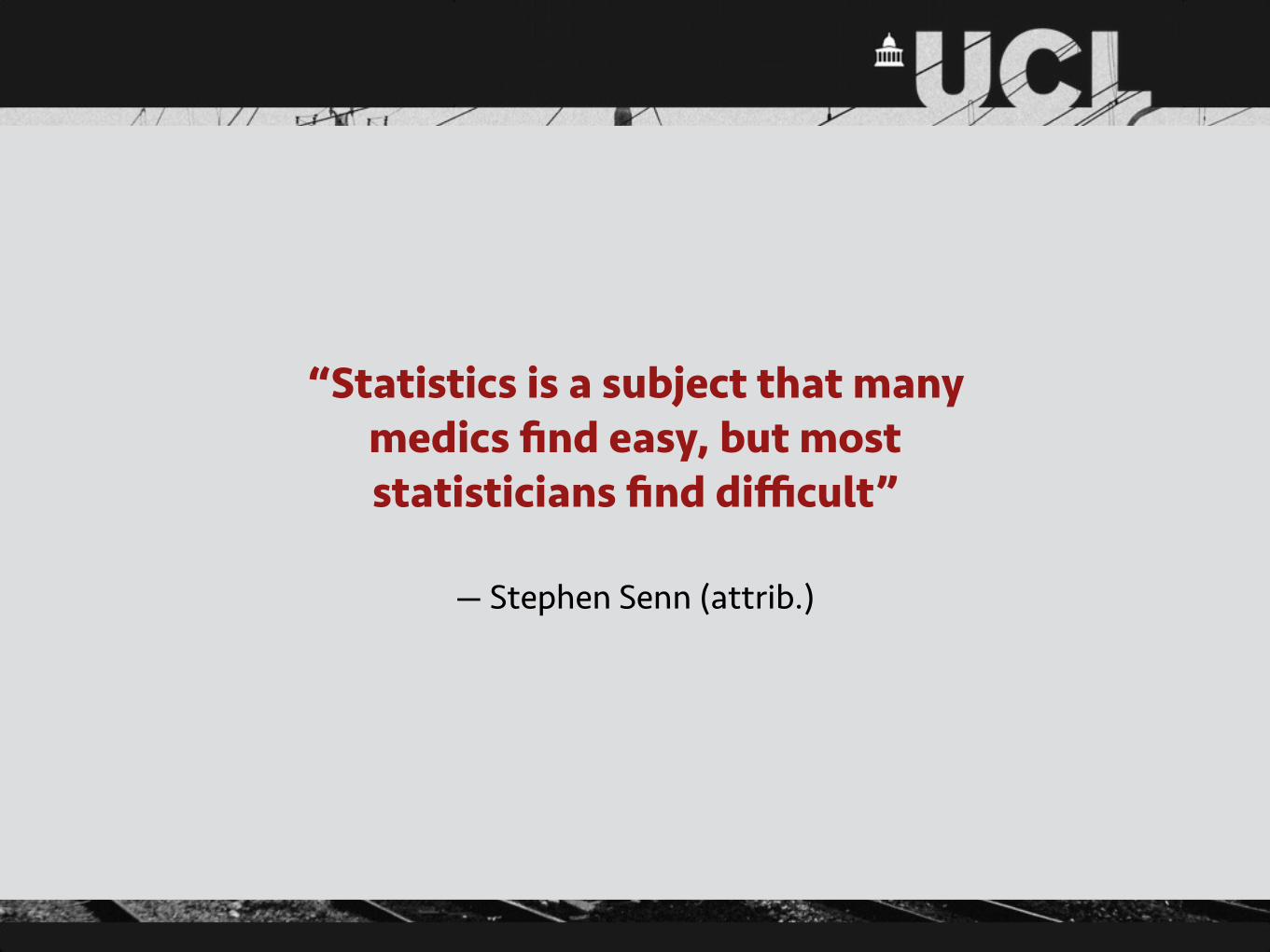
Purposes

• Summarising data, describing features such as central tendency and dispersion

• Making inferences about the population that a given sample was drawn from

Hypothesis testing• A null hypothesis is a default position (no effect, no difference, no

relationship, etc.)

• This is set against an alternative hypothesis, generally the opposite of the null

• A hypothesis test estimates the probability, p, of observing data at least as extreme as the sample, under the assumption that the null is true

• If this p-value is less than a threshold, α, usually 0.05, then the null is rejected and treated as false

• 5% of rejections are therefore expected to be false positives

• The rate at which the null hypothesis is correctly rejected is the power

• NB: Failing to reject the null hypothesis does not constitute strong evidence in support of it

The t-test• A test for a difference in means …

• … which may be of a particular sign (one-tailed) or either sign (two-tailed) …

• … either between two groups of observations (two sample), or one group and a fixed value, often zero (one sample) …

• … which is valid under the assumptions that the groups are approximately normally distributed, independently sampled and (for some implementations) have equal population variance

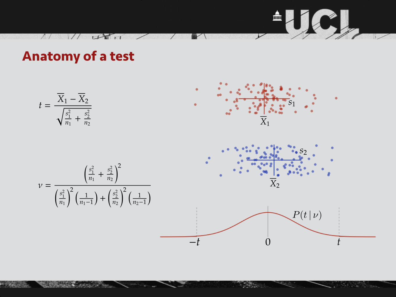
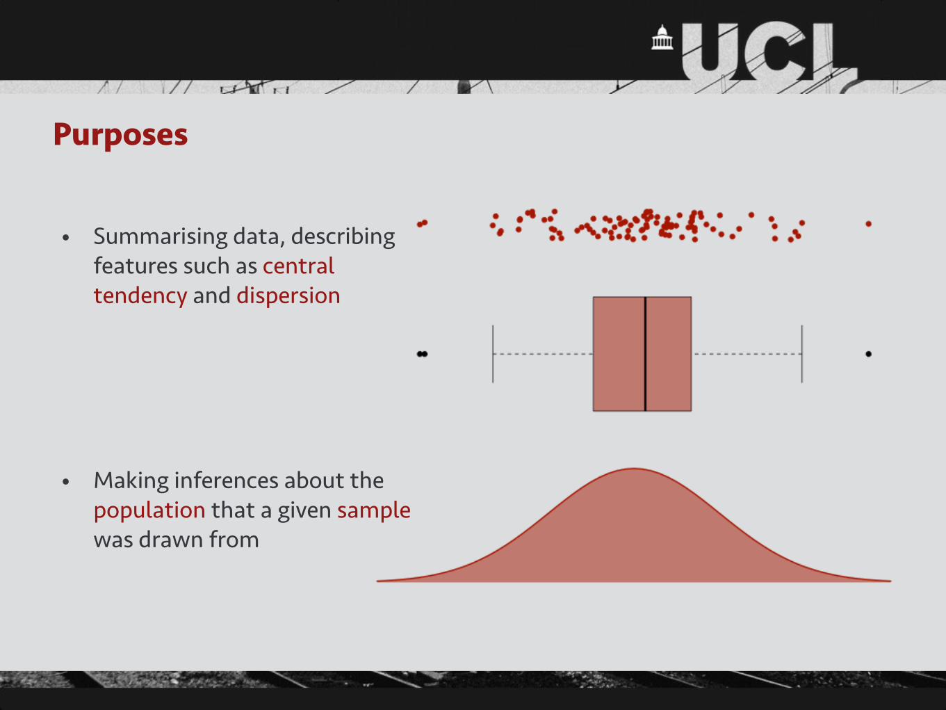
Anatomy of a test

t =X1 � X2q

s21

n1+

s22

n2

⌫ =

✓s2

1n1+

s22

n2

◆2

✓s2

1n1

◆2 ⇣1

n1�1

⌘+✓

s22

n2

◆2 ⇣1

n2�1

⌘

X1

X2

0 t�t

s1

s2

P (t | ⌫)

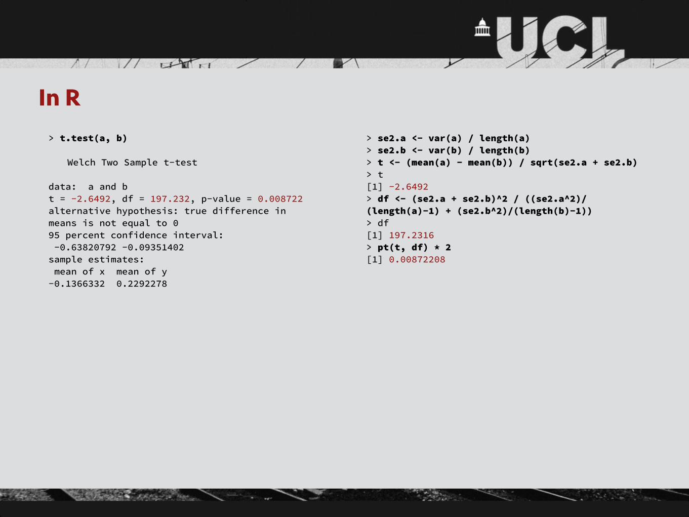
In R> t.test(a, b)

Welch Two Sample t-test

data: a and b t = -2.6492, df = 197.232, p-value = 0.008722 alternative hypothesis: true difference in means is not equal to 0 95 percent confidence interval: -0.63820792 -0.09351402 sample estimates: mean of x mean of y -0.1366332 0.2292278

> se2.a <- var(a) / length(a) > se2.b <- var(b) / length(b) > t <- (mean(a) - mean(b)) / sqrt(se2.a + se2.b) > t [1] -2.6492 > df <- (se2.a + se2.b)^2 / ((se2.a^2)/(length(a)-1) + (se2.b^2)/(length(b)-1)) > df [1] 197.2316 > pt(t, df) * 2 [1] 0.00872208

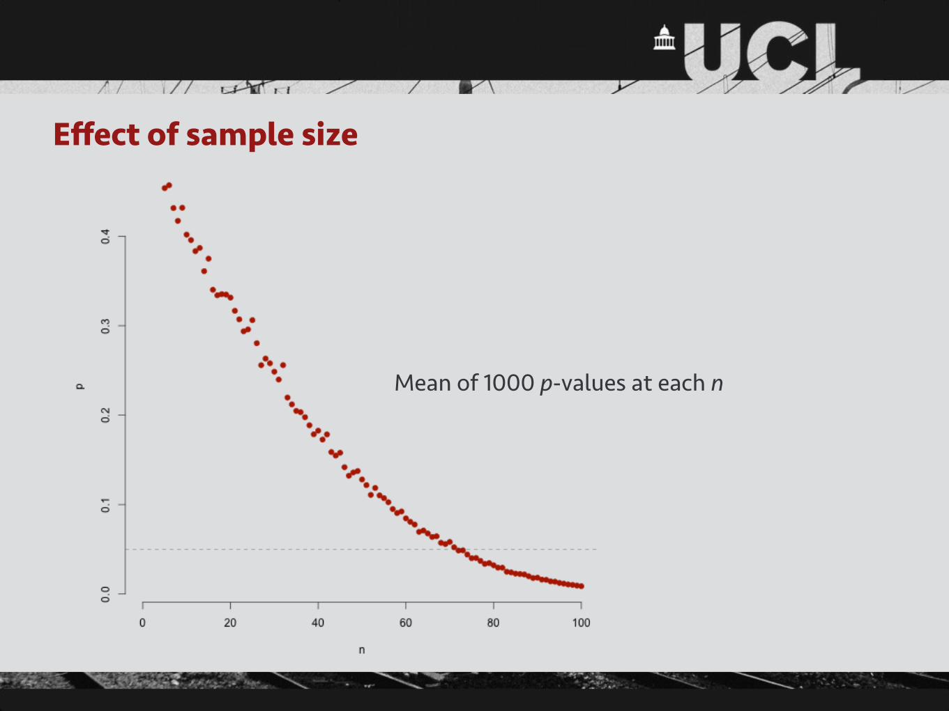
Effect of sample size

Mean of 1000 p-values at each n

Other common hypothesis tests• t-test for significant correlation coefficient

• t-test for significant regression coefficient

• F-test for difference between multiple means

• F-test for model comparison

• Nonparametric equivalents, e.g. signed-rank test

• Robustness to violations of assumptions varies

Issues with significance tests• Arbitrary p-value threshold

• Significance vs effect size, especially with many observations

• Publication bias: non-significant results are rarely published

• Choice of null hypothesis can be controversial

• Ignores any prior information

• Probability of data (obtained) vs probability that hypothesis is correct (often desired)

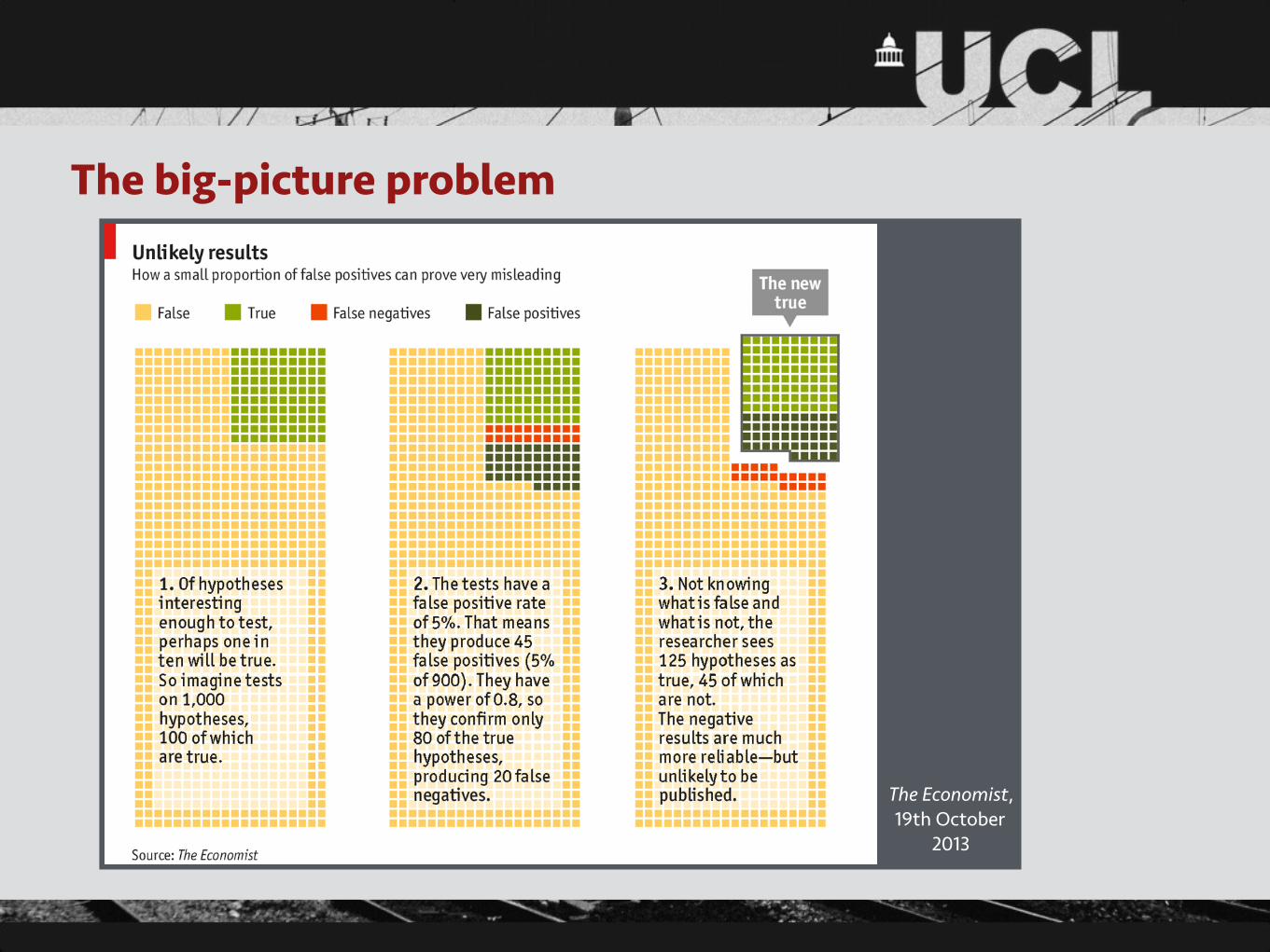
The big-picture problem

The Economist, 19th October

2013

Multiple comparisons

See R’s p.adjust function for p-value adjustments

The picture in imaging• Hypothesis tests may be performed on a variety of scales

• Worth carefully considering the appropriate scale for the research question

• Dimensionality reduction can be helpful

• Mass univariate testing (e.g. voxelwise) produces a major multiple comparisons issue

Linear (regression) models• We have some measurement, y, for each subject

• We have some predictor variables, x1, x2, x3, etc., for which we have measurements for each subject

• We want to know ß1, ß2, ß3, etc., the influences of each x on y

• We use the model

where the errors (or residuals), εi, are assumed to be normally distributed with zero mean

• Typically fitted with ordinary least squares, a simple matrix operation

• Assumes constant variance, independent errors, noncollinearity in predictors

y

i = �0 + �1x

i

1 + . . . + �p

x

i

p

+ "i

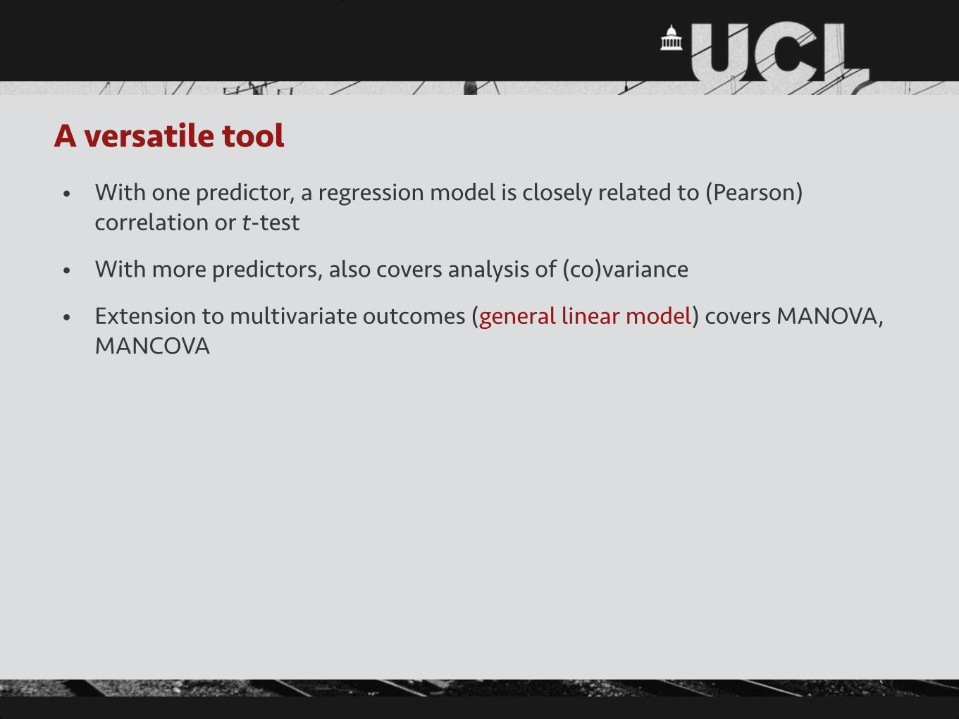
A versatile tool• With one predictor, a regression model is closely related to (Pearson)

correlation or t-test

• With more predictors, also covers analysis of (co)variance

• Extension to multivariate outcomes (general linear model) covers MANOVA, MANCOVA

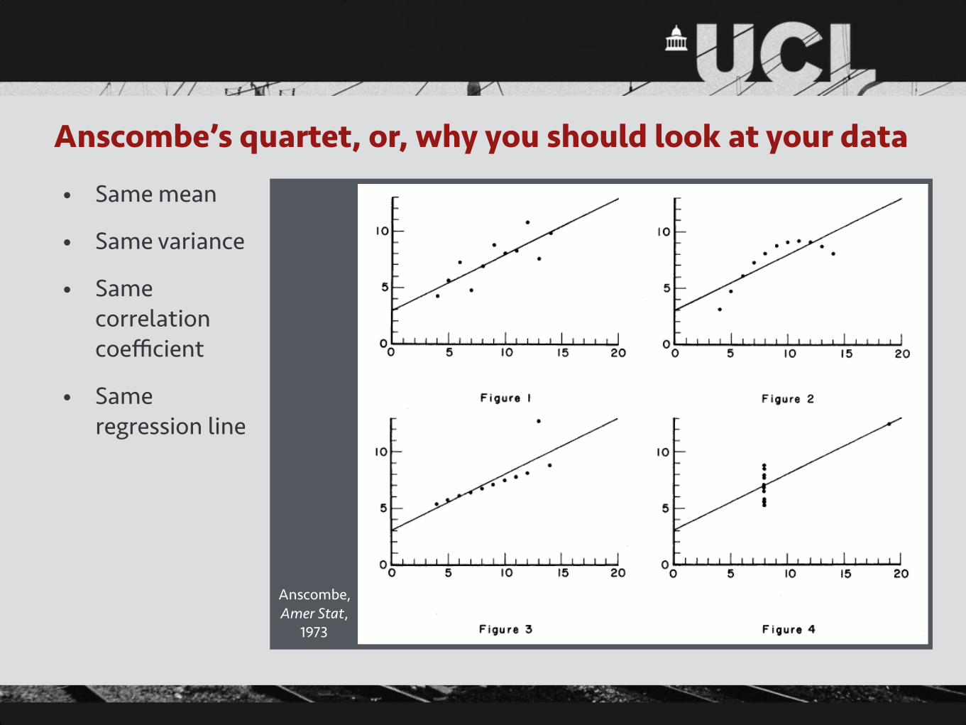
Anscombe’s quartet, or, why you should look at your data

• Same mean

• Same variance

• Same correlation coefficient

• Same regression line

Anscombe, Amer Stat,

1973

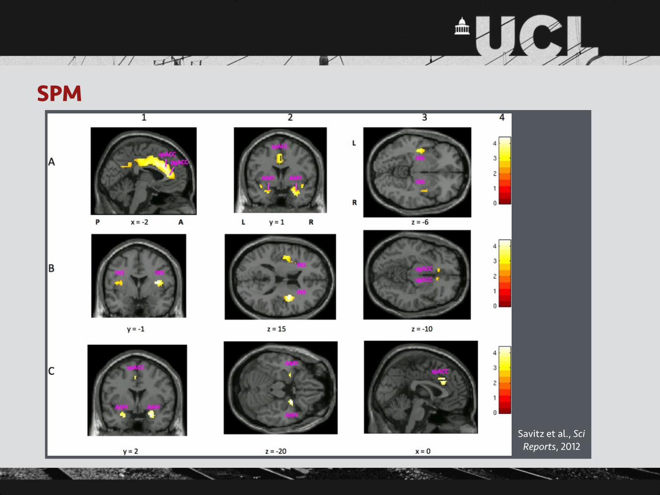
SPM

Savitz et al., Sci Reports, 2012

Beyond hypothesis tests• Models of data as outcomes, plus derivatives such as reference ranges

• Parameter estimates, confidences intervals, etc.

• Model comparison via likelihood, information theory approaches

• Clustering

• Predictive power, e.g. ROC analysis

• Measures of uncertainty via resampling methods

• Bayesian inference: prior and posterior distributions

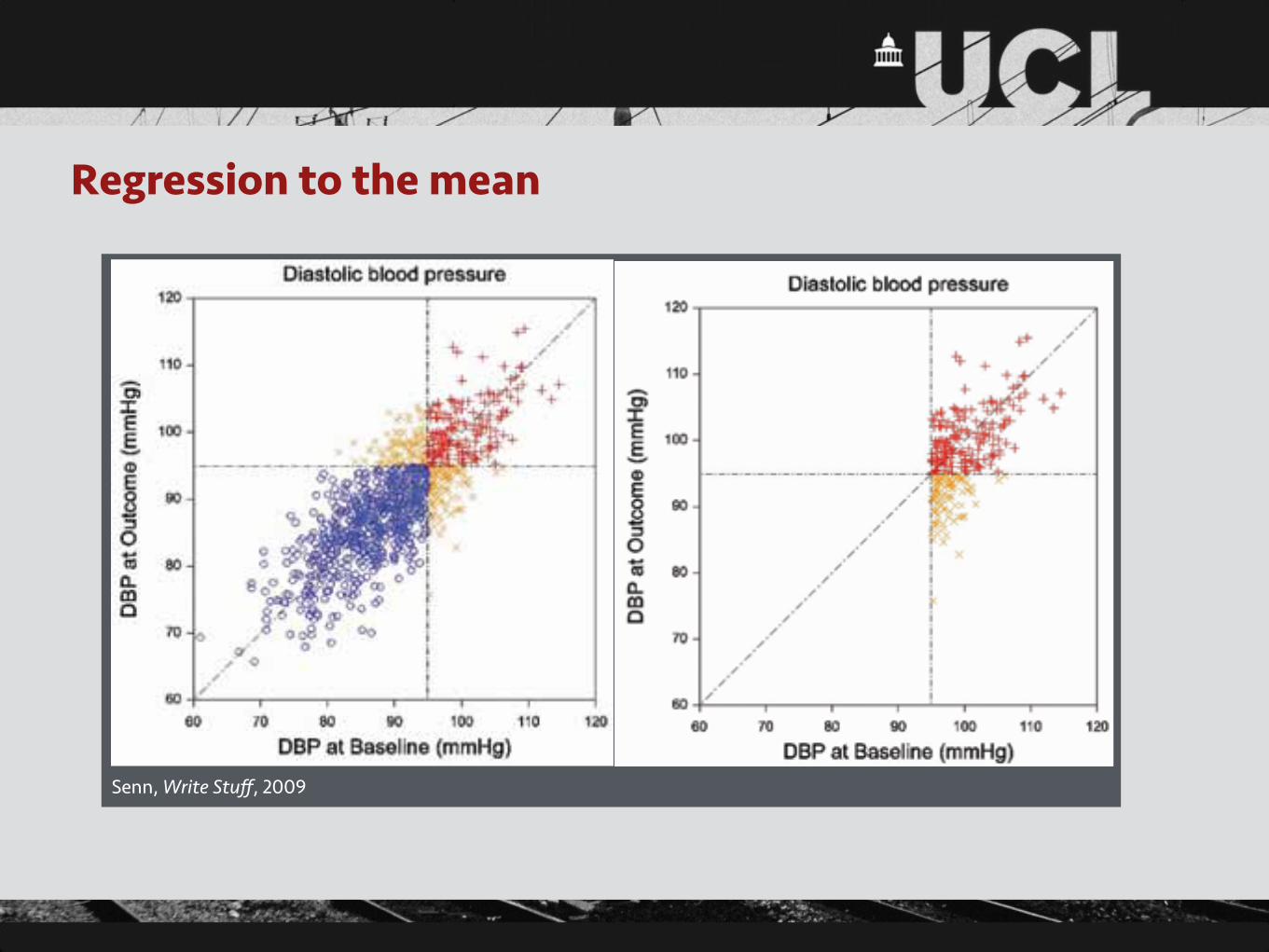
Regression to the mean

The Write StuffVol. 18, No. 3, 2009

The Journal of the European Medical Writers Association159

by Stephen Senn

Three things that every medical writer should know about statistics

IntroductionThe joke goes that there are three kind of statistician: those who can count and those who can’t. Therefore, readers of the Write Stuff will forgive me, I hope, if I end up writ-ing about more than three things. It should be obvious, in that case, as to which sort of statistician I am. There are, of course, many more things than three that every medi-cal writer should know about statistics because there are many things about statistics that anybody working in drug development should know and medical writers are in the unenviable position of having to know about everything. However, everybody has to start somewhere and three is a number with a great tradition. The three things I am going to write about are regression to the mean [1], the error of the transposed conditional [2] and individual response [3]. The first is a widespread phenomenon that has a powerful influence on the way that results appear to us, the second is a pernicious fallacy and the third is a sort of Holy Grail-cum-wild goose chase that is responsible for leading many a researcher astray.

Regression to the meanRegression to the mean is the tendency for members of a population who have been selected because they are ex-treme to be less extreme when measured again [4, 5]. Be-cause entry into clinical trials is usually only allowed if pa-tients have extreme values (diastolic blood pressure above 95 mmHg, Hamilton depression score greater than or equal to 22, forced expiratory volume in one second less than 75% of predicted etc.), regression to the mean is a phe-nomenon that is likely to affect many clinical trials. We can expect that patients will appear to improve even if the treat-ment is ineffective. Regression to the mean is a plausible explanation, for example, for the ‘placebo effect’ which then becomes, as I hope to explain, a purely statistical rath-er than psychological phenomenon.

How does it occur? Consider figure 1. This shows a simu-lated set of results for a group of 1000 individuals who have had their diastolic blood pressure (DBP) measured on two occasions: at ‘baseline’, X, and at ‘outcome’, Y. The figure plots Y against X and the simulation has been arranged so that the expected values of X and Y are identically equal to 90 mmHg and that the standard deviations are 8 mmHg with a correlation of 0.79. An arbitrary but common cut off of 95 mmHg is taken as being the boundary for hyperten-sion. Individuals are labelled as being of one of three sorts: hypertensive at both baseline and outcome (labelled with a red +), normotensive at both baseline and outcome (la-belled with a blue 0) and hypertensive on one occasion and not the other (labelled with an orange x).

Figure 1 Simulated results at baseline and outcome for diastolic blood pres-sure (mmHg) for 1000 individuals in a population.

Now consider a plot of a subset of the individuals, namely those who are ‘hypertensive’ on at least one occasion. This plot is given in figure 2. Just as was the case in figure 1 there is no essential difference as to whether we look at results at baseline or outcome, the mean result on either occasion, although higher than it was before because the ‘normotensives’ have been removed, will be the same.

Figure 2 Simulated results at baseline and outcome for diastolic blood pres-sure (mmHg) for 1000 individuals in a population with those who are normotensive on both occasions removed.

Vol. 18, No. 3, 2009The Write Stuff

The Journal of the European Medical Writers Association 160

Statistics: What medical writers should know

However, neither of these plots is what we would observe in a standard clinical trial. Instead, we would observe some-thing like figure 3. Figure 3 has been obtained from figure 2 by removing those patients who were normotensive at baseline but hypertensive at outcome. Why? Because if they were normotensive at baseline they would never be recruited into the trial and hence never followed up. Now we can see that the way that we have chosen subjects has an inherent bias if we measure the effect of treatment as the difference between outcome and baseline. The outcome values are on average lower than the baseline values but this is only because of the way that we have sampled. It says nothing about the effect of treatment.

Figure 3 Simulated results at baseline and outcome for diastolic blood pres-sure (mmHg) for 1000 individuals in a population with those who are normotensive at baseline removed.

The consequence is that on average patients will appear to improve even if the treatment is ineffective. In fact, patients given placebo can be expected to improve for reasons that are purely statistical. There is no need to invoke psycholo-gy, the healing hands of the physician, the white coat effect and so forth. The way that the data are collected suffices.

Does it matter? Not in a controlled clinical trial provided that we only consider, describe and interpret differences be-tween treatment and control groups. Both of these will be subject to the same regression to the mean effect, which is therefore eliminated by comparison. Hence, the joke about a medical statistician. If you ask him, “how’s your wife?” he answers, “compared to what?” Only head to head com-parisons have meaning. Alas, many clinical trial reports re-veal that trialists have no idea why they have carried out a controlled clinical trial. Pages of ink are wasted describing the response in each group, although this is meaningless. Reports would be sharper and understanding would be im-proved if these ignorant descriptions were dumped where they belong in the waste paper basket.

What are the lessons for a medical writer? He or she should think comparatively. Controlled clinical trials are about comparisons, or to use some statistical jargon treatment

contrasts, that is to say difference between treatments. Giv-en a choice between a graph that shows the course over time of each treatment together with standard error bars or a plot of the difference between treatments together with confidence interval for that difference, choose the latter and dump the former. If survival is the outcome of interest, it is the log-hazard ratio, a statistic used to model the difference between treatments, that should take pride of place and not the median survival within each group. For a binary out-come, stress the odds ratio rather than the probability for each group.

The error of the transposed conditionalAll French are Europeans but not all Europeans are French. I can put this in the language of probabilities. With a proba-bility of 100% someone who is French is European. Howev-er, the probability that a randomly chosen European (taking this to mean a citizen of the European Union) is French is only about 13% (since the population of France is about 65 million and that of the European Union about 500 million).

Here is another example. The probability that a randomly chosen woman has breast cancer is, thank goodness, quite low. However the probability that a randomly chosen breast cancer victim is a woman is extremely high. Or how about the prosecutor’s fallacy? The probability of the DNA on the scene of the crime matching that of the defendant is one in a million, therefore, claims the prosecution, there are 999,999 chances out of a million that he is guilty. However, in a population of 100 million (which could be the number of adult males in the USA) there must be 100 individuals about whom we could make a similar statement. They can’t all be almost certainly guilty.

This is all very obvious and elementary, yet, surprising-ly, even experienced trialists find it hard to grasp that the probability of A given B is not the same as the probabil-ity of B given A. Consider

that most ubiquitous of statistics, the P-value. A P-value is the probability of seeing a result as extreme or more ex-treme than that observed if the null hypothesis is true. In other words it says something about the probability of the evidence given the null hypothesis. It is not, therefore, the probability of the hypothesis given the evidence. Yet it is often misinterpreted as being the probability that the null hypothesis is true. This is just an egregious error.

P-values are a concept in frequentist statistics. The frequen-tist approach to statistics is the approach generally used in drug development. In this approach it is never possible to talk of the probability of a hypothesis being true. The hypothesis is either true or false. The problem is we don’t know which. If one wished to make statements about the truth of a hypothesis one would have to use the Bayesian

Patients given placebo can be expected to improve for reasons that are purely statistical

>

Senn, Write Stuff, 2009

Some advice• Plan ahead

• Be clear what you really want to know

• Use R

• Visualise and understand your data

• Save scripts

• Keep statistical tests to a minimum

• Be aware of sources of bias

• Use available resources at ICH and beyond