Statistics and DOE

ME 470Spring 2012

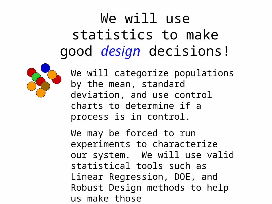
We will use statistics to make good design decisions!

We will categorize populations by the mean, standard deviation, and use control charts to determine if a process is in control.

We may be forced to run experiments to characterize our system. We will use valid statistical tools such as Linear Regression, DOE, and Robust Design methods to help us make those characterizations.

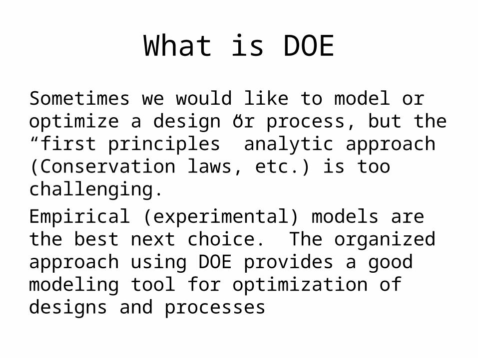
What is DOE

Sometimes we would like to model or optimize a design or process, but the “first principles” analytic approach (Conservation laws, etc.) is too challenging.Empirical (experimental) models are the best next choice. The organized approach using DOE provides a good modeling tool for optimization of designs and processes

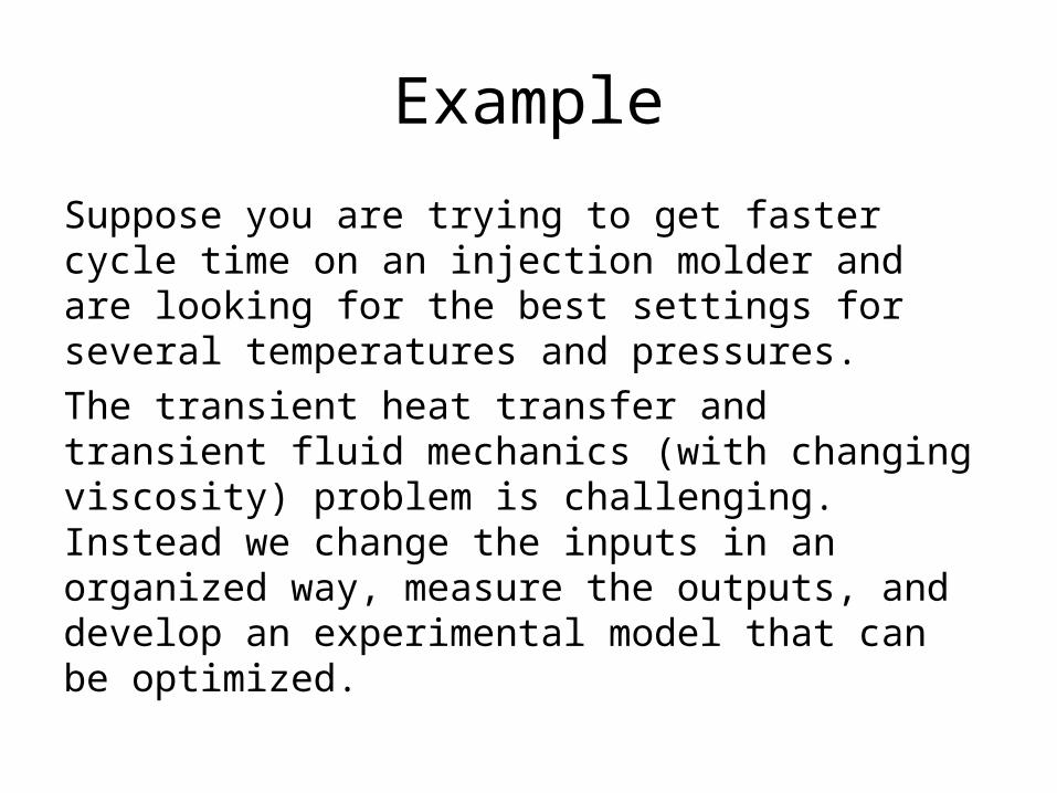
Example

Suppose you are trying to get faster cycle time on an injection molder and are looking for the best settings for several temperatures and pressures.The transient heat transfer and transient fluid mechanics (with changing viscosity) problem is challenging. Instead we change the inputs in an organized way, measure the outputs, and develop an experimental model that can be optimized.

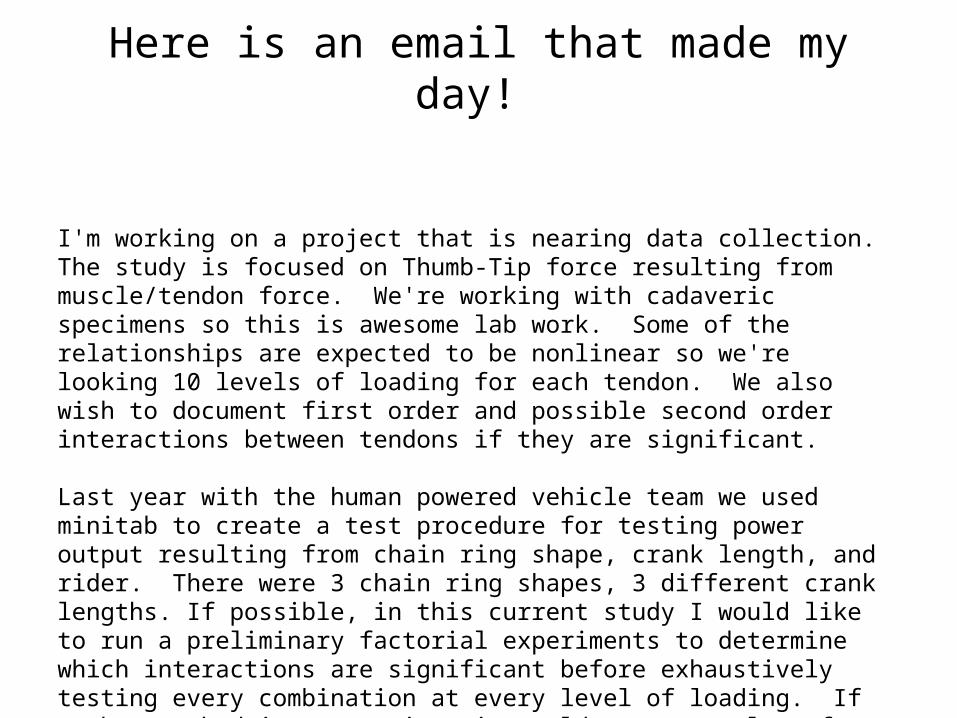
Here is an email that made my day!

I'm working on a project that is nearing data collection.  The study is focused on Thumb-Tip force resulting from muscle/tendon force.  We're working with cadaveric specimens so this is awesome lab work.  Some of the relationships are expected to be nonlinear so we're looking 10 levels of loading for each tendon.  We also wish to document first order and possible second order interactions between tendons if they are significant.

Last year with the human powered vehicle team we used minitab to create a test procedure for testing power output resulting from chain ring shape, crank length, and rider.  There were 3 chain ring shapes, 3 different crank lengths. If possible, in this current study I would like to run a preliminary factorial experiments to determine which interactions are significant before exhaustively testing every combination at every level of loading.  If such a method is appropriate it could save us a lot of time.  Could you suggest a reference that I might be able to find at the library or on amazon?

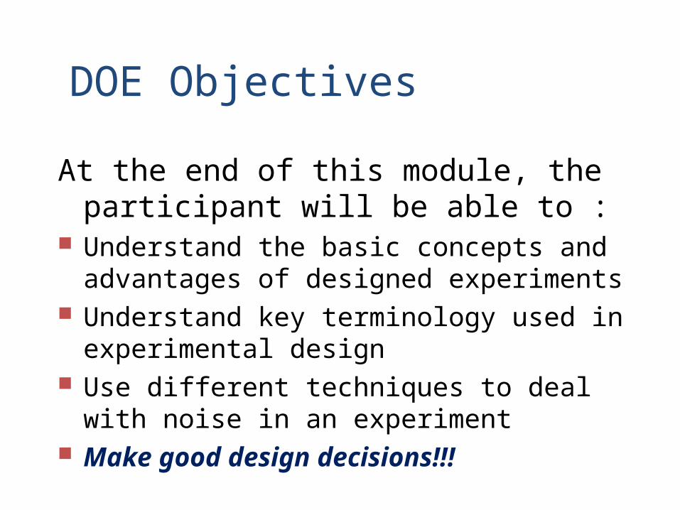
DOE Objectives

At the end of this module, the participant will be able to :

Understand the basic concepts and advantages of designed experiments

Understand key terminology used in experimental design

Use different techniques to deal with noise in an experiment

Make good design decisions!!!

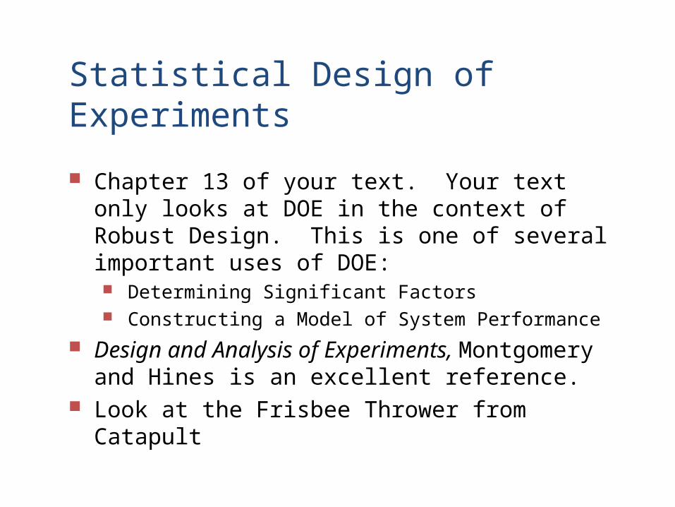
Statistical Design of Experiments

Chapter 13 of your text. Your text only looks at DOE in the context of Robust Design. This is one of several important uses of DOE: Determining Significant Factors Constructing a Model of System Performance

Design and Analysis of Experiments, Montgomery and Hines is an excellent reference.

Look at the Frisbee Thrower from Catapult

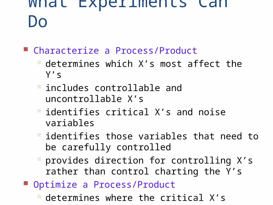
What Experiments Can Do

Characterize a Process/Product determines which X’s most affect the Y’s includes controllable and uncontrollable X’s identifies critical X’s and noise variables identifies those variables that need to be carefully

controlled provides direction for controlling X’s rather than control

charting the Y’s Optimize a Process/Product

determines where the critical X’s should be set determines “real” specification limits provides direction for “robust” designs

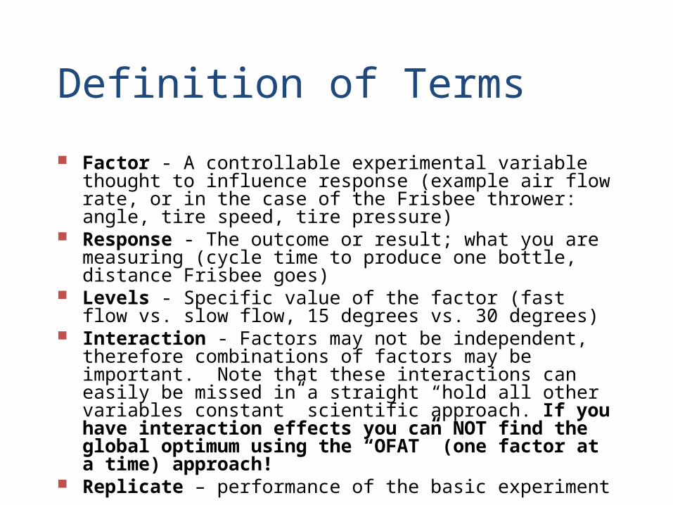
Definition of Terms

Factor - A controllable experimental variable thought to influence response (example air flow rate, or in the case of the Frisbee thrower: angle, tire speed, tire pressure)

Response - The outcome or result; what you are measuring (cycle time to produce one bottle, distance Frisbee goes)

Levels - Specific value of the factor (fast flow vs. slow flow, 15 degrees vs. 30 degrees)

Interaction - Factors may not be independent, therefore combinations of factors may be important. Note that these interactions can easily be missed in a straight “hold all other variables constant” scientific approach. If you have interaction effects you can NOT find the global optimum using the “OFAT” (one factor at a time) approach!

Replicate – performance of the basic experiment

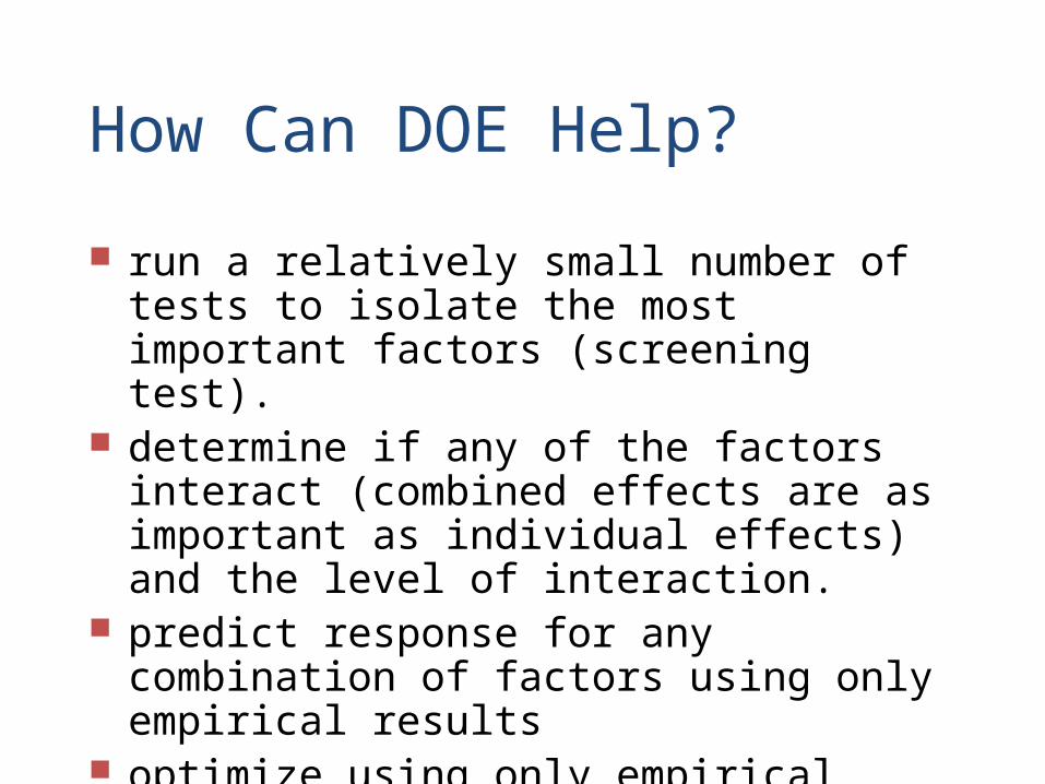
How Can DOE Help?

run a relatively small number of tests to isolate the most important factors (screening test).

determine if any of the factors interact (combined effects are as important as individual effects) and the level of interaction.

predict response for any combination of factors using only empirical results

optimize using only empirical results determine the design space for simulation models

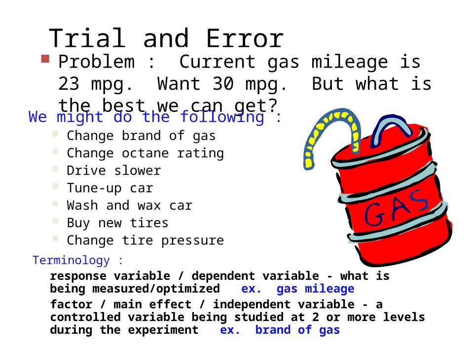
Trial and Error Problem : Current gas mileage is 23 mpg. Want 30

mpg. But what is the best we can get?

We might do the following : Change brand of gas Change octane rating Drive slower Tune-up car Wash and wax car Buy new tires Change tire pressure

Terminology :response variable / dependent variable - what is being measured/optimized ex. gas mileagefactor / main effect / independent variable - a controlled variable being studied at 2 or more levels during the experiment ex. brand of gas

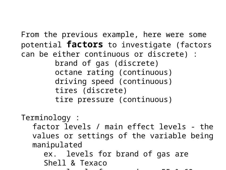
From the previous example, here were some potential factors to investigate (factors can be either continuous or discrete) :

brand of gas (discrete)octane rating (continuous)driving speed (continuous)tires (discrete)tire pressure (continuous)

Terminology :factor levels / main effect levels - the values or settings of the variable being manipulated

ex. levels for brand of gas are Shell & Texacoex. levels for speed are 55 & 60ex. levels for octane are 85 & 90

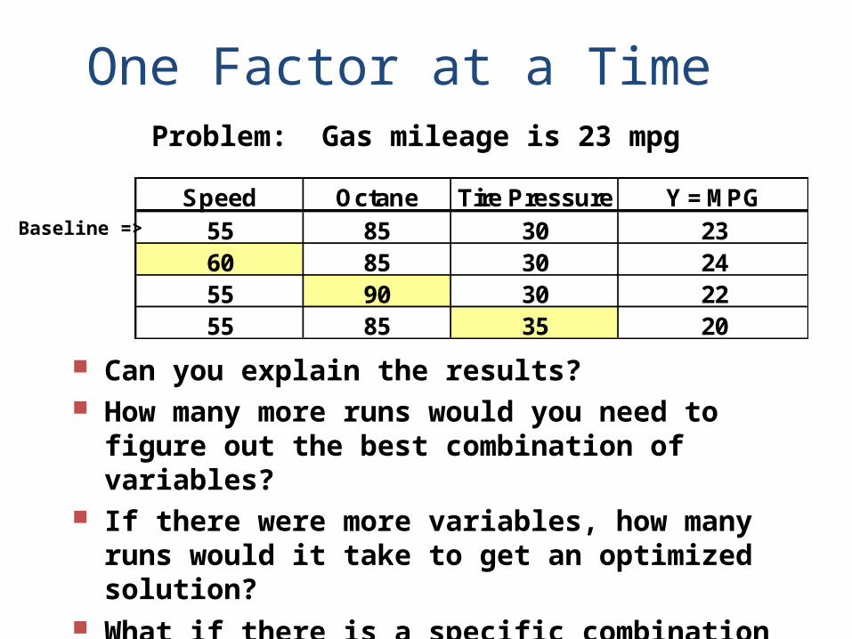
One Factor at a Time

Can you explain the results? How many more runs would you need to figure out the

best combination of variables? If there were more variables, how many runs would it

take to get an optimized solution? What if there is a specific combination of two or more

variables that leads to the best mpg?

Problem: Gas mileage is 23 mpg

Speed Octane Tire Pressure Y = MPG55 85 30 2360 85 30 2455 90 30 2255 85 35 20

Baseline =>

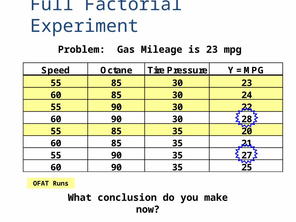
Full Factorial Experiment

OFAT Runs

Problem: Gas Mileage is 23 mpg

What conclusion do you make now?

Speed Octane Tire Pressure Y = MPG55 85 30 2360 85 30 2455 90 30 2260 90 30 2855 85 35 2060 85 35 2155 90 35 2760 90 35 25

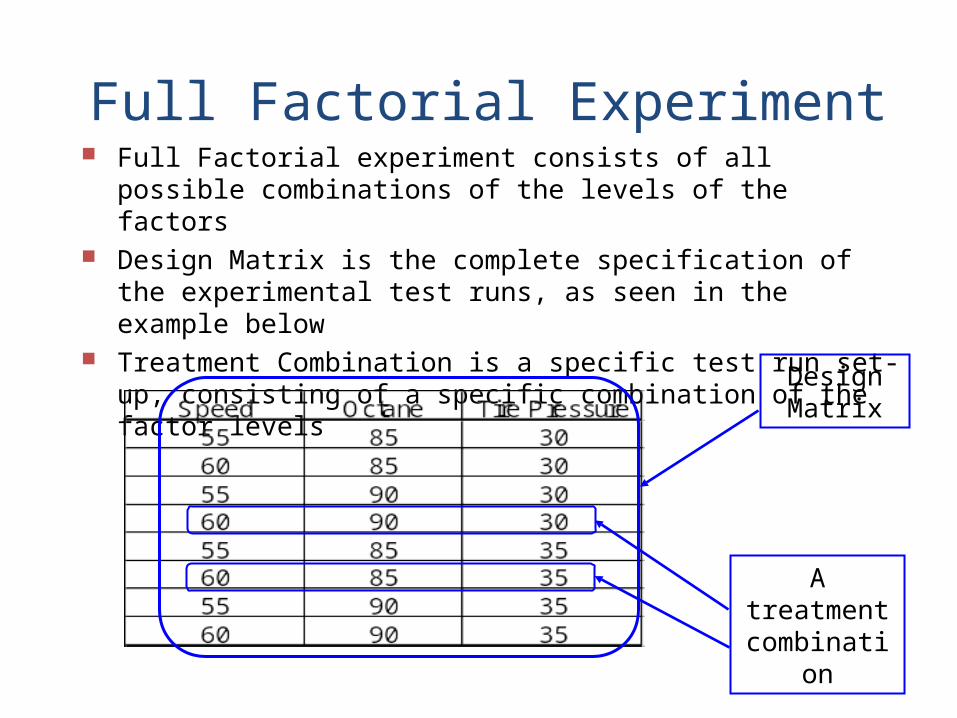
Full Factorial Experiment Full Factorial experiment consists of all possible combinations of the

levels of the factors Design Matrix is the complete specification of the experimental test runs,

as seen in the example below Treatment Combination is a specific test run set-up, consisting of a

specific combination of the factor levels

Design Matrix

A treatment combination

What makes up an experiment?

Response Variable(s) Factors Randomization Repetition and Replication

Response Variable

The variable that is measured and the object of the characterization or optimization (the Y)

Defining the response variable can be difficult Often selected due to ease of measurement Some questions to ask :

How will the results be quantified/analyzed? How good is the measurement system? What are the baseline mean and standard deviation? How big of a change do we care about? Are there several response variables of interest?

Factor

A variable which is controlled or varied in a systematic way during the experiment (the X)

Tested at 2 or more levels to observe its effect on the response variable(s) (Ys)

Some questions to ask : what are reasonable ranges to ensure a change in Y? knowledge of relationship, i.e. linear or quadratic, etc?

Examples material, supplier, EGR rate, injection timing can you think of others?

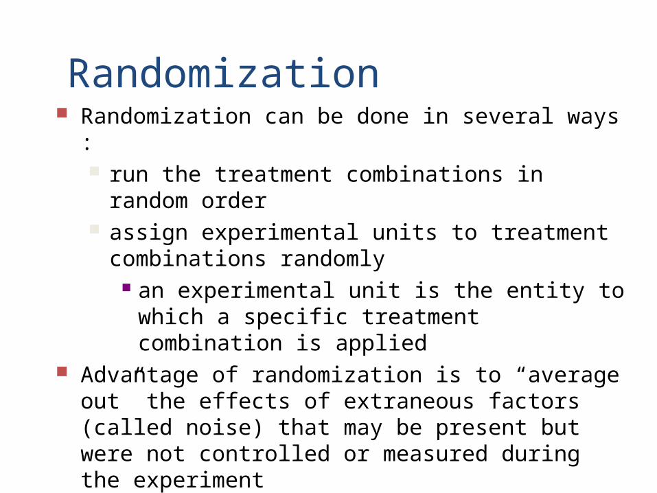
Randomization Randomization can be done in several ways :

run the treatment combinations in random order assign experimental units to treatment combinations

randomly an experimental unit is the entity to which a specific

treatment combination is applied Advantage of randomization is to “average out” the effects of

extraneous factors (called noise) that may be present but were not controlled or measured during the experiment spread the effect of the noise across all runs these extraneous factors (noise) cause unexplained

variation in the response variable(s)

Repetition and Replication

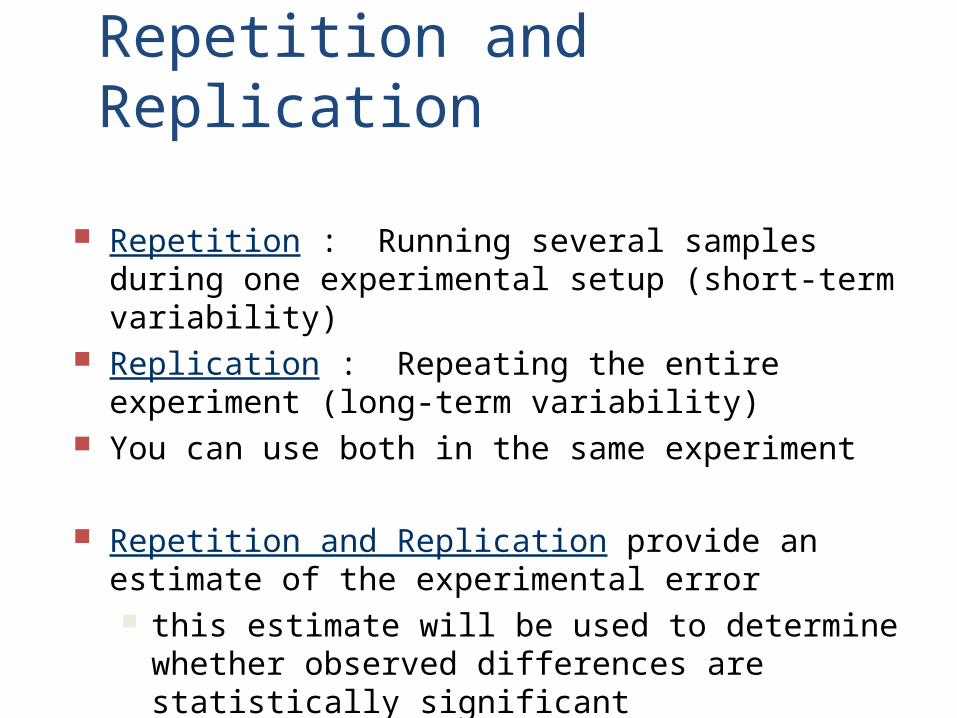
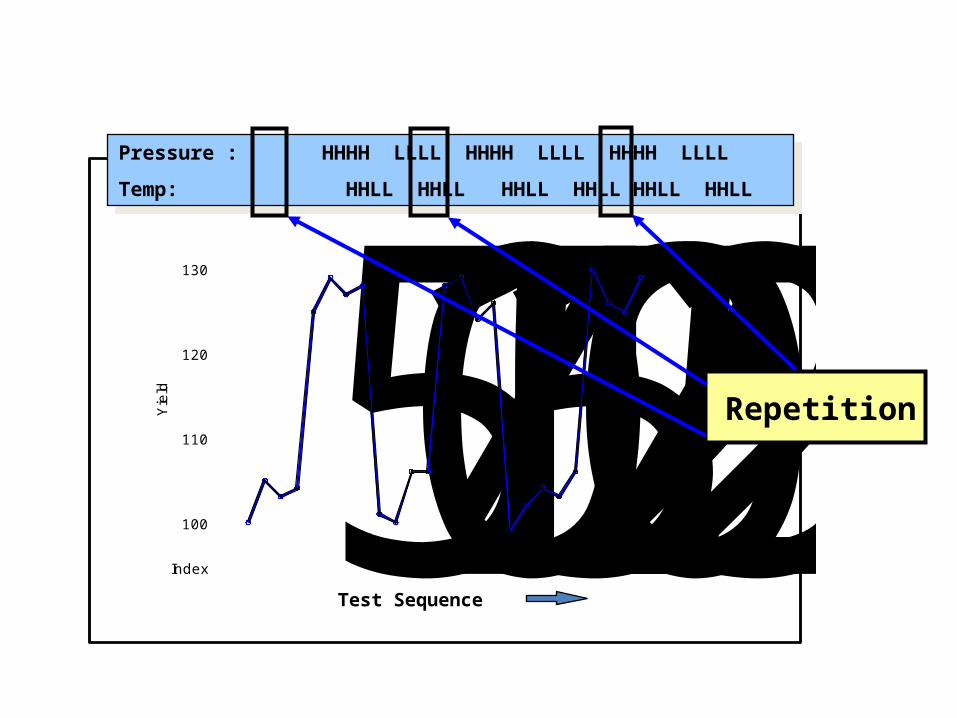
Repetition : Running several samples during one experimental setup (short-term variability)

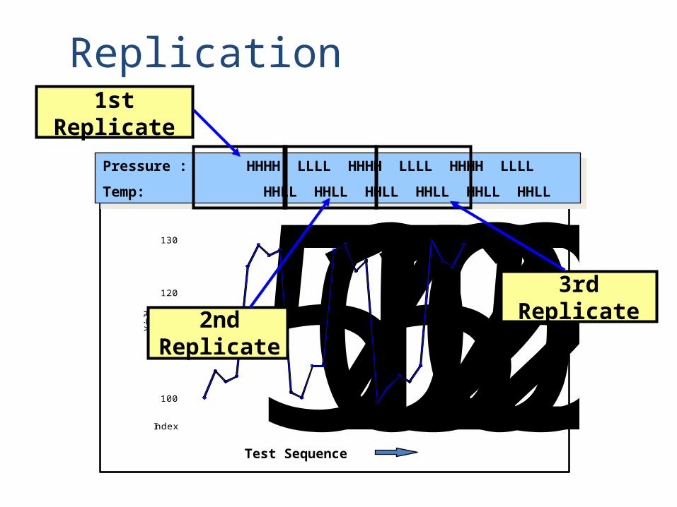
Replication : Repeating the entire experiment (long-term variability)

You can use both in the same experiment

Repetition and Replication provide an estimate of the experimental error this estimate will be used to determine whether observed

differences are statistically significant

252015105130

120

110

100

Index

Yie

ldPressure : HHHH LLLL HHHH LLLL HHHH LLLL

Temp: HHLL HHLL HHLL HHLL HHLL HHLL

Pressure : HHHH LLLL HHHH LLLL HHHH LLLL

Temp: HHLL HHLL HHLL HHLL HHLL HHLL

Test Sequence

Repetition

Replication

252015105130

120

110

100

Index

Yie

ld

Pressure : HHHH LLLL HHHH LLLL HHHH LLLL

Temp: HHLL HHLL HHLL HHLL HHLL HHLL

Pressure : HHHH LLLL HHHH LLLL HHHH LLLL

Temp: HHLL HHLL HHLL HHLL HHLL HHLL

Test Sequence

3rdReplicate2nd

Replicate

1stReplicate

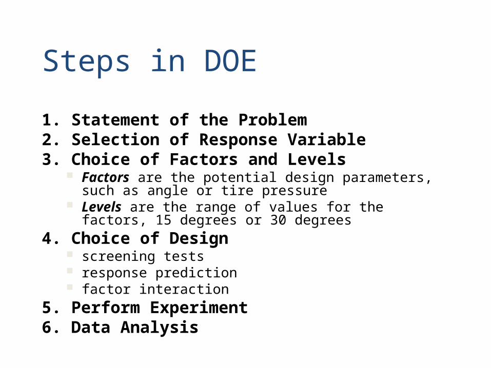
Steps in DOE

1. Statement of the Problem2. Selection of Response Variable 3. Choice of Factors and Levels

Factors are the potential design parameters, such as angle or tire pressure

Levels are the range of values for the factors, 15 degrees or 30 degrees

4. Choice of Design screening tests response prediction  factor interaction

5. Perform Experiment6. Data Analysis

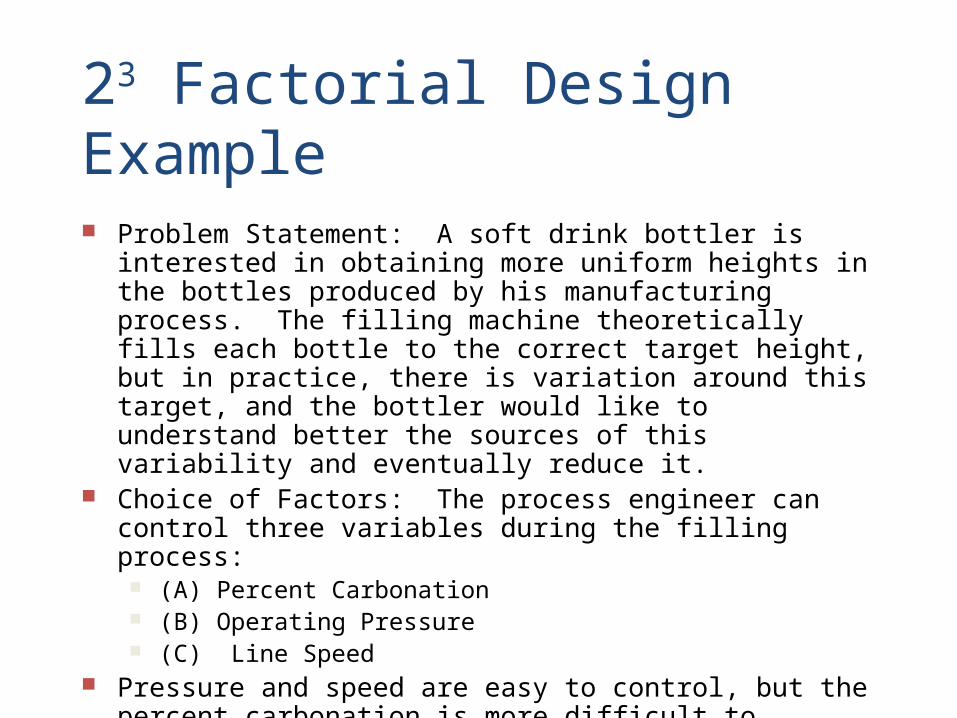
23 Factorial Design Example

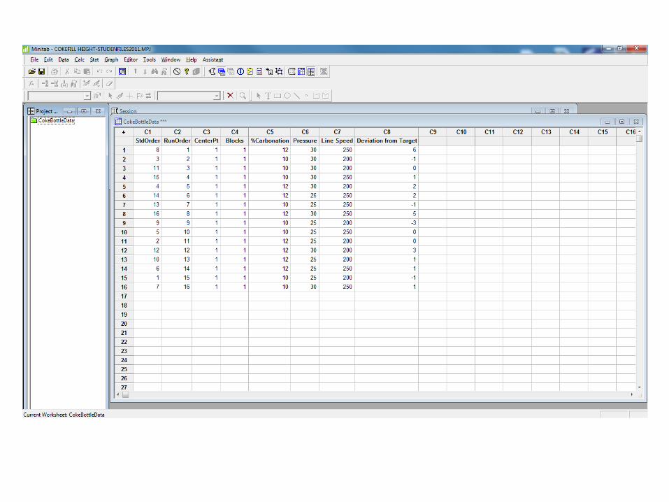
Problem Statement: A soft drink bottler is interested in obtaining more uniform heights in the bottles produced by his manufacturing process. The filling machine theoretically fills each bottle to the correct target height, but in practice, there is variation around this target, and the bottler would like to understand better the sources of this variability and eventually reduce it.

Choice of Factors: The process engineer can control three variables during the filling process: (A) Percent Carbonation (B) Operating Pressure (C) Line Speed

Pressure and speed are easy to control, but the percent carbonation is more difficult to control during actual manufacturing because it varies with product temperature.

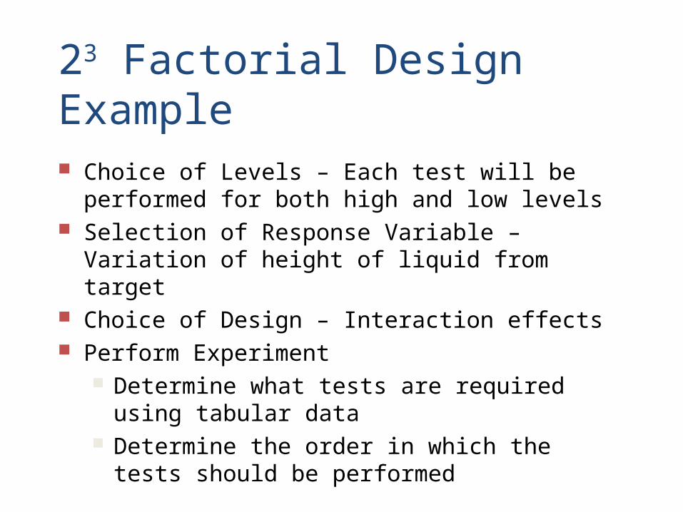
23 Factorial Design Example

Choice of Levels – Each test will be performed for both high and low levels

Selection of Response Variable – Variation of height of liquid from target

Choice of Design – Interaction effects Perform Experiment

Determine what tests are required using tabular data Determine the order in which the tests should be

performed

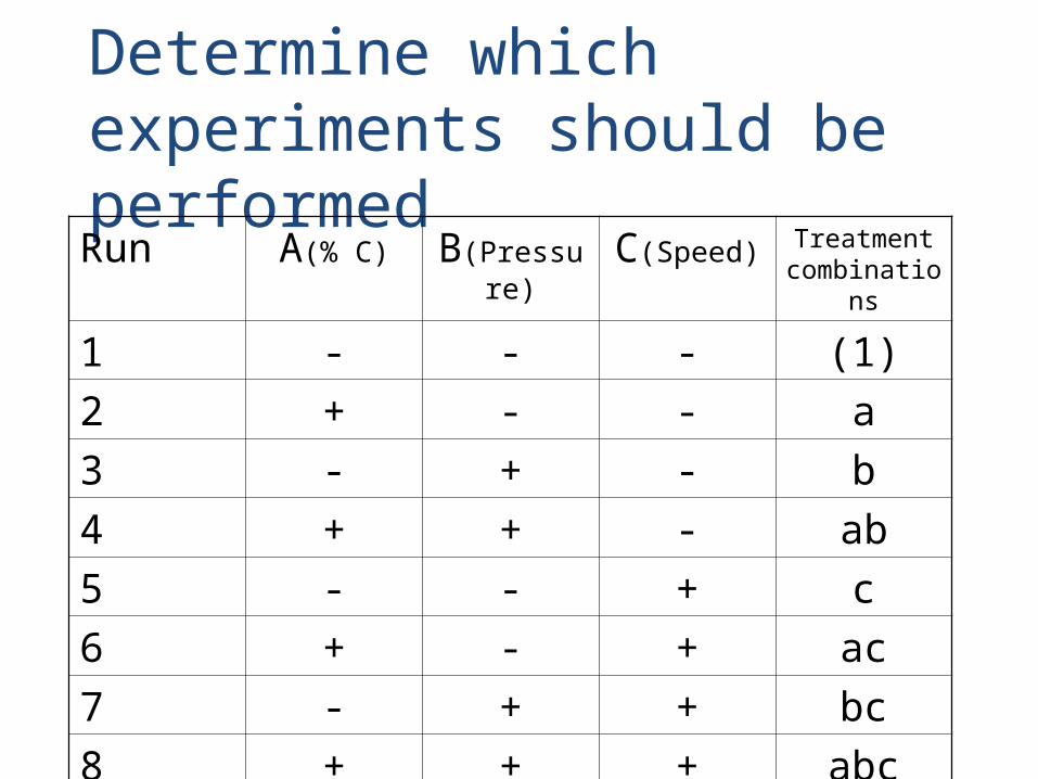
Determine which experiments should be performedRun A(% C) B(Pressure) C(Speed) Treatment

combinations

1 - - - (1)

2 + - - a

3 - + - b

4 + + - ab

5 - - + c

6 + - + ac

7 - + + bc

8 + + + abc

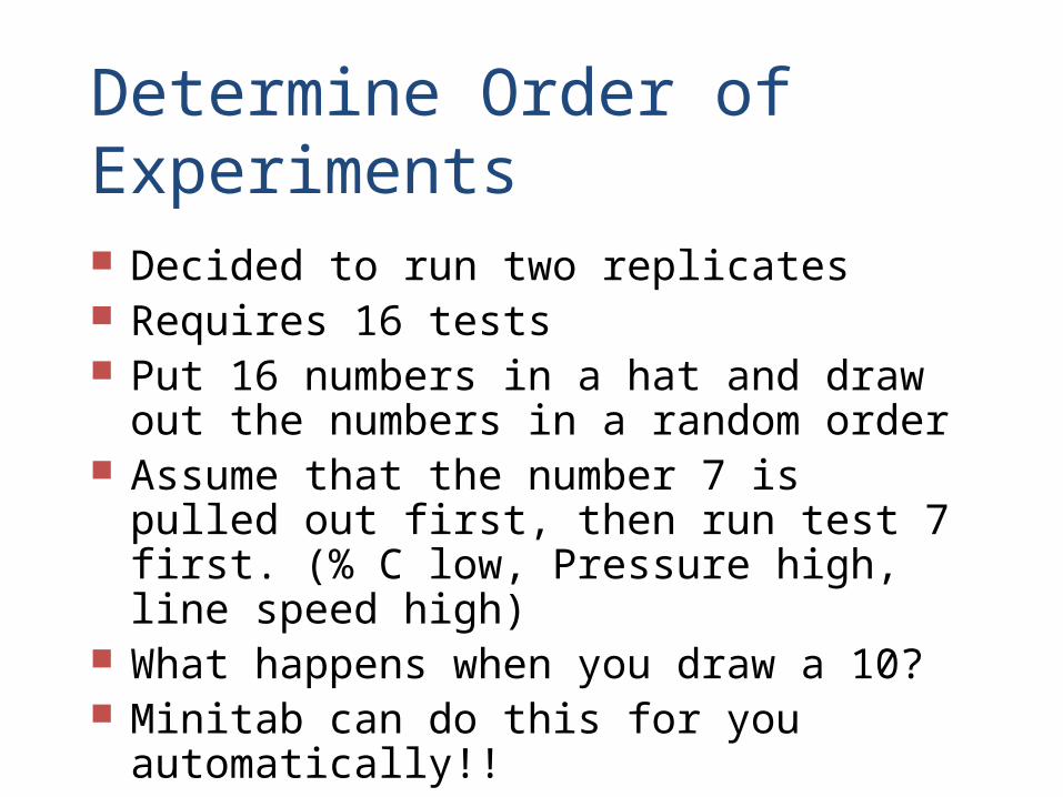
Determine Order of Experiments

Decided to run two replicates Requires 16 tests Put 16 numbers in a hat and draw out the numbers

in a random order Assume that the number 7 is pulled out first, then

run test 7 first. (% C low, Pressure high, line speed high)

What happens when you draw a 10? Minitab can do this for you automatically!!

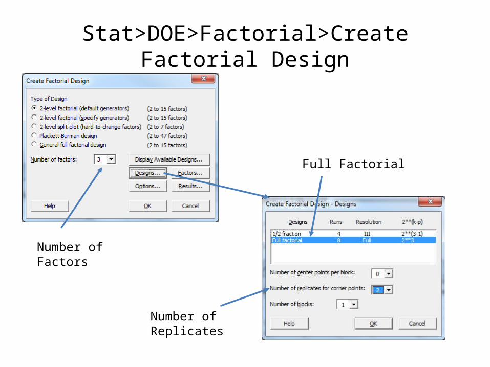
Stat>DOE>Factorial>Create Factorial Design

Full Factorial

Number ofReplicates

Number ofFactors

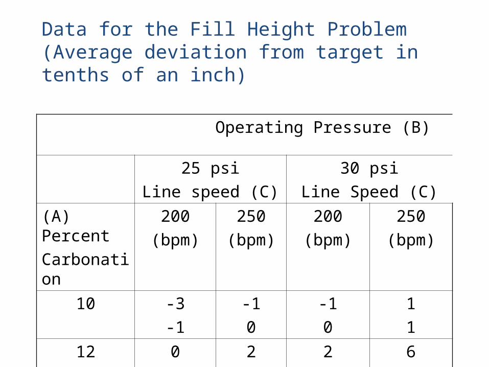
Data for the Fill Height Problem(Average deviation from target in tenths of an inch)

Operating Pressure (B)

25 psi

Line speed (C)

30 psi

Line Speed (C)

(A) Percent

Carbonation

200

(bpm)

250

(bpm)

200

(bpm)

250

(bpm)

10 -3

-1

-1

0

-1

0

1

1

12 0

1

2

1

2

3

6

5

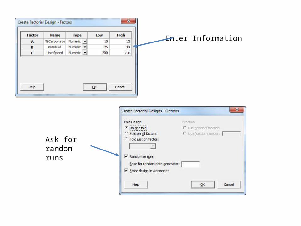
Enter Information

Ask for random runs

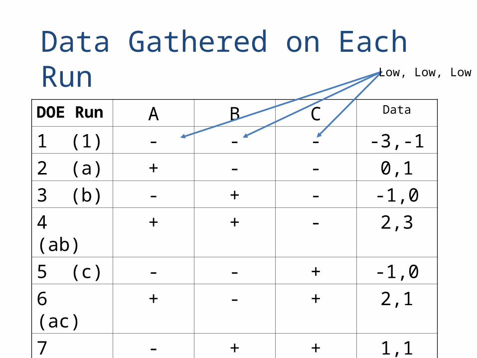
Data Gathered on Each Run

DOE Run A B C Data

1 (1) - - - -3,-1

2 (a) + - - 0,1

3 (b) - + - -1,0

4 (ab) + + - 2,3

5 (c) - - + -1,0

6 (ac) + - + 2,1

7 (bc) - + + 1,1

8 (abc) + + + 6,5

Low, Low, Low

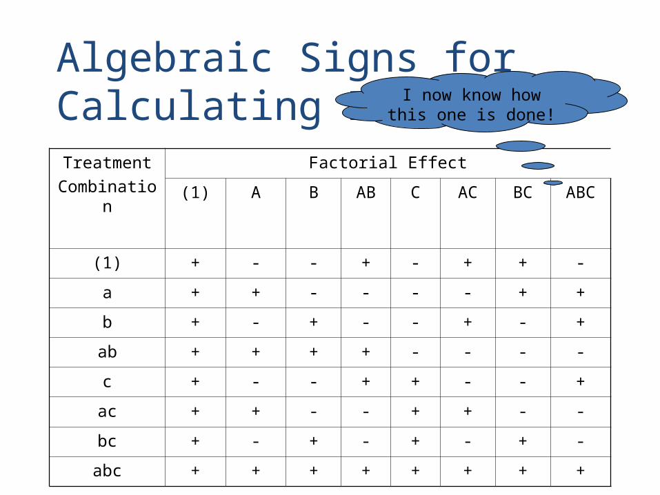
Algebraic Signs for Calculating Effects

Treatment

Combination

Factorial Effect

(1) A B AB C AC BC ABC

(1) + - - + - + + -

a + + - - - - + +

b + - + - - + - +

ab + + + + - - - -

c + - - + + - - +

ac + + - - + + - -

bc + - + - + - + -

abc + + + + + + + +

I now know how this one is done!

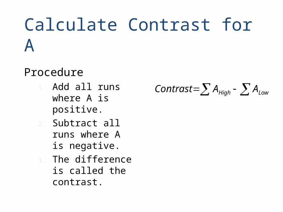
Calculate Contrast for A

Procedure1. Add all runs where A

is positive.

2. Subtract all runs where A is negative.

3. The difference is called the contrast.

LowHigh AAContrast

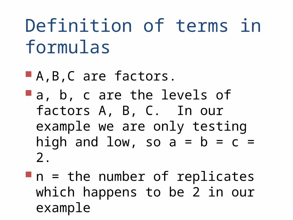
Definition of terms in formulas

A,B,C are factors. a, b, c are the levels of factors A, B, C. In

our example we are only testing high and low, so a = b = c = 2.

n = the number of replicates which happens to be 2 in our example

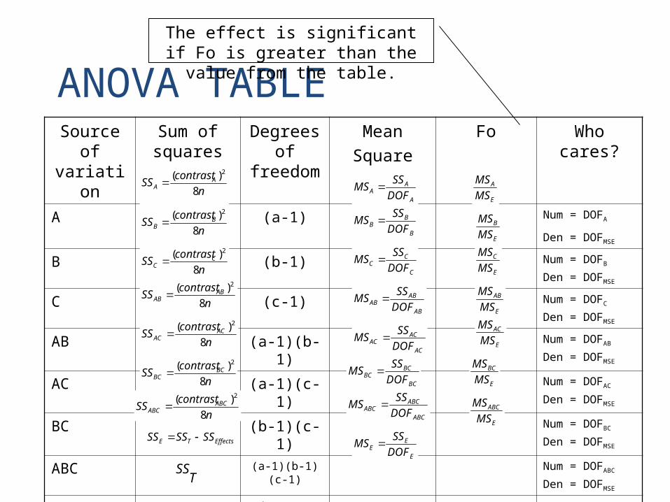
ANOVA TABLESource of variation

Sum of squares

Degrees of freedom

Mean

Square

Fo Who cares?

A (a-1) Num = DOFA

Den = DOFMSE

B (b-1) Num = DOFB

Den = DOFMSE

C (c-1) Num = DOFC

Den = DOFMSE

AB (a-1)(b-1) Num = DOFAB

Den = DOFMSE

AC (a-1)(c-1) Num = DOFAC

Den = DOFMSE

BC (b-1)(c-1) Num = DOFBC

Den = DOFMSE

ABC (a-1)(b-1)(c-1) Num = DOFABC

Den = DOFMSE

Error abc(n-1)

Total abcn-1

n

contrastSS A

A 8

)( 2

A

AA DOF

SSMS

TSS

n

contrastSS B

B 8

)( 2

n

contrastSS BC

BC 8

)( 2

n

contrastSS AC

AC 8

)( 2

n

contrastSS ABC

ABC 8

)( 2

n

contrastSS C

C 8

)( 2

n

contrastSS AB

AB 8

)( 2

B

BB DOF

SSMS

C

CC DOF

SSMS

BA

ABAB DOF

SSMS

AC

ACAC DOF

SSMS

BC

BCBC DOF

SSMS

ABC

ABCABC DOF

SSMS

E

EE DOF

SSMS EffectsTE SSSSSS

E

A

MS

MS

E

B

MS

MS

E

C

MS

MS

E

AB

MS

MS

E

AC

MS

MS

E

BC

MS

MS

E

ABC

MS

MS

The effect is significant if Fo is greater than the value from the table.

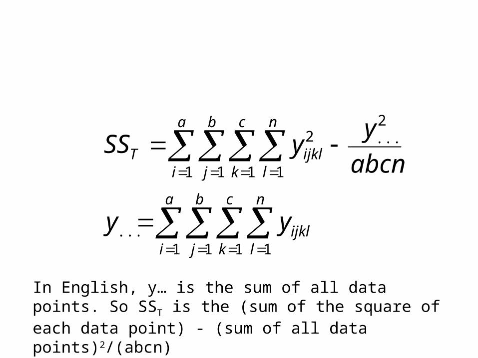
a

i

b

j

c

k

n

lijkl

a

i

b

j

c

k

n

lijklT

yy

abcn

yySS

1 1 1 1...

2...

1 1 1 1

2

In English, y… is the sum of all data points. So SST is the (sum of the square of each data point) - (sum of all data points)2/(abcn)

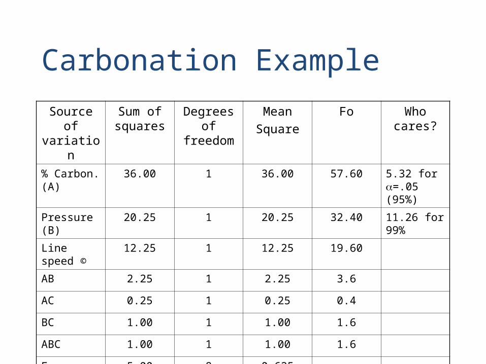
Carbonation Example

Source of variation

Sum of squares

Degrees of freedom

Mean

Square

Fo Who cares?

% Carbon. (A)

36.00 1 36.00 57.60 5.32 for =.05 (95%)

Pressure (B) 20.25 1 20.25 32.40 11.26 for 99%

Line speed © 12.25 1 12.25 19.60

AB 2.25 1 2.25 3.6

AC 0.25 1 0.25 0.4

BC 1.00 1 1.00 1.6

ABC 1.00 1 1.00 1.6

Error 5.00 8 0.625

Total 78.00 15

I don’t want to do all of the math

• Can I get Minitab to do it for me?

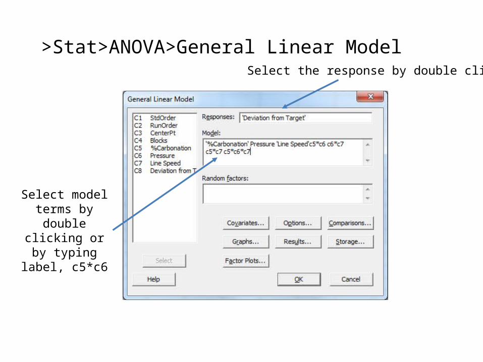
>Stat>ANOVA>General Linear ModelSelect the response by double clicking

Select model terms by double clicking or by typing label,

c5*c6

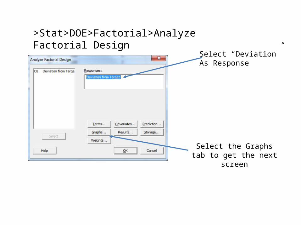
>Stat>DOE>Factorial>Analyze Factorial Design

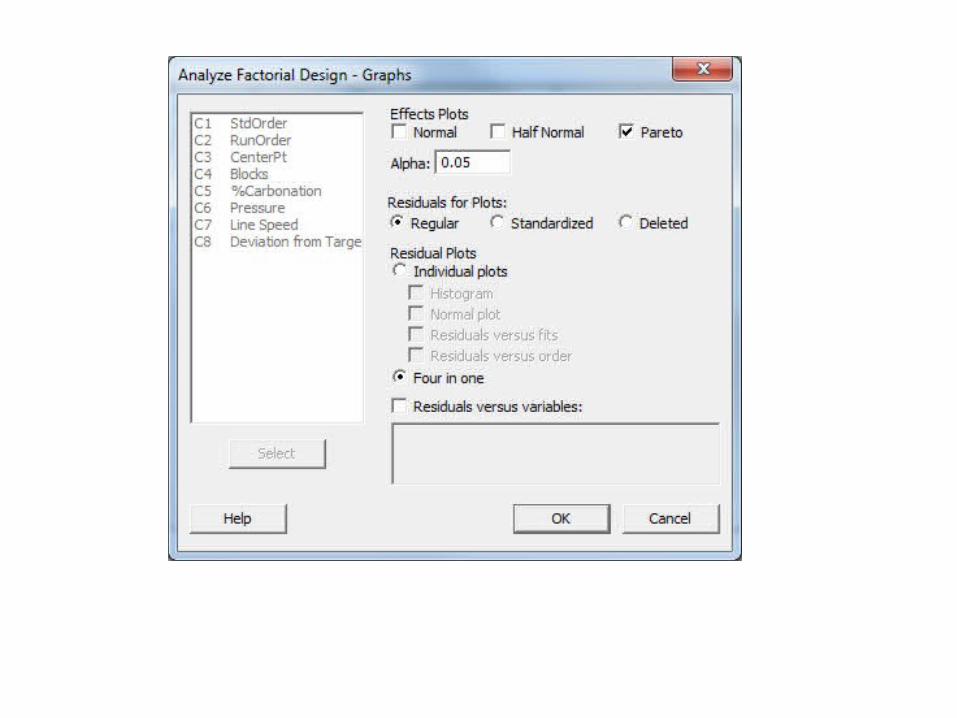
Select the Graphs tab to get the next screen

Select “Deviation”As Response

Term

Standardized Effect

AC

BC

ABC

AB

C

B

A

876543210

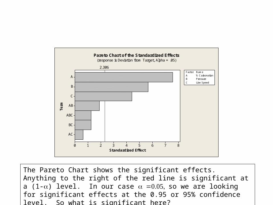
2.306Factor NameA % CarbonationB Pressure

C Line Speed

Pareto Chart of the Standardized Effects(response is Deviation from Target, Alpha = .05)

The Pareto Chart shows the significant effects. Anything to the right of the red line is significant at a (1-) level. In our case so we are looking for significant effects at the 0.95 or 95% confidence level. So what is significant here?

Residual

Perc

ent

10-1

99

90

50

10

1

Fitted Value

Resi

dual

6420-2

1.0

0.5

0.0

-0.5

-1.0

Residual

Fre

quency

1.00.50.0-0.5-1.0

6.0

4.5

3.0

1.5

0.0

Observation Order

Resi

dual

16151413121110987654321

1.0

0.5

0.0

-0.5

-1.0

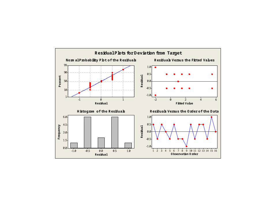
Normal Probability Plot of the Residuals Residuals Versus the Fitted Values

Histogram of the Residuals Residuals Versus the Order of the Data

Residual Plots for Deviation from Target

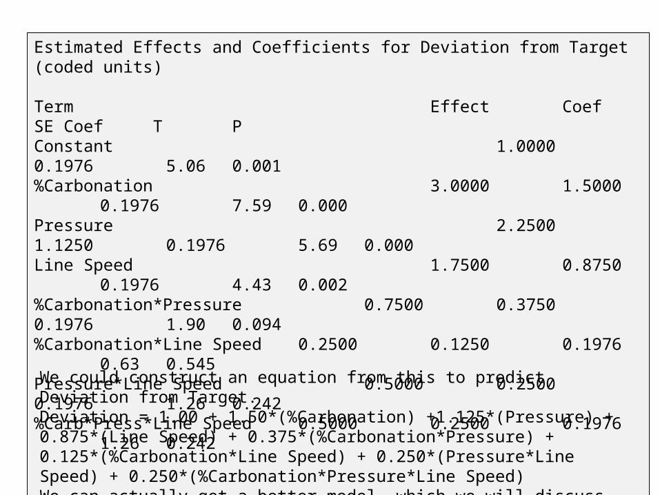
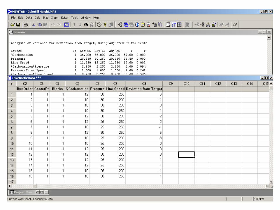
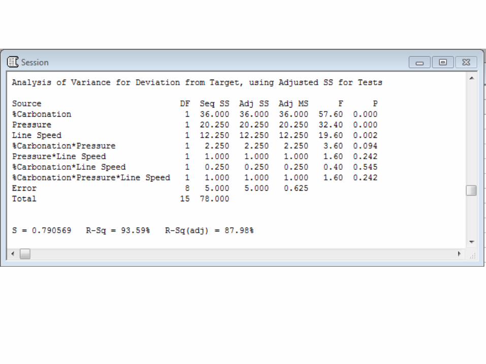
Estimated Effects and Coefficients for Deviation from Target (coded units)

Term Effect Coef SE Coef T PConstant 1.0000 0.1976 5.06 0.001%Carbonation 3.0000 1.5000 0.1976 7.59 0.000Pressure 2.2500 1.1250 0.1976 5.69 0.000Line Speed 1.7500 0.8750 0.1976 4.43 0.002%Carbonation*Pressure 0.7500 0.3750 0.1976 1.90 0.094%Carbonation*Line Speed 0.2500 0.1250 0.1976 0.63 0.545Pressure*Line Speed 0.5000 0.2500 0.1976 1.26 0.242%Carb*Press*Line Speed 0.5000 0.2500 0.1976 1.26 0.242

S = 0.790569 PRESS = 20R-Sq = 93.59% R-Sq(pred) = 74.36% R-Sq(adj) = 87.98%

We could construct an equation from this to predict Deviation from Target. Deviation = 1.00 + 1.50*(%Carbonation) +1.125*(Pressure) + 0.875*(Line Speed) + 0.375*(%Carbonation*Pressure) + 0.125*(%Carbonation*Line Speed) + 0.250*(Pressure*Line Speed) + 0.250*(%Carbonation*Pressure*Line Speed)We can actually get a better model, which we will discuss in a few slides.

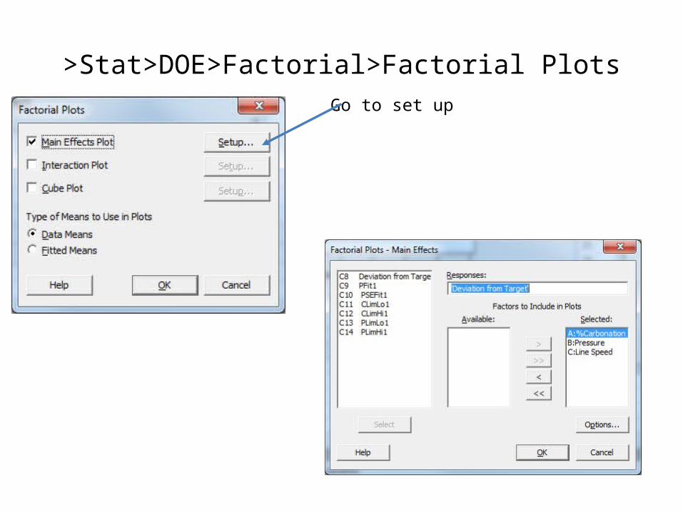
>Stat>DOE>Factorial>Factorial PlotsGo to set up

Mean o

f Devia

tion fro

m T

arg

et

1210

2

1

0

3025

250200

2

1

0

%Carbonation Pressure

Line Speed

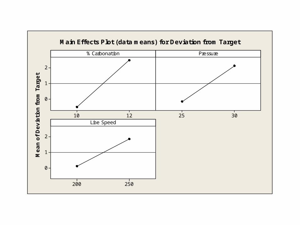
Main Effects Plot (data means) for Deviation from Target

Practical Application

Carbonation has a large effect, so try to control the temperature more precisely

There is less deviation at low pressure, so use the low pressure

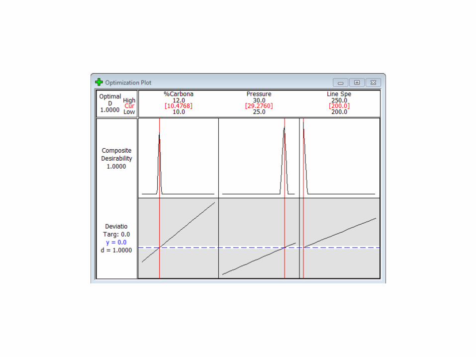
Although the slower line speed yields slightly less deviation, the process engineers decided to go ahead with the higher line speed - WHY???

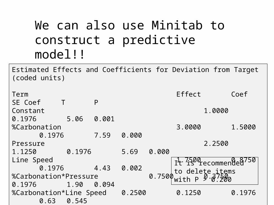
We can also use Minitab to construct a predictive model!!

Estimated Effects and Coefficients for Deviation from Target (coded units)

Term Effect Coef SE Coef T PConstant 1.0000 0.1976 5.06 0.001%Carbonation 3.0000 1.5000 0.1976 7.59 0.000Pressure 2.2500 1.1250 0.1976 5.69 0.000Line Speed 1.7500 0.8750 0.1976 4.43 0.002%Carbonation*Pressure 0.7500 0.3750 0.1976 1.90 0.094%Carbonation*Line Speed 0.2500 0.1250 0.1976 0.63 0.545Pressure*Line Speed 0.5000 0.2500 0.1976 1.26 0.242%Carb*Press*Line Speed 0.5000 0.2500 0.1976 1.26 0.242

S = 0.790569 PRESS = 20R-Sq = 93.59% R-Sq(pred) = 74.36% R-Sq(adj) = 87.98%

It is recommended to delete items with P > 0.200

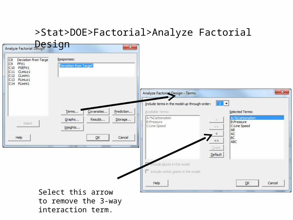
>Stat>DOE>Factorial>Analyze Factorial Design

Select this arrow to remove the 3-way interaction term.

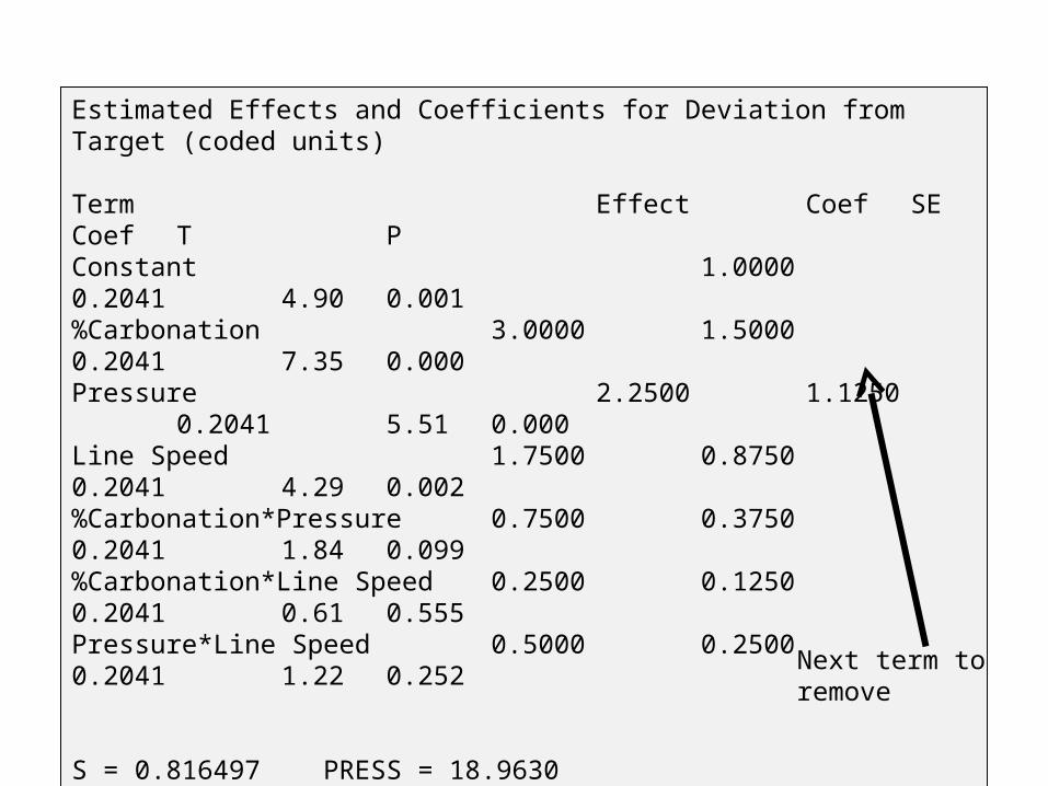
Estimated Effects and Coefficients for Deviation from Target (coded units)

Term Effect Coef SE Coef T PConstant 1.0000 0.2041 4.90 0.001%Carbonation 3.0000 1.5000 0.2041 7.35 0.000Pressure 2.2500 1.1250 0.2041 5.51 0.000Line Speed 1.7500 0.8750 0.2041 4.29 0.002%Carbonation*Pressure 0.7500 0.3750 0.2041 1.84 0.099%Carbonation*Line Speed 0.2500 0.1250 0.2041 0.61 0.555Pressure*Line Speed 0.5000 0.2500 0.2041 1.22 0.252

S = 0.816497 PRESS = 18.9630R-Sq = 92.31% R-Sq(pred) = 75.69% R-Sq(adj) = 87.18%

Next term to remove

Here is the final model from Minitab with the appropriate terms.

Estimated Effects and Coefficients for Deviation from Target (coded units)

Term Effect Coef SE Coef T PConstant 1.0000 0.2030 4.93 0.000%Carbonation 3.0000 1.5000 0.2030 7.39 0.000Pressure 2.2500 1.1250 0.2030 5.54 0.000Line Speed 1.7500 0.8750 0.2030 4.31 0.001%Carbon*Press 0.7500 0.3750 0.2030 1.85 0.092

S = 0.811844 PRESS = 15.3388R-Sq = 90.71% R-Sq(pred) = 80.33% R-Sq(adj) = 87.33%

Deviation from Target = 1.000 + 1.5*(%Carbonation) + 1.125*(Pressure) + 0.875*(Line Speed) + 0.375*(%Carbonation*Pressure)

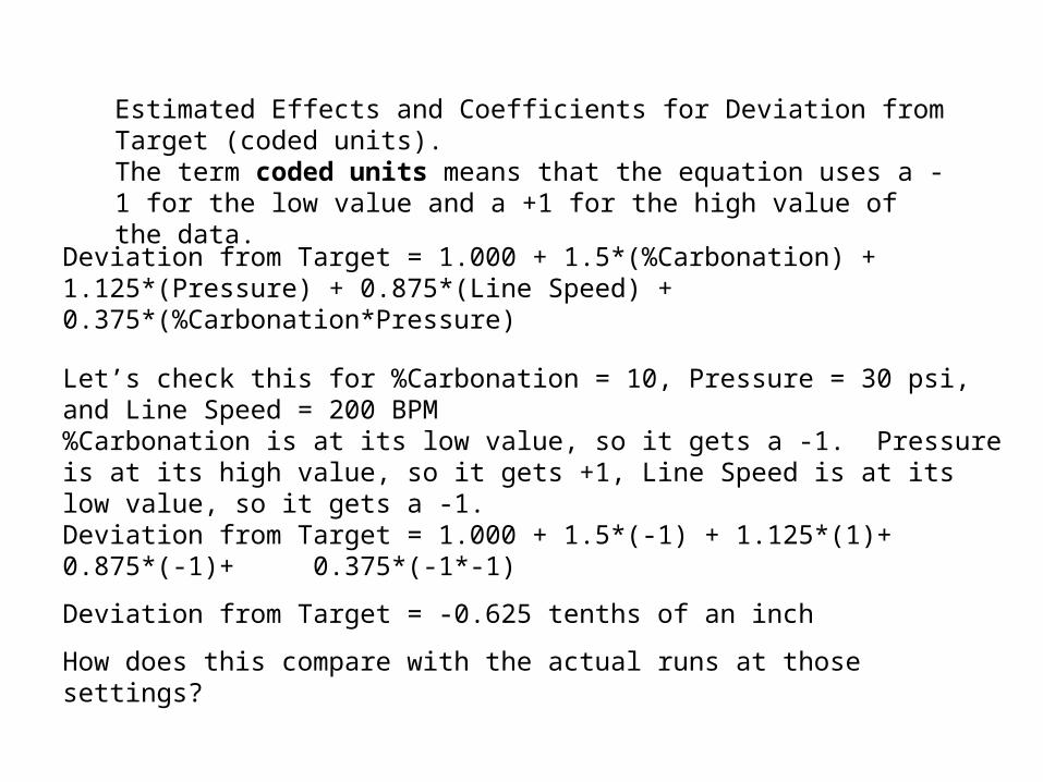
Estimated Effects and Coefficients for Deviation from Target (coded units).The term coded units means that the equation uses a -1 for the low value and a +1 for the high value of the data.

Deviation from Target = 1.000 + 1.5*(%Carbonation) + 1.125*(Pressure) + 0.875*(Line Speed) + 0.375*(%Carbonation*Pressure)

Let’s check this for %Carbonation = 10, Pressure = 30 psi, and Line Speed = 200 BPM%Carbonation is at its low value, so it gets a -1. Pressure is at its high value, so it gets +1, Line Speed is at its low value, so it gets a -1.

Deviation from Target = 1.000 + 1.5*(-1) + 1.125*(1)+ 0.875*(-1)+ 0.375*(-1*-1)

Deviation from Target = -0.625 tenths of an inch

How does this compare with the actual runs at those settings?

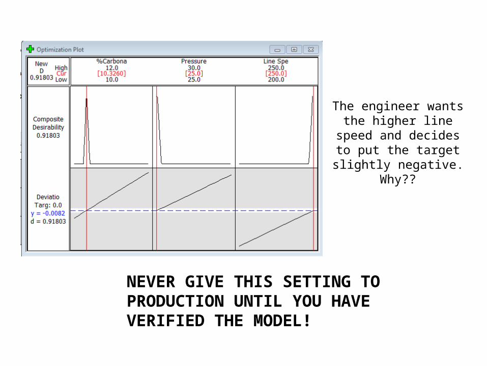
NEVER GIVE THIS SETTING TO PRODUCTION UNTIL YOU HAVE VERIFIED THE MODEL!

The engineer wants the higher line speed and

decides to put the target slightly negative. Why??

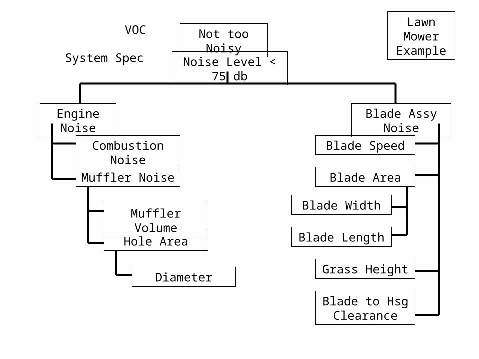
Not too Noisy

Noise Level < 75 db

VOC

System Spec

Lawn Mower

Example

Engine Noise Blade Assy Noise

Combustion Noise

Muffler Noise

Muffler Volume

Hole Area

Diameter

Blade Speed

Blade Area

Blade Width

Blade Length

Grass Height

Blade to Hsg Clearance