STATISTICS AND DATA INVESTIGATION AND INTERPRETATION …amsi.org.au/.../pdfs/Data_Investigation_and_interpretation5.pdf · DATA INVESTIGATION AND INTERPRETATION {4} A guide for teachers

$Page 1: STATISTICS AND DATA INVESTIGATION AND INTERPRETATION …amsi.org.au/.../pdfs/Data_Investigation_and_interpretation5.pdf · DATA INVESTIGATION AND INTERPRETATION {4} A guide for teachers$
5YEAR

DATA INVESTIGATION AND INTERPRETATIONThe Improving Mathematics Education in Schools (TIMES) Project

A guide for teachers - Year 5 June 2011

STATISTICS AND PROBABILITY Module 3

Data Investigation and Interpretation

(Statistics and Probability : Module 3)

For teachers of Primary and Secondary Mathematics

510

Cover design, Layout design and Typesetting by Claire Ho

The Improving Mathematics Education in Schools (TIMES)

Project 2009‑2011 was funded by the Australian Government

Department of Education, Employment and Workplace

Relations.

The views expressed here are those of the author and do not

necessarily represent the views of the Australian Government

Department of Education, Employment and Workplace Relations.

© The University of Melbourne on behalf of the International

Centre of Excellence for Education in Mathematics (ICE‑EM),

the education division of the Australian Mathematical Sciences

Institute (AMSI), 2010 (except where otherwise indicated). This

work is licensed under the Creative Commons Attribution‑

NonCommercial‑NoDerivs 3.0 Unported License.

http://creativecommons.org/licenses/by‑nc‑nd/3.0/

Helen MacGillivray

5YEAR

DATA INVESTIGATION AND INTERPRETATION

The Improving Mathematics Education in Schools (TIMES) Project

A guide for teachers - Year 5 June 2011

STATISTICS AND PROBABILITY Module 3

DATA INVESTIGATION AND INTERPRETATION

{4} A guide for teachers

ASSUMED BACKGROUND FROM F-4

It is assumed that in Years F‑4, students have had many learning experiences involving

choosing and identifying questions or issues from everyday life and familiar situations and

planning statistical investigations that involve data in which observations fall into natural or

assembled categories.

It is assumed that students have had learning experiences in recording, classifying and

exploring such data, and have seen and used tables, picture graphs and column graphs of

categorical data with natural or assembled categories.

It is assumed that some of these experiences involved count data with a small number of

different counts that were treated as categories.

MOTIVATION

Statistics and statistical thinking have become increasingly important in a society that

relies more and more on information and calls for evidence. Hence the need to develop

statistical skills and thinking across all levels of education has grown and is of core

importance in a century which will place even greater demands on society for statistical

capabilities throughout industry, government and education.

A natural environment for learning statistical thinking is through experiencing the process

of carrying out real statistical data investigations from first thoughts, through planning,

collecting and exploring data, to reporting on its features. Statistical data investigations

also provide ideal conditions for active learning, hands‑on experience and problem‑

solving.

Real statistical data investigations involve a number of components: formulating a

problem so that it can be tackled statistically; planning, collecting, organising and

validating data; exploring and analysing data; and interpreting and presenting information

from data in context. A number of expressions to summarise the statistical data

investigative process have been developed but all provide a practical framework for

demonstrating and learning statistical thinking. One description is Problem, Plan, Data,

Analysis, Conclusion (PPDAC); another is Plan, Collect, Process, Discuss (PCPD).

No matter how it is described, the elements of the statistical data investigation process are

accessible across all educational levels.

{5}The Improving Mathematics Education in Schools (TIMES) Project

CONTENT

In this module, in the context of statistical data investigations, we introduce measurement

data. We contrast measurement data with categorical data and count data, and also

consider more general examples of count data than in the Year 4 module.

Some examples of measurement data are:

• time in minutes to eat lunch

• length in cm of right feet of Year 5 girls

• age in years

• weight in kg of Year 5 boys

All measurement data need units of measurement and observations are recorded in the

desired units of measurement.

In categorical data each observation falls into one of a number of distinct categories.

Such data are everywhere in everyday life. Some examples are:

• gender

• direction on a road

• type of dwelling

Sometimes the categories are natural, such as with gender or direction on a road, and

sometimes they require choice and careful description, such as type of dwelling.

Each observation in a set of count data is a count value. Count data occur in considering

situations such as:

• the number of children in a family

• the number of children arriving at the tuckshop in a 5 minute interval

• the number of vehicles passing in 2 minutes


This module uses a number of examples to illustrate these different types of data and to

develop the statistical data investigation process through the following:

• considering initial questions that motivate an investigation;

• identifying types of data that could be involved in investigating the questions;

• identifying issues and planning;

• collecting, handling and checking data;

• exploring and interpreting data in context.

Such phases lend themselves to representation on a diagram, as follows.

Collecting, handling,

checking data

Initial questions

Exploring, interpreting data in context

Issues and planning

Types of data involved

The examples consider situations familiar and accessible to Year 5 students, and build on

the situations considered in F‑ 4.

INITIAL QUESTIONS THAT CAN MOTIVATE AN INVESTIGATION.

The following are some examples of questions that involve collecting and investigating

measurement, categorical or count data.

A How long does it take you to get to school in the morning?

B How tall are you? What is the length of your arm span from fingertip to fingertip when

you stretch your arms out sideways? What is the difference between your span and

your height? How does it compare with others in your class?

C For how long can you balance a book on your head? How do you compare with

others in your class? How much does it vary when you do it lots of times?

D How many shots are there in a tennis game before each point is won? How much

do they vary over a whole match?

E How much time is there between shots at goal in a football (soccer) match?

How much variation is there over a match?


F How many passes are there in a football or netball match? How much does this

number vary over matches?

G How many vehicles go past your school every 2 minutes?

H How many different types of trees are there in your school’s neighbourhood?

How would you classify them? How many trees are there of each type in the

playing fields of your school or in a local park?

I How many times does the word ‘Harry’ appear per page in a Harry Potter book?

How much does this vary over pages?

J How many different types of letterboxes are there in your neighbourhood?

How would you classify them? How many letterboxes of each type are there

in your neighbourhood?

The above are examples of just some of the many questions that can arise that involve

measurement, count or categorical data. Some of these questions are used here

to explore the progression of development of learning about data investigation and

interpretation. The focus in this module in exploring and interpreting is on one dataset

at a time; for example, in Example B, data on height and span would be explored

separately to each other.

MEASUREMENT, CATEGORICAL AND COUNT DATA

Before considering issues and planning, collecting, exploring and interpreting data with

some of the above examples, the types of data are considered for all the examples. Also

considered below are the general types of subjects – that is, on or from what will the

observations be collected or observed.

A The times for different students to get to school are measurement data.

The observations are taken for each selected student.

B The heights and spans of students are measurement data. There are two measurement

variables, height and span, and from these can be calculated another, span‑height. The

observations are taken for each selected student.

C How long different students can balance a book on their heads are measurement data.

The observations are for each student. Repeatedly measuring how long one student

can balance a book on his or her head gives a different type of set of measurement

data in which the observations are taken for each attempt for that student.

D Recording the number of shots before each point is won in a tennis match gives a set

of count data. For each point we count the number of shots until the point is won. The

observations are observed for each point.

E Recording the times between shots at goal in a football (soccer) match gives a set of

measurement data. The observations are observed for each shot at goal.

F Recording the number of passes in a series of football or netball matches gives a set of

count data. The observations are collected for each match.


G Recording the numbers of cars passing in 2 minutes over a number of 2 minute

intervals gives a set of count data. The observations are collected for each 2 minutes.

H Type of tree is categorical. Classifying the trees in a region into types gives a set of

categorical data. The observations are taken for each tree sampled.

I Recording the number of times the word ‘Harry’ appears on a sample of pages from

a Harry Potter book gives a set of count data. The observations are recorded for each

selected page.

J Type of letterbox is categorical. Classifying the letterboxes in your neighbourhood into

types gives a set of categorical data. The observations are per type.

General statistical notes for teachers

Types of data – types of variables

When we collect or observe data, the ‘what’ we are going to observe is called a statistical

variable. You can think of a statistical variable as a description of an entity that is being

observed or is going to be observed. Hence when we consider types of data, we are also

considering types of variables.

Measurement variables are examples of continuous variables; continuous variables

can take any values in intervals. More about continuous variables is seen in Years 7 and

upwards. Measurement data have units of measurement and are recorded with a certain

precision that depends on the measuring instrument, the choice of the investigator and

practical restrictions.

A categorical variable takes names or values that represent distinct categories. The

categories are usually natural categories such as cat or dog, male or female, but often

there are many possible categories or different possible descriptions. If so, we need to

carefully choose our groupings and descriptions of them.

A count variable counts the number of items or people in a specified time or place or

occasion or group.

IDENTIFYING ISSUES AND PLANNING

In the first part of the data investigative process, one or more questions or issues begin

the process of identifying the topic to be investigated. In thinking about how to investigate

these, other questions and ideas can tend to arise. Refining and sorting these questions

and ideas along with considering how we are going to obtain data that is needed to

investigate them, help our planning to take shape. A data investigation is planned through

the interaction of the questions:

• ‘What do we want to find out about?’

• ‘What data can we get?’ and

• ‘How do we get the data?’


EXAMPLE B: HEIGHTS AND SPANS

The general topic is investigating heights and spans and their difference in Year 5 students.

What are possible issues of interest? Both the sizes and the variation of heights and spans

across the class are of interest. Why would we be interested in the difference of span‑

height? Again both the general sizes and variation of the differences are of interest. Perhaps

the students can think of other reasons, for example, to do with manufacture of clothing.

There are two measurements to be made on each student. Heights should be measured

without shoes. The same way of measuring heights and spans should be followed

carefully. There may be guidelines given on the web for measuring height. Why would this

be so? Perhaps because height is such an important variable in monitoring growth. Would

there be as much interest in span? If not, why not?

An example of how heights were used in the past in relation to ages of children can be

found at http://old.rsscse.org.uk/qca/resource6.htm

EXAMPLE D: NUMBER OF SHOTS IN POINTS IN TENNIS

There is always at least one shot with the first serve. So if the first serve is in and is an ace,

there is just one shot. If a serve is a fault, do we count it as one of the shots of the point?

It does not lead to a rally but it is a shot in the point. What we decide to do depends to

some extent on the reason for our interest. Are we investigating length of rallies or are we

interested in the numbers of shots from the point of view of the amount of effort needed

in tennis? If we do not count faults and lets, then it is possible to have observations of

zero. If we do count total number of shots then we include faults and lets.

There can be many shots in a rally before the point is won. We would need to decide if

we are interested in top players’ matches or in matches played by students learning to

play tennis. We could collect a dataset for just one match or even one set of a match, or

we could collect our data by recording the number of shots in points chosen at random.

Different students or groups of students could choose different matches or parts of

matches to record the numbers of shots.

If we choose to look at top players’ matches, do we look at men’s or women’s matches?

Although in some tournaments, men play best of 5 and women best of 3, the number of

points can vary considerably over both men’s and women’s matches, so students could

choose a match they would like to investigate and compare their data with others.


EXAMPLE E: TIME BETWEEN SHOTS AT GOAL IN SOCCER

As with the tennis example, students’ interest may be in top level soccer such as Australian

A league or the English Premier League or in matches played in their age group or an

older age group. Unlike the tennis example, and because the variable is time between

shots at goal, focus will tend to be on data collected for a match. As with the tennis

example, different students or groups of students could choose different matches and

compare their datasets.

An important point here is to decide what is a shot at goal and to describe this carefully so

that different students/groups of students collect data with a consistent definition of shot

at goal. Because number of shots at goal is one of the summary statistics that is quoted

for soccer matches, some guidelines on defining a shot at goal should be available, or

possibly are already known by students who have started playing soccer.

EXAMPLE I: COUNT OF THE WORD ‘HARRY’ PER PAGE

The interest in this example is not only how often the word ‘Harry’ tends to appear per

page of a Harry Potter book, but also on how variable this is across pages. A practicality

is to decide whether to count words such as ‘Harry’s’. It is most unlikely that a word like

Harry would be hyphenated or apostrophised across pages but if students do find this on

any selected pages, they would seek guidance.

EXAMPLE J: TYPES OF LETTERBOXES

As with much categorical data, an issue in planning in this example is choosing and

carefully describing the categories. For example, letterboxes could be classified by type

of material, size, elaborateness etc. If material, they could be classified by their major

material, for example, brick, wood, metal, other.

Another aspect for discussion or selection by the teacher is choice of region. This point is

taken up below.


COLLECTING, HANDLING AND CHECKING DATA

EXAMPLE B: HEIGHTS, SPANS AND DIFFERENCES FOR YEAR 5 STUDENTS

Apart from everyone being measured in the same way with shoes off, the only other

questions in relation to collecting these data relate to desired precision of measurement.

For example, is the same tape measure to be used? Should the same person take all the

measurements? Should we measure to the nearest cm or to the nearest 0.5cm? For usual

values of height and span for Year 5 students, the extra precision obtained through using

the same tape measure and same person to measure may be unnecessary. Because the

values of the differences (span‑height) are not familiar, reasonable care may be needed

to obtain accurate measurements of these, but the variation is likely to swamp minor

inconsistencies in measurements.

The recording sheet is simple and the first few rows would look like the following.

STUDENT NAME

HEIGHT IN CM

SPAN IN CM

SPAN – HEIGHT IN CM

Abigail 136.5 cm 135.5 cm –1 cm

Fred 132 cm 134.5 cm 2.5 cm

Jenny 134.5 cm 136 cm 1.5 cm

EXAMPLE D: NUMBER OF SHOTS TO WIN A POINT IN TENNIS

If it is decided to collect the data for all the points in a match or a set, then the data

collection is simply a matter of accuracy and reporting which match/set. As this data

collection is in real time, it is advisable for at least pairs of students to work together.

It is likely and probably easier to manage that students at this level will prefer to focus on a

set or a match. They may ask how many points they should observe, and may think they

need to observe the same number of points if different datasets are to be collected. This is

not necessary, and observing all of a set with differing number of points could add to the

interest in exploring the data.

If it is decided to choose points from across sets or even across matches, how to choose

them at random is not necessarily straightforward. Use of random numbers by the teacher

would be required, but as instructions based on any sequence produced is likely to cause

confusion at this level, it may be best simply to allow students to choose in a way they

think is ‘random’.


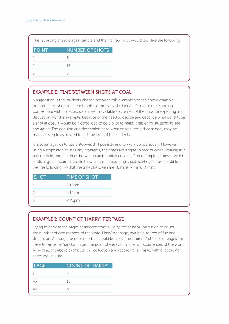
The recording sheet is again simple and the first few rows would look like the following.

POINT NUMBER OF SHOTS

1 3

2 12

3 5

EXAMPLE E: TIME BETWEEN SHOTS AT GOAL

A suggestion is that students choose between this example and the above example

on number of shots in a tennis point, or possibly similar data from another sporting

context, but with collected data in each available to the rest of the class for exploring and

discussion. For this example, because of the need to decide and describe what constitutes

a shot at goal, it would be a good idea to do a pilot to make it easier for students to see

and agree. The decision and description as to what constitutes a shot at goal, may be

made as simple as desired to suit the level of the students.

It is advantageous to use a stopwatch if possible and to work cooperatively. However if

using a stopwatch causes any problems, the times are simple to record when working in a

pair or triple, and the times between can be obtained later. If recording the times at which

shots at goal occurred, the first few lines of a recording sheet, starting at 2pm could look

like the following. So that the times between are 10 mins, 2 mins, 8 mins.

SHOT TIME OF SHOT

1 2.10pm

2 2.12pm

3 2.20pm

EXAMPLE I: COUNT OF ‘HARRY’ PER PAGE

Trying to choose the pages at random from a Harry Potter book, on which to count

the number of occurrences of the word ‘Harry’ per page, can be a source of fun and

discussion. Although random numbers could be used, the students’ choices of pages are

likely to be just as ‘random’ from the point of view of number of occurrences of the word.

As with all the above examples, the collection and recording is simple, with a recording

sheet looking like:

PAGE COUNT OF ‘HARRY’

5 7

43 15

49 5



The choice of region and organisation of collecting these data needs to be managed

for safety reasons, avoiding of doubling‑up of recording, and to obtain consistency in

categorisation. Once students have decided and described their classifications of letterboxes,

a small pilot will help in consistent classification. A recording sheet could look like:

LETTERBOX TYPE

2, Pumpkin Ct wood

4, Pumpkin Ct metal

6, Pumpkin Ct brick


Each of the above examples demonstrates how planning a statistical investigation involves

identification of the variables to be observed (what data are we going to collect) and the

‘subjects’ or ‘experimental units’ of the investigation – that is, on what we are going to

collect or observe our variables?

But these examples also naturally introduce early notions of the question: of what are our

data representative? With respect to heights, is our class representative of Australian Year

5’s? Of this age group 200 years ago? Of this age group in other countries? Is the tennis

match or soccer match we chose representative of matches at that level? Is the region in

which we looked at letterboxes representative of the city or a larger region?

EXPLORING AND INTERPRETING DATA

It is in exploring data that we use presentations, including graphical and summary

presentations.

Categorical data are summarised by the number of observations that fall in each category.

These are called the frequencies of the data – how often did each category occur. These

frequencies can be presented in a table or can be graphed by a column graph in which

each category has a column and the heights of the columns represent the frequency of

the observations that fall in that category. Column graphs are also called barcharts.

Count data are also summarised by the number of observations that fall in each

category, where the categories correspond to the different possible count values that

the observations take. If most observations are for only a few different counts, but there

are also a few large or unusual counts, these are sometimes grouped together in a

category and the count data are treated as categorical (See examples in the module,

Data Investigation and Interpretation – Year 4)

Frequencies of categories or of count values are the numbers of observations in the data

that fall into each category or that take each count value. It is frequencies that provide

the information on how likely are the different categories or count values – which tend to

occur more frequently and which tend to occur less frequently.


Measurement data can be presented by dotplots. A dotplot plots quantitative data, with

a dot on the graph for each value in the set of quantitative data. If a value occurs 3 times,

there are 3 dots in a line above that value. Hence the heights of the columns of dots give

the frequencies of the data values. If there are many observations in the dataset, each dot

might represent two or three observations. For measurement data, a dotplot is a plot of

the ‘raw’ data with no grouping of values. So if a set of measurement values is not large

and has many different values, a dotplot is not very informative, but a dotplot is usually an

excellent way to have a first look at data. Count data can also be represented by a dotplot.

Dotplots are easily done by hand and are also available in most statistical software.


Measurement data are observed in units of measurement and are recorded correct to

some unit of measurement. In this module, we just see simple plots of frequencies of the

different values observed in the data, but in later modules we see that measurement data

values are actually small intervals. For example, ‘the boy has a height of 140cm’ is more

correctly said as ‘the boy has a height between 139.5 and 140.5 cm’

EXAMPLE B: HEIGHTS, SPANS AND SPAN-HEIGHT

Below are some dotplots of height, span and span‑height (all in cm) for 30 Year 5

students. The dotplots show that both the heights and the spans vary from about 120 cm

to 146cm in height and 148 cm in span. So these plots indicate that the spans and heights

may be close to similar. The dotplot of span‑height shows that students’ spans vary from

3cm less than height up to 6 cm more than their height, with more students having their

spans slightly greater than their heights.

120 124 128 132 136 140 144

0 2 4 6

120 124 128 132 136 140 144 148

Dotplot of height in cm

height

span

Dotplot of span in cm

Dotplot of span-height in cm

span-height


EXAMPLE D: NUMBER OF SHOTS TO WIN A POINT IN TENNIS

Below is a dotplot of the number of shots in each point in a set of tennis. We see that

there were 6 points that were won with an ace on the first serve, and that even more

points were won with just two shots – so either a fault and then an ace or a first serve in

and then a winning return. If the number of shots went beyond two, there tended to be at

least a few more shots, and in some cases many more, before the point ended.

1 3 6 9 12 15 18 21

number of shots

Dotplot of number of shots in tennis point

EXAMPLE E: TIME BETWEEN SHOTS AT GOAL IN SOCCER

Below is a dotplot of the time in minutes between shots at goal in a soccer match.

Because the times are rounded to the nearest minute, there are 4 that have been rounded

to 0 – these were probably ‘second’ or ‘third’ rebound shots within the goal square. There

are quite a few low times and a small number of greater times with one of 15 minutes.

0 2 4 6 8 10 12 14

time between

Dotplot of time in minutes between shots at goal in a soccer match

EXAMPLE I: NUMBER OF HARRYS PER PAGE

Below is a dotplot of the numbers of Harrys per page from 100 pages chosen randomly

from a Harry Potter book. Most of the pages have low numbers of Harrys, but, like the

datasets above on numbers of shots in tennis points and time between shots at goal in

soccer, there are some pages with 6 to 12 occurrences of the word ‘Harry’.

0 2 4 6 8 10 12

No. of Harrys

Dotplot of number of Harrys per page



This is categorical data so a column graph is the appropriate graph. Below is a column

graph of 27 letterboxes classified by their main material. Brick was the most common

material, with metal and wood occurring in similar frequencies to each other.

GRAPH OF TYPE OF LETTERBOX

FRE

QU

EN

CY

TYPE OF LETTERBOX

8

10

12

6

4

2

brick metal wood0

SOME GENERAL COMMENTS AND LINKS FROM F-4 AND TOWARDS YEAR 6

As in Year 4, although the focus is on considering just one variable at a time, the above

examples again illustrate the extent of statistical thinking involved in the initial stages of an

investigation in identifying the questions/issues and in planning and collecting the data.

The above examples also show that at least some indications of concepts of ‘what do our

data represent’ and variation in data across samples, tend to arise naturally in everyday

situations that are very familiar to young students.

The examples here focus on a measurement, count or categorical variable and consider

two types of graphs. Measurement variables are continuous variables (they take values

in intervals); count and categorical variables are discrete variables (they take separated

values). The word ‘continuous’ should be used as students progress to the higher years.

Dotplots are for quantitative data and column graphs are for categorical data. Both types

of graphs show the frequencies of the different values in the dataset, but the distances

between ticks along the x‑axis in a dotplot are quantitative and meaningful, whereas

the arrangement of categories along the x‑axis in a column graph is arbitrary and the

distances between the columns have no meaning. Column graphs are sometimes used

for count data with only a few different values, but usually to use column graphs for count

data, the count data need to be converted to categorical data with the last category being


‘more than …’. The examples above show how information can be lost in many situations

by such grouping.

Although some of the examples in Year 5 involve more than one variable and the

motivating questions do in fact include, or teeter on including, comparisons of data for

one variable across categories of another categorical variable, such comparisons have

been only lightly touched on. In Year 6 we restrict attention again to categorical variables,

but start considering the possibility of association between variables. Does the behaviour

of one of the variables depend on the other?

www.amsi.org.au

The aim of the International Centre of Excellence for

Education in Mathematics (ICE‑EM) is to strengthen

education in the mathematical sciences at all levels‑

from school to advanced research and contemporary

applications in industry and commerce.

ICE‑EM is the education division of the Australian

Mathematical Sciences Institute, a consortium of

27 university mathematics departments, CSIRO

Mathematical and Information Sciences, the Australian

Bureau of Statistics, the Australian Mathematical Society

and the Australian Mathematics Trust.

The ICE‑EM modules are part of The Improving

Mathematics Education in Schools (TIMES) Project.

The modules are organised under the strand

titles of the Australian Curriculum:

• Number and Algebra

• Measurement and Geometry

• Statistics and Probability

The modules are written for teachers. Each module

contains a discussion of a component of the

mathematics curriculum up to the end of Year 10.

Documents

STATISTICS AND DATA INVESTIGATION AND INTERPRETATION …amsi.org.au/.../pdfs/Data_Investigation_and_interpretation5.pdf · DATA INVESTIGATION AND INTERPRETATION {4} A guide for teachers