+

I

Statistics and Data Analysis in Geology Third Edition

John C. Davis Kansas Geological Survey The University of Kansas

~~ 'WILEY INDIA

Statistics and Data Analysis in Geology- Chapter 5

treated as though they occurred along a single, straight sampling line. This and other methods for investigating the density of patterns of lines are reviewed by Getis and Boots (1978). A computer program for computing nearest-neighbor dis­tances, orientation, and other statistical measures of patterns of lines is given by Clark and Wilson (1994).

Analysis of Directional Data Directional data are an important category of geologic information. Bedding planes fault surfaces, and joints are all characterized by their attitudes, expressed a~ strikes and dips. Glacial striations, sole marks, fossil shells, and water-laid peb­bles may have preferred orientations. Aerial and satellite photographs may show · oriented linear patterns. These features can be measured and treated quantitattvely like measurements of other geologic properties, but it is necessary to use special statistics that reflect the circular (or spherical) nature of directional data.

Following the practice of geographers, we can distinguish between direction~l and oriented features. Suppose a car is traveling north along a highway; the car's · motion has direction, while the highway itself has only a north-south orientation; Strikes of outcrops and the traces of faults are examples of geologic observations . that are oriented, while drumlins and certain fossils such as high-spired gastropods have clear directional characteristics.

We may also distinguish observations that are distributed on a circle, such as paleocurrent measurements, and those that are distributed spherically, such'as measurements of metamorphic fabric. The former data are conventionally shoWn as rose diagrams, a form of circular histogram,· while the latter are plotte!;l as points on a projection of a hemisphere. Although geologists have plotted diretl· tional measurements in these forms for many years, they have not used forinal. statistical techniques extensively to test the veracity of the conclusions they have drawn from their diagrams. This is doubly unfortunate; not only are these statis· tic:al tests useful, but the development of many of the procedures was origin.ally inspired by problems in the Earth sciences. · ' '

Figure 5-13 is a map of glacial striations measured in a small area of south· ern Finland; the measurements are listed in Table 5-4 and contained in file FIN· LAND.TXT. The directions indicated by the striations can be expressed by plottin& them as unit vectors or on a circle of unit radius as in Figure 5-14 a. If the circle is. subdivided into segments and the number of vectors within each segment counted, the results can be expressed as the rose diagram, or circular histogram, shown as Figure 5-14 b.

Nemec (1988) pointed out that many of the rose diagrams published by ge­ologists violate the basic principal on which histograms are based and, as a con· sequence, the diagrams are visually misleading. Recall that areas of columns in a histogram are proportional to the number (or percentage) of observations occurring in the corresponding intervals. For a rose diagram to correctly represent a circular distribution, it must be constructed so that the areas of the wedges (or "petals") of · the diagram are proportional to class frequencies. Unfortunately, most rose dia· grams are drawn so that the radii of the wedges are proportional to frequency. The resulting distortion may suggest the presence of a strong directional trend where none exists (Fig. 5-15). · ..

~pat1al Ana1ys1s

~ ~ ~~

~'::t...l~ ~ ~

~''::to..

'~ ' r

' ~ ~

~ ~

't ~f' ~ ~

I ~ ~

~ # I

' ~~

'::to..~ .,.,.

~ ;r

~ ~ ~ ~ ~

Figure 5-13. Map showing location and direction of 51 measurements of glacial striations in a 35-km2 area of southern Finland.

Table 5-4. Vector directions of ~lacial striations measured in an area of southern ~mland; measure-

ments given in degrees clockw1se from north .

23 105 127 144 171

27 113 127 145 172

53 113 128 145 179

58 114 128 146 181

64 117 129 153 186

83 121 132 155 190

85 123 132 155 212

88 125 132 155

93 126 134 157

99 126 135 163

100 126 137 165

If we define a radius for a sector of a rose diagram that represents either one observation, or 1%, we can easily calculate t~e appropriate radii that represent any number of observations or relative frequencres,

lrf (5.38) rf = ruw

where r is the unit radius representing one observation or 1%: f is the ~requency in co~s or ercent) of observations within a class, and rf IS the radius of the

. ~lass sector. ~other words, the radius shoul~ be proportional to the square root of the frequency rather than to the frequency Itself.

Rose diagrams, even if properly scaled, suffer fro~ ~he same prob~ems as or­din histograms; their appearance is ext~emel~ s.ensitl~e ~o the chmce. of class wid~ and starting point and they exhibit variations similar to the histogram

317

Statistics and Data Analysis in Geology- Chapter 5

270°

oo 360°

oo 360°

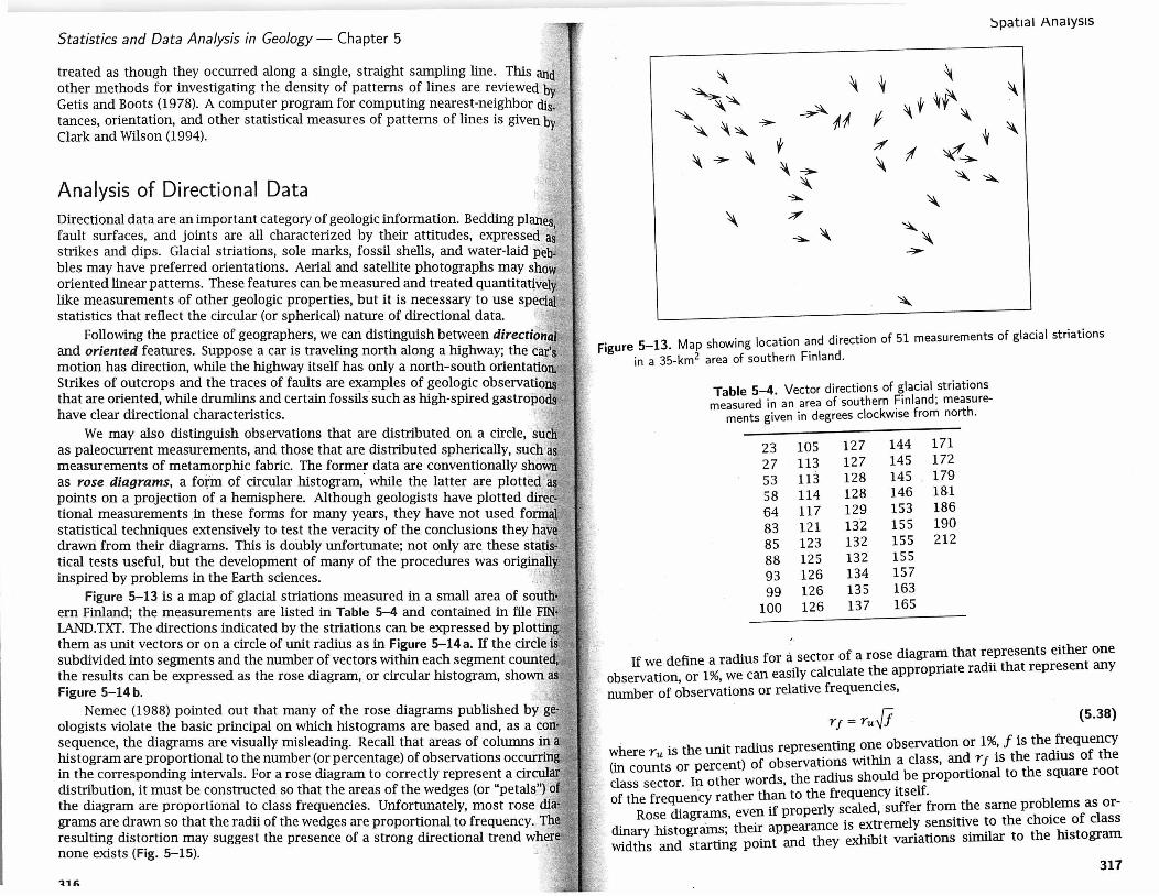
Figure 5-14. Directions of glacial striations shown on Figure 5-13. (a) Directions plotted as unit vectors. (b) Directions plotted as a rose diagram showing numbers of vectors within successive ).0° segments. ·

a b

Figure 5-15. Rose diagram of glacial striations shown on Figure 5-13 plotted in lOo seg­ments. (a) Length of petals proportional to frequency. (b) Area of petals proportional to frequency.

examples shown in Figure 2-11 on p. 30. Wells (1999) provides a computer program that quickly constructs rose diagrams with different conventions and also includes an assortment of graphical alternatives that may be superior to conventional rose diagrams for some uses (Fig. 5-16).

To compute statistics that describe characteristics of an entire set of vectors, we must work directly with the individual directional measurements rather than with a graphical summary such as a rose diagram. (Note that the following dis• · cussion uses geological and geographic conventions in which angles are measured clockwise from north, or from the positive end of the Y-axis. Many papers on di­rectional statistics follow a mathematical convention in which angles are measured' counterclockwise from east, or from the positive end of the X-axis.) ~

Spatial Analysis

a b c

d e f

Figure 5-16. Effect of choice of segment size and origin on appearance of rose diagrams. Data are directions of glacial striations from file FINLAND.TXT: (a) so segments, oo origin, outer ring 20%; (b) 15o segments, 0° origin, outer ring 30%; (c) 30o segments, oo origin, outer ring 40%; (d) 15° segments, 10° origin-compare to (b) . Alternative graphical forms include (e) kite diagram, 15° segments, oo origin-sometimes used in statistical presentations; (f) circular histogram, 15° segments, 0° origin-widely used to plot wind directions.

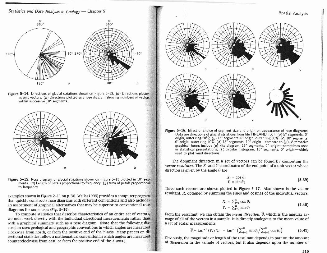
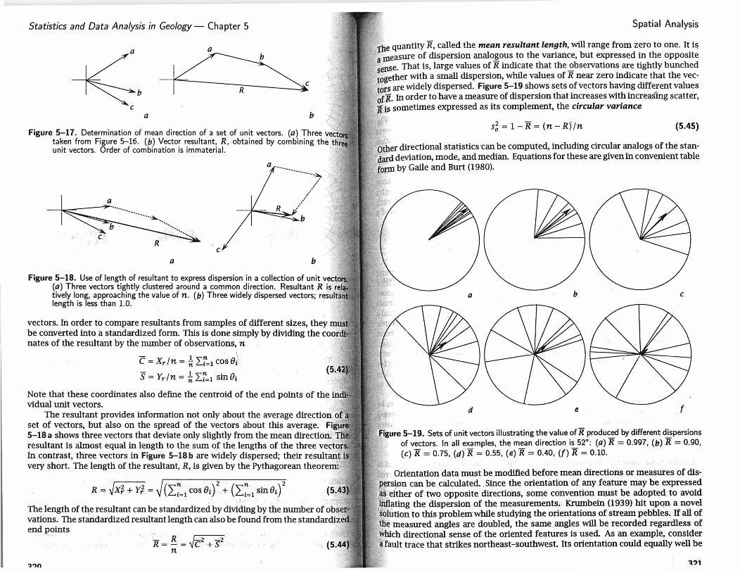
The dominant direction in a set of vectors can be found by computing the vector resultant. The X- andY-coordinates of the end point of a unit vector whose direction is given by the angle e are

xi= cos ei rt = sinei (5.39)

Three such vectors are shown plotted in Figure 5-17. Also shown is the vector resultant, R, obtained by summing the sines and cosines of the individual vectors:

Xr = L:r=l cos ei Yr = L:f= 1 sin ei

(5.40)

From the resultant, we can obtain the mean direction, 8, which is the angular av­erage of all of the vectors in a sample. It is directly analogous to the mean value of a set of scalar measurements

- -1 -1 ('n . /'n ) e =tan (Yr!Xr) =tan Li=l smei Li=l cos ei (5.41)

Obviously, the magrlitude or length of the resultant depends in part on the amount of dispersion in the sample of vectors, but it also depends upon the number of

319

Statistics and Data Analysis in Geology- Chapter 5

b I~ a b

Figure 5-17. Dete~mination of mean direction of a set of unit vectors. (a) Three taken from F1gure 5-16. (b) Vector resultant, R, obtained by combining the thri~ot•t• unit vectors. Order of combination is immaterial.

a ----------------'.)o.,

-------------. .

c a b

Figure 5-18. Use of length of resultant to express dispersion in a collection of unit (a) Three vectors tightly clustered around a common direction. Resultant R is tively long, approaching the value of n . (b) Three widely disperSed vectors· length is less than 1.0. · '

vectors. In order to compare resultants from samples of different sizes, they be converted into a standardized form. This is done simply by dividing the ""'''~'~'~''-" nates of the resultant by the number of observations, n ·

- 1 n \ c = Xrln = n Li=l cos 8i' - 1 n . . s = Yrln = n Li=1 smei

Note that these coordinates also define the centroid of the end points of the vidual unit vectors.

The resultant provides information not only about the average direction set of vectors, but also on the spread of the vectors about this a:verage. 5-18a shows three vectors that deviate only slightly from the mean direction: resultant is almost equal in length to the sum of the lengths of the three vec:rors.:.; In contrast, three vectors in Figure 5-18 b are Widely dispersed; their resultant very short. The length of the resultant, R, is given by the Pythagorean theorem:

.R = ~x; + Yi = ~ (I~=l co!! ei }2

+ (I:1 sin ei) 2

; '

The length of the resultant can be standardized by dividing by the number of vations. The standardized resultant length can also be found from the end J?Oints

:._ R ~-2 -2 R=-. = C +S

n j,

Spatial Analysis

'fbe quantity R, called the mean resultant. length, will range from zero to one. It i!! a measure of dispersion analo~ous to the variance, but expressed in the opposite sense. That is, large values of R indicate that the ~bservations are tightly bunched together with a small dispersion, while values of R near zero indicate that the vec­tors are widely dispersed. Figure 5-19 shows sets of vectors having different values ofR. In order to have a measure of dispersion that increases with increaslng scatter, JUs sometimes expressed as its complement, the circular variance

s~ = 1-R = (n- R)fn (5.45)

J; j; other directional statistics ·can be computed, including circular analogs of the stan-dard deviation, mode, and median. Equations for these are given in convenient table fof,rn by Gaile and Burt (1980).

c

d e f l t>l

Figure 5-19. Sets of unit vectors illustrating the value ofR produced by different dispersions of vectors. In all examples, the mean direction is 52°: (a) R = 0.997, (b) R = 0.90, (c) R = 0.75, (d) R = 0.55, (e) R = 0.40, (f) R = 0.10.

'' ' Orientation data must be modified before mean directions or measures of dis­

pers~~m can be calculated . . Since the orientation of any feature· may be expressed as. either of two opposite directions, some convention must be adopted. to avoid IJUI~ting the dispersion of the measurements. Krumbein (1939) hit upqn a novel soJution to this problem while studying the orientations of stream pebbles. If all of the measured angles are doubled, the same _angles will be recorded regardless of which directional sense of the oriented features is used. As an example, consider a fault trace that strikes northeast -southwest. Its orientation could equally well be

~?1

Statistics and Data Analysis in Geology- Chapter 5

recorded as 45 • or as 225 · . If we double the angles, we obtain 45 • x 2 = 90• 225 • x 2 = 4 50•, which becomes (450. - 360•) =go·.

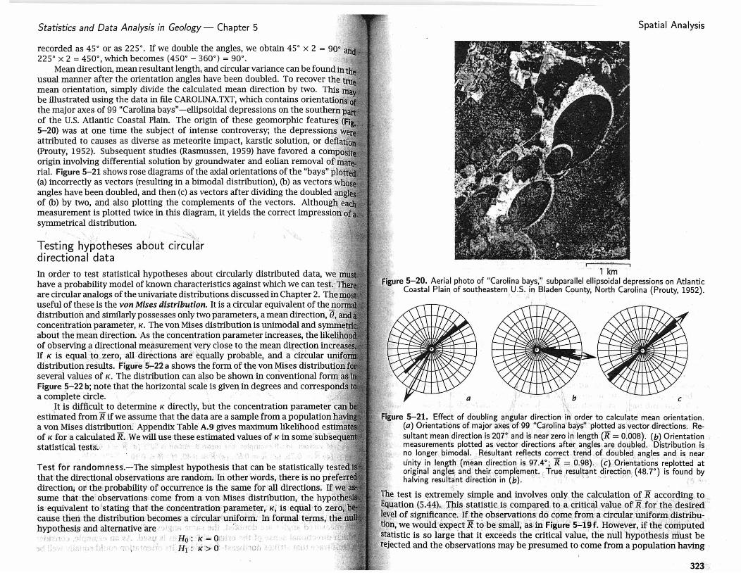
Mean direction, mean resultant length, and circular variance can be found in usual manner after the orientation angles have been doubled. To recover the trlll~-dR mean orientation, simply divide the calculated mean direction by two. This be illustrated using the data in file CAROLINA. TXT, which contains the major axes of 99 "Carolina bays"-ellipsoidal depressions o.n the southern of the U.S. Atlantic Coastal Plain. The origin of these geomorphic features 5-20) was at one time the subject of intense controversy; the depressions attributed to causes as diverse as meteorite impact, karstic solution, or aei1a.~i6n,iilt' (Prouty, 1952). Subsequent studies (Rasmussen, 1959) have favored a cornpc:>Stt1!!ii origin involving differential solution by groundwater and eolian removal rial. Figure 5-21 shows rose diagrams of the axial orientations of the "bays" (a) incorrectly as vectors (resulting in a bimodal distribution), (b) as vectors angles have been doubled, and then (c) as vectors after dividing the doubled of (b) by two, and also plotting the complements of the vectors. Although. measurement is plotted twice in this diagram, it yields the correct impression of symmetrical distribution. ·

• j •• ;-.

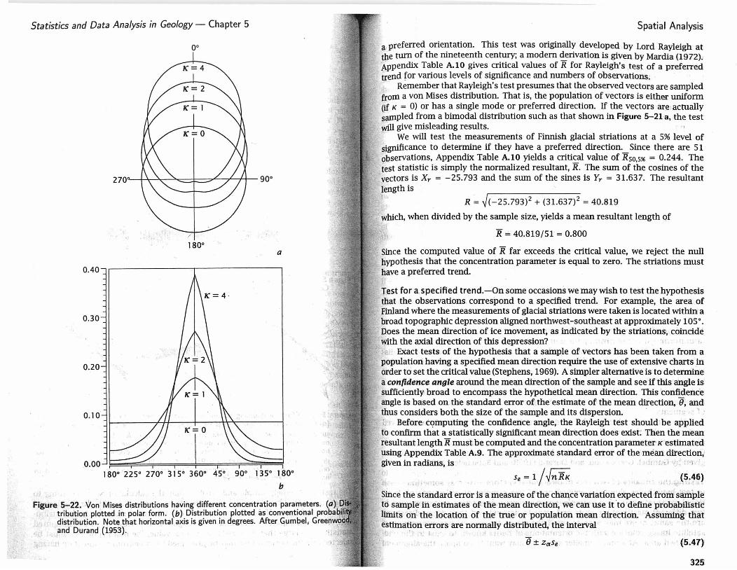
Testing hypotheses about circular directional data In order to test statistical hypotheses about circularly distributed data, we have a probability model of known characteristics against which we can test. are circular analogs of the univariate distributions. discussed in Chapter 2. The useful of these is the von Mises distribution. It is a circular equivalent of the distribution and similarly possesses only two parameters, a mean direction, e, concentration parameter, K. The von Mises distribution is unimodal and about the mean direction. As the concentration parameter increases, the PI<«~I.i.b.oo~ of observing a directional mer-surement~~ry close to th~ mean direqion inr·r""'c""'

If K is equal to zero, all directions are equally probable, and a circular uuJL.lUl·J.U

distribution results. Figure '5-22 a shows the form of the von Mises several values of K. The distribution can also be shown in conventional form Figure 5-22 b; note that the horizontal scale is given 1n degrees and correspon~s a complete circle. . ·

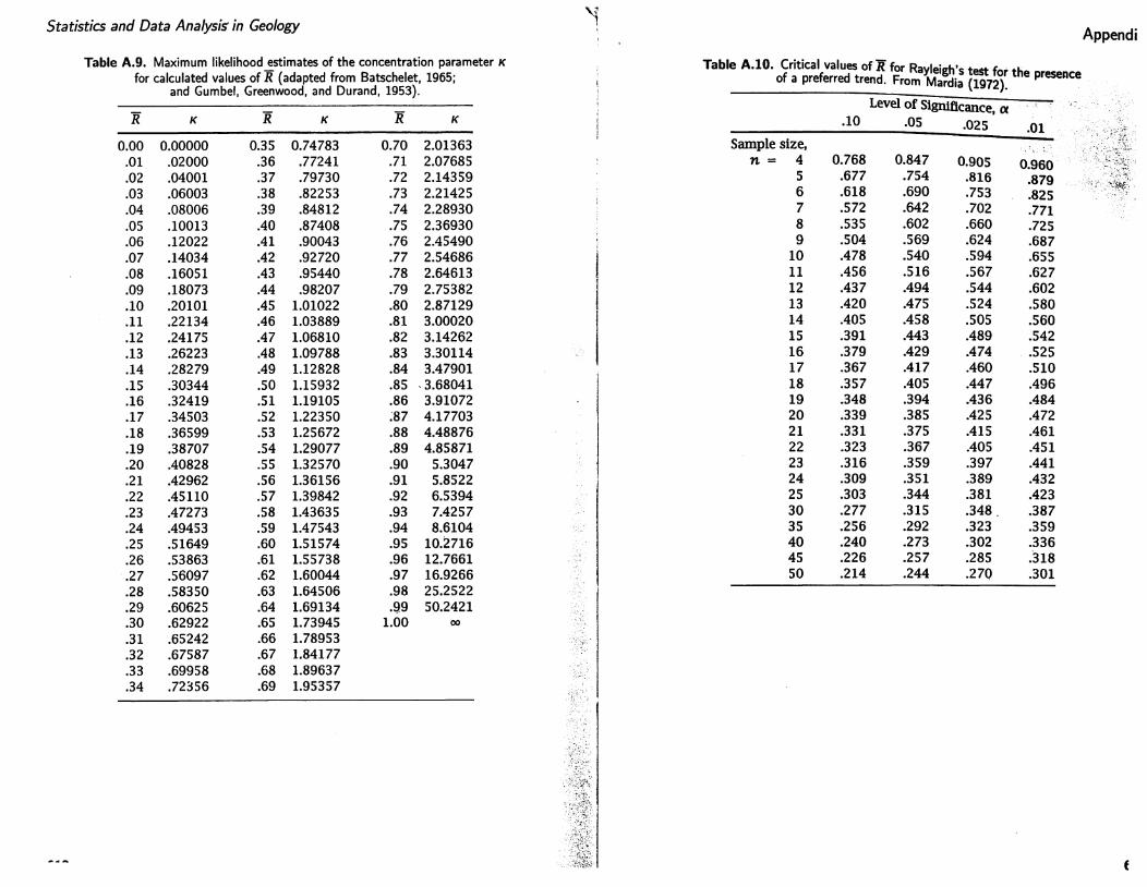
It is difficult to determine K directly, but the concentration parameter can estimated from R if we assume that the data are a sample from a population a von Mises distribution; AppendiX Table A.9 gives maximum likelihood <>ctirn,,t .. a

of K for a calculated R. We will use these estimated values of K in some ,·,. .1u'""Ylucu~ statistical tests.,· , ·

. I· ·\ .. ' ' ;).

Test for randomness.-The simplest hypothesis that can be statistically tested that the directional observations are randoin.·" Iri other words, there is no . direction, or. the probability of occurrence is the same for all directions. If, . sume that the observations come from a von Mises distribution, the h•nnnlth<>-ct

is equivalent to 'statiilg that the concentration parameter, K; is eqtial ·to zero,cl cause then the distribution becomes a circular·unifofm.· In formal: terms, the hypothesis and alternative 'are · ; " , . '-'· ~ · ·. · · . ' · · ''

··1H 1· J , •. r- -: .. •!· ,,, Ho: ·k=Of'l ': !1 c

.-. '"' ) , ., .... I ,, . · , , ~'"; ~ ), Hr: K > 0· -~ ·J.:· !.~·#ut'J

Spatial Analysis

1 km Figure 5-20. Aerial photo of "Carolina bays," subparallel ellipsoidal depressions on Atlantic

Coastal Plain of southeastern U.S. in Bladen County, North Carolina (Prouty, 1952).

c

Figure 5-21. Effect of doubling angular direction i~ order to calculate mean orientation. (a) Orientations of major axes of 99 "Carolina bays" plotted as vector directions. Re-sultant mean direction is 20i• and !s near zero i~ length (R = 0.008). (b) Orientation measurements plotted as vector directions after angles are doubled. Distribution is no longer bimodal. Resultant reflects correct. trend of dciubl~d a·ngles and is near unity in length (mean direction is 97.4°; R = 0.98) :. (c). OrientatiOilS replotted at original angles, and their complemenr True resl!l~ant direction, {48.7•) is found by halving resultant airecticin in (b). . ' ' ' ' ' ' '

The test is ~xtremely simple and involv_es only the ~alculation of R accorcling to Eqqation (5.44).. This statistic. is compared, to a. criticai value of1 R for the . desir~d · level of significance. if the observations do come from· a circular uniform 'distribu­tl!?n. we would exi>e_ct R to b~ $mall, as in Figure' 5-19 f. Ho,wever, if the computed statistic is so large that it exceeds the critical value, the null hypothesis niust be rejected and the observations may be presumed to come from a population having

323 ".

Statistics and Data Analysis in Geology- Chapter 5

oo

/

180° a

0.40

0.30

0.20

0.10

0.00 180° 225° 270° 315° 360° 45° . 90° 135° .180°

b I

Figure 5-22. ·Von Mises distributions having different concentration parameters. . tributiort plotted in. polar form. (b) Distribution plotted as conventional uru1ud1unn

distribution . Note that horizontal axis is given in degrees. After Gumbel 1 and Durand (1953). . , .

Spatial Analysis

a preferred orientation. This test was originally developed by Lord Rayleigh at the turn of the nineteenth century; a modem ~rivation is given by Mardia (1972). Appendix Table A.lO gives critical values of R for Rayleigh's test of a preferred trend for various levels of significance and numbers of observations.

Remember that Rayleigh's test presumes that the observed vectors are sampled from a von Mises distribution. That is, the population of vectors is either uniform (if K = 0) or has a single mode or preferred direction. If the vectors .are· actually sampled from a bimodal distribution such as that shown in Figure 5-21 a, the test will give misleading results.

We will test the measurements of Finnish glacial striations at a 5% level of significance to determine if they have a preferred direction. Since there are 51 observations, Appendix Table A.lO yields a critical value of R50,516 = 0.244. The test statistic is simply the normalized resultant, R. The sum of the cosines of the vectors is Xr = -25.793 and the sum of the sines is Yr = 31.637. The resultant length is

R = ~(-25.793) 2 + (31.637) 2 = 40.819

which, when divided by the sample size, yields a mean resultant length of

R = 40.819/51 = 0.800

Since the computed value of R far exceeds the critical value, we reject the null hypothesis that the concentration parameter is equal to zero. The striations must have a preferred trend.

Test for a specified trend.-On some occasions we may wish to test the hypothesis that the observations correspond to a specified trend. For example, the area of

. Finland where the measurements of glacial striations were taken is located within a broad topographic depression aligned northwest-southeast at approximately 105•. Does the mean direction of ice movement. as indicated by the striations, coincide with the axial direction of this depression? ·

c. Exact tests of the hypothesis that a sample of vectors has been taken: from a population having a specified mean direction require the use of extensive charts in order td set the critical value (Stephens, 1969). A simpler alternative is to detel'IlliD.e a confidence angle around the mean direction of the sample and see if this angle is sufficiently broad to. encompass the hypothetical mean direction. This confidenc'e angle is based on the standard error of the· estimate of the mean direction, e. and· thus considers both the size of the sample and its dispersion. ·' ' · L; Before computing the confidence angle, the Rayleigh test should .be applied to confirm that a statistically significant mean direction does exist. Then the mean resultant length R must be computed and the concentration parameter· K estimated using Appendix Table A.9. The approximate standard error of the mean direction( given in radiansi is 1, r t.i ·~ · ' · ··1

(5.46) _,' . ' ~ . . -

since the standard error is a measure of the chance variation eXpected from sample td sample iri. estimates of. the mean direction, · we can use it to define probabilistic limits ori the location of the true · or population mean direction. Assuinirig that estimat~on errors are normally distributed; the interval · -,

., f ~

0 ± ZaSe . . i (5.47)

325

Statistics and Data Analysis in Geology- Chapter 5

should capture (or include) the true population mean direction oc% of the tin'J.~. example, if we collected 100 random samples of the same size from a ... ~ .... ~· ... u•u"' of vectors and computed the mean directions and 95% confidence intervals each, we would expect that all but about five of those intervals would contciin true mean direction. Of course, we would not know which five of the intervals to capture the true direction, so we must assign a probabilistic caveat to an· of We might,• for example, make the statement that "the interval, plus and many degrees around the mean direction of this particular sample, cm1·t atr.ts' th true population mean direction. The probability that this statement is 1nr·nn,,,...

5%X '·· t. ' 'I ••. ·: ; L{ We have already applied Rayleigh's test and rejected the hypothesis of nn•no,,.,., .. .,

in the observations of the striations. The approximate standard error of the · direction can now be found: · ·. 'r; :;f

s = 1 = --1-· - = 0.0924 radians = 5.29° ·1

e v'51 · 0 .. 8004 : 2.87129 10.826,

Therefore, tbe probability is 95% that Jhe interval ., . . . . .

129:2~ ± 1.9Q >.< 5·.2.9°::

contairls the population mean direction:. In other words, • '· · ' ·' - ';'lj ;·~ ,:jJ I •,! I '. ~

118.8° ::5 e ::5 139.6°

Since thil!· interval doe.s not include the direction of hligiunent of the ·tOJ~O!lfl"al~hli depressionl ~e _must conclude that the. axis of the. depression does ndv cotnotl[f8 With-the mean:direc~on of the striations: \···, A lr, -~ ,. ·~-~, "· ·;. •· · •.

::(·f.·tJ,~:\ .. -.:.-.·~"::J=. r·· !_}n_ j ~~- 1ti! !J,q-:. J

Test of, gpodness .of fit."-A simple nonparametric alternative to the Rayleigh of uiuformity involves dividing the unit circle into a convenient number of . segments~ ; If. these segments are equal in. size and tfie observed· vectors are tributed at random, we should observe approxi.J:hately equal-numbers· of.ve<::tor~JII each segm~nt; . The.number actually observed ·can. be compared to· those' ex])e~:tea by a X~- test. The expected frequency in ea<:h·segment must be at least 5~ should: be· between tt./ 1 S and n 15 . segment!? . The· xl statistic: is ... u,:u~,J•u••t:u, . ...., ....... usuafin,anner (see Eq~ 2.4 5) and has k -1 degrees offteedont, wl!ere k is ·: thle"~lllJI1ibe1 of segments. ·, · ,. 1·· .• :\. ·' ' :.t.>' !. ··::: ::(: c .c :····: · · :' ·.t,.., . ., .,..:bi • ·'l',,The same procedure. can. be u~ed to test the gobctlless of .fit of· the< nh!~PrverJ vector's to other theoretical models, such as a.von Mises distribution with a .,.,,,,.,,.,n concentration> parameter' K great.er; than zerO> anci>a ~pecified; niearr. Cllr•ectJtO:Q. Comp_uting' the expected frequencies; howevei', can be complicated: t J..J\.Ow.J..&IJ•~;., given by Gumber; Greenwood, and Durand (1953) and Batschelet (1965)u;1 '4- ·

.J" , ;; I: ' . ·-;., '~\ \'":' ": '•l~ '}':.,_~- )/.:_:,,..' '~~.·

Testing the equality of two sets of'dihktional vectors.'7'We may An1lt>tinu•<>•t.UUll,

to. ~.E,!,St..~YP,o_tp.~se~ about the eqW.yal~,.c~ , qf. ~o , s~p~~~ or1 c.oll!'!c!ioq~ tiOJ.lal me;~sur!'!inent~. ,Fon exam~le, we,Jlli,I.Y, hayt: . pal~p<!l;We:qt; n;.~ep~sq.rerQ.~d!S ~<;)5 di,ffer~t. stratigraphic units ,and want,,tq; pete.rnWte _if the.lt m.E~~~·1ru~tel"!!.t!ID are the same, or w,e may wish; tq~~ee if fu:e. 9rie.ntation~ o~ . . . satellite image cdiricide with the orientation~ of faults known to exist to graphed area. At a much smaller scale, we may want to comi?are the ali!:JU.l~en

Spatial Analysis

of elongated pores in thin sections from two cored samples of sandstone from a petroleum r~servoir.

The equality of two mean directions may be tested by comparing the vector resultants of the two groups to the vector resultant produced when,the two sets of rneasurements are combined or pooled. If .the two samples actually are drawn from die same population, the resultant of the pooled samples should be approximately equal to the sum of .their two resultants. If the mean directions of the: tWo 1;amples are significantly different, the pooled resultant will be shorter than the suin of their resultants': · <' '

If K is a large value (greater than 10) •. an F-test statistic can be computed by

_ (~-2) (R1 +Rz ~Rp) hn~2 - .· ( n _ R

1 _ Rz) 'J•: '..,. (5.48)

where ri i~> the total number of observations, R1 and Rz are the resultants of the . ~o sampies of vectors, and.Rp is the resultant of the set of vecto~s .after the two grgups haye been pooled. , . . . . . ·. . . . . •. . ·

• .' Using Appendix Table A.9, we can estimate the value of K from :R;,, the length of the mean resultant 0(· the t}VO pooled samples. If K is smallE_!r than 1 b bu,t greater

·} • . , ' . - . , I < • than 2, then a more accurate F-test is ; : 1· 1 ·· · ( ..,

' i ' / .' ' _,- t ,· ' . \ . ., ,

/ _, (: . 3·-) (n- 2) (R1 + R~ , !.... Rp) .hn-z·= ·1 +- . . (5 49)

' ; · i , 8K . .:; ( n - R1 - Rz) 1 •

If K is less\ than 2, s~eciat tables '(such~; thosk mven in Mardia,1972) eri-e necessary. It is also possible t<;> test the equalitY of the concentration paramete:fs of two sets of\rectors; but the. comput'a~ons are invoived. Referito Mardia (197,2)1ror a detailed discussion, and to Gaile and Burt (I 980) for a wor~ed example from geomorphology.

· A fold be)t, expressed topographically as 'the Naga Hills and• therr extensions, oecurs at the jun¢ture between the India!?- subcorltinen~ ~4 the hidochiiiese 'pe.nin-

. sula. Apparently related to .compressive movements that created tile Himalayas, the' fold belt bidudE_!s a s,eri~s(. of subparallel anticlines along the eastern border of Bangiadeslh 'OU,arid gas hci e be~n found in structural traps in t]Jis region; so d~lineati'on of t~e ~old~ -is pf economic a~ weil' as scientific interest. Pr~sumably the~ fo~ds occur, perhaps With: reduced magrutude·, to the west of the Naga1Hills, but are concealed! by mo~em ~ediments deposited by the·GcritgeS'.River and its tributaries . . Unfortunately, reflection seismic data that could reveal the buried structures are

. . .t . . } < -· t • ~ .. ~. ~. •• I' • ·~i ... y ~· \J ' verys:par~e: · · . ...,I. · · ·, ·~ · '' · .. _;: .. ;~·. · < · ·! · ..

Interpretations of Landsat satellit.e image~ of this ·region iridicate numerous lineations1 ofunkno'wn. ori~ It is possible that the ilneation~ rt:fl'e¢t subsurface folds, andj if so, they may provide valuabl clues tb structural geology. and possible petroleum deposits. : . · (.:,. :,:/· ' . : · . i, "·' · ,.'

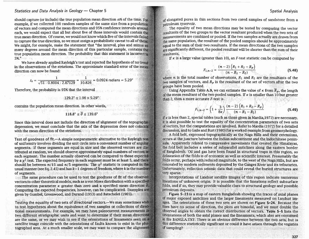
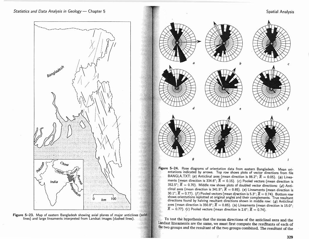
Figu'r~ 5-;23 is a map of easte.rJ1 Bangladesh showing the1traces of_axial planes of major e){posed anticlines· 'and the Hrrger lineaments' measured on Landsat iffi, ag~s. Th,~ qrientations of' these, two sets are shown on· Figure 5.-24.: Because the lines have no 'seiise' of diTection, the plots are bilnodal; and~~ must" double 'the ~bserved angles to 'obtain the cbrred distribution· of vectors. Table' 5-5 list~ the o~ehtati0ris10f b'oth the axiru planes and the lineiUrients, which also afe-contciirted in file BANGIJ\,ixF:. ~hefe· is <hi. obvious difference1~tWe~ the~ two sets1 but is this difference statistically significant or could it have arisen through the vagaries. of sampling? · . ' >, . . · ·.. ., ,'. :'!,,, •

327

Statistics and Data Analysis in Geology- Chapter 5

., ·-- ..... . -....... . _________ ...... ____ ;-·-·- ·-.

Figure 5-23. Map of eastern Bangladesh showi~g axial planes of major a~ticlines (solid lines) and large lineaments interpreted from Landsat images (dashed lmes) . .

Spatial Analysis

a

e

g

Figure 5-24. Rose diagrams of orientation data from eastern Bangladesh. Mean ori­entations indicated by arrows. Top row shows plots of vector directions from file BANGLA .TXT: (a) Anticlinal axes (mean direction is 86.2° ; R = 0:05). (b) Linea­ments (mean direction is 334.6°; R =:· 0.15). (c) Pooled vectors (mean direction is 352.5"; R = 0.70) . Middle row shows plots of doubled vector directions: (d) Anti­clinal axes (mean direction is 341.5"; R = 0.85). (e) Lineaments (mean direction is 30.1°; R = 0.77) . (f) Pooled vectors (mean djr~tion is 5.3°; R = 0.74) . Bottom row shows orientations replotted at original angles and their complements. True resultant directions found by halving resultant directions shown in middle row: (g) Anticlinal axes (mean direction is 350.8°; R = 0.85-). (h) Lineaments (mean direction is 15.0°; R = 0.77) . (i) Pooled vectors (mean direction is 2.6°; R = 0.74) .

To test the hypothesis that the meari directions of the anticlinal axes and the Landsat lineaments are the same, we must first compute the resUltants of each of th_e two groups and the resultant of the two groups combined. The resultant of the

329

Statistics and Data Analysis in Geology- Chapter 5

Table 5-5. Orientation of axial planes of anticlines and Landsat lineations in eastern Bangladesh; measurements

given in degrees clockwise from north .

Anticlinal Axes, n = 34 Landsat Lineaments, n = 36

12 16 14 5 350 32 15 8 192 202 169 163 214 192 16 26 186 186 24 344 356 218 198 221 343 346 161 341 350 18 221 342 339 150 169 336 160 205 35 337 351 156 159 352 2 171 196 14 152 162 341 181 184 246 175 25 348 158 156 354 213 26 212 330 162 20 42 354 13 202

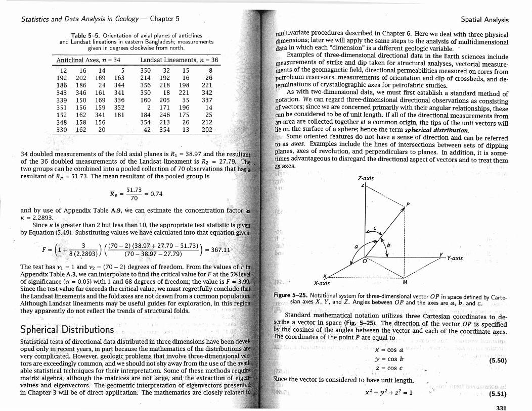
34 doubled measlll'ements of the fold axial planes is R1 = 38.97 and the of the 36 doubled measlU'ements of the Landsat lineament is R2 = 27.79 .. two groups can be combined into a pooled collection of 70 obser-Vations that has resultant of Rp = 51.73. The mean resultant of the pooled group is · \

Rp = 5 ~·~3 = 0.74

and by use of Appendix Table A.9, we can estimate the concentration fa~to~, K = 2.2893. . . .

Since K is greater than 2 but less than 10, the appropriate test staqstic is by Equation (5.49). Substituting values we have calculated into that equatio11

F= (1 .+ 3 ) ((70-2)(38.97.+27..79-51.73)) = 367X1~~-. ' 8(2.2893) (70-38.97-27.79) ' ' .

The test has v1 = 1 and v2 = (70- 2) degrees of freedom. From the values ofF Appendix Table A.3, we can interpolate to find the critical value for F at the 5% of significance (£X= 0.05) with 1 and 68 degrees of freedom; the value is F = Since the test value far exceeds the critical value, we must regretfully conclude the Landsat lineaments and the fold axes are not drawri from a con:llnon Although Landsat lineaments may be useful guides for exploration, :In this they apparently do not reflect the trends of structlll'al folds.

Spherical Distributions . Statistical tests of directional data distributed in three dimensions have been oped ot:lly in recent years, in part because the mathe~atics of the distributions very complicated. However, geologic problems that involve -· · . . . ·-· . ' ~

tors are exceedingly common, and we should not shy away from the use of the able statistical techniques for theit interpretation. Some of these. methods matrix algebra, although· the matrices are no't large; and the' extraction df· values-- and eigenvectors. Tlie geometric' interpretation of eigenvectors' n .. · , >C!Olnn•t

in Chapter 3 will be of direct application. The mathematics ate closely

Spatial Analysis

multivariate procedlll'es described in Chapter 6. Here we deal with three physical djnlensions; later we will apply the same steps to the analysis of multidimensional data in which each "dimension" is a different geologic variable. ·

Examples of three-dimensional directional data in the Earth sciences include measlll'ements of strike and dip taken for structlll'al analyses, vectorial measure­inents of the geomagnetic field, directional permeabilities measured on cores from

· petroleum reservoirs, measlll'ements of orientation and dip of crossbeds, and de-terminations of crystallographic axes for petrofabric studies. ·

As with two-dimensional data, we must first establish a standard method of notation. W,~ can regard three-dimensional directional observations as consisting of vectors; ~mce we are concerned primarily with their angular relationships, these can be cons1dered to be of unit length. If all of the directional measurements from

' an area are collected together at a common origin, the tips of the unit vectors will lie on the Slll'face of a sphere; hence the term spherical distribution.

, Some oriented featlll'es do not have a sense of direction md can be referred to as axes. Examples include the lines of intersections between sets .of dipping planes, axes of revolution, md perpendiculars to plmes. In addition, it is some­times advmtageous to disregard the directional aspect of vectors md to treat them as. axes.

Z-axis

z ------------------- p

y , Y:axis

0 ' '-,,, , _. I //

~- . __ ..... ....... .. ',, ·I ••·

X ----------- ---------------~ -~ ... ~::: ::l<--' '{k. X-axis M

Figure ~-25. Notational system for three-dimensional vector OP in space defined by Caite-!lT. s1an .axe~ X. Y, and Z. Angles between OP and the axes are a, b, and c.. ,

Stmdard mathematic<U notation utilizes three Cartesim ~~orclliJ.ates to de­~S}ibe a ve~tor in space (~ig; .~-;-~5). The direction .of the vect.or OP is specified DY;}he· cosin,e~ of ,the mgles 'Qetween the ve,ctor md each of the coordinate axes. Til~ coordinates df the point P eire equal .to ' ·'

'.I_, t x =cos a

y =cos b I

' z =cos c ·,

Since the vector is considered to have unit len~h, l· ..

x2 + y2 + z2 = 1 . t'J !'I 1._

_,

(5.51)

331

'J Statistics and Data Analysis in Geology 1

Appendi

Table A.9. Maximum likelihood estimates of the concentration parameter K Table A.lO. Critical values of R for Rayleigh's test for the resence for calculated values of R (adapted from Batschelet, 1965; of a preferred trend. From Mardia (1972). P

and Gumbel, Greenwood, and Durand, 1953). Level of Significance, oc

R R K R K K .10 .05 .025 .01 0.00 0.00000 0.35 0.74783 0.70 2.01363 Sample size, ,·,.'

.01 .02000 .36 .77241 .71 2.07685 n= 4 0.768 0.847 0.905 0.960

.02 .04001 .37 .79730 .72 2.14359 5 .677 .754 .816 .879

.03 .06003 .38 .82253 .73 2.21425 6 .618 .690 .753 .825

.04 .08006 .39 .84812 .74 2.28930 7 .572 .642 .702 .771

.OS .10013 .40 .87408 .75 2.36930 8 .535 .602 .660 .725

.06 .12022 .41 .90043 .76 2.45490 9 .504 .569 .624 .687

.07 .14034 .42 .92720 .77 2.54686 10 .478 .540 .594 .655

.08 .16051 .43 .95440 .78 2.64613 11 .456 .516 .567 .627

.09 .18073 .44 .98207 .79 2.75382 12 .437 .494 .544 .602

.10 .20101 .45 1.01022 .80 2.87129 13 .420 .475 .524 .580

.11 .22134 .46 1.03889 .81 3.00020 14 .405 .458 .505 .560

.12 .24175 .47 1.06810 .82 3.14262 15 .391 .443 .489 .542

.13 .26223 .48 1.09788 .83 3.30114 16 .379 .429 .474 .525

.14 .28279 .49 1.12828 .84 3.47901 17 .367 .417 .460 .510

.15 .30344 .so 1.15932 .85 '3.68041 18 .357 .405 .447 .496

.16 .32419 .51 1.19105 .86 3.91072 19 .348 .394 .436 .484

.17 .34503 .52 1.22350 ;s? 4.17703 20 .339 .385 .425 .472

.18 .36599 .53 1.25672 .88 4.48876 21 .331 .375 .415 .461

.19 .38707 .54 1.29077 .89 4.85871 22 .323 .367 .405 .451

.20 .40828 .55 1.32570 .90 5.3047 23 .316 .359 .397 .441

.21 .42962 .56 1.36156 .91 5.8522 24 .309 .351 .389 .432

.22 .45110 .57 1.39842 .92 6.5394 25 .303 .344 .381 .423

.23 .47273 .58 1.43635 .93 7.4257 30 .277 . 315 .348 . .387

.24 .49453 .59 1.47543 .94 8.6104 35 .256 .292 .323 .359

.25 .51649 .60 1.51574 .95 10.2716 40 .240 .273 .302 .336

.26 .53863 .61 1.55738 .96 12.7661 45 .226 .257 .285 .318

.27 .56097 .62 1.60044 .97 16.9266 so .214 .244 .270 .301

.28 .58350 .63 1.64506 .98 25.2522

.29 .60625 .64 1.69134 .Q9 50.2421

.30 .62922 .65 1.73945 1.00 00

.31 .65242 .66 1.78953

.32 .67587 .67 1.84177

.33 .69958 .68 1.89637

.34 .72356 .69 1.95357