Statistics 5100 Summer 2012 Exam 2 - Utah State … 5100 Summer 2012 Exam 2. ... Root MSE . 1777.40294 . R-Square . 0.3949 . Dependent Mean . ... eastMS 1 1.0002 0.4205 5.6567 0.0174

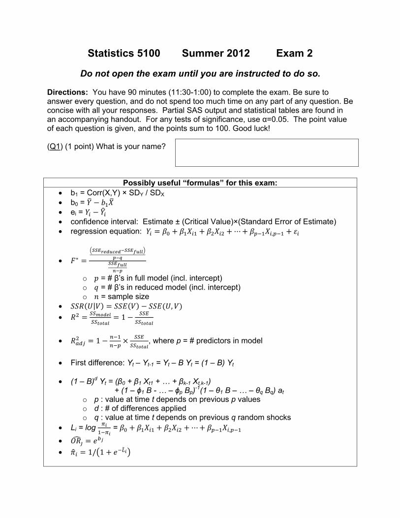
Statistics 5100 Summer 2012 Exam 2

Do not open the exam until you are instructed to do so. Directions: You have 90 minutes (11:30-1:00) to complete the exam. Be sure to answer every question, and do not spend too much time on any part of any question. Be concise with all your responses. Partial SAS output and statistical tables are found in an accompanying handout. For any tests of significance, use α=0.05. The point value of each question is given, and the points sum to 100. Good luck! (Q1) (1 point) What is your name?

Possibly useful “formulas” for this exam: • b1 = Corr(X,Y) × SDY / SDX • b0 = 𝑌� − 𝑏1𝑋� • ei = 𝑌𝑖 − 𝑌�𝑖 • confidence interval: Estimate ± (Critical Value)×(Standard Error of Estimate) • regression equation: 𝑌𝑖 = 𝛽0 + 𝛽1𝑋𝑖1 + 𝛽2𝑋𝑖2 + ⋯+ 𝛽𝑝−1𝑋𝑖,𝑝−1 + 𝜀𝑖

• 𝐹∗ =�𝑆𝑆𝐸𝑟𝑒𝑑𝑢𝑐𝑒𝑑−𝑆𝑆𝐸𝑓𝑢𝑙𝑙�

𝑝−𝑞𝑆𝑆𝐸𝑓𝑢𝑙𝑙𝑛−𝑝

o 𝑝 = # β’s in full model (incl. intercept) o 𝑞 = # β’s in reduced model (incl. intercept) o 𝑛 = sample size

• 𝑆𝑆𝑅(𝑈|𝑉) = 𝑆𝑆𝐸(𝑉) − 𝑆𝑆𝐸(𝑈,𝑉) • 𝑅2 = 𝑆𝑆𝑚𝑜𝑑𝑒𝑙

𝑆𝑆𝑡𝑜𝑡𝑎𝑙= 1 − 𝑆𝑆𝐸

𝑆𝑆𝑡𝑜𝑡𝑎𝑙

• 𝑅𝑎𝑑𝑗2 = 1 − 𝑛−1

𝑛−𝑝× 𝑆𝑆𝐸

𝑆𝑆𝑡𝑜𝑡𝑎𝑙, where p = # predictors in model

• First difference: Yt – Yt-1 = Yt – B Yt = (1 – B) Yt

• (1 – B)d Yt = (β0 + β1 Xt1 + … + βk-1 Xt,k-1)

+ (1 – ϕ1 B - … – ϕp Bp)-1(1 – θ1 B – … – θq Bq) at o p : value at time t depends on previous p values o d : # of differences applied o q : value at time t depends on previous q random shocks

• Li = log 𝜋𝑖1−𝜋𝑖

= 𝛽0 + 𝛽1𝑋𝑖1 + 𝛽2𝑋𝑖2 + ⋯+ 𝛽𝑝−1𝑋𝑖,𝑝−1

• 𝑂𝑅𝚥� = 𝑒𝑏𝑗 • 𝜋�𝑖 = 1/�1 + 𝑒−𝐿�𝑖�

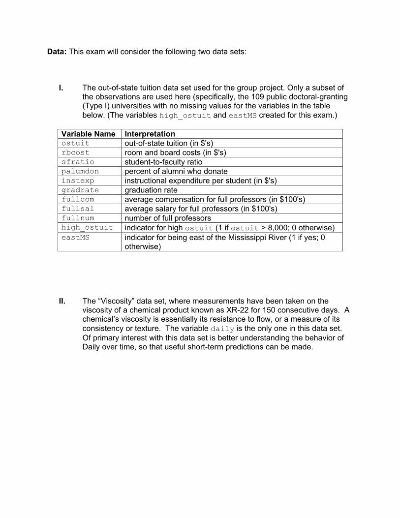
Data: This exam will consider the following two data sets:

I. The out-of-state tuition data set used for the group project. Only a subset of the observations are used here (specifically, the 109 public doctoral-granting (Type I) universities with no missing values for the variables in the table below. (The variables high_ostuit and eastMS created for this exam.)

Variable Name Interpretation ostuit out-of-state tuition (in $'s) rbcost room and board costs (in $'s) sfratio student-to-faculty ratio palumdon percent of alumni who donate instexp instructional expenditure per student (in $'s) gradrate graduation rate fullcom average compensation for full professors (in $100's) fullsal average salary for full professors (in $100's) fullnum number of full professors high_ostuit indicator for high ostuit (1 if ostuit > 8,000; 0 otherwise) eastMS indicator for being east of the Mississippi River (1 if yes; 0

otherwise)

II. The “Viscosity” data set, where measurements have been taken on the viscosity of a chemical product known as XR-22 for 150 consecutive days. A chemical’s viscosity is essentially its resistance to flow, or a measure of its consistency or texture. The variable daily is the only one in this data set. Of primary interest with this data set is better understanding the behavior of Daily over time, so that useful short-term predictions can be made.

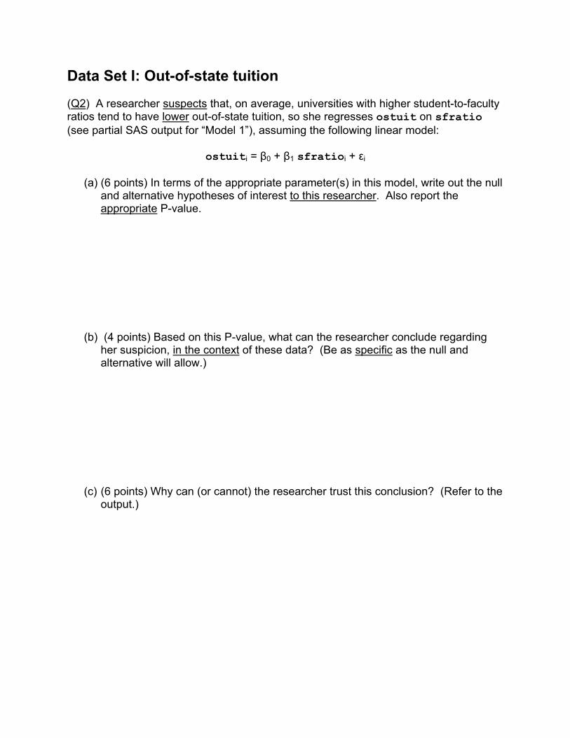
Data Set I: Out-of-state tuition (Q2) A researcher suspects that, on average, universities with higher student-to-faculty ratios tend to have lower out-of-state tuition, so she regresses ostuit on sfratio (see partial SAS output for “Model 1”), assuming the following linear model:

ostuiti = β0 + β1 sfratioi + εi

(a) (6 points) In terms of the appropriate parameter(s) in this model, write out the null and alternative hypotheses of interest to this researcher. Also report the appropriate P-value.

(b) (4 points) Based on this P-value, what can the researcher conclude regarding her suspicion, in the context of these data? (Be as specific as the null and alternative will allow.)

(c) (6 points) Why can (or cannot) the researcher trust this conclusion? (Refer to the output.)

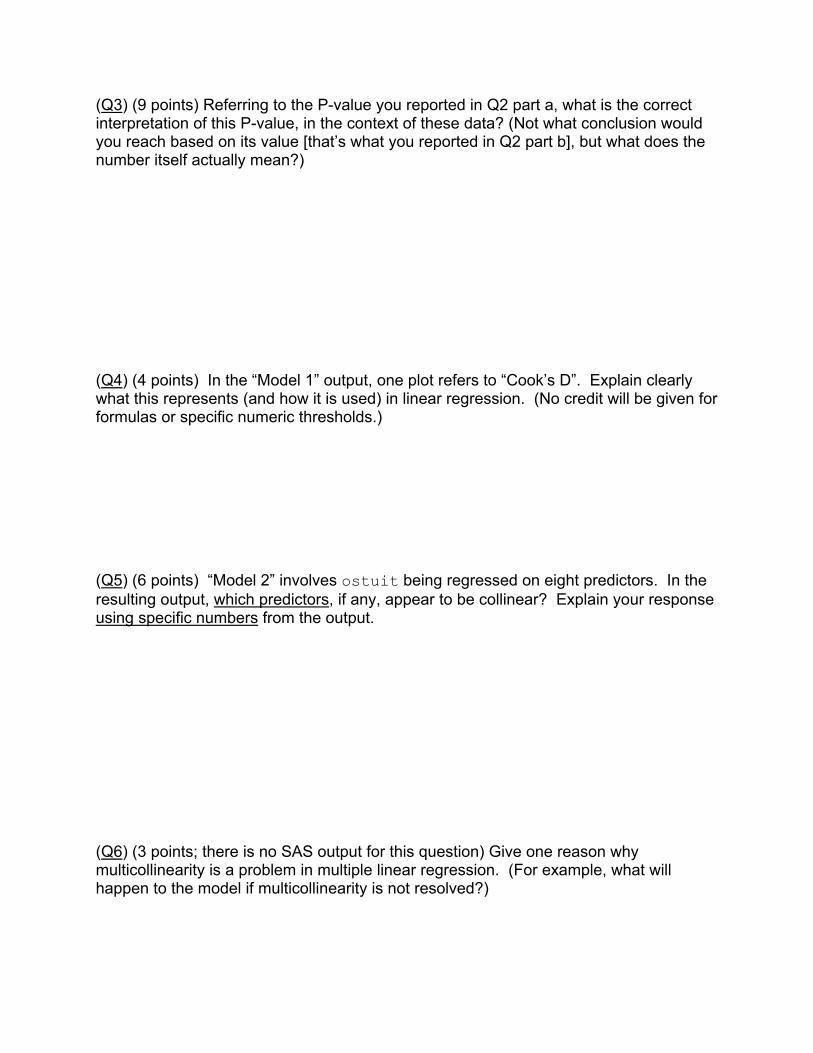
(Q3) (9 points) Referring to the P-value you reported in Q2 part a, what is the correct interpretation of this P-value, in the context of these data? (Not what conclusion would you reach based on its value [that’s what you reported in Q2 part b], but what does the number itself actually mean?) (Q4) (4 points) In the “Model 1” output, one plot refers to “Cook’s D”. Explain clearly what this represents (and how it is used) in linear regression. (No credit will be given for formulas or specific numeric thresholds.)

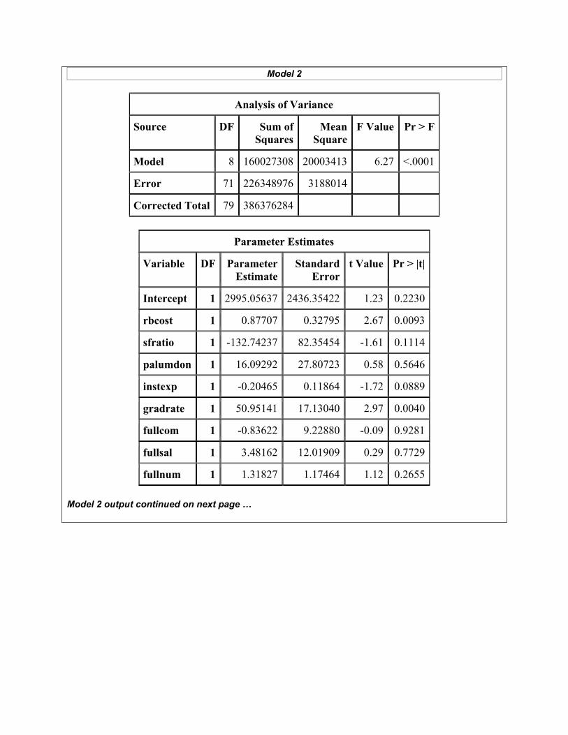
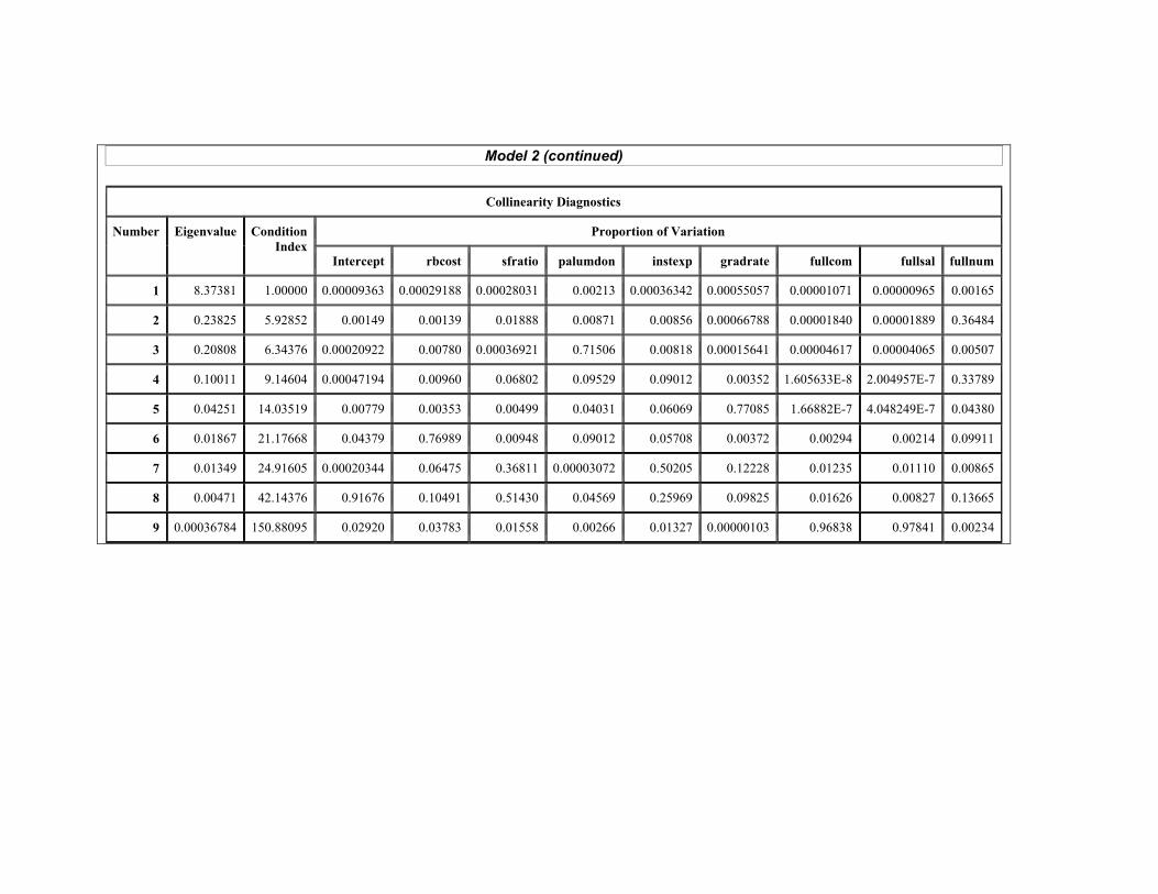
(Q5) (6 points) “Model 2” involves ostuit being regressed on eight predictors. In the resulting output, which predictors, if any, appear to be collinear? Explain your response using specific numbers from the output.

(Q6) (3 points; there is no SAS output for this question) Give one reason why multicollinearity is a problem in multiple linear regression. (For example, what will happen to the model if multicollinearity is not resolved?)

(Q7) (5 points) If you know there is collinearity involving two predictors, what does that tell you about their interaction in a linear regression model? (No output is provided for this question.)

(Q8) (5 points) What proportion of the variation in out-of-state tuition is explained by its linear relationship with the eight predictors in “Model 2”?

(Q9) (5 points) “Model 3” involves ostuit being regressed on five predictors. Models 1-3 were fit using 80 randomly selected universities (of the 109 possible). The Model 3 fit was used to calculate predicted ostuit values for the remaining 29 universities, and their mean squared prediction error (MSPR) was calculated to be about 3.6 million (not shown in output). What can be concluded from this MSPR value? (Provide numerical justification.) (Q10) (6 points) One of the parameter estimates in the “Model 3” output is reported as 62.09706. What is the correct interpretation of this number?

(Q11) (8 points) “Model 4” is the logistic regression model used to predict the probability of high out-of-state tuition (high_ostuit=1) based on which side of the Mississippi River the university falls (eastMS).

(a) (6 points) What is the correct interpretation of the estimated eastMS effect?

(b) (2 points) What can be concluded from the plot following the “Model 4” output?

(c) (6 points) Based on the “Model 4” fit, what is the predicted probability that Utah State University would have high out-of-state tuition?

~~~~~~~~~~~~~~~~~~~~~~~~~~~~~~~~~~~~~~~~~~~~~~~~~~ Data Set II: Viscosity (Q12) (6 points) The “Viscosity ARIMA Output” reports the PROC ARIMA output for these data, with no predictor variables used. Referring to this output, what evidence is there of stationarity?

(Q13) (3 points) Referring again to the “Viscosity ARIMA Output”, what numerical evidence is there of significant dependence structure? (Q14) (8 points) Someone has proposed AR(2), MA(2), and ARIMA(2,0,1) models as possibly appropriate for these data. Based on the “Viscosity ARIMA Output” SAC and SPAC plots, which of these models appears most appropriate, and why? (Q15) (8 points) Each of the three proposed models are fit to the data (with partial output reported in the handout). For the model you selected in Q14, what can you say about its adequacy? (Refer to both numerical and graphical output.) (Q16) (1 point) What topic(s) did you study most that did not appear on this exam?

Output and Tables for Summer 2012 STAT 5100 Exam 2

Model 1

Analysis of Variance

Source DF Sum of Squares

Mean Square

F Value Pr > F

Model 1 16321286 16321286 3.44 0.0674

Error 78 370054998 4744295

Corrected Total 79 386376284

Parameter Estimates

Variable DF Parameter Estimate

Standard Error

t Value Pr > |t|

Intercept 1 9601.52327 1099.56418 8.73 <.0001

sfratio 1 -123.41286 66.53790 -1.85 0.0674

Model 2



Mean Square

F Value Pr > F

Model 8 160027308 20003413 6.27 <.0001

Error 71 226348976 3188014


Parameter Estimates


Standard Error

t Value Pr > |t|

Intercept 1 2995.05637 2436.35422 1.23 0.2230

rbcost 1 0.87707 0.32795 2.67 0.0093

sfratio 1 -132.74237 82.35454 -1.61 0.1114

palumdon 1 16.09292 27.80723 0.58 0.5646

instexp 1 -0.20465 0.11864 -1.72 0.0889

gradrate 1 50.95141 17.13040 2.97 0.0040

fullcom 1 -0.83622 9.22880 -0.09 0.9281

fullsal 1 3.48162 12.01909 0.29 0.7729

fullnum 1 1.31827 1.17464 1.12 0.2655 Model 2 output continued on next page …

Model 2 (continued)

Collinearity Diagnostics

Number Eigenvalue Condition Index

Proportion of Variation

Intercept rbcost sfratio palumdon instexp gradrate fullcom fullsal fullnum

1 8.37381 1.00000 0.00009363 0.00029188 0.00028031 0.00213 0.00036342 0.00055057 0.00001071 0.00000965 0.00165

2 0.23825 5.92852 0.00149 0.00139 0.01888 0.00871 0.00856 0.00066788 0.00001840 0.00001889 0.36484

3 0.20808 6.34376 0.00020922 0.00780 0.00036921 0.71506 0.00818 0.00015641 0.00004617 0.00004065 0.00507

4 0.10011 9.14604 0.00047194 0.00960 0.06802 0.09529 0.09012 0.00352 1.605633E-8 2.004957E-7 0.33789

5 0.04251 14.03519 0.00779 0.00353 0.00499 0.04031 0.06069 0.77085 1.66882E-7 4.048249E-7 0.04380

6 0.01867 21.17668 0.04379 0.76989 0.00948 0.09012 0.05708 0.00372 0.00294 0.00214 0.09911

7 0.01349 24.91605 0.00020344 0.06475 0.36811 0.00003072 0.50205 0.12228 0.01235 0.01110 0.00865

8 0.00471 42.14376 0.91676 0.10491 0.51430 0.04569 0.25969 0.09825 0.01626 0.00827 0.13665

9 0.00036784 150.88095 0.02920 0.03783 0.01558 0.00266 0.01327 0.00000103 0.96838 0.97841 0.00234

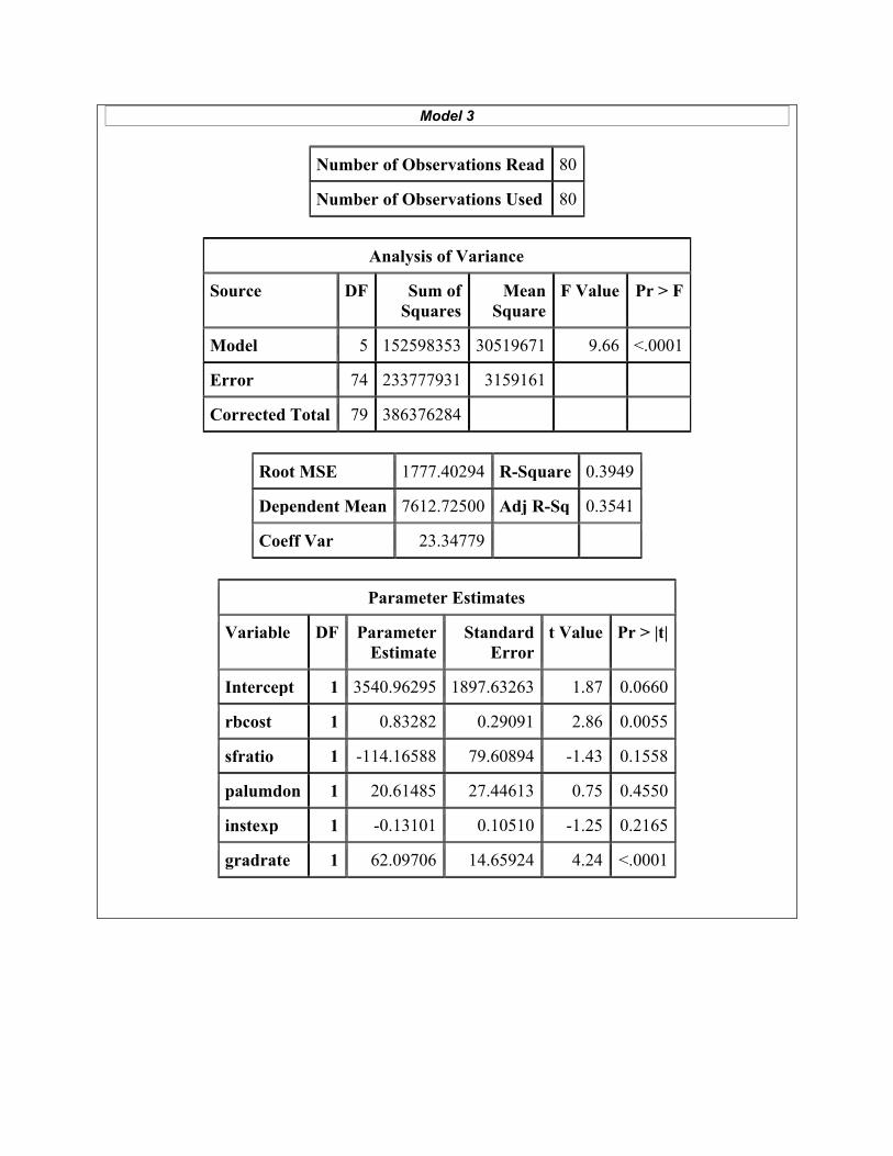
Model 3

Number of Observations Read 80

Number of Observations Used 80



Mean Square

F Value Pr > F

Model 5 152598353 30519671 9.66 <.0001

Error 74 233777931 3159161


Root MSE 1777.40294 R-Square 0.3949

Dependent Mean 7612.72500 Adj R-Sq 0.3541

Coeff Var 23.34779

Parameter Estimates


Standard Error

t Value Pr > |t|

Intercept 1 3540.96295 1897.63263 1.87 0.0660

rbcost 1 0.83282 0.29091 2.86 0.0055

sfratio 1 -114.16588 79.60894 -1.43 0.1558

palumdon 1 20.61485 27.44613 0.75 0.4550

instexp 1 -0.13101 0.10510 -1.25 0.2165

gradrate 1 62.09706 14.65924 4.24 <.0001

Model 4

Response Profile

Ordered Value

high_ostuit Total Frequency

1 0 68

2 1 41

Probability modeled is high_ostuit=1. Convergence criterion (GCONV=1E-8) satisfied.

Analysis of Maximum Likelihood Estimates

Parameter DF Estimate Standard Error

Wald Chi-Square

Pr > ChiSq

Intercept 1 -1.0986 0.3333 10.8625 0.0010

eastMS 1 1.0002 0.4205 5.6567 0.0174

Odds Ratio Estimates

Effect Point Estimate 95% Wald Confidence Limits

eastMS 2.719 1.192 6.199

Viscosity ARIMA Output

The ARIMA Procedure

Name of Variable = daily

Mean of Working Series 35.20133

Standard Deviation 2.922008

Number of Observations 150

Autocorrelation Check for White Noise

To Lag Chi-Square DF Pr > ChiSq Autocorrelations

6 46.31 6 <.0001 -0.415 0.319 0.049 0.004 -0.114 0.109

12 50.46 12 <.0001 -0.110 0.000 0.037 -0.042 -0.083 0.059

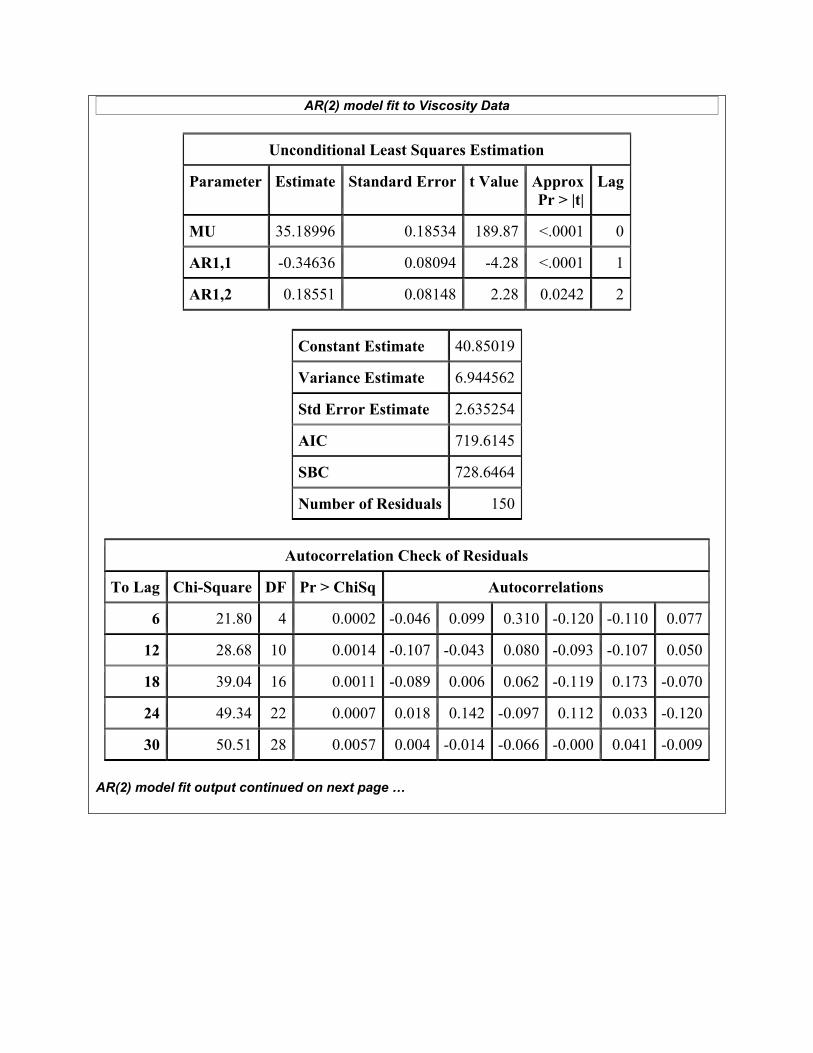
AR(2) model fit to Viscosity Data

Unconditional Least Squares Estimation

Parameter Estimate Standard Error t Value Approx Pr > |t|

Lag

MU 35.18996 0.18534 189.87 <.0001 0

AR1,1 -0.34636 0.08094 -4.28 <.0001 1

AR1,2 0.18551 0.08148 2.28 0.0242 2

Constant Estimate 40.85019

Variance Estimate 6.944562

Std Error Estimate 2.635254

AIC 719.6145

SBC 728.6464

Number of Residuals 150

Autocorrelation Check of Residuals

To Lag Chi-Square DF Pr > ChiSq Autocorrelations

6 21.80 4 0.0002 -0.046 0.099 0.310 -0.120 -0.110 0.077

12 28.68 10 0.0014 -0.107 -0.043 0.080 -0.093 -0.107 0.050

18 39.04 16 0.0011 -0.089 0.006 0.062 -0.119 0.173 -0.070

24 49.34 22 0.0007 0.018 0.142 -0.097 0.112 0.033 -0.120

30 50.51 28 0.0057 0.004 -0.014 -0.066 -0.000 0.041 -0.009 AR(2) model fit output continued on next page …

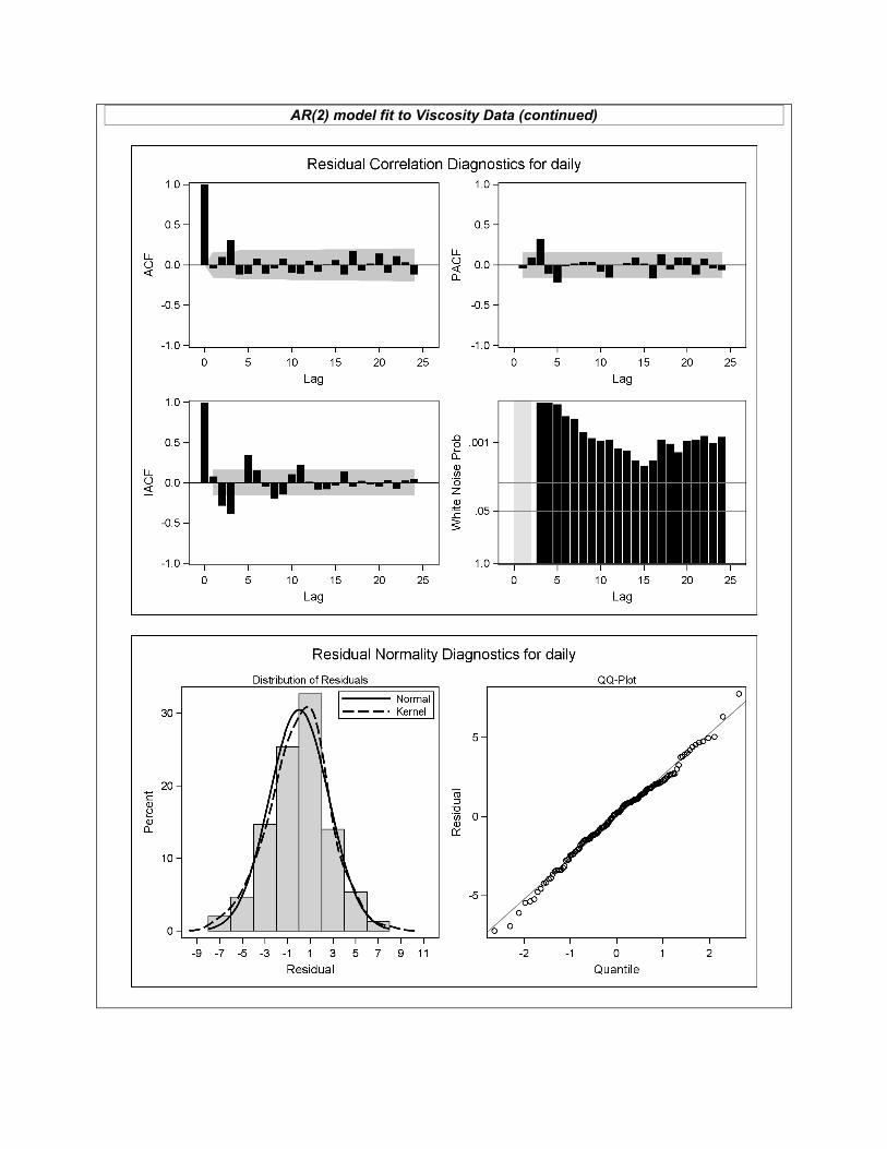
AR(2) model fit to Viscosity Data (continued)

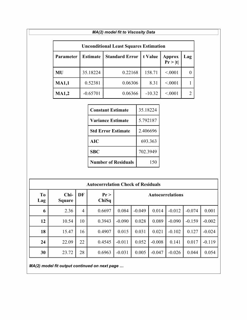
MA(2) model fit to Viscosity Data



Lag

MU 35.18224 0.22168 158.71 <.0001 0

MA1,1 0.52381 0.06306 8.31 <.0001 1

MA1,2 -0.65701 0.06366 -10.32 <.0001 2




AIC 693.363

SBC 702.3949



To Lag

Chi-Square

DF Pr > ChiSq

Autocorrelations

6 2.36 4 0.6697 0.084 -0.049 0.014 -0.012 -0.074 0.001

12 10.54 10 0.3943 -0.090 0.028 0.089 -0.090 -0.159 -0.002

18 15.47 16 0.4907 0.015 0.031 0.021 -0.102 0.127 -0.024

24 22.09 22 0.4545 -0.011 0.052 -0.008 0.141 0.017 -0.119

30 23.72 28 0.6963 -0.031 0.005 -0.047 -0.026 0.044 0.054

MA(2) model fit output continued on next page …

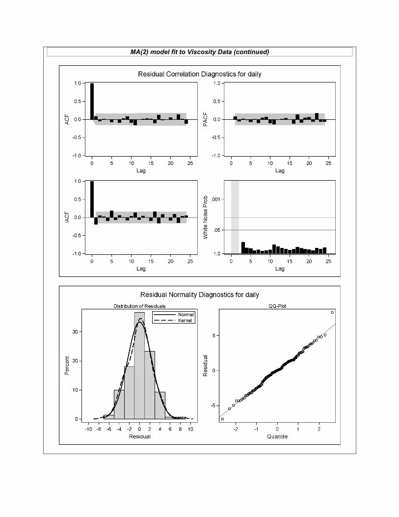
MA(2) model fit to Viscosity Data (continued)

ARIMA(2,0,1) model fit to Viscosity Data



Lag

MU 35.18556 0.24078 146.13 <.0001 0

MA1,1 0.46378 0.24570 1.89 0.0611 1

AR1,1 0.10739 0.22678 0.47 0.6365 1

AR1,2 0.42498 0.09920 4.28 <.0001 2




AIC 715.6398

SBC 727.6824



To Lag

Chi-Square

DF Pr > ChiSq

Autocorrelations

6 18.59 3 0.0003 -0.047 0.050 0.244 -0.159 -0.166 0.047

12 25.62 9 0.0024 -0.111 -0.034 0.087 -0.089 -0.111 0.045

18 34.85 15 0.0026 -0.077 0.010 0.060 -0.113 0.164 -0.070

24 44.82 21 0.0018 0.016 0.136 -0.085 0.116 0.033 -0.125

30 46.20 27 0.0121 -0.006 -0.014 -0.065 0.005 0.054 0.005

ARIMA(2,0,1) model fit continued on next page …

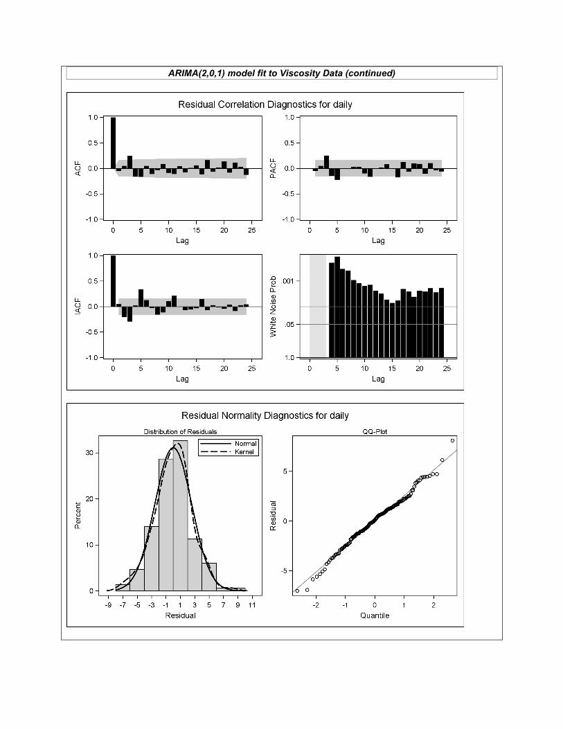
ARIMA(2,0,1) model fit to Viscosity Data (continued)

Documents

Statistics 5100 Summer 2012 Exam 2 - Utah State … 5100 Summer 2012 Exam 2. ... Root MSE . 1777.40294 . R-Square . 0.3949 . Dependent Mean . ... eastMS 1 1.0002 0.4205 5.6567 0.0174