Embed Size (px)
Citation preview
STATISTICS 450/850
Estimation and HypothesisTesting
Supplementary Lecture Notes
Don L. McLeish and Cyntha A. StruthersDept. of Statistics and Actuarial Science
University of Waterloo Waterloo, Ontario, Canada
Winter 2013
Contents
1 Properties of Estimators 1
1.1 Prerequisite Material . . . . . . . . . . . . . . . . . . . . 1
1.2 Introduction . . . . . . . . . . . . . . . . . . . . . . . . . 1
1.3 Unbiasedness and Mean Square Error . . . . . . . . . 4
1.4 Sufficiency . . . . . . . . . . . . . . . . . . . . . . . . . . . 10
1.5 Minimal Sufficiency . . . . . . . . . . . . . . . . . . . . . 16
1.6 Completeness . . . . . . . . . . . . . . . . . . . . . . . . . 18
1.7 The Exponential Family . . . . . . . . . . . . . . . . . . 23
1.8 Ancillarity . . . . . . . . . . . . . . . . . . . . . . . . . . . 33
2 Maximum Likelihood Estimation 39
2.1 Maximum Likelihood Method- One Parameter . . . . . . . . . . . . . . . . . . . . . . 39
2.2 Principles of Inference . . . . . . . . . . . . . . . . . . . 50
2.3 Properties of the Score and Information- Regular Model . . . . . . . . . . . . . . . . . . . . . . . 52
2.4 Maximum Likelihood Method- Multiparameter . . . . . . . . . . . . . . . . . . . . . . 54
2.5 Incomplete Data and The E.M. Algorithm . . . . . . 67
2.6 The Information Inequality . . . . . . . . . . . . . . . . 75
2.7 Asymptotic Properties of M.L.Estimators - One Parameter . . . . . . . . . . . . . . . 79
2.8 Interval Estimators . . . . . . . . . . . . . . . . . . . . . 82
2.9 Asymptotic Properties of M.L.Estimators - Multiparameter . . . . . . . . . . . . . . 92
2.10 Nuisance Parameters andM.L. Estimation . . . . . . . . . . . . . . . . . . . . . . . 108
2.11 Problems with M.L. Estimators . . . . . . . . . . . . . 109
2.12 Historical Notes . . . . . . . . . . . . . . . . . . . . . . . 111
1
0 CONTENTS
3 Other Methods of Estimation 1133.1 Best Linear Unbiased Estimators . . . . . . . . . . . . 1133.2 Equivariant Estimators . . . . . . . . . . . . . . . . . . . 1153.3 Estimating Equations . . . . . . . . . . . . . . . . . . . . 1193.4 Bayes Estimation . . . . . . . . . . . . . . . . . . . . . . 124
4 Hypothesis Tests 1354.1 Introduction . . . . . . . . . . . . . . . . . . . . . . . . . 1354.2 Uniformly Most Powerful Tests . . . . . . . . . . . . . 1384.3 Locally Most Powerful Tests . . . . . . . . . . . . . . . 1444.4 Likelihood Ratio Tests . . . . . . . . . . . . . . . . . . . 1464.5 Score and Maximum Likelihood Tests . . . . . . . . . 1534.6 Bayesian Hypothesis Tests . . . . . . . . . . . . . . . . 155
5 Appendix 1575.1 Inequalities and Useful Results . . . . . . . . . . . . . 1575.2 Distributional Results . . . . . . . . . . . . . . . . . . . 1595.3 Limiting Distributions . . . . . . . . . . . . . . . . . . . 1685.4 Proofs . . . . . . . . . . . . . . . . . . . . . . . . . . . . . 171
Chapter 1
Properties of Estimators
1.1 Prerequisite Material
The following topics should be reviewed:
1. Tables of special discrete and continuous distributions including themultivariate normal distribution. Location and scale parameters.
2. Distribution of a transformation of one or more random variablesincluding change of variable(s).
3. Moment generating function of one or more random variables.
4. Multiple linear regression.
5. Limiting distributions: convergence in probability and convergence indistribution.
1.2 Introduction
Before beginning a discussion of estimation procedures, we assume thatwe have designed and conducted a suitable experiment and collected dataX1, . . . ,Xn, where n, the sample size, is fixed and known. These dataare expected to be relevant to estimating a quantity of interest θ whichwe assume is a statistical parameter, for example, the mean of a normaldistribution. We assume we have adopted a model which specifies the linkbetween the parameter θ and the data we obtained. The model is theframework within which we discuss the properties of our estimators. Ourmodel might specify that the observations X1, . . . ,Xn are independent with
1
2 CHAPTER 1. PROPERTIES OF ESTIMATORS
a normal distribution, mean θ and known variance σ2 = 1. Usually, as here,the only unknown is the parameter θ. We have specified completely the jointdistribution of the observations up to this unknown parameter.
1.2.1 Note:
We will sometimes denote our data more compactly by the random vectorX = (X1, . . . ,Xn).
The model, therefore, can be written in the form f (x; θ) ; θ ∈ Ω whereΩ is the parameter space or set of permissible values of the parameter andf (x; θ) is the probability (density) function.
1.2.2 Definition
A statistic, T (X), is a function of the data X which does not depend onthe unknown parameter θ.
Note that although a statistic, T (X), is not a function of θ, its distrib-ution can depend on θ.An estimator is a statistic considered for the purpose of estimating a
given parameter. It is our aim to find a “good” estimator of the parameterθ.In the search for good estimators of θ it is often useful to know if θ is a
location or scale parameter.
1.2.3 Location and Scale Parameters
Suppose X is a continuous random variable with p.d.f. f(x; θ).Let F0 (x) = F (x; θ = 0) and f0 (x) = f (x; θ = 0). The parameter θ is
called a location parameter of the distribution if
F (x; θ) = F0 (x− θ) , θ ∈ <
or equivalently
f(x; θ) = f0(x− θ), θ ∈ <.
Let F1 (x) = F (x; θ = 1) and f1 (x) = f (x; θ = 1). The parameter θ iscalled a scale parameter of the distribution if
F (x; θ) = F1
³xθ
´, θ > 0
1.2. INTRODUCTION 3
or equivalently
f(x; θ) =1
θf1(x
θ), θ > 0.
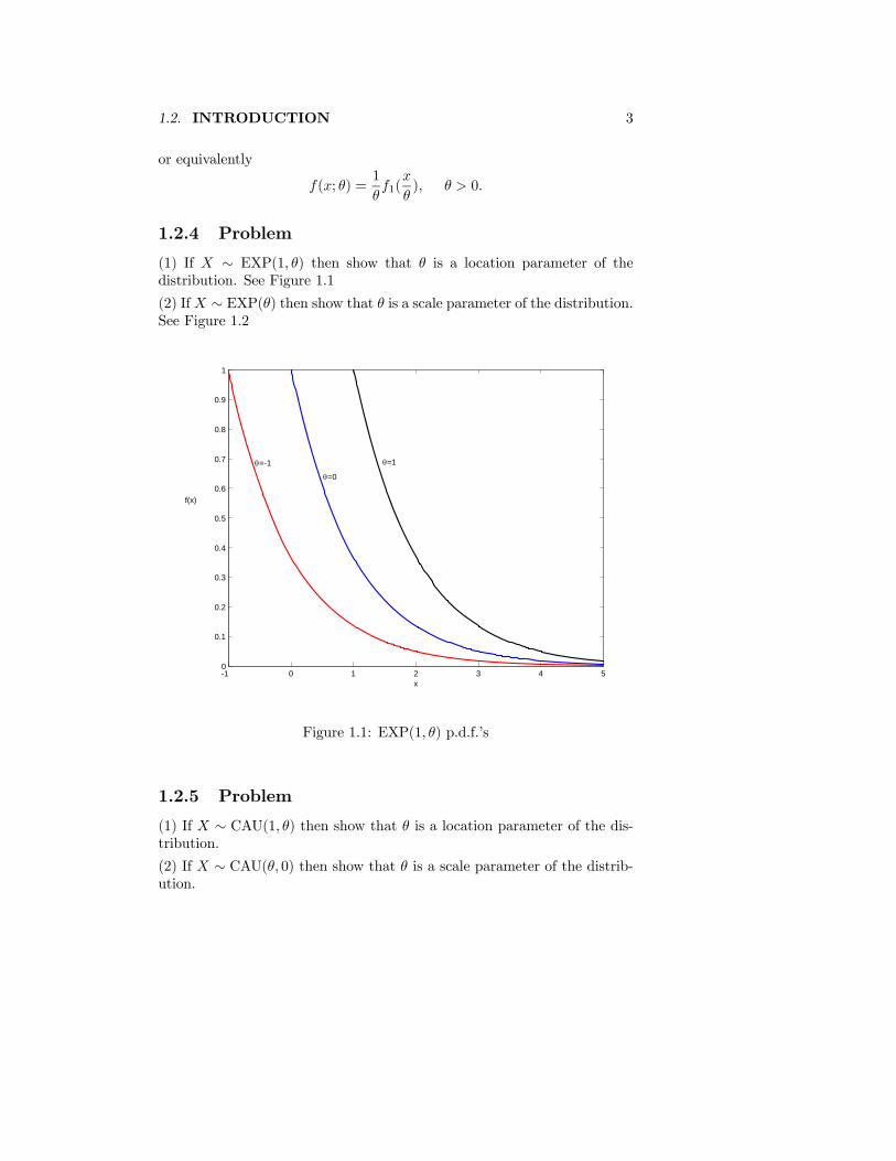
1.2.4 Problem
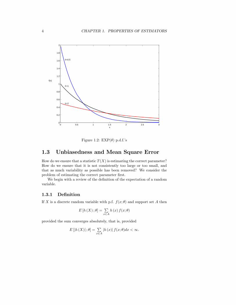
(1) If X ∼ EXP(1, θ) then show that θ is a location parameter of thedistribution. See Figure 1.1
(2) IfX ∼ EXP(θ) then show that θ is a scale parameter of the distribution.See Figure 1.2
-1 0 1 2 3 4 50
0.1
0.2
0.3
0.4
0.5
0.6
0.7
0.8
0.9
1
x
f(x)
θ=0
θ=1θ=-1
Figure 1.1: EXP(1, θ) p.d.f.’s
1.2.5 Problem
(1) If X ∼ CAU(1, θ) then show that θ is a location parameter of the dis-tribution.
(2) If X ∼ CAU(θ, 0) then show that θ is a scale parameter of the distrib-ution.
4 CHAPTER 1. PROPERTIES OF ESTIMATORS
0 0.5 1 1.5 2 2.5 30
0.2
0.4
0.6
0.8
1
1.2
1.4
1.6
1.8
2
x
f(x)
θ=0.5
θ=1
θ=2
Figure 1.2: EXP(θ) p.d.f.’s
1.3 Unbiasedness and Mean Square Error
How do we ensure that a statistic T (X) is estimating the correct parameter?How do we ensure that it is not consistently too large or too small, andthat as much variability as possible has been removed? We consider theproblem of estimating the correct parameter first.We begin with a review of the definition of the expectation of a random
variable.
1.3.1 Definition
If X is a discrete random variable with p.f. f(x; θ) and support set A then
E [h (X) ; θ] =Px∈A
h (x) f(x; θ)
provided the sum converges absolutely, that is, provided
E [|h (X)| ; θ] =Px∈A
|h (x)| f(x; θ)dx <∞.
1.3. UNBIASEDNESS AND MEAN SQUARE ERROR 5
If X is a continuous random variable with p.d.f. f(x; θ) then
E[h(X); θ] =
∞Z−∞
h(x)f (x; θ) dx,
provided the integral converges absolutely, that is, provided
E[|h(X)| ; θ] =∞Z−∞
|h(x)| f (x; θ) dx <∞.
If E [|h (X)| ; θ] =∞ then we say that E [h (X) ; θ] does not exist.
1.3.2 Problem
Suppose that X has a CAU(1, θ) distribution. Show that E(X; θ) does notexist and that this implies E(Xk; θ) does not exist for k = 2, 3, . . ..
1.3.3 Problem
Suppose that X is a random variable with probability density function
f (x; θ) =θ
xθ+1, x ≥ 1.
For what values of θ do E(X; θ) and V ar(X; θ) exist?
1.3.4 Problem
If X ∼ GAM(α,β) show that
E(Xp;α,β) = βpΓ(α+ p)
Γ(α).
For what values of p does this expectation exist?
1.3.5 Problem
Suppose X is a non-negative continuous random variable with momentgenerating function M(t) = E(etX) which exists for t ∈ <. The functionM(−t) is often called the Laplace Transform of the probability densityfunction of X. Show that
E¡X−p
¢=
1
Γ(p)
∞Z0
M(−t)tp−1dt, p > 0.
6 CHAPTER 1. PROPERTIES OF ESTIMATORS
1.3.6 Definition
A statistic T (X) is an unbiased estimator of θ if E[T (X); θ] = θ for allθ ∈ Ω.
1.3.7 Example
Suppose Xi ∼ POI(iθ) i = 1, ..., n independently. Determine whether thefollowing estimators are unbiased estimators of θ:
T1 =1
n
nPi=1
Xii, T2 =
µ2
n+ 1
¶X =
2
n(n+ 1)
nPi=1Xi.
Is unbiased estimation preserved under transformations? For example,if T is an unbiased estimator of θ, is T 2 an unbiased estimator of θ2?
1.3.8 Example
Suppose X1, . . . ,Xn are uncorrelated random variables with E(Xi) = μand V ar(Xi) = σ2, i = 1, 2, . . . , n. Show that
T =nPi=1aiXi
is an unbiased estimator of μ ifnPi=1ai = 1. Find an unbiased estimator of
σ2 assuming (i) μ is known (ii) μ is unknown.
If (X1, . . . ,Xn) is a random sample from the N(μ,σ2) distribution thenshow that S is not an unbiased estimator of σ where
S2 =1
n− 1nPi=1(Xi − X)2 =
1
n− 1
∙nPi=1X2i − nX2
¸is the sample variance. What happens to E (S) as n→∞?
1.3.9 Example
Suppose X ∼ BIN(n, θ). Find an unbiased estimator, T (X), of θ. Is[T (X)]−1 an unbiased estimator of θ−1? Does there exist an unbiasedestimator of θ−1?
1.3. UNBIASEDNESS AND MEAN SQUARE ERROR 7
1.3.10 Problem
Let X1, . . . ,Xn be a random sample from the POI(θ) distribution. Find
E³X(k); θ
´= E[X(X − 1) · · · (X − k + 1); θ],
the kth factorial moment of X, and thus find an unbiased estimator of θk,k = 1, 2, . . . ,.
We now consider the properties of an estimator from the point of viewof Decision Theory. In order to determine whether a given estimator orstatistic T = T (X) does well for estimating θ we consider a loss functionor distance function between the estimator and the true value which wedenote L(θ, T ). This loss function is averaged over all possible values of thedata to obtain the risk:
Risk = E[L(θ, T ); θ].
A good estimator is one with little risk, a bad estimator is one whose riskis high. One particular loss function is L(θ, T ) = (T − θ)
2which is called
the squared error loss function. Its corresponding risk, called mean squarederror (M.S.E.), is given by
MSE(T ; θ) = Eh(T − θ)
2; θi.
Another loss function is L(θ, T ) = |T − θ| which is called the absolute errorloss function. Its corresponding risk, called the mean absolute error, isgiven by
Risk = E (|T − θ|; θ) .
1.3.11 Problem
ShowMSE(T ; θ) = V ar(T ; θ) + [Bias(T ; θ)]2
whereBias(T ; θ) = E (T ; θ)− θ.
1.3.12 Example
Let X1, . . . ,Xn be a random sample from a UNIF(0, θ) distribution. Com-pare the M.S.E.’s of the following three estimators of θ:
T1 = 2X, T2 = X(n), T3 = (n+ 1)X(1)
8 CHAPTER 1. PROPERTIES OF ESTIMATORS
where
X(n) = max(X1, . . . ,Xn) and X(1) = min(X1, . . . ,Xn).
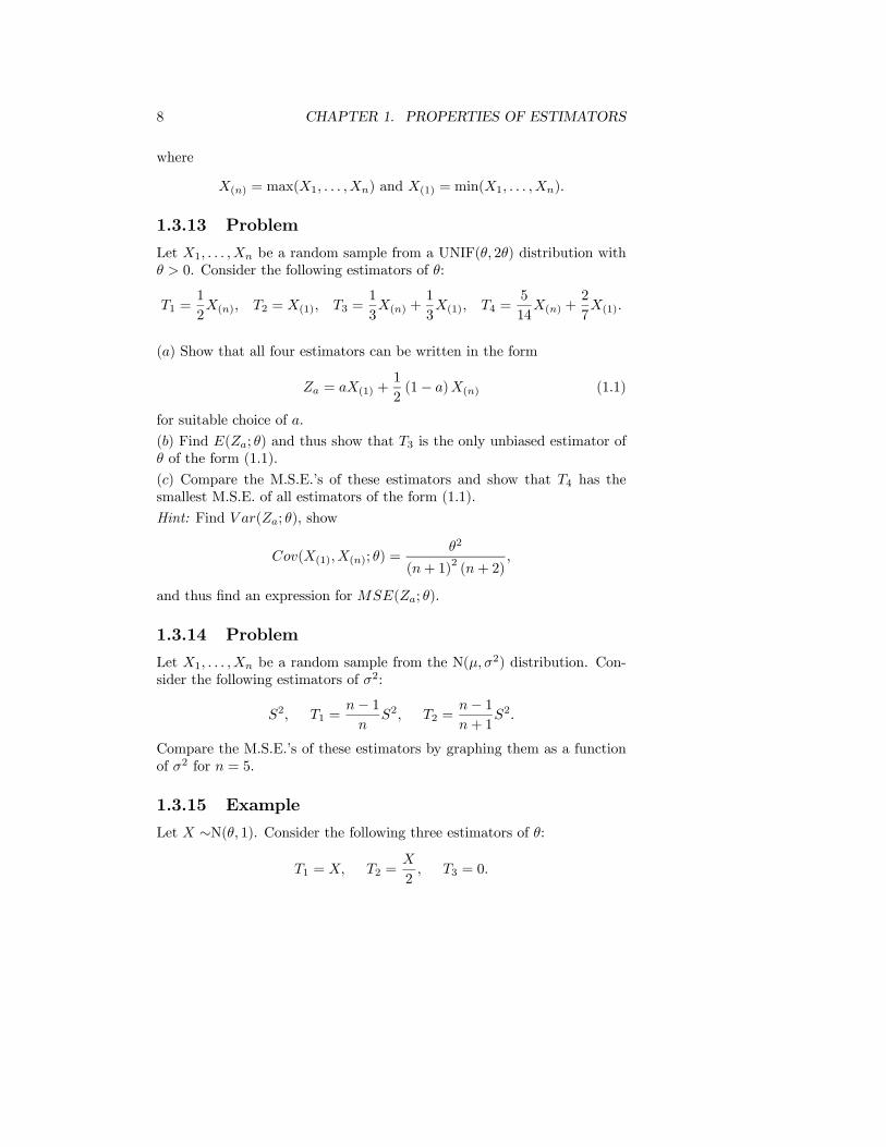
1.3.13 Problem
Let X1, . . . ,Xn be a random sample from a UNIF(θ, 2θ) distribution withθ > 0. Consider the following estimators of θ:
T1 =1
2X(n), T2 = X(1), T3 =
1
3X(n) +
1
3X(1), T4 =
5
14X(n) +
2
7X(1).
(a) Show that all four estimators can be written in the form
Za = aX(1) +1
2(1− a)X(n) (1.1)
for suitable choice of a.
(b) Find E(Za; θ) and thus show that T3 is the only unbiased estimator ofθ of the form (1.1).
(c) Compare the M.S.E.’s of these estimators and show that T4 has thesmallest M.S.E. of all estimators of the form (1.1).
Hint: Find V ar(Za; θ), show
Cov(X(1),X(n); θ) =θ2
(n+ 1)2 (n+ 2),
and thus find an expression for MSE(Za; θ).
1.3.14 Problem
Let X1, . . . ,Xn be a random sample from the N(μ,σ2) distribution. Con-sider the following estimators of σ2:
S2, T1 =n− 1n
S2, T2 =n− 1n+ 1
S2.
Compare the M.S.E.’s of these estimators by graphing them as a functionof σ2 for n = 5.
1.3.15 Example
Let X ∼N(θ, 1). Consider the following three estimators of θ:
T1 = X, T2 =X
2, T3 = 0.
1.3. UNBIASEDNESS AND MEAN SQUARE ERROR 9
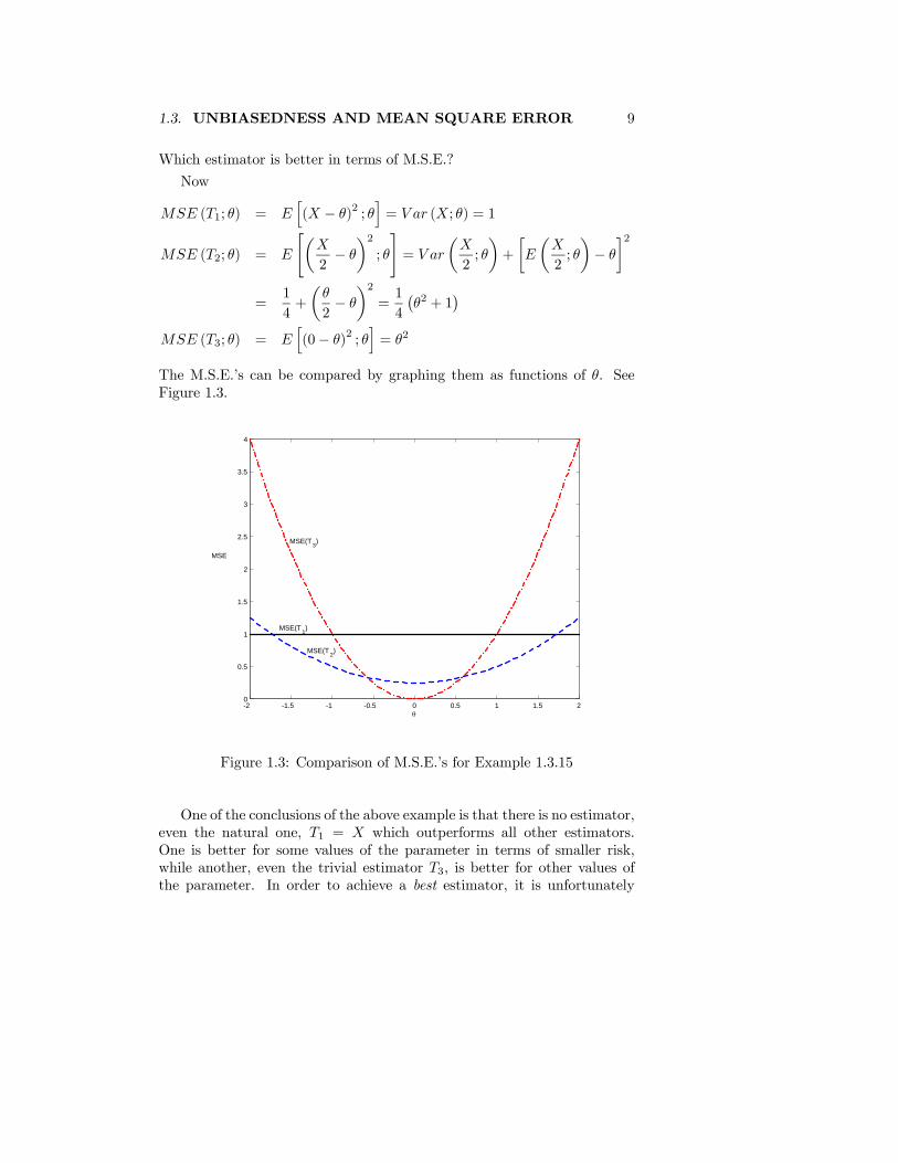
Which estimator is better in terms of M.S.E.?
Now
MSE (T1; θ) = Eh(X − θ)2 ; θ
i= V ar (X; θ) = 1
MSE (T2; θ) = E
"µX
2− θ
¶2; θ
#= V ar
µX
2; θ
¶+
∙E
µX
2; θ
¶− θ
¸2=
1
4+
µθ
2− θ
¶2=1
4
¡θ2 + 1
¢MSE (T3; θ) = E
h(0− θ)
2; θi= θ2
The M.S.E.’s can be compared by graphing them as functions of θ. SeeFigure 1.3.
-2 -1.5 -1 -0.5 0 0.5 1 1.5 20
0.5
1
1.5
2
2.5
3
3.5
4
θ
MSE
MSE(T 1)
MSE(T 2)
MSE(T 3)
Figure 1.3: Comparison of M.S.E.’s for Example 1.3.15
One of the conclusions of the above example is that there is no estimator,even the natural one, T1 = X which outperforms all other estimators.One is better for some values of the parameter in terms of smaller risk,while another, even the trivial estimator T3, is better for other values ofthe parameter. In order to achieve a best estimator, it is unfortunately
10 CHAPTER 1. PROPERTIES OF ESTIMATORS
necessary to restrict ourselves to a specific class of estimators and selectthe best within the class. Of course, the best within this class will only beas good as the class itself, and therefore we must ensure that restrictingourselves to this class is sensible and not unduly restrictive. The class ofall estimators is usually too large to obtain a meaningful solution. Onepossible restriction is to the class of all unbiased estimators.
1.3.16 Definition
An estimator T = T (X) is said to be a uniformly minimum variance un-biased estimator (U.M.V.U.E.) of the parameter θ if (i) it is an unbiasedestimator of θ and (ii) among all unbiased estimators of θ it has the smallestM.S.E. and therefore the smallest variance.
1.3.17 Problem
Suppose X has a GAM(2, θ) distribution and consider the class of estima-tors aX; a ∈ <+. Find the estimator in this class which minimizes themean absolute error for estimating the scale parameter θ. Hint: Show
E (|aX − θ|; θ) = θE (|aX − 1|; θ = 1) .
Is this estimator unbiased? Is it the best estimator in the class of allfunctions of X?
1.4 Sufficiency
A sufficient statistic is one that, from a certain perspective, contains all thenecessary information for making inferences about the unknown parame-ters in a given model. By making inferences we mean the usual conclusionsabout parameters such as estimators, significance tests and confidence in-tervals.Suppose the data are X and T = T (X) is a sufficient statistic. The
intuitive basis for sufficiency is that ifX has a conditional distribution givenT (X) that does not depend on θ, then X is of no value in addition to T inestimating θ. The assumption is that random variables carry information ona statistical parameter θ only insofar as their distributions (or conditionaldistributions) change with the value of the parameter. All of this, of course,assumes that the model is correct and θ is the only unknown. It shouldbe remembered that the distribution of X given a sufficient statistic Tmay have a great deal of value for some other purpose, such as testing thevalidity of the model itself.
1.4. SUFFICIENCY 11
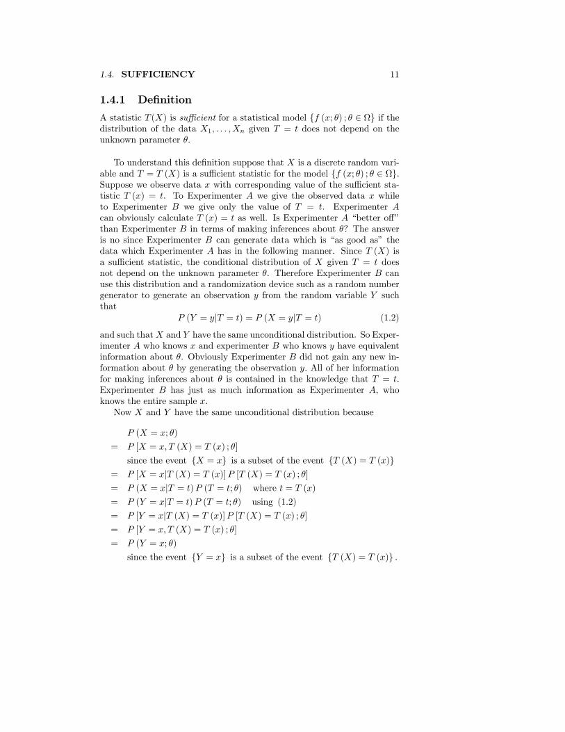
1.4.1 Definition
A statistic T (X) is sufficient for a statistical model f (x; θ) ; θ ∈ Ω if thedistribution of the data X1, . . . ,Xn given T = t does not depend on theunknown parameter θ.
To understand this definition suppose that X is a discrete random vari-able and T = T (X) is a sufficient statistic for the model f (x; θ) ; θ ∈ Ω.Suppose we observe data x with corresponding value of the sufficient sta-tistic T (x) = t. To Experimenter A we give the observed data x whileto Experimenter B we give only the value of T = t. Experimenter Acan obviously calculate T (x) = t as well. Is Experimenter A “better off”than Experimenter B in terms of making inferences about θ? The answeris no since Experimenter B can generate data which is “as good as” thedata which Experimenter A has in the following manner. Since T (X) isa sufficient statistic, the conditional distribution of X given T = t doesnot depend on the unknown parameter θ. Therefore Experimenter B canuse this distribution and a randomization device such as a random numbergenerator to generate an observation y from the random variable Y suchthat
P (Y = y|T = t) = P (X = y|T = t) (1.2)
and such thatX and Y have the same unconditional distribution. So Exper-imenter A who knows x and experimenter B who knows y have equivalentinformation about θ. Obviously Experimenter B did not gain any new in-formation about θ by generating the observation y. All of her informationfor making inferences about θ is contained in the knowledge that T = t.Experimenter B has just as much information as Experimenter A, whoknows the entire sample x.Now X and Y have the same unconditional distribution because
P (X = x; θ)
= P [X = x, T (X) = T (x) ; θ]
since the event X = x is a subset of the event T (X) = T (x)= P [X = x|T (X) = T (x)]P [T (X) = T (x) ; θ]= P (X = x|T = t)P (T = t; θ) where t = T (x)
= P (Y = x|T = t)P (T = t; θ) using (1.2)
= P [Y = x|T (X) = T (x)]P [T (X) = T (x) ; θ]= P [Y = x, T (X) = T (x) ; θ]
= P (Y = x; θ)
since the event Y = x is a subset of the event T (X) = T (x) .
12 CHAPTER 1. PROPERTIES OF ESTIMATORS
The use of a sufficient statistic is formalized in the following principle:
1.4.2 The Sufficiency Principle
Suppose T (X) is a sufficient statistic for a model f (x; θ) ; θ ∈ Ω. Supposex1, x2 are two different possible observations that have identical values ofthe sufficient statistic:
T (x1) = T (x2).
Then whatever inference we would draw from observing x1 we should drawexactly the same inference from x2.
If we adopt the sufficiency principle then we partition the sample space(the set of all possible outcomes) into mutually exclusive sets of outcomesin which all outcomes in a given set lead to the same inference about θ.This is referred to as data reduction.
1.4.3 Example
Let (X1, . . . ,Xn) be a random sample from the POI(θ) distribution. Show
that T =nPi=1Xi is a sufficient statistic for this model.
1.4.4 Problem
Let X1, . . . ,Xn be a random sample from the Bernoulli(θ) distribution and
let T =nPi=1Xi.
(a) Find the conditional distribution of (X1, . . . ,Xn) given T = t and thusshow T is a sufficient statistic for this model.
(b) Explain how you would generate data with the same distribution as theoriginal data using the value of the sufficient statistic and a randomizationdevice.
(c) Let U = U(X1) = 1 if X1 = 1 and 0 otherwise. Find E(U) andE(U |T = t).
1.4.5 Problem
Let X1, . . . ,Xn be a random sample from the GEO(θ) distribution and let
T =nPi=1Xi.
1.4. SUFFICIENCY 13
(a) Find the conditional distribution of (X1, . . . ,Xn) given T = t and thusshow T is a sufficient statistic for this model.
(b) Explain how you would generate data with the same distribution as theoriginal data using the value of the sufficient statistic and a randomizationdevice.
(d) Find E(X1|T = t).
1.4.6 Problem
Let X1, . . . ,Xn be a random sample from the EXP(1, θ) distribution andlet T = X(1).
(a) Find the conditional distribution of (X1, . . . ,Xn) given T = t and thusshow T is a sufficient statistic for this model.
(b) Explain how you would generate data with the same distribution as theoriginal data using the value of the sufficient statistic and a randomizationdevice.
(c) Find E [(X1 − 1) ; θ] and E [(X1 − 1) |T = t].
1.4.7 Problem
Let X1, . . . ,Xn be a random sample from the distribution with probabilitydensity function f (x; θ) . Show that the order statisticT (X) = (X(1), . . . ,X(n)) is sufficient for the model f (x; θ) ; θ ∈ Ω.
The following theorem gives a straightforward method for identifyingsufficient statistics.
1.4.8 Factorization Criterion for Sufficiency
Suppose X has probability (density) function f (x; θ) ; θ ∈ Ω and T (X)is a statistic. Then T (X) is a sufficient statistic for f (x; θ) ; θ ∈ Ω if andonly if there exist two non—negative functions g(.) and h(.) such that
f (x; θ) = g(T (x); θ)h(x), for all x, θ ∈ Ω.
Note that this factorization need only hold on a set A of possible values ofX which carries the full probability, that is,
f (x; θ) = g(T (x); θ)h(x), for all x ∈ A, θ ∈ Ω
where P (X ∈ A; θ) = 1, for all θ ∈ Ω.
14 CHAPTER 1. PROPERTIES OF ESTIMATORS
Note that the function g(T (x); θ) depends on both the parameter θ andthe sufficient statistic T (X) while the function h(x) does not depend onthe parameter θ.
1.4.9 Example
Let X1, . . . ,Xn be a random sample from the N(μ,σ2) distribtion. Show
that (nPi=1Xi,
nPi=1X2i ) is a sufficient statistic for this model. Show that
(X, S2) is also a sufficient statistic for this model.
1.4.10 Example
Let X1, . . . ,Xn be a random sample from the WEI(1, θ) distribution. Finda sufficient statistic for this model.
1.4.11 Example
LetX1, . . . ,Xn be a random sample from the UNIF(0, θ) distribution. Showthat T = X(n) is a sufficient statistic for this model. Find the conditionalprobability density function of (X1, . . . ,Xn) given T = t.
1.4.12 Problem
Let X1, . . . ,Xn be a random sample from the EXP(1, θ) distribution. Showthat X(1) is a sufficient statistic for this model and find the conditionalprobability density function of (X1, . . . ,Xn) given X(1) = t.
1.4.13 Problem
Use the Factorization Criterion for Sufficiency to show that if T (X) isa sufficient statistic for the model f (x; θ) ; θ ∈ Ω then any one-to-onefunction of T is also a sufficient statistic.
We have seen above that sufficient statistics are not unique. One-to-one functions of a statistic contain the same information as the originalstatistic. Fortunately, we can characterise all one-to-one functions of astatistic in terms of the way in which they partition the sample space. Notethat the partition induced by the sufficient statistic provides a partition ofthe sample space into sets of observations which lead to the same inferenceabout θ. See Figure 1.4.
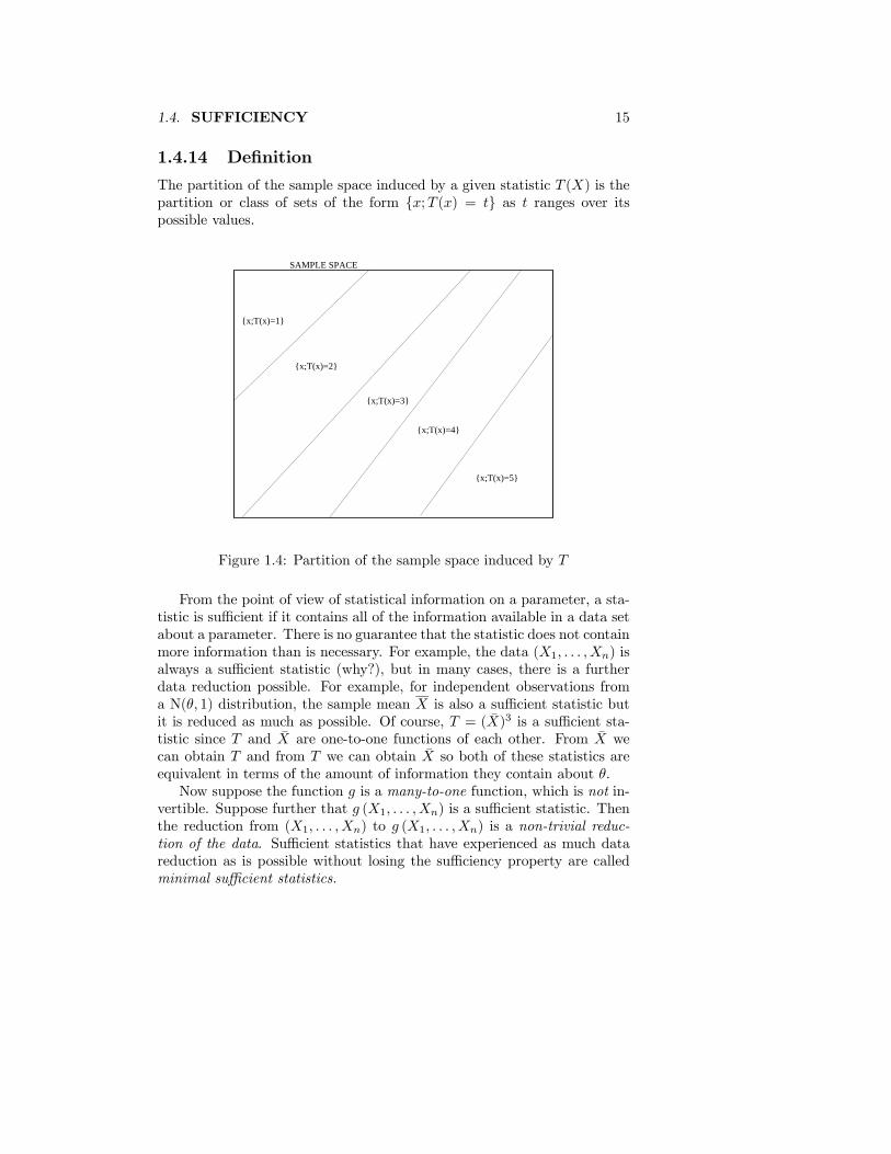
1.4. SUFFICIENCY 15
1.4.14 Definition
The partition of the sample space induced by a given statistic T (X) is thepartition or class of sets of the form x;T (x) = t as t ranges over itspossible values.
SAMPLE SPACE
x;T(x)=5
x;T(x)=1
x;T(x)=2
x;T(x)=3
x;T(x)=4
Figure 1.4: Partition of the sample space induced by T
From the point of view of statistical information on a parameter, a sta-tistic is sufficient if it contains all of the information available in a data setabout a parameter. There is no guarantee that the statistic does not containmore information than is necessary. For example, the data (X1, . . . ,Xn) isalways a sufficient statistic (why?), but in many cases, there is a furtherdata reduction possible. For example, for independent observations froma N(θ, 1) distribution, the sample mean X is also a sufficient statistic butit is reduced as much as possible. Of course, T = (X)3 is a sufficient sta-tistic since T and X are one-to-one functions of each other. From X wecan obtain T and from T we can obtain X so both of these statistics areequivalent in terms of the amount of information they contain about θ.Now suppose the function g is a many-to-one function, which is not in-
vertible. Suppose further that g (X1, . . . ,Xn) is a sufficient statistic. Thenthe reduction from (X1, . . . ,Xn) to g (X1, . . . ,Xn) is a non-trivial reduc-tion of the data. Sufficient statistics that have experienced as much datareduction as is possible without losing the sufficiency property are calledminimal sufficient statistics.
16 CHAPTER 1. PROPERTIES OF ESTIMATORS
1.5 Minimal Sufficiency
Now we wish to consider those circumstances under which a given statistic(actually the partition of the sample space induced by the given statistic)allows no further real reduction. Suppose g(.) is a many-to-one functionand hence is a real reduction of the data. Is g(T ) still sufficient? In somecases, as in the example below, the answer is “no”.
1.5.1 Problem
Let X1, . . . ,Xn be a random sample from the Bernoulli(θ) distribution.
Show that T (X) =nPi=1Xi is sufficient for this model. Show that if g is not
a one-to-one function, (g(t1) = g(t2) = g0 for some integers t1 and t2 where0 ≤ t1 < t2 ≤ n) then g(T ) cannot be sufficient for f (x; θ) ; θ ∈ Ω.Hint: Find P (T = t1|g(T ) = g0).
1.5.2 Definition
A statistic T (X) is a minimal sufficient statistic for f (x; θ) ; θ ∈ Ω if itis sufficient and if for any other sufficient statistic U(X), there exists afunction g(.) such that T (X) = g(U(X)).
This definition says that a minimal sufficient statistic is a function ofevery other sufficient statistic. In terms of the partition induced by theminimal sufficient this implies that the minimal sufficient statistic inducesthe coarsest partition possible of the sample space among all sufficientstatistics. This partition is called the minimal sufficient partition.
1.5.3 Problem
Prove that if T1 and T2 are both minimal sufficient statistics, then theyinduce the same partition of the sample space.
The following theorem is useful in showing a statistic is minimally suf-ficient.
1.5. MINIMAL SUFFICIENCY 17
1.5.4 Theorem - Minimal Sufficient Statistic
Suppose the model is f (x; θ) ; θ ∈ Ω and let A = support of X. PartitionA into the equivalence classes defined by
Ay =½x;f (x; θ)
f(y; θ)= H(x, y) for all θ ∈ Ω
¾, y ∈ A.
This is a minimal sufficient partition. The statistic T (X) which inducesthis partition is a minimal sufficient statistic.
The proof of this theorem is given in Section 5.4.2 of the Ap-pendix.
1.5.5 Example
Let (X1, . . . ,Xn) be a random sample from the distribution with probabilitydensity function
f (x; θ) = θxθ−1, 0 < x < 1, θ > 0.
Find a minimal sufficient statistic for the model f (x; θ) ; θ ∈ Ω.
1.5.6 Example
Let X1, . . . ,Xn be a random sample from the N(θ, θ2) distribution. Find aminimal sufficient statistic for the model f (x; θ) ; θ ∈ Ω.
1.5.7 Problem
LetX1, . . . ,Xn be a random sample from the LOG(1, θ) distribution. Provethat the order statistic (X(1), . . . ,X(n)) is a minimal sufficient statistic forthe model f (x; θ) ; θ ∈ Ω.
1.5.8 Problem
Let X1, . . . ,Xn be a random sample from the CAU(1, θ) distribution. Finda minimal sufficient statistic for the model f (x; θ) ; θ ∈ Ω.
1.5.9 Problem
Let X1, . . . ,Xn be a random sample from the UNIF(θ, θ + 1) distribution.Find a minimal sufficient statistic for the model f (x; θ) ; θ ∈ Ω.
18 CHAPTER 1. PROPERTIES OF ESTIMATORS
1.5.10 Problem
Let Ω denote the set of all probability density functions. Let (X1, . . . ,Xn)be a random sample from a distribution with probability density functionf ∈ Ω. Prove that the order statistic (X(1), . . . ,X(n)) is a minimal suffi-cient statistic for the model f(x); f ∈ Ω. Note that in this example theunknown “parameter” is f .
1.5.11 Problem - Linear Regression
Suppose E(Y ) = Xβ where Y = (Y1, . . . , Yn)T is a vector of independent
and normally distributed random variables with V ar(Yi) = σ2, i = 1, . . . , n,X is a n× k matrix of known constants of rank k and β = (β1, . . . ,βk)
T isa vector of unknown parameters. Let
β =¡XTX
¢−1XTY and S2e = (Y −Xβ)T (Y −Xβ)/(n− k).
Show that (β, S2e ) is a minimal sufficient statistic for this model.Hint: Show
(Y −Xβ)T (Y −Xβ) = (n− k)S2e + (β − β)TXTX(β − β).
1.6 Completeness
The property of completeness is one which is useful for determining theuniqueness of estimators, for verifying, in some cases, that a minimal suffi-cient statistic has been found, and for finding U.M.V.U.E.’s.
Let X1, . . . ,Xn denote the observations from a distribution with proba-bility (density) function f (x; θ) ; θ ∈ Ω. Suppose T (X) is a statistic andu(T ), a function of T , is an unbiased estimator of θ so that E[u(T ); θ] = θfor all θ ∈ Ω. Under what circumstances is this the only unbiased esti-mator which is a function of T? To answer this question, suppose u1(T )and u2(T ) are both unbiased estimators of θ and consider the differenceh(T ) = u1(T ) − u2(T ). Since u1(T ) and u2(T ) are both unbiased estima-tors we have E[h(T ); θ] = 0 for all θ ∈ Ω. Now if the only function h(T )which satisfies E[h(T ); θ] = 0 for all θ ∈ Ω is the function h(t) = 0, then thetwo unbiased estimators must be identical. A statistic T with this propertyis said to be complete. The property of completeness is really a property ofthe family of distributions of T generated as θ varies.
1.6. COMPLETENESS 19
1.6.1 Definition
The statistic T = T (X) is a complete statistic for f (x; θ) ; θ ∈ Ω if
E[h(T ); θ] = 0, for all θ ∈ Ω
implies
P [h(T ) = 0; θ] = 1 for all θ ∈ Ω.
1.6.2 Example
LetX1, . . . ,Xn be a random sample from the N(θ, 1) distribution. Consider
T = T (X) = (X1,nPi=2Xi). Prove that T is a sufficient statistic for the model
f (x; θ) ; θ ∈ Ω but not a complete statistic.
1.6.3 Example
Let X1, . . . ,Xn be a random sample from the Bernoulli(θ) distribution.
Prove that T = T (X) =nPi=1Xi is a complete sufficient statistic for the
model f (x; θ) ; θ ∈ Ω.
1.6.4 Example
LetX1, . . . ,Xn be a random sample from the UNIF(0, θ) distribution. Showthat T = T (X) = X(n) is a complete statistic for the modelf (x; θ) ; θ ∈ Ω.
1.6.5 Problem
Prove that any one-to-one function of a complete sufficient statistic is acomplete sufficient statistic.
1.6.6 Problem
Let X1, . . . ,Xn be a random sample from the N(θ, aθ2) distribution wherea > 0 is a known constant and θ > 0. Show that the minimal sufficientstatistic is not a complete statistic.
20 CHAPTER 1. PROPERTIES OF ESTIMATORS
1.6.7 Theorem
If T (X) is a complete sufficient statistic for the model f (x; θ) ; θ ∈ Ωthen T (X) is a minimal sufficient statistic for f (x; θ) ; θ ∈ Ω.
The proof of this theorem is given in Section 5.4.3 of the Ap-pendix.
1.6.8 Problem
The converse to the above theorem is not true. Let X1, . . . ,Xn be arandom sample from the UNIF(θ − 1, θ + 1) distribution. Show that T =T (X) = (X(1),X(n)) is a minimal sufficient statistic for the model. Showalso that for the non-zero function
h(T ) =X(n) −X(1)
2− n− 1n+ 1
,
E[h(T ); θ] = 0 for all θ ∈ Ω and therefore T is not a complete statistic.
1.6.9 Example
Let X = X1, . . . ,Xn be a random sample from the UNIF(0, θ) distribu-tion. Prove that T = T (X) = X(n) is a minimal sufficient statistic forf (x; θ) ; θ ∈ Ω.
1.6.10 Problem
Let X = X1, . . . ,Xn be a random sample from the EXP(1, θ) distribu-tion. Prove that T = T (X) = X(1) is a minimal sufficient statistic forf (x; θ) ; θ ∈ Ω.
1.6.11 Theorem
For any random variables X and Y ,
E(X) = E[E(X|Y )]
and
V ar(X) = E[V ar(X|Y )] + V ar[E(X|Y )]
1.6. COMPLETENESS 21
1.6.12 Theorem
If T = T (X) is a complete statistic for the model f (x; θ) ; θ ∈ Ω, thenthere is at most one function of T that provides an unbiased estimator ofthe parameter τ(θ).
1.6.13 Problem
Prove Theorem 1.6.12.
1.6.14 Theorem (Lehmann-Scheffe)
If T = T (X) is a complete sufficient statistic for the model f (x; θ) ; θ ∈ Ωand E [g (T ) ; θ] = τ(θ), then g(T ) is the unique U.M.V.U.E. of τ(θ).
1.6.15 Example
Let X1, . . . ,Xn be a random sample from the Bernoulli(θ) distribution.Find the U.M.V.U.E. of τ(θ) = θ2.
1.6.16 Example
Let X1, . . . ,Xn be a random sample from the UNIF(0, θ) distribution. Findthe U.M.V.U.E. of τ(θ) = θ.
1.6.17 Problem
Let X1, . . . ,Xn be a random sample from the Bernoulli(θ) dsitribution.Find the U.M.V.U.E. of τ(θ) = θ(1− θ).
1.6.18 Problem
Suppose X has a Hypergeometric distribution with p.f.
f (x; θ) =
µNθ
x
¶µN −Nθ
n− x
¶µN
n
¶ , x = 0, 1, . . . ,min (Nθ, N −Nθ) ;
θ ∈ Ω =
½0,1
N,2
N, . . . , 1
¾Show that X is a complete sufficient statistic. Find the U.M.V.U.E. of θ.

22 CHAPTER 1. PROPERTIES OF ESTIMATORS
1.6.19 Problem
Let X1, . . . ,Xn be a random sample from the EXP(β,μ) distribution whereβ is known. Show that T = X(1) is a complete sufficient statistic for thismodel. Find the U.M.V.U.E. of μ and the U.M.V.U.E. of μ2.
1.6.20 Problem
Suppose X1, ...,Xn is a random sample from the UNIF(a, b) distribution.Show that T = (X(1),X(n)) is a complete sufficient statistic for this model.Find the U.M.V.U.E.’s of a and b. Find the U.M.V.U.E. of the mean of Xi.
1.6.21 Problem
Let T (X) be an unbiased estimator of τ(θ). Prove that T (X) is a U.M.V.U.E.of τ(θ) if and only if E(UT ; θ) = 0 for all U(X) such that E(U) = 0 for allθ ∈ Ω.
1.6.22 Theorem (Rao-Blackwell)
If T = T (X) is a complete sufficient statistic for the model f (x; θ) ; θ ∈ Ωand U = U(X) is any unbiased estimator of τ(θ), then E(U |T ) is theU.M.V.U.E. of τ(θ).
1.6.23 Problem
Let X1, . . . ,Xn be a random sample from the EXP(β,μ) distribution whereβ is known. Find the U.M.V.U.E. of τ (μ) = P (X1 > c;μ) where c ∈ < isa known constant. Hint: Let U = U(X1) = 1 if X1 ≥ c and 0 otherwise.
1.6.24 Problem
Let X1, . . . ,Xn be a random sample from the DU(θ) distribution. Showthat T = X(n) is a complete sufficient statistic for this model. Find theU.M.V.U.E. of θ.
1.7. THE EXPONENTIAL FAMILY 23
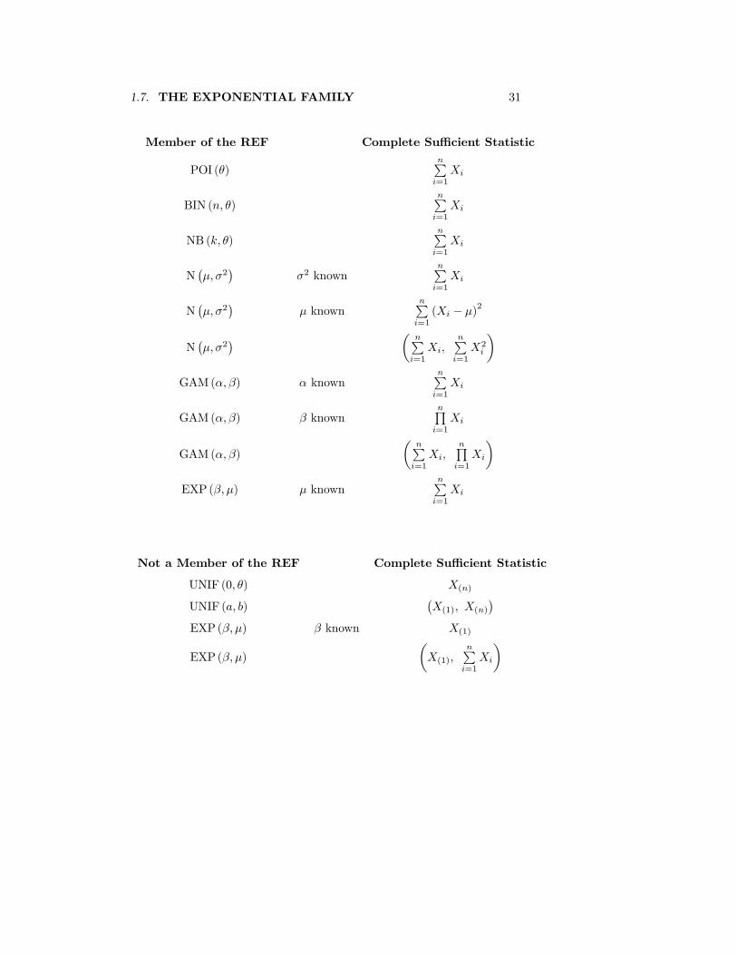
1.7 The Exponential Family
1.7.1 Definition
Suppose X = (X1, . . . ,Xp) has a (joint) probability (density) function ofthe form
f (x; θ) = C(θ) exp
"kPj=1
qj(θ)Tj(x)
#h(x) (1.3)
for functions qj(θ), Tj(x), h(x), C(θ). Then we say that f (x; θ) is a mem-ber of the exponential family of densities. We call (T1(X), . . . , Tk(X)) thenatural sufficient statistic.
It should be noted that the natural sufficient statistic is not unique.Multiplication of Tj by a constant and division of qj by the same constantresults in the same function f (x; θ). More generally linear transformationsof the Tj and the qj can also be used.
1.7.2 Example
Prove that T (X) = (T1(X), . . . , Tk(X)) is a sufficient statistic for the modelf (x; θ) ; θ ∈ Ω where f (x; θ) has the form (1.3).
1.7.3 Example
Show that the BIN(n, θ) distribution has an exponential family distributionand find the natural sufficient statistic.
One of the important properties of the exponential family is its closureunder repeated independent sampling.
1.7.4 Theorem
Let X1, . . . ,Xn be a random sample from the distribution with probability(density) function given by (1.3). Then (X1, . . . ,Xn) also has an exponen-tial family form, with joint probability (density) function
f(x1, . . . xn; θ) = [C (θ)]n exp
(kPj=1
qj (θ)
∙nPi=1Tj (xi)
¸)nQi=1h (xi) .
24 CHAPTER 1. PROPERTIES OF ESTIMATORS
In other words, C is replaced by Cn and Tj(x) bynPi=1Tj(xi). The natural
sufficient statistic is µnPi=1T1(Xi), . . . ,
nPi=1Tk(Xi)
¶.
1.7.5 Example
Let X1, . . . ,Xn be a random sample from the POI(θ) distribution. Showthat X1, . . . ,Xn is a member of the exponential family.
1.7.6 Canonical Form of the Exponential Family
It is usual to reparameterize equation (1.3) by replacing qj(θ) by a newparameter ηj . This results in the canonical form of the exponential family
f(x; η) = C(η) exp
"kPj=1
ηjTj(x)
#h(x).
The natural parameter space in this form is the set of all values of η forwhich the above function is integrable; that is
η;∞Z−∞
f(x; η)dx <∞.
If X is discrete the intergral is replaced by the sum over all x such thatf(x; η) > 0.
If the statistic satisfies a linear constraint, for example,
P
ÃkPj=1
Tj(X) = 0; η
!= 1,
then the number of terms k can be reduced. Unless this is done, the pa-rameters ηj are not all statistically meaningful. For example the data maypermit us to estimate η1+η2 but not allow estimation of η1 and η2 individ-ually. In this case we call the parameter “unidentifiable”. We will need toassume that the exponential family representation is minimal in the sensethat neither the ηj nor the Tj satisfy any linear constraints.
1.7. THE EXPONENTIAL FAMILY 25
1.7.7 Definition
We will say that X has a regular exponential family distribution if it is incanonical form, is of full rank in the sense that neither the Tj nor the ηjsatisfy any linear constraints, and the natural parameter space contains ak−dimensional rectangle. By Theorem 1.7.4 if Xi has a regular exponentialfamily distribution then X = (X1, . . . ,Xn) also has a regular exponentialfamily distribution.
1.7.8 Example
Show that X ∼ BIN(n, θ) has a regular exponential family distribution.
1.7.9 Theorem
If X has a regular exponential family distribution with natural sufficientstatistic T (X) = (T1(X), . . . , Tk(X)) then T (X) is a complete sufficientstatistic. Reference: Lehmann and Ramano (2005), Testing StatisticalHypotheses (3rd edition), pp. 116-117.
1.7.10 Differentiating under the Integral
In Chapter 2, it will be important to know if a family of models has theproperty that differentiation under the integral is possible. We state thatfor a regular exponential family, it is possible to differentiate under theintegral, that is,
∂m
∂ηmi
ZC(η) exp
"kPj=1
ηjTj(x)
#h(x)dx =
Z∂m
∂ηmiC(η) exp
"kPj=1
ηjTj(x)
#h(x)dx
for any m = 1, 2, . . . and any η in the interior of the natural parameterspace.
1.7.11 Example
Let X1, . . . ,Xn be a random sample from the N(μ,σ2) distribution. Finda complete sufficient statistic for this model. Find the U.M.V.U.E.’s of μand σ2.
1.7.12 Example
Show that X ∼ N(θ, θ2) does not have a regular exponential family distri-bution.
26 CHAPTER 1. PROPERTIES OF ESTIMATORS
1.7.13 Example
Suppose (X1,X2,X3) have joint density
f (x1, x2, x3; θ1, θ2, θ3) = P (X1 = x1,X2 = x2,X3 = x3; θ1, θ2, θ3)
=n!
x1!x2!x3!θx11 θx22 θx33
xi = 0, 1, . . . ; i = 1, 2, 3; x1 + x2 + x3 = n
0 < θi < 1; i = 1, 2, 3; θ1 + θ2 + θ3 = 1
Find the U.M.V.U.E. of θ1, θ2, and θ1θ2.
Since
f (x1, x2, x3; θ1, θ2, θ3) = exp
"3Pj=1
qj (θ1, θ2, θ3)Tj (x1, x2, x3)
#h (x1, x2, x3)
where
qj (θ1, θ2, θ3) = log θj , Tj (x1, x2, x3) = xj , j = 1, 2, 3 and h (x1, x2, x3) =n!
x1!x2!x3!,
(X1,X2,X3) is a member of the exponential family. But
3Pj=1
Tj (x1, x2, x3) = n and θ1 + θ2 + θ3 = 1
and thus (X1,X2,X3) is not a member of the regular exponential family.However by substituting X3 = n −X1 −X2 and θ3 = 1 − θ1 − θ2 we canshow that (X1,X2) has a regular exponential family distribution.Let
η1 = log
µθ1
1− θ1 − θ2
¶, η2 = log
µθ2
1− θ1 − θ2
¶then
θ1 =eη1
1 + eη1 + eη2, θ2 =
eη2
1 + eη1 + eη2.
LetT1 (x1, x2) = x1, T2 (x1, x2) = x2,
C (η1, η2) =
µ1
1 + eη1 + eη2
¶n, and h (x1, x2) =
n!
x1!x2! (n− x1 − x2)!.
In canonical form (X1,X2) has p.f.
f (x1, x2; η1, η2) = C (η1, η2) exp [η1T1 (x1, x2) + η2T2 (x1, x2)]h (x1, x2)
1.7. THE EXPONENTIAL FAMILY 27
with natural parameter space (η1, η2) ; η1 ∈ <, η2 ∈ < which contains atwo-dimensional rectangle. The η0js and the T
0js do not satisfy any linear
constraints. Therefore (X1,X2) has a regular exponential family distri-bution with natural sufficient statistic T (X1,X2) = (X1,X2) and thusT (X1,X2) is a complete sufficient statistic.By the properties of the multinomial distribution (see Section 5.2.2)
we have X1 v BIN (n, θ1) , X2 v BIN (n, θ2) and Cov (X1,X2) = −nθ1θ2.Since
E
µX1n; θ1, θ2
¶=nθ1n= θ1 and E
µX2n; θ1, θ2
¶=nθ2n= θ2
then by the Lehmann-Scheffe Theorem X1/n is the U.M.V.U.E. of θ1 andX2/n is the U.M.V.U.E. of θ2.Since
−nθ1θ2 = Cov (X1,X2; θ1, θ2)
= E (X1X2; θ1, θ2)− E (X1; θ1, θ2)E (X2; θ1, θ2)= E (X1X2; θ1, θ2)− n2θ1θ2
or
E
µX1X2n (n− 1) ; θ1, θ2
¶= θ1θ2
then by the Lehmann-Scheffe TheoremX1X2/ [n (n− 1)] is the U.M.V.U.E.of θ1θ2.
1.7.14 Example
Let X1, . . . ,Xn be a random sample from the POI(θ) distribution. Find theU.M.V.U.E. of τ(θ) = e−θ. Show that the U.M.V.U.E. is also a consistentestimator of τ(θ).
Since (X1, . . . ,Xn) is a member of the regular exponential family with
natural sufficient statistic T =nPi=1Xi therefore T is a complete sufficient
statistic. Consider the random variable U(X1) = 1 if X1 = 0 and 0 other-wise. Then
E [U(X1); θ] = 1 · P (X1 = 0; θ) = e−θ, θ > 0
and U(X1) is an unbiased estimator of τ(θ) = e−θ. Therefore by the Rao-
Blackwell Theorem E (U |T ) is the U.M.V.U.E. of τ(θ) = e−θ.
28 CHAPTER 1. PROPERTIES OF ESTIMATORS
Since X1, . . . ,Xn is a random sample from the POI(θ) distribution,
X1 v POI (θ) , T =nPi=1Xi v POI (nθ) and
nPi=2Xi v POI ((n− 1) θ) .
Thus
E (U |T = t) = 1 · P (X1 = 0|T = t)
=
P
µX1 = 0,
nPi=1Xi = t; θ
¶P (T = t; θ)
=
P
µX1 = 0,
nPi=2Xi = t− 0; θ
¶P (T = t; θ)
= e−θ[(n− 1) θ]t e−(n−1)θ
t!÷ (nθ)
t
t!e−nθ
=
µ1− 1
n
¶t, t = 0, 1, . . .
Therefore E (U |T ) =¡1− 1
n
¢Tis the U.M.V.U.E. of θ.
Since X1, . . . ,Xn is a random sample from the POI(θ) distribution thenby the W.L.L.N. X →p θ and by the Limit Theorems (see Section 5.3)
E (U |T ) =µ1− 1
n
¶T=
∙µ1− 1
n
¶n¸X→p e
−θ
and therefore E (U |T ) a consistent estimator of e−θ.
1.7.15 Example
Let X1, . . . ,Xn be a random sample from the N(θ, 1) distribution. Find theU.M.V.U.E. of τ(θ) = Φ(c − θ) = P (Xi ≤ c; θ) for some constant c whereΦ is the standard normal cumulative distribution function. Show that theU.M.V.U.E. is also a consistent estimator of τ(θ).
Since (X1, . . . ,Xn) is a member of the regular exponential family with
natural sufficient statistic T =nPi=1Xi therefore T is a complete sufficient
statistic. Consider the random variable U(X1) = 1 if X1 ≤ c and 0 other-wise. Then
E [U(X1); θ] = 1 · P (X1 ≤ c; θ) = Φ(c− θ), θ ∈ <
1.7. THE EXPONENTIAL FAMILY 29
and U(X1) is an unbiased estimator of τ(θ) = Φ(c− θ). Therefore by theRao-Blackwell Theorem E (U |T ) is the U.M.V.U.E. of τ(θ) = Φ(c− θ).Since X1, . . . ,Xn is a random sample from the N(θ, 1) distribution,
X1 v N(θ, 1), T =nPi=1Xi v N(nθ, n) and
nPi=2Xi v N((n− 1) θ, n− 1).
The conditional p.d.f. of X1 given T = t is
f (x1|T = t)
=1√2πexp
∙−12(x1 − θ)2
¸× 1p
2π (n− 1)exp
(− [t− x1 − (n− 1) θ]
2
2 (n− 1)
)÷ 1√
2πnexp
(− [t− nθ]
2
2n
)
=1q
2π¡1− 1
n
¢ exp(−12
"x21 +
(t− x1)2
n− 1 − t2
n
#)
=1q
2π¡1− 1
n
¢ exp"− 1
2¡1− 1
n
¢ µx1 − t
n
¶2#
which is the p.d.f. of a N( tn , 1−1n) random variable. Since X1|T = t has a
N( tn , 1−1n) distribution,
E (U |T ) = 1 · P (X1 ≤ c|T )
= Φ
⎛⎝ c− T/nq¡1− 1
n
¢⎞⎠
is the U.M.V.U.E. of τ(θ) = Φ(c− θ).Since X1, . . . ,Xn is a random sample from the N(θ, 1) distribution then
by the W.L.L.N. X →p θ and by the Limit Theorems
E (U |T ) = Φ
⎛⎝ c− T/nq¡1− 1
n
¢⎞⎠ = Φ
⎛⎝ c− Xq¡1− 1
n
¢⎞⎠→p Φ (c− θ)
and therefore E (U |T ) a consistent estimator τ(θ) = Φ(c− θ).
30 CHAPTER 1. PROPERTIES OF ESTIMATORS
1.7.16 Problem
Let X1, . . . ,Xn be a random sample from the distribution with probabilitydensity function
f (x; θ) = θxθ−1, 0 < x < 1, θ > 0.
Show that the geometric mean of the sample
µnQi=1Xi
¶1/nis a complete
sufficient statistic and find the U.M.V.U.E. of θ.
Hint: − logXi ∼ EXP(1/θ).
1.7.17 Problem
Let X1, . . . ,Xn be a random sample from the EXP(β,μ) distribution where
μ is known. Show that T =nPi=1Xi is a complete sufficient statistic. Find
the U.M.V.U.E. of β2.
1.7.18 Problem
Let X1, . . . ,Xn be a random sample from the GAM(α,β) distribution andθ = (α,β). Find the U.M.V.U.E. of τ(θ) = αβ.
1.7.19 Problem
Let X ∼ NB(k, θ). Find the U.M.V.U.E. of θ.Hint: Find E[(X + k − 1)−1; θ].
1.7.20 Problem
Let X1, . . . ,Xn be a random sample from the N(θ, 1) distribution. Findthe U.M.V.U.E. of τ(θ) = θ2.
1.7.21 Problem
Let X1, . . . ,Xn be a random sample from the N(0, θ) distribution. Findthe U.M.V.U.E. of τ(θ) = θ2.
1.7.22 Problem
Let X1, . . . ,Xn be a random sample from the POI(θ) distribution. Findthe U.M.V.U.E. for τ(θ) = (1 + θ)e−θ.
Hint: Find P (X1 ≤ 1; θ).
1.7. THE EXPONENTIAL FAMILY 31
Member of the REF Complete Sufficient Statistic
POI (θ)nPi=1Xi
BIN (n, θ)nPi=1Xi
NB(k, θ)nPi=1Xi
N¡μ,σ2
¢σ2 known
nPi=1Xi
N¡μ,σ2
¢μ known
nPi=1(Xi − μ)2
N¡μ,σ2
¢ µnPi=1Xi,
nPi=1X2i
¶GAM(α,β) α known
nPi=1Xi
GAM(α,β) β knownnQi=1Xi
GAM(α,β)
µnPi=1Xi,
nQi=1Xi
¶EXP (β,μ) μ known
nPi=1Xi
Not a Member of the REF Complete Sufficient Statistic
UNIF (0, θ) X(n)
UNIF (a, b)¡X(1), X(n)
¢EXP(β,μ) β known X(1)
EXP(β,μ)
µX(1),
nPi=1Xi
32 CHAPTER 1. PROPERTIES OF ESTIMATORS
1.7.23 Problem
Let X1, . . . ,Xn be a random sample form the POI(θ) distribution. Findthe U.M.V.U.E. for τ(θ) = e−2θ. Hint: Find E[(−1)X1 ; θ] . Show that thisestimator has some undesirable properties when n = 1 and n = 2 but whenn is large, it is approximately equal to the maximum likelihood estimator.
1.7.24 Problem
Let X1, . . . ,Xn be a random sample from the GAM(2, θ) distribution. Findthe U.M.V.U.E. of τ1(θ) = 1/θ and the U.M.V.U.E. ofτ2(θ) = P (X1 > c; θ) where c > 0 is a constant.
1.7.25 Problem
In Problem 1.5.11 show that β is the U.M.V.U.E. of β and S2e is theU.M.V.U.E. of σ2.
1.7.26 Problem
A Brownian Motion process is a continuous-time stochastic process X (t)which is often used to describe the value of an asset. Assume X (t) rep-resents the market price of a given asset such as a portfolio of stocks attime t and x0 is the value of the portfolio at the beginning of a given timeperiod (assume that the analysis is conditional on x0 so that x0 is fixedand known). The distribution of X (t) for any fixed time t is assumed to beN(x0+μt,σ2t) for 0 < t ≤ 1. The parameter μ is the drift of the Brownianmotion process and the parameter σ is the diffusion coefficient. Assumethat t = 1 corresponds to the end of the time period so X (1) is the closingprice.Suppose that we record both the period high max
0≤t≤1X (t) and the close
X (1). Define random variables
M = max0≤t≤1
X (t)− x0
andY = X (1)− x0.
The joint probability density function of (M,Y ) can be shown to be
f(m, y;μ,σ2) =2 (2m− y)√
2πσ3exp
½1
2σ2
h2μy − μ2 − (2m− y)2
i¾,
m > 0, −∞ < y < m, μ ∈ < and σ2 > 0.
1.8. ANCILLARITY 33
(a) Show that (M,Y ) has a regular exponential family distribution.
(b) Let Z = M(M − Y ). Show that Y v N¡μ,σ2
¢and Z v EXP
¡σ2/2
¢independently.
(c) Suppose we record independent pairs of observations (Mi, Yi),i = 1, . . . n on the portfolio for a total of n distinct time periods. Find theU.M.V.U.E.’s of μ and σ2.
(d) Show that the estimators
V1 =1
n− 1nPi=1
¡Yi − Y
¢2and
V2 =2
n
nPi=1Zi =
2
n
nPi=1Mi (Mi − Yi)
are also unbiased estimators of σ2. How do we know that neither of theseestimators is the U.M.V.U.E. of σ2? Show that the U.M.V.U.E. of σ2 canbe written as a weighted average of V1 and V2. Compare the variances ofall three estimators.
(e) An up-and-out call option on the portfolio is an option with exerciseprice ξ (a constant) which pays a total of (X (1)− ξ) dollars at the end ofone period provided that this quantity is positive and provided that X (t)never exceeded the value of a barrier throughout this period of time, thatis, provided that M < a. Thus the option pays
g(M,Y ) = max Y − (ξ − x0), 0 if M < a
and otherwise g(M,Y ) = 0. Find the expected value of such an option,that is, find the expected value of g(M,Y ).
1.8 Ancillarity
Let X = (X1, . . . ,Xn) denote observations from a distribution with proba-bility (density) function f (x; θ) ; θ ∈ Ω and let U(X) be a statistic. Theinformation on the parameter θ is provided by the sensitivity of the distri-bution of a statistic to changes in the parameter. For example, suppose amodest change in the parameter value leads to a large change in the ex-pected value of the distribution resulting in a large shift in the data. Thenthe parameter can be estimated fairly precisely. On the other hand, if astatistic U has no sensitivity at all in distribution to the parameter, thenit would appear to contain little information for point estimation of thisparameter. A statistic of the second kind is called an ancillary statistic.

34 CHAPTER 1. PROPERTIES OF ESTIMATORS
1.8.1 Definition
U(X) is an ancillary statistic if its distribution does not depend on theunknown parameter θ.
Ancillary statistics are, in a sense, orthogonal or perpendicular to mini-mal sufficient statistics. Ancillary statistics are analogous to the residuals ina multiple regression, while the complete sufficient statistics are analogousto the estimators of the regression coefficients. It is well-known that theresiduals are uncorrelated with the estimators of the regression coefficients(and independent in the case of normal errors). However, the “irrelevance”of the ancillary statistic seems to be limited to the case when it is not partof the minimal (preferably complete) sufficient statistic as the followingexample illustrates.
1.8.2 Example
Suppose a fair coin is tossed to determine a random variable N = 1 withprobability 1/2 and N = 100 otherwise. We then observe a Binomial ran-dom variable X with parameters (N, θ). Show that the minimal sufficientstatistic is (X,N) but that N is an ancillary statistic. Is N irrelevant toinference about θ?
In this example it seems reasonable to condition on an ancillary compo-nent of the minimal sufficient statistic. Conducting inference conditionallyon the ancillary statistic essentially means treating the observed number oftrials as if it had been fixed in advance instead of the result of the toss ofa fair coin. This example also illustrates the use of the following principle:
1.8.3 The Conditionality Principle
Suppose the minimal sufficient statistic can be written in the formT = (U,A) where A is an ancillary statistic. Then all inference should beconducted using the conditional distribution of the data given the value ofthe ancillary statistic, that is, using the distribution of X|A.
Some difficulties arise from the application of this principle since thereis no general method for constructing the ancillary statistic and ancillarystatistics are not necessarily unique.
1.8. ANCILLARITY 35
The following theorem allows us to use the properties of completenessand ancillarity to prove the independence of two statistics without findingtheir joint distribution.
1.8.4 Basu’s Theorem
Consider X with probability (density) function f (x; θ) ; θ ∈ Ω. Let T (X)be a complete sufficient statistic. Then T (X) is independent of every an-cillary statistic U(X).
1.8.5 Proof
We need to show
P [U(X) ∈ B,T (X) ∈ C; θ] = P [U(X) ∈ B; θ] · P [T (X) ∈ C; θ]
for all sets B,C and all θ ∈ Ω.Let
g(t) = P [U(X) ∈ B|T (X) = t]− P [U(X) ∈ B]
for all t ∈ A where P (T ∈ A; θ) = 1. By sufficiency, P [U(X) ∈ B|T (X) = t]does not depend on θ, and by ancillarity, P [U(X) ∈ B] also does notdepend on θ. Therefore g(T ) is a statistic.Let
IU(X) ∈ B =½
1 if U(X) ∈ B0 else.
ThenE[IU(X) ∈ B] = P [U(X) ∈ B],
E[IU(X) ∈ B|T = t] = P [U(X) ∈ B|T = t],
andg(t) = E[IU(X) ∈ B|T (X) = t]−E[IU(X) ∈ B].
This gives
E[g(T )] = E[E[IU(X) ∈ B|T ]]−E[IU(X) ∈ B]= E[IU(X) ∈ B]−E[IU(X) ∈ B]= 0 for all θ ∈ Ω,
and since T is complete this implies P [g(T ) = 0; θ] = 1 for all θ ∈ Ω.Therefore
P [U(X) ∈ B|T (X) = t] = P [U(X) ∈ B] for all t ∈ A and all B. (1.4)
36 CHAPTER 1. PROPERTIES OF ESTIMATORS
Suppose T has probability density function h(t; θ). Then
P [U(X) ∈ B,T (X) ∈ C; θ] =ZC
P [U(X) ∈ B|T = t]h(t; θ)dt
=
ZC
P [U(X) ∈ B]h(t; θ)dt by (1.4)
= P [U(X) ∈ B] ·ZC
h(t; θ)dt
= P [U(X) ∈ B] · P [T (X) ∈ C; θ]
true for all sets B,C and all θ ∈ Ω as required.¥
1.8.6 Example
Let X1, . . . ,Xn be a random sample from the EXP(θ) distribution. Show
that T (X1, . . . ,Xn) =nPi=1
Xi and U(X1, . . . ,Xn) = (X1/T, . . . ,Xn/T ) are
independent random variables. Find E(X1/T ).
1.8.7 Example
Let X1, . . . ,Xn be a random sample from the N(μ,σ2) distribution. Provethat X and S2 are independent random variables.
1.8.8 Problem
Let X1, . . . ,Xn be a random sample from the distribution with p.d.f.
f (x;β) =2x
β2, 0 < x ≤ β.
(a) Show that β is a scale parameter for this model.
(b) Show that T = T (X1, . . . ,Xn) = X(n) is a complete sufficient statisticfor this model.
(c) Find the U.M.V.U.E. of β.
(d) Show that T and U = U (X) = X1/T are independent random variables.
(e) Find E (X1/T ).
1.8. ANCILLARITY 37
1.8.9 Problem
Let X1, . . . ,Xn be a random sample from the GAM(α,β) distribution.
(a) Show that β is a scale parameter for this model.
(b) Suppose α is known. Show that T = T (X1, . . . ,Xn) =nPi=1Xi is a
complete sufficient statistic for the model.
(c) Show that T and U = U(X1, . . . ,Xn) = (X1/T, . . . ,Xn/T ) are inde-pendent random variables.
(d) Find E(X1/T ).
1.8.10 Problem
In Problem 1.5.11 show that β and S2e are independent random variables.
1.8.11 Problem
Let X1, . . . ,Xn be a random sample from the EXP(β,μ) distribution.
(a) Suppose β is known. Show that T1 = X(1) is a complete sufficientstatistic for the model.
(b) Show that T1 and T2 =nPi=1
¡Xi −X(1)
¢are independent random vari-
ables.
(c) Find the p.d.f. of T2. Hint: Show
nPi=1(Xi − μ) = n (T1 − μ) + T2.
(d) Show that (T1, T2) is a complete sufficient statistic for the modelf (x1, . . . , xn;μ,β) ;μ ∈ <, β > 0.(e) Find the U.M.V.U.E.’s of β and μ.
38 CHAPTER 1. PROPERTIES OF ESTIMATORS
1.8.12 Problem
Let X1, . . . ,Xn be a random sample from the distribution with p.d.f.
f (x;α,β) =αxα−1
βα, α > 0, 0 < x ≤ β.
(a) Show that if α is known then T1 = X(n) is a complete sufficient statisticfor the model.
(b) Show that T1 and T2 =nQi=1
Xi
T1are independent random variables.
(c) Find the p.d.f. of T2. Hint: Show
nXi=1
log
µXiβ
¶= log T2 + n log
µT1β
¶.
(d) Show that (T1, T2) is a complete sufficient statistic for the model.
(e) Find the U.M.V.U.E. of α.
Chapter 2
Maximum LikelihoodEstimation
2.1 Maximum Likelihood Method- One Parameter
Suppose we have collected the data x (possibly a vector) and we believe thatthese data are observations from a distribution with probability function
P (X = x; θ) = f(x; θ)
where the scalar parameter θ is unknown and θ ∈ Ω. The probability ofobserving the data x is equal to f(x; θ). When the observed value of x issubstituted into f(x; θ), then f(x; θ) is a function of the parameter θ only.In the absence of any other information, it seems logical that we shouldestimate the parameter θ using a value most compatible with the data. Forexample we might choose the value of θ which maximizes the probabilityof the observed data.
2.1.1 Definition
Suppose X is a random variable with probability functionP (X = x; θ) = f(x; θ), where θ ∈ Ω is a scalar and suppose x is the ob-served data. The likelihood function for θ is
L(θ) = P (observing the data x; θ)
= P (X = x; θ)
= f(x; θ), θ ∈ Ω.
39
40 CHAPTER 2. MAXIMUM LIKELIHOOD ESTIMATION
If X = (X1, . . . ,Xn) is a random sample from the probability functionP (X = x; θ) = f(x; θ) and x = (x1, . . . , xn) are the observed data then thelikelihood function for θ is
L(θ) = P (observing the data x; θ)
= P (X1 = x1, . . . ,Xn = xn; θ)
=nQi=1f(xi; θ), θ ∈ Ω.
The value of θ which maximizes the likelihood L (θ) also maximizesthe logarithm of the likelihood function. (Why?) Since it is easier to findthe derivative of the sum of n terms rather than the product, we usuallydetermine the maximum of the logarithm of the likelihood function.
2.1.2 Definition
The log likelihood function is defined as
l(θ) = logL(θ), θ ∈ Ω
where log is the natural logarithmic function.
2.1.3 Definition
The value of θ that maximizes the likelihood function L(θ) or equivalentlythe log likelihood function l(θ) is called the maximum likelihood (M.L.)estimate. The M.L. estimate is a function of the data x and we writeθ = θ (x). The corresponding M.L. estimator is denoted θ = θ(X).
2.1.4 Example
Suppose in a sequence of n Bernoulli trials with P (Success) = θ we haveobserved x successes. Find the likelihood function L (θ), the log likelihoodfunction l (θ), the M.L. estimate of θ and the M.L. estimator of θ.
2.1.5 Example
Suppose we have collected data x1, . . . , xn and we believe these observa-tions are independent observations from a POI(θ) distribution. Find thelikelihood function, the log likelihood function, the M.L. estimate of θ andthe M.L. estimator of θ.
2.1. MAXIMUMLIKELIHOODMETHOD- ONE PARAMETER 41
2.1.6 Problem
Suppose we have collected data x1, . . . , xn and we believe these observa-tions are independent observations from the DU(θ) distribution. Find thelikelihood function, the M.L. estimate of θ and the M.L. estimator of θ.
2.1.7 Definition
The score function is defined as
S(θ) =d
dθl (θ) =
d
dθlogL (θ) , θ ∈ Ω.
2.1.8 Definition
The information function is defined as
I(θ) = − d2
dθ2l(θ) = − d
2
dθ2logL(θ), θ ∈ Ω.
I(θ) is called the observed information.
In Section 2.7 we will see how the observed information I(θ) can be usedto construct approximate confidence intervals for the unknown parameterθ. I(θ) also tells us about the concavity of the log likelihood function.
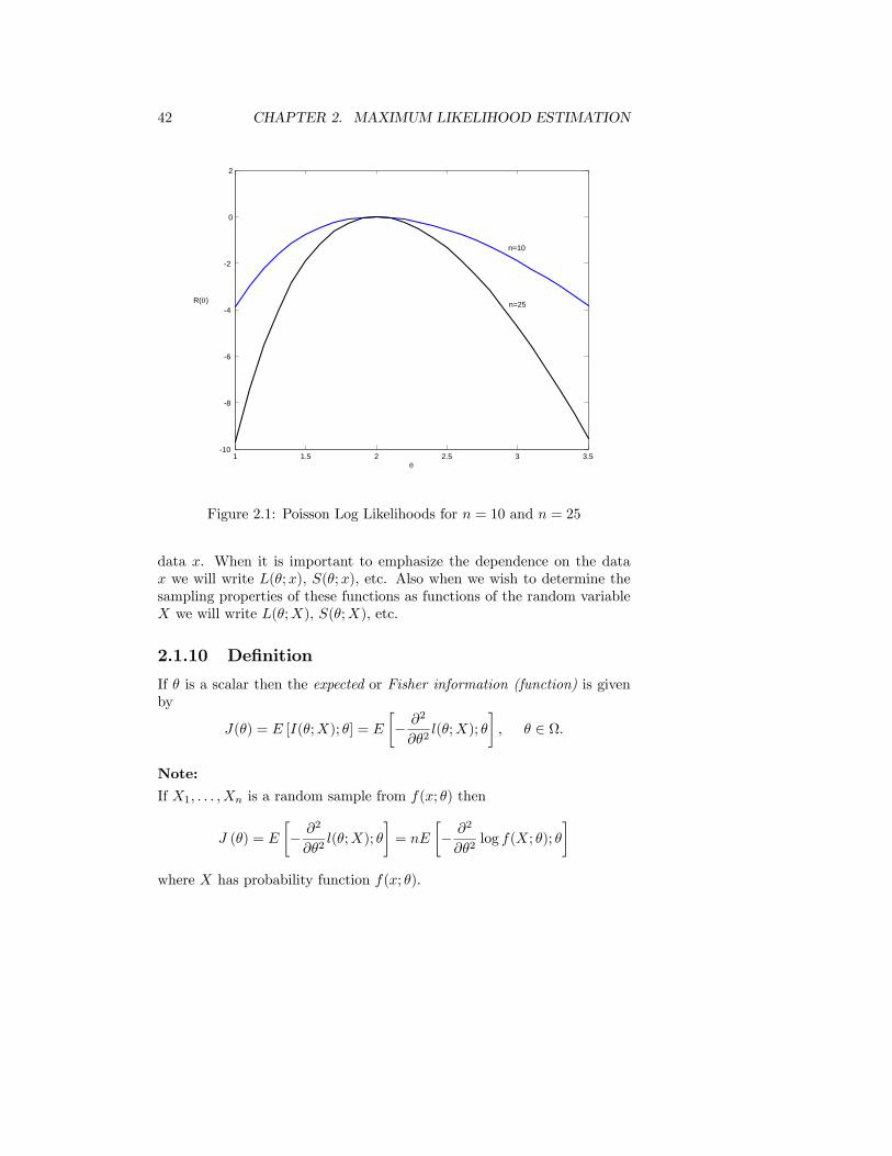
Suppose in Example 2.1.5 the M.L. estimate of θ was θ = 2. If n = 10then I(θ) = 10/2 = 5. If n = 25 then I(θ) = 25/2 = 12.5. See Figure2.1. The log likelihood function is more concave down for n = 25 than forn = 10 which reflects the fact that as the number of observations increaseswe have more “information” about the unknown parameter θ.
2.1.9 Finding M.L. Estimates
IfX1, . . . ,Xn is a random sample from a distribution whose support set doesnot depend on θ then we usually find θ by solving S(θ) = 0. It is important
to verify that θ is the value of θ which maximizes L (θ) or equivalently l (θ).This can be done using the First Derivative Test. Note that the conditionI(θ) > 0 only checks for a local maximum.
Although we view the likelihood, log likelihood, score and information func-tions as functions of θ they are, of course, also functions of the observed
42 CHAPTER 2. MAXIMUM LIKELIHOOD ESTIMATION
1 1.5 2 2.5 3 3.5-10
-8
-6
-4
-2
0
2
θ
R(θ)
n=10
n=25
Figure 2.1: Poisson Log Likelihoods for n = 10 and n = 25
data x. When it is important to emphasize the dependence on the datax we will write L(θ;x), S(θ;x), etc. Also when we wish to determine thesampling properties of these functions as functions of the random variableX we will write L(θ;X), S(θ;X), etc.
2.1.10 Definition
If θ is a scalar then the expected or Fisher information (function) is givenby
J(θ) = E [I(θ;X); θ] = E
∙− ∂2
∂θ2l(θ;X); θ
¸, θ ∈ Ω.
Note:
If X1, . . . ,Xn is a random sample from f(x; θ) then
J (θ) = E
∙− ∂2
∂θ2l(θ;X); θ
¸= nE
∙− ∂2
∂θ2log f(X; θ); θ
¸where X has probability function f(x; θ).
2.1. MAXIMUMLIKELIHOODMETHOD- ONE PARAMETER 43
2.1.11 Example
Find the Fisher information based on a random sampleX1, . . . ,Xn from thePOI(θ) distribution and compare it to the variance of the M.L. estimator
θ. How does the Fisher information change as n increases?
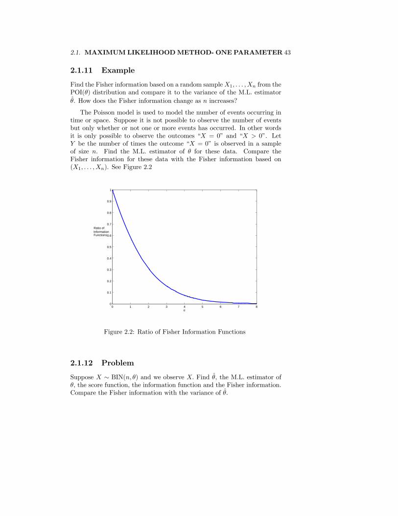
The Poisson model is used to model the number of events occurring intime or space. Suppose it is not possible to observe the number of eventsbut only whether or not one or more events has occurred. In other wordsit is only possible to observe the outcomes “X = 0” and “X > 0”. LetY be the number of times the outcome “X = 0” is observed in a sampleof size n. Find the M.L. estimator of θ for these data. Compare theFisher information for these data with the Fisher information based on(X1, . . . ,Xn). See Figure 2.2
0 1 2 3 4 5 6 7 80
0.1
0.2
0.3
0.4
0.5
0.6
0.7
0.8
0.9
1
θ
Ratio ofInformationFunctions
Figure 2.2: Ratio of Fisher Information Functions
2.1.12 Problem
Suppose X ∼ BIN(n, θ) and we observe X. Find θ, the M.L. estimator ofθ, the score function, the information function and the Fisher information.Compare the Fisher information with the variance of θ.
44 CHAPTER 2. MAXIMUM LIKELIHOOD ESTIMATION
2.1.13 Problem
Suppose X ∼ NB(k, θ) and we observe X. Find the M.L. estimator of θ,the score function and the Fisher information.
2.1.14 Problem - Randomized Sampling
A professor is interested estimating the unknown quantity θ which is theproportion of students who cheat on tests. She conducts an experiment inwhich each student is asked to toss a coin secretly. If the coin comes up ahead the student is asked to toss the coin again and answer “Yes” if thesecond toss is a head and “No” if the second toss is a tail. If the first tossof the coin comes up a tail, the student is asked to answer “Yes” or “No”to the question: Have you ever cheated on a University test? Studentsare assumed to answer more honestly in this type of randomized responsesurvey because it is not known to the questioner whether the answer “Yes”is a result of tossing the coin twice and obtaining two heads or because thestudent obtained a tail on the toss of the coin and then answered “Yes” tothe question about cheating.
(a) Find the probability that x students answer “Yes” in a class of n stu-dents.
(b) Find the M.L. estimator of θ based on X students answering “Yes” ina class of n students. Be sure to verify that your answer corresponds to amaximum.
(c) Find the Fisher information for θ.
(d) In a simpler experiment n students could be asked to answer “Yes”or “No” to the question: Have you ever cheated on a University test? Ifwe could assume that they answered the question honestly then we wouldexpect to obtain more information about θ from this simpler experiment.Determine the amount of information lost in doing the randomized responseexperiment as compared to the simpler experiment.
2.1.15 Problem
Suppose (X1,X2) ∼ MULT(n, θ2, 2θ (1− θ)). Find the M.L. estimator ofθ, the score function and the Fisher information.
2.1.16 Likelihood Functions for Continuous Models
Suppose X is a continuous random variable with probability density func-tion f(x; θ). We will often observe only the value of X rounded to some
2.1. MAXIMUMLIKELIHOODMETHOD- ONE PARAMETER 45
degree of precision (say one decimal place) in which case the actual obser-vation is a discrete random variable. For example, suppose we observe Xcorrect to one decimal place. Then
P (we observe 1.1) =
1.15Z1.05
f(x; θ)dx ≈ (1.15− 1.05) · f(1.1; θ)
assuming the function f(x; θ) is quite smooth over the interval. More gen-erally, if we observe X rounded to the nearest ∆ (assumed small) then thelikelihood of the observation is approximately ∆f(observation; θ). Sincethe precision ∆ of the observation does not depend on the parameter, thenmaximizing the discrete likelihood of the observation is essentially equiva-lent to maximizing the probability density function f(observation; θ) overthe parameter.Therefore if X = (X1, . . . ,Xn) is a random sample from the probability
density function f(x; θ) and x = (x1, . . . , xn) are the observed data thenwe define the likelihood function for θ as
L(θ) = L (θ;x) =nQi=1f(xi; θ), θ ∈ Ω.
See also Problem 2.8.12.
2.1.17 Example
Suppose X1, . . . ,Xn is a random sample from the distribution with proba-bility density function
f(x; θ) = θxθ−1, 0 ≤ x ≤ 1, θ > 0.
Find the score function, the M.L. estimator, and the information functionof θ. Find the observed information. Find the mean and variance of θ.Compare the Fisher infomation and the variance of θ.
2.1.18 Example
Suppose X1, . . . ,Xn is a random sample from the UNIF(0, θ) distribution.Find the M.L. estimator of θ.
2.1.19 Problem
Suppose X1, . . . ,Xn is a random sample from the UNIF(θ, θ + 1) distribu-tion. Show the M.L. estimator of θ is not unique.
46 CHAPTER 2. MAXIMUM LIKELIHOOD ESTIMATION
2.1.20 Problem
Suppose X1, . . . ,Xn is a random sample from the DE(1, θ) distribution.Find the M.L. estimator of θ.
2.1.21 Problem
Show that if θ is the unique M.L. estimator of θ then θ must be a functionof the minimal sufficient statistic.
2.1.22 Problem
The word information generally implies something that is additive. Sup-pose X has probability (density) function f (x; θ) , θ ∈ Ω and independentlyY has probability (density) function g(y; θ), θ ∈ Ω. Show that the Fisherinformation in the joint observation (X,Y ) is the sum of the Fisher infor-mation in X plus the Fisher information in Y .
Often S(θ) = 0 must be solved numerically using an iterative methodsuch as Newton’s Method.
2.1.23 Newton’s Method
Let θ(0) be an initial estimate of θ. We may update that value as follows:
θ(i+1) = θ(i) +S(θ(i))
I(θ(i)), i = 0, 1, . . .
Notes:
(1) The initial estimate, θ(0), may be determined by graphing L (θ) or l (θ).
(2) The algorithm is usually run until the value of θ(i) no longer changesto a reasonable number of decimal places. When the algorithm is stoppedit is always important to check that the value of θ obtained does indeedmaximize L (θ).
(3) This algorithm is also called the Newton-Raphson Method.
(4) I (θ) can be replaced by J (θ) for a similar algorithm which is called themethod of scoring or Fisher’s method of scoring.
(5) The value of θ may also be found by maximizing L(θ) or l(θ) usingthe maximization (minimization) routines available in various statisticalsoftware packages such as Maple, S-Plus, Matlab, R etc.
(6) If the support of X depends on θ (e.g. UNIF(0, θ)) then θ is not foundby solving S(θ) = 0.
2.1. MAXIMUMLIKELIHOODMETHOD- ONE PARAMETER 47
2.1.24 Example
Suppose X1, . . . ,Xn is a random sample from the WEI(1,β) distribution.Explain how you would find the M.L. estimate of β using Newton’s Method.How would you find the mean and variance of the M.L. estimator of β?
2.1.25 Problem - Likelihood Function for Grouped Data
Suppose X is a random variable with probability (density) function f (x; θ)and P (X ∈ A; θ) = 1. Suppose A1, A2, . . . , Am is a partition of A and let
pj(θ) = P (X ∈ Aj ; θ), j = 1, . . . ,m.
Suppose n independent observations are collected from this distribution butit is only possible to determine to which one of the m sets, A1, A2, . . . , Am,the i’th observation belongs. The observed data are:
Outcome A1 A2 ... Am TotalFrequency f1 f2 ... fm n
(a) Show that the Fisher information for these data is given by
J(θ) = nmPj=1
[p0j(θ)]2
pj(θ).
Hint: SincemPj=1
pj(θ) = 1,d
dθ
∙mPi=1pj(θ)
¸= 0.
(b) Explain how you would find the M.L. estimate of θ.
2.1.26 Definition
The relative likelihood function R(θ) is defined by
R(θ) = R (θ;x) =L(θ)
L(θ), θ ∈ Ω.
The relative likelihood function takes on values between 0 and 1.and canbe used to rank possible parameter values according to their plausibilitiesin light of the data. If R(θ1) = 0.1, say, then θ1 is rather an implausible
parameter value because the data are ten times more probable when θ = θthan they are when θ = θ1. However, if R(θ1) = 0.5, say, then θ1 is a fairlyplausible value because it gives the data 50% of the maximum possibleprobability under the model.
48 CHAPTER 2. MAXIMUM LIKELIHOOD ESTIMATION
2.1.27 Definition
The set of θ values for which R(θ) ≥ p is called a 100p% likelihood regionfor θ. If the region is an interval of real values then it is called a 100p%likelihood interval (L.I.) for θ.
Values inside the 10% L.I. are referred to as plausible and values outsidethis interval as implausible. Values inside a 50% L.I. are very plausible andoutside a 1% L.I. are very implausible in light of the data.
2.1.28 Definition
The log relative likelihood function is the natural logarithm of the relativelikelihood function:
r(θ) = r (θ;x) = log[R(θ)] = log[L(θ]− log[L(θ)] = l(θ)− l(θ), θ ∈ Ω.
Likelihood regions or intervals may be determined from a graph of R(θ)or r(θ) and usually it is more convenient to work with r(θ). Alternatively,they can be found by solving r(θ) − log p = 0. Usually this must be donenumerically.
2.1.29 Example
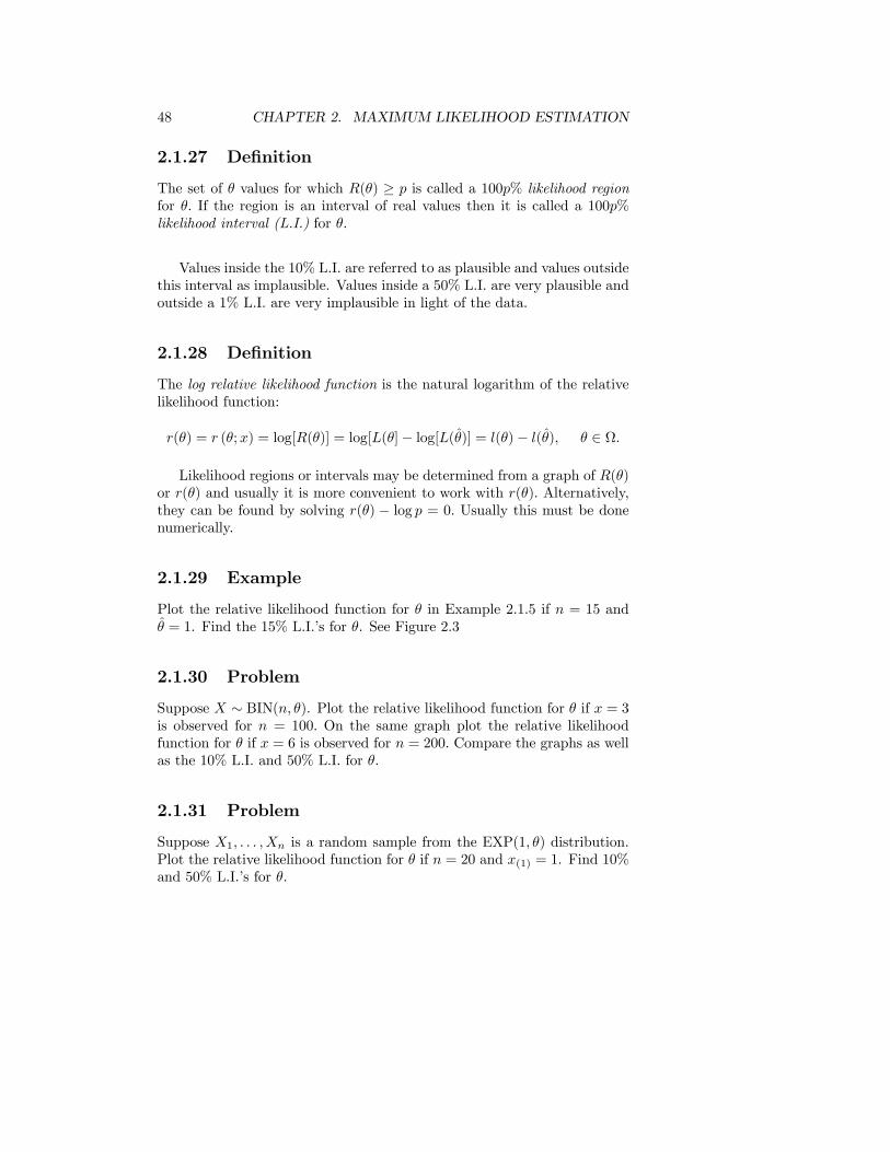
Plot the relative likelihood function for θ in Example 2.1.5 if n = 15 andθ = 1. Find the 15% L.I.’s for θ. See Figure 2.3
2.1.30 Problem
Suppose X ∼ BIN(n, θ). Plot the relative likelihood function for θ if x = 3is observed for n = 100. On the same graph plot the relative likelihoodfunction for θ if x = 6 is observed for n = 200. Compare the graphs as wellas the 10% L.I. and 50% L.I. for θ.
2.1.31 Problem
Suppose X1, . . . ,Xn is a random sample from the EXP(1, θ) distribution.Plot the relative likelihood function for θ if n = 20 and x(1) = 1. Find 10%and 50% L.I.’s for θ.
2.1. MAXIMUMLIKELIHOODMETHOD- ONE PARAMETER 49
0 0.5 1 1.5 2 2.50
0.1
0.2
0.3
0.4
0.5
0.6
0.7
0.8
0.9
1
θ
R(θ)
Figure 2.3: Relative Likelihood Function for Example 2.1.29
2.1.32 Problem
The following model is proposed for the distribution of family size in a largepopulation:
P (k children in family; θ) = θk, for k = 1, 2, . . .
P (0 children in family; θ) =1− 2θ1− θ
.
The parameter θ is unknown and 0 < θ < 12 . Fifty families were chosen at
random from the population. The observed numbers of children are givenin the following table:
No. of children 0 1 2 3 4 TotalFrequency observed 17 22 7 3 1 50
(a) Find the likelihood, log likelihood, score and information functions forθ.
50 CHAPTER 2. MAXIMUM LIKELIHOOD ESTIMATION
(b) Find the M.L. estimate of θ and the observed information.
(c) Find a 15% likelihood interval for θ.
(d) A large study done 20 years earlier indicated that θ = 0.45. Is thisvalue plausible for these data?
(e) Calculate estimated expected frequencies. Does the model give a rea-sonable fit to the data?
2.1.33 Problem
The probability that k different species of plant life are found in a randomlychosen plot of specified area is
pk (θ) =
¡1− e−θ
¢k+1(k + 1) θ
, k = 0, 1, . . . ; θ > 0.
The data obtained from an examination of 200 plots are given in the tablebelow:
No. of species 0 1 2 3 ≥ 4 TotalFrequency observed 147 36 13 4 0 200
(a) Find the likelihood, log likelihood, score and information functions forθ.
(b) Find the M.L. estimate of θ and the observed information.
(c) Find a 15% likelihood interval for θ.
(d) Is θ = 1 a plausible value of θ in light of the observed data?
(e) Calculate estimated expected frequencies. Does the model give a rea-sonable fit to the data?
2.2 Principles of Inference
In Chapter 1 we discussed the Sufficiency Principle and the ConditionalityPrinciple. There is another principle which is equivalent to the SufficiencyPrinciple. The likelihood ratios generate the minimal sufficient partition.In other words, two likelihood ratios will agree
f (x1; θ)
f (x1; θ0)=f (x2; θ)
f (x2; θ0)
if and only if the values of the minimal sufficient statistic agree, that is,T (x1) = T (x2). Thus we obtain:
2.2. PRINCIPLES OF INFERENCE 51
2.2.1 The Weak Likelihood Principle
Suppose for two different observations x1, x2, the likelihood ratios
f (x1; θ)
f (x1; θ0)=f (x2; θ)
f (x2; θ0)
for all values of θ, θ0 ∈ Ω. Then the two different observations x1, x2 shouldlead to the same inference about θ.
A weaker but similar principle, the Invariance Principle follows. Thiscan be used, for example, to argue that for independent identically dis-tributed observations, it is only the value of the observations (the orderstatistic) that should be used for inference, not the particular order inwhich those observations were obtained.
2.2.2 Invariance Principle
Suppose for two different observations x1, x2,
f (x1; θ) = f (x2; θ)
for all values of θ ∈ Ω. Then the two different observations x1, x2 shouldlead to the same inference about θ.
There are relationships among these and other principles. For exam-ple, Birnbaum proved that the Conditionality Principle and the SufficiencyPrinciple above imply a stronger version of a Likelihood Principle. How-ever, it is probably safe to say that while probability theory has been quitesuccessfully axiomatized, it seems to be difficult if not impossible to de-rive most sensible statistical procedures from a set of simple mathematicalaxioms or principles of inference.
2.2.3 Problem
Consider the model f (x; θ) ; θ ∈ Ω and suppose that θ is the M.L. esti-mator based on the observation X. We often draw conclusions about theplausibility of a given parameter value θ based on the relative likelihoodL(θ)
L(θ). If this is very small, for example, less than or equal to 1/N , we regard
the value of the parameter θ as highly unlikely. But what happens if thistest declares every value of the parameter unlikely?Suppose f (x; θ) = 1 if x = θ and f (x; θ) = 0 otherwise, where
θ = 1, 2, . . .N . Define f0(x) to be the discrete uniform distribution on the
52 CHAPTER 2. MAXIMUM LIKELIHOOD ESTIMATION
integers 1, 2, . . . , N. In this example the parameter space isΩ = θ; θ = 0, 1, ...,N. Show that the relative likelihood
f0 (x)
f (x; θ)≤ 1
N
no matter what value of x is observed. Should this be taken to mean thatthe true distribution cannot be f0?
2.3 Properties of the Score and Information- Regular Model
Consider the model f (x; θ) ; θ ∈ Ω. The following is a set of sufficientconditions which we will use to determine the properties of the M.L. es-timator of θ. These conditions are not the most general conditions butare sufficiently general for most applications. Notable exceptions are theUNIF(0, θ) and the EXP(1, θ) distributions which will be considered sepa-rately.For convenience we call a family of models which satisfy the following
conditions a regular family of distributions. (See 1.7.9.)
2.3.1 Regular Model
Consider the model f (x; θ) ; θ ∈ Ω. Suppose that:(R1) The parameter space Ω is an open interval in the real line.
(R2) The densities f (x; θ) have common support, so that the setA = x; f (x; θ) > 0 , does not depend on θ.
(R3) For all x ∈ A, f (x; θ) is a continuous, three times differentiable func-tion of θ.
(R4) The integralRA
f (x; θ) dx can be twice differentiated with respect to θ
under the integral sign, that is,
∂k
∂θk
ZA
f (x; θ) dx =
ZA
∂k
∂θkf (x; θ) dx, k = 1, 2 for all θ ∈ Ω.
(R5) For each θ0 ∈ Ω there exist a positive number c and function M (x)(both of which may depend on θ0), such that for all θ ∈ (θ0 − c, θ0 + c)¯
∂3 log f (x; θ)
∂θ3
¯< M(x)
2.3. PROPERTIES OF THE SCORE AND INFORMATION- REGULARMODEL53
holds for all x ∈ A, and
E [M (X) ; θ] <∞ for all θ ∈ (θ0 − c, θ0 + c) .
(R6) For each θ ∈ Ω,
0 < E
(∙∂2 log f (X; θ)
∂θ2
¸2; θ
)<∞
If these conditions hold with X a discrete random variable and theintegrals replaced by sums, then we shall also call this a regular family ofdistributions.
Condition (R3) insures that the function ∂ log f (x; θ) /∂θ has, for eachx ∈ A, a Taylor expansion as a function of θ.The following lemma provides one method of determining whether dif-
ferentiation under the integral sign (condition (R4)) is valid.
2.3.2 Lemma
Suppose ∂g (x; θ) /∂θ exists for all θ ∈ Ω, and all x ∈ A. Suppose also thatfor each θ0 ∈ Ω there exist a positive number c, and function G (x) (bothof which may depend on θ0), such that for all θ ∈ (θ0 − c, θ0 + c)¯
∂g (x; θ)
∂θ
¯< G(x)
holds for all x ∈ A, and ZA
G (x) dx <∞.
Then∂
∂θ
ZA
g(x, θ)dx =
ZA
∂
∂θg(x, θ)dx.
2.3.3 Theorem - Expectation and Variance of the ScoreFunction
If X = (X1, . . . ,Xn) is a random sample from a regular modelf (x; θ) ; θ ∈ Ω then
E[S(θ;X); θ] = 0
54 CHAPTER 2. MAXIMUM LIKELIHOOD ESTIMATION
and
V ar[S(θ;X); θ] = E[S(θ;X)]2; θ = E[I(θ;X); θ] = J(θ) <∞
for all θ ∈ Ω.
2.3.4 Problem - Invariance Property of M.L.Estimators
Suppose X1, . . . ,Xn is a random sample from a distribution with proba-bility (density) function f (x; θ) where f (x; θ) ; θ ∈ Ω is a regular family.Let S(θ) and J(θ) be the score function and Fisher information respectivelybased on X1, . . . ,Xn. Consider the reparameterization τ = h(θ) where his a one-to-one differentiable function with inverse function θ = g(τ). LetS∗(τ) and J∗(τ) be the score function and Fisher information respectivelyunder the reparameterization.(a) Show that τ = h(θ) is the M.L. estimator of τ where θ is the M.L.estimator of θ.
(b) Show that E[S∗(τ ;X); τ ] = 0 and J∗(τ) = [g0(τ)]2J [g(τ)].
2.3.5 Problem
It is natural to expect that if we compare the information available in theoriginal data X and the information available in some statistic T (X), thelatter cannot be greater than the former since T can be obtained from X.Show that in a regular model the Fisher information calculated from themarginal distribution of T is less than or equal to the Fisher informationfor X. Show that they are equal for all values of the parameter if and onlyif T is a sufficient statistic for f (x; θ) ; θ ∈ Ω.
2.4 Maximum Likelihood Method- Multiparameter
The case of several parameters is exactly analogous to the one parametercase. Suppose θ = (θ1, . . . , θk)
T . The log likelihood function l (θ1, . . . , θk) =logL (θ1, . . . , θk) is a function of k parameters. The M.L. estimate of θ,
θ = (θ1, . . . , θk)T is usually found by solving ∂l
∂θj= 0, j = 1, . . . , k simulta-
neously.The invariance property of the M.L. estimator also holds in the multi-
parameter case.
2.4. MAXIMUMLIKELIHOODMETHOD-MULTIPARAMETER55
2.4.1 Definition
If θ = (θ1,. . . , θk)T then the score vector is defined as
S(θ) =
⎡⎢⎢⎢⎣∂l∂θ1
...∂l∂θk
⎤⎥⎥⎥⎦ , θ ∈ Ω.
2.4.2 Definition
If θ = (θ1, . . . , θk)T then the information matrix I(θ) is a k × k symmetric
matrix whose (i, j) entry is given by
− ∂2
∂θi∂θjl(θ), θ ∈ Ω.
I(θ) is called the observed information matrix.
2.4.3 Definition
If θ = (θ1, . . . , θk)T then the expected or Fisher information matrix J(θ) is
a k × k symmetric matrix whose (i, j) entry is given by
E
∙− ∂2
∂θi∂θjl(θ;X); θ
¸, θ ∈ Ω.
2.4.4 Expectation and Variance of the Score Vector
For a regular family of distributions
E[S(θ;X); θ] =
⎡⎢⎣ 0...0
⎤⎥⎦and
V ar[S(θ;X); θ] = E[S(θ;X)S(θ;X)T ; θ] = E [I (θ;X) ; θ] = J(θ).
2.4.5 Likelihood Regions
The set of θ values for which R(θ) ≥ p is called a 100p% likelihood regionfor θ.
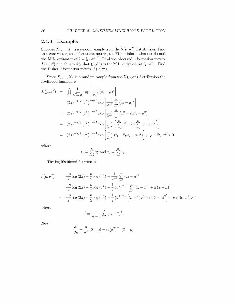
56 CHAPTER 2. MAXIMUM LIKELIHOOD ESTIMATION
2.4.6 Example:
SupposeX1, ...,Xn is a random sample from the N(μ,σ2) distribution. Find
the score vector, the information matrix, the Fisher information matrix and
the M.L. estimator of θ =¡μ,σ2
¢T. Find the observed information matrix
I¡μ, σ2
¢and thus verify that
¡μ, σ2
¢is the M.L. estimator of
¡μ,σ2
¢. Find
the Fisher information matrix J¡μ,σ2
¢.
Since X1, ...,Xn is a random sample from the N¡μ,σ2
¢distribution the
likelihood function is
L¡μ,σ2
¢=
nQi=1
1√2πσ
exp
∙−12σ2
(xi − μ)2¸
= (2π)−n/2¡σ2¢−n/2
exp
∙−12σ2
nPi=1(xi − μ)2
¸= (2π)−n/2
¡σ2¢−n/2
exp
∙−12σ2
nPi=1
¡x2i − 2μxi − μ2
¢¸= (2π)−n/2
¡σ2¢−n/2
exp
∙−12σ2
µnPi=1x2i − 2μ
nPi=1xi + nμ
2
¶¸= (2π)
−n/2 ¡σ2¢−n/2
exp
∙−12σ2
¡t1 − 2μt2 + nμ2
¢¸, μ ∈ <, σ2 > 0
where
t1 =nPi=1x2i and t2 =
nPi=1xi.
The log likelihood function is
l¡μ,σ2
¢=−n2log (2π)− n
2log¡σ2¢− 1
2σ2
nPi=1(xi − μ)
2
=−n2log (2π)− n
2log¡σ2¢− 12
¡σ2¢−1 ∙ nP
i=1(xi − x)2 + n (x− μ)
2
¸=−n2log (2π)− n
2log¡σ2¢− 12
¡σ2¢−1 h
(n− 1) s2 + n (x− μ)2i, μ ∈ <, σ2 > 0
where
s2 =1
n− 1nPi=1
(xi − x)2 .
Now∂l
∂μ=n
σ2(x− μ) = n
¡σ2¢−1
(x− μ)
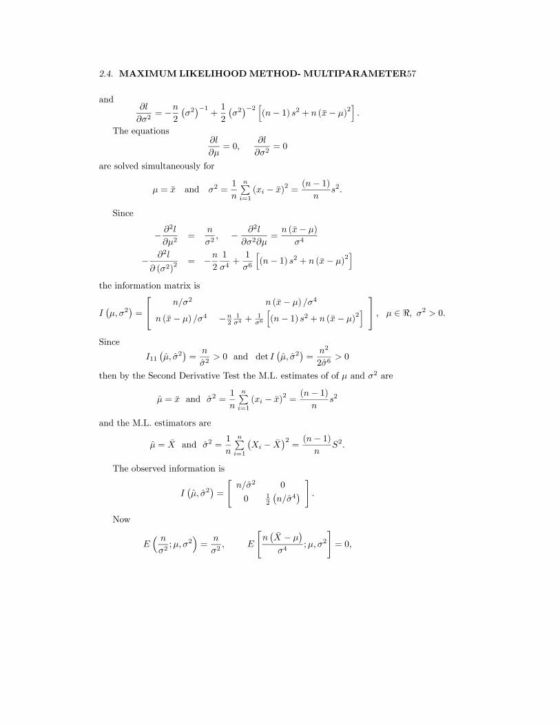
2.4. MAXIMUMLIKELIHOODMETHOD-MULTIPARAMETER57
and∂l
∂σ2= −n
2
¡σ2¢−1
+1
2
¡σ2¢−2 h
(n− 1) s2 + n (x− μ)2i.
The equations∂l
∂μ= 0,
∂l
∂σ2= 0
are solved simultaneously for
μ = x and σ2 =1
n
nPi=1(xi − x)2 =
(n− 1)n
s2.
Since
− ∂2l
∂μ2=
n
σ2, − ∂2l
∂σ2∂μ=n (x− μ)
σ4
− ∂2l
∂ (σ2)2 = −n
2
1
σ4+1
σ6
h(n− 1) s2 + n (x− μ)
2i
the information matrix is
I¡μ,σ2
¢=
⎡⎣ n/σ2 n (x− μ) /σ4
n (x− μ) /σ4 −n21σ4 +
1σ6
h(n− 1) s2 + n (x− μ)2
i ⎤⎦ , μ ∈ <, σ2 > 0.
Since
I11¡μ, σ2
¢=n
σ2> 0 and det I
¡μ, σ2
¢=n2
2σ6> 0
then by the Second Derivative Test the M.L. estimates of of μ and σ2 are
μ = x and σ2 =1
n
nPi=1(xi − x)2 =
(n− 1)n
s2
and the M.L. estimators are
μ = X and σ2 =1
n
nPi=1
¡Xi − X
¢2=(n− 1)n
S2.
The observed information is
I¡μ, σ2
¢=
"n/σ2 0
0 12
¡n/σ4
¢ # .Now
E³ nσ2;μ,σ2
´=n
σ2, E
"n¡X − μ
¢σ4
;μ,σ2
#= 0,
58 CHAPTER 2. MAXIMUM LIKELIHOOD ESTIMATION
and
E
½−n2
1
σ4+1
σ6
h(n− 1)S2 + n
¡X − μ
¢2i;μ,σ2
¾= −n
2
1
σ4+1
σ6
n(n− 1)E(S2;μ,σ2) + nE
h¡X − μ
¢2;μ,σ2
io= −n
2
1
σ4+1
σ6£(n− 1)σ2 + σ2
¤=
n
2σ4
since
E£¡X − μ
¢;μ,σ2
¤= 0,
Eh¡X − μ
¢2;μ,σ2
i= V ar
¡X;μ,σ2
¢=
σ2
nand E
¡S2;μ,σ2
¢= σ2.
Therefore the Fisher information matrix is
J¡μ,σ2
¢=
"nσ2 0
0 n2σ4
#
and the inverse of the Fisher information matrix is
£J¡μ,σ2
¢¤−1=
⎡⎣ σ2
n 0
0 2σ4
n
⎤⎦ .Now
V ar¡X¢=
σ2
n
V ar¡σ2¢= V ar
∙1
n
nPi=1
¡Xi − X
¢2¸=2(n− 1)σ4
n2≈2σ4
n
and
Cov(X, σ2) =1
nCov(X,
nPi=1
¡Xi − X
¢2) = 0
since X andnPi=1
¡Xi − X
¢2are independent random variables. Inferences
for μ and σ2 are usually made using
X − μ
S/√nv t (n− 1) and
(n− 1)S2σ2
v χ2 (n− 1) .
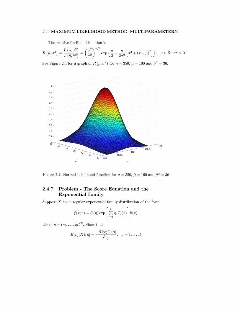
2.4. MAXIMUMLIKELIHOODMETHOD-MULTIPARAMETER59
The relative likelihood function is
R¡μ,σ2
¢=L¡μ,σ2
¢L (μ, σ2)
=
µσ2
σ2
¶n/2exp
nn2− n
2σ2
hσ2 + (x− μ)2
io, μ ∈ <, σ2 > 0.
See Figure 2.4 for a graph of R¡μ,σ2
¢for n = 350, μ = 160 and σ2 = 36.
159159.5
160160.5
161
3032
3436
3840
420
0.1
0.2
0.3
0.4
0.5
0.6
0.7
0.8
0.9
1
μσ2
Figure 2.4: Normal Likelihood function for n = 350, μ = 160 and σ2 = 36
2.4.7 Problem - The Score Equation and theExponential Family
Suppose X has a regular exponential family distribution of the form
f(x; η) = C(η) exp
"kPj=1
ηjTj(x)
#h(x).
where η = (η1, . . . , ηk)T . Show that
E[Tj(X); η] =−∂ logC (η)
∂ηj, j = 1, . . . , k
60 CHAPTER 2. MAXIMUM LIKELIHOOD ESTIMATION
and
Cov(Ti(X), Tj(X); η) =−∂2 logC (η)
∂ηi∂ηj, i, j = 1, . . . , k.
Suppose that (x1, . . . , xn) are the observed data for a random samplefrom fη(x). Show that the score equations
∂
∂ηjl (η) = 0, j = 1, ..., k
can be written as
E
∙nPi=1Tj(Xi); η
¸=
nPi=1Tj(xi), j = 1, . . . , k.
2.4.8 Problem
Suppose X1, . . . ,Xn is a random sample from the N(μ,σ2) distribution.Use the result of Problem 2.4.7 to find the score equations for μ and σ2 andverify that these are the same equations obtained in Example 2.4.7.
2.4.9 Problem
Suppose (X1, Y1) , . . . , (Xn, Yn) is a random sample from the BVN(μ,Σ)distribution. Find the M.L. estimators of μ1, μ2, σ
21 , σ
22, and ρ. You do not
need to verify that your answer corresponds to a maximum. Hint: Use theresult from Problem 2.4.7.
2.4.10 Problem
Suppose (X1,X2) ∼ MULT(n, θ1, θ2). Find the M.L. estimators of θ1 andθ2, the score function and the Fisher information matrix.
2.4.11 Problem
Suppose X1, . . . ,Xn is a random sample from the UNIF(a, b) distribution.Find the M.L. estimators of a and b. Verify that your answer correspondsto a maximum. Find the M.L. estimator of τ(a, b) = E (Xi).
2.4.12 Problem
Suppose X1, . . . ,Xn is a random sample from the UNIF(μ − 3σ,μ + 3σ)distribution. Find the M.L. estimators of μ and σ.
2.4. MAXIMUMLIKELIHOODMETHOD-MULTIPARAMETER61
2.4.13 Problem
Suppose X1, . . . ,Xn is a random sample from the EXP(β,μ) distribution.Find the M.L. estimators of β and μ. Verify that your answer correspondsto a maximum. Find the M.L. estimator of τ(β,μ) = xα where xα is the αpercentile of the distribution.
2.4.14 Problem
In Problem 1.7.26 find the M.L. estimators of μ and σ2. Verify that youranswer corresponds to a maximum.
2.4.15 Problem
Suppose E(Y ) = Xβ where Y = (Y1, . . . , Yn)T is a vector of independent
and normally distributed random variables with V ar(Yi) = σ2, i = 1, . . . , n,X is a n× k matrix of known constants of rank k and β = (β1, . . . ,βk)
T isa vector of unknown parameters. Show that the M.L. estimators of β andσ2 are given by
β =¡XTX
¢−1XTY and σ2 = (Y −Xβ)T (Y −Xβ)/n.
2.4.16 Newton’s Method
In the multiparameter case θ = (θ1, . . . , θk)T Newton’s method is given by:
θ(i+1) = θ(i) + [I(θ(i))]−1S(θ(i)), i = 0, 1, 2, . . .
I(θ) can also be replaced by the Fisher information J(θ).
2.4.17 Example
The following data are 30 independent observations from a BETA(a, b)distribution:
0.2326, 0.0465, 0.2159, 0.2447, 0.0674, 0.3729, 0.3247, 0.3910, 0.3150,0.3049, 0.4195, 0.3473, 0.2709, 0.4302, 0.3232, 0.2354, 0.4014, 0.3720,0.5297, 0.1508, 0.4253, 0.0710, 0.3212, 0.3373, 0.1322, 0.4712, 0.4111,0.1079, 0.0819, 0.3556
The likelihood function for observations x1, x2, ..., xn is
L(a, b) =nQi=1
Γ(a+ b)
Γ(a)Γ(b)xa−1i (1− xi)b−1 , a > 0, b > 0
=
∙Γ(a+ b)
Γ(a)Γ(b)
¸n ∙ nQi=1xi
¸a−1 ∙ nQi=1(1− xi)
¸b−1.
62 CHAPTER 2. MAXIMUM LIKELIHOOD ESTIMATION
The log likelihood function is
l(a, b) = n [logΓ(a+ b)− logΓ(a)− logΓ(b) + (a− 1)t1 + (b− 1)t2]
where
t1 =1
n
nPi=1
log xi and t2 =1
n
nPi=1
log(1− xi).
(T1, T2) is a sufficient statistic for (a, b) where
T1 =1
n
nPi=1logXi and T2 =
1
n
nPi=1log(1−Xi).
Why?Let
Ψ (z) =d logΓ(z)
dz=Γ0 (z)
Γ(z)
which is called the digamma function. The score vector is
S (a, b) =
∙∂l/∂a∂l/∂b
¸= n
"Ψ (a+ b)−Ψ (a) + t1Ψ (a+ b)−Ψ (b) + t2
#.
S (a, b) = [0 0]T must be solved numerically to find the M.L. estimates ofa and b.
Let
Ψ0 (z) =d
dzΨ (z)
which is called the trigamma function. The information matrix is
I(a, b) = n
"Ψ0 (a)−Ψ0 (a+ b) −Ψ0 (a+ b)−Ψ0 (a+ b) Ψ0 (b)−Ψ0 (a+ b)
#
which is also the Fisher or expected information matrix.
For the data above
t1 =1
30
nPi=1log xi = −1.3929 and t2 =
1
30log
nPi=1log(1− xi) = −0.3594.
The M.L. estimates of a and b can be found using Newton’s Method givenby ∙
a(i+1)
b(i+1)
¸=
∙a(i)
b(i)
¸+hI(a(i), b(i))
i−1S(a(i), b(i))
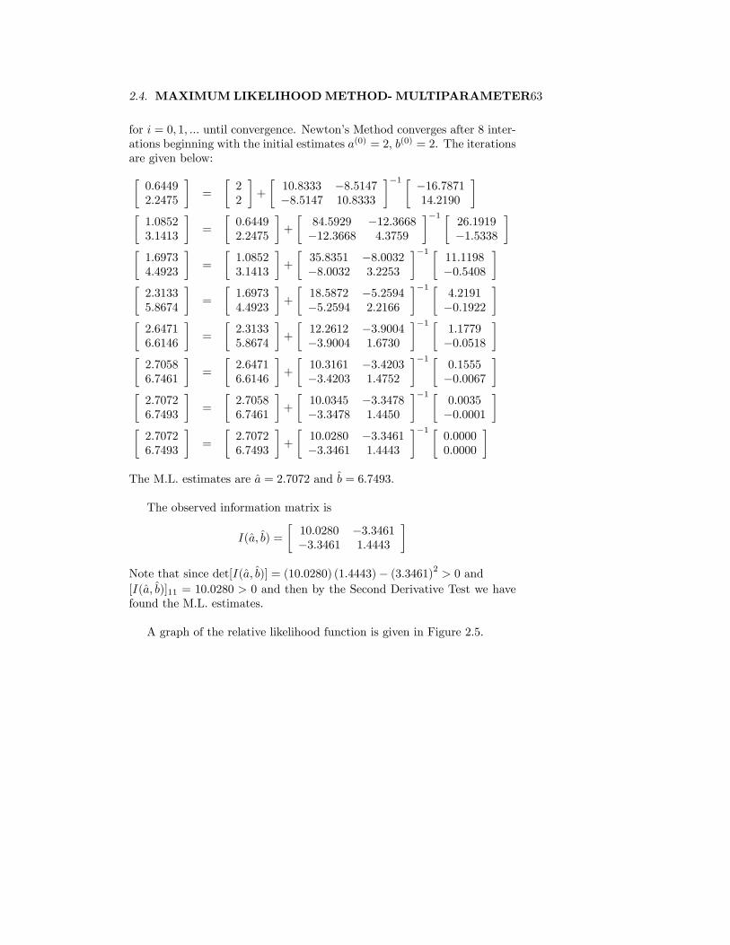
2.4. MAXIMUMLIKELIHOODMETHOD-MULTIPARAMETER63
for i = 0, 1, ... until convergence. Newton’s Method converges after 8 inter-ations beginning with the initial estimates a(0) = 2, b(0) = 2. The iterationsare given below:∙0.64492.2475
¸=
∙22
¸+
∙10.8333 −8.5147−8.5147 10.8333
¸−1 ∙ −16.787114.2190
¸∙1.08523.1413
¸=
∙0.64492.2475
¸+
∙84.5929 −12.3668−12.3668 4.3759
¸−1 ∙26.1919−1.5338
¸∙1.69734.4923
¸=
∙1.08523.1413
¸+
∙35.8351 −8.0032−8.0032 3.2253
¸−1 ∙11.1198−0.5408
¸∙2.31335.8674
¸=
∙1.69734.4923
¸+
∙18.5872 −5.2594−5.2594 2.2166
¸−1 ∙4.2191−0.1922
¸∙2.64716.6146
¸=
∙2.31335.8674
¸+
∙12.2612 −3.9004−3.9004 1.6730
¸−1 ∙1.1779−0.0518
¸∙2.70586.7461
¸=
∙2.64716.6146
¸+
∙10.3161 −3.4203−3.4203 1.4752
¸−1 ∙0.1555−0.0067
¸∙2.70726.7493
¸=
∙2.70586.7461
¸+
∙10.0345 −3.3478−3.3478 1.4450
¸−1 ∙0.0035−0.0001
¸∙2.70726.7493
¸=
∙2.70726.7493
¸+
∙10.0280 −3.3461−3.3461 1.4443
¸−1 ∙0.00000.0000
¸The M.L. estimates are a = 2.7072 and b = 6.7493.
The observed information matrix is
I(a, b) =
∙10.0280 −3.3461−3.3461 1.4443
¸Note that since det[I(a, b)] = (10.0280) (1.4443)− (3.3461)2 > 0 and[I(a, b)]11 = 10.0280 > 0 and then by the Second Derivative Test we havefound the M.L. estimates.
A graph of the relative likelihood function is given in Figure 2.5.
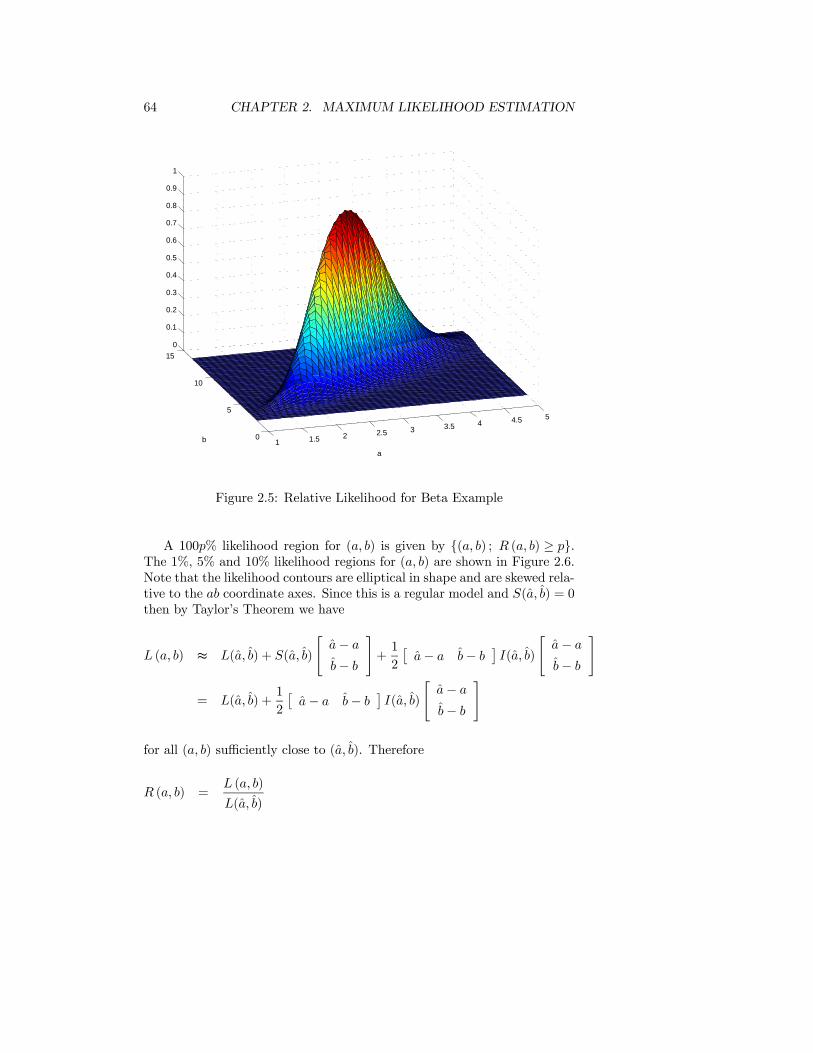
64 CHAPTER 2. MAXIMUM LIKELIHOOD ESTIMATION
1 1.5 2 2.5 3 3.5 4 4.5 5
0
5
10
150
0.1
0.2
0.3
0.4
0.5
0.6
0.7
0.8
0.9
1
a
b
Figure 2.5: Relative Likelihood for Beta Example
A 100p% likelihood region for (a, b) is given by (a, b) ; R (a, b) ≥ p.The 1%, 5% and 10% likelihood regions for (a, b) are shown in Figure 2.6.Note that the likelihood contours are elliptical in shape and are skewed rela-tive to the ab coordinate axes. Since this is a regular model and S(a, b) = 0then by Taylor’s Theorem we have
L (a, b) ≈ L(a, b) + S(a, b)
"a− ab− b
#+1
2
£a− a b− b
¤I(a, b)
"a− ab− b
#
= L(a, b) +1
2
£a− a b− b
¤I(a, b)
"a− ab− b
#
for all (a, b) sufficiently close to (a, b). Therefore
R (a, b) =L (a, b)
L(a, b)
2.4. MAXIMUMLIKELIHOODMETHOD-MULTIPARAMETER65
≈ 1−h2L(a, b)
i−1 £a− a b− b
¤I(a, b)
"a− ab− b
#
= 1−h2L(a, b)
i−1 £a− a b− b
¤ ∙ I11 I12I12 I22
¸"a− ab− b
#
= 1−h2L(a, b)
i−1 h(a− a)2 I11 + 2 (a− a) (b− b)I12 + (b− b)2I22
i.
The set of points (a, b) which satisfy R (a, b) = p is approximately the setof points (a, b) which satisfy
(a− a)2 I11 + 2 (a− a) (b− b)I12 + (b− b)2I22 = 2 (1− p)L(a, b)
which we recognize as the points on an ellipse centred at (a, b). The skew-ness of the likelihood contours relative to the ab coordinate axes is deter-mined by the value of I12. If this value is close to zero the skewness will besmall.
2.4.18 Problem
The following data are 30 independent observations from a GAM(α,β)distribution:
15.1892, 19.3316, 1.6985, 2.0634, 12.5905, 6.0094,13.6279, 14.7847, 13.8251, 19.7445, 13.4370, 18.6259,2.7319, 8.2062, 7.3621, 1.6754, 10.1070, 3.2049,21.2123, 4.1419, 12.2335, 9.8307, 3.6866, 0.7076,7.9571, 3.3640, 12.9622, 12.0592, 24.7272, 12.7624
For these data t1 =30Pi=1log xi = 61.1183 and t2 =
30Pi=1xi = 309.8601.
Find the M.L. estimates of α and β for these data, the observed informationI(α, β) and the Fisher information J(α,β). On the same graph plot the1%, 5%, and 10% likelihood regions for (α,β). Comment.
2.4.19 Problem
Suppose X1, . . . ,Xn is a random sample from the distribution with proba-bility density function
f (x;α,β) =αβ
(1 + βx)α+1x > 0; α,β > 0.
Find the Fisher information matrix J(α,β).
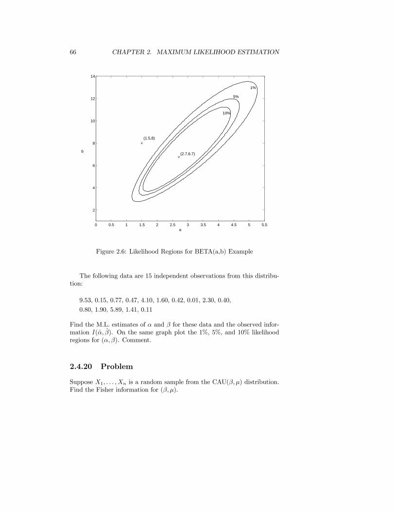
66 CHAPTER 2. MAXIMUM LIKELIHOOD ESTIMATION
a
b
10%
5%
1%
(1.5,8)
(2.7,6.7)
0 0.5 1 1.5 2 2.5 3 3.5 4 4.5 5 5.5
2
4
6
8
10
12
14
Figure 2.6: Likelihood Regions for BETA(a,b) Example
The following data are 15 independent observations from this distribu-tion:
9.53, 0.15, 0.77, 0.47, 4.10, 1.60, 0.42, 0.01, 2.30, 0.40,
0.80, 1.90, 5.89, 1.41, 0.11
Find the M.L. estimates of α and β for these data and the observed infor-mation I(α, β). On the same graph plot the 1%, 5%, and 10% likelihoodregions for (α,β). Comment.
2.4.20 Problem
Suppose X1, . . . ,Xn is a random sample from the CAU(β,μ) distribution.Find the Fisher information for (β,μ).
2.5. INCOMPLETE DATA AND THE E.M. ALGORITHM 67
2.4.21 Problem
A radioactive sample emits particles at a rate which decays with time,the rate being λ(t) = λe−βt. In other words, the number of particlesemitted in an interval (t, t+ h) has a Poisson distribution with parametert+hRt
λe−βsds and the number emitted in disjoint intervals are independent
random variables. Find the M.L. estimate of λ and β, λ > 0, β > 0 ifthe actual times of the first, second, ..., n’th decay t1 < t2 < . . . tn areobserved. Show that β satisfies the equation
βtn
eβtn − 1= 1− βt where t =
1
n
nPi=1ti.
2.4.22 Problem
In Problem 2.1.23 suppose θ = (θ1, . . . , θk)T . Find the Fisher information
matrix and explain how you would find the M.L. estimate of θ.
2.5 Incomplete Data and The E.M. Algorithm
The E.M. algorithm, which was popularized by Dempster, Laird and Rubin(1977), is a useful method for finding M.L. estimates when some of thedata are incomplete but can also be applied to many other contexts suchas grouped data, mixtures of distributions, variance components and factoranalysis.The following are two examples of incomplete data:
2.5.1 Censored Exponential Data
Suppose Xi ∼ EXP(θ), i = 1, . . . , n. Suppose we only observe Xi for mobservations and the remaining n−m observations are censored at a fixedtime c. The observed data are of the form Yi = min(Xi, c), i = 1, . . . , n.Note that Y = Y (X) is a many-to-one mapping. (X1, . . . ,Xn) are calledthe complete data and (Y1, . . . , Yn) are called the incomplete data.
2.5.2 “Lumped” Hardy-Weinberg Data
A gene has two forms A and B. Each individual has a pair of these genes,one from each parent, so that there are three possible genotypes: AA, ABand BB. Suppose that, in both male and female populations, the proportionof A types is equal to θ and the proportion of B types is equal to 1 − θ.
68 CHAPTER 2. MAXIMUM LIKELIHOOD ESTIMATION
Suppose further that random mating occurs with respect to this gene pair.Then the proportion of individuals with genotypes AA, AB and BB in thenext generation are θ2, 2θ(1− θ) and (1− θ)2 respectively. Furthermore, ifrandom mating continues, these proportions will remain nearly constant forgeneration after generation. This is the famous result from genetics calledthe Hardy-Weinberg Law. Suppose we have a group of n individuals andlet X1 = number with genotype AA, X2 = number with genotype AB andX3 = number with genotype BB. Suppose however that it is not possibleto distinguish AA0s from AB0s so that the observed data are (Y1, Y2) whereY1 = X1 +X2 and Y2 = X3. The complete data are (X1,X2,X3) and theincomplete data are (Y1, Y2).
2.5.3 Theorem
Suppose X, the complete data, has probability (density) function f (x; θ)and Y = Y (X), the incomplete data, has probability (density) functiong(y; θ). Suppose further that f (x; θ) and g (x; θ) are regular models. Then
∂
∂θlog g(y; θ) = E[S(θ;X)|Y = y].
Suppose θ, the value which maximizes log g(y; θ), is found by solving∂∂θ log g(y; θ) = 0. By the previous theorem θ is also the solution to
E[S(θ;X)|Y = y; θ] = 0.
Note that θ appears in two places in the second equation, as an argumentin the function S as well as an argument in the expectation E.
2.5.4 The E.M. Algorithm
The E.M. algorithm solves E[S(θ;X)|Y = y] = 0 using an iterative two-stepmethod. Let θ(i) be the estimate of θ from the ith iteration.
(1) E-Step (Expectation Step)
Calculate
Ehlog f (X; θ) |Y = y; θ(i)
i= Q(θ, θ(i)).
(2) M-step (Maximization Step)
2.5. INCOMPLETE DATA AND THE E.M. ALGORITHM 69
Find the value of θ which maximizes Q(θ, θ(i)) and set θ(i+1) equal tothis value. θ(i+1) is found by solving
∂
∂θQ(θ, θ(i)) = E
∙∂
∂θlog f (X; θ) |Y = y; θ(i)
¸= E
hS(θ;X)|Y = y; θ(i)
i= 0
with respect to θ.Note that
EhS(θ(i+1);X)|Y = y; θ(i)
i= 0
2.5.5 Example
Give the E.M. algorithm for the “Lumped” Hardy-Weinberg example. Findθ if n = 10 and y1 = 3. Show how θ can be found explicitly by solving∂∂θ log g(y; θ) = 0 directly.
The complete data (X1,X2) have joint p.f.
f (x1, x2; θ) =n!
x1!x2! (n− x1 − x2)!£θ2¤x1[2θ (1− θ)]
x2h(1− θ)
2in−x1−x2
= θ2x1+x2 (1− θ)2n−(2x1+x2) · h (x1, x2)x1, x2 = 0, 1, . . . ; x1 + x2 ≤ n; 0 < θ < 1
where
h (x1, x2) =n!
x1!x2! (n− x1 − x2)!2x2 .
It is easy to see (show it!) that (X1,X2) has a regular exponential familydistribution with natural sufficient statistic T = T (X1,X2) = 2X1 + X2.The incomplete data are Y = X1 +X2.
For the E-Step we need to calculate
Q(θ, θ(i)) = Ehlog f (X1,X2; θ) |Y = y; θ(i)
i= E
n(2X1 +X2) log θ + [2n− (2X1 +X2)] log (1− θ) |Y = X1 +X2 = y; θ(i)
o+E
hh (X1,X2) |Y = X1 +X2 = y; θ(i)
i. (2.1)
To find these expectations we note that by the properties of the multino-mial distribution
X1|X1 +X2 = y v BINµy,
θ2
θ2 + 2θ (1− θ)
¶= BIN
µy,
θ
2− θ
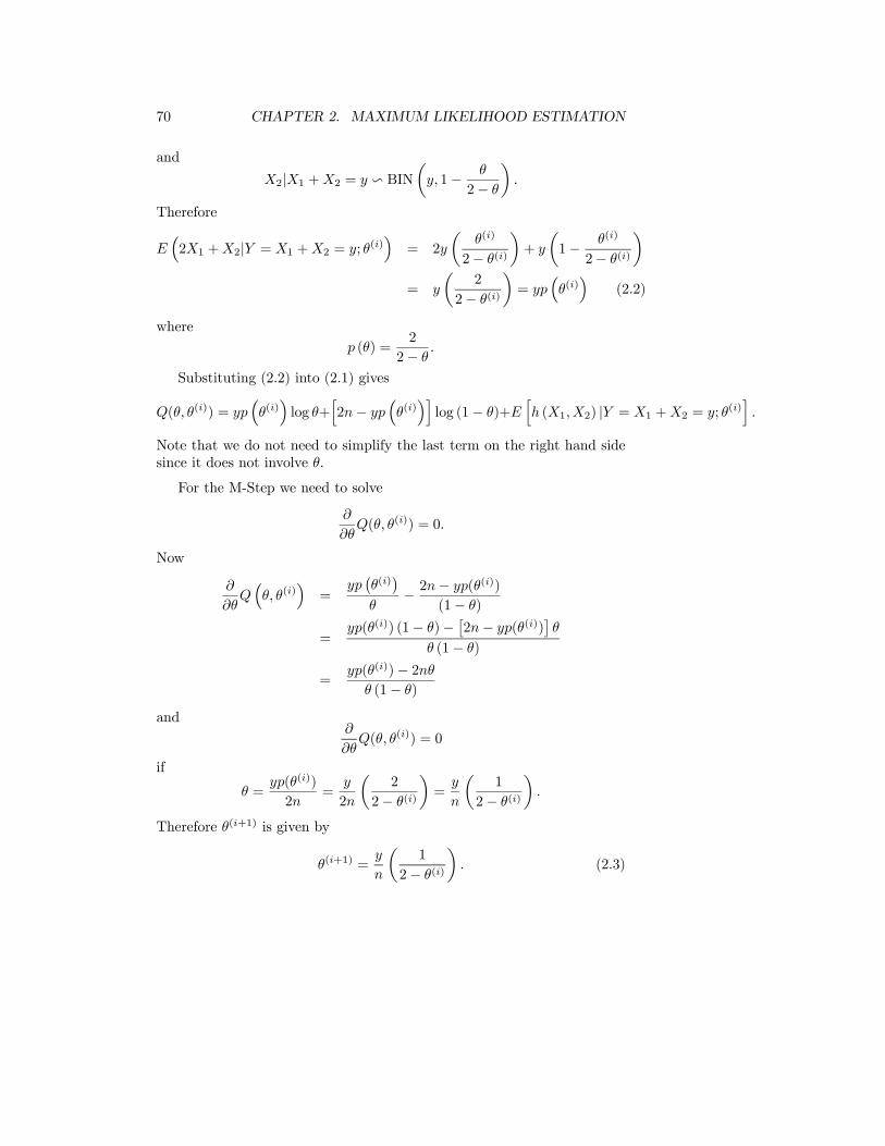
70 CHAPTER 2. MAXIMUM LIKELIHOOD ESTIMATION
and
X2|X1 +X2 = y v BINµy, 1− θ
2− θ
¶.
Therefore
E³2X1 +X2|Y = X1 +X2 = y; θ(i)
´= 2y
µθ(i)
2− θ(i)
¶+ y
µ1− θ(i)
2− θ(i)
¶= y
µ2
2− θ(i)
¶= yp
³θ(i)´
(2.2)
where
p (θ) =2
2− θ.
Substituting (2.2) into (2.1) gives
Q(θ, θ(i)) = yp³θ(i)´log θ+
h2n− yp
³θ(i)´ilog (1− θ)+E
hh (X1,X2) |Y = X1 +X2 = y; θ(i)
i.
Note that we do not need to simplify the last term on the right hand sidesince it does not involve θ.
For the M-Step we need to solve
∂
∂θQ(θ, θ(i)) = 0.
Now
∂
∂θQ³θ, θ(i)
´=
yp¡θ(i)¢
θ− 2n− yp(θ
(i))
(1− θ)
=yp(θ(i)) (1− θ)−
£2n− yp(θ(i))
¤θ
θ (1− θ)
=yp(θ(i))− 2nθ
θ (1− θ)
and∂
∂θQ(θ, θ(i)) = 0
if
θ =yp(θ(i))
2n=y
2n
µ2
2− θ(i)
¶=y
n
µ1
2− θ(i)
¶.
Therefore θ(i+1) is given by
θ(i+1) =y
n
µ1
2− θ(i)
¶. (2.3)
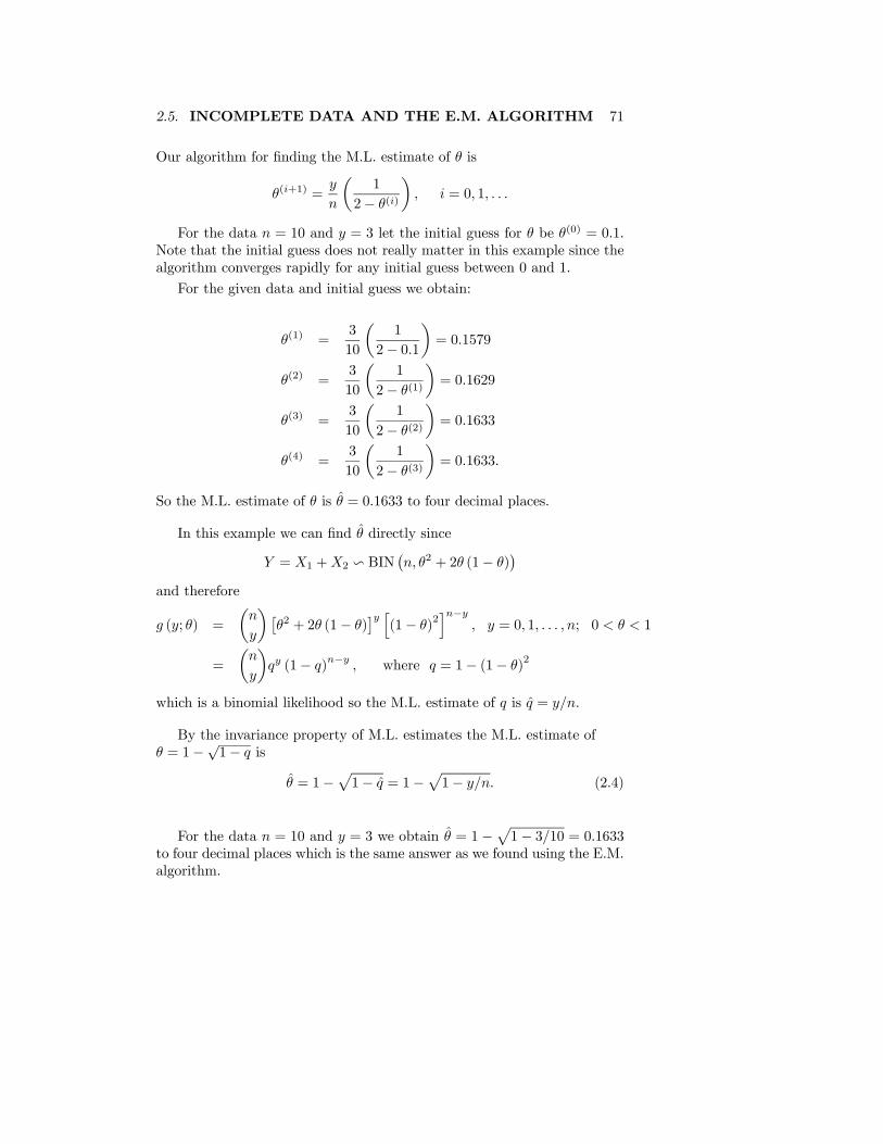
2.5. INCOMPLETE DATA AND THE E.M. ALGORITHM 71
Our algorithm for finding the M.L. estimate of θ is
θ(i+1) =y
n
µ1
2− θ(i)
¶, i = 0, 1, . . .
For the data n = 10 and y = 3 let the initial guess for θ be θ(0) = 0.1.Note that the initial guess does not really matter in this example since thealgorithm converges rapidly for any initial guess between 0 and 1.
For the given data and initial guess we obtain:
θ(1) =3
10
µ1
2− 0.1
¶= 0.1579
θ(2) =3
10
µ1
2− θ(1)
¶= 0.1629
θ(3) =3
10
µ1
2− θ(2)
¶= 0.1633
θ(4) =3
10
µ1
2− θ(3)
¶= 0.1633.
So the M.L. estimate of θ is θ = 0.1633 to four decimal places.
In this example we can find θ directly since
Y = X1 +X2 v BIN¡n, θ2 + 2θ (1− θ)
¢and therefore
g (y; θ) =
µn
y
¶£θ2 + 2θ (1− θ)
¤y h(1− θ)
2in−y
, y = 0, 1, . . . , n; 0 < θ < 1
=
µn
y
¶qy (1− q)n−y , where q = 1− (1− θ)
2
which is a binomial likelihood so the M.L. estimate of q is q = y/n.
By the invariance property of M.L. estimates the M.L. estimate ofθ = 1−
√1− q is
θ = 1−p1− q = 1−
p1− y/n. (2.4)
For the data n = 10 and y = 3 we obtain θ = 1−p1− 3/10 = 0.1633
to four decimal places which is the same answer as we found using the E.M.algorithm.
72 CHAPTER 2. MAXIMUM LIKELIHOOD ESTIMATION
2.5.6 E.M. Algorithm and the Regular ExponentialFamily
SupposeX, the complete data, has a regular exponential family distributionwith probability (density) function
f(x; θ) = C(θ) exp
"kPj=1
qj (θ)Tj(x)
#h(x), θ = (θ1, . . . , θk)
T
and let Y = Y (X) be the incomplete data. Then the M-step of the E.M.algorithm is given by
E[Tj(X); θ(i+1)] = E[Tj(X)|Y = y; θ(i)], j = 1, . . . , k. (2.5)
2.5.7 Problem
Prove (2.5) using the result from Problem 2.4.7.
2.5.8 Example
Use (2.5) to find the M-step for the “Lumped” Hardy-Weinberg example.
Since the natural sufficient statistic is T = T (X1,X2) = 2X1 +X2 theM-Step is given by
Eh2X1 +X2; θ
(i+1)i= E
h2X1 +X2|Y = y; θ(i)
i. (2.6)
Using (2.2) and the fact that
X1 v BIN¡n, θ2
¢and X2 v BIN (n, 2θ (1− θ)) ,
then (2.6) can be written as
2nhθ(i+1)
i2+ n
h2θ(i+1)
i h1− θ(i+1)
i= y
µ2
2− θ(i)
¶or
θ(i+1) =y
2n
µ2
2− θ(i)
¶=y
n
µ1
2− θ(i)
¶which is the same result as in (2.3).
If the algorithm converges and
limi→∞
θ(i) = θ
2.5. INCOMPLETE DATA AND THE E.M. ALGORITHM 73
(How would you prove this? Hint: Recall the Monotonic Sequence Theo-rem.) then
limi→∞
θ(i+1) = limi→∞
y
n
µ1
2− θ(i)
¶or
θ =y
n
µ1
2− θ
¶.
Solving for θ givesθ = 1−
p1− y/n
which is the same result as in (2.4).
2.5.9 Example
Use (2.5) to give the M-step for the censored exponential data example.
Assuming the algorithm converges, find an expression for θ. Show that thisis the same θ which is obtained when ∂
∂θ log g(y; θ) = 0 is solved directly.
2.5.10 Problem
Suppose X1, . . . ,Xn is a random sample from the N(μ,σ2) distribution.Suppose we observe Xi, i = 1, . . . ,m but for i = m + 1, . . . , n we observeonly that Xi > c.
(a) Give explicitly the M-step of the E.M. algorithm for finding the M.L.estimate of μ in the case where σ2 is known.
(b) Give explicitly the M-step of the E.M. algorithm for finding the M.L.estimates of μ and σ2.
Hint: If Z ∼ N(0, 1) show that
E(Z|Z > b) = φ(b)
1−Φ(b) = h(b)
where φ is the probability density function and Φ is the cumulative distri-bution function of Z and h is called the hazard function.
2.5.11 Problem
Let (X1, Y1) , . . . , (Xn, Yn) be a random sample from the BVN(μ,Σ) dis-tribution. Suppose that some of the Xi and Yi are missing as follows: fori = 1, . . . , n1 we observe both Xi and Yi, for i = n1 + 1, . . . , n2 we observeonly Xi and for i = n2 + 1, . . . , n we observe only Yi. Give explicitly theM-step of the E.M. algorithm for finding the M.L. estimates of
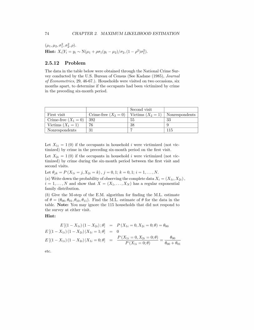
74 CHAPTER 2. MAXIMUM LIKELIHOOD ESTIMATION
(μ1,μ2,σ21 ,σ
22 , ρ).
Hint: Xi|Yi = yi ∼ N(μ1 + ρσ1(yi − μ2)/σ2, (1− ρ2)σ21).
2.5.12 Problem
The data in the table below were obtained through the National Crime Sur-vey conducted by the U.S. Bureau of Census (See Kadane (1985), Journalof Econometrics, 29, 46-67.). Households were visited on two occasions, sixmonths apart, to determine if the occupants had been victimized by crimein the preceding six-month period.
Second visitFirst visit Crime-free (X2 = 0) Victims (X2 = 1) NonrespondentsCrime-free (X1 = 0) 392 55 33Victims (X1 = 1) 76 38 9Nonrespondents 31 7 115
Let X1i = 1 (0) if the occupants in household i were victimized (not vic-timized) by crime in the preceding six-month period on the first visit.
Let X2i = 1 (0) if the occupants in household i were victimized (not vic-timized) by crime during the six-month period between the first visit andsecond visits.
Let θjk = P (X1i = j,X2i = k) , j = 0, 1; k = 0, 1; i = 1, . . . ,N.
(a) Write down the probability of observing the complete dataXi = (X1i,X2i) ,i = 1, . . . , N and show that X = (X1, . . . ,XN) has a regular exponentialfamily distribution.
(b) Give the M-step of the E.M. algorithm for finding the M.L. estimateof θ = (θ00, θ01, θ10, θ11). Find the M.L. estimate of θ for the data in thetable. Note: You may ignore the 115 households that did not respond tothe survey at either visit.
Hint:
E [(1−X1i) (1−X2i) ; θ] = P (X1i = 0,X2i = 0; θ) = θ00
E [(1−X1i) (1−X2i) |X1i = 1; θ] = 0
E [(1−X1i) (1−X2i) |X1i = 0; θ] =P (X1i = 0,X2i = 0; θ)
P (X1i = 0; θ)=
θ00θ00 + θ01
etc.
2.6. THE INFORMATION INEQUALITY 75
(c) Find the M.L. estimate of the odds ratio
τ =θ00θ11θ01θ10
.
What is the significance of τ = 1?
2.6 The Information Inequality
Suppose we consider estimating a parameter τ(θ),where θ is a scalar, usingan unbiased estimator T (X). Is there any limit to how well an estimator likethis can behave? The answer for unbiased estimators is in the affirmative,and a lower bound on the variance is given by the information inequality.
2.6.1 Information Inequality - One Parameter
Suppose T (X) is an unbiased estimator of the parameter τ(θ) in a regularstatistical model f (x; θ) ; θ ∈ Ω. Then
V ar(T ) ≥ [τ0 (θ)]2
J (θ).
Equality holds if and only ifX has a regular exponential family with naturalsufficient statistic T (X).
2.6.2 Proof
Since T is an unbiased estimator of τ(θ),ZA
T (x)f (x; θ) dx = τ(θ), for all θ ∈ Ω,
where P (X ∈ A; θ) = 1. Since f (x; θ) is a regular model we can take thederivative with respect to θ on both sides and interchange the integral andderivative to obtain: Z
A
T (x)∂f (x; θ)
∂θdx = τ 0(θ).
Since E[S(θ;X)] = 0, this can be written as
Cov[T, S(θ;X)] = τ 0(θ)
76 CHAPTER 2. MAXIMUM LIKELIHOOD ESTIMATION
and by the covariance inequality, this implies
V ar(T )V ar[S(θ;X)] ≥ [τ 0(θ]2 (2.7)
which, upon dividing by J(θ) = V ar[S(θ;X)], provides the desired result.Now suppose we have equality in (2.7). Equality in the covariance in-
equality obtains if and only if the random variables T and S(θ;X) are linearfunctions of one another. Therefore, for some (non-random) c1(θ), c2(θ), ifequality is achieved,
S(θ;x) = c1(θ)T (x) + c2(θ) all x ∈ A.
Integrating with respect to θ,
log f (x; θ) = C1(θ)T (x) + C2(θ) + C3(x)
where we note that the constant of integration C3 is constant with respectto changing θ but may depend on x. Therefore,
f (x; θ) = C(θ) exp [C1(θ)T (x)]h(x)
where C(θ) = eC2(θ) and h(x) = eC3(x) which is exponential family withnatural sufficient statistic T (X).¥
The special case of the information inequality that is of most interest isthe unbiased estimation of the parameter θ. The above inequality indicatesthat any unbiased estimator T of θ has variance at least 1/J(θ). The lowerbound is achieved only when f (x; θ) is regular exponential family withnatural sufficient statistic T .
Notes:1. If equality holds then T (X) is called an efficient estimator of τ(θ).2. The number
[τ 0(θ)]2
J(θ)
is called the Cramer-Rao lower bound (C.R.L.B.).3. The ratio of the C.R.L.B. to the variance of an unbiased estimator iscalled the efficiency of the estimator.
2.6.3 Example
Suppose X1, . . . ,Xn is a random sample from the POI(θ) distribution.Show that the variance of the U.M.V.U.E. of θ achieves the Cramer-Rao
2.6. THE INFORMATION INEQUALITY 77
lower bound for unbiased estimators of θ and find the lower bound. Whatis the U.M.V.U.E. of τ(θ) = θ2? Does the variance of this estimator achievethe Cramer-Rao lower bound for unbiased estimators of θ2? What is thelower bound?
2.6.4 Example
Suppose X1, . . . ,Xn is a random sample from the distribution with proba-bility density function
f (x; θ) = θxθ−1, 0 < x < 1, θ > 0.
Show that the variance of the U.M.V.U.E. of θ does not achieve the Cramer-Rao lower bound. What is the efficiency of the U.M.V.U.E.?
For some time it was believed that no estimator of θ could havevariance smaller than 1/J(θ) at any value of θ but this was demonstratedincorrect by the following example of Hodges.
2.6.5 Problem
Let X1, . . . ,Xn is a random sample from the N(θ, 1) distribution and define
T (X) =X
2if |X| ≤ n−1/4, T (X) = X otherwise.
Show that E(T ) ≈ θ, V ar(T ) ≈ 1/n if θ 6= 0, and V ar(T ) ≈ 14n if θ = 0.
Show that the Cramer-Rao lower bound for estimating θ is equal to 1n .
This example indicates that it is possible to achieve variance smallerthan 1/J(θ) at one or more values of θ. It has been proved that this is theexception. In fact the set of θ for which the variance of an estimator is lessthan 1/J(θ) has measure 0, which means, for example, that it may be afinite set or perhaps a countable set, but it cannot contain a non-degenerateinterval of values of θ.
2.6.6 Problem
For each of the following determine whether the variance of the U.M.V.U.E.of θ based on a random sample X1, . . . ,Xn achieves the Cramer-Rao lowerbound. In each case determine the Cramer-Rao lower bound and find theefficiency of the U.M.V.U.E.(a) N(θ, 4)(b) Bernoulli(θ)(c) N(0, θ2)(d) N(0, θ).
78 CHAPTER 2. MAXIMUM LIKELIHOOD ESTIMATION
2.6.7 Problem
Find examples of the following phenomena in a regular statistical model.(a) No unbiased estimator of τ(θ) exists.(b) An unbiased estimator of τ(θ) exists but there is no U.M.V.U.E.(c) A U.M.V.U.E. of τ(θ) exists but its variance is strictly greater than theCramer-Rao lower bound.(d) A U.M.V.U.E. of τ(θ) exists and its variance equals the Cramer-Raolower bound.
2.6.8 Information Inequality - Multiparameter
The right hand side in the information inequality generalizes naturally tothe multiple parameter case in which θ is a vector. For example ifθ = (θ1, . . . , θk)
T , then the Fisher information J(θ) is a k × k matrix. Ifτ(θ) is any real-valued function of θ then its derivative is a column vector
we will denote by D(θ) =³∂τ∂θ1, . . . , ∂τ
∂θk
´T. Then if T (X) is any unbiased
estimator of τ(θ) in a regular model,
V ar(T ) ≥ [D(θ)]T [J(θ)]−1D(θ) for all θ ∈ Ω.
2.6.9 Example
Let X1, . . . ,Xn be a random sample from the N(μ,σ2) distribution. Findthe U.M.V.U.E. of σ and determine whether the U.M.V.U.E. is an efficientestimator of σ. What happens as n→∞? Hint:
Γ (k + a)
Γ (k + b)= ka−b
∙1 +
(a+ b− 1) (a− b)2k
+O
µ1
k2
¶¸as k →∞
2.6.10 Problem
Let X1, . . . ,Xn be a random sample from the N(μ,σ2) distribution. Findthe U.M.V.U.E. of μ/σ and determine whether the U.M.V.U.E. is an effi-cient estimator. What happens as n→∞?
2.6.11 Problem
Let X1, . . . ,Xn be a random sample from the GAM(α,β) distribution.Find the U.M.V.U.E. of E(Xi;α,β) = αβ and determine whether theU.M.V.U.E. is an efficient estimator.
2.7. ASYMPTOTIC PROPERTIES OFM.L.ESTIMATORS - ONE PARAMETER 79
2.6.12 Problem
Consider the model in Problem 1.7.26.
(a) Find the M.L. estimators of μ and σ2 using the result from Problem2.4.7. You do not need to verify that your answer corresponds to a maxi-mum. Compare the M.L. estimators with the U.M.V.U.E.’s of μ and σ2.
(b) Find the observed information matrix and the Fisher information.
(c) Determine if the U.M.V.U.E.’s of μ and σ2 are efficient estimators.
2.7 Asymptotic Properties of M.L.Estimators - One Parameter
One of the more successful attempts at justifying estimators and demon-strating some form of optimality has been through large sample theory orthe asymptotic behaviour of estimators as the sample size n → ∞. Oneof the first properties one requires is consistency of an estimator. Thismeans that the estimator converges to the true value of the parameter asthe sample size (and hence the information) approaches infinity.
2.7.1 Definition
Consider a sequence of estimators Tn where the subscript n indicates thatthe estimator has been obtained from data X1, . . . ,Xn with sample size n.Then the sequence is said to be a consistent sequence of estimators of τ(θ)if Tn →p τ(θ) for all θ ∈ Ω.
It is worth a reminder at this point that probability (density) functionsare used to produce probabilities and are only unique up to a point. Forexample if two probability density functions f(x) and g(x) were such thatthey produced the same probabilities, or the same cumulative distributionfunction, for example,
xZ−∞
f(z)dz =
xZ−∞
g(z)dz
for all x, then we would not consider them distinct probability densities,even though f(x) and g(x) may differ at one or more values of x. Nowwhen we parameterize a given statistical model using θ as the parameter, itis natural to do so in such a way that different values of the parameter leadto distinct probability (density) functions. This means, for example, that
80 CHAPTER 2. MAXIMUM LIKELIHOOD ESTIMATION
the cumulative distribution functions associated with these densities aredistinct. Without this assumption it would be impossible to accurately es-timate the parameter since two different parameters could lead to the samecumulative distribution function and hence exactly the same behaviour ofthe observations. Therefore we assume:
(R7) The probability (density) functions corresponding to different valuesof the parameters are distinct, that is, θ 6= θ∗ =⇒ f (x; θ) 6= f (x; θ∗).This assumption together with assumptions (R1)− (R6) (see 2.3.1) are
sufficient conditions for the theorems given in this section.
2.7.2 Theorem - Consistency of the M.L. Estimator(Regular Model)
Suppose X1, . . . ,Xn is a random sample from a model f (x; θ) ; θ ∈ Ωsatisfying regularity conditions (R1)−(R7). Then with probability tendingto 1 as n→∞, the likelihood equation or score equation
nXi=1
∂
∂θlogf (Xi; θ) = 0
has a root θn such that θn converges in probability to θ0, the true value ofthe parameter, as n→∞.
The proof of this theorem is given in Section 5.4.9 of the Ap-pendix.
The likelihood equation does not always have a unique root as the fol-lowing problem illustrates.
2.7.3 Problem
Indicate whether or not the likelihood equation based on X1, . . . ,Xn has aunique root in each of the cases below:(a) LOG(1, θ)(b) WEI(1, θ)(c) CAU(1, θ)
The consistency of the M.L. estimator is one indication that it performsreasonably well. However, it provides no reason to prefer it to some otherconsistent estimator. The following result indicates that M.L. estimatorsperform as well as any reasonable estimator can, at least in the limit asn→∞.
2.7. ASYMPTOTIC PROPERTIES OFM.L.ESTIMATORS - ONE PARAMETER 81
2.7.4 Theorem - Asymptotic Distribution ofthe M.L. Estimator (Regular Model)
Suppose (R1)− (R7) hold. Suppose θn is a consistent root of the likelihoodequation as in Theorem 2.7.2. Thenp
J(θ0)(θn − θ0)→D Z ∼ N(0, 1)
where θ0 is the true value of the parameter.
The proof of this theorem is given in Section 5.4.10 of theAppendix.
Note: Since J(θ) is the Fisher expected information based on a randomsample from the model f (x; θ) ; θ ∈ Ω,
J(θ) = E
∙−
nPi=1
∂2
∂θ2logf (Xi; θ) ; θ
¸= nE
∙− ∂2
∂θ2logf (X; θ) ; θ
¸where X has probability (density) function f (x; θ).
This theorem implies that for a regular model and sufficiently large n,θn has an approximately normal distribution with mean θ0 and variance[J(θ0)]
−1. [J(θ0)]
−1is called the asymptotic variance of θn. This theorem
also asserts that θn is asymptotically unbiased and its asymptotic varianceapproaches the Cramer-Rao lower bound for unbiased estimators of θ.
By the Limiting Theorems it also follows that
τ(θn)− τ (θ0)q[τ 0 (θ0)]
2 /J (θ0)→D Z v N(0, 1) .
Compare this result with the Information Inequality.
2.7.5 Definition
Suppose X1, . . . ,Xn is a random sample from a regular statistical modelf (x; θ) ; θ ∈ Ω. Suppose also that Tn = Tn(X1, ...,Xn) is asymptoticallynormal with mean θ and variance σ2T /n. The asymptotic efficiency of Tn isdefined to be ½
σ2T ·E∙−∂
2 log f (X; θ)
∂θ2; θ
¸¾−1where X has probability (density) function f (x; θ).
82 CHAPTER 2. MAXIMUM LIKELIHOOD ESTIMATION
2.7.6 Problem
SupposeX1, . . . ,Xn is a random sample from a distribution with continuousprobability density function f (x; θ) and cumulative distribution functionF (x; θ) where θ is the median of the distribution. Suppose also that f (x; θ)is continuous at x = θ. The sample median Tn = med(X1, . . . ,Xn) is apossible estimator of θ.(a) Find the probability density function of the median if n = 2m + 1 isodd.(b) Prove
√n(Tn − θ)→D T ∼ N
µ0,
1
4[f(0; 0)]2
¶(c) If X1, ...,Xn is a random sample from the N(θ, 1) distribution find theasymptotic efficiency of Tn.(d) If X1, ...,Xn is a random sample from the CAU(1, θ) distribution findthe asymptotic efficiency of Tn.
2.8 Interval Estimators
2.8.1 Definition
Suppose X is a random variable whose distribution depends on θ. Supposethat A(x) and B(x) are functions such that A(x) ≤ B(x) for all x ∈ supportof X and θ ∈ Ω. Let x be the observed data. Then (A(x), B(x)) is aninterval estimate for θ. The interval (A(X), B(X)) is an interval estimatorfor θ.
Likelihood intervals are one type of interval estimator. Confidence in-tervals are another type of interval estimator.
We now consider a general approach for constructing confidence inter-vals based on pivotal quantities.
2.8.2 Definition
Suppose X is a random variable whose distribution depends on θ. Therandom variable Q(X; θ) is called a pivotal quantity if the distribution ofQ does not depend on θ. Q(X; θ) is called an asymptotic pivotal quantity ifthe limiting distribution of Q as n→∞ does not depend on θ.
For example, for a random sample X1, . . . ,Xn from a N(θ,σ2) distrib-
2.8. INTERVAL ESTIMATORS 83
ution where σ2 is known, the statistic
T =
√n¡X − θ
¢σ
is a pivotal quantity whose distribution does not depend on θ. IfX1, . . . ,Xnis a random sample from a distribution, not necessarily normal, havingmean θ and known variance σ2 then the asymptotic distribution of T isN(0, 1) by the C.L.T. and T is an asymptotic pivotal quantity.
2.8.3 Definition
Suppose A(X) and B(X) are statistics. If P [A(X) < θ < B(X)] = p,0 < p < 1 then (a(x), b(x)) is called a 100p% confidence interval (C.I.) forθ.
Pivotal quantities can be used for constructing C.I.’s in the followingway. Since the distribution of Q(X; θ) is known we can write down aprobability statement of the form
P (q1 ≤ Q(X; θ) ≤ q2) = p.
If Q is a monotone function of θ then this statement can be rewritten as
P [A(X) ≤ θ ≤ B(X)] = p
and the interval [a(x), b(x)] is a 100p% C.I..
The following theorem gives the pivotal quantity in the case in which θis either a location parameter or a scale parameter.
2.8.4 Theorem
Let X = (X1, ...,Xn) be a random sample from the model f (x; θ) ; θ ∈ Ωand let θ = θ(X) be the M.L. estimator of the scalar parameter θ based onX.
(1) If θ is a location parameter then Q = Q (X) = θ−θ is a pivotal quantity.(2) If θ is a scale parameter then Q = Q (X) = θ/θ is a pivotal quantity.
2.8.5 Asymptotic Pivotal Quantities and ApproximateConfidence Intervals
In cases in which an exact pivotal quantity cannot be constructed we canuse the limiting distribution of θn to construct approximate C.I.’s. Since
[J(θn)]1/2(θn − θ0)→D Z v N(0, 1)
84 CHAPTER 2. MAXIMUM LIKELIHOOD ESTIMATION
then [J(θn)]1/2(θ−θ0) is an asymptotic pivotal quantity and an approximate
100p% C.I. based on this asymptotic pivotal quantity is given byhθn − a[J(θn)]−1/2, θn + a[J(θn)]−1/2
iwhere θn = θn(x1, ..., xn) is the M.L. estimate of θ, P (−a < Z < a) = pand Z v N(0, 1).
Similarly since
[I(θn;X)]1/2(θn − θ0)→D Z v N(0, 1)
where X = (X1, ...,Xn) then [I(θn;X)]1/2(θn−θ0) is an asymptotic pivotal
quantity and an approximate 100p% C.I. based on this asymptotic pivotalquantity is given byh
θn − a[I(θ)]−1/2, θn + a[I(θn)]−1/2i
where I(θn) is the observed information.
Finally since
−2 logR(θ0;X)→D W v χ2(1)
then −2 logR(θ0;X) is an asymptotic pivotal quantity and an approximate100p% C.I. based on this asymptotic pivotal is
θ : −2 logR(θ;x) ≤ b
where x = (x1, ..., xn) are the observed data, P (W ≤ b) = p andW v χ2(1). Usually this must be calculated numerically.
Since
τ(θn)− τ (θ0)rhτ 0(θn)
i2/J(θn)
→D Z v N(0, 1)
an approximate 100p% C.I. for τ (θ) is given by"τ(θn)− a
½hτ 0(θn)
i2/J(θn)
¾1/2, τ(θn) + a
½hτ 0(θn)
i2/J(θn)
¾1/2#
where P (−a < Z < a) = p and Z v N(0, 1).
2.8. INTERVAL ESTIMATORS 85
2.8.6 Likelihood Intervals and Approximate ConfidenceIntervals
A 15% L.I. for θ is given by θ : R(θ;x) ≥ 0.15. Since
−2 logR(θ0;X)→D W v χ2(1)
we have
P [R(θ;X) ≥ 0.15] = P [−2 logR(θ;X) ≤ −2 log (0.15)]= P [−2 logR(θ;X) ≤ 3.79]≈ P (W ≤ 3.79) = P
¡Z2 ≤ 3.79
¢where Z v N(0, 1)
≈ P (−1.95 ≤ Z ≤ 1.95)≈ 0.95
and therefore a 15% L.I. is an approximate 95% C.I. for θ.
2.8.7 Example
Suppose X1, . . . ,Xn is a random sample from the distribution with proba-bility density function
f (x; θ) = θxθ−1, 0 < x < 1.
The likelihood function for observations x1, . . . , xn is
L (θ) =nQi=1
θxθ−1i = θnµ
nQi=1xi
¶θ−1, θ > 0
The log likelihood and score function are
l (θ) = n log θ + (θ − 1)nPi=1log xi, θ > 0
S (θ) =n
θ+ t =
1
θ(n+ tθ)
where t =nPi=1log xi. Since
S (θ) > 0 for 0 < θ < −n/t and S (θ) < 0 for θ > −n/t
therefore by the First Derivative Test, θ = −n/t is the M.L. estimate of θ.The M.L. estimator of θ is θ = −n/T where T =
nPi=1logXi.
86 CHAPTER 2. MAXIMUM LIKELIHOOD ESTIMATION
The information function is
I (θ) =n
θ2, θ > 0
and the Fisher information is
J (θ) = E [I (θ;X)] = E³ nθ2
´=n
θ2
By the W.L.L.N.
−Tn= − 1
n
nPi=1logXi →p E (− logXi; θ0) =
1
θ0
and by the Limit Theorems
θn =n
T→p θ0
and thus θn is a consistent estimator of θ0.
By Theorem 2.7.4pJ (θ0)(θn − θ0) =
rn
θ20(θn − θ0)→D Z v N(0, 1) . (2.8)
The asymptotic variance of θn is equal to θ20/n whereas the actual variance
of θn is
V ar(θn) =n2θ20
(n− 1)2 (n− 2).
This can be shown using the fact that − logXi v EXP(1/θ0), i = 1, . . . , nindependently which means
T = −nPi=1logXi v GAM
µn,1
θ0
¶(2.9)
and then using the result from Problem 1.3.4. Therefore the asymptoticvariance and the actual variance of θn are not identical but are close invalue for large n.
An approximate 95% C.I. for θ based onqJ(θn)(θn − θ0)→D Z v N(0, 1)
is given by∙θn − 1.96/
qJ(θn), θn + 1.96/
qJ(θn)
¸=hθn − 1.96θn/
√n, θn + 1.96θn/
√ni.
2.8. INTERVAL ESTIMATORS 87
Note the width of the C.I. which is equal to 2 (1.96) θn/√n decreases as
1/√n.
An exact C.I. for θ can be obtained in this case since
T
θ−1= Tθ =
nθ
θv GAM(n, 1)
and therefore nθ/θ is a pivotal quantitiy. Since
2Tθ =2nθ
θv χ2 (2n)
we can use values from the chi-squared tables. From the chi-squared tableswe find values a and b such that
P (a ≤W ≤ b) = 0.95 where W v χ2 (2n) .
Then
P
µa ≤ 2nθ
θ≤ b¶= 0.95
or
P
Ãaθ
2n≤ θ ≤ bθ
2n
!= 0.95
and a 95% C.I. for θ is "aθ
2n,bθ
2n
#.
If we choose
P (W ≤ a) = 1− 0.952
= 0.025 = P (W ≥ b)
then we obtain an “equal-tail” C.I. for θ. This is not the narrowest C.I.but it is easier to obtain than the narrowest C.I.. How would you obtainthe narrowest C.I.?
2.8.8 Example
Suppose X1, . . . ,Xn is a random sample from the POI (θ) distribution. Theparameter θ is neither a location or scale parameter. The M.L. estimatorof θ and the Fisher information are
θn = Xn and J (θ) =n
θ.
88 CHAPTER 2. MAXIMUM LIKELIHOOD ESTIMATION
By Theorem 2.7.4
pJ (θ0)
³θn − θ0
´=
rn
θ0
³θn − θ0
´→D Z v N(0, 1) . (2.10)
By the C.L.T.Xn − θ0p
θ0/n→D Z v N(0, 1)
which is the same result.
The asymptotic variance of θn is equal to θ0/n. Since the actual variance
of θn is
V ar(θn) = V ar¡Xn¢=
θ0n
the asymptotic variance and the actual variance of θn are identical in thiscase.
An approximate 95% C.I. for θ based onqJ(θn)
³θn − θ0
´→D Z v N(0, 1)
is given by∙θn − 1.96/
qJ(θn), θn + 1.96/
qJ(θn)
¸=
∙θn − 1.96
qθn/n, θn + 1.96
qθn/n
¸.
An approximate 95% C.I. for τ (θ) = e−θ can be based on the asymptoticpivotal
τ(θn)− τ (θ0)rhτ 0(θn)
i2/J(θn)
→D Z v N(0, 1) .
For τ (θ) = e−θ = P (X1 = 0; θ), τ0 (θ) = d
dθ
¡e−θ
¢= −e−θ and the approx-
imate 95% C.I. is given by"τ³θn
´− 1.96
½hτ 0(θn)
i2/J(θn)
¾1/2, τ³θn
´− 1.96
½hτ 0(θn)
i2/J(θn)
¾1/2#
=
∙e−θn − 1.96e−θn
qθn/n, e
−θn + 1.96e−θnqθn/n
¸. (2.11)
which is symmetric about the M.L. estimate τ(θn) = e−θn .
2.8. INTERVAL ESTIMATORS 89
Alternatively since
0.95 ≈ P
µθn − 1.96
qθn/n ≤ θ ≤ θn + 1.96
qθn/n
¶= P
µ−θn + 1.96
qθn/n ≥ −θ ≥ −θn − 1.96
qθn/n
¶= P
µexp
µ−θn + 1.96
qθn/n
¶≥ e−θ ≥ exp
µ−θn − 1.96
qθn/n
¶¶= P
µexp
µ−θn − 1.96
qθn/n
¶≤ e−θ ≤ exp
µ−θn + 1.96
qθn/n
¶¶therefore∙
exp
µ−θn − 1.96
qθn/n
¶, exp
µ−θn + 1.96
qθn/n
¶¸(2.12)
is also an approximate 95% C.I. for τ (θ).
If n = 20 and θn = 3 then the C.I. (2.11) is equal to [0.012, 0.0876]while the C.I. (2.12) is equal to [0.0233, 0.1064] .
2.8.9 Example
Suppose X1, . . . ,Xn is a random sample from the EXP(1, θ) distribution.
f (x; θ) = e−(x−θ), x ≥ θ
The likelihood function for observations x1, . . . , xn is
L (θ) =nQi=1e−(xi−θ) if xi ≥ θ > −∞, i = 1, . . . , n
= exp
µ−
nPi=1xi
¶enθ if −∞ < θ ≤ x(1)
and L (θ) is equal to 0 if θ > x(1). To maximize this function of θ we note
that we want to make the term enθ as large as possible subject to θ ≤ x(1)which implies that θn = x(1) is the M.L. estimate and θn = X(1) is the M.L.estimator of θ.
Since the support ofXi depends on the unknown parameter θ, the modelis not a regular model. This means that Theorem 2.7.2 and 2.7.4 cannotbe used to determine the asymptotic properties of θn. Since
P (θn ≤ x; θ0) = 1−nQi=1P (Xi > x; θ0) = 1− e−n(x−θ0), x ≥ θ0
90 CHAPTER 2. MAXIMUM LIKELIHOOD ESTIMATION
then θn v EXP¡1n , θ0
¢. Therefore
limn→∞
E(θn) = limn→∞
µθ0 +
1
n
¶= θ0
and
limn→∞
V ar(θn) = limn→∞
µ1
n
¶2= 0
by Theorem 5.3.8, θn →p θ0 and θn is a consistent estimator.
Since
Phn(θn − θ0) ≤ t; θ0
i= P
µθn ≤
t
n+ θ0; θ0
¶= 1− en(t/n+θ0−θ0)
= 1− e−t, t ≥ 0true for n = 1, 2, . . ., therefore n(θn − θ0) v EXP (1) for n = 1, 2, . . .
and therefore the asymptotic distribution of n(θn − θ0) is also EXP (1).
Since we know the exact distribution of θn for n = 1, 2, . . ., the asymptoticdistribution is not needed for obtaining C.I.’s.
For this model the parameter θ is a location parameter and therefore(θ − θ) is a pivotal quantity and in particular
P (θ − θ ≤ t; θ) = P (θ ≤ t+ θ; θ)
= 1− e−nt, t ≥ 0.
Since (θ−θ) is a pivotal quantity, a C.I. for θ would take the formhθ − b, θ − a
iwhere 0 ≤ a ≤ b. Unless a = 0 this interval would not contain the M.L. es-timate θ and therefore a “one-tail” C.I. makes sense in this case. To obtaina 95% “one-tail” C.I. for θ we solve
0.95 = P (θ − b ≤ θ ≤ θ; θ)
= P³0 ≤ θ − θ ≤ b; θ
´= 1− e−nb
which gives
b = − 1nlog (0.05) =
log 20
n.
Therefore ∙θ − log 20
n, θ
¸is a 95% “one-tail” C.I. for θ.
2.8. INTERVAL ESTIMATORS 91
2.8.10 Problem
Let X1, . . . ,Xn be a random sample from the distribution with p.d.f.
f (x;β) =2x
β2, 0 < x ≤ β.
(a) Find the likelihood function of β and the M.L. estimator of β.
(b) Find the M.L. estimator of E (X;β) where X has p.d.f. f (x;β).
(c) Show that the M.L. estimator of β is a consistent estimator of β.
(d) If n = 15 and x(15) = 0.99, find the M.L. estimate of β. Plot the relativelikelihood function for β and find 10% and 50% likelihood intervals for β.
(e) If n = 15 and x(15) = 0.99, construct an exact 95% one-tail C.I. for β.
2.8.11 Problem
Suppose X1, . . . ,Xn is a random sample from the UNIF(0, θ) distribution.
Show that the M.L. estimator θn is a consistent estimator of θ. How wouldyou construct a C.I. for θ?
2.8.12 Problem
A certain type of electronic equipment is susceptible to instantaneous failureat any time. Components do not deteriorate significantly with age and thedistribution of the lifetime is the EXP(θ) density. Ten components weretested independently with the observed lifetimes, to the nearest days, givenby 70 11 66 5 20 4 35 40 29 8.
(a) Find the M.L. estimate of θ and verify that it corresponds to a localmaximum. Find the Fisher information and calculate an approximate 95%C.I. for θ based on the asymptotic distribution of θ. Compare this with anexact 95% C.I. for θ.
(b) The estimate in (a) ignores the fact that the data were rounded to thenearest day. Find the exact likelihood function based on the fact that theprobability of observing a lifetime of i days is given by
g(i; θ) =
i+0.5Zi−0.5
1
θe−x/θdx, i = 1, 2, . . . and g(0; θ) =
0.5Z0
1
θe−x/θdx.
Obtain the M.L. estimate of θ and verify that it corresponds to a localmaximum. Find the Fisher information and calculate an approximate 95%C.I. for θ. Compare these results with those in (a).
92 CHAPTER 2. MAXIMUM LIKELIHOOD ESTIMATION
2.8.13 Problem
The number of calls to a switchboard per minute is thought to have aPOI(θ) distribution. However, because there are only two lines available,we are only able to record whether the number of calls is 0, 1 , or ≥ 2. For50 one minute intervals the observed data were: 25 intervals with 0 calls,16 intervals with 1 call and 9 intervals with ≥ 2 calls.(a) Find the M.L. estimate of θ.
(b) By computing the Fisher information both for this problem and for onewith full information, that is, one in which all of the values of X1, . . . ,X50had been recorded, determine how much information was lost by the factthat we were only able to record the number of times X > 1 rather than thevalue of these X’s. How much difference does this make to the asymptoticvariance of the M.L. estimator?
2.8.14 Problem
Let X1, . . . ,Xn be a random sample from a UNIF(θ, 2θ) distribution. Show
that the M.L. estimator θ is a consistent estimator of θ. What is theminimal sufficient statistic for this model? Show that θ = 5
14X(n) +27X(1)
is a consistent estimator of θ which has smaller M.S.E. than θ.
2.9 Asymptotic Properties of M.L.Estimators - Multiparameter
Under similar regularity conditions to the univariate case, the conclusion ofTheorem 2.7.2 holds in the multiparameter case θ = (θ1, . . . , θk)
T , that is,
each component of θn converges in probability to the corresponding compo-nent of θ0. Similarly, Theorem 2.7.4 remains valid with little modification:
[J (θ0)]1/2 (θn − θ0)→D Z ∼MVN(0k, Ik)
where 0k is a k×1 vector of zeros and Ik is the k×k identity matrix. There-fore for a regular model and sufficiently large n, θn has approximately a mul-tivariate normal distribution with mean vector θ0 and variance/covariance
matrix [J (θ0)]−1.
Consider the reparameterization
τj = τj(θ), j = 1, . . . ,m ≤ k.
It follows that©[D(θ0)]
T [J(θ0)]−1D(θ0)
ª−1/2[τ(θn)− τ(θ0)]→D Z ∼MVN(0m, Im)
2.9. ASYMPTOTIC PROPERTIES OFM.L.ESTIMATORS - MULTIPARAMETER 93
where τ(θ) = (τ1(θ), . . . , τm(θ))T and D(θ) is a k × m matrix with (i, j)
element equal to ∂τj/∂θi.
2.9.1 Definition
A 100p% confidence region for the vector θ based on X = (X1, ...,Xn) is aregion R(X) ⊂ Rk which satisfies
P (θ ∈ R(X); θ) = p.
2.9.2 Aymptotic Pivotal Quantities and ApproximateConfidence Regions
Since[J(θn)]
1/2(θn − θ0)→D Z v MVN(0k, Ik)it follows that
(θn − θ0)TJ(θn)(θn − θ0)→D W v χ2(k)
and an approximate 100p% confidence region for θ based on this asymptoticpivotal is the set of all θ vectors in the set
θ : (θn − θ)TJ(θn)(θn − θ) ≤ b
where θn = θ(x1, ..., xn) is the M.L. estimate of θ and b is the value suchthat P (W < b) = p where W v χ2(k).
Similarly since
[I(θn;X)]1/2(θn − θ0)→D Z v MVN(0k, Ik)
it follows that
(θn − θ0)T I(θn;X)(θn − θ0)→D W v χ2(k)
where X = (X1, ...,Xn). An approximate 100p% confidence region for θbased on this asymptotic pivotal quantity is the set of all θ vectors in theset
θ : (θn − θ)T I(θn)(θn − θ) ≤ b
where I(θn) is the observed information matrix.
Finally since−2 logR(θ0;X)→D W v χ2(k)
94 CHAPTER 2. MAXIMUM LIKELIHOOD ESTIMATION
an approximate 100p% confidence region for θ based on this asymptoticpivotal quantity is the set of all θ vectors in the set
θ : −2 logR(θ;x) ≤ b
where x = (x1, ..., xn) are the observed data, R(θ;x) is the relative likeli-hood function. Note that since
θ : −2 logR(θ;x) ≤ b = θ : R(θ;x) ≥ e−b/2
this approximate 100p% confidence region is also a 100e−b/2% likelihoodregion for θ.
Approximate confidence intervals for a single parameter, say θi, fromthe vector of parameters θ = (θ1, ..., θi, ..., θk)
T can also be obtained. Since
[J(θn)]1/2(θn − θ0)→D Z v MVN(0k, Ik)
it follows that an approximate 100p% C.I. for θi is given byhθi − a
pvii, θi + a
pvii
iwhere θi is the M.L. estimate of θi, vii is the (i, i) entry of [J(θn)]
−1 and ais the value such that P (−a < Z < a) = p where Z v N(0, 1).Similarly since
[I(θn;X)]1/2(θn − θ0)→D Z v MVN(0k, Ik)
it follows that an approximate 100p% C.I. for θi is given byhθi − a
pvii, θi + a
pvii
iwhere vii is the (i, i) entry of [I(θn)]
−1.
If τ(θ) is a scalar function of θ thenn[D(θn)]
T [J(θn)]−1D(θn)
o−1/2[τ(θn)− τ(θ0)]→D Z ∼ N(0, 1)
where D(θ) is a k× 1 vector with ith element equal to ∂τ/∂θi. An approx-imate 100p% C.I. for τ(θ) is given by∙τ(θn)− a
n[D(θn)]
T [J(θn)]−1D(θn)
o1/2, τ(θn) + a
n[D(θn)]
T [J(θn)]−1D(θn)
o1/2¸.
(2.13)
2.9. ASYMPTOTIC PROPERTIES OFM.L.ESTIMATORS - MULTIPARAMETER 95
2.9.3 Example
Recall from Example 2.4.17 that for a random sample from the BETA(a, b)distribution the information matix and the Fisher information matrix aregiven by
I(a, b) = n
"Ψ0 (a)−Ψ0 (a+ b) −Ψ0 (a+ b)−Ψ0 (a+ b) Ψ0 (b)−Ψ0 (a+ b)
#= J(a, b).
Since £a− a0 b− b0
¤J³a, b´" a− a0
b− b0
#→D W v χ2 (2) ,
an approximate 100p% confidence region for (a, b) is given by
(a, b) :£a− a b− b
¤J(a, b)
"a− ab− b
#< c
where P (W ≤ c) = p. Since χ2 (2) = GAM(1, 2) = EXP(2), c can bedetermined using
p = P (W ≤ c) =Z c
0
1
2e−x/2dx = 1− e−c/2
which givesc = −2 log(1− p).
For p = 0.95, c = −2 log(0.05) = 5.99. An approximate 95% confidenceregion is given by
(a, b) :£a− a b− b
¤J(a, b)
"a− ab− b
#< 5.99.
Let
J(a, b) =
"J11 J12
J12 J22
#then the confidence region can be written as
(a, b) : (a− a)2 J11 + 2 (a− a) (b− b)J12 + (b− b)2J22 ≤ 5.99
which can be seen to be the points inside an on the ellipse centred at (a, b).
For the data in Example 2.4.15, a = 2.7072, b = 6.7493 and
J(a, b) =
∙10.0280 −3.3461−3.3461 1.4443
¸.
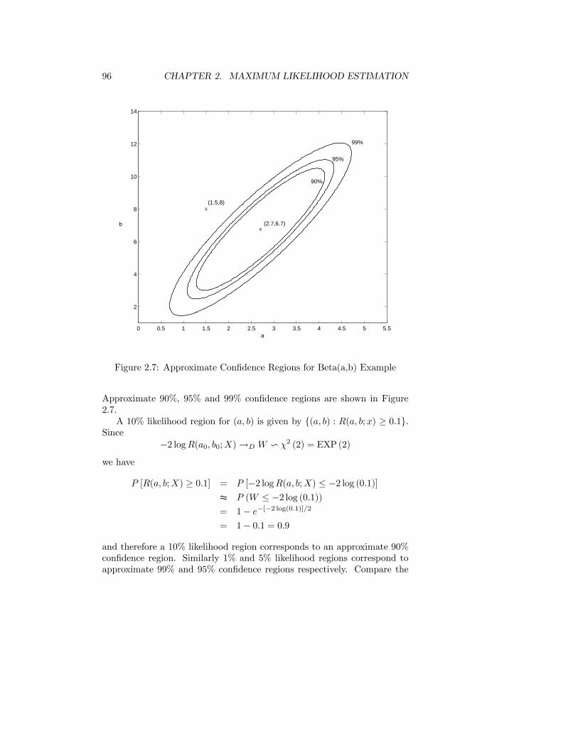
96 CHAPTER 2. MAXIMUM LIKELIHOOD ESTIMATION
(2.7,6.7)
(1.5,8)
a
b
90%
95%
99%
0 0.5 1 1.5 2 2.5 3 3.5 4 4.5 5 5.5
2
4
6
8
10
12
14
Figure 2.7: Approximate Confidence Regions for Beta(a,b) Example
Approximate 90%, 95% and 99% confidence regions are shown in Figure2.7.A 10% likelihood region for (a, b) is given by (a, b) : R(a, b;x) ≥ 0.1.
Since
−2 logR(a0, b0;X)→D W v χ2 (2) = EXP (2)
we have
P [R(a, b;X) ≥ 0.1] = P [−2 logR(a, b;X) ≤ −2 log (0.1)]≈ P (W ≤ −2 log (0.1))= 1− e−[−2 log(0.1)]/2
= 1− 0.1 = 0.9
and therefore a 10% likelihood region corresponds to an approximate 90%confidence region. Similarly 1% and 5% likelihood regions correspond toapproximate 99% and 95% confidence regions respectively. Compare the
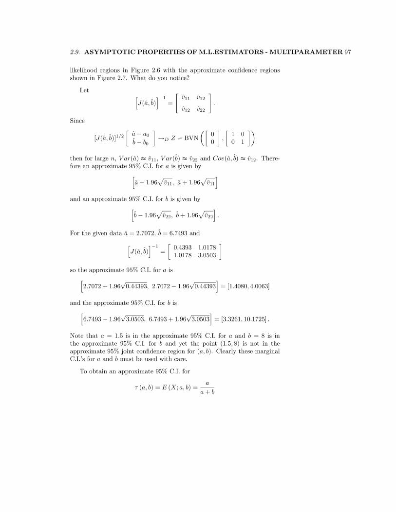
2.9. ASYMPTOTIC PROPERTIES OFM.L.ESTIMATORS - MULTIPARAMETER 97
likelihood regions in Figure 2.6 with the approximate confidence regionsshown in Figure 2.7. What do you notice?
Let hJ(a, b)
i−1=
"v11 v12
v12 v22
#.
Since
[J(a, b)]1/2∙a− a0b− b0
¸→D Z v BVN
µ∙00
¸,
∙1 00 1
¸¶then for large n, V ar(a) ≈ v11, V ar(b) ≈ v22 and Cov(a, b) ≈ v12. There-fore an approximate 95% C.I. for a is given byh
a− 1.96pv11, a+ 1.96
pv11
iand an approximate 95% C.I. for b is given byh
b− 1.96pv22, b+ 1.96
pv22
i.
For the given data a = 2.7072, b = 6.7493 andhJ(a, b)
i−1=
∙0.4393 1.01781.0178 3.0503
¸so the approximate 95% C.I. for a ish
2.7072 + 1.96√0.44393, 2.7072− 1.96
√0.44393
i= [1.4080, 4.0063]
and the approximate 95% C.I. for b ish6.7493− 1.96
√3.0503, 6.7493 + 1.96
√3.0503
i= [3.3261, 10.1725] .
Note that a = 1.5 is in the approximate 95% C.I. for a and b = 8 is inthe approximate 95% C.I. for b and yet the point (1.5, 8) is not in theapproximate 95% joint confidence region for (a, b). Clearly these marginalC.I.’s for a and b must be used with care.
To obtain an approximate 95% C.I. for
τ (a, b) = E (X; a, b) =a
a+ b
98 CHAPTER 2. MAXIMUM LIKELIHOOD ESTIMATION
we use (2.13) with
D (a, b) =£
∂τ∂a
∂τ∂b
¤T=h
b(a+b)2
−a(a+b)2
iTand
v = [D(a, b)]T [J(a, b)]−1D(a, b)
=h
b(a+b)2
−a(a+b)2
i " v11 v12
v12 v22
#"b
(a+b)2−a
(a+b)2
#
For the given data
τ(a, b) =a
a+ b=
2.7072
2.7072 + 6.7493= 0.28628
andv = 0.00064706.
The approximate 95% C.I. for τ (a, b) = E (X; a, b) = a/ (a+ b) ish0.28628− 1.96
√0.00064706, 0.28628 + 1.96
√0.00064706
i= [0.23642, 0.33614] .
2.9.4 Problem
In Problem 2.4.10 find an approximate 95% C.I. for Cov(X1,X2; θ1, θ2).
2.9.5 Problem
In Problem 2.4.18 find an approximate 95% joint confidence region for (α,β)and approximate 95% C.I.’s for β and τ(α,β) = E(X;α,β) = αβ.
2.9.6 Problem
In Problem 2.4.19 find approximate 95% C.I.’s for β and E(X;α,β).
2.9.7 Problem
Suppose X1, ...,Xn is a random sample from the EXP(β,μ) distribution.
Show that the M.L. estimators βn and μn are consistent estimators. Howwould you construct a joint confidence region for (β,μ)? How would youconstruct a C.I. for β? How would you construct a C.I. for μ?
2.9. ASYMPTOTIC PROPERTIES OFM.L.ESTIMATORS - MULTIPARAMETER 99
2.9.8 Problem
Consider the model in Problem 1.7.26. Explain clearly how you wouldconstruct a C.I. for σ2 and a C.I. for μ.
2.9.9 Problem
Let X1, . . . ,Xn be a random sample from the distribution with p.d.f.
f (x;α,β) =αxα−1
βα, 0 < x ≤ β, α > 0.
(a) Find the likelihood function of α and β and the M.L. estimators of αand β.
(b) Show that the M.L. estimator of α is a consistent estimator of α. Showthat the M.L. estimator of β is a consistent estimator of β.
(c) If n = 15, x(15) = 0.99 and15Pi=1log xi = −7.7685 find the M.L. estimates
of α and β.
(d) If n = 15, x(15) = 0.99 and15Pi=1log xi = −7.7685, construct an exact
95% equal-tail C.I. for α and an exact 95% one-tail C.I. for β.
(e) Explain how you would construct a joint likelihood region for α and β.Explain how you would construct a joint confidence region for α and β?
2.9.10 Problem
The following are the results, in millions of revolutions to failure, of en-durance tests for 23 deep-groove ball bearings:
17.88 28.92 33.00 41.52 42.12 45.6048.48 51.84 51.96 54.12 55.56 67.8068.64 68.64 68.88 84.12 93.12 98.64105.12 105.84 127.92 128.04 173.40
As a result of testing thousands of ball bearings, it is known that theirlifetimes have a WEI(θ,β) distribution.
(a) Find the M.L. estimates of θ and β and the observed information I(θ, β).
(b) Plot the 1%, 5% and 10% likelihood regions for θ and β on the samegraph.
100 CHAPTER 2. MAXIMUM LIKELIHOOD ESTIMATION
(c) Plot the approximate 99%, 95% and 90% joint confidence regions for θand β on the same graph. Compare these with the likelihood regions in (b)and comment.
(d) Calulate an approximate 95% confidence interval for β.
(e) The value β = 1 is of interest since WEI(θ, 1) = EXP (θ). Is β = 1 aplausible value of β in light of the observed data? Justify your conclusion.
(f) If X vWEI (θ,β) then
P (X > 80; θ,β) = exp
"−µ80
θ
¶β#= τ (θ,β) .
Find an approximate 95% confidence interval for τ (θ,β).
2.9.11 Example - Logistic Regression
Pistons are made by casting molten aluminum into moulds and then ma-chining the raw casting. One defect that can occur is called porosity, dueto the entrapment of bubbles of gas in the casting as the metal solidifies.The presence or absence of porosity is thought to be a function of pouringtemperature of the aluminum.One batch of raw aluminum is available and the pistons are cast in 8
different dies. The pouring temperature is set at one of 4 levels
750, 775, 800, 825
and at each level, 3 pistons are cast in the 8 dies available. The presence(1) or absence (0) of porosity is recorded for each piston and the data aregiven below:
Temperature Total
750 0 0 1 0 1 0 1 1 0 1 1 01 1 0 1 0 0 1 0 1 0 1 1 13
775 0 0 1 0 0 0 1 1 1 1 1 10 0 1 0 1 0 0 1 0 0 1 0 11
800 0 0 0 1 0 1 1 0 0 0 0 01 0 1 1 0 0 1 1 1 0 0 1 10
825 0 0 0 1 0 0 1 1 0 1 1 10 0 0 0 0 0 0 0 1 0 1 0 8
In Figure 2.8, the scatter plot of the proportion of pistons with porosityversus temperature shows that there is a general decrease in porosity astemperature increases.
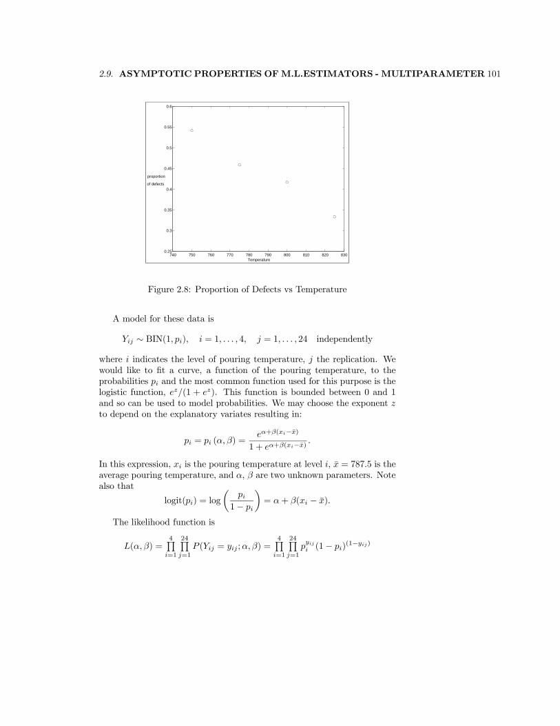
2.9. ASYMPTOTIC PROPERTIES OFM.L.ESTIMATORS - MULTIPARAMETER 101
740 750 760 770 780 790 800 810 820 8300.25
0.3
0.35
0.4
0.45
0.5
0.55
0.6
Temperature
proportion
of defects
Figure 2.8: Proportion of Defects vs Temperature
A model for these data is
Yij ∼ BIN(1, pi), i = 1, . . . , 4, j = 1, . . . , 24 independently
where i indicates the level of pouring temperature, j the replication. Wewould like to fit a curve, a function of the pouring temperature, to theprobabilities pi and the most common function used for this purpose is thelogistic function, ez/(1 + ez). This function is bounded between 0 and 1and so can be used to model probabilities. We may choose the exponent zto depend on the explanatory variates resulting in:
pi = pi (α,β) =eα+β(xi−x)
1 + eα+β(xi−x).
In this expression, xi is the pouring temperature at level i, x = 787.5 is theaverage pouring temperature, and α, β are two unknown parameters. Notealso that
logit(pi) = log
µpi
1− pi
¶= α+ β(xi − x).
The likelihood function is
L(α,β) =4Qi=1
24Qj=1
P (Yij = yij ;α,β) =4Qi=1
24Qj=1
pyiji (1− pi)(1−yij)
102 CHAPTER 2. MAXIMUM LIKELIHOOD ESTIMATION
and the log likelihood is
l (α,β) =4Pi=1
24Pj=1
[yij log (pi) + (1− yij) log (1− pi)] .
Note that∂pi∂α
= pi (1− pi)
and∂pi∂β
= (xi − x) pi (1− pi)
so that
∂l(α,β)
∂α=
4Pi=1
24Pj=1
∂l
∂pi· ∂pi∂α
=4Pi=1
24Pj=1
∙yijpi− 1− yij1− pi
¸pi (1− pi)
=4Pi=1
24Pj=1
[yij (1− pi)− (1− yij) pi] =4Pi=1
24Pj=1
(yij − pi)
=4Pi=1(yi. − 24pi)
where
yi. =24Pj=1
yij .
Similarly∂l(α,β)
∂β=
4Pi=1(xi − x)(yi. − 24pi).
The score function is
S(α,β) =
⎡⎢⎢⎢⎣4Pi=1(yi. − 24pi)
4Pi=1(xi − x)(yi. − 24pi)
⎤⎥⎥⎥⎦ .Since
∂2l (α,β)
∂α2= 24
4Pi=1
∂pi∂α
= 244Pi=1pi (1− pi) ,
∂2l (α,β)
∂β2= 24
4Pi=1(xi − x)
∂pi∂β
= 244Pi=1(xi − x)2 pi (1− pi) ,
and∂2l (α,β)
∂α∂β= 24
4Pi=1
∂pi∂β
= 244Pi=1(xi − x) pi (1− pi)
2.9. ASYMPTOTIC PROPERTIES OFM.L.ESTIMATORS - MULTIPARAMETER 103
the information matrix and the Fisher information matrix are equal andgiven by
I (α,β) = J (α,β) =
⎡⎢⎢⎢⎣24
4Pi=1pi (1− pi) 24
4Pi=1(xi − x)pi(1− pi)
244Pi=1(xi − x)pi(1− pi) 24
4Pi=1(xi − x)2 pi (1− pi)
⎤⎥⎥⎥⎦ .
To find the M.L. estimators of α and β we must solve
∂l(α,β)
∂α= 0 =
∂l(α,β)
∂β
simultaneously which must be done numerically using a method such asNewton’s method. Initial estimates of α and β can be obtained by drawinga line through the points in Figure 2.8, choosing two points on the line andthen solving for α and β. For example, suppose we require that the linepass through the points (775, 11/24) and (825, 8/24). We obtain
−0.167 = logit(11/24) = α+ β (775− 787.5) = α+ β(−12.5)
−0.693 = logit(8/24) = α+ β (825− 787.5) = α+ β(37.5),
and these result in initial estimates: α(0) = −0.298, β(0) = −0.0105.Now
J³α(0),β(0)
´=
∙23.01 −27.22−27.22 17748.30
¸and
S³α(0),β(0)
´= [0.9533428, − 9.521179]T
and the first iteration of Newton’s method gives∙α(1)
β(1)
¸=
∙α(0)
β(0)
¸+hJ³α(0),β(0)
´i−1S³α(0),β(0)
´=
∙−0.2571332−0.01097377
¸.
Repeating this process does not substantially change these estimates, so wehave the M.L. estimates:
α = −0.2571831896 β = −0.01097623887.
The Fisher information matrix evaluated at the M.L. estimate is
J(α, β) =
"23.09153 −24.63342−24.63342 17783.63646
#.
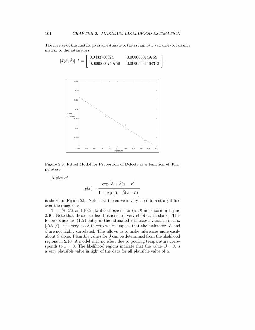
104 CHAPTER 2. MAXIMUM LIKELIHOOD ESTIMATION
The inverse of this matrix gives an estimate of the asymptotic variance/covariancematrix of the estimators:
[J(α, β)]−1 =
"0.0433700024 0.0000600749759
0.0000600749759 0.00005631468312
#.
740 750 760 770 780 790 800 810 820 830 840
0.35
0.4
0.45
0.5
0.55
0.6
0.65
Temperature
proportion
of defects
Figure 2.9: Fitted Model for Proportion of Defects as a Function of Tem-perature
A plot of
p(x) =exp
hα+ β(x− x)
i1 + exp
hα+ β(x− x)
iis shown in Figure 2.9. Note that the curve is very close to a straight lineover the range of x.The 1%, 5% and 10% likelihood regions for (α,β) are shown in Figure
2.10. Note that these likelihood regions are very elliptical in shape. Thisfollows since the (1, 2) entry in the estimated variance/covariance matrix
[J(α, β)]−1 is very close to zero which implies that the estimators α and
β are not highly correlated. This allows us to make inferences more easilyabout β alone. Plausible values for β can be determined from the likelihoodregions in 2.10. A model with no effect due to pouring temperature corre-sponds to β = 0. The likelihood regions indicate that the value, β = 0, isa very plausible value in light of the data for all plausible value of α.
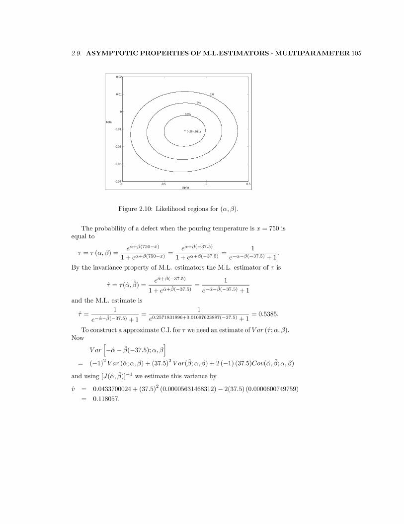
2.9. ASYMPTOTIC PROPERTIES OFM.L.ESTIMATORS - MULTIPARAMETER 105
alpha
(-.26,-.011)
10%
5%
1%
beta
-1 -0.5 0 0.5-0.04
-0.03
-0.02
-0.01
0
0.01
0.02
Figure 2.10: Likelihood regions for (α,β).
The probability of a defect when the pouring temperature is x = 750 isequal to
τ = τ (α,β) =eα+β(750−x)
1 + eα+β(750−x)=
eα+β(−37.5)
1 + eα+β(−37.5)=
1
e−α−β(−37.5) + 1.
By the invariance property of M.L. estimators the M.L. estimator of τ is
τ = τ(α, β) =eα+β(−37.5)
1 + eα+β(−37.5)=
1
e−α−β(−37.5) + 1
and the M.L. estimate is
τ =1
e−α−β(−37.5) + 1=
1
e0.2571831896+0.01097623887(−37.5) + 1= 0.5385.
To construct a approximate C.I. for τ we need an estimate of V ar (τ ;α,β).Now
V arh−α− β(−37.5);α,β
i= (−1)2 V ar (α;α,β) + (37.5)2 V ar(β;α,β) + 2 (−1) (37.5)Cov(α, β;α,β)
and using [J(α, β)]−1 we estimate this variance by
v = 0.0433700024 + (37.5)2 (0.00005631468312)− 2(37.5) (0.0000600749759)= 0.118057.
106 CHAPTER 2. MAXIMUM LIKELIHOOD ESTIMATION
An approximate 95% C.I. for −α− β(−37.5) is
[−α− β(−37.5)− 1.96√v, − α− β(−37.5) + 1.96
√v]
=h−0.154426− 1.96
√0.118057, − 0.154426 + 1.96
√0.118057
i= [−0.827870, 0.519019] .
An approximate 95% C.I. for
τ = τ (α,β) =1
e−α−β(−37.5) + 1
is ∙1
exp (0.519019) + 1,
1
exp (−0.827870) + 1
¸= [0.373082, 0.695904] .
The near linearity of the fitted function as indicated in Figure 2.9 seemsto imply that we need not use the logistic function treated in this example,but that a straight line could have been fit to these data with similar resultsover the range of temperatures observed. Indeed, a simple linear regressionwould provide nearly the same fit. However, if values of pi near 0 or 1 hadbeen observed, e.g. for temperatures well above or well below those usedhere, the non-linearity of the logistic function would have been importantand provided some advantage over simple linear regression.
2.9.12 Problem - The Challenger Data
On January 28, 1986, the twenty-fifth flight of the U.S. space shuttle pro-gram ended in disaster when one of the rocket boosters of the ShuttleChallenger exploded shortly after lift-off, killing all seven crew members.The presidential commission on the accident concluded that it was causedby the failure of an O-ring in a field joint on the rocket booster, and thatthis failure was due to a faulty design that made the O-ring unacceptablysensitive to a number of factors including outside temperature. Of the pre-vious 24 flights, data were available on failures of O-rings on 23, (one waslost at sea), and these data were discussed on the evening preceding theChallenger launch, but unfortunately only the data corresponding to the7 flights on which there was a damage incident were considered importantand these were thought to show no obvious trend. The data are given inTable 1. (See Dalal, Fowlkes and Hoadley (1989), JASA, 84, 945-957.)
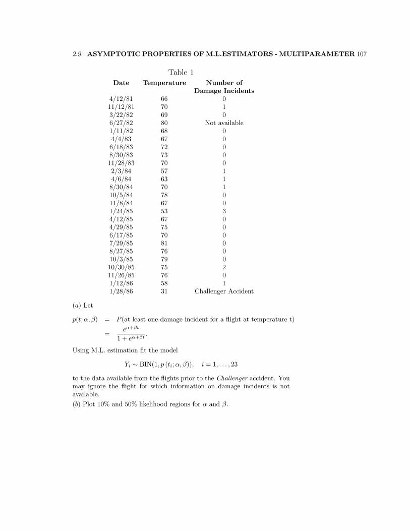
2.9. ASYMPTOTIC PROPERTIES OFM.L.ESTIMATORS - MULTIPARAMETER 107
Table 1Date Temperature Number of
Damage Incidents4/12/81 66 011/12/81 70 13/22/82 69 06/27/82 80 Not available1/11/82 68 04/4/83 67 06/18/83 72 08/30/83 73 011/28/83 70 02/3/84 57 14/6/84 63 18/30/84 70 110/5/84 78 011/8/84 67 01/24/85 53 34/12/85 67 04/29/85 75 06/17/85 70 07/29/85 81 08/27/85 76 010/3/85 79 010/30/85 75 211/26/85 76 01/12/86 58 11/28/86 31 Challenger Accident
(a) Let
p(t;α,β) = P (at least one damage incident for a flight at temperature t)
=eα+βt
1 + eα+βt.
Using M.L. estimation fit the model
Yi ∼ BIN(1, p (ti;α,β)), i = 1, . . . , 23
to the data available from the flights prior to the Challenger accident. Youmay ignore the flight for which information on damage incidents is notavailable.
(b) Plot 10% and 50% likelihood regions for α and β.
108 CHAPTER 2. MAXIMUM LIKELIHOOD ESTIMATION
(c) Find an approximate 95% C.I. for β. How plausible is the value β = 0?
(d) Find an approximate 95% C.I. for p(t) if t = 31, the temperature onthe day of the disaster. Comment.
2.10 Nuisance Parameters andM.L. Estimation
Suppose X1, . . . ,Xn is a random sample from the distribution with proba-bility (density) function f (x; θ). Suppose also that θ = (λ,φ) where λ is avector of parameters of interest and φ is a vector of nuisance parameters.The profile likelihood is one modification of the likelihood which allows
us to look at estimation methods for λ in the presence of the nuisanceparameter φ.
2.10.1 Definition
Suppose θ = (λ,φ) with likelihood function L(λ,φ). Let φ(λ) be the M.L.estimator of φ for a fixed value of λ. Then the profile likelihood for λ isgiven by L(λ, φ(λ)).
The M.L. estimator of λ based on the profile likelihood is, of course,the same estimator obtained by maximizing the joint likelihood L(λ,φ)simultaneously over λ and φ. If the profile likelihood is used to constructlikelihood regions for λ, care must be taken since the imprecision in theestimation of the nuisance paramter φ is not taken into account.Profile likelihood is one example of a group of modifications of the like-
lihood known as pseudo-likelihoods which are based on a derived likelihoodfor a subset of parmeters. Marginal likelihood, conditional likelihood andpartial likelihood are also included in this class.Suppose that θ = (λ,φ) and the data X, or some function of the data,
can be partitioned into U and V . Suppose also that
f(u, v; θ) = f(u;λ) · f(v|u; θ).
If the conditional distribution of V given U does depends only on φ thenestimation of λ can be based on f(u;λ), the marginal likelihood for λ. Iff(v|u; θ) depends on both λ and φ then the marginal likelihood may still beused for estimation of λ if, in ignoring the conditional distribution, there islittle information lost.If there is a factorization of the form
f(u, v; θ) = f(u|v;λ) · f(v; θ)
2.11. PROBLEMS WITH M.L. ESTIMATORS 109
then estimation of λ can be based on f(u|v;λ) the conditional likelihoodfor λ.
2.10.2 Problem
Suppose X1, . . . ,Xn is a random sample from a N(μ,σ2) distribution andthat σ is the parameter of interest while μ is a nuisance parameter. Find theprofile likelihood of σ. Let U = S2 and V = X. Find f(u;σ), the marginallikelihood of σ and f(u|v;σ), the conditional likelihood of σ. Compare thethree likelihoods.
2.11 Problems with M.L. Estimators
2.11.1 Example
This is an example to indicate that in the presence of a large number ofnuisance parameters, it is possible for a M.L. estimator to be inconsistent.Suppose we are interested in the effect of environment on the performance ofidentical twins in some test, where these twins were separated at birth andraised in different environments. If the vector (Xi, Yi) denotes the scoresof the i’th pair of twins, we might assume (Xi, Yi) are both independentN(μi,σ
2) random variables. We wish to estimate the parameter σ2 basedon a sample of n twins. Show that the M.L. estimator of σ2 is
σ2 = 14n
nPi=1
(Xi − Yi)2 and this is a biased and inconsistent estimator of
σ2. Show, however, that a simple modification results in an unbiased andconsistent estimator.
2.11.2 Example
Recall that Theorem 2.7.2 states that under some conditions a root of thelikelihood equation exists which is consistent as the sample size approachesinfinity. One might wonder why the theorem did not simply make the sameassertion for the value of the parameter providing the global maximum ofthe likelihood function. The answer is that while the consistent root ofthe likelihood equation often corresponds to the global maximum of thelikelihood function, there is no guarantee of this without some additionalconditions. This somewhat unusual example shows circumstances underwhich the consistent root of the likelihood equation is not the global maxi-mizer of the likelihood function. Suppose Xi, i = 1, . . . , n are independent
110 CHAPTER 2. MAXIMUM LIKELIHOOD ESTIMATION
observations from the mixture density of the form
f (x; θ) =²√2πσ
e−(x−μ)2/2σ2 +
1− ²√2πe−(x−μ)
2/2
where θ = (μ,σ2) with both parameters unknown. Notice that the likeli-hood function L(μ,σ) → ∞ for μ = xj ,σ → 0 for any j = 1, . . . , n. Thismeans that the globally maximizing σ is σ = 0, which lies on the boundaryof the parameter space. However, there is a local maximum of the likeli-hood function at some σ > 0 which provides a consistent estimator of theparameter.
2.11.3 Unidentifiability and Singular Information Ma-trices
Suppose we observe two independent random variables Y1, Y2 having nor-mal distributions with the same variance σ2 and means θ1 + θ2, θ2 + θ3respectively. In this case, although the means depend on the parameterθ = (θ1, θ2, θ3), the value of this vector parameter is unidentifiable in thesense that, for some pairs of distinct parameter values, the probability den-sity function of the observations are identical. For example the parameterθ = (1, 0, 1) leads to exactly the same joint distribution of Y1, Y2 as doesthe parameter θ = (0, 1, 0). In this case, we we might consider only thetwo parameters (φ1,φ2) = (θ1 + θ2, θ2 + θ3) and anything derivable fromthis pair estimable, while parameters such as θ2 that cannot be obtainedas functions of φ1,φ2 are consequently unidentifiable. The solution to theoriginal identifiability problem is the reparametrization to the new para-meter (φ1,φ2) in this case, and in general, unidentifiability usually meansone should seek a new, more parsimonious parametrization.
In the above example, compute the Fisher information matrix for theparameter θ = (θ1, θ2, θ3). Notice that the Fisher information matrix issingular. This means that if you were to attempt to compute the asymptoticvariance of the M.L. estimator of θ by inverting the Fisher informationmatrix, the inversion would be impossible. Attempting to invert a singularmatrix is like attempting to invert the number zero. It results in one ormore components that you can consider to be infinite. Arguing intuitively,the asymptotic variance of the M.L. estimator of some of the parametersis infinite. This is an indication that asymptotically, at least, some of theparameters may not be identifiable. When parameters are unidentifiable,the Fisher information matrix is generally singular. However, when J(θ)is singular for all values of θ, this may or may not mean parameters areunidentifiable for finite sample sizes, but it does usually mean one should
2.12. HISTORICAL NOTES 111
take a careful look at the parameters with a possible view to adoptinganother parametrization.
2.11.4 U.M.V.U.E.’s and M.L. Estimators: A Com-parison
Should we use U.M.V.U.E.’s or M.L. estimators? There is no general con-sensus among statisticians.
1. If we are estimating the expectation of a natural sufficient statisticTi(X) in a regular exponential family both M.L. and unbiasednessconsiderations lead to the use of Ti as an estimator.
2. When sample sizes are large U.M.V.U.E.’s and M.L. estimators areessentially the same. In that case use is governed by ease of compu-tation. Unfortunately how large “large” needs to be is usually un-known. Some studies have been carried out comparing the behaviourof U.M.V.U.E.’s and M.L. estimators for various small fixed samplesizes. The results are, as might be expected, inconclusive.
3. M.L. estimators exist “more frequently” and when they do they areusually easier to compute than U.M.V.U.E.’s. This is essentially be-cause of the appealing invariance property of M.L.E.’s.
4. Simple examples are known for which M.L. estimators behave badlyeven for large samples (see Examples 2.10.1 and 2.10.2 above).
5. U.M.V.U.E.’s and M.L. estimators are not necessarily robust. Theyare sensitive to model misspecification.
In Chapter 3 we examine other approaches to estimation.
2.12 Historical Notes
The concept of sufficiency is due to Fisher (1920), who in his fundamentalpaper of 1922 also introduced the term and stated the factorization crite-rion. The criterion was rediscovered by Neyman (1935) and was provedfor general dominated families by Halmos and Savage (1949). The the-ory of minimal sufficiency was initiated by Lehmann and Scheffe (1950)and Dynkin (1951). For further generalizations, see Bahadur (1954) andLanders and Rogge (1972).One-parameter exponential families as the only (regular) families of dis-
tributions for which there exists a one-dimensional sufficient statistic were
112 CHAPTER 2. MAXIMUM LIKELIHOOD ESTIMATION
also introduced by Fisher (1934). His result was generalized to more thanone dimension by Darmois (1935), Koopman (1936) and Pitman (1936). Amore recent discussion of this theorem with references to the literature isgiven, for example, by Hipp (1974). A comprehensive treatment of expo-nential families is provided by Barndorff-Nielsen (1978).The concept of unbiasedness as “lack of systematic error” in the esti-
mator was introduced by Gauss (1821) in his work on the theory of leastsquares. The first UMVU estimators were obtained by Aitken and Silver-stone (1942) in the situation in which the information inequality yields thesame result. UMVU estimators as unique unbiased functions of a suitablesufficient statistic were derived in special cases by Halmos (1946) and Kol-mogorov (1950), and were pointed out as a general fact by Rao (1947). Theconcept of completeness was defined, its implications for unbiased estima-tion developed, and the Lehmann-Scheffe Theorem obtained in Lehmannand Scheffe (1950, 1955, 1956). Basu’s theorem is due to Basu (1955, 1958).The origins of the concept of maximum likelihood go back to the work
of Lambert, Daniel Bernoulli, and Lagrange in the second half of the 18thcentury, and of Gauss and Laplace at the beginning of the 19th. [Fordetails and references, see Edwards (1974).] The modern history beginswith Edgeworth (1908-09) and Fisher (1922, 1925), whose contributionsare discussed by Savage (1976) and Pratt (1976).The amount of information that a data set contains about a parameter
was introduced by Edgeworth (1908, 1909) and was developed systemati-cally by Fisher (1922 and later papers). The first version of the informationinequality appears to have been given by Frechet (1943), Rao (1945), andCramer (1946). The designation “information inequality” which replacedthe earlier “Cramer-Rao inequality” was proposed by Savage (1954).Fisher’s work on maximum likelihood was followed by a euphoric belief
in the universal consistence and asymptotic efficiency of maximum likeli-hood estimators, at least in the i.i.d. case. The true situation was sortedout gradually. Landmarks are Wald (1949), who provided fairly generalconditions for consistency, Cramer (1946), who defined the “regular” casein which the likelihood equation has a consistent asymptotically efficientroot, the counterexamples of Bahadur (1958) and Hodges (Le Cam, 1953),and Le Cam’s resulting theorem on superefficiency (1935).
Chapter 3
Other Methods ofEstimation
3.1 Best Linear Unbiased Estimators
The problem of finding best unbiased estimators is considerably simpler ifwe limit the class in which we search. If we permit any function of thedata, then we usually require the heavy machinery of complete sufficiencyto produce U.M.V.U.E.’s. However, the situation is much simpler if wesuggest some initial random variables and then require that our estimatorbe a linear combination of these. Suppose, for example we have randomvariables Y1, Y2, Y3 with E(Y1) = α + θ, E(Y2) = α − θ, E(Y3) = θ whereθ is the parameter of interest and α is another parameter. What linearcombinations of the Yi’s provide an unbiased estimator of θ and among thesepossible linear combinations which one has the smallest possible variance?To answer these questions, we need to know the covariances Cov(Yi, Yj)(at least up to some scalar multiple). Suppose Cov(Yi, Yj) = 0, i 6= j andV ar(Yj) = σ2. Let Y = (Y1, Y2, Y3)
T and β = (α, θ)T . The model can bewritten as a general linear model as
Y = Xβ + ²
where
X =
⎡⎣ 1 11 −10 1
⎤⎦ ,ε = (ε1, ε2, ε3)
T , and the εi’s are uncorrelated random variables withE(²i) = 0 and V ar(εi) = σ2. Then the linear combination of the compo-
113
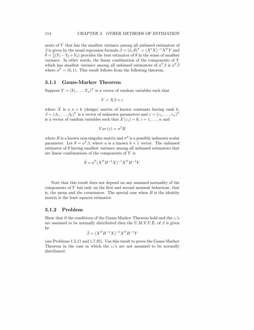
114 CHAPTER 3. OTHER METHODS OF ESTIMATION
nents of Y that has the smallest variance among all unbiased estimators ofβ is given by the usual regression formula β = (α, θ)T = (XtX)−1XTY andθ = 1
3(Y1−Y2+Y3) provides the best estimator of θ in the sense of smallestvariance. In other words, the linear combination of the components of Ywhich has smallest variance among all unbiased estimators of aTβ is aT βwhere aT = (0, 1). This result follows from the following theorem.
3.1.1 Gauss-Markov Theorem
Suppose Y = (Y1, . . . , Yn)T is a vector of random variables such that
Y = Xβ + ε
where X is a n × k (design) matrix of known constants having rank k,β = (β1, . . . ,βk)
T is a vector of unknown parameters and ε = (ε1, . . . , εn)T
is a vector of random variables such that E (εi) = 0, i = 1, . . . , n and
V ar (ε) = σ2B
whereB is a known non-singular matrix and σ2 is a possibly unknown scalarparameter. Let θ = aTβ, where a is a known k × 1 vector. The unbiasedestimator of θ having smallest variance among all unbiased estimators thatare linear combinations of the components of Y is
θ = aT (XTB−1X)−1XTB−1Y.
Note that this result does not depend on any assumed normality of thecomponents of Y but only on the first and second moment behaviour, thatis, the mean and the covariances. The special case when B is the identitymatrix is the least squares estimator.
3.1.2 Problem
Show that if the conditions of the Gauss-Markov Theorem hold and the εi’sare assumed to be normally distributed then the U.M.V.U.E. of β is givenby
β = (XTB−1X)−1XTB−1Y
(see Problems 1.5.11 and 1.7.25). Use this result to prove the Gauss-MarkovTheorem in the case in which the εi’s are not assumed to be normallydistributed.
3.2. EQUIVARIANT ESTIMATORS 115
3.1.3 Example
Suppose T1, . . . , Tn are independent unbiased estimators of θ with knownvariances V ar(Ti) = σ2i , i = 1, . . . , n. Find the best linear combination ofthese estimators, that is, the one that results in an unbiased estimator of θhaving the minimum variance among all linear unbiased estimators.
3.1.4 Problem
Suppose Yij , i = 1, 2; j = 1, . . . , n are independent random variables withE(Yij) = μ+ αi and V ar(Yij) = σ2 where α1 + α2 = 0.
(a) Find the best linear unbiased estimator of α1.
(b) Under what additional assumptions is this estimator the U.M.V.U.E.?Justify your answer.
3.1.5 Problem
Suppose Yij , i = 1, 2; j = 1, . . . , ni are independent random variables with
E (Yij) = αi + βi (xij − xi) , V ar (Yij) = σ2 and xi =1
ni
niPj=1
xij .
(a) Find the best linear unbiased estimators of α1, α2, β1 and β2.
(b) Under what additional assumptions are these estimators the U.M.V.U.E.’s?Justify your answer.
3.1.6 Problem
Suppose X1, . . . ,Xn is a random sample from the N(μ,σ2) distribution.Find the linear combination of the random variables (Xi−X)2, i = 1, . . . , nwhich minimizes the M.S.E. for estimating σ2. Compare this estimator withthe M.L. estimator and the U.M.V.U.E. of σ2.
3.2 Equivariant Estimators
3.2.1 Definition
A model f (x; θ) ; θ ∈ < such that f (x; θ) = f0(x− θ) with f0 known iscalled a location invariant family and θ is called a location parameter. (See1.2.3.)
In many examples the location of the origin is arbitrary. For exampleif we record temperatures in degrees celcius, the 0 point has been more or
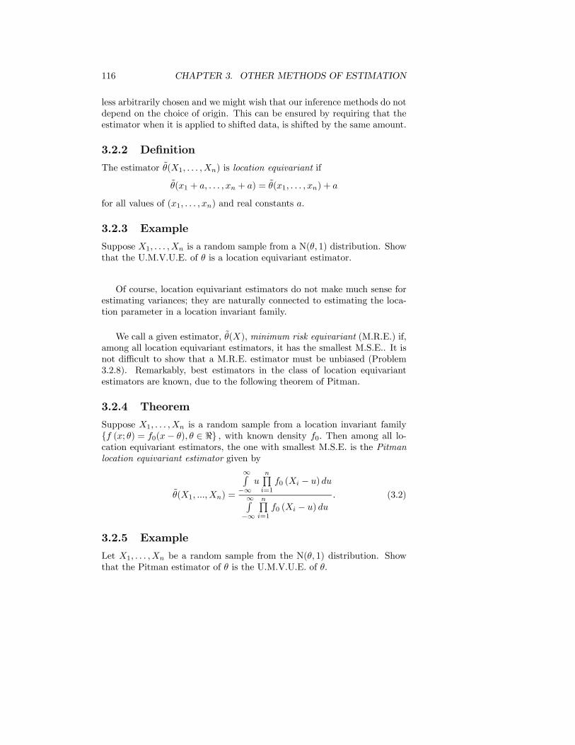
116 CHAPTER 3. OTHER METHODS OF ESTIMATION
less arbitrarily chosen and we might wish that our inference methods do notdepend on the choice of origin. This can be ensured by requiring that theestimator when it is applied to shifted data, is shifted by the same amount.
3.2.2 Definition
The estimator θ(X1, . . . ,Xn) is location equivariant if
θ(x1 + a, . . . , xn + a) = θ(x1, . . . , xn) + a
for all values of (x1, . . . , xn) and real constants a.
3.2.3 Example
Suppose X1, . . . ,Xn is a random sample from a N(θ, 1) distribution. Showthat the U.M.V.U.E. of θ is a location equivariant estimator.
Of course, location equivariant estimators do not make much sense forestimating variances; they are naturally connected to estimating the loca-tion parameter in a location invariant family.
We call a given estimator, θ(X), minimum risk equivariant (M.R.E.) if,among all location equivariant estimators, it has the smallest M.S.E.. It isnot difficult to show that a M.R.E. estimator must be unbiased (Problem3.2.8). Remarkably, best estimators in the class of location equivariantestimators are known, due to the following theorem of Pitman.
3.2.4 Theorem
Suppose X1, . . . ,Xn is a random sample from a location invariant familyf (x; θ) = f0(x− θ), θ ∈ < , with known density f0. Then among all lo-cation equivariant estimators, the one with smallest M.S.E. is the Pitmanlocation equivariant estimator given by
θ(X1, ...,Xn) =
∞R−∞
unQi=1f0 (Xi − u) du
∞R−∞
nQi=1f0 (Xi − u) du
. (3.2)
3.2.5 Example
Let X1, . . . ,Xn be a random sample from the N(θ, 1) distribution. Showthat the Pitman estimator of θ is the U.M.V.U.E. of θ.
3.2. EQUIVARIANT ESTIMATORS 117
3.2.6 Problem
Prove that the M.R.E. estimator is unbiased.
3.2.7 Problem
Let (X1,X2) be a random sample from the distribution with probabilitydensity function
f (x; θ) = −6(x− θ − 12)(x− θ +
1
2), θ − 1
2< x < θ +
1
2.
Show that the Pitman estimator of θ is θ (X1,X2) = (X1 +X2)/2.
3.2.8 Problem
Let X1, . . . ,Xn be a random sample from the EXP(1, θ) distribution. Findthe Pitman estimator of θ and compare it to the M.L. estimator of θ andthe U.M.V.U.E. of θ.
3.2.9 Problem
Let X1, . . . ,Xn be a random sample from the UNIF(θ − 1/2, θ + 1/2) dis-tribution. Find the Pitman estimator of θ. Show that the M.L. estimatoris not unique in this case.
3.2.10 Problem
Suppose X1, . . . ,Xn is a random sample from a location invariant familyf (x; θ) = f0(x− θ), θ ∈ <. Show that if the M.L. estimator is uniquethen it is a location equivariant estimator.
Since the M.R.E. estimator is an unbiased estimator, it follows thatif there is a U.M.V.U.E. in a given problem and if that U.M.V.U.E. islocation equivariant then the M.R.E. estimator and the U.M.V.U.E. mustbe identical. M.R.E. estimators are primarily used when no U.M.V.U.E.exists. For example, the Pitman estimator of the location parameter fora Cauchy distribution performs very well by comparison with any otherestimator, including the M.L. estimator.
3.2.11 Definition
A model f (x; θ) ; θ > 0 such that f (x; θ) = 1θf1(
xθ ) with f1 known is
called a scale invariant family and θ is called a scale parameter (See 1.2.3).
118 CHAPTER 3. OTHER METHODS OF ESTIMATION
3.2.12 Definition
An estimator θk = θk(X1, . . . ,Xn) is scale equivariant if
θk(cx1, . . . , cxn) = ckθk(x1, . . . , xn)
for all values of (x1, . . . , xn) and c > 0.
3.2.13 Theorem
Suppose X1, . . . ,Xn is a random sample from a scale invariant family©f (x; θ) = 1
θf1(xθ ), θ > 0
ª, with known density f1. The Pitman scale equivari-
ant estimator of θk which minimizes
E
⎡⎣Ã θk − θk
θk
!2; θ
⎤⎦(the scaled M.S.E.) is given by
θk = θk(X1, . . . ,Xn) =
∞R0
un+k−1nQi=1f1(uXi)du
∞R0
un+2k−1nQi=1f1(uXi)du
for all k for which the integrals exist.
3.2.14 Problem
(a) Show that the EXP(θ) density is a scale invariant family.
(b) Show that the U.M.V.U.E. of θ based on a random sample X1, . . . ,Xn isa scale equivariant estimator and compare it to the Pitman scale equivari-ant estimator of θ. How does the M.L. estimator of θ compare with theseestimators?
(c) Find the Pitman scale equivariant estimator of θ−1.
3.2.15 Problem
(a) Show that the N(0,σ2) density is a scale invariant family.
(b) Show that the U.M.V.U.E. of σ2 based on a random sample X1, . . . ,Xnis a scale equivariant estimator and compare it to the Pitman scale equivari-ant estimator of σ2. How does the M.L. estimator of σ2 compare with theseestimators?
(c) Find the Pitman scale equivariant estimator of σ and compare it to theM.L. estimator of σ and the U.M.V.U.E. of σ.
3.3. ESTIMATING EQUATIONS 119
3.2.16 Problem
(a) Show that the UNIF(0, θ) density is a scale invariant family.
(b) Show that the U.M.V.U.E. of θ based on a random sample X1, . . . ,Xn isa scale equivariant estimator and compare it to the Pitman scale equivari-ant estimator of θ. How does the M.L. estimator of θ compare with theseestimators?
(c) Find the Pitman scale equivariant estimator of θ2.
3.3 Estimating Equations
To find the M.L. estimator, we usually solve the likelihood equation
nXi=1
∂
∂θlogf (Xi; θ) = 0. (3.3)
Note that the function on the left hand side is a function of both the obser-vations and the parameter. Such a function is called an estimating function.Most sensible estimators, like the M.L. estimator, can be described easilythrough an estimating function. For example, if we know V ar(Xi) = θfor independent identically distributed Xi, then we can use the estimatingfunction
Ψ(θ;X) =nPi=1(Xi − X)2 − (n− 1)θ
to estimate the parameter θ, without any other knowledge of the distri-bution, its density, mean etc. The estimating function is set equal to 0and solved for θ. The above estimating function is an unbiased estimatingfunction in the sense that
E[Ψ(θ;X); θ] = 0, θ ∈ Ω. (3.4)
This allows us to conclude that the function is at least centered appropri-ately for the estimation of the parameter θ. Now suppose that Ψ is anunbiased estimating function corresponding to a large sample. Often Ψ canbe written as the sum of independent components, for example
Ψ(θ;X) =nPi=1
ψ(θ;Xi). (3.5)
Now suppose θ is a root of the estimating equation
Ψ(θ;X) = 0.
120 CHAPTER 3. OTHER METHODS OF ESTIMATION
Then for θ sufficiently close to θ,
Ψ(θ;X) = Ψ(θ;X)−Ψ(θ;X) ≈ (θ − θ)∂
∂θΨ(θ;X).
Now using the Central Limit Theorem, assuming that θ is the true valueof the parameter and provided ψ is a sum as in (3.5), the left hand sideis approximately normal with mean 0 and variance equal to V ar[Ψ(θ;X)].The term ∂
∂θΨ(θ;X) is also a sum of similar derivatives of the individualψ(θ;Xi). If a law of large numbers applies to these terms, then when dividedby n this sum will be asymptotically equivalent to 1
nE£∂∂θΨ(θ,X); θ
¤. It
follows that the root θ will have an approximate normal distribution withmean θ and variance
V ar [Ψ(θ;X); θ]©E£∂∂θΨ(θ;X); θ
¤ª2 .By analogy with the relation between asymptotic variance of the M.L. es-timator and the Fisher information, we call the reciprocal of the aboveasymptotic variance formula the Godambe information of the estimatingfunction. This information measure is
J(Ψ; θ) =
©E£∂∂θΨ(θ;X); θ
¤ª2V ar [Ψ(θ;X); θ]
. (3.1)
Godambe(1960) proved the following result.
3.3.1 Theorem
Among all unbiased estimating functions satisfying the usual regularity con-ditions (see 2.3.1), an estimating function which maximizes the Godambeinformation (3.1) is of the form c(θ)S(θ;X) where c(θ) is non-random.
3.3.2 Problem
Prove Theorem 3.3.1.
3.3.3 Example
Suppose X = (X1, . . . ,Xn) is a random sample from a distribution with
E(logXi; θ) = eθ and V ar(logXi; θ) = e
2θ, i = 1, . . . , n.
Consider the estimating function
Ψ(θ;X) =nPi=1(logXi − eθ).
3.3. ESTIMATING EQUATIONS 121
(a) Show that Ψ(θ;X) is an unbiased estimating function.
(b) Find the estimator θ which satisfies Ψ(θ;X) = 0.
(c) Construct an approximate 95% C.I. for θ.
3.3.4 Problem
Suppose X1, . . . ,Xn is a random sample from the Bernoulli(θ) distribution.Suppose also that (²i, . . . , ²n) are independent N(0,σ
2) random variablesindependent of the Xi’s. Define Yi = θXi + ²i, i = 1, . . . , n. We observeonly the values (Xi, Yi), i = 1, . . . , n. The parameter θ is unknown and the²i’s are unobserved. Define the estimating function
Ψ[θ; (X,Y )] =nPi=1(Yi − θXi).
(a) Show that this is an unbiased estimating function for θ.
(b) Find the estimator θ which satisfies Ψ[θ; (X,Y )] = 0. Is θ an unbiasedestimator of θ?
(c) Construct an approximate 95% C.I. for θ.
3.3.5 Problem
Consider random variables X1, . . . ,Xn generated according to a first orderautoregressive process
Xi = θXi−1 + Zi,
where X0 is a constant and Z1, . . . , Zn are independent N(0,σ2) random
variables.
(a) Show that
Xi = θiX0 +iP
j=1θi−jZj.
(b) Show that
Ψ(θ;X) =n−1Pi=0
Xi(Xi+1 − θXi)
is an unbiased estimating function for θ.
(c) Find the estimator θ which satisfies Ψ(θ;X) = 0. Compare the asymp-totic variance of this estimator with the Cramer-Rao lower bound.
122 CHAPTER 3. OTHER METHODS OF ESTIMATION
3.3.6 Problem
Let X1, . . . ,Xn be a random sample from the POI(θ) distribution. SinceV ar (Xi; θ) = θ, we could use the sample variance S2 rather than the samplemean X as an estimator of θ, that is, we could use the estimating function
Ψ(θ;X) =1
n− 1nPi=1(Xi − X)2 − θ.
Find the asymptotic variance of the resulting estimator and hence the as-ymptotic efficiency of this estimation method. (Hint: The sample vari-ance S2 has asymptotic variance V ar(S2) ≈ 1
nE[(Xi − μ)4] − σ4 whereE(Xi) = μ and V ar(Xi) = σ2.)
3.3.7 Problem
Suppose Y1, . . . , Yn are independent random variable such that E (Yi) = μiand V ar (Yi) = v (μi) , i = 1, . . . , n where v is a known function. Suppose
also that h (μi) = xTi β where h is a known function, xi = (xi1, . . . , xik)
T ,i = 1, . . . , n are vectors of known constants and β is a k × 1 vector of un-known parameters. The quasi-likelihood estimating equation for estimatingβ is µ
∂μ
∂β
¶T[V (μ)]−1 (Y − μ) = 0
where Y = (Y1, . . . , Yn)T , μ = (μ1, . . . ,μn)
T , V (μ) = diag v (μ1) , . . . , v (μn),and ∂μ
∂β is the n× k matrix whose (i, j) entry is∂μi∂βj.
(a) Show that this is an unbiased estimating equation for all β.
(b) Show that if Yi v POI(μi) and log (μi) = xTi β then the quasi-likelihoodestimating equation is also the likelihood equation for estimating β.
3.3.8 Problem
SupposeX1, . . . ,Xn be a random sample from a distribution with p.f./p.d.f.f (x; θ). It is well known that the estimator X is sensitive to extremeobservations while the sample median is not. Attempts have been madeto find robust estimators which are not unduly affected by outliers. Onesuch class proposed by Huber (1981) is the class of M-estimators. Theseestimators are defined as the estimators which minimize
nPi=1
ρ (Xi; θ) (3.2)
3.3. ESTIMATING EQUATIONS 123
with respect to θ for some function ρ. The “M” stands for “maximumlikelihood type” since for ρ (x; θ) = −logf (x; θ) the estimator is the M.L.estimator. Since minimizing (3.2) is usually equivalent to solving
Ψ(θ;X) =nPi=1
∂
∂θρ (Xi; θ) = 0,
M-estimators may also be defined in terms of estimating functions.
Three examples of ρ functions are:
(1) ρ (x; θ) = (x− θ)2/2
(2) ρ (x; θ) = |x− θ|(3)
ρ (x; θ) =
½(x− θ)
2/2 if |x− θ| ≤ c
c |x− θ|− c2/2 if |x− θ| > c
(a) For all three ρ functions, find a p.d.f. f (x; θ) such thatρ (x; θ) = −logf (x; θ) + log k.(b) For the f (x; θ) obtained for (3), graph the p.d.f. for θ = 0, c = 1 andθ = 0, c = 1.5. On the same graph plot the N(0, 1) and t(2) p.d.f.’s. Whatdo you notice?
(c) The following data, ordered from smallest to largest, were randomlygenerated from a t(2) distribution:
−1.75 −1.24 −1.15 −1.09 −1.02 −0.93 −0.92 −0.91−0.78 −0.61 −0.59 −0.58 −0.44 −0.35 −0.26 −0.20−0.18 −0.18 −0.17 −0.15 −0.08 −0.04 0.02 0.030.09 0.14 0.25 0.36 0.43 0.93 1.03 1.131.16 1.34 1.61 1.95 2.25 2.37 2.59 4.82
Construct a frequency histogram for these data.
(d) Find the M-estimate for θ for each of the ρ functions given above. Usec = 1 for (3).
(e) Compare these estimates with the M.L. estimate obtained by assumingthat X1, . . . ,Xn is a random sample from the distribution with p.d.f.
f (x; θ) =Γ (3/2)√2π
"1 +
(x− θ)2
2
#−3/2, t ∈ <
which is a t(2) p.d.f. if θ = 0.
124 CHAPTER 3. OTHER METHODS OF ESTIMATION
3.4 Bayes Estimation
There are two major schools of thought on the way in which statisticalinference is conducted, the frequentist and the Bayesian school. Typically,these schools differ slightly on the actual methodology and the conclusionsthat are reached, but more substantially on the philosophy underlying thetreatment of parameters. So far we have considered a parameter as anunknown constant underlying or indexing the probability density functionof the data. It is only the data, and statistics derived from the data thatare random.
However, the Bayesian begins by asserting that the parameter θ is sim-ply the realization of some larger random experiment. The parameter isassumed to have been generated according to some distribution, the priordistribution π and the observations then obtained from the correspondingprobability density function f (x; θ) interpreted as the conditional proba-bility density of the data given the value of θ. The prior distribution π(θ)quantifies information about θ prior to any further data being gathered.Sometimes π(θ) can be constructed on the basis of past data. For example,if a quality inspection program has been running for some time, the distri-bution of the number of defectives in past batches can be used as the priordistribution for the number of defectives in a future batch. The prior canalso be chosen to incorporate subjective information based on an expert’sexperience and personal judgement. The purpose of the data is then toadjust this distribution for θ in the light of the data, to result in the pos-terior distribution for the parameter. Any conclusions about the plausiblevalue of the parameter are to be drawn from the posterior distribution. Fora frequentist, statements like P (1 < θ < 2) are meaningless; all random-ness lies in the data and the parameter is an unknown constant. Hencethe effort taken in earlier courses in carefully assuring students that if anobserved 95% confidence interval for the parameter is 1 ≤ θ ≤ 2 this doesnot imply P (1 ≤ θ ≤ 2) = 0.95. However, a Bayesian will happily quotesuch a probability, usually conditionally on some observations, for example,P (1 ≤ θ ≤ 2|x) = 0.95.
3.4.1 Posterior Distribution
Suppose the parameter is initially chosen at random according to the priordistribution π(θ) and then given the value of the parameter the observationsare independent identically distributed, each with conditional probability(density) function f (x; θ). Then the posterior distribution of the parameter
3.4. BAYES ESTIMATION 125
is the conditional distribution of θ given the data x = (x1, . . . , xn)
π(θ|x) = cπ(θ)nQi=1f(xi; θ) = cπ(θ)L(θ;x)
where
c−1 =
∞Z−∞
π(θ)L(θ;x)dθ
is independent of θ and L(θ;x) is the likelihood function. Since Bayesianinference is based on the posterior distribution it depends only on the datathrough the likelihood function.
3.4.2 Example
Suppose a coin is tossed n times with probability of heads θ. It is knownfrom “previous experience with coins” that the prior probability of heads isnot always identically 1/2 but follows a BETA(10, 10) distribution. If then tosses result in x heads, find the posterior density function for θ.
3.4.3 Definition - Conjugate Prior Distribution
If a prior distribution has the property that the posterior distribution isin the same family of distributions as the prior then the prior is called aconjugate prior.
3.4.4 Conjugate Prior Distribution for the Exponen-tial Family
Suppose X1, . . . ,Xn is a random sample from the exponential family
f (x; θ) = C(θ) exp[q(θ)T (x)]h(x)
and θ is assumed to have the prior distribution with parameters a, b givenby
π(θ) = π (θ; a, b) = k[C(θ)]a exp[bq(θ)] (3.8)
where
k−1 =∞R−∞
[C (θ)]a exp [bq (θ)] dθ.
Then the posterior distribution of θ, given the data x = (x1, . . . , xn) iseasily seen to be given by
π(θ|x) = c[C(θ)]a+n expq(θ)[b+nPi=1T (xi)]
126 CHAPTER 3. OTHER METHODS OF ESTIMATION
where
c−1 =∞R−∞
[C (θ)]a+n exp
½q (θ)
∙b+
nPi=1T (xi)
¸¾dθ.
Notice that the posterior distribution is in the same family of distributionsas (3.8) and thus π(θ) is a conjugate prior. The value of the parameters ofthe posterior distribution reflect the choice of parameters in the prior.
3.4.5 Example
Find the conjugate prior for θ for a random sample X1, . . . ,Xn from thedistribution with probability density function
f (x; θ) = θxθ−1, 0 < x < 1, θ > 0.
Show that the posterior distribution of θ given the data x = (x1, . . . , xn) isin the same family of distributions as the prior.
3.4.6 Problem
Find the conjugate prior distribution of the parameter θ for a randomsample X1, . . . ,Xn from each of the following distributions. In each case,find the posterior distribution of θ given the data x = (x1, . . . , xn).
(a) POI(θ)(b) N(θ,σ2), σ2 known(c) N(μ, θ), μ known(d) GAM(α, θ), α known.
3.4.7 Problem
Suppose X1, . . . ,Xn is a random sample from the UNIF(0, θ) distribution.Show that the prior distribution θ ∼ PAR(a, b) is a conjugate prior.
3.4.8 Problem
Suppose X1, . . . ,Xn is a random sample from the N(μ, 1θ ) where μ and θare unknown. Show that the joint prior given by
π(μ, θ) = cθb1/2 exp
½−θ2
£a1 + b2(a2 − μ)2
¤¾, θ > 0, μ ∈ <
where a1, a2, b1 and b2 are parameters, is a conjugate prior. This prior iscalled a normal-gamma prior. Why? Hint: π(μ, θ) = π1(μ|θ)π2(θ).
3.4. BAYES ESTIMATION 127
3.4.9 Empirical Bayes
In the conjugate prior given in (3.8) there are two parameters, a and b,which must be specified. In an empirical Bayes approach the parameters ofthe prior are assumed to be unknown constants and are estimated from thedata. Suppose the prior distribution for θ is π(θ;λ) where λ is an unknownparameter (possibly a vector) and X1, . . . ,Xn is a random sample fromf (x; θ). The marginal distribution of X1, . . . ,Xn is given by
f(x1, . . . , xn;λ) =
∞Z−∞
π(θ;λ)nQi=1f(xi; θ)dθ
which depends on the data X1, . . . ,Xn and λ and therefore can be used toestimate λ.
3.4.10 Example
In Example 3.4.5 find the marginal distribution of (X1, . . . ,Xn) and in-dicate how it could be used to estimate the parameters a and b of theconjugate prior.
3.4.11 Problem
Suppose X1, . . . ,Xn is a random sample from the POI(θ) distribution.If a conjugate prior is assumed for θ find the marginal distribution of(X1, . . . ,Xn) and indicate how it could be used to estimate the parametersa and b of the conjugate prior.
3.4.12 Problem
An insurance company insures n drivers. For each driver the companyknows Xi the number of accidents driver i has had in the past three years.To estimate each driver’s accident rate λi the company assumes (λ1, . . . ,λn)is a random sample from the GAM(a, b) distribution where a and b areunknown constants and Xi ∼ POI(λi), i = 1, . . . , n independently. Findthe marginal distribution of (X1, . . . ,Xn) and indicate how you would findthe M.L. estimates of a and b using this distribution. Another approach toestimating a and b would be to use the estimators
a =X
b, b =
nPi=1X2i
nPi=1Xi
−¡1 + X
¢.
128 CHAPTER 3. OTHER METHODS OF ESTIMATION
Show that these are consistent estimators of a and b respectively.
3.4.13 Noninformative Prior Distributions
The choice of the prior distribution to be the conjugate prior is often mo-tivated by mathematical convenience. However, a Bayesian would also likethe prior to accurately represent the preliminary uncertainty about theplausible values of the parameter, and this may not be easily translatedinto one of the conjugate prior distributions. Noninformative priors are theusual way of representing ignorance about θ and they are frequently usedin practice. It can be argued that they are more objective than a subjec-tively assessed prior distribution since the latter may contain personal biasas well as background knowledge. Also, in some applications the amountof prior information available is far less than the information contained inthe data. In this case there seems little point in worrying about a precisespecification of the prior distribution.If in Example 3.4.2 there were no reason to prefer one value of θ over
any other then a noninformative or ‘flat’ prior disribution for θ that couldbe used is the UNIF(0, 1) distribution. For estimating the mean θ of aN(θ, 1) distribution the possible values for θ are (−∞,∞). If we take theprior distribution to be uniform on (−∞,∞), that is,
π(θ) = c, −∞ < θ <∞
then this is not a proper density since
∞Z−∞
π(θ)dθ = c
∞Z−∞
dθ =∞.
Prior densities of this type are called improper priors. In this case we couldconsider a sequence of prior distributions such as the UNIF(−M,M) whichapproximates this prior as M → ∞. Suppose we call such a prior densityfunction πM . Then the posterior distribution of the parameter is given by
πM (θ|x) = cπM (θ)L(θ;x)
and it is easy to see that as M → ∞, this approaches a constant multipleof the likelihood function L(θ). This provides another interpretation of thelikelihood function. We can consider it as proportional to the posteriordistribution of the parameter when using a uniform improper prior on thewhole real line. The language is somewhat sloppy here since, as we haveseen, the uniform distribution on the whole real line really makes sense onlythrough taking limits for uniform distributions on finite intervals.
3.4. BAYES ESTIMATION 129
In the case of a scale parameter, which must take positive values suchas the normal variance, it is usual to express ignorance of the prior distri-bution of the parameter by assuming that the logarithm of the parameteris uniform on the real line.
3.4.14 Example
Let X1, . . . ,Xn be a random sample from a N(μ,σ2) distribution and as-sume that the prior distributions of μ, and log(σ2) are independent im-proper uniform distributions. Show that the marginal posterior distribu-tion of μ given the data x = (x1, . . . , xn) is such that
√n (μ− x) /s has a
t distribution with n− 1 degrees of freedom. Show also that the marginalposterior distribution of σ2 given the data x is such that 1/σ2 has a GAM³n−12 , 2
(n−1)s2´distribution.
3.4.15 Jeffreys’ Prior
A problem with nonformative prior distributions is whether the prior dis-tribution should be uniform for θ or some function of θ, such as θ2 or log(θ).It is common to use a uniform prior for τ = h(θ) where h(θ) is the functionof θ whose Fisher information does not depend on the unknown parame-ter. This idea is due to Jeffreys and leads to a prior distribution which isproportional to [J(θ)]1/2. Such a prior is referred to as a Jeffreys’ prior.
3.4.16 Problem
Suppose f (x; θ) ; θ ∈ Ω is a regular model and J(θ) = Eh− ∂2
∂θ2 logf (X; θ) ; θi
is the Fisher information. Consider the reparameterization
τ = h(θ) =
θZθ0
pJ(u)du , (3.9)
where θ0 is a constant. Show that the Fisher information for the reparame-terization is equal to one (see Problem 2.3.4). (Note: Since the asymptoticvariance of the M.L. estimator τn is equal to 1/n, which does not dependon τ, (3.9) is called a variance stabilizing transformation.)
3.4.17 Example
Find the Jeffreys’ prior for θ if X has a BIN(n, θ) distribution. Whatfunction of θ has a uniform prior distribution?
130 CHAPTER 3. OTHER METHODS OF ESTIMATION
3.4.18 Problem
Find the Jeffreys’ prior distribution for a random sample X1, . . . ,Xn fromeach of the following distributions. In each case, find the posterior distri-bution of the parameter θ given the data x = (x1, . . . , xn). What functionof θ has a uniform prior distribution?
(a) POI(θ)(b) N(θ,σ2), σ2 known(c) N(μ, θ), μ known(d) GAM(α, θ), α known.
3.4.19 Problem
If θ is a vector then the Jeffreys’ prior is taken to be proportional to thesquare root of the determinant of the Fisher information matrix. Suppose(X1,X2) v MULT(n, θ1, θ2). Find the Jeffreys’ prior for (θ1, θ2). Find theposterior distribution of (θ1, θ2) given (x1, x2). Find the marginal posteriordistribution of θ1 given (x1, x2) and the marginal posterior distribution ofθ2 given (x1, x2).Hint: Show
1Z0
1−xZ0
xa−1yb−1 (1− x− y)c−1 dydx = Γ (a)Γ (b)Γ (c)Γ (a+ b+ c)
, a, b, c > 0
3.4.20 Problem
Suppose E(Y ) = Xβ where Y = (Y1, . . . , Yn)T is a vector of independent
and normally distributed random variables with V ar(Yi) = σ2, i = 1, . . . , n,X is a n× k matrix of known constants of rank k and β = (β1, . . . ,βk)
T isa vector of unknown parameters. Let
β =¡XTX
¢−1XT y and s2e = (y −Xβ)T (y −Xβ)/ (n− k)
where y = (y1, . . . , yn)T are the observed data.
(a) Find the joint posterior distribution of β and σ2 given the data if thejoint (improper) prior distribution of β and σ2 is assumed to be proportionalto σ−2.
(b) Show that the marginal posterior distribution of σ2 given the data y is
such that σ−2 has a GAM³n−k2 , 2
(n−k)s2e
´distribution.
(c) Find the marginal posterior distribution of β given the data y.
3.4. BAYES ESTIMATION 131
(d) Show that the conditional posterior distribution of β given σ2 and the
data y is MVN³β,σ2
¡XTX
¢−1´.
(e) Show that (β − β)TXT (Xβ − β)/¡ks2e¢has a Fk,n−k distribution.
3.4.21 Bayes Point Estimators
One method of obtaining a point estimator of θ is to use the posteriordistribution and a suitable loss function.
3.4.22 Theorem
Suppose X has p.f./p.d.f. f (x; θ) and θ has prior distribution π(θ). TheBayes estimator of θ for squared error loss with respect to the prior π(θ)given X is
θ = θ(X) =
∞Z−∞
θπ(θ|X)dθ = E(θ|X)
which is the mean of the posterior distribution π(θ|X). This estimatorminimizes
E[(θ − θ)2] =
∞Z−∞
⎡⎣ ∞Z−∞
³θ − θ
´2f (x; θ) dx
⎤⎦π(θ)dθ.3.4.23 Example
Suppose X1, . . . ,Xn is a random sample from the distribution with proba-bility density function
f (x; θ) = θxθ−1, 0 < x < 1, θ > 0.
Using a conjugate prior for θ find the Bayes estimator of θ for squared errorloss. What is the Bayes estimator of τ = 1/θ for squared error loss? DoBayes estimators satisfy an invariance property?
3.4.24 Example
In Example 3.4.14 find the Bayes estimators of μ and σ2 for squared errorloss based on their respective marginal posterior distributions.
3.4.25 Problem
Prove Theorem 3.4.22. Hint: Show that E[(X − c)2] is minimized by thevalue c = E(X).
132 CHAPTER 3. OTHER METHODS OF ESTIMATION
3.4.26 Problem
For each case in Problems 3.4.7 and 3.4.18 find the Bayes estimator of θfor squared error loss and compare the estimator with the U.M.V.U.E. asn→∞.
3.4.27 Problem
In Problem 3.4.12 find the Bayes estimators of (λ1, . . . ,λn) for squarederror loss.
3.4.28 Problem
Let X1, . . . ,Xn be a random sample from a GAM(α,β) distribution whereα is known. Find the posterior distribution of λ = 1/β given X1, . . . ,Xn ifthe improper prior distribution of λ is assumed to be proportional to 1/λ.Find the Bayes estimator of β for squared error loss and compare it to theU.M.V.U.E. of β.
3.4.29 Problem
In Problem 3.4.19 find the Bayes estimators of θ1 and θ2 for squared errorloss using their respective marginal posterior distributions. Compare theseto the U.M.V.U.E.’s.
3.4.30 Problem
In Problem 3.4.20 find the Bayes estimators of β and σ2 for squared errorloss using their respective marginal posterior distributions. Compare theseto the U.M.V.U.E.’s.
3.4.31 Problem
Show that the Bayes estimator of θ for absolute error loss with respect tothe prior π(θ) given data X is the median of the posterior distribution.Hint:
d
dy
b(y)Za(y)
g(x, y)dx = g(b (y) , y) · b0 (y)− g(a (y) , y) · a0 (y) +b(y)Za(y)
∂g(x, y)
∂ydx.
3.4. BAYES ESTIMATION 133
3.4.32 Bayesian Intervals
There remains, after many decades, a controversy between Bayesians andfrequentists about which approach to estimation is more suitable to the realworld. The Bayesian has advantages at least in the ease of interpretationof the results. For example, a Bayesian can use the posterior distributiongiven the data x = (x1, . . . , xn) to determine points a = a(x), b = b(x) suchthat
aZa
π(θ|x)dθ = 0.95
and then give a Bayesian confidence interval (a, b) for the parameter. Ifthis results in [2, 5] the Bayesian will state that (in a Bayesian model, sub-ject to the validity of the prior) the conditional probability given the datathat the parameter falls in the interval [2, 5] is 0.95. No such probabilitycan be ascribed to a confidence interval for frequentists, who see no ran-domness in the parameter to which this probability statement is supposedto apply. Bayesian confidence regions are also called credible regions inorder to make clear the distinction between the interpretation of Bayesianconfidence regions and frequentist confidence regions.
Suppose π(θ|x) is the posterior distribution of θ given the data x andA is a subset of Ω. If
P (θ ∈ A|x) =ZA
π(θ|x)dθ = p
then A is called a p credible region for θ. A credible region can be formedin many ways. If (a, b) is an interval such that
P (θ < a|x) = 1− p2
= P (θ > b|x)
then [a, b] is called a p equal-tailed credible region. A highest posterior den-sity (H.P.D.) credible region is constructed in a manner similar to likelihoodregions. The p H.P.D. credible region is given by θ : π(θ|x) ≥ c where cis chosen such that
p =
Zθ:π(θ|x)≥c
π(θ|x)dθ.
A H.P.D. credible region is optimal in the sense that it is the shortestinterval for a given value of p.
134 CHAPTER 3. OTHER METHODS OF ESTIMATION
3.4.33 Example
Suppose X1, . . . ,Xn is a random sample from the N(μ,σ2) distributionwhere σ2 is known and μ has the conjugate prior. Find the p = 0.95 H.P.D.credible region for μ. Compare this to a 95% C.I. for μ.
3.4.34 Problem
Suppose (X1, . . . ,X10) is a random sample from the GAM(2, 1θ ) distribu-
tion. If θ has the Jeffreys’ prior and10Pi=1xi = 4 then find and compare
(a) the 0.95 equal-tailed credible region for θ
(b) the 0.95 H.P.D. credible region for θ
(c) the 95% exact equal tail C.I. for θ.
Finally, although statisticians argue whether the Bayesian or the fre-quentist approach is better, there is really no one right way to do statistics.Some problems are best solved using a frequentist approach while othersare best solved using a Bayesian approach. There are certainly instances inwhich a Bayesian approach seems sensible— particularly for example if theparameter is a measurement on a possibly randomly chosen individual (saythe expected total annual claim of a client of an insurance company).
Chapter 4
Hypothesis Tests
4.1 Introduction
Statistical estimation usually concerns the estimation of the value of a pa-rameter when we know little about it except perhaps that it lies in a givenparameter space, and when we have no a priori reason to prefer one valueof the parameter over another. If, however, we are asked to decide betweentwo possible values of the parameter, the consequences of one choice of theparameter value may be quite different from another choice. For example,if we believe Yi is normally distributed with mean α + βxi and varianceσ2 for some explanatory variables xi, then the value β = 0 means thereis no relation between Yi and xi. We need neither collect the values of xinor build a model around them. Thus the two choices β = 0 and β = 1are quite different in their consequences. This is often the case. An excel-lent example of the complete asymmetry in the costs attached to these twochoices is Problem 4.4.17.
A hypothesis test involves a (usually natural) separation of the para-meter space Ω into two disjoint regions, Ω0 and Ω− Ω0. By the differencebetween the two sets we mean those points in the former (Ω) that are notin the latter (Ω0). This partition of the parameter space corresponds totesting the null hypothesis that the parameter is in Ω0. We usually writethis hypothesis in the form
H0 : θ ∈ Ω0.
The null hypothesis is usually the status quo. For example in a test of anew drug, the null hypothesis would be that the drug had no effect, or nomore of an effect than drugs already on the market. The null hypothesis
135
136 CHAPTER 4. HYPOTHESIS TESTS
is only rejected if there is reasonably strong evidence against it. The alter-native hypothesis determines what departures from the null hypothesis areanticipated. In this case, it might be simply
H1 : θ ∈ Ω−Ω0.
Since we do not know the true value of the parameter, we must base ourdecision on the observed value of X. The hypothesis test is conductedby determining a partition of the sample space into two sets, the criticalor rejection region R and its complement R which is called the acceptanceregion. We declare that H0 is false (in favour of the alternative) if weobserve x ∈ R. When a test of hypothesis is conducted there are two typesof possible errors: reject the null hypothesis H0 when it is true (Type Ierror) and accept H0 when it is false (Type II error).
4.1.1 Definition
The power function of a test with rejection region R is the function
β(θ) = P (X ∈ R; θ) = P (reject H0; θ), θ ∈ Ω.
Note that
β (θ) = 1− P (accept H0; θ)= 1− P
¡X ∈ R; θ
¢= 1− P (type II error; θ) for θ ∈ Ω−Ω0.
In order to minimize the two types of possible errors in a test of hy-pothesis, it is obviously desirable that the power function β(θ) be small forθ ∈ Ω0 but large for θ ∈ Ω− Ω0.The probability of rejectingH0 when it is true determines one important
measure of the performance of a test, the level of significance.
4.1.2 Definition
A test has level of significance α if β(θ) ≤ α for all θ ∈ Ω0.
The level of significance is simply an upper bound on the probability ofa type I error. There is no assurance that the upper bound is tight, that is,that equality is achieved somewhere. The lowest such upper bound is oftencalled the size of the test.
4.1. INTRODUCTION 137
4.1.3 Definition
The size of a test is equal to supθ∈Ω0
β(θ).
4.1.4 Example
Suppose we toss a coin 100 times to determine if the coin is fair. LetX = number of heads observed. Then the model is
X v BIN (n, θ) , θ ∈ Ω = θ : 0 < θ < 1 .
The null hypothesis is H0 : θ = 0.5 and Ω0 = 0.5. This is an exam-ple of a simple hypothesis. A simple null hypothesis is one for which Ω0contains a single point. The alternative hypothesis is H1 : θ 6= 0.5 andΩ−Ω0 = θ : 0 < θ < 1, θ 6= 0.5 . The alternative hypothesis is not a sim-ple hypothesis since Ω−Ω0 contains more than one point. It is an exampleof a composite hypothesis.The sample space is S = x : x = 0, 1, . . . , 100. Suppose we choose the
rejection region to be
R = x : |x− 50| ≥ 10 = x : x ≤ 40 or x ≥ 60 .
The test of hypothesis is conducted by rejecting the null hypothesis H0 infavour of the alternative H1 if x ∈ R. The acceptance region is
R = x : 41 ≤ x ≤ 59 .
The power function is
β (θ) = P (X ∈ R; θ)= P (X ≤ 40 ∪X ≥ 60; θ)
= 1−59P
x=41
µ100
x
¶θx (1− θ)
100−x
A graph of the power function is given below.For this example Ω0 = 0.5 consists of a single point and therefore
P (type I error) = size of test
= β (0.5)
= P (X ∈ R; θ = 0.5)= P (X ≤ 40 ∪X ≥ 60; θ = 0.5)
= 1−59P
x=41
µ100
x
¶(0.5)x (0.5)100−x
≈ 0.05689.
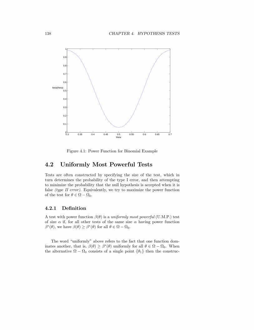
138 CHAPTER 4. HYPOTHESIS TESTS
0.3 0.35 0.4 0.45 0.5 0.55 0.6 0.65 0.70
0.1
0.2
0.3
0.4
0.5
0.6
0.7
0.8
0.9
1
theta
beta(theta)
Figure 4.1: Power Function for Binomial Example
4.2 Uniformly Most Powerful Tests
Tests are often constructed by specifying the size of the test, which inturn determines the probability of the type I error, and then attemptingto minimize the probability that the null hypothesis is accepted when it isfalse (type II error). Equivalently, we try to maximize the power functionof the test for θ ∈ Ω−Ω0.
4.2.1 Definition
A test with power function β(θ) is a uniformly most powerful (U.M.P.) testof size α if, for all other tests of the same size α having power functionβ∗(θ), we have β(θ) ≥ β∗(θ) for all θ ∈ Ω−Ω0.
The word “uniformly” above refers to the fact that one function dom-inates another, that is, β(θ) ≥ β∗(θ) uniformly for all θ ∈ Ω − Ω0. Whenthe alternative Ω − Ω0 consists of a single point θ1 then the construc-
4.2. UNIFORMLY MOST POWERFUL TESTS 139
tion of a best test is particularly easy. In this case, we may drop the word“uniformly” and refer to a “most powerful test”. The construction of abest test, by this definition, is possible under rather special circumstances.First, we often require a simple null hypothesis. This is the case when Ω0consists of a single point θ0 and so we are testing the null hypothesisH0 : θ = θ0.
4.2.2 Neyman-Pearson Lemma
LetX have probability (density) function f (x; θ) , θ ∈ Ω. Consider testing asimple null hypothesis H0 : θ = θ0 against a simple alternative H1 : θ = θ1.For a constant c, suppose the rejection region defined by
R = x; f (x; θ1)f (x; θ0)
> c
corresponds to a test of size α. Then the test with this rejection region isa most powerful test of size α for testing H0 : θ = θ0 against H1 : θ = θ1.
4.2.3 Proof
Consider another rejection region R1 with the same size. Then
P (X ∈ R; θ0) = P (X ∈ R1; θ0) = α or
ZR
f(x; θ0)dx =
ZR1
f(x; θ0)dx.
ThereforeZR∩R1
f(x; θ0)dx+
ZR∩R1
f(x; θ0)dx =
ZR∩R1
f(x; θ0)dx+
ZR∩R1
f(x; θ0)dx
and ZR∩R1
f(x; θ0)dx =
ZR∩R1
f(x; θ0)dx. (4.1)
For x ∈ R ∩ R1,
f(x; θ1)
f(x; θ0)> c or f(x; θ1) > cf(x; θ0)
and thus ZR∩R1
f(x; θ1) > c
ZR∩R1
f(x; θ0)dx. (4.2)
140 CHAPTER 4. HYPOTHESIS TESTS
For x ∈ R ∩R1, f(x; θ1) ≤ cf(x; θ0), and thus
−Z
R∩R1
f(x; θ1)dx ≥ −cZ
R∩R1
f(x; θ0)dx. (4.3)
Now
β(θ1) = P (X ∈ R; θ1) = P (X ∈ R ∩R1; θ1) + P (X ∈ R ∩ R1; θ1)
=
ZR∩R1
f(x; θ1)dx+
ZR∩R1
f(x; θ1)dx
and
β1(θ1) = P (X ∈ R1; θ1)
=
ZR∩R1
f(x; θ1)dx+
ZR∩R1
f(x; θ1)dx.
Therefore, using (4.1), (4.2), and (4.3) we have
β(θ1)− β1(θ1) =
ZR∩R1
f(x; θ1)dx−Z
R∩R1
f(x; θ1)dx
≥ c
ZR∩R1
f(x; θ0)dx− cZ
R∩R1
f(x; θ0)dx
= c
⎡⎢⎣ ZR∩R1
f(x; θ0)dx−Z
R∩R1
f(x; θ0)dx
⎤⎥⎦ = 0and the test with rejection region R is therefore the most powerful.¥
4.2.4 Example
Suppose X1, . . . ,Xn are independent N(θ, 1) random variables. We con-sider only the parameter space Ω = [0,∞). Suppose we wish to test thehypothesis H0 : θ = 0 against H1 : θ > 0.
(a) Choose an arbitrary θ1 > 0 and obtain the rejection region for the mostpowerful test of size 0.05 of H0 against H1 : θ = θ1.
(b) Does this test depend on the value of θ1 you chose? Can you concludethat it is uniformly most powerful?
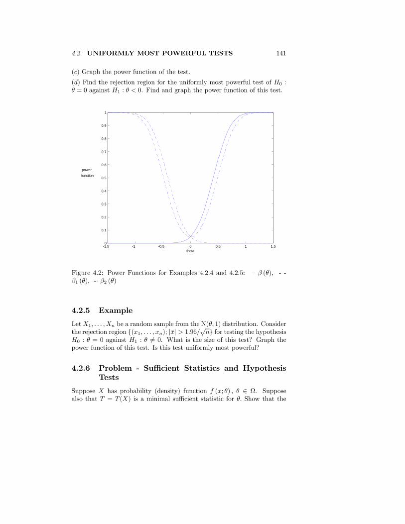
4.2. UNIFORMLY MOST POWERFUL TESTS 141
(c) Graph the power function of the test.
(d) Find the rejection region for the uniformly most powerful test of H0 :θ = 0 against H1 : θ < 0. Find and graph the power function of this test.
-1.5 -1 -0.5 0 0.5 1 1.50
0.1
0.2
0.3
0.4
0.5
0.6
0.7
0.8
0.9
1
theta
powerfunction
Figure 4.2: Power Functions for Examples 4.2.4 and 4.2.5: — β (θ), - -β1 (θ), -· β2 (θ)
4.2.5 Example
LetX1, . . . ,Xn be a random sample from the N(θ, 1) distribution. Considerthe rejection region (x1, . . . , xn); |x| > 1.96/
√n for testing the hypothesis
H0 : θ = 0 against H1 : θ 6= 0. What is the size of this test? Graph thepower function of this test. Is this test uniformly most powerful?
4.2.6 Problem - Sufficient Statistics and HypothesisTests
Suppose X has probability (density) function f (x; θ) , θ ∈ Ω. Supposealso that T = T (X) is a minimal sufficient statistic for θ. Show that the
142 CHAPTER 4. HYPOTHESIS TESTS
rejection region of the most powerful test of H0 : θ = θ0 against H1 : θ = θ1depends on the data X only through T.
4.2.7 Problem
Let X1, . . . ,X5 be a random sample from the distribution with probabilitydensity function
f (x; θ) =θ
xθ+1, x ≥ 1, θ > 0.
(a) Find the rejection region for the most powerful test of size 0.05 ofH0 : θ = 1 against H1 : θ = θ1 where θ1 > 1. Note: log (Xi) v EXP
¡1θ
¢.
(b) Explain why the rejection region in (a) is also the rejection region for theuniformly most powerful test of size 0.05 of H0 : θ = 1 against H1 : θ > 1.Sketch the power function of this test.
(c) Find the uniformly most powerful test of size 0.05 of H0 : θ = 1 againstH1 : θ < 1. On the same graph as in (b) sketch the power function of thistest.
(d) Explain why there is no uniformly most powerful test of H0 againstH1 : θ 6= 1. What reasonable test of size 0.05 might be used for testing H0against H1 : θ 6= 1? On the same graph as in (b) sketch the power functionof this test.
4.2.8 Problem
Let X1, . . . ,X10 be a random sample from the GAM(12 , θ) distribution.
(a) Find the rejection region for the most powerful test of size 0.05 ofH0 : θ = 2 against the alternative H1 : θ = θ1 where θ1 < 2.
(b) Explain why the rejection region in (a) is also the rejection region forthe uniformly most powerful test of size 0.05 of H0 : θ = 2 against thealternative H1 : θ < 2. Sketch the power function of this test.
(c) Find the uniformly most powerful test of size 0.05 of H0 : θ = 2 againstthe alternative H1 : θ > 2. On the same graph as in (b) sketch the powerfunction of this test.
(d) Explain why there is no uniformly most powerful test of H0 againstH1 : θ 6= 2. What reasonable test of size 0.05 might be used for testing H0against H1 : θ 6= 2? On the same graph as in (b) sketch the power functionof this test.
4.2. UNIFORMLY MOST POWERFUL TESTS 143
4.2.9 Problem
Let X1, . . . ,Xn be a random sample from the UNIF(0, θ) distribution. Findthe rejection region for the uniformly most powerful test of H0 : θ = 1against the alternative H1 : θ > 1 of size 0.01. Sketch the power functionof this test for n = 10.
4.2.10 Problem
We anticipate collecting observations (X1, . . . ,Xn) from a N(μ,σ2) distri-bution in order to test the hypothesis H0 : μ = 0 against the alternativeH1 : μ > 0 at level of significance 0.05. A preliminary investigation yieldsσ ≈ 2. How large a sample must we take in order to have power equal to0.95 when μ = 1?
4.2.11 Relationship Betweeen Hypothesis Tests andConfidence Intervals
There is a close relationship between hypothesis tests and confidence inter-vals as the following example illustrates. Suppose X1, . . . ,Xn is a randomsample from the N(θ, 1) distribution and we wish to test the hypothesis H0 :θ = θ0 against H1 : θ 6= θ0. The rejection region x; |x − θ0| > 1.96/
√n
is a size α = 0.05 rejection region which has a corresponding acceptanceregion x; |x−θ0| ≤ 1.96/
√n. Note that the hypothesis H0 : θ = θ0 would
not be rejected at the 0.05 level if |x− θ0| ≤ 1.96/√n or equivalently
x− 1.96/√n ≤ θ0 ≤ x+ 1.96/
√n
which is a 95% C.I. for θ.
4.2.12 Problem
Let (X1, . . . ,X5) be a random sample from the GAM(2, θ) distribution.Show that
R =
½x;
5Pi=1xi < 4.7955θ0 or
5Pi=1xi > 17.085θ0
¾is a size 0.05 rejection region for testing H0 : θ = θ0. Show how thisrejection region may be used to construct a 95% C.I. for θ.
144 CHAPTER 4. HYPOTHESIS TESTS
4.3 Locally Most Powerful Tests
It is not always possible to construct a uniformly most powerful test. Forthis reason, and because alternative values of the parameter close to thoseunder H0 are the hardest to differentiate from H0 itself, one may wish todevelop a test that is best able to test the hypthesis H0 : θ = θ0 againstalternatives very close to θ0. Such a test is called locally most powerful.
4.3.1 Definition
A test of H0 : θ = θ0 against H1 : θ > θ0 with power function β(θ) islocally most powerful if, for any other test having the same size and havingpower function β∗ (θ), there exists an ² > 0 such that β(θ) ≥ β∗ (θ) for allθ0 < θ < θ0 + ².
This definition asserts that there is a neighbourhood of the null hypoth-esis in which the test is most powerful.
4.3.2 Theorem
Suppose f (x; θ) ; θ ∈ Ω is a regular statistical model with correspondingscore function
S(θ;x) =∂
∂θlog f (x; θ) .
A locally most powerful test of H0 : θ = θ0 against H1 : θ > θ0 has rejectionregion
R = x; S(θ0;x) > c ,
where c is a constant determined by
P [S(θ0;X) > c; θ0] = size of test.
Since this test is based on the score function, it is also called a scoretest.
4.3.3 Example
Suppose X1, . . . ,Xn is a random sample from a N(θ, 1) distribution. Showthat the locally most powerful test of H0 : θ = 0 against H1 : θ > 0 is alsothe uniformly most powerful test.
4.3. LOCALLY MOST POWERFUL TESTS 145
4.3.4 Problem
Consider a single observation X from the LOG(1, θ) distribution. Find therejection region for the locally most powerful test of H0 : θ = 0 againstH1 : θ > 0. Is this test also uniformly most powerful? What is the powerfunction of the test?
SupposeX = (X1, . . . ,Xn) is a random sample from a regular statisticalmodel f (x; θ) ; θ ∈ Ω and the exact distribution of
S(θ0;X) =nPi=1
∂
∂θlog f(Xi; θ0)
is difficult to obtain. Since, under H0 : θ = θ0,
S(θ0;X)pJ (θ0)
→D Z v N(0, 1)
by the C.L.T., an approximate size α rejection region for testing H0 : θ = θ0against H1 : θ > θ0 is given by(
x;S(θ0;x)pJ (θ0)
≥ a)
where P (Z ≥ a) = α and Z v N(0, 1). J(θ0) may be replaced by I(θ0;x).
4.3.5 Example
Suppose X1, . . . ,Xn is a random sample from the CAU(1, θ) distribution.Find an approximate rejection region for a locally most powerful size 0.05test of H0 : θ = θ0 against H1 : θ < θ0. Hint: Show J(θ) = n/2.
4.3.6 Problem
Suppose X1, . . . ,Xn is a random sample from the WEI(1, θ) distribution.Find an approximate rejection region for a locally most powerful size 0.01test of H0 : θ = θ0 against H1 : θ > θ0.
Hint: Show that
J(θ) =n
θ2(1 +
π2
6+ γ2 − 2γ)
where
γ = −∞Z0
(log y)e−ydy ≈ 0.5772
is Euler’s constant.
146 CHAPTER 4. HYPOTHESIS TESTS
4.4 Likelihood Ratio Tests
Consider a test of the hypothesis H0 : θ ∈ Ω0 against H1 : θ ∈ Ω − Ω0.We have seen that for prescribed θ0 ∈ Ω0, θ1 ∈ Ω−Ω0, the most powerfultest of the simple null hypothesis H0 : θ = θ0 against a simple alternativeH1 : θ = θ1 is based on the likelihood ratio fθ1(x)/fθ0(x). By the Neyman-Pearson Lemma it has rejection region
R =
½x;f(x; θ1)
f(x; θ0)> c
¾where c is a constant determined by the size of the test. When either thenull or the alternative hypothesis are composite (i.e. contain more than onepoint) and there is no uniformly most powerful test, it seems reasonable touse a test with rejection region R for some choice of θ1, θ0. The likelihoodratio test does this with θ1 replaced by θ, the M.L. estimator over all possiblevalues of the parameter, and θ0 replaced by the M.L. estimator of theparameter when it is restricted to Ω0. Thus, the likelihood ratio test ofH0 : θ ∈ Ω0 versus H1 : θ ∈ Ω−Ω0 has rejection region R = x;Λ(x) > cwhere
Λ(x) =
supθ∈Ω
f (x; θ)
supθ∈Ω0
f (x; θ)=
supθ∈Ω
L (θ;x)
supθ∈Ω0
L (θ;x)
and c is determined by the size of the test. In general, the distribution ofthe test statistic Λ(X) may be difficult to find. Fortunately, however, theasymptotic distribution is known under fairly general conditions. In a fewcases, we can show that the likelihood ratio test is equivalent to the use ofa statistic with known distribution. However, in many cases, we need torely on the asymptotic chi-squared distribution of Theorem 4.4.7.
4.4.1 Example
Let X1, . . . ,Xn be a random sample from the N(μ,σ2) distribution whereμ and σ2 are unknown. Consider a test of
H0 : μ = 0, 0 < σ2 <∞
against the alternative
H1 : μ 6= 0, 0 < σ2 <∞.
(a) Show that the likelihood ratio test of H0 against H1 has rejection region
4.4. LIKELIHOOD RATIO TESTS 147
R = x;nx2/s2 > c.(b) Show under H0 that the statistic T = nX
2/S2 has a F(1, n− 1) distri-bution and thus find a size 0.05 test for n = 20.
(c) What rejection region would you use for testingH0 : μ = 0, 0 < σ2 <∞against the one-sided alternative H1 : μ > 0, 0 < σ2 <∞?
4.4.2 Problem
Suppose X ∼ GAM(2,β1) and Y ∼ GAM(2,β2) independently.(a) Show that the likelihood ratio statistic for testing the hypothesis H0 :β1 = β2 against the alternative H1 : β1 6= β2 is a function of the statisticT = X/(X + Y ).
(b) Find the distribution of T under H0.
(b) Find the rejection region for a size 0.01 test. What rejection regionwould you use for testing H0 : β1 = β2 against the one-sided alternativeH1 : β1 > β2?
4.4.3 Problem
Let (X1, . . . ,Xn) be a random sample from the N(μ,σ2) distribution andindependently let (Y1, . . . , Yn) be a random sample from the N(θ,σ2) dis-tribution where σ2 is known.
(a) Show that the likelihood ratio statistic for testing the hypothesis H0 :μ = θ against the alternative H1 : μ 6= θ is a function of T = |X − Y |.(b) Find the rejection region for a size 0.05 test. Is this test U.M.P.? Why?
4.4.4 Problem
Suppose X1, . . . ,Xn are independent EXP(λ) random variables and inde-pendently Y1, . . . , Ym are independent EXP(μ) random variables.
(a) Show that the likelihood ratio statistic for testing the hypothesis H0 :λ = μ against the alternative H1 : λ 6= μ is a function of
T =
nPi=1Xi∙
nPi=1Xi +
mPi=1Yi
¸ .
(b) Find the distribution of T under H0. Explain clearly how you wouldfind a size α = 0.05 rejection region.
148 CHAPTER 4. HYPOTHESIS TESTS
(c) For n = 20 find the rejection region for the one-sided alternative H1 :λ > μ for a size 0.05 test.
4.4.5 Problem
Suppose X1, . . . ,Xn is a random sample from the EXP(β,μ) distributionwhere β and μ are unknown.
(a) Show that the likelihood ratio statistic for testing the hypothesisH0 : β = 1 against the alternative H1 : β 6= 1 is a function of the statistic
T =nPi=1
¡Xi −X(1)
¢.
(b) Show that under H0, 2T has a chi-squared distribution (see Problem1.8.11).
(c) For n = 12 find the rejection region for the one-sided alternativeH1 : β > 1 for a size 0.05 test.
4.4.6 Problem
Let X1, . . . ,Xn be a random sample from the distribution with p.d.f.
f (x;α,β) =αxα−1
βα, 0 < x ≤ β.
(a) Show that the likelihood ratio statistic for testing the hypothesisH0 : α = 1 against the alternative H1 : α 6= 1 is a function of the statistic
T =nQi=1
¡Xi/X(n)
¢(b) Show that under H0, −2 log T has a chi-squared distribution (see Prob-lem 1.8.12).
(c) For n = 14 find the rejection region for the one-sided alternativeH1 : α > 1 for a size 0.05 test.
4.4.7 Problem
Suppose Yi ∼ N(α+βxi,σ2), i = 1, 2, . . . , n independently where x1, . . . , xnare known constants and α, β and σ2 are unknown parameters.
4.4. LIKELIHOOD RATIO TESTS 149
(a) Show that the likelihood ratio statistic for testing H0 : β = 0 againstthe alternative H1 : β 6= 0 is a function of
T =
β2nPi=1(xi − x)2
S2e
where
S2e =1
n− 2nPi=1(Yi − α− βxi)
2.
(b) What is the distribution of T under H0?
4.4.8 Theorem - Asymptotic Distribution of the Like-lihood Ratio Statistic (Regular Model)
Suppose X = (X1, . . . ,Xn) is a random sample from a regular statisticalmodel f (x; θ) ; θ ∈ Ω with Ω an open set in k−dimensional Euclideanspace. Consider a subset of Ω defined by Ω0 = θ(η); η ∈ open subset ofq-dimensional Euclidean space . Then the likelihood ratio statistic definedby
Λn(X)=
supθ∈Ω
nQi=1f (X; θ)
supθ∈Ω0
nQi=1f (X; θ)
=
supθ∈Ω
L (θ;X)
supθ∈Ω0
L (θ;X)
is such that, under the hypothesis H0 : θ ∈ Ω0,
2 logΛn(X)→D W v χ2(k − q).
Note: The number of degrees of freedom is the difference between thenumber of parameters that need to be estimated in the general model,and the number of parameters left to be estimated under the restrictionsimposed by H0.
4.4.9 Example
Suppose X1, . . . ,Xn are independent POI(λ) random variables and inde-pendently Y1, . . . , Yn are independent POI(μ) random variables.
(a) Find the likelihood ratio test statistic for testing H0 : λ = μ against thealternative H1 : λ 6= μ.
(b) Find the approximate rejection region for a size α = 0.05 test. Be sureto justify the approximation.
(c) Find the rejection region for the one-sided alternative H1 : λ < μ for asize 0.05 test.
150 CHAPTER 4. HYPOTHESIS TESTS
4.4.10 Problem
Suppose (X1,X2) ∼ MULT(n, θ1, θ2).(a) Find the likelihood ratio statistic for testing H0 : θ1 = θ2 = θ3 againstall alternatives.
(b) Find the approximate rejection region for a size 0.05 test. Be sure tojustify the approximation.
4.4.11 Problem
Suppose (X1,X2) ∼ MULT(n, θ1, θ2).(a) Find the likelihood ratio statistic for testing H0 : θ1 = θ2, θ2 = 2θ(1−θ)against all alternatives.
(a) Find the approximate rejection region for a size 0.05 test. Be sure tojustify the approximation.
4.4.12 Problem
Suppose (X1, Y1), . . . , (Xn, Yn) is a random sample from the BVN(μ,Σ)distribution with (μ,Σ) unknown.
(a) Find the likelihood ratio statistic for testing H0 : ρ = 0 against thealternative H1 : ρ 6= 0.(b) Find the approximate size 0.05 rejection region. Be sure to justify theapproximation.
4.4.13 Problem
Suppose in Problem 2.1.25 we wish to test the hypothesis that the dataarise from the assumed model. Show that the likelihood ratio statistic isgiven by
Λ = 2kPi=1
Fi log
µFiEi
¶where Ei = npi(θ) and θ is the M.L. estimator of θ.What is the asymptoticdistribution of Λ? Another test statistic which is commonly used is thePearson goodness of fit statistic given by
kPi=1
(Fi −Ei)2Ei
which also has an approximate χ2 distribution.
4.4. LIKELIHOOD RATIO TESTS 151
4.4.14 Problem
In Example 2.1.32 test the hypothesis that the data arise from the assumedmodel using the likelihood ratio statistic. Compare this with the answerthat you obtain using the Pearson goodness of fit statistic.
4.4.15 Problem
In Example 2.1.33 test the hypothesis that the data arise from the assumedmodel using the likelihood ratio statistic. Compare this with the answerthat you obtain using the Pearson goodness of fit statistic.
4.4.16 Problem
In Example 2.9.11 test the hypothesis that the data arise from the assumedmodel using the likelihood ratio statistic. Compare this with the answerthat you obtain using the Pearson goodness of fit statistic.
4.4.17 Problem
Suppose we have n independent repetitions of an experiment in which eachoutcome is classified according to whether event A occurred or not as wellas whether event B occurred or not. The observed data can be arrangedin a 2× 2 contingency table as follows:
B B TotalAA
f11 f12f21 f22
r1r2
Total c1 c2 n
Find the likelihood ratio statistic for testing the hypothesis that the eventsA and B are independent, that is, H0 : P (A ∩B) = P (A)P (B).
4.4.18 Problem
Suppose E(Y ) = Xβ where Y = (Y1, . . . , Yn)T is a vector of independent
and normally distributed random variables with V ar(Yi) = σ2, i = 1, . . . , n,X is a n × k matrix of known constants of rank k and β = (β1, . . . ,βk)
T
is a vector of unknown parameters. Find the likelihood ratio statistic fortesting the hypothesis H0 : βi = 0 against the alternative H1 : βi 6= 0 whereβi is the ith element of β.
152 CHAPTER 4. HYPOTHESIS TESTS
4.4.19 Signed Square-root Likelihood Ratio Statistic
Suppose X = (X1, . . . ,Xn) is a random sample from a regular statistical
model f (x; θ) ; θ ∈ Ω where θ = (θ1, θ2)T, θ1 is a scalar and Ω is an
open set in <k. Suppose also that the null hypothesis is H0 : θ1 = θ10.Let θ = (θ1, θ2) be the maximum likelihood of θ and let θ = (θ10, θ2 (θ10))where θ2 (θ10) is the maximum likelihood value of θ2 assuming θ1 = θ10.Then by Theorem 4.4.8
2 logΛn(X) = 2l(θ;X)− 2l(θ;X)→D W v χ2(1)
under H0 or equivalentlyh2l(θ;X)− 2l(θ;X)
i1/2→D Z v N(0, 1)
under H0. The signed square-root likelihood ratio statistic defined by
sign(θ1 − θ10)h2l(θ;X)− 2l(θ;X)
i1/2can be used to test one-sided alternatives such as H1 : θ1 > θ10 or H1 :θ1 < θ10. For example if the alternative hypothesis were H1 : θ1 > θ10 thenthe rejection region for an approximate size 0.05 test would be given by½
x; sign(θ1 − θ10)h2l(θ;X)− 2l(θ;X)
i1/2> 1.645
¾.
4.4.20 Problem - The Challenger Data
In Problem 2.8.9 test the hypothesis that β = 0. What would a sensiblealternative be? Describe in detail the null and the alternative hypothesesthat you have in mind and the relative costs of the two different kinds oferrors.
4.4.21 Significance Tests and p-values
We have seen that a test of hypothesis is a rule which allows us to decidewhether to accept the null hypothesis H0 or to reject it in favour of thealternative hypothesisH1 based on the observed data. A test of significancecan be used in situations in which H1 is difficult to specify. A (pure) testof significance is a procedure for measuring the strength of the evidenceprovided by the observed data against H0. This method usually involveslooking at the distribution of a test statistic or discrepancy measure Tunder H0. The p-value or significance level for the test is the probability,
4.5. SCORE AND MAXIMUM LIKELIHOOD TESTS 153
computed under H0, of observing a T value at least as extreme as the valueobserved. The smaller the observed p-value, the stronger the evidenceagainst H0. The difficulty with this approach is how to find a statisticwith ‘good properties’. The likelihood ratio statistic provides a general teststatistic which may be used.
4.5 Score and Maximum Likelihood Tests
4.5.1 Score or Rao Tests
In Section 4.3 we saw that the locally most powerful test was a score test.Score tests can be viewed as a more general class of tests of H0 : θ = θ0against H1 : θ ∈ Ω−θ0. If the usual regularity conditions hold then underH0 : θ = θ0 we have
S(θ0;X)[J(θ0)]−1/2 →D Z v N(0, 1).
and thus
R(X; θ0) = [S(θ0;X)]2[J(θ0)]−1 →D Y v χ2(1).
For a vector θ = (θ1, . . . , θk)T we have
R(X; θ0) = [S(θ0;X)]T [J(θ0)]−1S(θ0;X)→D Y v χ2(k). (4.4)
The corresponding rejection region is
R = x; R(x; θ0) > c
where c is determined by the size of the test, that is, c satisfiesP [R(X; θ0) > c; θ0] = α. An approximate value for c can be determinedusing P (Y > c) = α where Y v χ2(k).The test based onR(X; θ0) is asymptotically equivalent to the likelihood
ratio test. In (4.4) J(θ0) may be replaced by I(θ0) for an asymptoticallyequivalent test.Such test statistics are called score or Rao test statistics.
4.5.2 Maximum Likelihood or Wald Tests
Suppose that θ is the M.L. estimator of θ over all θ ∈ Ω and we wish to testH0 : θ = θ0 against H1 : θ ∈ Ω − θ0. If the usual regularity conditionshold then under H0 : θ = θ0
W (X; θ0) = (θ − θ0)TJ(θ0)(θ − θ0)→D Y v χ2(k). (4.5)
154 CHAPTER 4. HYPOTHESIS TESTS
The corresponding rejection region is
R = x; W (x; θ0) > c
where c is determined by the size of the test, that is, c satisfiesP [W (X; θ0) > c; θ0] = α. An approximate value for c can be determinedusing P (Y > c) = α where Y v χ2(k).
The test based on W (X; θ0) is asymptotically equivalent to the likeli-
hood ratio test. In (4.5) J(θ0) may also be replaced by J(θ), I(θ0) or I(θ)to obtain an asymptotically equivalent test statistic.
Such statistics are called maximum likelihood or Wald test statistics.
4.5.3 Example
Suppose X v POI (θ). Find the score test statistic (4.4) and the maximumlikelihood test statistic (4.5) for testing H0 : θ = θ0 against H1 : θ 6= θ0.
4.5.4 Problem
Find the score test statistic (4.4) and the Wald test statistic (4.5) for testingH0 : θ = θ0 against H1 : θ 6= θ0 based on a random sample (X1, . . . ,Xn)from each of the following distributions:
(a) EXP(θ)
(b) BIN(n, θ)
(c) N(θ,σ2), σ2 known
(d) EXP(θ,μ), μ known
(e) GAM(α, θ), α known
4.5.5 Problem
Let (X1, . . . ,Xn) be a random sample from the PAR(1, θ) distribution.Find the score test statistic (4.4) and the maximum likelihood test statistic(4.5) for testing H0 : θ = θ0 against H1 : θ 6= θ0.
4.5.6 Problem
Suppose (X1, . . . ,Xn) is a random sample from an exponential family modelf (x; θ) ; θ ∈ Ω. Show that the score test statistic (4.4) and the maximumlikelihood test statistic (4.5) for testing H0 : θ = θ0 against H1 : θ 6= θ0 areidentical if the maximum likelihood estimator of θ is a linear function ofthe natural sufficient statistic.
4.6. BAYESIAN HYPOTHESIS TESTS 155
4.6 Bayesian Hypothesis Tests
Suppose we have two simple hypotheses H0 : θ = θ0 and H1 : θ = θ1.The prior probability that H0 is true is denoted by P (H0) and the priorprobability that H1 is true is P (H1) = 1 − P (H0). P (H0)/P (H1) are theprior odds. Suppose also that the data x have probability (density) functionf (x; θ). The posterior probability thatHi is true is denoted by P (Hi|x), i =0, 1. The Bayesian aim in hypothesis testing is to determine the posteriorodds based on the data x given by
P (H0|x)P (H1|x)
=P (H0)
P (H1)× f(x; θ0)f(x; θ1)
.
The ratio f(x; θ0)/f(x; θ1) is called the Bayes factor. If P (H0) = P (H1)then the posterior odds are just a likelihood ratio. The Bayes factor mea-sures how the data have changed the odds as to which hypothesis is true.If the posterior odds were equal to q then a Bayesian would conclude thatH0 is q times more likely to be true than H1. A Bayesian may also decideto accept H0 rather than H1 if q is suitably large.If we have two composite hypotheses H0 : θ ∈ Ω0 and H1 : θ ∈ Ω− Ω0
then a prior distribution for θ must be specified for each hypothesis. Wedenote these by π0(θ|H0) and π1(θ|H1). In this case the posterior odds are
P (H0|x)P (H1|x)
=P (H0)
P (H1)·B
where B is the Bayes factor given by
B =
RΩ0
f (x; θ)π0(θ|H0)dθRΩ−Ω0
f (x; θ)π1(θ|H1)dθ.
For the hypotheses H0 : θ = θ0 and H1 : θ 6= θ0 the Bayes factor is
B =f(x; θ0)R
θ 6=θ0f (x; θ)π1(θ|H1)dθ
.
4.6.1 Problem
Suppose (X1, . . . ,Xn) is a random sample from a POI(θ) distribution andwe wish to test H0 : θ = θ0 against H1 : θ 6= θ0. Find the Bayes factor ifunder H1 the prior distribution for θ is the conjugate prior.

156 CHAPTER 4. HYPOTHESIS TESTS
Chapter 5
Appendix
5.1 Inequalities and Useful Results
5.1.1 Holder’s Inequality
Suppose X and Y are random variables and p and q are positive numberssatisfying
1
p+1
q= 1.
Then|E (XY )| ≤ E (|XY |) ≤ [E (|X|p)]1/p [E (|Y |q)]1/q .
Letting Y = 1 we have
E (|X|) ≤ [E (|X|p)]1/p , p > 1.
5.1.2 Covariance Inequality
If X and Y are random variables with variances σ21 and σ22 respectivelythen
[Cov (X,Y )]2 ≤ σ21σ22 .
5.1.3 Chebyshev’s Inequality
If X is a random variable with E(X) = μ and V ar(X) = σ2 <∞ then
P (|X − μ| ≥ k) ≤ σ2
k2.
for any k > 0.
157
158 CHAPTER 5. APPENDIX
5.1.4 Jensen’s Inequality
If X is a random variable and g (x) is a convex function then
E [g (X)] ≥ g [E (X)] .
5.1.5 Corollary
If X is a non-degenerate random variable and g (x) is a strictly convexfunction. Then
E [g (X)] > g [E (X)] .
5.1.6 Stirling’s Formula
For large nΓ (n+ 1) ≈
√2πnn+1/2e−n.
5.1.7 Matrix Differentiation
Suppose x = (x1, . . . , xk)T, b = (b1, . . . , bk)
Tand A is a k × k symmetric
matrix. Then
∂
∂x
¡xT b
¢=
∙∂
∂x1
¡xT b
¢, . . . ,
∂
∂xk
¡xT b
¢¸T= b
and∂
∂x
¡xTAx
¢=
∙∂
∂x1
¡xTAx
¢, . . . ,
∂
∂xk
¡xTAx
¢¸T= 2Ax.
5.2. DISTRIBUTIONAL RESULTS 159
5.2 Distributional Results
5.2.1 Functions of Random Variables
Univariate One-to-One Transformation
Suppose X is a continuous random variable with p.d.f. f (x) and supportset A. Let Y = h (X) be a real-valued, one-to-one function from A to B.Then the probability density function of Y is
g (y) = f¡h−1 (y)
¢·¯d
dyh−1 (y)
¯, y ∈ B.
Multivariate One-to-One Transformation
Suppose (X1, . . . ,Xn) is a vector of random variables with joint p.d.f.f (x1, . . . , xn) and support set RX . Suppose the transformation S definedby
Ui = hi(X1, . . . ,Xn), i = 1, . . . , n
is a one-to-one, real-valued transformation with inverse transformation
Xi = wi(U1, . . . , Un), i = 1, . . . , n.
Suppose also that S maps RX into RU . Then g(u1, . . . , un), the joint p.d.f.of (U1, . . . , Un) , is given by
g(u) = f(w1(u), . . . , wn(u))
¯∂(x1, . . . , xn)
∂(u1, . . . , un)
¯, (u1, . . . , un) ∈ RU
where
∂(x1, . . . , xn)
∂(u1, . . . , un)=
¯¯
∂x1∂u1
· · · ∂x1∂un
......
∂xn∂u1
· · · ∂xn∂un
¯¯ = ∙∂(u1, . . . , un)
∂(x1, . . . , xn)
¸−1
is the Jacobian of the transformation.
160 CHAPTER 5. APPENDIX
5.2.2 Order Statistic
The following results are derived in Casella and Berger, Section 5.4.
Joint Distribution of the Order Statistic
SupposeX1, . . . ,Xn is a random sample from a continuous distribution withprobability density function f (x). The joint probability density functionof the order statistic T =
¡X(1), . . . ,X(n)
¢= (T1, . . . , Tn) is
g (t1, . . . , tn) = n!nQi=1f (ti) , −∞ < t1 < · · · < tn <∞.
Distribution of the Maximum and the Minimum of a Vector ofRandom Variables
Suppose X1, . . . ,Xn is a random sample from a continuous distributionwith probability density function f (x), support set A, and cumulative dis-tribution function F (x).
The probability density function of U = X(i), i = 1, . . . , n is
n!
(i− 1)! (n− i)!f (u) [F (u)]i−1
[1− F (u)]n−i , u ∈ A.
In particular the probability density function of T = X(n) = max (X1, ...,Xn)is
g1 (t) = nf (t) [F (t)]n−1 , t ∈ A
and the probability density function of S = X(1) = min (X1, ...,Xn) is
g2 (s) = nf (s) [1− F (s)]n−1 , s ∈ A.
5.2. DISTRIBUTIONAL RESULTS 161
The joint p.d.f. of U = X(i) and V = X(j), 1 ≤ i < j ≤ n is given by
n!
(i− 1)! (j − 1− i)! (n− j)!f (u) f (v) [F (u)]i−1
[F (v)− F (u)] [1− F (v)]n−j ,
u < v, u ∈ A, v ∈ A.
In particular the joint probability density function of S = X(1) andT = X(n) is
g (s, t) = n (n− 1) f (s) f (t) [F (t)− F (s)]n−2 , s < t, s ∈ A, t ∈ A.
5.2.3 Problem
If Xi ∼ UNIF(a, b), i = 1, . . . , n independently, then show
X(1) − ab− a ∼ BETA(1, n)
X(n) − ab− a ∼ BETA(n, 1)
162 CHAPTER 5. APPENDIX
5.2.4 Distribution of Sums of Random Variables
(1) If Xi ∼ POI(μi), i = 1, . . . , n independently, thennPi=1Xi ∼ POI
µnPi=1
μi
¶.
(2) If Xi ∼ BIN(ni, p), i = 1, . . . , n independently, thennPi=1Xi ∼ BIN
µnPi=1ni, p
¶.
(3) If Xi ∼ NB(ki, p), i = 1, . . . , n independently, thennPi=1Xi ∼ NB
µnPi=1ki, p
¶.
(4) If Xi ∼ N(μi,σ2i ), i = 1, . . . , n independently, thennPi=1aiXi ∼ N
µnPi=1aiμi,
nPi=1a2iσ
2i
¶.
(5) If Xi ∼ N(μ,σ2), i = 1, . . . , n independently, thennPi=1
Xi ∼ N¡nμ, nσ2
¢and X ∼ N
¡μ, σ2/n
¢.
(6) If Xi ∼ GAM(αi,β), i = 1, . . . , n independently, thennPi=1Xi ∼ GAM
µnPi=1
αi, β
¶.
(7) If Xi ∼ GAM(1,β) = EXP(β), i = 1, . . . , n independently, thennPi=1Xi ∼ GAM(n, β) .
(8) If Xi ∼ χ2 (ki), i = 1, . . . , n independently, then
nPi=1Xi ∼ χ2
µnPi=1ki
¶.
(9) If Xi ∼ GAM(αi,β), i = 1, . . . , n independently where αi is a posi-tive integer, then
2
β
nPi=1Xi ∼ χ2
µ2
nPi=1
αi
¶.
(10) If Xi ∼ N(μ,σ2), i = 1, . . . , n independently, thennPi=1
µXi − μ
σ
¶2∼ χ2 (n) .
5.2. DISTRIBUTIONAL RESULTS 163
5.2.5 Theorem - Properties of the Multinomial Distri-bution
Suppose (X1, . . . ,Xk) ∼MULT(n, p1, . . . , pk) with joint p.f.
f(x1, . . . , xk) =n!
x1!x2! · · ·xk+1!px11 p
x22 · · · p
xk+1k+1
xi = 0, . . . , n, i = 1, . . . , k+1, xk+1 = n−kPi=1xi, 0 < pi < 1, i = 1, . . . , k+1,
k+1Pi=1
pi = 1. Then
(1) (X1, . . . ,Xk) has joint m.g.f.
M(t1, . . . , tk) = (p1et1 + · · ·+ pketk + pk+1)n, (t1, . . . , tk) ∈ <k.
(2) Any subset of X1, . . . ,Xk+1 also has a multinomial distribution. Inparticular
Xi v BIN (n, pi) , i = 1, . . . , k + 1.
(3) If T = Xi +Xj , i 6= j, then
T v BIN (n, pi + pj) .
(4)
Cov (Xi,Xj) = −nθiθj .
(5) The conditional distribution of any subset of (X1, . . . ,Xk+1) given therest of the coordinates is a multinomial distribution. In particular theconditional p.f. of Xi given Xj = xj , i 6= j, is
Xi|Xj = xj ∼ BINµn− xj ,
pi1− pj
¶.
(6) The conditional distribution of Xi given T = Xi +Xj = t, i 6= j, is
Xi|Xi +Xj = t ∼ BINµt,
pipi + pj
¶.
164 CHAPTER 5. APPENDIX
5.2.6 Definition - Multivariate Normal Distribution
Let X = (X1, . . . ,Xk)T be a k × 1 random vector with E(Xi) = μi and
Cov(Xi,Xj) = σij , i, j = 1, . . . , k. (Note: Cov(Xi,Xi) = σii = V ar(Xi) =σ2i .) Let μ = (μ1, . . . ,μk)
T be the mean vector and Σ be the k×k symmetriccovariance matrix whose (i, j) entry is σij . Suppose also that Σ
−1 exists. Ifthe joint p.d.f. of (X1, . . . ,Xk) is given by
f(x1, . . . , xk) =1
(2π)k/2|Σ|1/2 exp∙−12(x− μ)TΣ−1(x− μ)
¸, x ∈ Rk
where x = (x1, . . . , xk)T then X is said to have a multivariate normal
distribution. We write X v MVN(μ,Σ).
5.2.7 Theorem - Properties of the MVN Distribution
Suppose X = (X1, . . . ,Xk)T v MVN(μ,Σ). Then
(1) X has joint m.g.f.
M(t) = exp
µμT t+
1
2tTΣt
¶, t = (t1, . . . , tk)
T ∈ <k.
(2) Any subset of X1, . . . ,Xk also has a MVN distribution and in particular
Xi v N(μi, σ2i ), i = 1, . . . , k.(3)
(X − μ)TΣ−1(X − μ) v χ2(k).
(4) Let c = (c1, . . . , ck)T be a nonzero vector of constants then
cTX =kPi=1ciXi v N(cTμ, cTΣc).
(5) Let A be a k × p vector of constants of rank p then
ATX v N(ATμ, ATΣA).
(6) The conditional distribution of any subset of (X1, . . . ,Xk) given the
rest of the coordinates is a multivariate normal distribution. In particularthe conditional p.d.f. of Xi given Xj = xj , i 6= j, is
Xi|Xj = xj ∼ N(μi + ρijσi(xj − μj)/σj , (1− ρ2ij)σ2i )
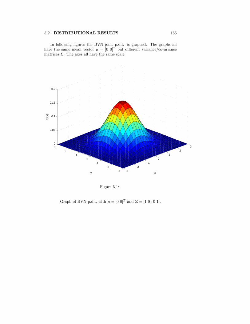
5.2. DISTRIBUTIONAL RESULTS 165
In following figures the BVN joint p.d.f. is graphed. The graphs allhave the same mean vector μ = [0 0]T but different variance/covariancematrices Σ. The axes all have the same scale.
-3-2
-10
12
3
-3-2
-10
12
30
0.05
0.1
0.15
0.2
xy
f(x,y
)
Figure 5.1:
Graph of BVN p.d.f. with μ = [0 0]T and Σ = [1 0 ; 0 1].
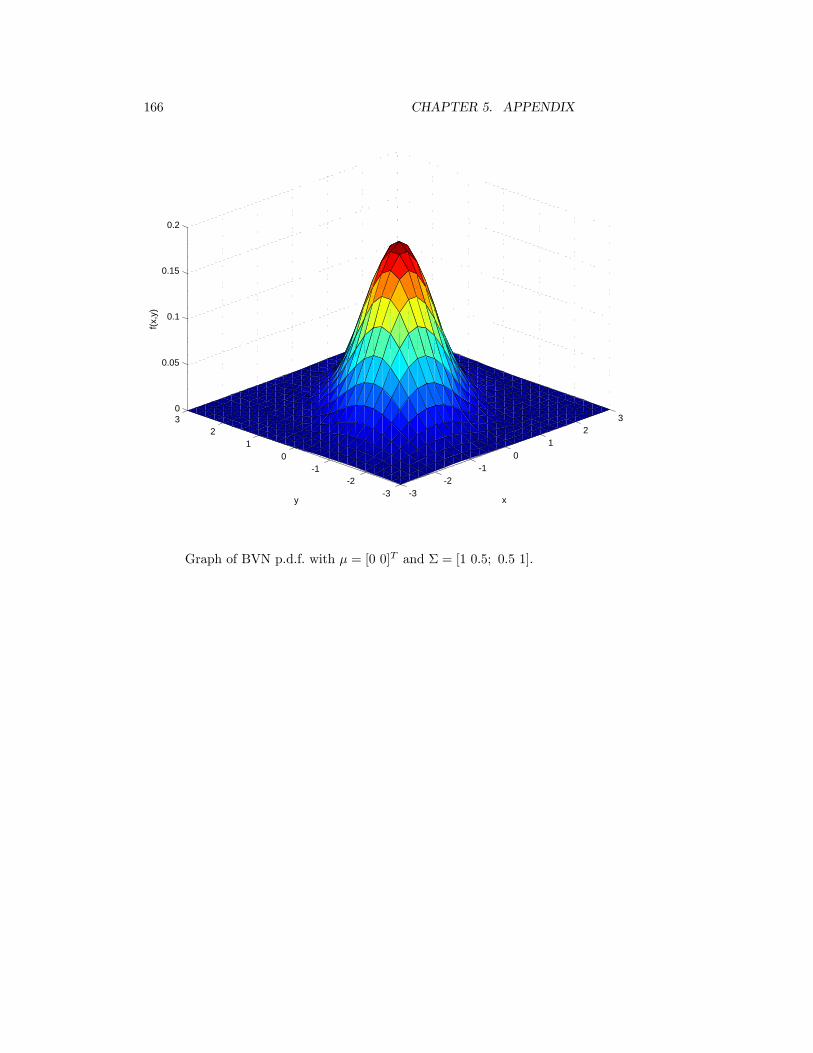
166 CHAPTER 5. APPENDIX
-3-2
-10
12
3
-3-2
-10
12
30
0.05
0.1
0.15
0.2
xy
f(x,y
)
Graph of BVN p.d.f. with μ = [0 0]T and Σ = [1 0.5; 0.5 1].
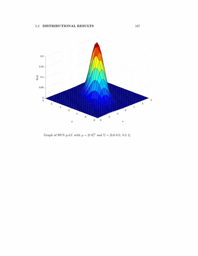
5.2. DISTRIBUTIONAL RESULTS 167
-3-2
-10
12
3
-3-2
-10
12
30
0.05
0.1
0.15
0.2
xy
f(x,y
)
Graph of BVN p.d.f. with μ = [0 0]T and Σ = [0.6 0.5; 0.5 1].
168 CHAPTER 5. APPENDIX
5.3 Limiting Distributions
5.3.1 Definition - Convergence in Probability to a Con-stant
The sequence of random variables X1,X2, . . . ,Xn, . . . converges in proba-bility to the constant c if for each ² > 0
limn→∞
P (|Xn − c| ≥ ²) = 0.
We write Xn →p c.
5.3.2 Theorem
If X1,X2, ...,Xn, ... is a sequence of random variables such that
limn→∞
P (Xn ≤ x) =½0 x < b
1 x > b
then Xn →p b.
5.3.3 Theorem - Weak Law of Large Numbers
If X1, . . . ,Xn is a random sample from a distribution withE(Xi) = μ and V ar(Xi) = σ2 <∞ then
Xn =1
n
nPi=1Xi →p μ.
5.3.4 Problem
Suppose X1,X2, . . . ,Xn, . . . is a sequence of random variables such thatE(Xn) = c and lim
n→∞V ar(Xn) = 0. Show that Xn →p c.
5.3.5 Problem
Suppose X1,X2, . . . ,Xn, . . . is a sequence of random variables such thatXn/n→p b < 0. Show that lim
n→∞P (Xn < 0) = 1.
5.3.6 Problem
Show that if Yn →p a and
limn→∞
P (|Xn| ≤ Yn) = 1
5.3. LIMITING DISTRIBUTIONS 169
then Xn is bounded in probability, that is, there exists b > 0 such that
limn→∞
P (|Xn| ≤ b) = 1.
5.3.7 Definition - Convergence in Distribution
The sequence of random variables X1,X2, . . . ,Xn, . . . converges in distrib-ution to a random variable X if
limn→∞
P (Xn ≤ x) = P (X ≤ x) = F (x)
for all values of x at which F (x) is continuous. We write Xn →D X.
5.3.8 Theorem
Suppose X1, ...,Xn, ... is a sequence of random variables with E(Xn) = μnand V ar(Xn) = σ2n. If lim
n→∞μn = μ and lim
n→∞σ2n = 0 then Xn →p μ.
5.3.9 Central Limit Theorem
If X1, . . . ,Xn is a random sample from a distribution withE(Xi) = μ and V ar(Xi) = σ2 <∞ then
Yn =
nPi=1Xi − nμ√nσ
=
√n(Xn − μ)
σ→D Z v N(0, 1).
5.3.10 Limit Theorems
1. If Xn →p a and g is continuous at a, then g(Xn)→p g(a).
2. If Xn →p a, Yn →p b and g(x, y) is continuous at (a, b) theng(Xn, Yn)→p g(a, b).
3. (Slutsky) If Xn →D X, Yn →p b and g(x, b) is continuous for allx ∈ support of X then g(Xn, Yn)→D g(X, b).
4. (Delta Method) If X1,X2, ...,Xn, ... is a sequence of random variablessuch that
nb(Xn − a)→D X
for some b > 0 and if the function g(x) is differentiable at a withg0(a) 6= 0 then
nb[g(Xn)− g(a)]→D g0(a)X.

170 CHAPTER 5. APPENDIX
5.3.11 Problem
If Xn →p a > 0, Yn →p b 6= 0 and Zn →D Z ∼ N(0, 1) then find thelimiting distributions of
(1) X2n (2)
pXn (3) XnYn (4) Xn + Yn (5) Xn/Yn
(6) 2Zn (7) Zn + Yn (8) XnZn (9) Z2n (10) 1/Zn
5.4. PROOFS 171
5.4 Proofs
5.4.1 Theorem
Suppose the model is f (x; θ) ; θ ∈ Ω and let A = support of X. PartitionA into the equivalence classes defined by
Ay =½x;f (x; θ)
f(y; θ)= H(x, y) for all θ ∈ Ω
¾, y ∈ A. (5.1)
This is a minimal sufficient partition. The statistic T (X) which inducesthis partition is a minimal sufficient statistic.
5.4.2 Proof
We give the proof for the case in which A does not depend on θ.Let T (X) be the statistic which induces the partition in (5.1). To show
that T (X) is sufficient we define
B = t : t = T (x) for some x ∈ A .
Then the set A can be written as
A = ∪t∈BAt
where
At = x : T (x) = t , t ∈ B.
The statistic T (X) induces the partition defined by At, t ∈ B. For eachAt we can choose and fix one element, xt ∈ A. Obviously T (xt) = t. Letg (t; θ) be a function defined on B such that
g (t; θ) = f (xt; θ) , t ∈ B.
Consider any x ∈ A. For this x we can calculate T (x) = t and thusdetermine the set At to which x belongs as well as the value xt which waschosen for this set. Obviously T (x) = T (xt). By the definition of thepartition induced by T (X), we know that for all x ∈ At, f (x; θ) /f (xt; θ) isa constant function of θ. Therefore for any x ∈ A we can define a function
h (x) =f (x; θ)
f (xt; θ)
where T (x) = T (xt) = t.
172 CHAPTER 5. APPENDIX
Therefore for all x ∈ A and θ ∈ Ω we have
f (x; θ) = f (xt; θ)f (x; θ)
f (xt; θ)
= g (t; θ)h (x)
= g (T (xt) ; θ)h (x)
= g (T (x) ; θ)h (x)
and by the Factorization Criterion for Sufficieny T (X) is a sufficient sta-tistic.To show that T (X) is a minimal sufficient statistic suppose that T1 (X)
is any other sufficient statistic. By the Factorization Criterion for Sufficieny,there exist functions h1 (x) and g1 (t; θ) such that
f (x; θ) = g1 (T1 (x) ; θ)h1 (x)
for all x ∈ A and θ ∈ Ω. Let x and y be any two points in A withT1 (x) = T1 (y). Then
f (x; θ)
f (y; θ)=
g1 (T1 (x) ; θ)h1 (x)
g1 (T1 (y) ; θ)h1 (y)
=h1 (x)
h1 (y)
= function of x and y which does not depend on θ
and therefore by the definition of T (X) this implies T (x) = T (y). Thisimplies that T1 induces either the same partition of A as T (X) or it inducesa finer partition of A than T (X) and therefore T (X) is a function of T1 (X).Since T (X) is a function of every other sufficient statistic, therefore T (X)is a minimal sufficient statistic.
5.4.3 Theorem
If T (X) is a complete sufficient statistic for the model f (x; θ) ; θ ∈ Ωthen T (X) is a minimal sufficient statistic for f (x; θ) ; θ ∈ Ω.
5.4.4 Proof
Suppose U = U (X) is a minimal sufficient statistic for the modelf (x; θ) ; θ ∈ Ω. The function E (T |U) is a function of U which does notdepend on θ since U is a sufficient statistic. Also by Definition 1.5.2, U is
5.4. PROOFS 173
a function of the sufficient statistic T which implies E (T |U) is a functionof T .Let
h (T ) = T −E (T |U) .
Now
E [h (T ) ; θ] = E [T − E (T |U) ; θ]= E (T ; θ)−E [E (T |U) ; θ]= E (T ; θ)−E (T ; θ)= 0, for all θ ∈ Ω.
Since T is complete this implies
P [h (T ) = 0; θ] = 1, for all θ ∈ Ω
or
P [T = E (T |U)] = 1, for all θ ∈ Ω
and therefore T is a function of U . This can only be true if T is also aminimal sufficent statistic for the model.
The regularity conditions are repeated here since they are used in theproofs that follow.
5.4.5 Regularity Conditions
Consider the model f (x; θ) ; θ ∈ Ω. Suppose that:
(R1) The parameter space Ω is an open interval in the real line.
(R2) The densities f (x; θ) have common support, so that the setA = x; f (x; θ) > 0 , does not depend on θ.
(R3) For all x ∈ A, f (x; θ) is a continuous, three times differentiable func-tion of θ.
(R4) The integralRA
f (x; θ) dx can be twice differentiated with respect to θ
under the integral sign, that is,
∂k
∂θk
ZA
f (x; θ) dx =
ZA
∂k
∂θkf (x; θ) dx, k = 1, 2 for all θ ∈ Ω.
174 CHAPTER 5. APPENDIX
(R5) For each θ0 ∈ Ω there exist a positive number c and function M (x)(both of which may depend on θ0), such that for all θ ∈ (θ0 − c, θ0 + c)¯
∂3 log f (x; θ)
∂θ3
¯< M(x)
holds for all x ∈ A, and
E [M (X) ; θ] <∞ for all θ ∈ (θ0 − c, θ0 + c) .
(R6) For each θ ∈ Ω,
0 < E
(∙∂2 log f (X; θ)
∂θ2
¸2; θ
)<∞
(R7) The probability (density) functions corresponding to different values
of the parameters are distinct, that is, θ 6= θ∗ =⇒ f (x; θ) 6= f (x; θ∗).
The following lemma is required for the proof of consistency of the M.L.estimator.
5.4.6 Lemma
If X is a non-degenerate random variable with model f (x; θ) ; θ ∈ Ω sat-isfying (R1)− (R7) then
E [log f (X; θ)− log f (X; θ0) ; θ0] < 0 for all θ, θ0 ∈ Ω, and θ 6= θ0.
5.4.7 Proof
Since g (x) = − log x is strictly convex and X is a non-degenerate randomvariable then by the corollary to Jensen’s inequality
E [log f (X; θ)− log f (X; θ0) ; θ0] = E
½log
∙f (X; θ)
f (X; θ0)
¸; θ0
¾< log
½E
∙f (X; θ)
f (X; θ0); θ0
¸¾for all θ, θ0 ∈ Ω, and θ 6= θ0.
5.4. PROOFS 175
Since
E
∙f (X; θ)
f (X; θ0); θ0
¸=
ZA
f (x; θ)
f (x; θ0)f (x; θ0) dx
=
ZA
f (x; θ) dx = 1, for all θ ∈ Ω
therefore
E [l (θ;X)− l (θ0;X) ; θ0] < log (1) = 0, for all θ, θ0 ∈ Ω, and θ 6= θ0.
5.4.8 Theorem
Suppose (X1, . . . ,Xn) is a random sample from a model f (x; θ) ; θ ∈ Ωsatisfying regularity conditions (R1)−(R7). Then with probability tendingto 1 as n→∞, the likelihood equation or score equation
nXi=1
∂
∂θlogf (Xi; θ) = 0
has a root θn such that θn converges in probability to θ0, the true value ofthe parameter, as n→∞.
5.4.9 Proof
Let
ln (θ;X) = ln (θ;X1, . . . ,Xn)
= log
∙nQi=1f (Xi; θ)
¸=
nPi=1logf (Xi; θ) , θ ∈ Ω.
Since f (x; θ) is differentiable with respect to θ for all θ ∈ Ω this impliesln (θ;x) is differentiable with respect to θ for all θ ∈ Ω and also ln (θ;x) isa continuous function of θ for all θ ∈ Ω.By the above lemma we have for any δ > 0 such that θ0 ± δ ∈ Ω,
E [ln (θ0 + δ;X)− ln (θ0;X) ; θ0] < 0 (5.2)
andE [ln (θ0 − δ;X)− ln (θ0;X) ; θ0] < 0. (5.3)
176 CHAPTER 5. APPENDIX
By (5.2) and the WLLN
1
n[ln (θ;X)− ln (θ0;X)]→p b < 0
which implies
limn→∞
P [ln (θ0 + δ;X)− ln (θ0;X) < 0] = 1
(see Problem 5.3.5). Therefore there exists a sequence of constants ansuch that 0 < an < 1, lim
n→∞an = 0 and
P [ln (θ0 + δ;X)− ln (θ0;X) < 0] = 1− an.
Let
An = An (δ) = x : ln (θ0 + δ;x)− ln (θ0;x) < 0
where x = (x1, . . . , xn). Then
limn→∞
P (An; θ0) = limn→∞
(1− an) = 1.
Let
Bn = Bn (δ) = x : ln (θ0 − δ;x)− ln (θ0;x) < 0 .
then by the same argument as above there exists a sequence of constantsbn such that 0 < bn < 1, lim
n→∞bn = 0 and
limn→∞
P (Bn; θ0) = limn→∞
(1− bn) = 1.
Now
P (An ∩Bn; θ0) = P (An; θ0) + P (Bn; θ0)− P (An ∪Bn; θ0)= 1− an + 1− bn − P (An ∪Bn; θ0)= 1− an − bn + [1− P (An ∪Bn; θ0)]≥ 1− an − bn
since 1− P (An ∪Bn; θ0) ≥ 0. Therefore
limn→∞
P (An ∩Bn; θ0) = limn→∞
(1− an − bn) = 1 (5.4)
Continuity of ln (θ;x) for all θ ∈ Ω implies that for any x ∈ An ∩ Bn,there exists a value θn (δ) = θn (δ;x) ∈ (θ0 − δ, θ0 + δ) such that ln (θ;x)
5.4. PROOFS 177
has a local maximum at θ = θn (δ). Since ln (θ;x) is differentiable withrespect to θ this implies (Fermat’s theorem)
∂ln (θ;x)
∂θ=
nXi=1
∂
∂θlogf (xi; θ) = 0 for θ = θn (δ) .
Note that ln (θ;x) may have more than one local maximum on the interval
(θ0 − δ, θ0 + δ) and therefore θn (δ) may not be unique. If x /∈ An ∩ Bn,then θn (δ) may not exist in which case we define θn (δ) to be a fixed ar-
bitrary value. Note also that the sequence of rootsnθn (δ)
odepends on
δ.Let θn = θn (x) be the value of θ closest to θ0 such that
∂ln (θ;x) /∂θ = 0. If such a root does not exist we define θn to be a fixedarbitrary value. Since
1 ≥ Phθn ∈ (θ0 − δ, θ0 + δ) ; θ0
i≥ P
hθn (δ) ∈ (θ0 − δ, θ0 + δ) ; θ0
i≥ P (An ∩Bn; θ0) (5.5)
then by (5.4) and the Squeeze Theorem we have
limn→∞
Phθn ∈ (θ0 − δ, θ0 + δ) ; θ0
i= 1.
Since this is true for all δ > 0, θn →p θ0.
5.4.10 Theorem
Suppose (R1)− (R7) hold. Suppose θn is a consistent root of the likelihoodequation as in Theorem 5.4.8. Thenp
J(θ0)(θn − θ0)→D Z ∼ N(0, 1)
where θ0 is the true value of the parameter.
5.4.11 Proof
Let
S1 (θ;x) =∂
∂θlog f (x; θ)
and
I1 (θ;x) = −∂
∂θS1 (θ;x) = −
∂2
∂θ2log f (x; θ)
178 CHAPTER 5. APPENDIX
be the score and information functions respectively for one observation fromf (x; θ) ; θ ∈ Ω. Since f (x; θ) ; θ ∈ Ω is a regular model
E [S1 (θ;X) ; θ] = 0, θ ∈ Ω (5.6)
and
V ar [S1 (θ;X)] ; θ = E [I1 (θ;x) ; θ] = J1 (θ) <∞, θ ∈ Ω. (5.7)
Let
An =
½(x1, . . . , xn) ; such that
nPi=1
∂
∂θlogf (xi; θ) =
nPi=1S1 (θ;xi) = 0 has a solution
¾and for (x1, . . . , xn) ∈ An, let θn = θn (x1, . . . , xn) be the value of θ such
thatnPi=1S1(θn;xi) = 0.
ExpandnPi=1S1(θn;xi) as a function of θn about θ0 to obtain
nPi=1S1(θn;xi) =
nPi=1S1 (θ0;xi)− (θn − θ0)
nPi=1I1 (θ;xi)
+1
2(θn − θ0)
2nPi=1
∂3
∂θ3log f (xi; θ) |θ=θ∗n (5.8)
where θ∗n = θ∗n (x1, . . . , xn) lies between θ0 and θn by Taylor’s Theorem.Suppose (x1, . . . , xn) ∈ An. Then the left side of (5.8) equals zero and
thus
nPi=1S1 (θ0;xi) = (θn − θ0)
nPi=1I1 (θ;xi)−
1
2(θn − θ0)
2nPi=1
∂3
∂θ3log f (xi; θ) |θ=θ∗n
= (θn − θ0)
∙nPi=1I1 (θ;xi)−
1
2(θn − θ0)
2nPi=1
∂3
∂θ3log f (xi; θ) |θ=θ∗n
¸or
nPi=1S1 (θ0;xi)pnJ1 (θ0)
=(θn − θ0)pnJ1 (θ0)
∙nPi=1I1 (θ;xi)−
1
2(θn − θ0)
2nPi=1
∂3
∂θ3log f (xi; θ) |θ=θ∗n
¸
=pJ (θ0)(θn − θ0)
⎡⎢⎢⎣1n
nPi=1I1 (θ;xi)
J1 (θ0)− 12(θn − θ0)
2
1n
nPi=1
∂3
∂θ3 log f (xi; θ) |θ=θ∗nJ1 (θ0)
⎤⎥⎥⎦
5.4. PROOFS 179
Therefore for (X1, . . . ,Xn) we have⎡⎢⎢⎣nPi=1S1 (θ0;Xi)pnJ1 (θ0)
⎤⎥⎥⎦ I(X1, . . . ,Xn) ∈ An (5.9)
=pJ (θ0)(θn−θ0)
⎡⎢⎢⎣1n
nPi=1I1 (θ;Xi)
J1 (θ0)− (θn − θ0)
2
2J1 (θ0)
nPi=1
∂3
∂θ3 log f (Xi; θ) |θ=θ∗nn
⎤⎥⎥⎦ I(X1, . . . ,Xn) ∈ Anwhere θ∗n = θ∗n (X1, . . . ,Xn) . By an argument similar to that used in Proof5.4.4
limn→∞
P [(X1, . . . ,Xn) ∈ An; θ0] = 1. (5.10)
Since S1 (θ0;Xi), i = 1, . . . , n are i.i.d. random variables with mean andvariance given by (5.6) and (5.7) then by the CLT
nPi=1S1 (θ0;Xi)pnJ1 (θ0)
→D Z v N(0, 1) . (5.11)
Since I1 (θ0;Xi), i = 1, . . . , n are i.i.d. random variables with meanJ1 (θ) then by the WLLN
1
n
nPi=1I1 (θ;Xi)→p J1 (θ)
and thus1n
nPi=1I1 (θ;Xi)
J1 (θ0)→p 1 (5.12)
by the Limit Theorems.To complete the proof we need to show
(θn − θ0)2
∙1
n
nPi=1
∂3
∂θ3log f (Xi; θ) |θ=θ∗n
¸→p 0. (5.13)
Since θn →p θ0 we only need to show that
1
n
nPi=1
∂3
∂θ3log f (Xi; θ) |θ=θ∗n (5.14)
180 CHAPTER 5. APPENDIX
is bounded in probability. Since θn →p θ0 implies θ∗n →p θ0 then by (R5)
limn→∞
P
½¯1
n
nPi=1
∂3
∂θ3log f (Xi; θ) |θ=θ∗n
¯≤ 1
n
nPi=1M (Xi) ; θ0
¾= 1.
Also by (R5) and the WLLN
1
n
nPi=1M (Xi)→p E[M(X); θ0] <∞.
It follows that (5.14) is bounded in probability (see Problem 5.3.6).Therefore p
J (θ0)(θn − θ0)→D Z v N(0, 1)follows from (5.9), (5.11)-(5.13) and Slutsky’s Theorem.
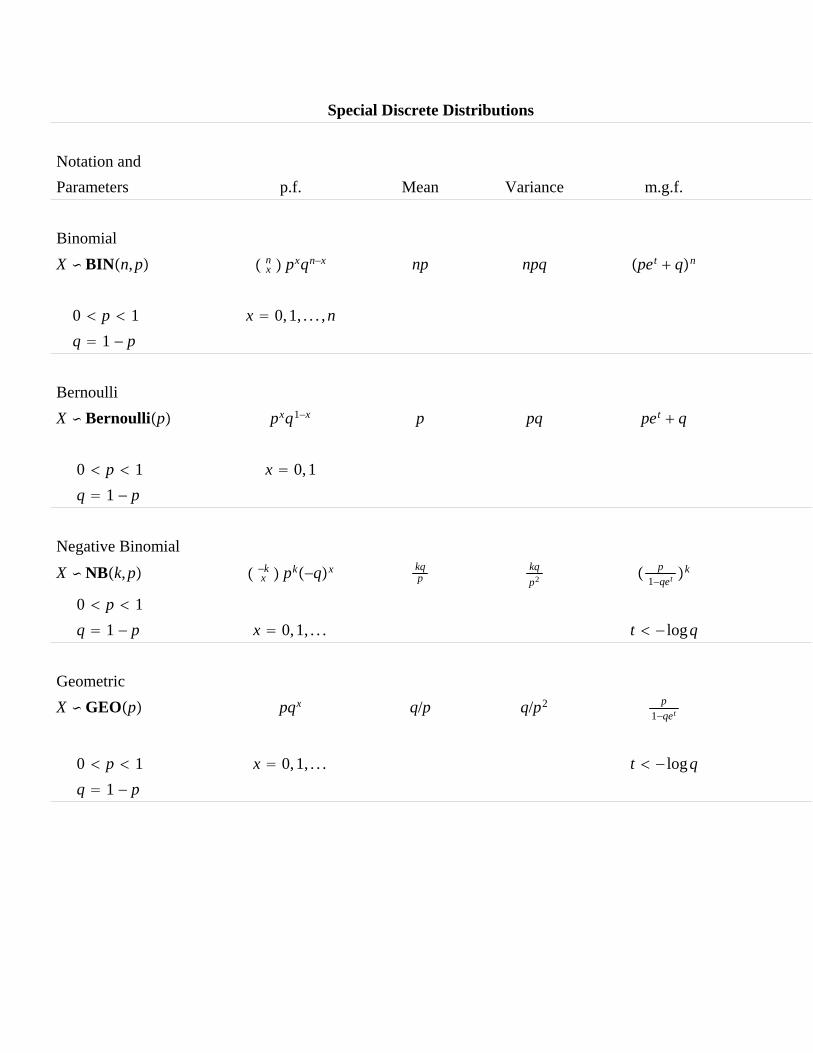
Special Discrete Distributions
Notation andParameters p.f. Mean Variance m.g.f.
BinomialX BINn,p n
x pxqn−x np npq pet qn
0 p 1 x 0,1, . . . ,nq 1 − p
BernoulliX Bernoullip pxq1−x p pq pet q
0 p 1 x 0,1q 1 − p
Negative BinomialX NBk,p −k
x pk−qx kqp
kqp2 p
1−qet k
0 p 1q 1 − p x 0,1, . . . t − logq
GeometricX GEOp pqx q/p q/p2 p
1−qet
0 p 1 x 0,1, . . . t − logqq 1 − p
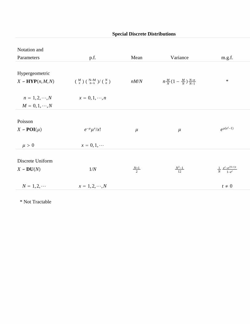
Special Discrete Distributions
Notation andParameters p.f. Mean Variance m.g.f.
HypergeometricX HYPn,M,N M
x N−Mn−x / N
n nM/N n MN 1 −
MN
N−nN−1 *
n 1,2,,N x 0,1,,nM 0,1,,N
PoissonX POI e−x/x! eet−1
0 x 0,1,
Discrete Uniform
X DUN 1/N N12
N2−112
1N
et−eN1t
1−et
N 1,2, x 1,2,,N t ≠ 0
* Not Tractable
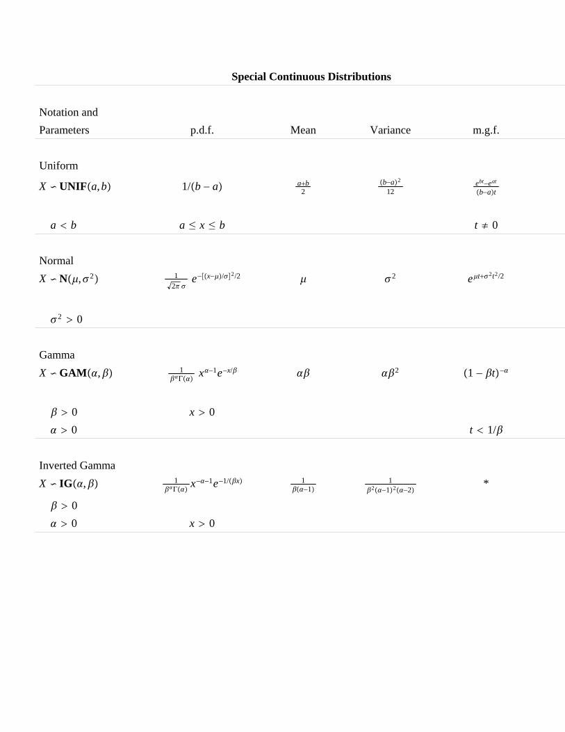
Special Continuous Distributions
Notation andParameters p.d.f. Mean Variance m.g.f.
Uniform
X UNIFa,b 1/b − a ab2
b−a2
12ebt−eat
b−at
a b a ≤ x ≤ b t ≠ 0
NormalX N,2 1
2 e−x−/2/2 2 et2t2/2
2 0
GammaX GAM, 1
Γx−1e−x/ 2 1 − t−
0 x 0 0 t 1/
Inverted GammaX IG, 1
Γx−−1e−1/x 1
−11
2−12−2*
0 0 x 0
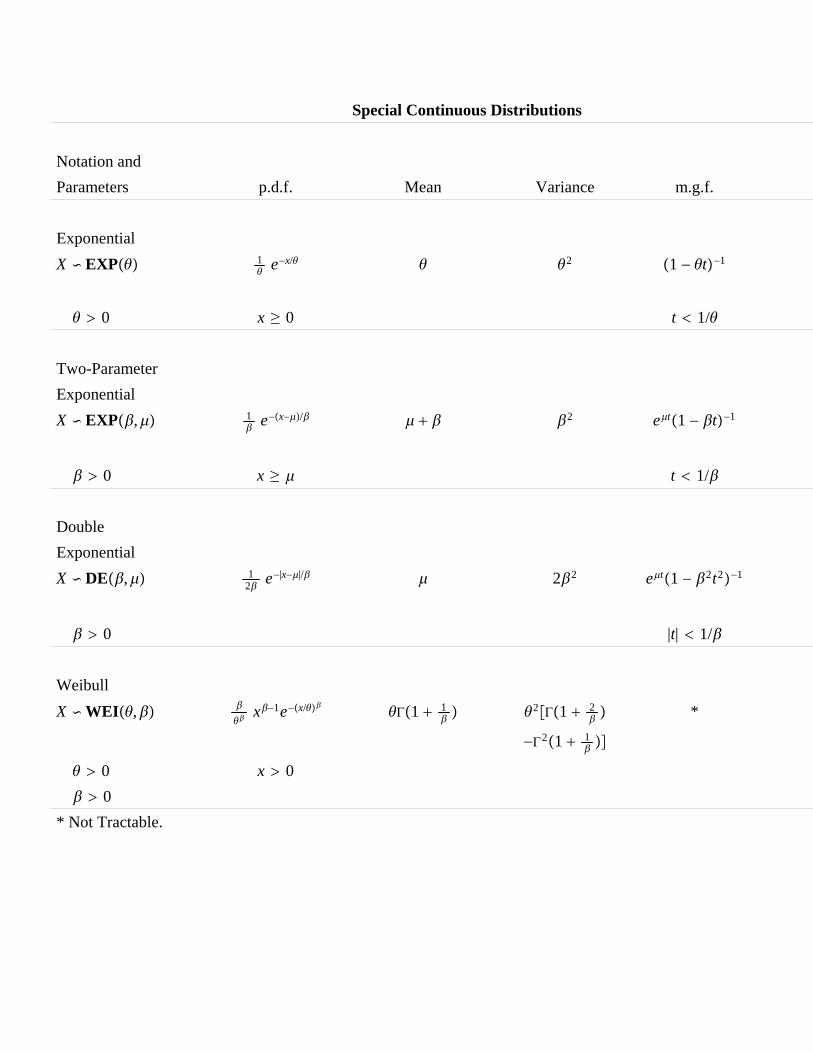
Special Continuous Distributions
Notation andParameters p.d.f. Mean Variance m.g.f.
ExponentialX EXP 1
e−x/ 2 1 − t−1
0 x ≥ 0 t 1/
Two-ParameterExponentialX EXP, 1
e−x−/ 2 et1 − t−1
0 x ≥ t 1/
DoubleExponentialX DE, 1
2 e−|x−|/ 22 et1 − 2t2−1
0 |t| 1/
WeibullX WEI,
x−1e−x/ Γ1 1
2Γ1 2 *
−Γ21 1
0 x 0 0
* Not Tractable.
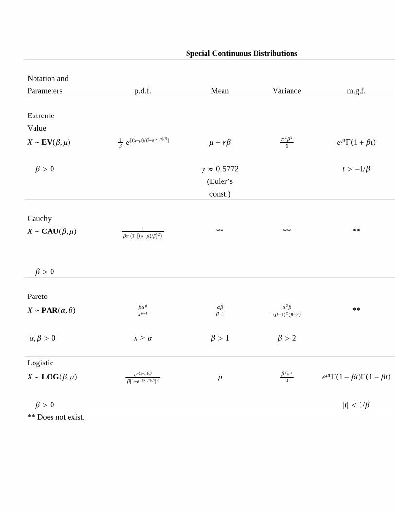
Special Continuous Distributions
Notation andParameters p.d.f. Mean Variance m.g.f.
ExtremeValue
X EV, 1 ex−/−ex−/ − 22
6 etΓ1 t
0 0.5772 t −1/(Euler’sconst.)
CauchyX CAU, 1
1x−/2** ** **
0
Pareto
X PAR,
x1−1
2−12−2
**
, 0 x ≥ 1 2
Logistic
X LOG, e−x−/
1e−x−/2 22
3 etΓ1 − tΓ1 t
0 |t| 1/** Does not exist.
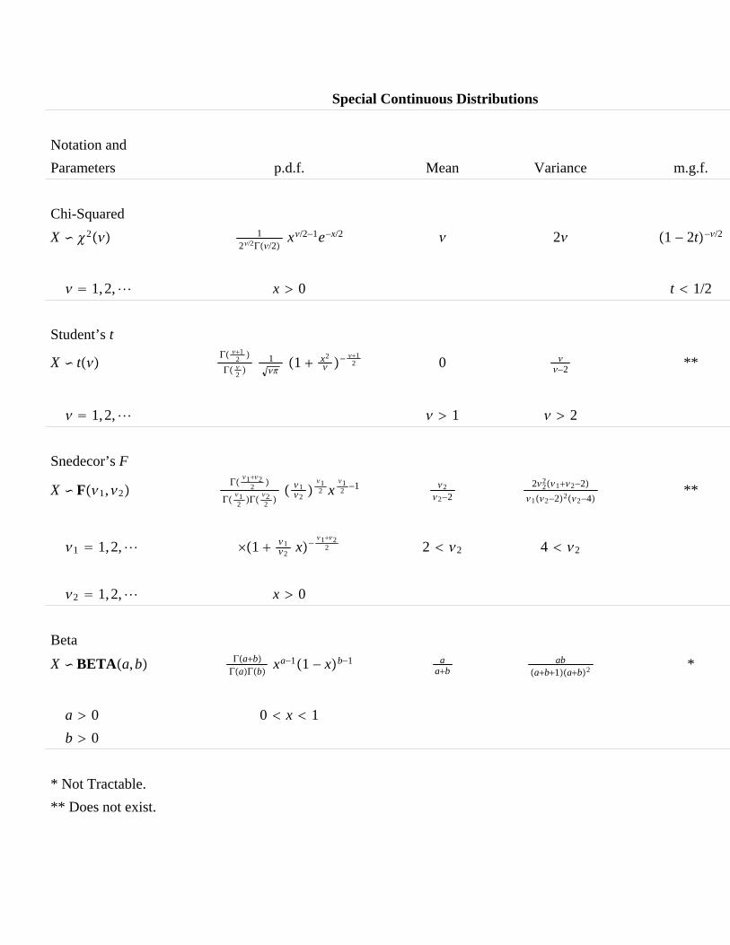
Special Continuous Distributions
Notation andParameters p.d.f. Mean Variance m.g.f.
Chi-SquaredX 2 1
2/2Γ/2x/2−1e−x/2 2 1 − 2t−/2
1,2, x 0 t 1/2
Student’s t
X t Γ 12
Γ 2 1
1 x2 − 1
2 0 −2 **
1,2, 1 2
Snedecor’s F
X F1,2Γ
122
Γ12 Γ
22
12
12 x
12 −1 2
2−222
212−212−222−4
**
1 1,2, 1 12 x−
122 2 2 4 2
2 1,2, x 0
Beta
X BETAa,b ΓabΓaΓb xa−11 − xb−1 a
abab
ab1ab2 *
a 0 0 x 1b 0
* Not Tractable.** Does not exist.
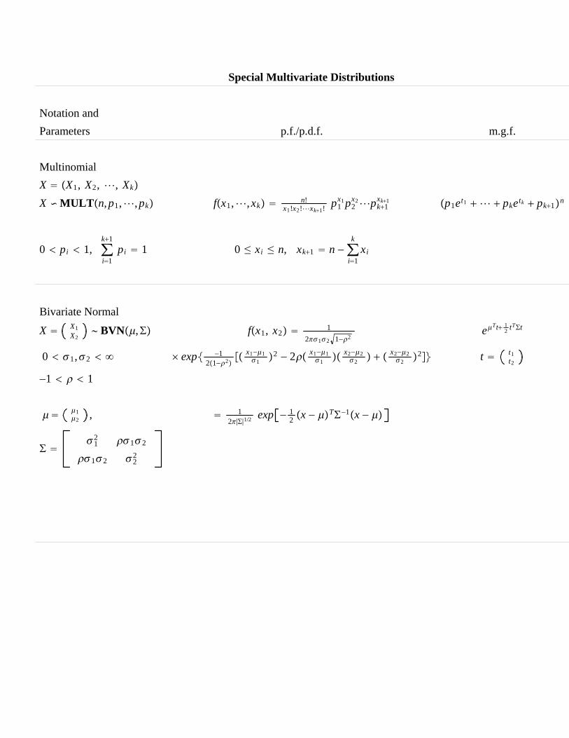
Special Multivariate Distributions
Notation andParameters p.f./p.d.f. m.g.f.
MultinomialX X1, X2, , Xk
X MULTn,p1,,pk fx1,,xk n!x1!x2!xk1! p1
x1p2x2pk1
xk1 p1et1 pketk pk1n
0 pi 1, ∑i1
k1pi 1 0 ≤ xi ≤ n, xk1 n − ∑
i1
kxi
Bivariate Normal
X X1X2
BVN, fx1, x2 1212 1−2
eTt 12 tTt
0 1,2 exp −121−2
x1−11 2 − 2 x1−1
1 x2−22 x2−2
2 2 t t1t2
−1 1
12 , 1
2||1/2 exp − 12 x −
T−1x −
1
2 12
12 22