Embed Size (px)
Citation preview
Statistics 303
Chapter 7Inference for Means
Inference for Means
• To this point, when examining the mean of a population we have always assumed that the population standard deviation () was known.
• In practice this is seldom the case.• We usually must estimate the population standard
deviation with the sample standard deviation s (for a review of s, see pp. 49-50 of the book).
• When we do this, the sampling distribution of the sample mean is no longer normally distributed, because of the adjustment for estimating with s.
• Thus, instead of using the Z, the standard normal distribution, we must use the appropriate t-distribution.
Inference for Means
• The t-distribution– Although there is only one Z-distribution, there
are many, many t-distributions.– In fact, there is a different t-distribution for
each sample size used.– The shape of each t-distribution is very similar
to the Z-distribution, but is slightly flatter.– The larger the sample size, the closer the t-
distribution is to the Z-distribution.
Inference for Means
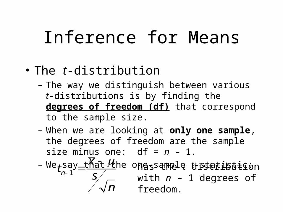
• The t-distribution– The way we distinguish between various t-distributions
is by finding the degrees of freedom (df) that correspond to the sample size.
– When we are looking at only one sample, the degrees of freedom are the sample size minus one: df = n – 1.
– We say that the one-sample t-statistic:
1n
xt
sn
has the t distribution with n – 1
degrees of freedom.
Inference for Means
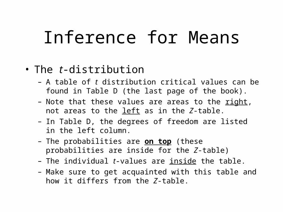
• The t-distribution– A table of t distribution critical values can be found in Table D
(the last page of the book).
– Note that these values are areas to the right, not areas to the left as in the Z-table.
– In Table D, the degrees of freedom are listed in the left column.
– The probabilities are on top (these probabilities are inside for the Z-table)
– The individual t-values are inside the table.
– Make sure to get acquainted with this table and how it differs from the Z-table.
Inference for Means
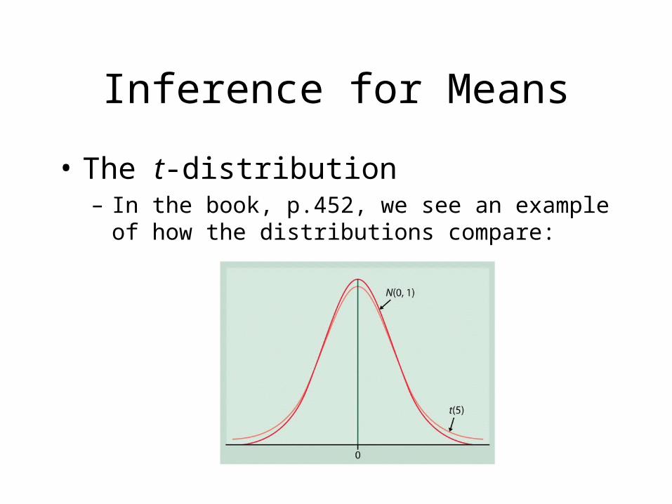
• The t-distribution– In the book, p.452, we see an example of how the
distributions compare:
Inference for Means
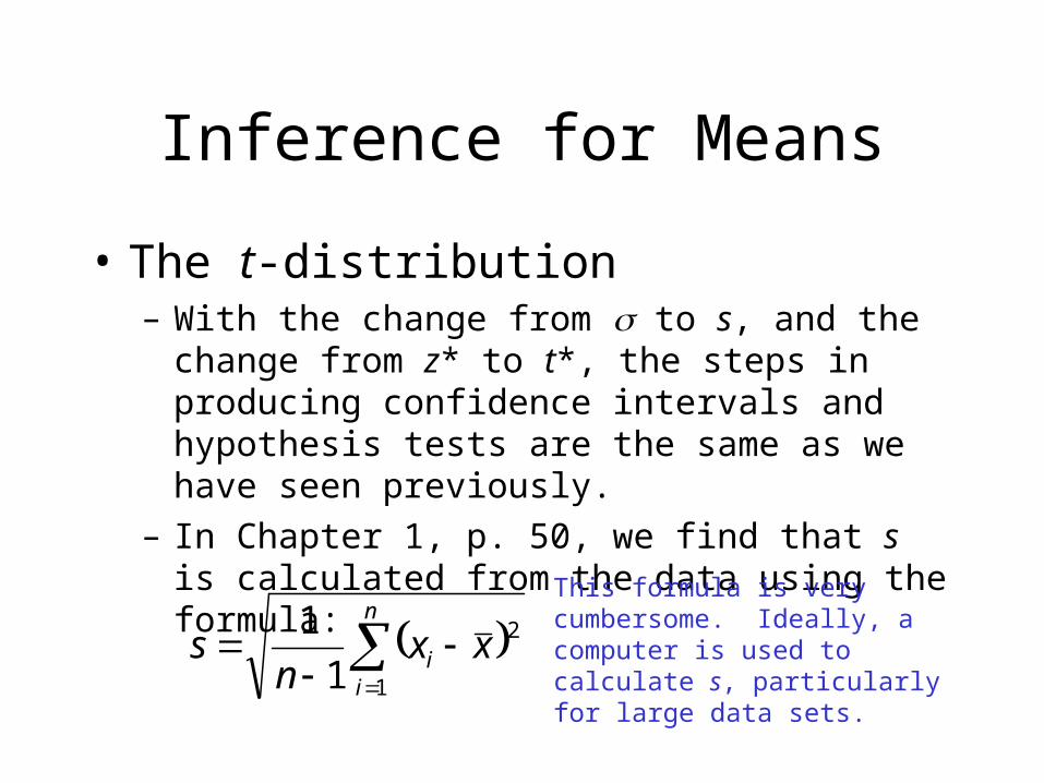
• The t-distribution– With the change from to s, and the change from z* to
t*, the steps in producing confidence intervals and hypothesis tests are the same as we have seen previously.
– In Chapter 1, p. 50, we find that s is calculated from the data using the formula:
n
ii xx
ns
1
2
1
1This formula is very cumbersome. Ideally, a computer is used to calculate s, particularly for large data sets.
Confidence Interval for with Unknown
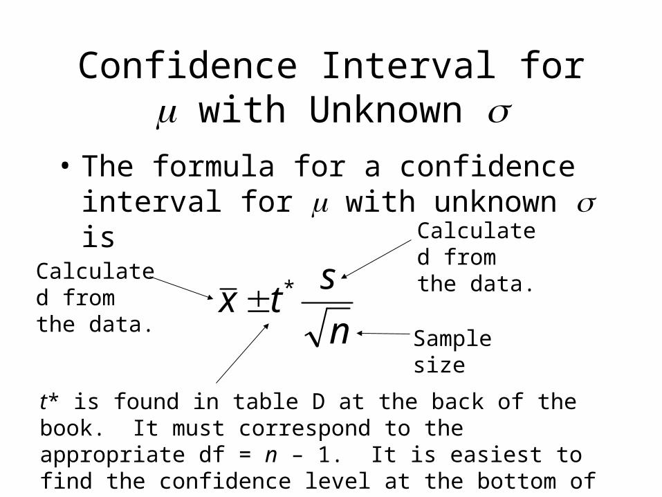
• The formula for a confidence interval for with unknown is
n
stx *
Calculated from the data.
Calculated from the data.
Sample size
t* is found in table D at the back of the book. It must correspond to the appropriate df = n – 1. It is easiest to find the confidence level at the bottom of the table and go up to the correct df.
Confidence Interval for with Unknown
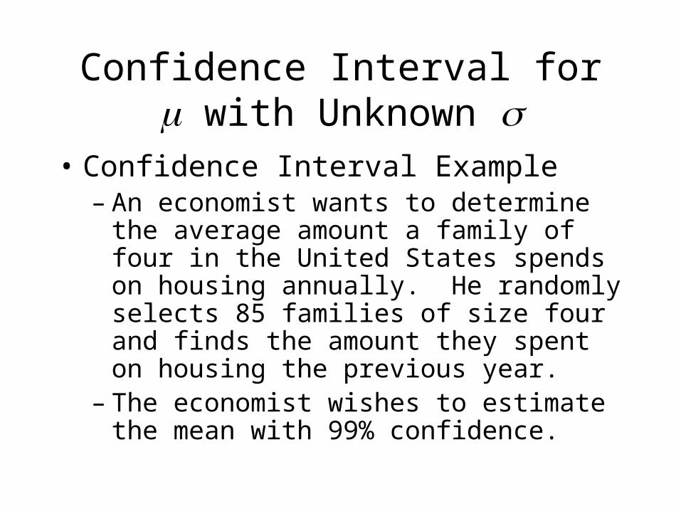
• Confidence Interval Example– An economist wants to determine the average
amount a family of four in the United States spends on housing annually. He randomly selects 85 families of size four and finds the amount they spent on housing the previous year.
– The economist wishes to estimate the mean with 99% confidence.
Confidence Interval for with Unknown
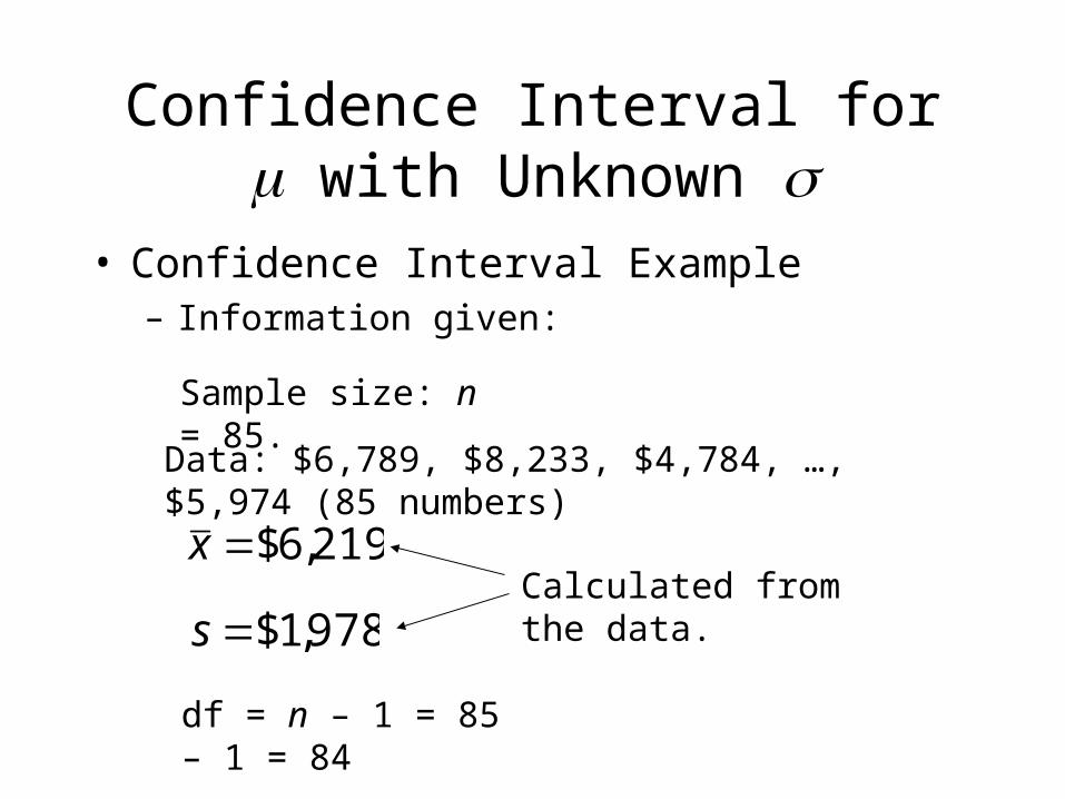
• Confidence Interval Example– Information given:
219,6$x
Sample size: n = 85.
978,1$s
Data: $6,789, $8,233, $4,784, …, $5,974 (85 numbers)
Calculated from the data.
df = n – 1 = 85 – 1 = 84
Confidence Interval for with Unknown
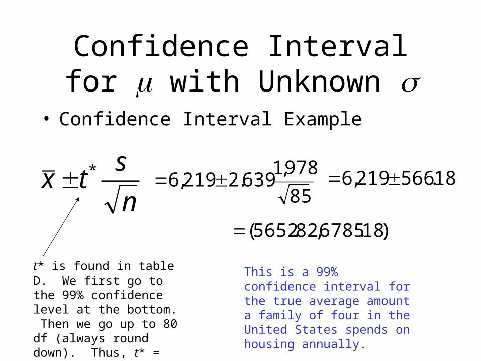
• Confidence Interval Example
n
stx *
t* is found in table D. We first go to the 99% confidence level at the bottom. Then we go up to 80 df (always round down). Thus, t* = 2.639.
85
978,1639.2219,6 18.566219,6
)18.6785,82.5652(
This is a 99% confidence interval for the true average amount a family of four in the United States spends on housing annually.
Hypothesis Test for with Unknown
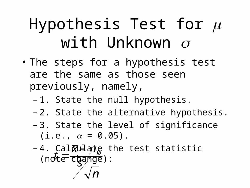
• The steps for a hypothesis test are the same as those seen previously, namely,– 1. State the null hypothesis.– 2. State the alternative hypothesis.– 3. State the level of significance (i.e., = 0.05).– 4. Calculate the test statistic (note change):
ns
xt 0
Hypothesis Test for with Unknown
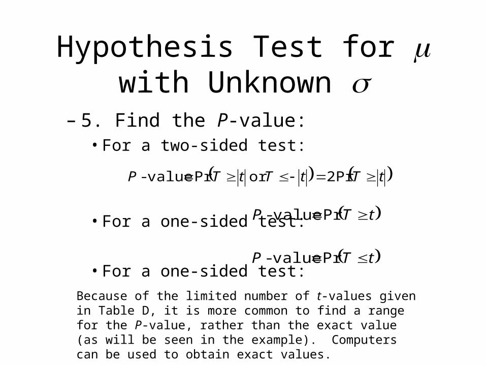
– 5. Find the P-value:• For a two-sided test:
• For a one-sided test:
• For a one-sided test:
tTtTtTP 2Pr or Pr value-
tTP Pr value-
tTP Pr value-
Because of the limited number of t-values given in Table D, it is more common to find a range for the P-value, rather than the exact value (as will be seen in the example). Computers can be used to obtain exact values.
Hypothesis Test for with Unknown
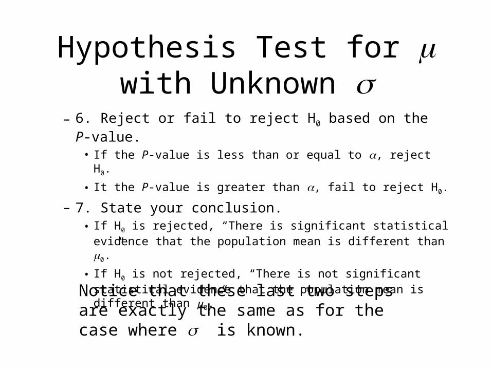
– 6. Reject or fail to reject H0 based on the P-value.
• If the P-value is less than or equal to , reject H0.
• It the P-value is greater than , fail to reject H0.
– 7. State your conclusion.• If H0 is rejected, “There is significant statistical evidence that
the population mean is different than 0.”
• If H0 is not rejected, “There is not significant statistical evidence that the population mean is different than 0.”
Notice that these last two steps are exactly the same as for the case where is known.
Hypothesis Test for with Unknown
• T.V. Example– Suppose that the data collected from our class
survey is a random sample from the entire university (which it obviously is not). We wish to see if there is evidence that the average amount of television watched for students here is more than 7 hours per week.
Hypothesis Test for with Unknown
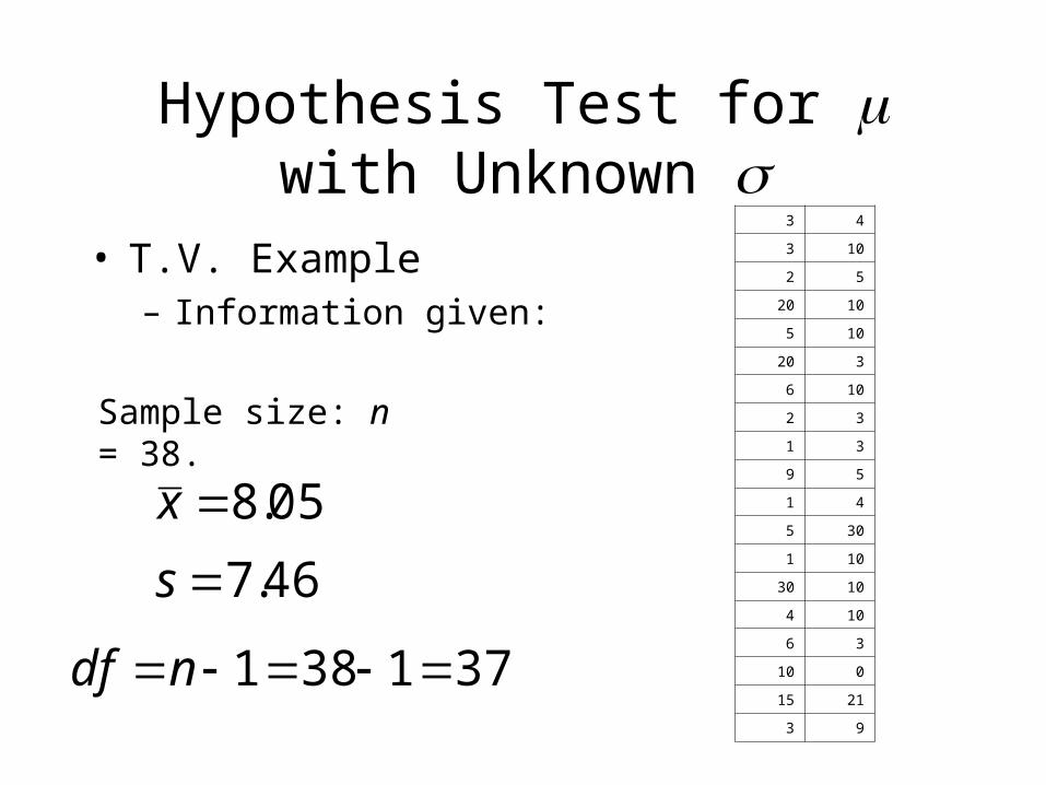
• T.V. Example– Information given:
05.8x
Sample size: n = 38.
3 4
3 10
2 5
20 10
5 10
20 3
6 10
2 3
1 3
9 5
1 4
5 30
1 10
30 10
4 10
6 3
10 0
15 21
3 9
46.7s
371381 ndf
Hypothesis Test for with Unknown
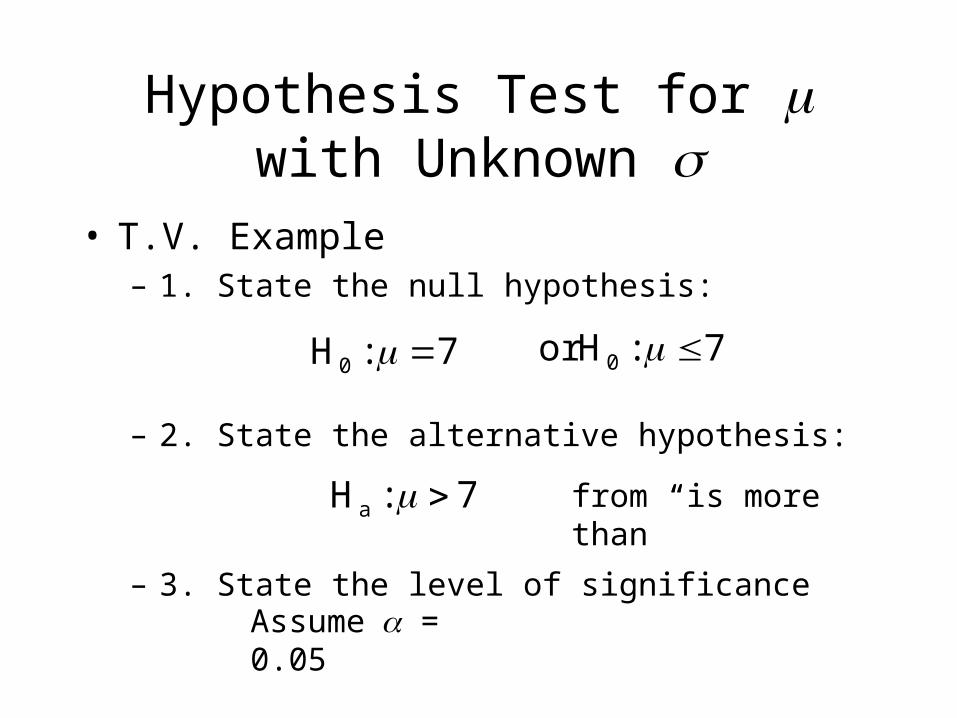
• T.V. Example– 1. State the null hypothesis:
– 2. State the alternative hypothesis:
– 3. State the level of significance
7:H0 7:Hor 0
7:Ha from “is more than”
Assume = 0.05
Hypothesis Test for with Unknown
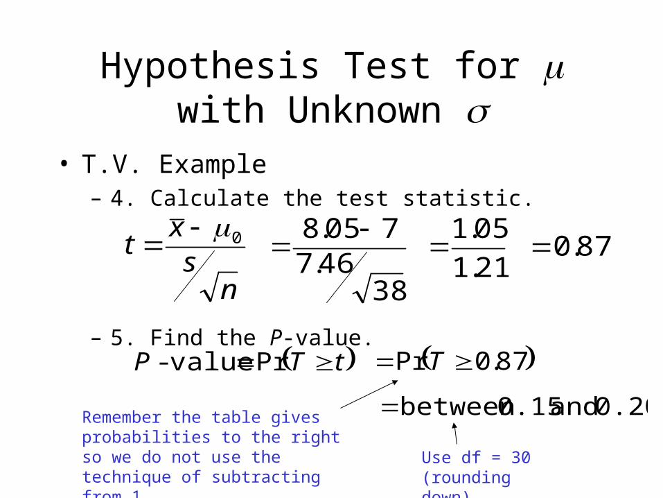
• T.V. Example– 4. Calculate the test statistic.
– 5. Find the P-value.
ns
xt 0
3846.7
705.8
21.1
05.1 87.0
tTP Pr value- 87.0Pr T
0.20 and 0.15between Remember the table gives probabilities to the right so we do not use the technique of subtracting from 1. Use df = 30
(rounding down)
Hypothesis Test for with Unknown
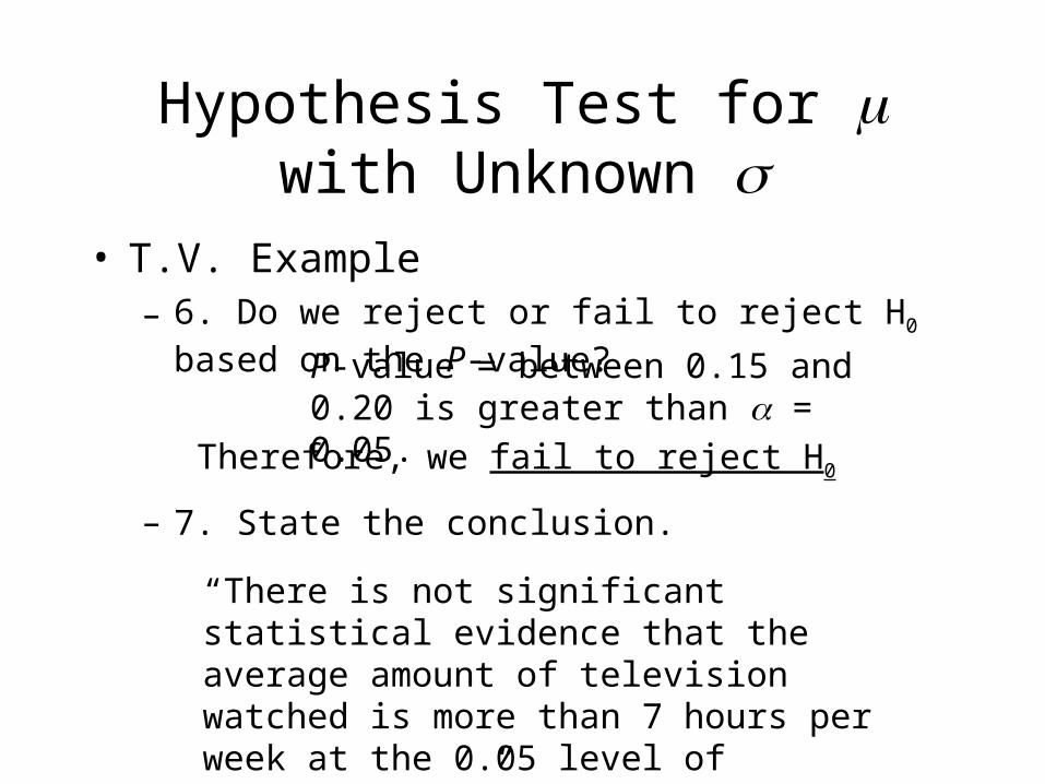
• T.V. Example– 6. Do we reject or fail to reject H0 based on the P-
value?
– 7. State the conclusion.
P-value = between 0.15 and 0.20 is greater than = 0.05.
Therefore, we fail to reject H0
“There is not significant statistical evidence that the average amount of television watched is more than 7 hours per week at the 0.05 level of significance.”
Matched Pairs t-test
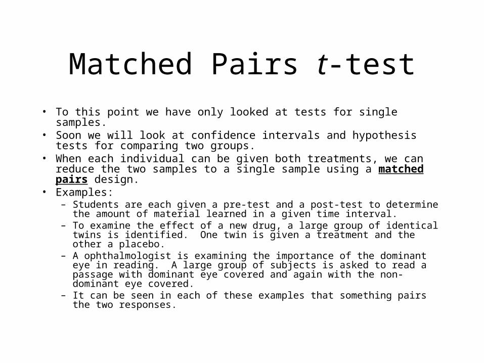
• To this point we have only looked at tests for single samples.• Soon we will look at confidence intervals and hypothesis tests for
comparing two groups.• When each individual can be given both treatments, we can reduce the
two samples to a single sample using a matched pairs design.• Examples:
– Students are each given a pre-test and a post-test to determine the amount of material learned in a given time interval.
– To examine the effect of a new drug, a large group of identical twins is identified. One twin is given a treatment and the other a placebo.
– A ophthalmologist is examining the importance of the dominant eye in reading. A large group of subjects is asked to read a passage with dominant eye covered and again with the non-dominant eye covered.
– It can be seen in each of these examples that something pairs the two responses.
Matched Pairs t-test
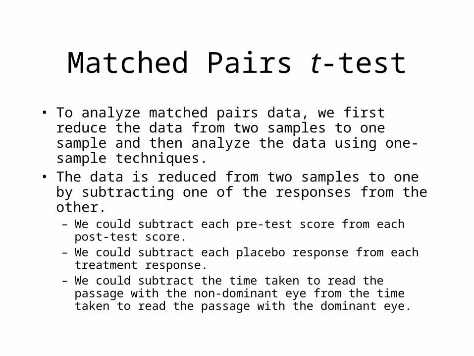
• To analyze matched pairs data, we first reduce the data from two samples to one sample and then analyze the data using one-sample techniques.
• The data is reduced from two samples to one by subtracting one of the responses from the other.– We could subtract each pre-test score from each post-test score.– We could subtract each placebo response from each treatment
response.– We could subtract the time taken to read the passage with the non-
dominant eye from the time taken to read the passage with the dominant eye.
Matched Pairs t-test
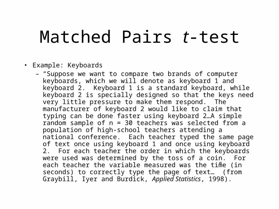
• Example: Keyboards– “Suppose we want to compare two brands of computer keyboards,
which we will denote as keyboard 1 and keyboard 2. Keyboard 1 is a standard keyboard, while keyboard 2 is specially designed so that the keys need very little pressure to make them respond. The manufacturer of keyboard 2 would like to claim that typing can be done faster using keyboard 2…A simple random sample of n = 30 teachers was selected from a population of high-school teachers attending a national conference. Each teacher typed the same page of text once using keyboard 1 and once using keyboard 2. For each teacher the order in which the keyboards were used was determined by the toss of a coin. For each teacher the variable measured was the time (in seconds) to correctly type the page of text…” (from Graybill, Iyer and Burdick, Applied Statistics, 1998).
Matched Pairs t-test
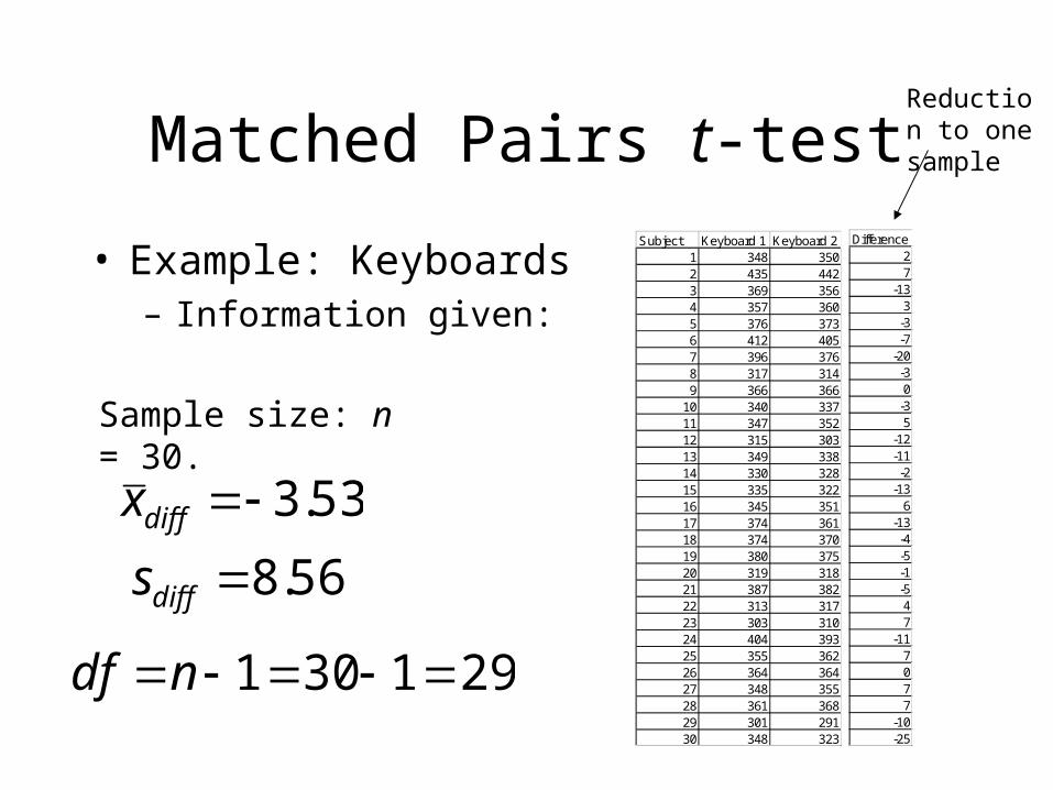
• Example: Keyboards– Information given:
53.3diffx
Sample size: n = 30.
56.8diffs
291301 ndf
Subject Keyboard 1 Keyboard 21 348 3502 435 4423 369 3564 357 3605 376 3736 412 4057 396 3768 317 3149 366 366
10 340 33711 347 35212 315 30313 349 33814 330 32815 335 32216 345 35117 374 36118 374 37019 380 37520 319 31821 387 38222 313 31723 303 31024 404 39325 355 36226 364 36427 348 35528 361 36829 301 29130 348 323
Difference = K2 - K127
-133
-3-7
-20-30
-35
-12-11-2
-136
-13-4-5-1-547
-117077
-10-25
Reduction to one sample
Matched Pairs t-test
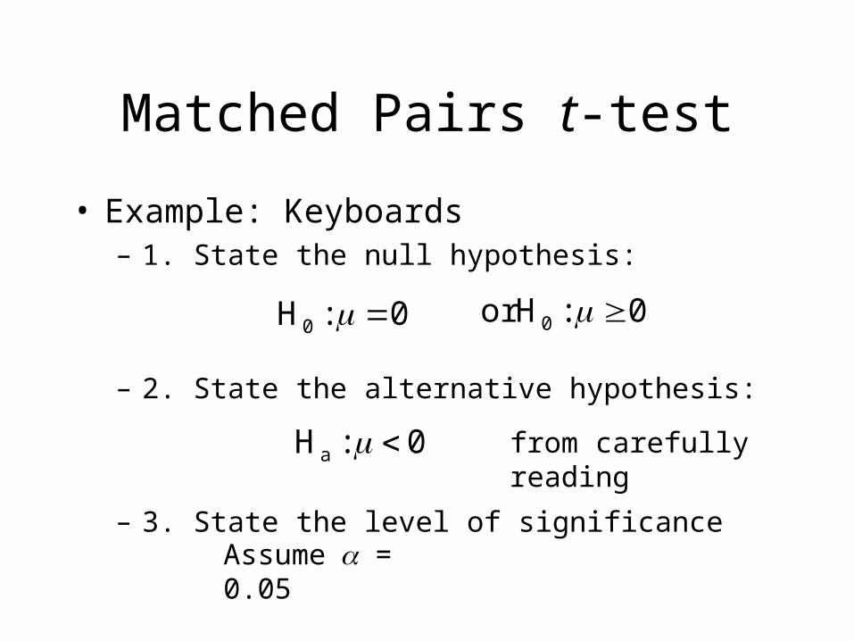
• Example: Keyboards– 1. State the null hypothesis:
– 2. State the alternative hypothesis:
– 3. State the level of significance
0:H0 0:Hor 0
0:Ha from carefully reading
Assume = 0.05
Matched Pairs t-test
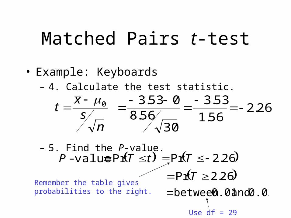
• Example: Keyboards– 4. Calculate the test statistic.
– 5. Find the P-value.
ns
xt 0
3056.8
053.3
56.1
53.3 26.2
tTP Pr value- 26.2Pr T
0.02 and 0.01between Remember the table gives probabilities to the right.
Use df = 29
26.2Pr T
Matched Pairs t-test
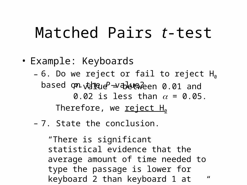
• Example: Keyboards– 6. Do we reject or fail to reject H0 based on the P-
value?
– 7. State the conclusion.
P-value = between 0.01 and 0.02 is less than = 0.05.
Therefore, we reject H0
“There is significant statistical evidence that the average amount of time needed to type the passage is lower for keyboard 2 than keyboard 1 at the 0.05 level of significance.”
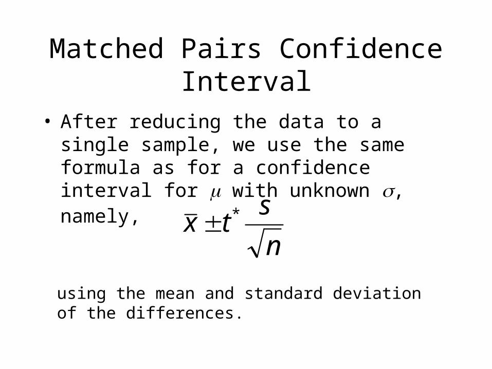
Matched Pairs Confidence Interval
• After reducing the data to a single sample, we use the same formula as for a confidence interval for with unknown , namely,
n
stx *
using the mean and standard deviation of the differences.
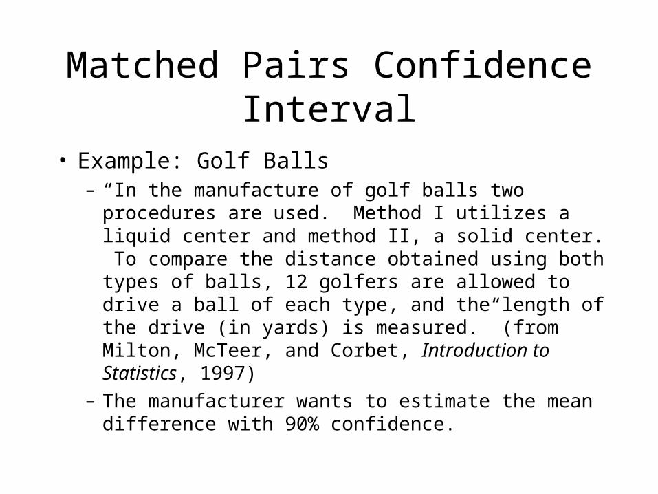
Matched Pairs Confidence Interval
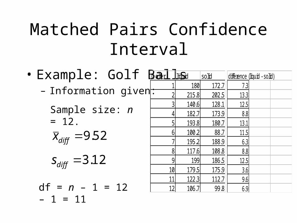
• Example: Golf Balls– “In the manufacture of golf balls two procedures are
used. Method I utilizes a liquid center and method II, a solid center. To compare the distance obtained using both types of balls, 12 golfers are allowed to drive a ball of each type, and the length of the drive (in yards) is measured.” (from Milton, McTeer, and Corbet, Introduction to Statistics, 1997)
– The manufacturer wants to estimate the mean difference with 90% confidence.
Matched Pairs Confidence Interval
• Example: Golf Balls– Information given:
52.9diffx
Sample size: n = 12.
12.3diffs
df = n – 1 = 12 – 1 = 11
Golfer liquid solid1 180 172.72 215.8 202.53 140.6 128.14 182.7 173.95 193.8 180.76 100.2 88.77 195.2 188.98 117.6 108.89 199 186.5
10 179.5 175.911 122.3 112.712 106.7 99.8
difference (liquid - solid)7.3
13.312.58.8
13.111.56.38.8
12.53.69.66.9
Matched Pairs Confidence Interval
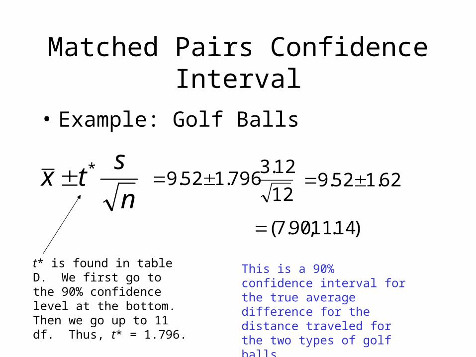
• Example: Golf Balls
n
stx *
t* is found in table D. We first go to the 90% confidence level at the bottom. Then we go up to 11 df. Thus, t* = 1.796.
12
12.3796.152.9 62.152.9
)14.11,90.7(
This is a 90% confidence interval for the true average difference for the distance traveled for the two types of golf balls.
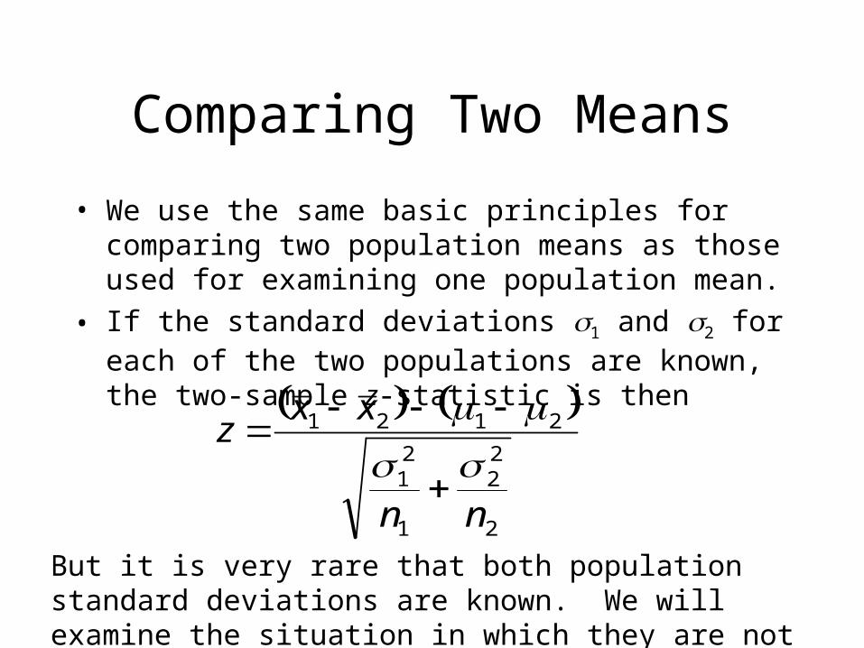
Comparing Two Means
• We use the same basic principles for comparing two population means as those used for examining one population mean.
• If the standard deviations 1 and 2 for each of the two populations are known, the two-sample z-statistic is then
2
22
1
21
2121
nn
xxz
But it is very rare that both population standard deviations are known. We will examine the situation in which they are not known.
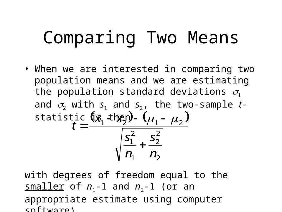
Comparing Two Means
• When we are interested in comparing two population means and we are estimating the population standard deviations 1 and 2 with s1 and s2, the two-sample t-statistic is then
2
22
1
21
2121
ns
ns
xxt
with degrees of freedom equal to the smaller of n1-1 and n2-1 (or an appropriate estimate using computer software).
Comparing Two Means
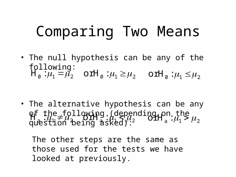
• The null hypothesis can be any of the following:
• The alternative hypothesis can be any of the following (depending on the question being asked):
210 :H 210 :Hor 210 :Hor
21a :H 21a :Hor 21a :Hor
The other steps are the same as those used for the tests we have looked at previously.
Comparing Two Means
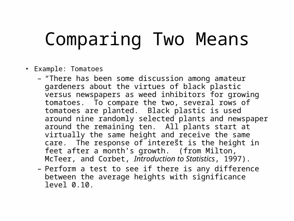
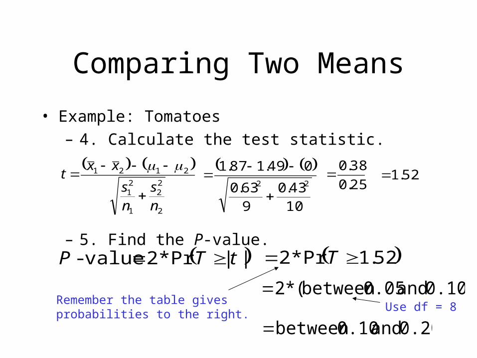
• Example: Tomatoes
– “There has been some discussion among amateur gardeners about the virtues of black plastic versus newspapers as weed inhibitors for growing tomatoes. To compare the two, several rows of tomatoes are planted. Black plastic is used around nine randomly selected plants and newspaper around the remaining ten. All plants start at virtually the same height and receive the same care. The response of interest is the height in feet after a month’s growth.” (from Milton, McTeer, and Corbet, Introduction to Statistics, 1997).
– Perform a test to see if there is any difference between the average heights with significance level 0.10.
Comparing Two Means
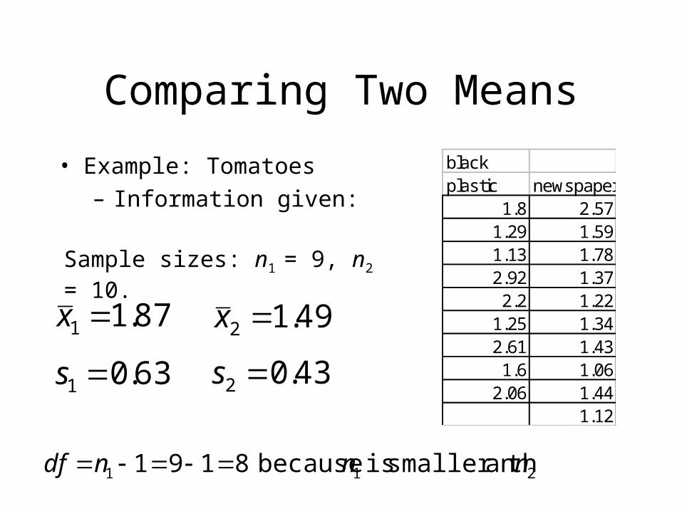
• Example: Tomatoes
– Information given:
87.11 x
Sample sizes: n1 = 9, n2 = 10.
63.01 s
211 an smaller th is because 8191 nnndf
blackplastic newspaper
1.8 2.571.29 1.591.13 1.782.92 1.372.2 1.22
1.25 1.342.61 1.431.6 1.06
2.06 1.441.12
49.12 x
43.02 s
Comparing Two Means
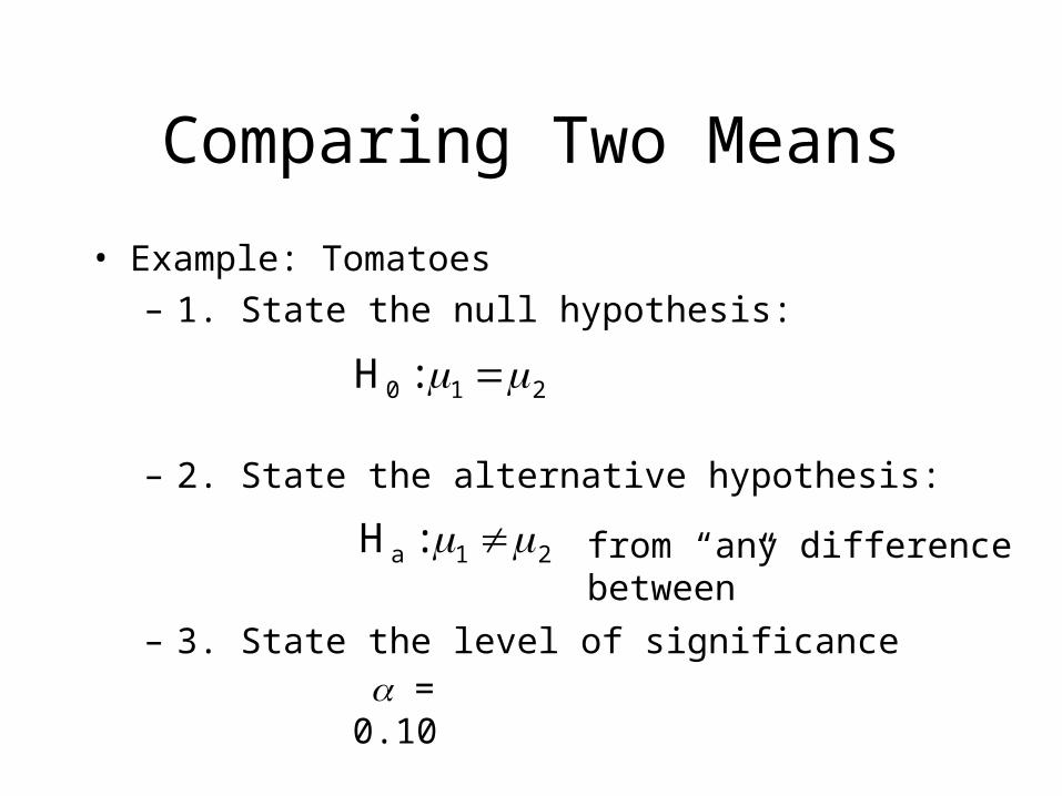
• Example: Tomatoes
– 1. State the null hypothesis:
– 2. State the alternative hypothesis:
– 3. State the level of significance
from “any difference between”
= 0.10
210 :H
21a :H
Comparing Two Means
• Example: Tomatoes
– 4. Calculate the test statistic.
– 5. Find the P-value.
||Pr*2 value- tTP
0.10) and 0.05between (*2Remember the table gives probabilities to the right.
Use df = 8
2
22
1
21
2121
ns
ns
xxt
1043.0
963.0
049.187.122
25.0
38.0 52.1
52.1Pr*2 T
0.20 and 0.10between
Comparing Two Means
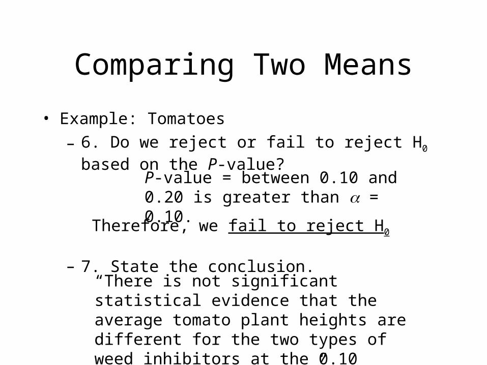
• Example: Tomatoes
– 6. Do we reject or fail to reject H0 based on the P-value?
– 7. State the conclusion.
P-value = between 0.10 and 0.20 is greater than = 0.10.
Therefore, we fail to reject H0
“There is not significant statistical evidence that the average tomato plant heights are different for the two types of weed inhibitors at the 0.10 level of significance.”
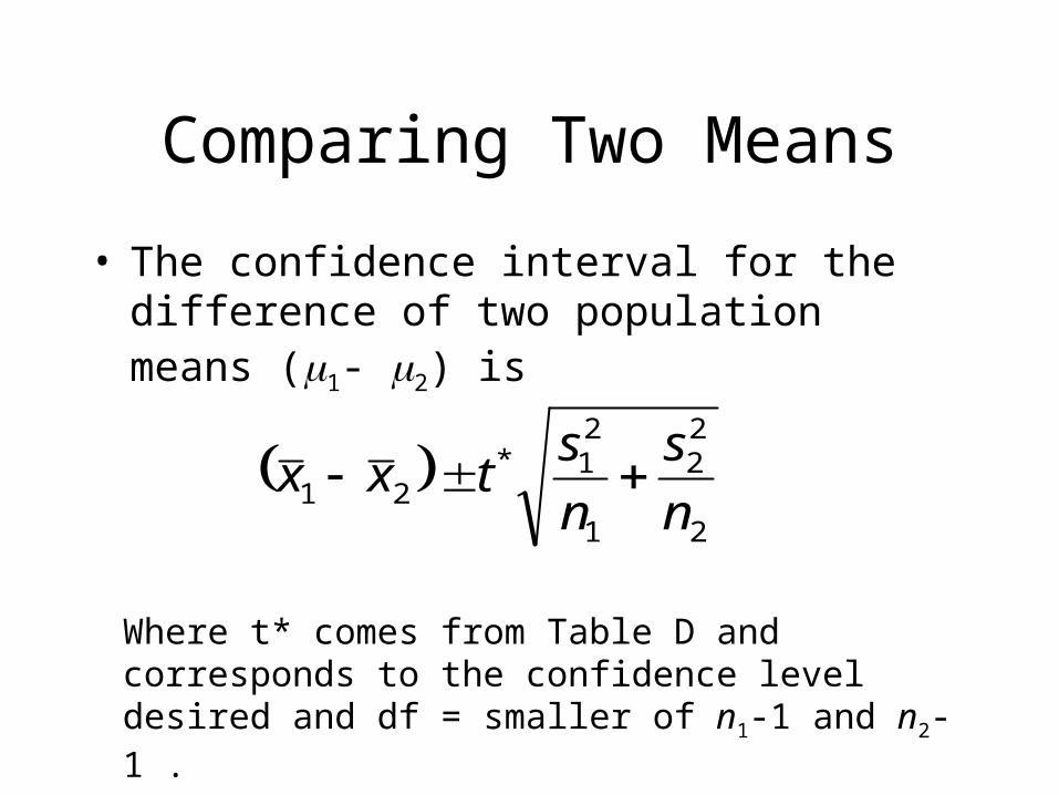
Comparing Two Means
• The confidence interval for the difference of two population means (1- 2) is
Where t* comes from Table D and corresponds to the confidence level desired and df = smaller of n1-1 and n2-1 .
2
22
1
21*
21 n
s
n
stxx
Comparing Two Means
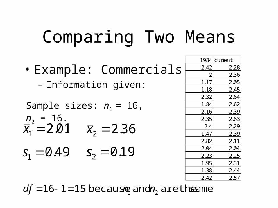
• Example: Commercials– “There is some concern that TV commercial breaks are
becoming longer. The observations on the following slide are obtained on the length in minutes of commercial breaks for the 1984 viewing season and the current season.” (from Milton, McTeer, and Corbet, Introduction to Statistics, 1997)
– Find a 95% confidence interval for the difference between the true averages of the two seasons.
Comparing Two Means
• Example: Commercials– Information given:
1984 current2.42 2.28
2 2.361.17 2.051.18 2.452.32 2.641.84 2.622.16 2.392.35 2.632.4 2.29
1.47 2.392.82 2.112.04 2.042.23 2.251.95 2.311.38 2.442.42 2.57
01.21 x
Sample sizes: n1 = 16, n2 = 16.
49.01 s
same. theare and because 15116 21 nndf
36.22 x
19.02 s
Comparing Two Means
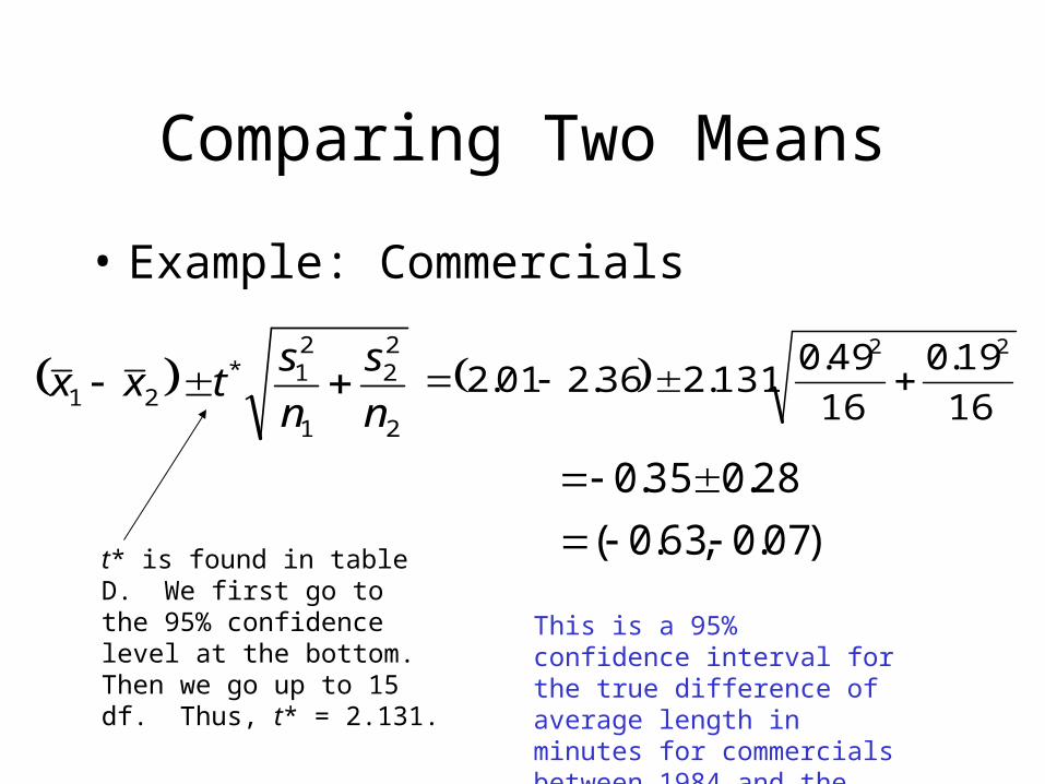
• Example: Commercials
t* is found in table D. We first go to the 95% confidence level at the bottom. Then we go up to 15 df. Thus, t* = 2.131.
28.035.0 )07.0,63.0(
This is a 95% confidence interval for the true difference of average length in minutes for commercials between 1984 and the present.
2
22
1
21*
21 n
s
n
stxx
16
19.0
16
49.0131.236.201.2
22
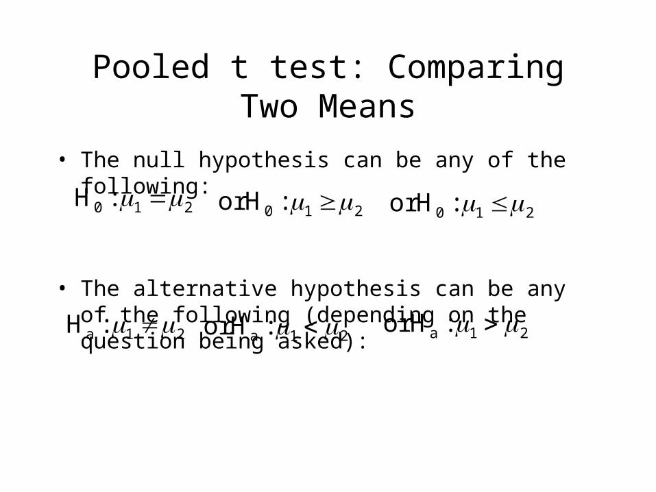
Pooled t test: Comparing Two Means
• The null hypothesis can be any of the following:
• The alternative hypothesis can be any of the following (depending on the question being asked):
210 :H 210 :Hor 210 :Hor
21a :H 21a :Hor 21a :Hor
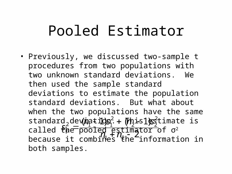
Pooled Estimator
• Previously, we discussed two-sample t procedures from two populations with two unknown standard deviations. We then used the sample standard deviations to estimate the population standard deviations. But what about when the two populations have the same standard deviation. This estimate is called the pooled estimator of σ2 because it combines the information in both samples.
2
)1()1(
21
222
2112
nn
snsns p
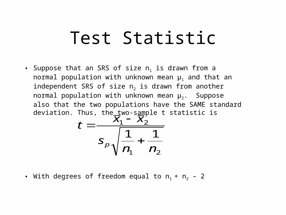
Test Statistic
• Suppose that an SRS of size n1 is drawn from a normal population with unknown mean μ1 and that an independent SRS of size n2 is drawn from another normal population with unknown mean μ2. Suppose also that the two populations have the SAME standard deviation. Thus, the two-sample t statistic is
• With degrees of freedom equal to n1 + n2 – 2
21
21
11nn
s
xxt
p
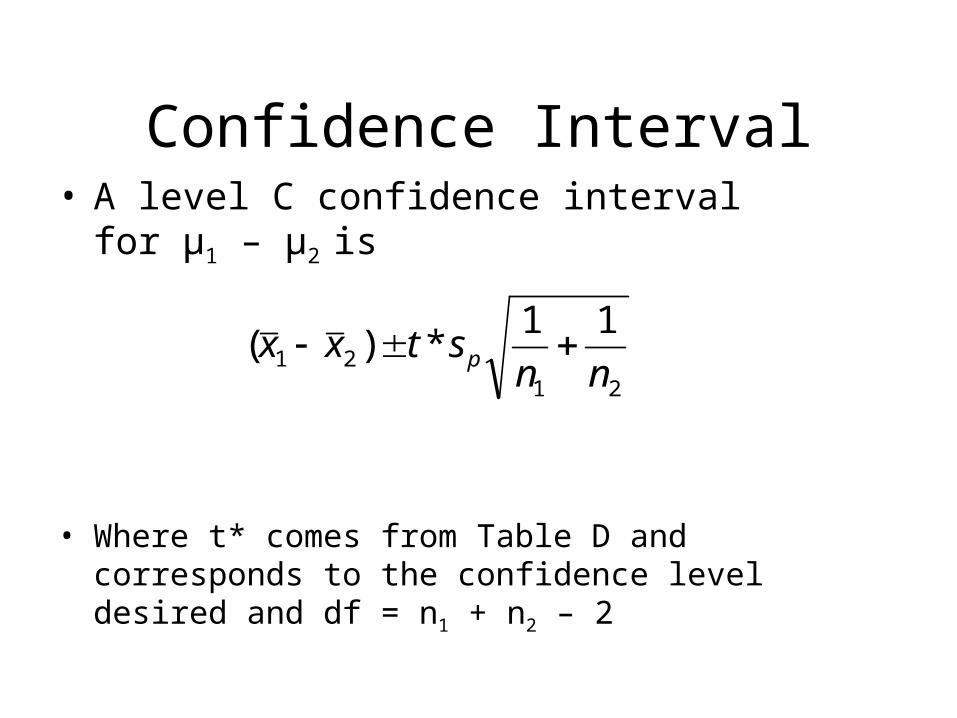
Confidence Interval• A level C confidence interval for μ1 – μ2 is
• Where t* comes from Table D and corresponds to the confidence level desired and df = n1 + n2 – 2
2121
11*)(
nnstxx p