Embed Size (px)
Citation preview
ALAGAPPA UNIVERSITY
[Accredited with ‘A+’ Grade by NAAC (CGPA:3.64) in the Third Cycle and Graded as Category–I University by MHRD-UGC]
(A State University Established by the Government of Tamil Nadu)
KARAIKUDI – 630 003
DIRECTORATE OF DISTANCE EDUCATION
B.Sc. (Mathematics)
IV - Semester
113 44
STATISTICS
Copy rights reserved For private use only
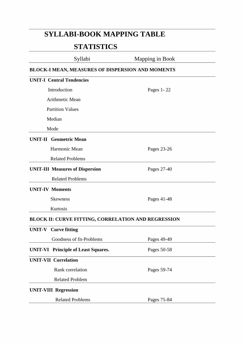
SYLLABI-BOOK MAPPING TABLE
STATISTICS
Syllabi Mapping in Book
BLOCK-I MEAN, MEASURES OF DISPERSION AND MOMENTS
UNIT-I Central Tendencies
Introduction Pages 1- 22
Arithmetic Mean
Partition Values
Median
Mode
UNIT-II Geometric Mean
Harmonic Mean Pages 23-26
Related Problems
UNIT-III Measures of Dispersion Pages 27-40
Related Problems
UNIT-IV Moments
Skewness Pages 41-48
Kurtosis
BLOCK II: CURVE FITTING, CORRELATION AND REGRESSION
UNIT-V Curve fitting
Goodness of fit-Problems Pages 49-49
UNIT-VI Principle of Least Squares. Pages 50-58
UNIT-VII Correlation
Rank correlation Pages 59-74
Related Problem
UNIT-VIII Regression
Related Problems Pages 75-84
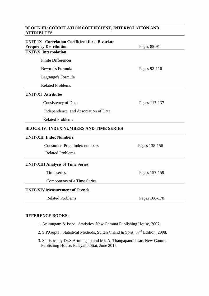
BLOCK III: CORRELATION COEFFICIENT, INTERPOLATION AND
ATTRIBUTES
UNIT-IX Correlation Coefficient for a Bivariate
Frequency Distribution Pages 85-91
UNIT-X Interpolation
Finite Differences
Newton's Formula Pages 92-116
Lagrange's Formula
Related Problems
UNIT-XI Attributes
Consistency of Data Pages 117-137
Independence and Association of Data
Related Problems
BLOCK IV: INDEX NUMBERS AND TIME SERIES
UNIT-XII Index Numbers
Consumer Price Index numbers Pages 138-156
Related Problems
UNIT-XIII Analysis of Time Series
Time series Pages 157-159
Components of a Time Series
UNIT-XIV Measurement of Trends
Related Problems Pages 160-170
REFERENCE BOOKS:
1. Arumugam & Issac , Statistics, New Gamma Publishing House, 2007.
2. S.P.Gupta , Statistical Methods, Sultan Chand & Sons, 37th
Edition, 2008.
3. Statistics by Dr.S.Arumugam and Mr. A. ThangapandiIssac, New Gamma
Publishing House, Palayamkottai, June 2015.
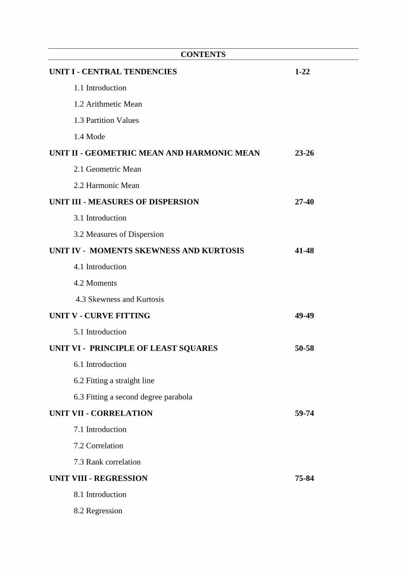
CONTENTS
UNIT I - CENTRAL TENDENCIES 1-22
1.1 Introduction
1.2 Arithmetic Mean
1.3 Partition Values
1.4 Mode
UNIT II - GEOMETRIC MEAN AND HARMONIC MEAN 23-26
2.1 Geometric Mean
2.2 Harmonic Mean
UNIT III - MEASURES OF DISPERSION 27-40
3.1 Introduction
3.2 Measures of Dispersion
UNIT IV - MOMENTS SKEWNESS AND KURTOSIS 41-48
4.1 Introduction
4.2 Moments
4.3 Skewness and Kurtosis
UNIT V - CURVE FITTING 49-49
5.1 Introduction
UNIT VI - PRINCIPLE OF LEAST SQUARES 50-58
6.1 Introduction
6.2 Fitting a straight line
6.3 Fitting a second degree parabola
UNIT VII - CORRELATION 59-74
7.1 Introduction
7.2 Correlation
7.3 Rank correlation
UNIT VIII - REGRESSION 75-84
8.1 Introduction
8.2 Regression
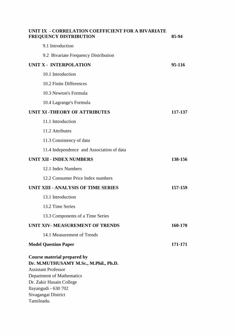
UNIT IX - CORRELATION COEFFICIENT FOR A BIVARIATE
FREQUENCY DISTRIBUTION 85-94
9.1 Introduction
9.2 Bivariate Frequency Distribution
UNIT X - INTERPOLATION 95-116
10.1 Introduction
10.2 Finite Differences
10.3 Newton's Formula
10.4 Lagrange's Formula
UNIT XI -THEORY OF ATTRIBUTES 117-137
11.1 Introduction
11.2 Attributes
11.3 Consistency of data
11.4 Independence and Association of data
UNIT XII - INDEX NUMBERS 138-156
12.1 Index Numbers
12.2 Consumer Price Index numbers
UNIT XIII - ANALYSIS OF TIME SERIES 157-159
13.1 Introduction
13.2 Time Series
13.3 Components of a Time Series
UNIT XIV- MEASUREMENT OF TRENDS 160-170
14.1 Measurement of Trends
Model Question Paper 171-171
Course material prepared by
Dr. M.MUTHUSAMY M.Sc., M.Phil., Ph.D.
Assistant Professor
Department of Mathematics
Dr. Zakir Husain College
Ilayangudi - 630 702
Sivagangai District
Tamilnadu.
1 self - Instructional Material
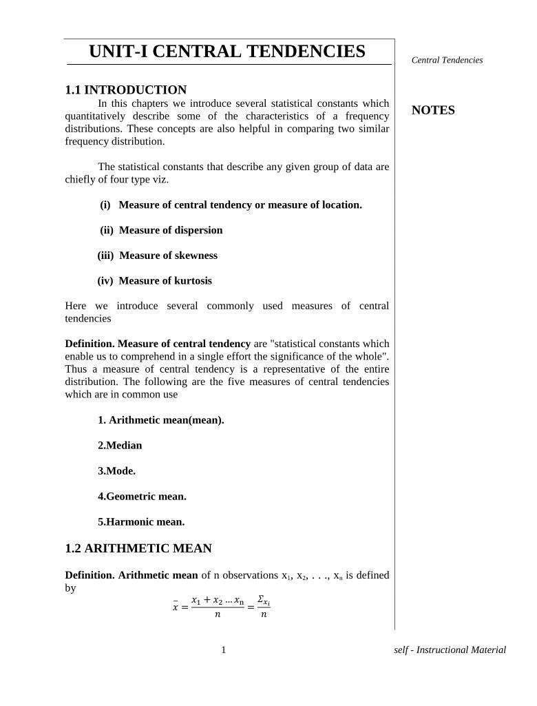
UNIT-I CENTRAL TENDENCIES
1.1 INTRODUCTION In this chapters we introduce several statistical constants which
quantitatively describe some of the characteristics of a frequency
distributions. These concepts are also helpful in comparing two similar
frequency distribution.
The statistical constants that describe any given group of data are
chiefly of four type viz.
(i) Measure of central tendency or measure of location.
(ii) Measure of dispersion
(iii) Measure of skewness
(iv) Measure of kurtosis
Here we introduce several commonly used measures of central
tendencies
Definition. Measure of central tendency are "statistical constants which
enable us to comprehend in a single effort the significance of the whole".
Thus a measure of central tendency is a representative of the entire
distribution. The following are the five measures of central tendencies
which are in common use
1. Arithmetic mean(mean).
2.Median
3.Mode.
4.Geometric mean.
5.Harmonic mean.
1.2 ARITHMETIC MEAN
Definition. Arithmetic mean of n observations x1, x2, . . ., xn is defined
by
Central Tendencies
NOTES
2 self - Instructional Material
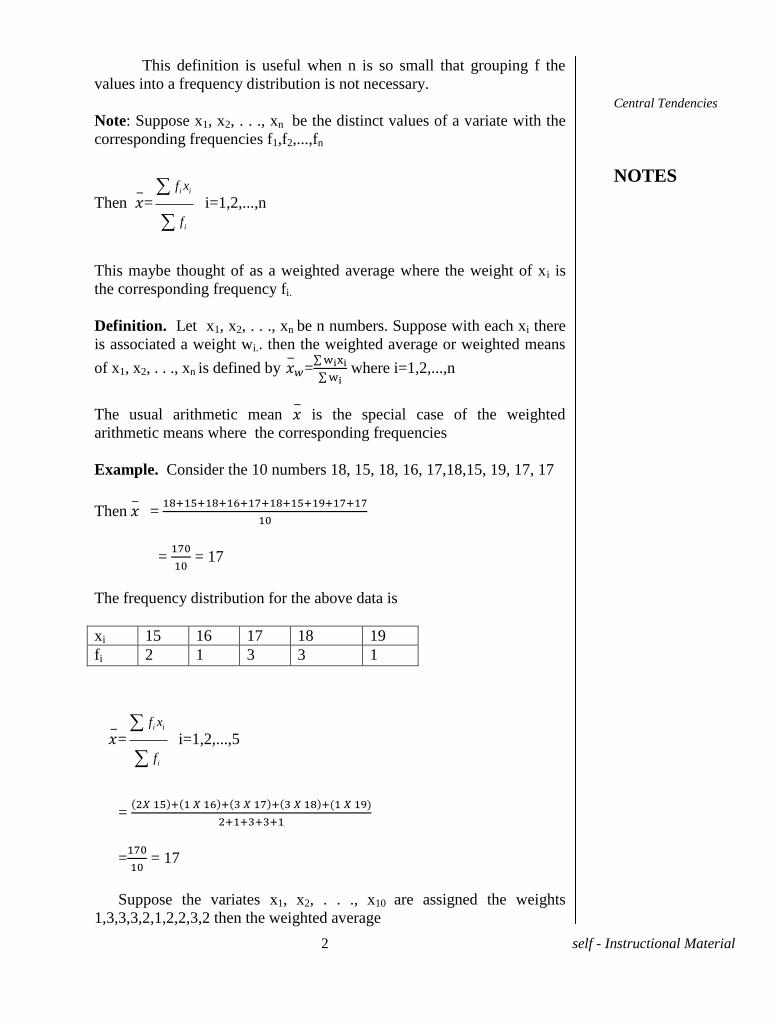
This definition is useful when n is so small that grouping f the
values into a frequency distribution is not necessary.
Note: Suppose x1, x2, . . ., xn be the distinct values of a variate with the
corresponding frequencies f1,f2,...,fn
Then
=i i
i
f x
f
i=1,2,...,n
This maybe thought of as a weighted average where the weight of xi is
the corresponding frequency fi.
Definition. Let x1, x2, . . ., xn be n numbers. Suppose with each xi there
is associated a weight wi.. then the weighted average or weighted means
of x1, x2, . . ., xn is defined by
=
where i=1,2,...,n
The usual arithmetic mean
is the special case of the weighted
arithmetic means where the corresponding frequencies
Example. Consider the 10 numbers 18, 15, 18, 16, 17,18,15, 19, 17, 17
Then =
=
= 17
The frequency distribution for the above data is
xi 15 16 17 18 19
fi 2 1 3 3 1
=i i
i
f x
f
i=1,2,...,5
=
=
= 17
Suppose the variates x1, x2, . . ., x10 are assigned the weights
1,3,3,3,2,1,2,2,3,2 then the weighted average
Central Tendencies
NOTES
3 self - Instructional Material
=
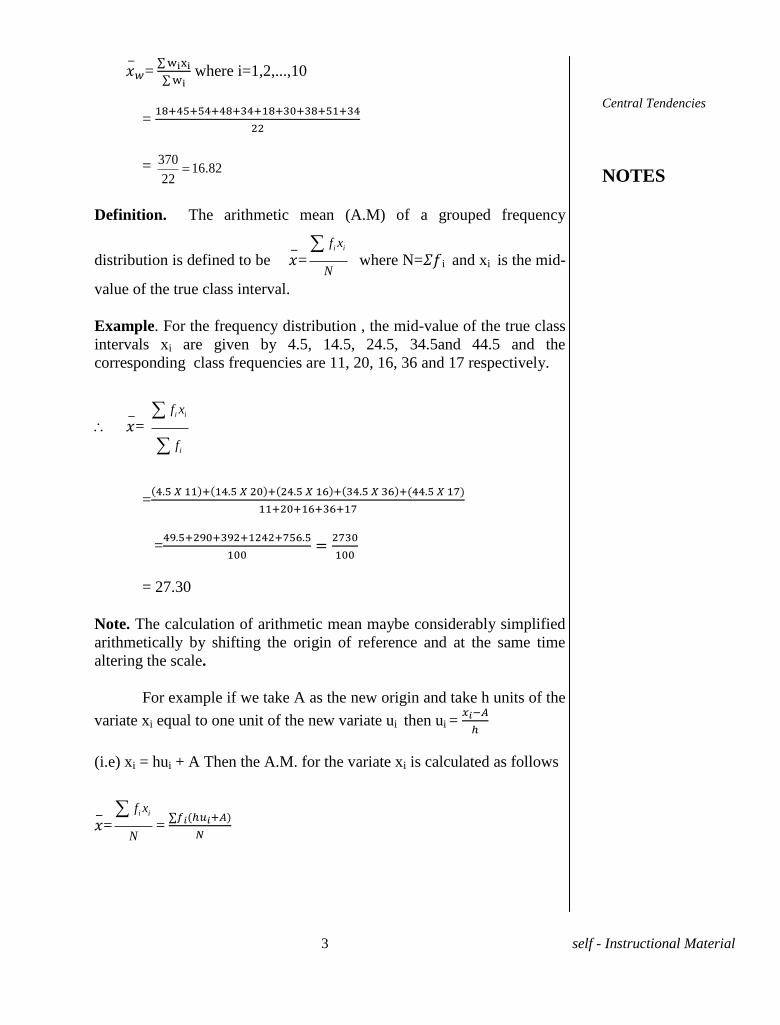
where i=1,2,...,10
=
= 37016.82
22
Definition. The arithmetic mean (A.M) of a grouped frequency
distribution is defined to be
=i if x
N
where N= i and xi is the mid-
value of the true class interval.
Example. For the frequency distribution , the mid-value of the true class
intervals xi are given by 4.5, 14.5, 24.5, 34.5and 44.5 and the
corresponding class frequencies are 11, 20, 16, 36 and 17 respectively.
= i i
i
f x
f
=
=
= 27.30
Note. The calculation of arithmetic mean maybe considerably simplified
arithmetically by shifting the origin of reference and at the same time
altering the scale.
For example if we take A as the new origin and take h units of the
variate xi equal to one unit of the new variate ui then ui =
(i.e) xi = hui + A Then the A.M. for the variate xi is calculated as follows
=i if x
N
=
Central Tendencies
NOTES
4 self - Instructional Material
=h i if u
N
+
if
N
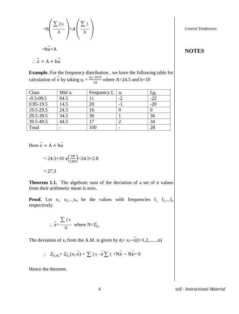
=h
+A
Example. For the frequency distribution , we have the following table for
calculation of
by taking ui =
where A=24.5 and h=10
Class Mid xi Frequency fi ui fiui
-0.5-09.5 04.5 11 -2 -22
0.95-19.5 14.5 20 -1 -20
19.5-29.5 24.5 16 0 0
29.5-39.5 34.5 36 1 36
39.5-49.5 44.5 17 2 34
Total - 100 - 28
Here
= 24.5+10 x
=24.5+2.8
= 27.3
Theorem 1.1. The algebraic sum of the deviation of a set of n values
from their arithmetic mean is zero.
Proof. Let x1, x2,...,xn be the values with frequencies f1, f2,...,fn
respectively.
=i if x
N
where N=
The deviation of xi from the A.M. is given by di= xi
(i=1,2,......,n)
= xi-
) = i if x -
if =N
= 0
Hence the theorem.
Central Tendencies
NOTES
5 self - Instructional Material
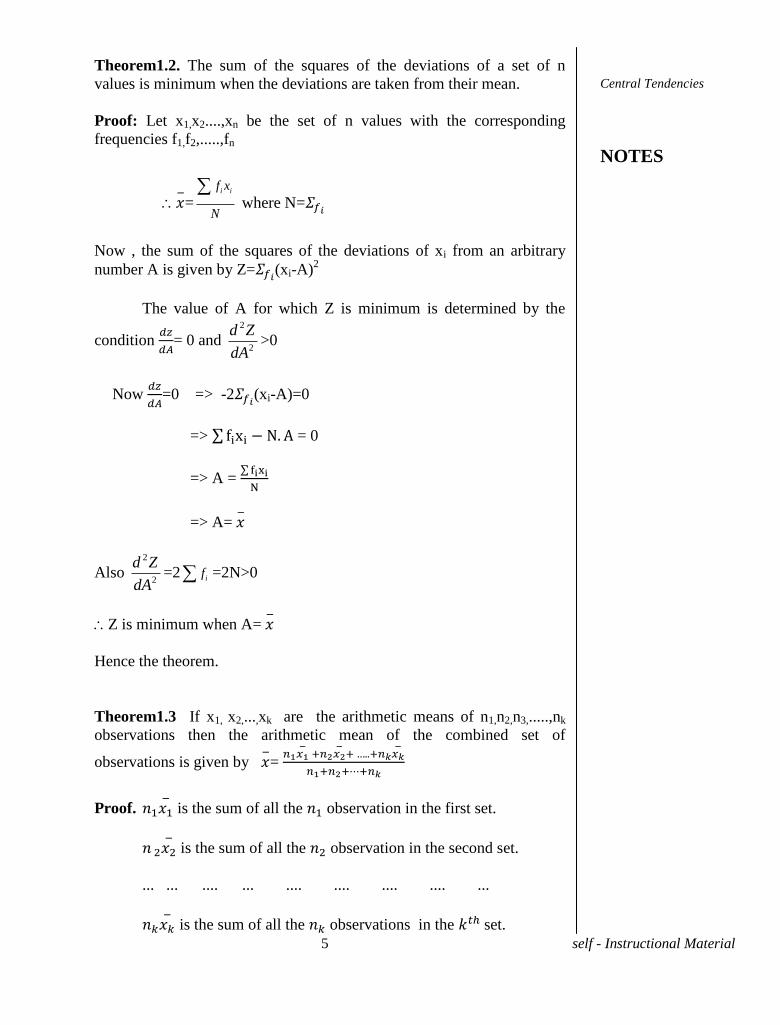
Theorem1.2. The sum of the squares of the deviations of a set of n
values is minimum when the deviations are taken from their mean.
Proof: Let x1,x2....,xn be the set of n values with the corresponding
frequencies f1,f2,.....,fn
=i if x
N
where N=
Now , the sum of the squares of the deviations of xi from an arbitrary
number A is given by Z= (xi-A)2
The value of A for which Z is minimum is determined by the
condition
= 0 and
2
2
d Z
dA>0
Now
=0 => -2 (xi-A)=0
=> = 0
=> A =
=> A=
Also 2
2
d Z
dA=2 if =2N>0
Z is minimum when A=
Hence the theorem.
Theorem1.3 If x1, x2,...,xk are the arithmetic means of n1,n2,n3,.....,nk
observations then the arithmetic mean of the combined set of
observations is given by
=
Proof.
is the sum of all the observation in the first set.
is the sum of all the observation in the second set.
... ... .... ... .... .... .... .... ...
is the sum of all the observations in the set.
Central Tendencies
NOTES
6 self - Instructional Material
1
k
i
is the sum of all the (n1+n2+.....+nk) observations in the
combined set.
=
1
k
i
where N=
1
k
i
. Hence the theorem.
Solved Problems.
Problem 1. The heights of 10 students in c.m's chosen at random are
given by 164, 159, 162, 168, 165, 170, 168, 171, 154, 169 Calculate
A.M.
Solution. Here n=10
=
iX =
(1690) = 169 c.m.
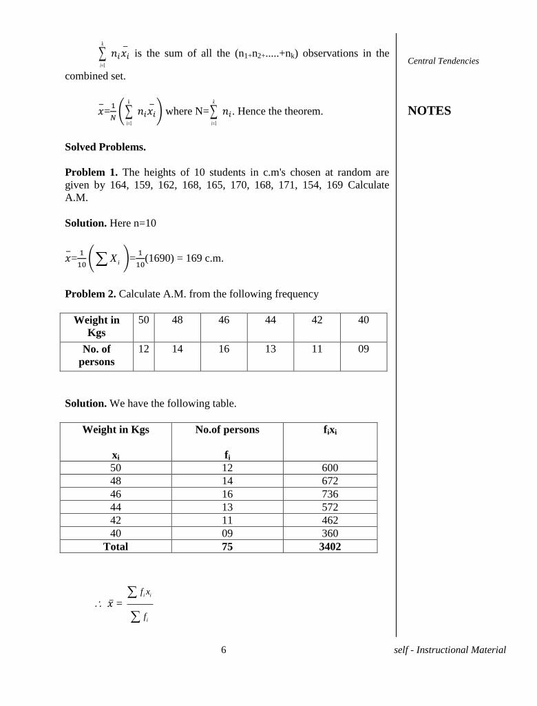
Problem 2. Calculate A.M. from the following frequency
Weight in
Kgs
50 48 46 44 42 40
No. of
persons
12 14 16 13 11 09
Solution. We have the following table.
Weight in Kgs
xi
No.of persons
fi
fixi
50 12 600
48 14 672
46 16 736
44 13 572
42 11 462
40 09 360
Total 75 3402
= i i
i
f x
f
Central Tendencies
NOTES
7 self - Instructional Material
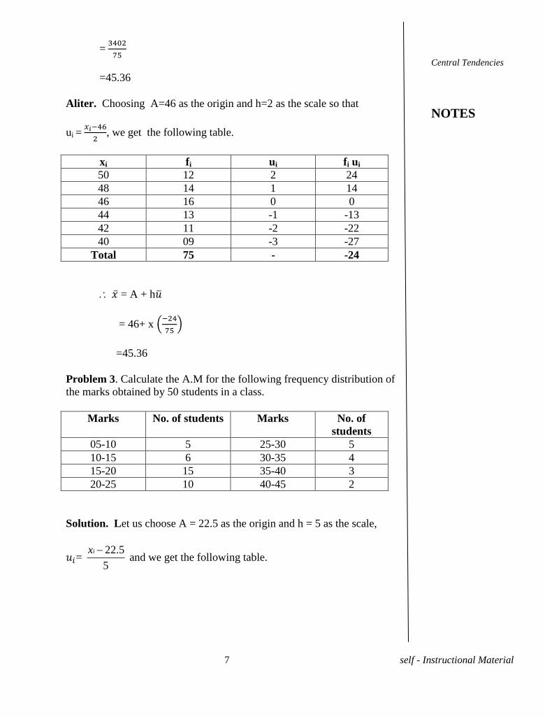
=
=45.36
Aliter. Choosing A=46 as the origin and h=2 as the scale so that
ui =
, we get the following table.
xi fi ui fi ui
50 12 2 24
48 14 1 14
46 16 0 0
44 13 -1 -13
42 11 -2 -22
40 09 -3 -27
Total 75 - -24
= A + h
= 46+ x
=45.36
Problem 3. Calculate the A.M for the following frequency distribution of
the marks obtained by 50 students in a class.
Marks No. of students Marks No. of
students
05-10 5 25-30 5
10-15 6 30-35 4
15-20 15 35-40 3
20-25 10 40-45 2
Solution. Let us choose A = 22.5 as the origin and h = 5 as the scale,
= 22.5
5
ix and we get the following table.
Central Tendencies
NOTES
8 self - Instructional Material
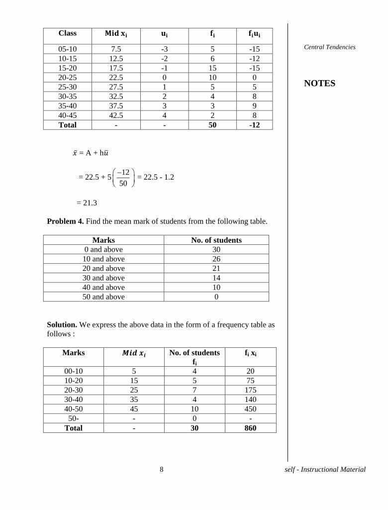
Class
05-10 7.5 -3 5 -15
10-15 12.5 -2 6 -12
15-20 17.5 -1 15 -15
20-25 22.5 0 10 0
25-30 27.5 1 5 5
30-35 32.5 2 4 8
35-40 37.5 3 3 9
40-45 42.5 4 2 8
Total - - 50 -12
= A + h
= 22.5 + 512
50
= 22.5 - 1.2
= 21.3
Problem 4. Find the mean mark of students from the following table.
Marks No. of students
0 and above 30
10 and above 26
20 and above 21
30 and above 14
40 and above 10
50 and above 0
Solution. We express the above data in the form of a frequency table as
follows :
Marks No. of students
fi
fi xi
00-10 5 4 20
10-20 15 5 75
20-30 25 7 175
30-40 35 4 140
40-50 45 10 450
50- - 0 -
Total - 30 860
Central Tendencies
NOTES
9 self - Instructional Material
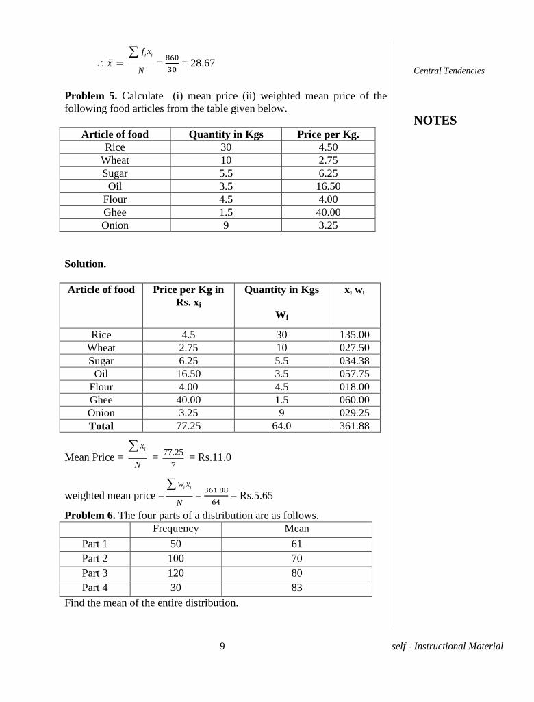
i if x
N
=
= 28.67
Problem 5. Calculate (i) mean price (ii) weighted mean price of the
following food articles from the table given below.
Article of food Quantity in Kgs Price per Kg.
Rice 30 4.50
Wheat 10 2.75
Sugar 5.5 6.25
Oil 3.5 16.50
Flour 4.5 4.00
Ghee 1.5 40.00
Onion 9 3.25
Solution.
Article of food Price per Kg in
Rs. xi
Quantity in Kgs
Wi
xi wi
Rice 4.5 30 135.00
Wheat 2.75 10 027.50
Sugar 6.25 5.5 034.38
Oil 16.50 3.5 057.75
Flour 4.00 4.5 018.00
Ghee 40.00 1.5 060.00
Onion 3.25 9 029.25
Total 77.25 64.0 361.88
Mean Price = ix
N
=
77.25
7 = Rs.11.0
weighted mean price =i iw x
N
=
= Rs.5.65
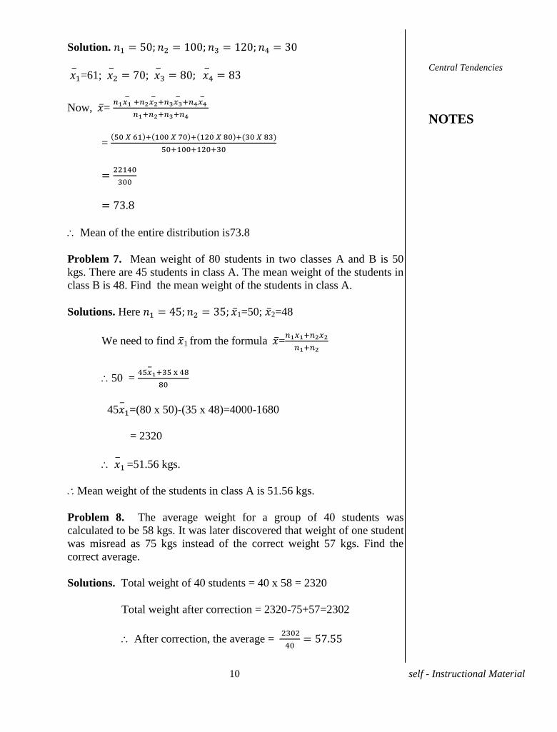
Problem 6. The four parts of a distribution are as follows.
Frequency Mean
Part 1 50 61
Part 2 100 70
Part 3 120 80
Part 4 30 83
Find the mean of the entire distribution.
Central Tendencies
NOTES
10 self - Instructional Material
Solution.
=61; ;
Now, =
=
Mean of the entire distribution is73.8
Problem 7. Mean weight of 80 students in two classes A and B is 50
kgs. There are 45 students in class A. The mean weight of the students in
class B is 48. Find the mean weight of the students in class A.
Solutions. Here 1=50; 2=48
We need to find 1 from the formula =
50 =
45
=(80 x 50)-(35 x 48)=4000-1680
= 2320
=51.56 kgs.
Mean weight of the students in class A is 51.56 kgs.
Problem 8. The average weight for a group of 40 students was
calculated to be 58 kgs. It was later discovered that weight of one student
was misread as 75 kgs instead of the correct weight 57 kgs. Find the
correct average.
Solutions. Total weight of 40 students = 40 x 58 = 2320
Total weight after correction = 2320-75+57=2302
After correction, the average =
Central Tendencies
NOTES
11 self - Instructional Material
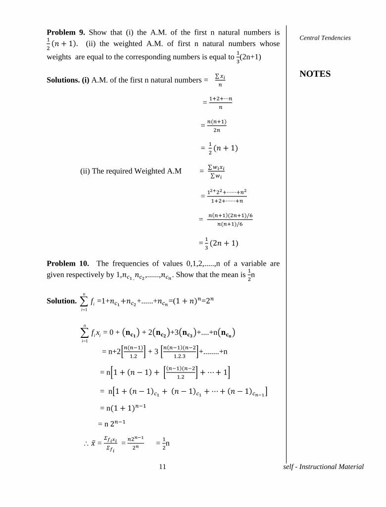
Problem 9. Show that (i) the A.M. of the first n natural numbers is
(ii) the weighted A.M. of first n natural numbers whose
weights are equal to the corresponding numbers is equal to
(2n+1)
Solutions. (i) A.M. of the first n natural numbers =
=
=
=
(ii) The required Weighted A.M =
=
=
=
)
Problem 10. The frequencies of values 0,1,2,.....,n of a variable are
given respectively by 1, ,......, . Show that the mean is
n
Solution. 1
n
i
i
f
=1+ +......+ =( =
1
n
i i
i
f x
= 0 + + 2 +3 +....+n
= n+2
+ 3
+........+n
= n
= n
= n
= n
=
=
=
n
Central Tendencies
NOTES
12 self - Instructional Material
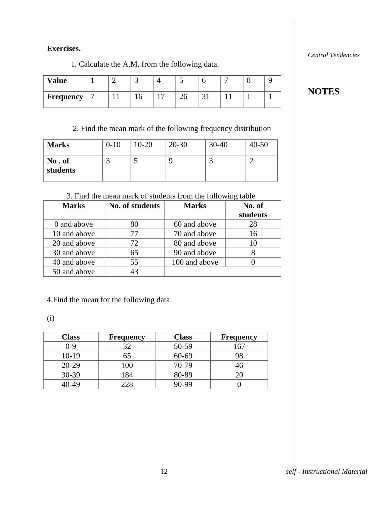
Exercises.
1. Calculate the A.M. from the following data.
Value 1 2 3 4 5 6 7 8 9
Frequency 7 11 16 17 26 31 11 1 1
2. Find the mean mark of the following frequency distribution
Marks 0-10 10-20 20-30 30-40 40-50
No . of
students
3 5 9 3 2
3. Find the mean mark of students from the following table
Marks No. of students Marks No. of
students
0 and above 80 60 and above 28
10 and above 77 70 and above 16
20 and above 72 80 and above 10
30 and above 65 90 and above 8
40 and above 55 100 and above 0
50 and above 43
4.Find the mean for the following data
(i)
Class Frequency Class Frequency
0-9 32 50-59 167
10-19 65 60-69 98
20-29 100 70-79 46
30-39 184 80-89 20
40-49 228 90-99 0
Central Tendencies
NOTES
13 self - Instructional Material
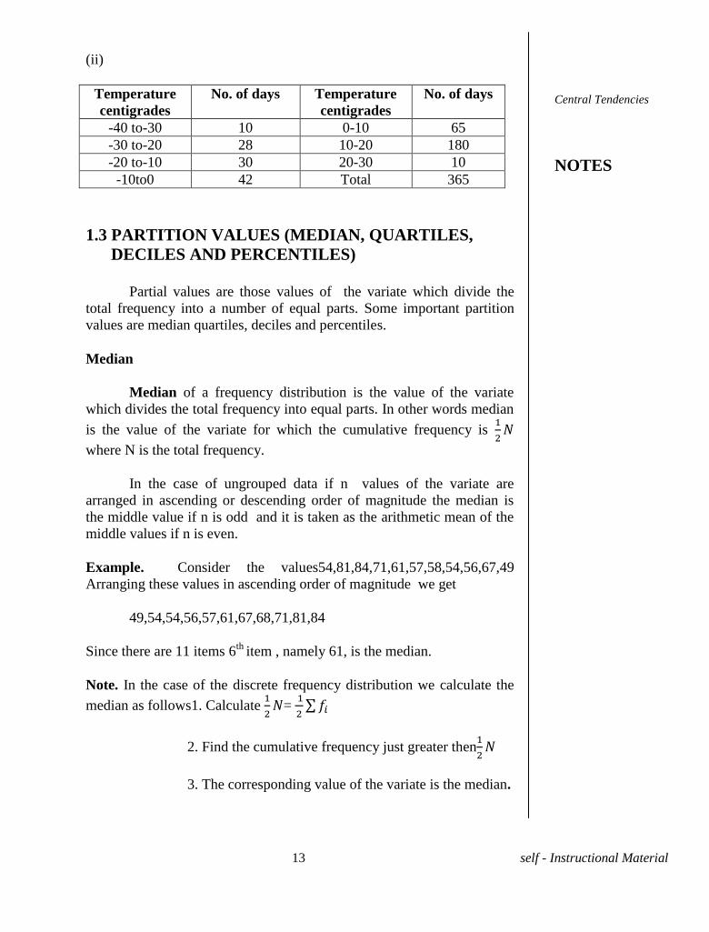
(ii)
Temperature
centigrades
No. of days Temperature
centigrades
No. of days
-40 to-30 10 0-10 65
-30 to-20 28 10-20 180
-20 to-10 30 20-30 10
-10to0 42 Total 365
1.3 PARTITION VALUES (MEDIAN, QUARTILES,
DECILES AND PERCENTILES)
Partial values are those values of the variate which divide the
total frequency into a number of equal parts. Some important partition
values are median quartiles, deciles and percentiles.
Median
Median of a frequency distribution is the value of the variate
which divides the total frequency into equal parts. In other words median
is the value of the variate for which the cumulative frequency is
where N is the total frequency.
In the case of ungrouped data if n values of the variate are
arranged in ascending or descending order of magnitude the median is
the middle value if n is odd and it is taken as the arithmetic mean of the
middle values if n is even.
Example. Consider the values54,81,84,71,61,57,58,54,56,67,49
Arranging these values in ascending order of magnitude we get
49,54,54,56,57,61,67,68,71,81,84
Since there are 11 items 6th
item , namely 61, is the median.
Note. In the case of the discrete frequency distribution we calculate the
median as follows1. Calculate
=
2. Find the cumulative frequency just greater then
3. The corresponding value of the variate is the median.
Central Tendencies
NOTES
14 self - Instructional Material
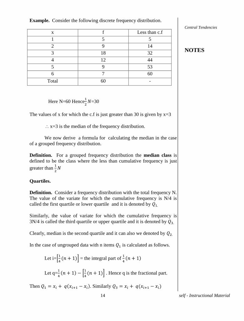
Example. Consider the following discrete frequency distribution.
x f Less than c.f
1 5 5
2 9 14
3 18 32
4 12 44
5 9 53
6 7 60
Total 60 -
Here N=60 Hence
=30
The values of x for which the c.f is just greater than 30 is given by x=3
x=3 is the median of the frequency distribution.
We now derive a formula for calculating the median in the case
of a grouped frequency distribution.
Definition. For a grouped frequency distribution the median class is
defined to be the class where the less than cumulative frequency is just
greater than
Quartiles.
Definition. Consider a frequency distribution with the total frequency N.
The value of the variate for which the cumulative frequency is N/4 is
called the first quartile or lower quartile and it is denoted by
Similarly, the value of variate for which the cumulative frequency is
3N/4 is called the third quartile or upper quartile and it is denoted by
Clearly, median is the second quartile and it can also we denoted by
In the case of ungrouped data with n items is calculated as follows.
Let i=
= the integral part of
Let q=
. Hence q is the fractional part.
Then . Similarly
Central Tendencies
NOTES
15 self - Instructional Material
where i=
and q=
-
In this case of grouped frequency distribution the quartiles are
calculated by using the formula
and
where l is the lower limit of the class in which the particular quartile lies,
is the frequency of this class, h is the width of the class and m is the
cumulative frequency of the preceeding class.
Deciles.
Consider a frequency distribution with total frequency N. The
value of the variates for which the cumulative frequencies are
9 are called deciles. The ℎ decile is denoted by Clearly
median is the fifth decile. Hence the median can also be denoted by
In the case of the ungrouped data with n items, for k=1,2,3,......,9
where i =
and q=
As before for a grouped frequency distribution we can prove that
; (i=1,2,......,9) with corresponding notations.
Percentiles
Percentiles are the values of variates for which the cumulative
frequencies are
; (i=1,2,.....,9) and the percentile is denoted by
Clearly median is percentile and hence median can alsobe denoted
by
In this case of ungrouped data with n items, for k=12,....,99
where i =
and q=
Percentile are got from the following formulae in the case of grouped
frequency distribution
; i=1,2,......,99
Central Tendencies
NOTES
16 self - Instructional Material
Solved Problems
Problems 1. Find the median and quartiles of the heights in c.m. of
eleven students given by 66,65,64,70,61,60,56,63,60,67,62
Solution. Arranging the given data in ascending order of magnitude we
get 56, 60, 60, 61, 62, 63, 64, 65, 66, 67, 70
Here n= 11. Since n is odd, median is the sixth item which is equal to 63
=size of
th
item.
= third item = 60
=
th
item = 9th
item = 66
Problem 2. Find the median and quartile marks of 10 students in
Statistics test whose marks are given as 40,90,61,68,72,43,50,84,75,33
Solution. Arranging in ascending order of magnitude we get
33,40,43,50,61,68,72,75,84,90 Here n = 10
Hence median is the average of the two middle items viz 61 and 68
Median =
(61+68) = 64.5 marks.
First quartile.
Here
-
= .75
= + .75 = 40 +.75 (43-40)=42.5
Third quartile.
= 8 and q=
=.25
= + .25 = 75 + .25 (84-75)=77.25
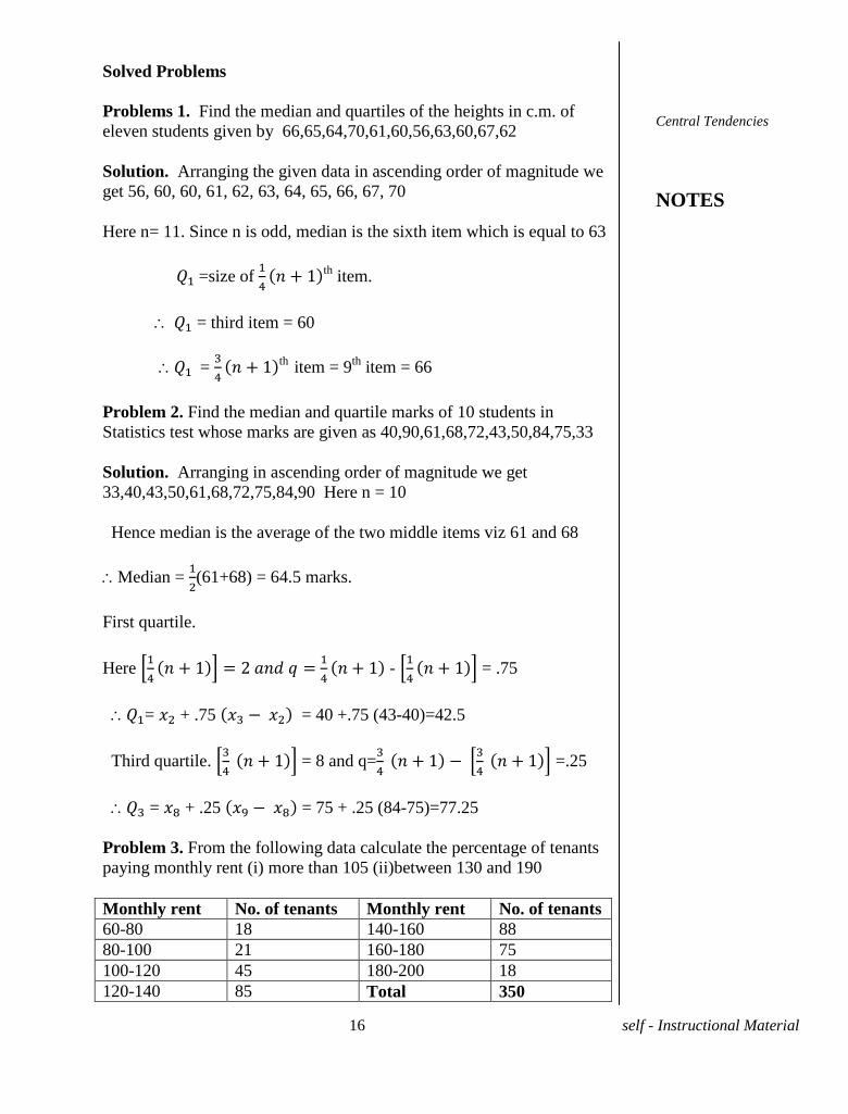
Problem 3. From the following data calculate the percentage of tenants
paying monthly rent (i) more than 105 (ii)between 130 and 190
Monthly rent No. of tenants Monthly rent No. of tenants
60-80 18 140-160 88
80-100 21 160-180 75
100-120 45 180-200 18
120-140 85 Total 350
Central Tendencies
NOTES
17 self - Instructional Material
Solution. (i) Number of tenants paying more than Rs.105 is
=
x 45+85+88+75+18
= 34+266 = 300(approximately)
Required percentage =
x 100
=85.7 (approximately)
(ii) No. of tenants paying the rent between Rs.130 and Rs.190
=
x 85+88+75+
x 18
= 42.5 + 88 +75 + 9 =215 (approximately)
Required percentage =
x 100
= 61.43
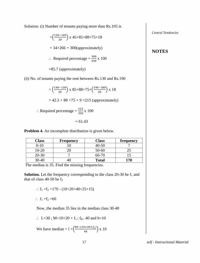
Problem 4. An incomplete distribution is given below.
Class Frequency Class frequency
0-10 10 40-50 ?
10-20 20 50-60 25
20-30 ? 60-70 15
30-40 40 Total 170
The median is 35. Find the missing frequencies.
Solution. Let the frequency corresponding to the class 20-30 be f1 and
that of class 40-50 be f2
f1 +f2 =170 - (10+20+40+25+15)
f1 +f2 =60
Now, the median 35 lies in the median class 30-40
L=30 ; M=10+20 + f1 ; fK= 40 and h=10
We have median = l +
x 10
Central Tendencies
NOTES
18 self - Instructional Material
35= 30+
(55- )
Using (2) in(1) we get
and are the missing frequencies.
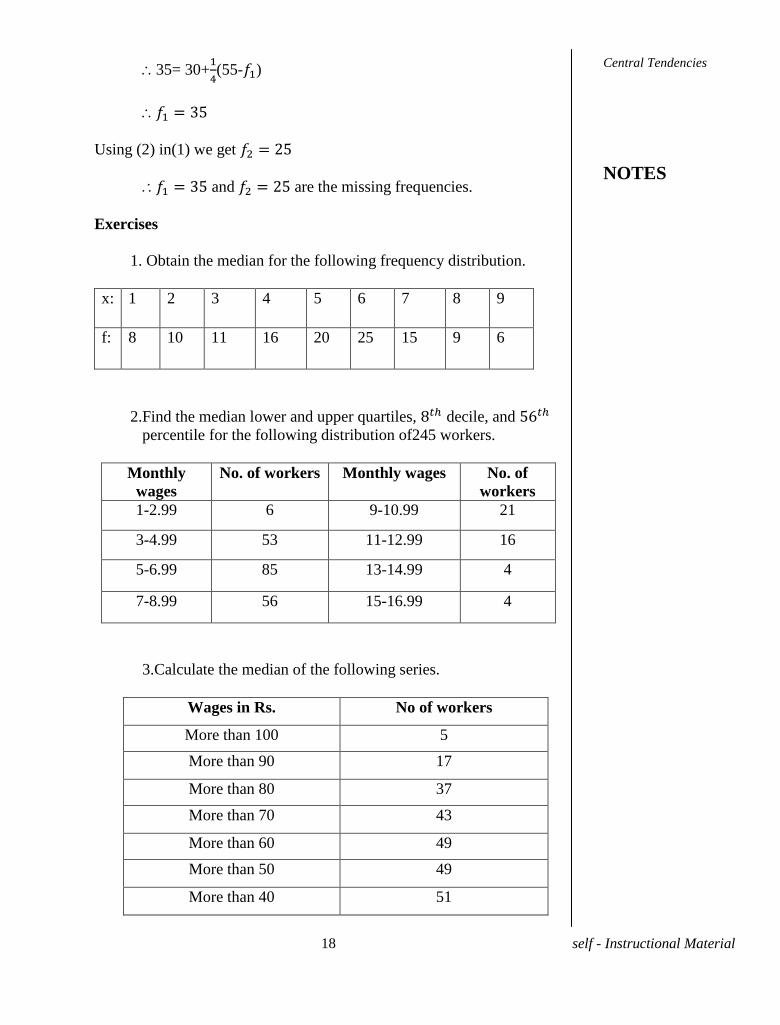
Exercises
1. Obtain the median for the following frequency distribution.
x: 1 2 3 4 5 6 7 8 9
f: 8 10 11 16 20 25 15 9 6
2.Find the median lower and upper quartiles, decile, and
percentile for the following distribution of245 workers.
Monthly
wages
No. of workers Monthly wages No. of
workers
1-2.99 6 9-10.99 21
3-4.99 53 11-12.99 16
5-6.99 85 13-14.99 4
7-8.99 56 15-16.99 4
3.Calculate the median of the following series.
Wages in Rs. No of workers
More than 100 5
More than 90 17
More than 80 37
More than 70 43
More than 60 49
More than 50 49
More than 40 51
Central Tendencies
NOTES
19 self - Instructional Material
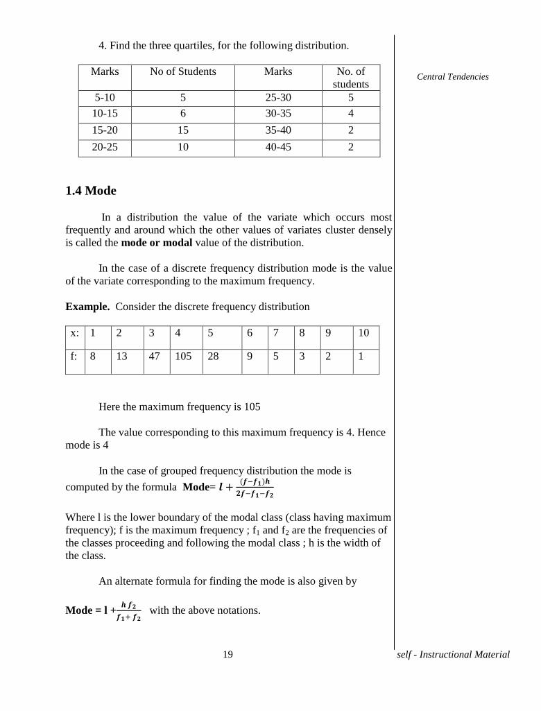
4. Find the three quartiles, for the following distribution.
Marks No of Students Marks No. of
students
5-10 5 25-30 5
10-15 6 30-35 4
15-20 15 35-40 2
20-25 10 40-45 2
1.4 Mode
In a distribution the value of the variate which occurs most
frequently and around which the other values of variates cluster densely
is called the mode or modal value of the distribution.
In the case of a discrete frequency distribution mode is the value
of the variate corresponding to the maximum frequency.
Example. Consider the discrete frequency distribution
x: 1 2 3 4 5 6 7 8 9 10
f: 8 13 47 105 28 9 5 3 2 1
Here the maximum frequency is 105
The value corresponding to this maximum frequency is 4. Hence
mode is 4
In the case of grouped frequency distribution the mode is
computed by the formula Mode=
Where l is the lower boundary of the modal class (class having maximum
frequency); f is the maximum frequency ; f1 and f2 are the frequencies of
the classes proceeding and following the modal class ; h is the width of
the class.
An alternate formula for finding the mode is also given by
Mode = l +
with the above notations.
Central Tendencies
20 self - Instructional Material
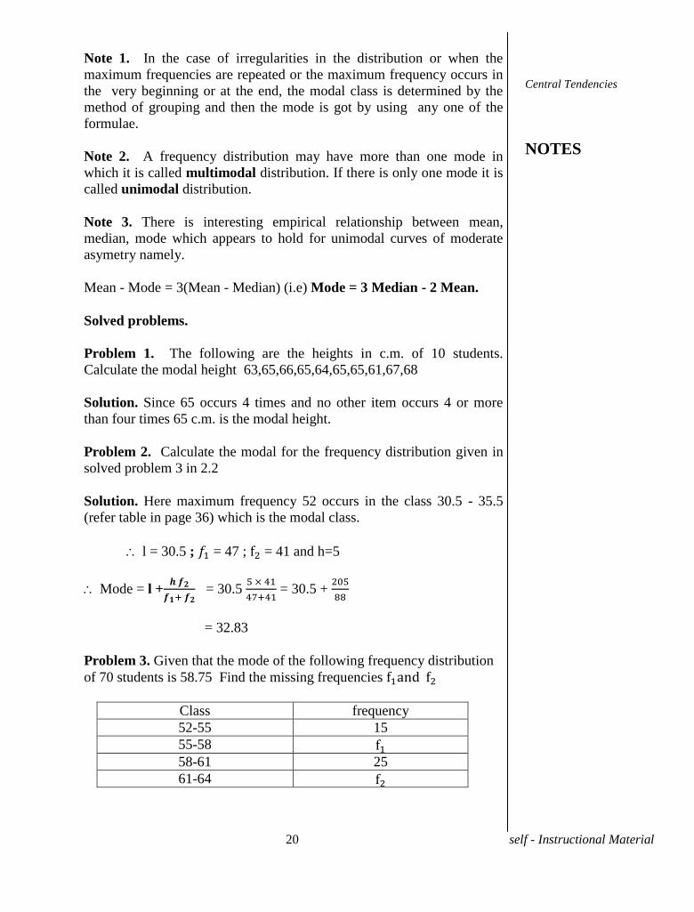
Note 1. In the case of irregularities in the distribution or when the
maximum frequencies are repeated or the maximum frequency occurs in
the very beginning or at the end, the modal class is determined by the
method of grouping and then the mode is got by using any one of the
formulae.
Note 2. A frequency distribution may have more than one mode in
which it is called multimodal distribution. If there is only one mode it is
called unimodal distribution.
Note 3. There is interesting empirical relationship between mean,
median, mode which appears to hold for unimodal curves of moderate
asymetry namely.
Mean - Mode = 3(Mean - Median) (i.e) Mode = 3 Median - 2 Mean.
Solved problems.
Problem 1. The following are the heights in c.m. of 10 students.
Calculate the modal height 63,65,66,65,64,65,65,61,67,68
Solution. Since 65 occurs 4 times and no other item occurs 4 or more
than four times 65 c.m. is the modal height.
Problem 2. Calculate the modal for the frequency distribution given in
solved problem 3 in 2.2
Solution. Here maximum frequency 52 occurs in the class 30.5 - 35.5
(refer table in page 36) which is the modal class.
l = 30.5 ; = 47 ; = 41 and h=5
Mode = l +
= 30.5
= 30.5 +
= 32.83
Problem 3. Given that the mode of the following frequency distribution
of 70 students is 58.75 Find the missing frequencies
Class frequency
52-55 15
55-58
58-61 25
61-64
Central Tendencies
NOTES
21 self - Instructional Material
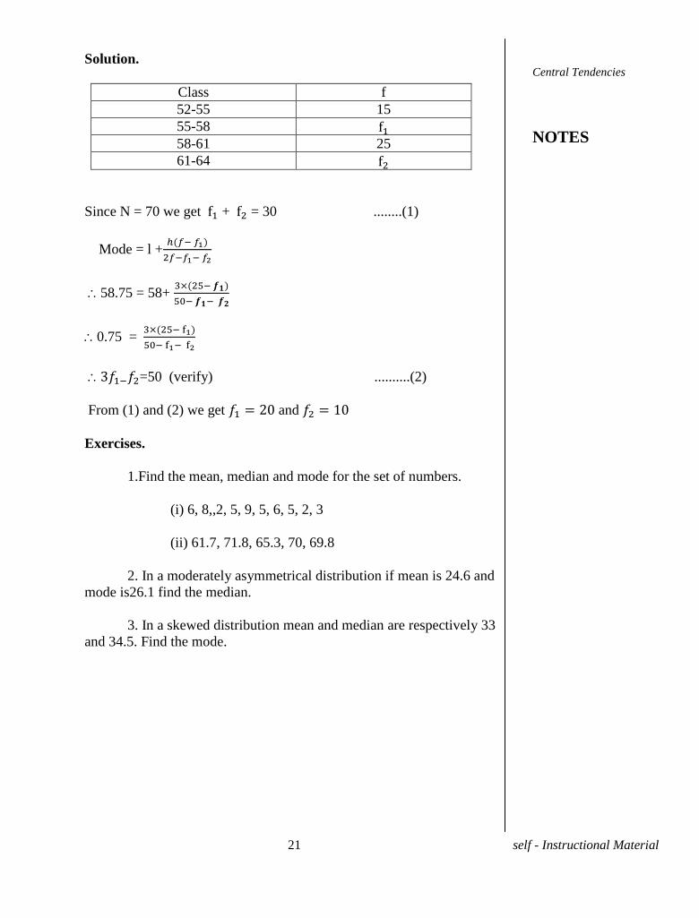
Solution.
Class f
52-55 15
55-58
58-61 25
61-64
Since N = 70 we get + = 30 ........(1)
Mode = l +
58.75 = 58+
0.75 =
=50 (verify) ..........(2)
From (1) and (2) we get and
Exercises.
1.Find the mean, median and mode for the set of numbers.
(i) 6, 8,,2, 5, 9, 5, 6, 5, 2, 3
(ii) 61.7, 71.8, 65.3, 70, 69.8
2. In a moderately asymmetrical distribution if mean is 24.6 and
mode is26.1 find the median.
3. In a skewed distribution mean and median are respectively 33
and 34.5. Find the mode.
Central Tendencies
NOTES
22 self - Instructional Material
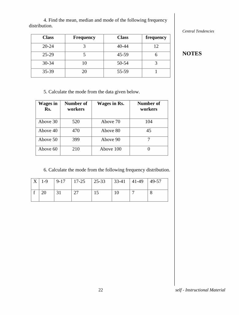
4. Find the mean, median and mode of the following frequency
distribution.
Class Frequency Class frequency
20-24 3 40-44 12
25-29 5 45-59 6
30-34 10 50-54 3
35-39 20 55-59 1
5. Calculate the mode from the data given below.
Wages in
Rs.
Number of
workers
Wages in Rs. Number of
workers
Above 30 520 Above 70 104
Above 40 470 Above 80 45
Above 50 399 Above 90 7
Above 60 210 Above 100 0
6. Calculate the mode from the following frequency distribution.
X 1-9 9-17 17-25 25-33 33-41 41-49 49-57
f 20 31 27 15 10 7 8
Central Tendencies
NOTES
23 self - Instructional Material
UNIT-II GEOMETRIC MEAN AND
HARMONIC MEAN
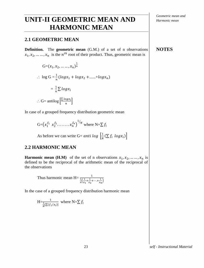
2.1 GEOMETRIC MEAN
Definition. The geometric mean (G.M.) of a set of n observations
is the root of their product. Thus, geometric mean is
G=
log G =
......+
=
G=
In case of a grouped frequency distribution geometric mean
G=
where N=
As before we can write G=
2.2 HARMONIC MEAN
Harmonic mean (H.M) of the set of n observations is
defined to be the reciprocal of the arithmetic mean of the reciprocal of
the observations
Thus harmonic mean H=
In the case of a grouped frequency distribution harmonic mean
H=
where N=
Geometric mean and
Harmonic mean
NOTES
24 self - Instructional Material
Solved Problems.
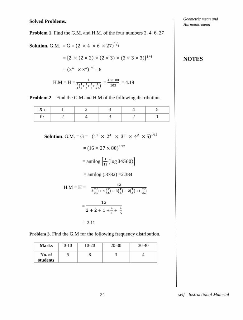
Problem 1. Find the G.M. and H.M. of the four numbers 2, 4, 6, 27
Solution. G.M. = G =
=
= 1/4 = 6
H.M = H =
=
= 4.19
Problem 2. Find the G.M and H.M of the following distribution.
X : 1 2 3 4 5
f : 2 4 3 2 1
Solution. G.M. = G = 1/12
= (16 1/12
= antilog
= antilog (.3782) =2.384
H.M = H =
=
= 2.11
Problem 3. Find the G.M for the following frequency distribution.
Marks 0-10 10-20 20-30 30-40
No. of
students
5 8 3 4
Geometric mean and
Harmonic mean
NOTES
25 self - Instructional Material
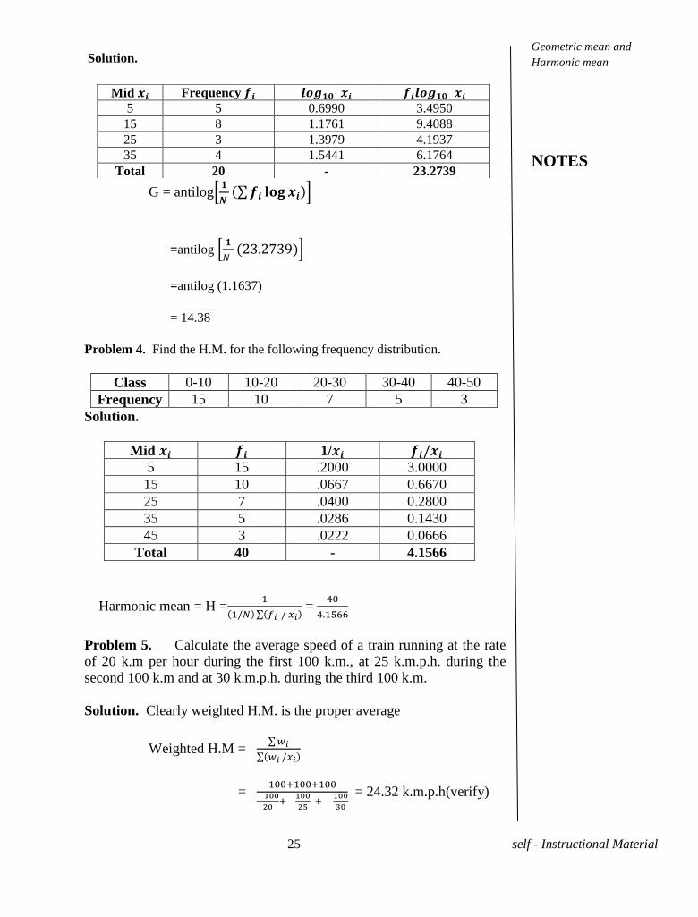
Solution.
G = antilog
=antilog
9
=antilog (1.1637)
= 14.38
Problem 4. Find the H.M. for the following frequency distribution.
Class 0-10 10-20 20-30 30-40 40-50
Frequency 15 10 7 5 3
Solution.
Mid 1/ 5 15 .2000 3.0000
15 10 .0667 0.6670
25 7 .0400 0.2800
35 5 .0286 0.1430
45 3 .0222 0.0666
Total 40 - 4.1566
Harmonic mean = H =
=
Problem 5. Calculate the average speed of a train running at the rate
of 20 k.m per hour during the first 100 k.m., at 25 k.m.p.h. during the
second 100 k.m and at 30 k.m.p.h. during the third 100 k.m.
Solution. Clearly weighted H.M. is the proper average
Weighted H.M =
=
= 24.32 k.m.p.h(verify)
Mid Frequency 5 5 0.6990 3.4950
15 8 1.1761 9.4088
25 3 1.3979 4.1937
35 4 1.5441 6.1764
Total 20 - 23.2739
Geometric mean and
Harmonic mean
NOTES
26 self - Instructional Material
Exercises
1. Calculate A.M., G.M. and H.M. of the following observations
and show that A.M > G.M > H.M. 32,35,36,37,39,41,43
2. Calculate the H.M of the following series of monthly
expenditure in Rs.of a batch of students 125,130,75,10,45,0.5,0.4, 500,15
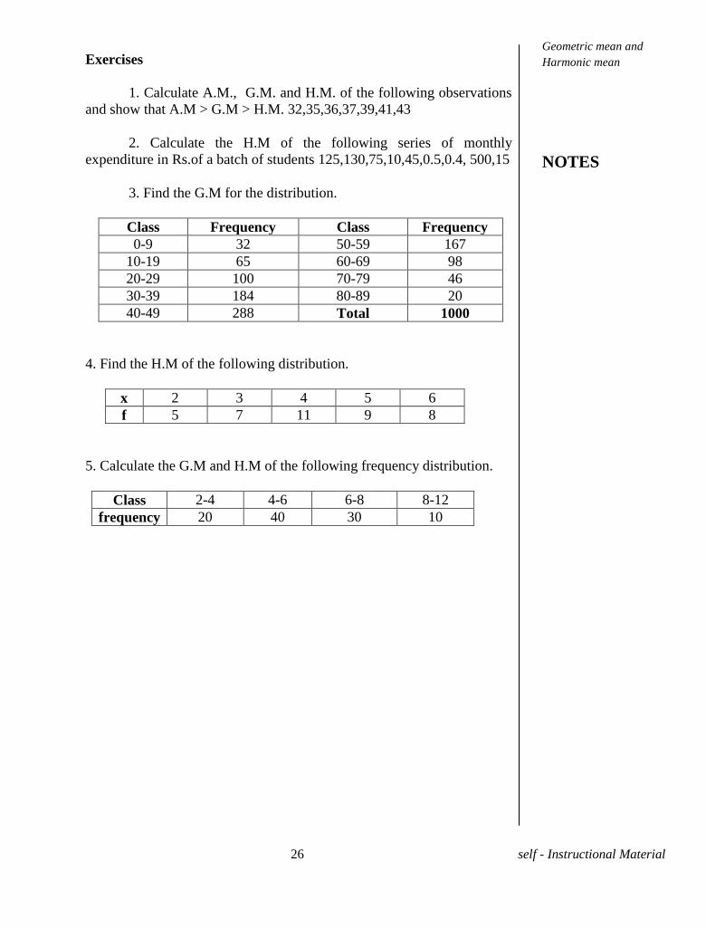
3. Find the G.M for the distribution.
Class Frequency Class Frequency
0-9 32 50-59 167
10-19 65 60-69 98
20-29 100 70-79 46
30-39 184 80-89 20
40-49 288 Total 1000
4. Find the H.M of the following distribution.
x 2 3 4 5 6
f 5 7 11 9 8
5. Calculate the G.M and H.M of the following frequency distribution.
Class 2-4 4-6 6-8 8-12
frequency 20 40 30 10
Geometric mean and
Harmonic mean
NOTES
27 self - Instructional Material
UNIT-III MEASURES OF DISPERSION
3.1 INTRODUCTION
You have learnt various measures of central tendency. Measures of
central tendency help us to represent the entire mass of the data by a
single value. Can the central tendency describe the data fully and
adequately? In order to understand it, let us consider an example.
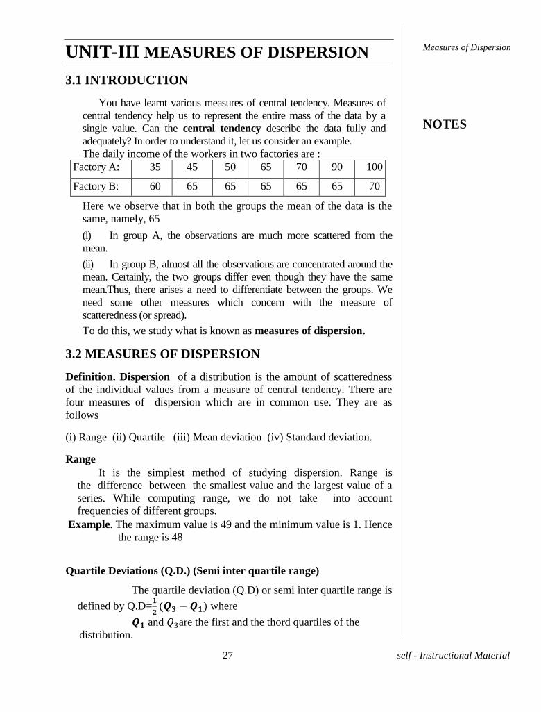
The daily income of the workers in two factories are :
Factory A: 35 45 50 65 70 90 100
Factory B: 60 65 65 65 65 65 70
Here we observe that in both the groups the mean of the data is the
same, namely, 65
(i) In group A, the observations are much more scattered from the
mean.
(ii) In group B, almost all the observations are concentrated around the
mean. Certainly, the two groups differ even though they have the same
mean.Thus, there arises a need to differentiate between the groups. We
need some other measures which concern with the measure of
scatteredness (or spread).
To do this, we study what is known as measures of dispersion.
3.2 MEASURES OF DISPERSION
Definition. Dispersion of a distribution is the amount of scatteredness
of the individual values from a measure of central tendency. There are
four measures of dispersion which are in common use. They are as
follows
(i) Range (ii) Quartile (iii) Mean deviation (iv) Standard deviation.
Range
It is the simplest method of studying dispersion. Range is
the difference between the smallest value and the largest value of a
series. While computing range, we do not take into account
frequencies of different groups.
Example. The maximum value is 49 and the minimum value is 1. Hence
the range is 48
Quartile Deviations (Q.D.) (Semi inter quartile range)
The quartile deviation (Q.D) or semi inter quartile range is
defined by Q.D=
where
and are the first and the thord quartiles of the
distribution.
Measures of Dispersion
NOTES
28 self - Instructional Material
Example. =17 and
Hence Q.D =
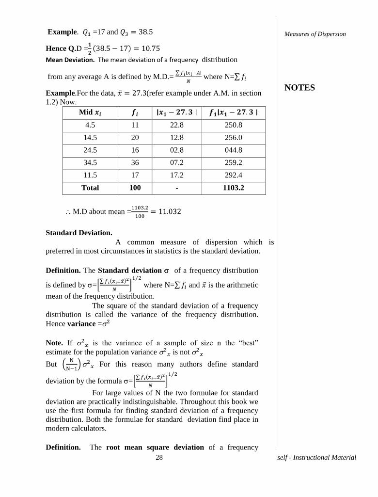
Mean Deviation. The mean deviation of a frequency distribution
from any average A is defined by M.D.=
where N=
Example.For the data, (refer example under A.M. in section
1.2) Now.
Mid
4.5 11 22.8 250.8
14.5 20 12.8 256.0
24.5 16 02.8 044.8
34.5 36 07.2 259.2
11.5 17 17.2 292.4
Total 100 - 1103.2
M.D about mean =
Standard Deviation.
A common measure of dispersion which is
preferred in most circumstances in statistics is the standard deviation.
Definition. The Standard deviation of a frequency distribution
is defined by =
where N= and is the arithmetic
mean of the frequency distribution.
The square of the standard deviation of a frequency
distribution is called the variance of the frequency distribution.
Hence variance =
Note. If s he v r ce f s mp e f s ze he “bes ”
estimate for the population variance is not
But
For this reason many authors define standard
deviation by the formula =
For large values of N the two formulae for standard
deviation are practically indistinguishable. Throughout this book we
use the first formula for finding standard deviation of a frequency
distribution. Both the formulae for standard deviation find place in
modern calculators.
Definition. The root mean square deviation of a frequency
Measures of Dispersion
NOTES
29 self - Instructional Material
distribution is defined to be s=
where A is any arbitrary origin and is called the mean square
deviation.
Definition. Coefficient of variation of a frequency distribution is
defined to be C.V =
x 100
For comparing the variability of two sets of
observations of a frequency distribution we calculate the C.V for
each of the set of frequency distribution. The set having smaller C.V
is said to be more consistent than the other.
Example1 . Consider the numbers 1, 2, 3, 4, 5, 5, 7
Their arithmetic mean =4
Now, =28.(verify)
=
=
=2
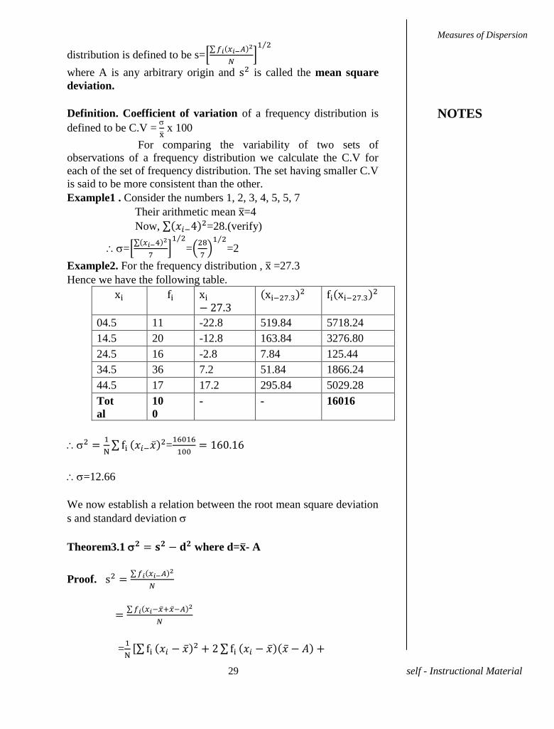
Example2. For the frequency distribution , =27.3
Hence we have the following table.
04.5 11 -22.8 519.84 5718.24
14.5 20 -12.8 163.84 3276.80
24.5 16 -2.8 7.84 125.44
34.5 36 7.2 51.84 1866.24
44.5 17 17.2 295.84 5029.28
Tot
al
10
0
- - 16016
=
=12.66
We now establish a relation between the root mean square deviation
s and standard deviation
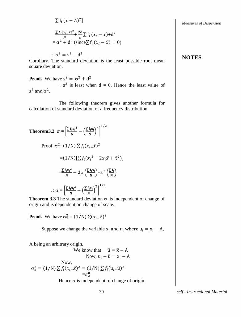
Theorem3.1 where d= - A
Proof.
=
Measures of Dispersion
NOTES
30 self - Instructional Material
=
+
+
= (since )
Corollary. The standard deviation is the least possible root mean
square deviation.
Proof. We have
is least when d = 0. Hence the least value of
The following theorem gives another formula for
calculation of standard deviation of a frequency distribution.
Theorem3.2 =
Proof. =
=
=
+
=
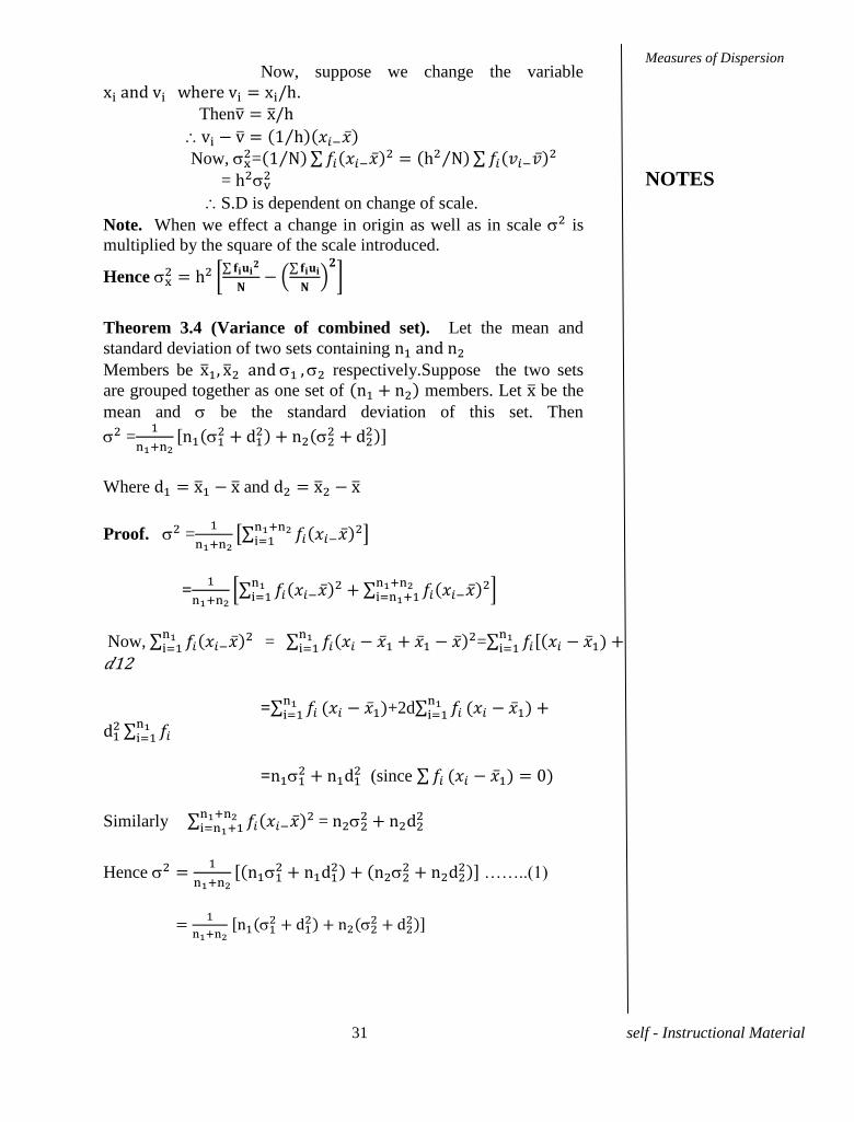
Theorem 3.3 The standard deviation is independent of change of
origin and is dependent on change of scale.
Proof. We have =
Suppose we change the variable ,
A being an arbitrary origin.
We know that
Now,
Now,
=
Hence is independent of change of origin.
Measures of Dispersion
NOTES
31 self - Instructional Material
Now, suppose we change the variable
.
Then
Now,
=
=
S.D is dependent on change of scale.
Note. When we effect a change in origin as well as in scale is
multiplied by the square of the scale introduced.
Hence
Theorem 3.4 (Variance of combined set). Let the mean and
standard deviation of two sets containing
Members be respectively.Suppose the two sets
are grouped together as one set of members. Let be the
mean and be the standard deviation of this set. Then
=
Where and
Proof. =
=
Now,
= =
12
= +2d
=
(since
Similarly
=
Hence
……..(1)
Measures of Dispersion
NOTES
32 self - Instructional Material
Solved Problems.
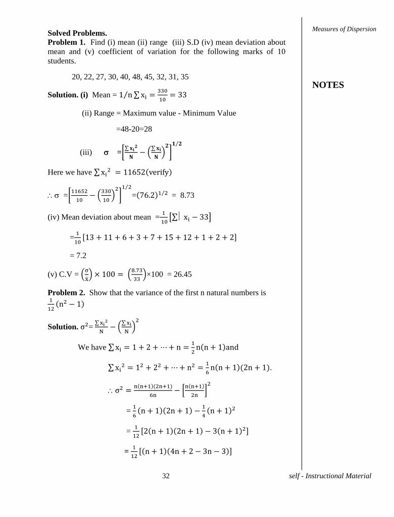
Problem 1. Find (i) mean (ii) range (iii) S.D (iv) mean deviation about
mean and (v) coefficient of variation for the following marks of 10
students.
20, 22, 27, 30, 40, 48, 45, 32, 31, 35
Solution. (i) Mean =
(ii) Range = Maximum value - Minimum Value
=48-20=28
(iii) =
Here we have
=
= = 8.73
(iv) Mean deviation about mean =
=
= 7.2
(v) C.V =
×100 = 26.45
Problem 2. Show that the variance of the first n natural numbers is
Solution. =
We have
.
=
=
=
Measures of Dispersion
NOTES
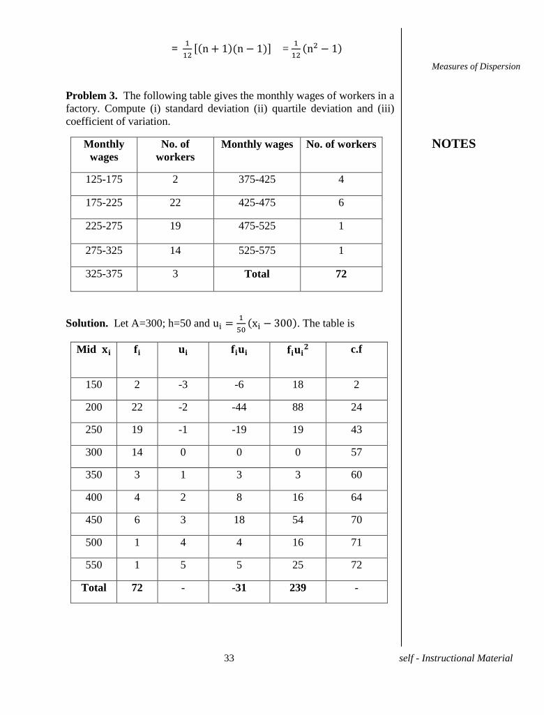
33 self - Instructional Material
=
=
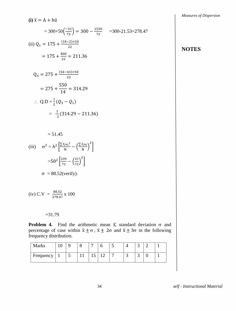
Problem 3. The following table gives the monthly wages of workers in a
factory. Compute (i) standard deviation (ii) quartile deviation and (iii)
coefficient of variation.
Monthly
wages
No. of
workers
Monthly wages No. of workers
125-175 2 375-425 4
175-225 22 425-475 6
225-275 19 475-525 1
275-325 14 525-575 1
325-375 3 Total 72
Solution. Let A=300; h=50 and
. The table is
Mid
c.f
150 2 -3 -6 18 2
200 22 -2 -44 88 24
250 19 -1 -19 19 43
300 14 0 0 0 57
350 3 1 3 3 60
400 4 2 8 16 64
450 6 3 18 54 70
500 1 4 4 16 71
550 1 5 5 25 72
Total 72 - -31 239 -
Measures of Dispersion
NOTES
34 self - Instructional Material
(i)
= 300+50
=300-21.53=278.47
(ii)
9
Q.D =
=
9
= 51.45
(iii) = ℎ
=
= 88.52(verify).
(iv) C.V =
x 100
=31.79
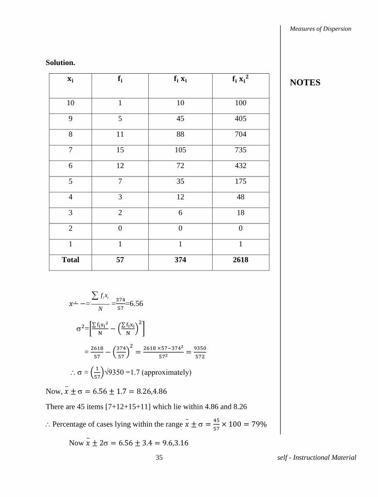
Problem 4. Find the arithmetic mean standard deviation and
percentage of case within and in the following
frequency distribution.
Marks 10 9 8 7 6 5 4 3 2 1
Frequency 1 5 11 15 12 7 3 3 0 1
Measures of Dispersion
NOTES
35 self - Instructional Material
Solution.
10 1 10 100
9 5 45 405
8 11 88 704
7 15 105 735
6 12 72 432
5 7 35 175
4 3 12 48
3 2 6 18
2 0 0 0
1 1 1 1
Total 57 374 2618
=i if x
N
=
=6.56
=
=
=
√9350 =1.7 ( ppr x m e y)
Now,
There are 45 items [7+12+15+11] which lie within 4.86 and 8.26
Percentage of cases lying within the range
9
Now 9
Measures of Dispersion
NOTES
36 self - Instructional Material
There are only 53 items [3+7+12+15+11+5] which is within 3.16
and 9.96
Percentage of items lying within the range
=
=93%
Similarly the percentage of items lying within the range
9
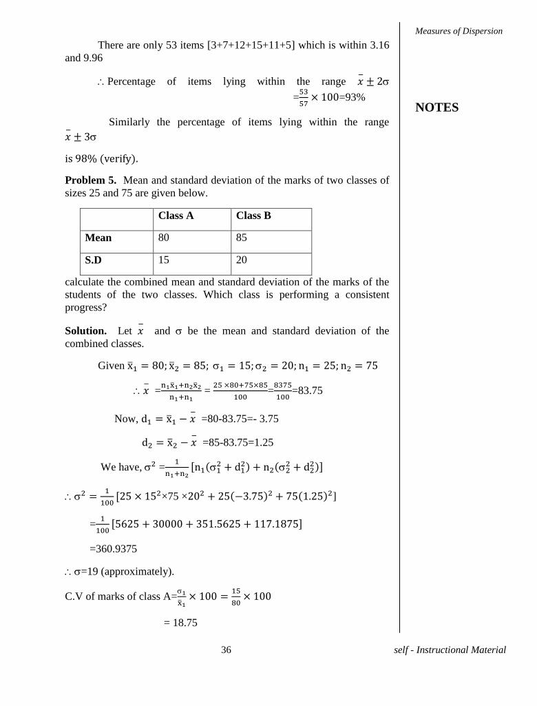
Problem 5. Mean and standard deviation of the marks of two classes of
sizes 25 and 75 are given below.
Class A Class B
Mean 80 85
S.D 15 20
calculate the combined mean and standard deviation of the marks of the
students of the two classes. Which class is performing a consistent
progress?
Solution. Let
and be the mean and standard deviation of the
combined classes.
Given
=
=
=
=83.75
Now,
=80-83.75=- 3.75
=85-83.75=1.25
We have, =
×75 × ]
=
=360.9375
=19 (approximately).
C.V of marks of class A=
= 18.75
Measures of Dispersion
NOTES
37 self - Instructional Material
C.V of marks of class B=
= 23.53
Since the C.V of marks of class A is smaller than that of class B , class A
is performing consistent progress.
Problem 6. Prove that for any discrete distribution standard deviation is
not less than the mean deviation from mean.
Solution. Let m=mean deviation from mean.
m=
We have to prove not less than m.
(i.e) to prove that
Now, ≥
where
which is true.
Hence the result.
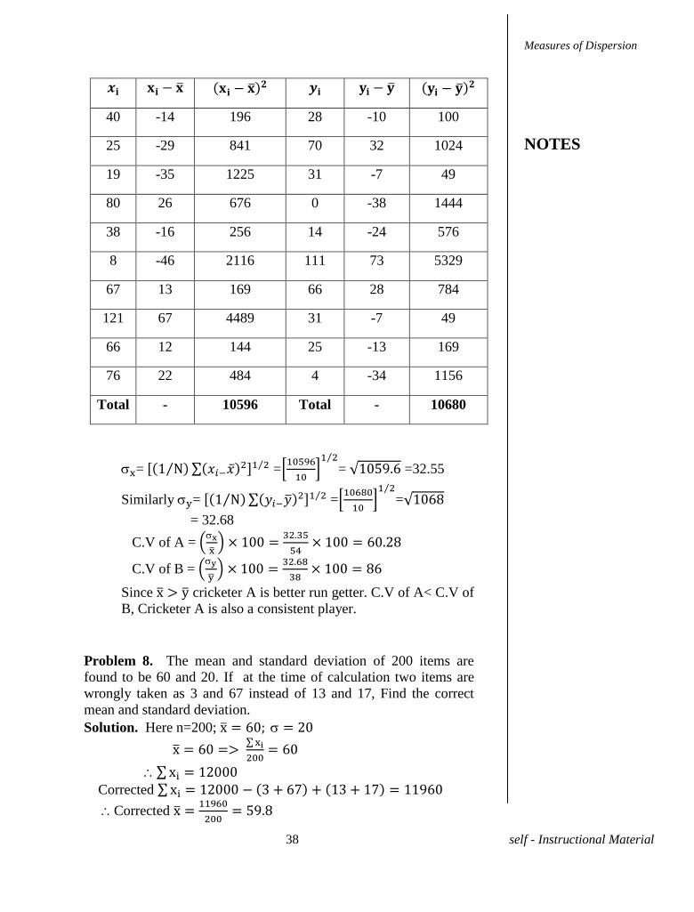
Problem 7. The scores of two cricketers A and B in 10 innings are given
below. Find who is a better run getter and who is more consistent player.
A scores 40 25 19 80 38 8 67 121 66 76
B scores 28 70 31 0 14 111 66 31 25 4
Solution. For cricketer A: =
For cricketer B: =
Measures of Dispersion
NOTES
38 self - Instructional Material
40 -14 196 28 -10 100
25 -29 841 70 32 1024
19 -35 1225 31 -7 49
80 26 676 0 -38 1444
38 -16 256 14 -24 576
8 -46 2116 111 73 5329
67 13 169 66 28 784
121 67 4489 31 -7 49
66 12 144 25 -13 169
76 22 484 4 -34 1156
Total - 10596 Total - 10680
= =
= 9 =32.55
Similarly = =
=
= 32.68
C.V of A =
C.V of B =
Since cricketer A is better run getter. C.V of A< C.V of
B, Cricketer A is also a consistent player.
Problem 8. The mean and standard deviation of 200 items are
found to be 60 and 20. If at the time of calculation two items are
wrongly taken as 3 and 67 instead of 13 and 17, Find the correct
mean and standard deviation.
Solution. Here n=200;
Corrected 9
Corrected
9
Measures of Dispersion
NOTES
39 self - Instructional Material
=
. Hence
After correction
9 9
Corrected
9
=20.09
Problem9. Find (i) the mean deviation from the mean (ii) variance of
the arithmetic progression a, a+d, a+2d, ......, a+2nd.
Solution. There are 2n +1 terms in the A.P
=
= a+nd
(i) Mean deviation from mean =
=
=
(iii) Variance
=
=
=
Exercises.
1. Calculate mean, S.D and C.V of the marks obtained by 20
students in an examination.
62 85 73 81 74 58 66 72 54 84
65 50 83 62 85 52 80 86 71 75
2.Calculate the standard deviation from the following data of
income of 10 employees of a firm.
100 120 140 120 180 175 185 130 200 150
3. Prepare a frequency table from the following passage taking
consonants and vowels in each word as two variable x and y. Find
Measures of Dispersion
NOTES
40 self - Instructional Material
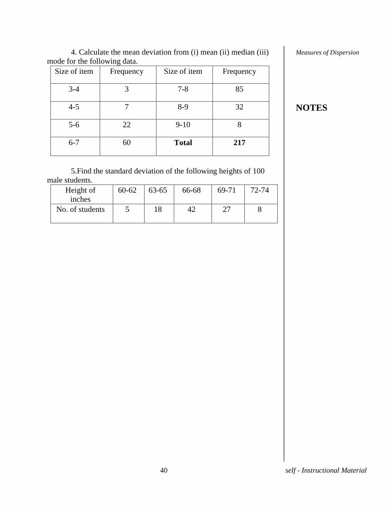
4. Calculate the mean deviation from (i) mean (ii) median (iii)
mode for the following data.
Size of item Frequency Size of item Frequency
3-4 3 7-8 85
4-5 7 8-9 32
5-6 22 9-10 8
6-7 60 Total 217
5.Find the standard deviation of the following heights of 100
male students.
Height of
inches
60-62 63-65 66-68 69-71 72-74
No. of students 5 18 42 27 8
Measures of Dispersion
NOTES
41 self - Instructional Material
UNIT-IV MOMENTS SKEWNESS AND
KURTOSIS
4.1 INTRODUCTION
In previous chapters we have introduced certain measures of
central tendencies and measures of dispersion with the aim of finding a "
few statistical constants" that represent the entire data. In this chapter we
introduce some more statistical constants known as moments.
4.2.MOMENTS
Definition. The rth
moment about any point A, denoted by µr of a
frequency distribution (fi/xi) is defined by µr =
When A = 0 We get µr ==
which is the r
th moment about the
origin.
The rth
moment about the arithmetic mean of a frequency
distribution is given by µr =
µr is also called the rth
central moment.
Note 1. The first moment about origin coincides with the A.M of the
frequency distribution and µ2 is nothing but the variance of the frequency
distribution.
Note 2. µ1 =
0 ;
Note 3. µ1 =
=
= - A
= A + µ1
We now establish a relation between µr' and µr
Theorem 4.1
µr= -
+ µr-1(
)2
.......... +(-1) r-1
(r-1)( )
r
Proof. µr =
Moments Skewness and
Kurtosis
NOTES
42 self - Instructional Material
= where d= -A
= -
rc d fi xi A µ1+ ) fi]
=
- d
+ .-......... +(-1)
r-1 (
) +
=
-
+ µr-1(
)2
.......... +(-1) r-1
(r-1)( )
r
Note. Putting r = 2, 3, 4 in the above theorem we have
(i)
(ii)
(iii)
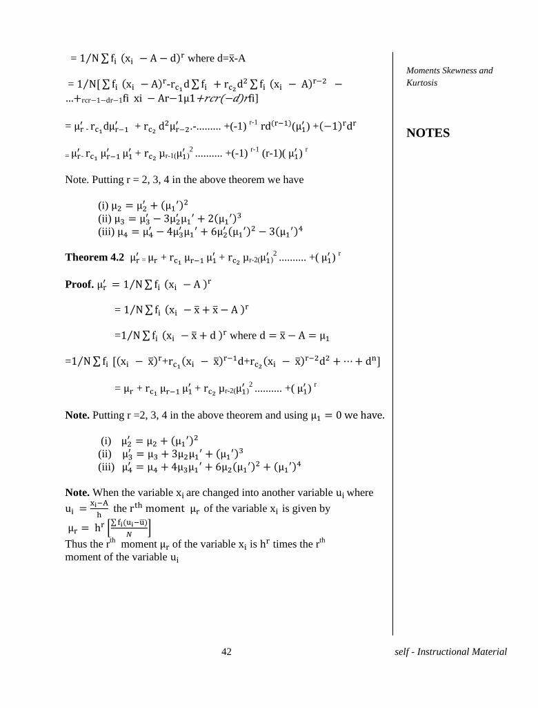
Theorem 4.2
= +
+ µr-2(
)2
.......... +( )
r
Proof.
=
= where
= +
+
= +
+ µr-2(
)2
.......... +( )
r
Note. Putting r =2, 3, 4 in the above theorem and using
(i)
(ii)
(iii)
Note. When the variable are changed into another variable where
the
of the variable is given by
Thus the rth
moment of the variable is times the rth
moment of the variable
Moments Skewness and
Kurtosis
NOTES
43 self - Instructional Material
Definition. Karl Pearson's and coefficients are defined as follows.
=
and =
= and =
The above four coefficients depends upon the first four central
moments. They are pure numbers independent of units in which the
variable is expresses. Also their values are not affected by change of
origin and scale. These constants are used in section 4.3 in the study of
skewness and kurtosis.
4.3 SKEWNESS AND KURTOSIS
If the values of a variable are distributed symmetrically about
the mean which is taken as the origin then for every positive value of x - there corresponds a negative equal value. Hence when these values are
clubed they retain their signs and cancel on addition.
µ3 =
3 = 0 . Hence =
= 0
Thus in the case of symmetrical distribution fails to be
symmetrical (asymmetrical) then we say that it is skewed distribution.,
Thus skewness means lack of symmetry. From the above discussion we
see that can be taken as a measure of skewness. We say that a
frequency distribution has positive skewness if >0 and negative
skewness if < 0
For a symmetric distribution the mean ,median and mode
coincide. Hence for an asymmetrical distribution the distance between
the median and mean may be used as measures of skewness.
Mean -Mode and Mean - Median may be taken as measures of
skewness.
To make these measures free from units of measurements so that
comparison with other distribution may be possible we divide them by a
suitable measure of dispersion and obtain the following coefficients of
skewness.
(i) Karl Person's coefficient of skewness.
-
are called Karl Pearson's coefficients
of skewness.
Moments Skewness and
Kurtosis
NOTES
44 self - Instructional Material
(ii)Bowley's coefficient of skewness is given by
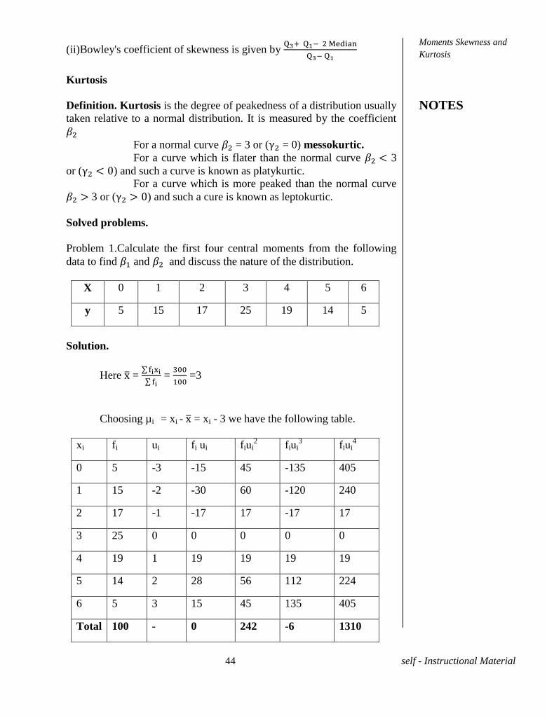
Kurtosis
Definition. Kurtosis is the degree of peakedness of a distribution usually
taken relative to a normal distribution. It is measured by the coefficient
For a normal curve = 3 or ( = 0) messokurtic.
For a curve which is flater than the normal curve 3
or ( ) and such a curve is known as platykurtic.
For a curve which is more peaked than the normal curve
3 or ( ) and such a cure is known as leptokurtic.
Solved problems.
Problem 1.Calculate the first four central moments from the following
data to find and and discuss the nature of the distribution.
X 0 1 2 3 4 5 6
y 5 15 17 25 19 14 5
Solution.
Here =
=
=3
Choosing µi = xi - = xi - 3 we have the following table.
xi fi ui fi ui fiui2
fiui3 fiui
4
0 5 -3 -15 45 -135 405
1 15 -2 -30 60 -120 240
2 17 -1 -17 17 -17 17
3 25 0 0 0 0 0
4 19 1 19 19 19 19
5 14 2 28 56 112 224
6 5 3 15 45 135 405
Total 100 - 0 242 -6 1310
Moments Skewness and
Kurtosis
NOTES
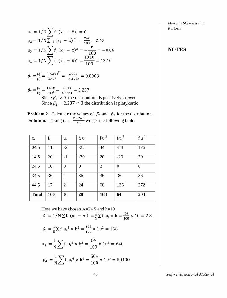
45 self - Instructional Material
=
=
=
Since the distribution is positively skewed.
Since the distribution is platykurtic.
Problem 2. Calculate the values of and for the distribution.
Solution. Taking
we get the following table.
xi fi ui fi ui fiui2
fiui3 fiui
4
04.5 11 -2 -22 44 -88 176
14.5 20 -1 -20 20 -20 20
24.5 16 0 0 2 0 0
34.5 36 1 36 36 36 36
44.5 17 2 24 68 136 272
Total 100 0 28 168 64 504
Here we have chosen A=24.5 and h=10
Moments Skewness and
Kurtosis
NOTES
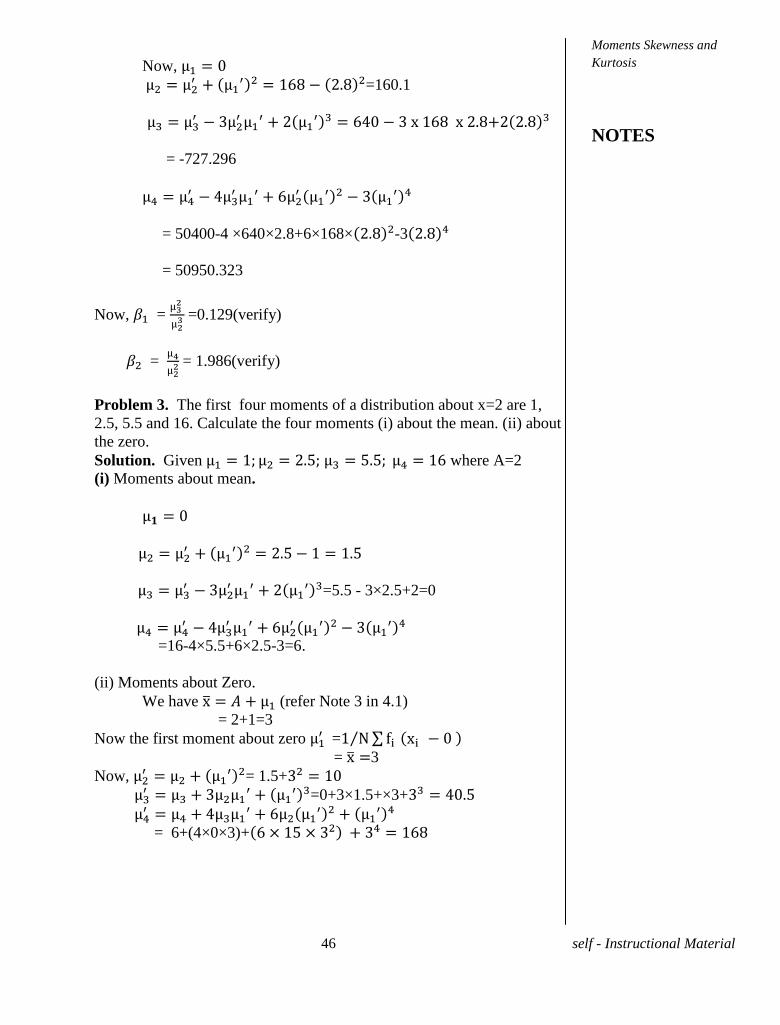
46 self - Instructional Material
Now,
=160.1
= -727.296
= 50400-4 ×640×2.8+6×168× -3
= 50950.323
Now, =
=0.129(verify)
=
= 1.986(verify)
Problem 3. The first four moments of a distribution about x=2 are 1,
2.5, 5.5 and 16. Calculate the four moments (i) about the mean. (ii) about
the zero.
Solution. Given where A=2
(i) Moments about mean.
=5.5 - 3×2.5+2=0
=16-4×5.5+6×2.5-3=6.
(ii) Moments about Zero.
We have (refer Note 3 in 4.1)
= 2+1=3
Now the first moment about zero =
= 3
Now,
= 1.5+
=0+3×1.5+×3+
= 6+(4×0×3)+
Moments Skewness and
Kurtosis
NOTES
47 self - Instructional Material
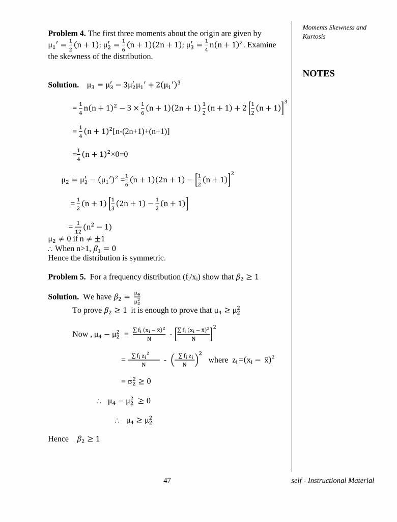
Problem 4. The first three moments about the origin are given by
. Examine
the skewness of the distribution.
Solution.
=
=
[n-(2n+1)+(n+1)]
=
×0=0
=
=
=
When n>1,
Hence the distribution is symmetric.
Problem 5. For a frequency distribution (fi/xi) show that
Solution. We have
To prove it is enough to prove that
Now , =
-
=
-
where zi = 2
=
Hence
Moments Skewness and
Kurtosis
NOTES
48 self - Instructional Material
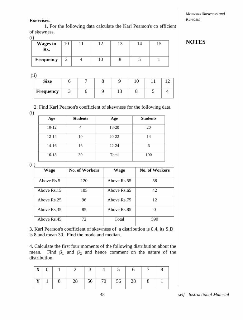
Exercises.
1. For the following data calculate the Karl Pearson's co efficient
of skewness.
(i)
Wages in
Rs.
10 11 12 13 14 15
Frequency 2 4 10 8 5 1
(ii)
Size 6 7 8 9 10 11 12
Frequency 3 6 9 13 8 5 4
2. Find Karl Pearson's coefficient of skewness for the following data.
(i) Age Students Age Students
10-12 4 18-20 20
12-14 10 20-22 14
14-16 16 22-24 6
16-18 30 Total 100
(ii)
Wage No. of Workers Wage No. of Workers
Above Rs.5 120 Above Rs.55 58
Above Rs.15 105 Above Rs.65 42
Above Rs.25 96 Above Rs.75 12
Above Rs.35 85 Above Rs.85 0
Above Rs.45 72 Total 590
3. Karl Pearson's coefficient of skewness of a distribution is 0.4, its S.D
is 8 and mean 30. Find the mode and median.
4. Calculate the first four moments of the following distribution about the
mean. Find and and hence comment on the nature of the
distribution.
X 0 1 2 3 4 5 6 7 8
Y 1 8 28 56 70 56 28 8 1
Moments Skewness and
Kurtosis
NOTES
49 self - Instructional Material
UNIT-V CURVE CUTTING
5.1 Introduction
So far we have introduced several statistical constant like
measures of central tendencies, measures of dispersion and measures of
skewness and kurtosis in order to characterize a given set of sample data
drawn from a population. Another important and useful method
employed to understand the parent population is to discover a functional
relationship between the variable comprising the sample data.
Let where i = 1,2,3,......n be the values of the dependent
variables i . If the points ( i) ; i=1,2,.....n are plotted on a graph paper
and we obtain a diagram called scatter diagram . Hence if there is a
functional relationship between i . The process of finding such
a functional relationship between the variables is called curve fitting.
Curve fitting is useful in the study of correlation and regression which
will be dealt with in the next chapter. For example the lines of regression
can be got by fitting a linear curve to a given bivariate distribution. The
properties of the curve fitted to a given data can be used to know the
properties of the parent population.
Curve Cutting
NOTES
50 self - Instructional Material
UNIT-VI PRINCIPLE OF LEAST
SQUARES
6.1 INTRODUCTION
Among the many methods available for curve fitting the most popular
method is the principle of least squares. Let ( i) where i = 1,2,.....n be
the observed set of the variables ( ) . Let y = f(x) be a functional
relationship sought between the variables x and y .
Then di = i – f( which is the difference between the
observed value of y and the determined by the functional relation is
called the residuals. The principle of least squares states that the
parameters involved in f(x) should be chosen in such a way that is
minimum.
6.2 Fitting a straight line
Consider the fitting of the straight line y = ax + b to the data
( i) , i=1,2,....,n
The residual di is given by di = yi - (axi + b)
= 2
= R(say). According to the
principle of least squares we have to determine the parameters a and b so
that R is minimum.
= 0 => - 2 = 0
∴ a + b = ............. (1)
= 0 => - 2 = 0
∴ a + nb = ............ (2)
Equations (1) and (2) are called normal equations from which a and b can
be found.
6.3 Fitting a second degree parabola.
Consider the fitting of the parabola y = a + bx + c to the
data ( i) where i=1,2,......n.
The residual di is given by di= i – (a + + c)
Principle of Least squares
NOTES
51 self - Instructional Material
∴ = –
2 = R(say)
By the principle of least squares we have to determine the
parameters a,b and c so that R is minimum.
= 0 => - 2
= 0
– –
∴
i .......(1)
= 0 => - 2
i = 0
- a - b
- c = 0
.......(2)
= 0 => - 2
i = 0
- - b i - nc = 0
∴ = ..........(3)
Equations (1), (2), and (3) are called normal equations from which a,b
and c can be found.
Note. If the given data is not in linear form it can be brought to linear
form by some suitable transformations of variable. Then using the
principle of least squares the curve of best fit can be achieved.
Curves of the form (i) y =bxa (ii) y =ab
x (iii) y= ae
bx are of
special interest which are dealt with here in solved problems.
Solved Problems
Problem1. Fit a straight line to the following data.
X 0 1 2 3 4
Y 2.1 3.5 5.4 7.3 8.2
Solution. Let the straight line to be fitted to the data be y =ax + b
Then the parameters a and b are got from the normal
equations.
= a +nb
= a + b
Principle of Least squares
NOTES
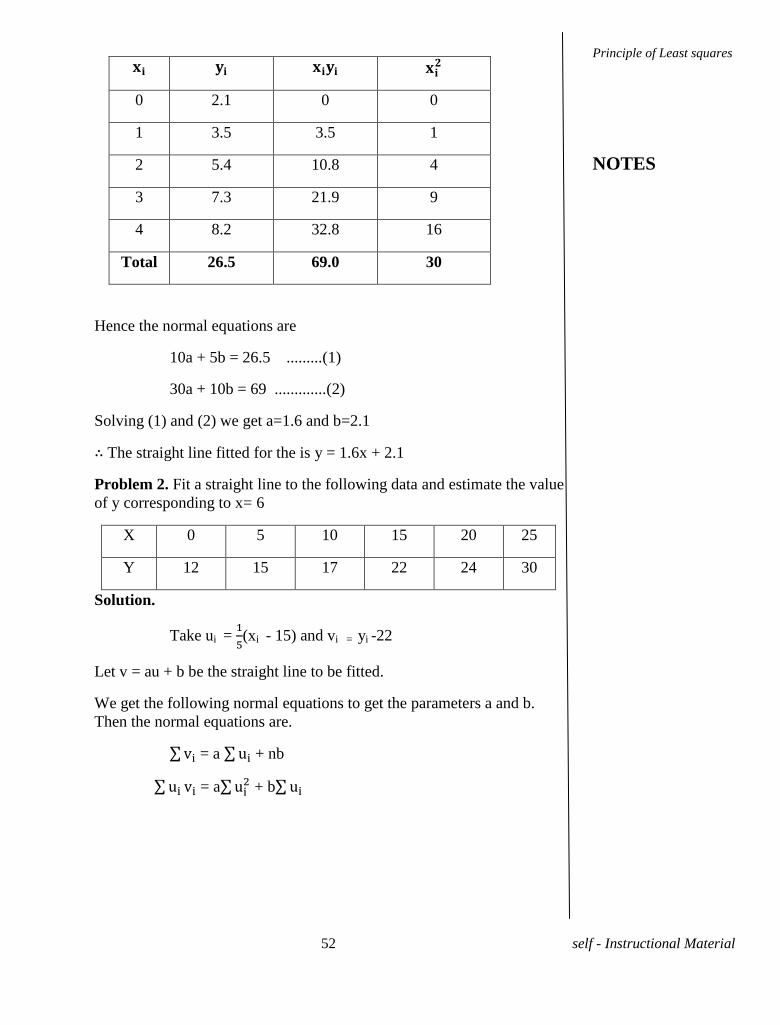
52 self - Instructional Material
0 2.1 0 0
1 3.5 3.5 1
2 5.4 10.8 4
3 7.3 21.9 9
4 8.2 32.8 16
Total 26.5 69.0 30
Hence the normal equations are
10a + 5b = 26.5 .........(1)
30a + 10b = 69 .............(2)
Solving (1) and (2) we get a=1.6 and b=2.1
∴ The straight line fitted for the is y = 1.6x + 2.1
Problem 2. Fit a straight line to the following data and estimate the value
of y corresponding to x= 6
X 0 5 10 15 20 25
Y 12 15 17 22 24 30
Solution.
Take ui =
(xi - 15) and vi = yi -22
Let v = au + b be the straight line to be fitted.
We get the following normal equations to get the parameters a and b.
Then the normal equations are.
= a + nb
= a + b
Principle of Least squares
NOTES
53 self - Instructional Material
xi yi ui vi ui vi
0 12 -3 -10 30 9
5 15 -2 -7 14 4
10 17 -1 -5 5 1
15 22 0 0 0 0
20 24 1 2 2 1
25 30 2 8 16 4
Total - -3 -12 67 19
∴ The normal equations are
-3a + 6b=-12 .........(1)
19a – 3b=67 ..........(2)
Solving for a and b we get a=3.49 and b = -0.26
∴ The straight line to be fitted becomes y – 22 =3.49
- 0.26
∴ 5y -110= 3.49x – 52.35 -1.30
∴5y= 3.49x + 56.35
∴y = .698x + 11.27
Now for x = 6 the estimated value of y is y=.698 6 +11.27 = 15.458
Problem 3. Fit a second degree parabola by taking xi as the
independent variable.
X 0 1 2 3 4
Y 1 5 10 22 38
Solution
Let the second parabola to be fitted to the data be y
Y = a +bx +c Then we have the normal equations to find a,b,c.
a + b
+c =
a + b
+c i =
Principle of Least squares
NOTES
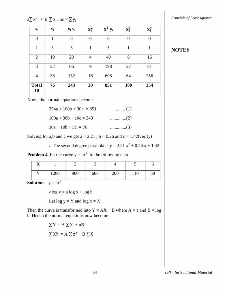
54 self - Instructional Material
a + i + nc =
xi yi xi yi
yi
0 1 0 0 0 0 0
1 5 5 1 5 1 1
2 10 20 4 40 8 16
3 22 66 9 198 27 81
4 38 152 16 608 64 256
Total
10
76 243 30 851 100 354
Now , the normal equations become
354a + 100b + 30c = 851 ............ (1)
100a + 30b + 10c = 243 ..............(2)
30a + 10b + 5c = 76 ..............(3)
Solving for a,b and c we get a = 2.21 ; b = 0.26 and c = 1.42(verify)
∴ The second degree parabola is y = 2.21 x2 + 0.26 x + 1.42
Problem 4. Fit the curve y = bxa to the following data.
X 1 2 3 4 5 6
Y 1200 900 600 200 110 50
Solution. y = bxa
∴log y = a log x + log b
Let log y = Y and log x = X
Then the curve is transformed into Y = AX + B where A = a and B = log
b. Hench the normal equations now become
= A + nB
= A + B
Principle of Least squares
NOTES
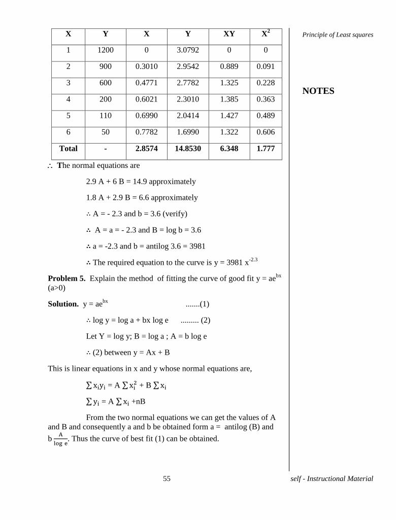
55 self - Instructional Material
X Y X Y XY X2
1 1200 0 3.0792 0 0
2 900 0.3010 2.9542 0.889 0.091
3 600 0.4771 2.7782 1.325 0.228
4 200 0.6021 2.3010 1.385 0.363
5 110 0.6990 2.0414 1.427 0.489
6 50 0.7782 1.6990 1.322 0.606
Total - 2.8574 14.8530 6.348 1.777
The normal equations are
2.9 A + 6 B = 14.9 approximately
1.8 A + 2.9 B = 6.6 approximately
∴ A = - 2.3 and b = 3.6 (verify)
∴ A = a = - 2.3 and B = log b = 3.6
∴ a = -2.3 and b = antilog 3.6 = 3981
∴ The required equation to the curve is y = 3981 x-2.3
Problem 5. Explain the method of fitting the curve of good fit y = aebx
(a>0)
Solution. y = aebx
.......(1)
∴ log y = log a + bx log e ......... (2)
Let Y = log y; B = log a ; A = b log e
∴ (2) between y = Ax + B
This is linear equations in x and y whose normal equations are,
= A + B
= A +nB
From the two normal equations we can get the values of A
and B and consequently a and b be obtained form a = antilog (B) and
b
. Thus the curve of best fit (1) can be obtained.
Principle of Least squares
NOTES
56 self - Instructional Material
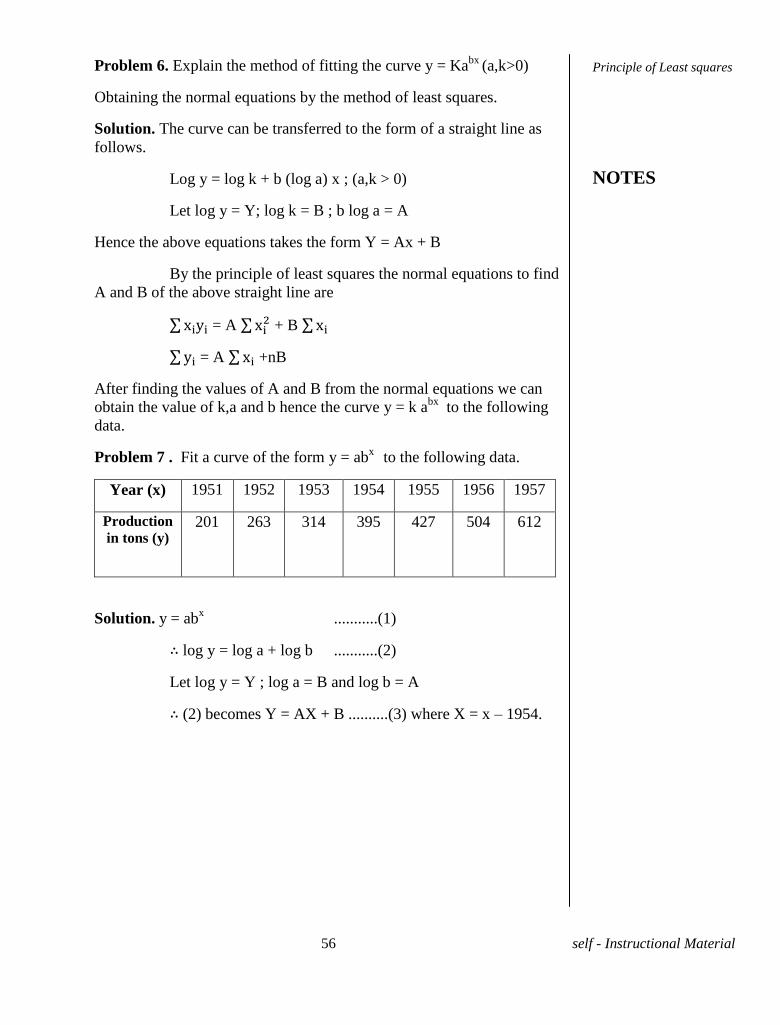
Problem 6. Explain the method of fitting the curve y = Kabx
(a,k>0)
Obtaining the normal equations by the method of least squares.
Solution. The curve can be transferred to the form of a straight line as
follows.
Log y = log k + b (log a) x ; (a,k > 0)
Let log y = Y; log k = B ; b log a = A
Hence the above equations takes the form Y = Ax + B
By the principle of least squares the normal equations to find
A and B of the above straight line are
= A + B
= A +nB
After finding the values of A and B from the normal equations we can
obtain the value of k,a and b hence the curve y = k abx
to the following
data.
Problem 7 . Fit a curve of the form y = abx
to the following data.
Year (x) 1951 1952 1953 1954 1955 1956 1957
Production
in tons (y) 201 263 314 395 427 504 612
Solution. y = abx
...........(1)
∴ log y = log a + log b ...........(2)
Let log y = Y ; log a = B and log b = A
∴ (2) becomes Y = AX + B ..........(3) where X = x – 1954.
Principle of Least squares
NOTES
57 self - Instructional Material
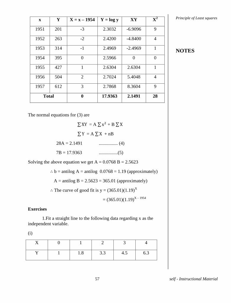
x Y X = x – 1954 Y = log y XY X2
1951 201 -3 2.3032 -6.9096 9
1952 263 -2 2.4200 -4.8400 4
1953 314 -1 2.4969 -2.4969 1
1954 395 0 2.5966 0 0
1955 427 1 2.6304 2.6304 1
1956 504 2 2.7024 5.4048 4
1957 612 3 2.7868 8.3604 9
Total 0 17.9363 2.1491 28
The normal equations for (3) are
= A + B
= A + nB
28A = 2.1491 ................ (4)
7B = 17.9363 ................(5)
Solving the above equation we get A = 0.0768 B = 2.5623
∴ b = antilog A = antilog 0.0768 = 1.19 (approximately)
A = antilog B = 2.5623 = 365.01 (approximately)
∴ The curve of good fit is y = (365.01)(1.19)X
= (365.01)(1.19)
X – 1954
Exercises
1.Fit a straight line to the following data regarding x as the
independent variable.
(i)
X 0 1 2 3 4
Y 1 1.8 3.3 4.5 6.3
Principle of Least squares
NOTES
58 self - Instructional Material
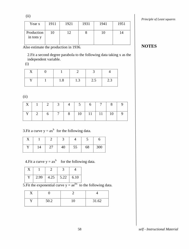
(ii)
Year x 1911 1921 1931 1941 1951
Production
in tons y
10 12 8 10 14
Also estimate the production in 1936.
2.Fit a second degree parabola to the following data taking x as the
independent variable.
(i)
X 0 1 2 3 4
Y 1 1.8 1.3 2.5 2.3
(ii)
X 1 2 3 4 5 6 7 8 9
Y 2 6 7 8 10 11 11 10 9
3.Fit a curve y = axb
for the following data.
4.Fit a curve y = axb
for the following data.
X 1 2 3 4
Y 2.99 4.25 5.22 6.10
5.Fit the exponential curve y = aebx
to the following data.
X 0 2 4
Y 50.2 10 31.62
X 1 2 3 4 5 6
Y 14 27 40 55 68 300
Principle of Least squares
NOTES
59 self - Instructional Material
UNIT-VII CORRELATION
7.1 INTRODUCTION
In statistical we have studied the methods of classifying
and analysing data relative to single variable. However data presenting
two sets of related observations may arise in many fields of activities
giving n pairs of corresponding observations ( i=1,2,..., n
For example, (i) of a colletion of students. (ii) may represent price of a commodity and
the corresponding demand. Such a data ( i=1,2,..., n is called a
bivariate data.
7.2 CORRELATION
Definition. Consider a set if bivariate data ( i=1,2,..., n. If there is
a change in one variable corresponding to change in the other variable
we say that the variables are correlated.
If the two variables deviate in the same direction the
correlation is said to be direct or positive. If they always deviate in the
opposite direction the correlation is said to be inverse or negative. If the
change in one variable corresponds to a proportional change in the other
variable then the correlation is said to be Perfect.
Height and weight of a batch of students; Income and
expenditure of a family are examples of variables with positive
correlation.
Price and demand; volume and pressure of a perfect
gas which obeys the law =k where k is a constant, are examples of
variables with negative correlation.
Definition. Karl Pereson's coefficient or correlation between the
variables x and y is defined by
where are the
arithmetic means and the standard deviations of the variables x
and y respectively.
Definition. The Covariance between x and y is defined by
cov(x,y)=
Hence
Correlation
NOTES
60 self - Instructional Material
Example. The heights and weights of five students are given below.
Height in c.m.
x
160 161 162 163 164
Weight in kgs.
y
50 53 54 56 57
Hence and (verify)
Now
= 17
=
=
9
Theorem 7.1.
Proof.
.....................(1)
Now, =
= +
=
=
=
....................(2)
Also,
=
=
=
=
Correlation
NOTES
61 self - Instructional Material
=
..............(3)
Similarly, =
................(4)
Substituting (2),(3) and (4) in (1) we get the required result.
The calculation of frequently be simplified by making
use of the following theorem.
Theorem 7.2 The correlation coefficient is independent of the change of
origin and scale.
Proof. Let
and
where h, k > 0.
and
Hence and
- ) and
Also and
=
=
Hence
Theorem 7.3 -1 ≤ ≤ 1
Proof.
=
Let and
=
By Schwartz inequality we have
Correlation
NOTES
62 self - Instructional Material
Hence
-1 ≤ ≤ 1
Note1. If = 1 the correlation is perfect and positive
Note 2. If = -1 the correlation is perfect and negative
Note 3. If = 0 the variables are uncorrelated.
Note 4. If the variables x and y are uncorrelated then Cov(x,y)= 0.
The following theorem gives another formula for
interms and
.
Theorem 7.4
Proof.
=
=
=
=
Solved Problems.
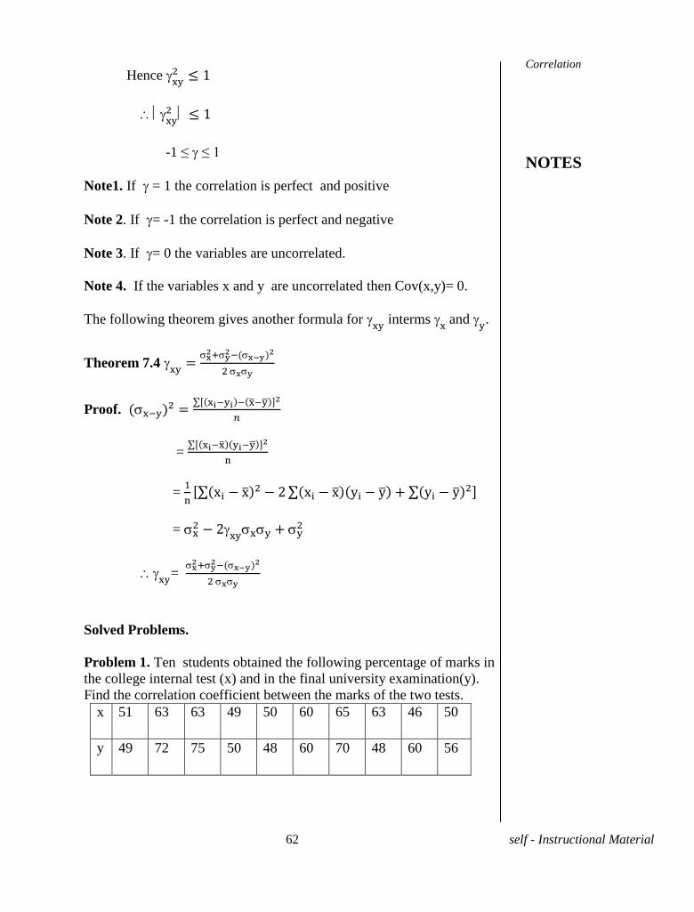
Problem 1. Ten students obtained the following percentage of marks in
the college internal test (x) and in the final university examination(y).
Find the correlation coefficient between the marks of the two tests.
x 51 63 63 49 50 60 65 63 46 50
y 49 72 75 50 48 60 70 48 60 56
Correlation
NOTES
63 self - Instructional Material
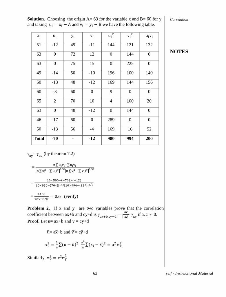
Solution. Choosing the origin A= 63 for the variable x and B= 60 for y
and taking and we have the following table.
51 -12 49 -11 144 121 132
63 0 72 12 0 144 0
63 0 75 15 0 225 0
49 -14 50 -10 196 100 140
50 -13 48 -12 169 144 156
60 -3 60 0 9 0 0
65 2 70 10 4 100 20
63 0 48 -12 0 144 0
46 -17 60 0 289 0 0
50 -13 56 -4 169 16 52
Total -70 - -12 980 994 200
=
(by theorem 7.2)
=
=
=
(verify)
Problem 2. If x and y are two variables prove that the correlation
coefficient between ax+b and cy+d is
Proof. Let u= ax+b and v = cy+d
= a +b and = c +d
=
Similarly,
Correlation
NOTES
64 self - Instructional Material
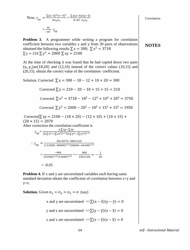
Now,
=
=
Problem 3. A programmer while writing a program for correlation
coefficient between two variables x and y from 30 pairs of observations
obtained the following results
At the time of checking it was found that he had copied down two pairs
( and (12,10) instead of the correct values (10,15) and
(20,15). obtain the correct value of the correlation coefficient.
Solution. Corrected
Corrected
Corrected
Corrected 9
Corrected After correction the correlation coefficient is
=
=
=
= -0.05
Problem 4. If x and y are uncorrelated variables each having same
standard deviation obtain the coefficient of correlation between x+y and
y+z.
Solution. Given (say)
x and y are uncorrelated =>
y and z are uncorrelated =>
z and x are uncorrelated =>
Correlation
NOTES
65 self - Instructional Material
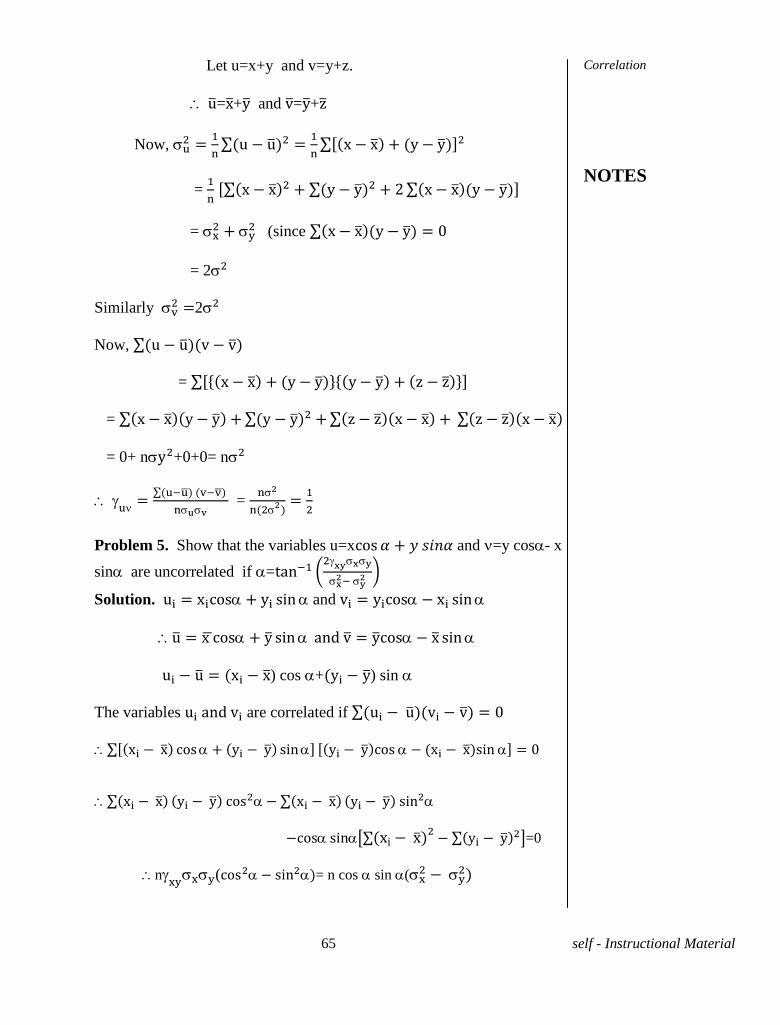
Let u=x+y and v=y+z.
= + and = +
Now,
=
=
(since
= 2
Similarly 2
Now,
=
=
= 0+ n +0+0= n
=
Problem 5. Show that the variables u=x and =y cos- x
sin are uncorrelated if =
Solution. and
) cos + ) sin
The variables are correlated if
=0
n ( = n cos sin (
Correlation
NOTES
66 self - Instructional Material
tan 2=
=
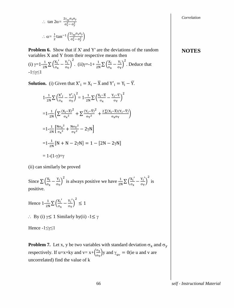
Problem 6. Show that if X' and Y' are the deviations of the random
variables X and Y from their respective means then
(i) =1-
. (ii) =-1+
. Deduce that
-1≤ ≤1
Solution. (i) Given that and
1-
= 1-
=1-
=1-
=1-
= 1-(1- )=
(ii) can similarly be proved
Since
is always positive we have
is
positive.
Hence 1-
By (i) Similarly by(ii) -1
Hence -1≤ ≤1
Problem 7. Let x, y be two variables with standard deviation
respectively. If u=x+ky and v= x+
y and
(ie u and v are
uncorrelated) find the value of k
Correlation
NOTES
67 self - Instructional Material
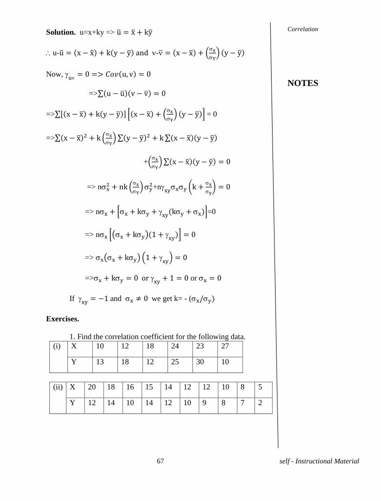
Solution. u=x+ky =>
u- -
Now,
=>
=>
= 0
=>
+
=> n
+n
=> n =0
=> n
=>
=> or
If and we get k= - (
Exercises.
1. Find the correlation coefficient for the following data.
(i) X 10 12 18 24 23 27
Y 13 18 12 25 30 10
(ii) X 20 18 16 15 14 12 12 10 8 5
Y 12 14 10 14 12 10 9 8 7 2
Correlation
NOTES
68 self - Instructional Material
(iii) Age of
husband
23 27 28 29 30 31 33 35 36 39
Age of
wife
18 22 23 24 25 26 28 29 30 32
7.3 RANK CORRELATION
Suppose that a group of n individuals are arranged in the order of
merit or efficiency with respect to some characteristics. Then the rank is
a variable which takes only the values1, 2, 3,....., n assuming that there is
no tie. Hence
and the variance is given by
Now suppose that the same individuals are ranked in two ways on
the basis of different characteristics or by two different persons for a
single characteristics . Let be the ranks of the individual in
the first and second ranking respectively. The coefficient of correlation
between the ranks is called the rank correlation coefficient and
is denoted by
Theorem 7.5. Rank correlation is given by =1-
Proof. Consider a collection of n individuals. Let be the ranks
of individual
in the two different rankings.
and
Now, (sice )
=
= n
-2n
= 2n (since
)
=
=1-
Correlation
NOTES
69 self - Instructional Material
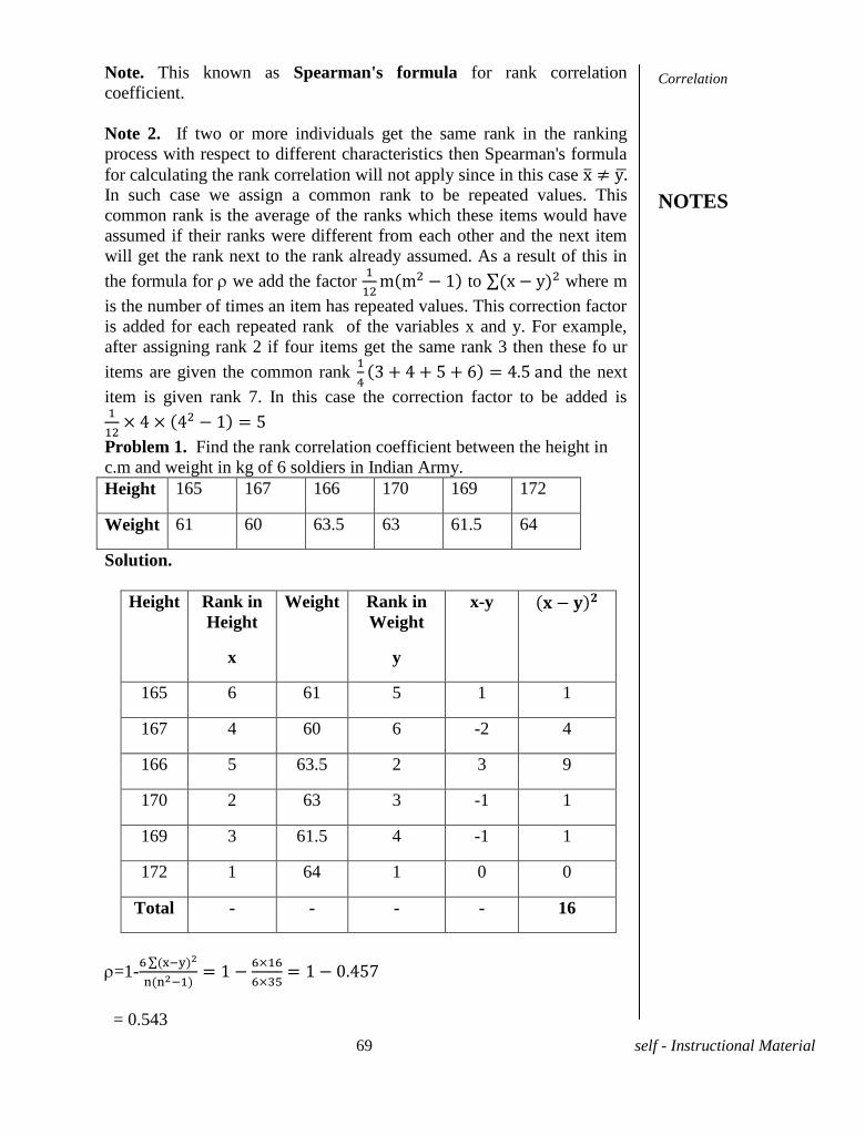
Note. This known as Spearman's formula for rank correlation
coefficient.
Note 2. If two or more individuals get the same rank in the ranking
process with respect to different characteristics then Spearman's formula
for calculating the rank correlation will not apply since in this case
In such case we assign a common rank to be repeated values. This
common rank is the average of the ranks which these items would have
assumed if their ranks were different from each other and the next item
will get the rank next to the rank already assumed. As a result of this in
the formula for we add the factor
to where m
is the number of times an item has repeated values. This correction factor
is added for each repeated rank of the variables x and y. For example,
after assigning rank 2 if four items get the same rank 3 then these fo ur
items are given the common rank
the next
item is given rank 7. In this case the correction factor to be added is
Problem 1. Find the rank correlation coefficient between the height in
c.m and weight in kg of 6 soldiers in Indian Army.
Height 165 167 166 170 169 172
Weight 61 60 63.5 63 61.5 64
Solution.
Height Rank in
Height
x
Weight Rank in
Weight
y
x-y
165 6 61 5 1 1
167 4 60 6 -2 4
166 5 63.5 2 3 9
170 2 63 3 -1 1
169 3 61.5 4 -1 1
172 1 64 1 0 0
Total - - - - 16
=1-
= 0.543
Correlation
NOTES
70 self - Instructional Material
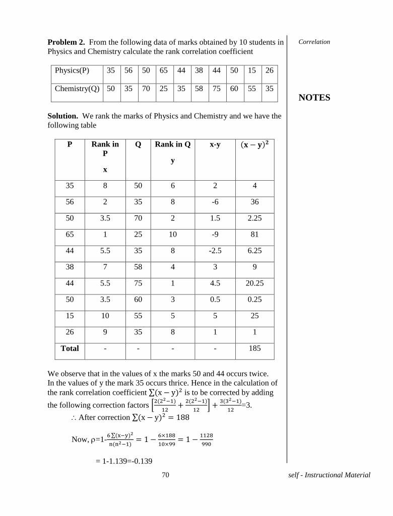
Problem 2. From the following data of marks obtained by 10 students in
Physics and Chemistry calculate the rank correlation coefficient
Physics(P) 35 56 50 65 44 38 44 50 15 26
Chemistry(Q) 50 35 70 25 35 58 75 60 55 35
Solution. We rank the marks of Physics and Chemistry and we have the
following table
P Rank in
P
x
Q Rank in Q
y
x-y
35 8 50 6 2 4
56 2 35 8 -6 36
50 3.5 70 2 1.5 2.25
65 1 25 10 -9 81
44 5.5 35 8 -2.5 6.25
38 7 58 4 3 9
44 5.5 75 1 4.5 20.25
50 3.5 60 3 0.5 0.25
15 10 55 5 5 25
26 9 35 8 1 1
Total - - - - 185
We observe that in the values of x the marks 50 and 44 occurs twice.
In the values of y the mark 35 occurs thrice. Hence in the calculation of
the rank correlation coefficient is to be corrected by adding
the following correction factors
=3.
After correction
Now, =1-
= 1-1.139=-0.139
Correlation
NOTES
71 self - Instructional Material
Problem 3. Three judges assign the ranks to 8 entries in a beauty contest.
Judge
in X
1 2 4 3 7 6 5 8
Judge
in Y
3 2 1 5 4 7 6 8
Judge
in Z
1 2 3 4 5 7 8 6
which pair of judges has the nearest approach to common taste in beauty?
Solution.
x Y z x-y y-z z-x
1 3 1 -2 4 2 4 0 0
2 2 2 0 0 0 0 0 0
4 1 3 3 9 -2 4 -1 1
3 5 4 -2 4 1 1 1 1
7 4 5 3 9 -1 1 -2 4
6 7 7 -1 1 0 0 1 1
5 6 8 -1 1 -2 4 3 9
8 8 6 0 0 2 4 -2 4
Total - 28 - 18 - 20
= 1-
=1-
=1-
1-0.333=0.667
=1-
= 0.762
Since
is greater than
and
the judges Mr.Y and Mr.Z have
nearest approach to common taste in beauty.
Correlation
NOTES
72 self - Instructional Material
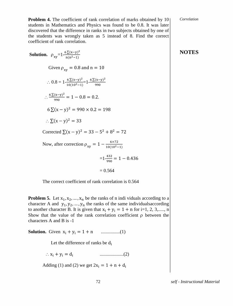
Problem 4. The coefficient of rank correlation of marks obtained by 10
students in Mathematics and Physics was found to be 0.8. It was later
discovered that the difference in ranks in two subjects obtained by one of
the students was wrongly taken as 5 instead of 8. Find the correct
coefficient of rank correlation.
Solution.
=1-
Given
0.8 = 1-
=1-
99 9
Corrected
Now, after correction
=1-
= 0.564
The correct coefficient of rank correlation is 0.564
Problem 5. Let be the ranks of n indi viduals according to a
character A and the ranks of the same individualsaccording
to another character B. It is given that for i=1, 2, 3,....., n
Show that the value of the rank correlation coefficient between the
characters A and B is -1
Solution. Given ................(1)
Let the difference of ranks be
....................(2)
Adding (1) and (2) we get 2
Correlation
NOTES
73 self - Instructional Material
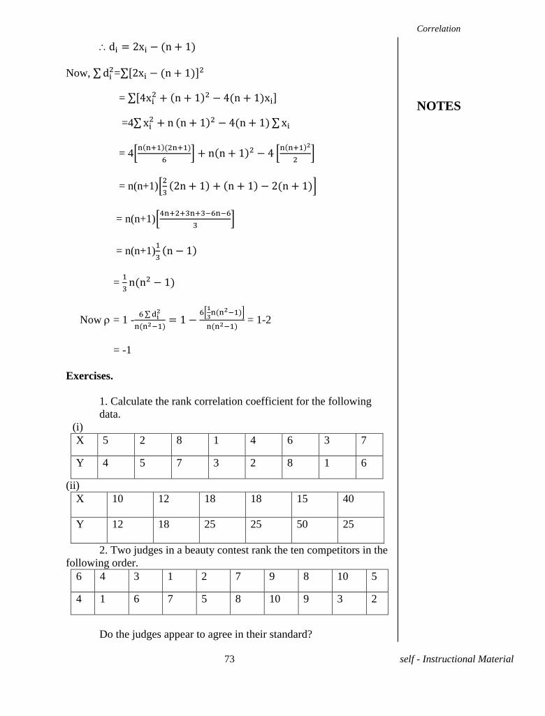
Now, =
=
=4
= 4
= n(n+1)
= n(n+1)
= n(n+1)
=
Now = 1 -
= 1-2
= -1
Exercises.
1. Calculate the rank correlation coefficient for the following
data.
(i)
X 5 2 8 1 4 6 3 7
Y 4 5 7 3 2 8 1 6
(ii)
X 10 12 18 18 15 40
Y 12 18 25 25 50 25
2. Two judges in a beauty contest rank the ten competitors in the
following order.
6 4 3 1 2 7 9 8 10 5
4 1 6 7 5 8 10 9 3 2
Do the judges appear to agree in their standard?
Correlation
NOTES
74 self - Instructional Material
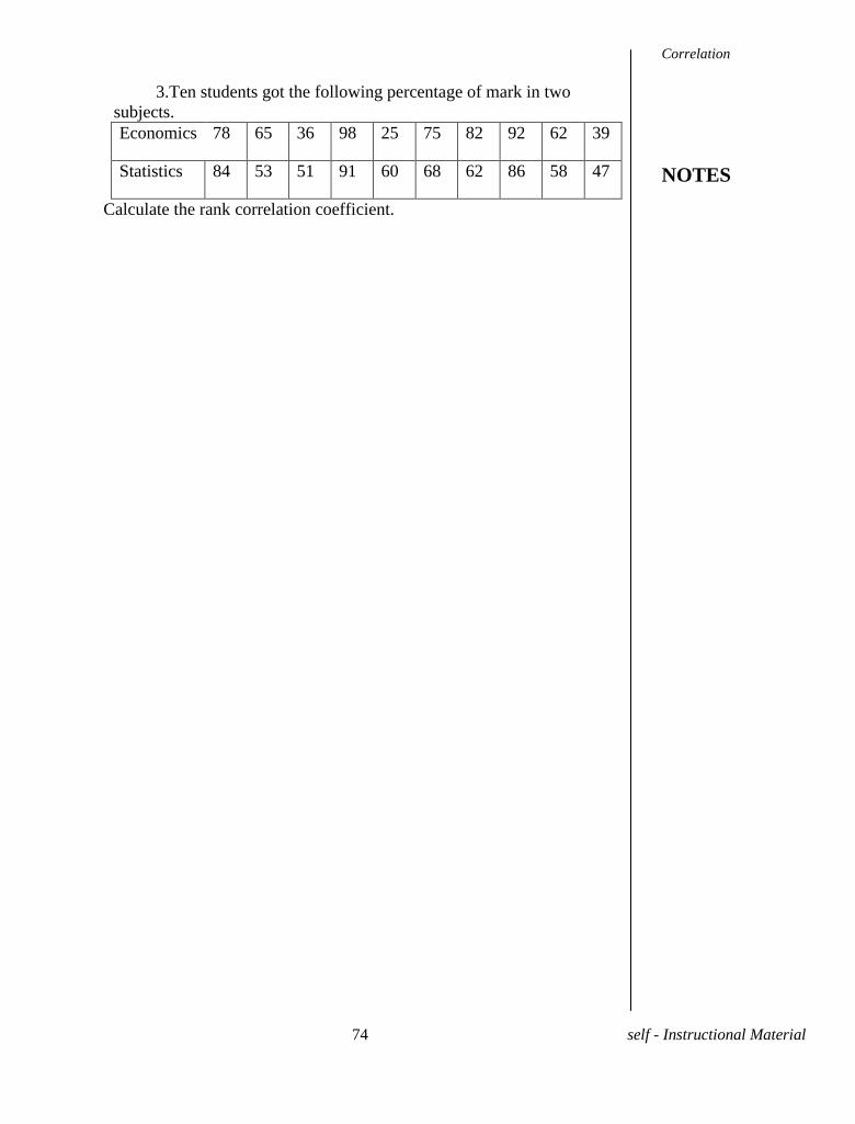
3.Ten students got the following percentage of mark in two
subjects.
Economics 78 65 36 98 25 75 82 92 62 39
Statistics 84 53 51 91 60 68 62 86 58 47
Calculate the rank correlation coefficient.
Correlation
NOTES
75 self - Instructional Material
UNIT-VIII REGRESSION
8.1 INTRODUCTION
There are two main problems involved in the relationship
between x and y. The first is to find a measure of the degree of
association or correlation between the values of x and those of y. The
second problem is to find the most suitable form of equation for
determining the probable value of one variable corresponding to a given
value of the order. This is the problem of regression.
If there is a functional relationship between the two variables
the points in the scatter diagram will cluster around some curve
called the curve of regression. If the curve is straight line it is called a
line of regression between the two variables.
8.2 Definition. It we fit a straight line by the principle of least square to
the points of the scatter diagram in such a way that the sum of the squares
of the distance parallel to the y-axis from the points to the line is
minimized we obtain a line of best fit for the data and it is called the
regression line of y on x.
Similarly we can define the regression line of x on y.
Theorem 8.1 The equation of the regression line of y on x is given by
y-
Proof. Let y=ax+b be the line of regression of y on x.
According to the principle of least squares constants a and b are
to be determined in such a way that S= is minimum.
=a +b .................(1)
> a +nb ...............(2)
Equations (1) and (2) are called normal equations.
From (2) we obtain ...............(3)
Regression
NOTES
76 self - Instructional Material
The line of regression passes through the point ( Now Shifting the origin to this point ( by means of the
transformation and we obtain And the equation of the line of regression becomes Y=aX ...........(4)
Corresponding to this line Y=aX, the constant a can be
determined from the normal equation. a
a=
The required regression line (4) becomes Y=
Theorem 8.2 The equation of regression line of x on y is given by
Proof. Proof is similar to that of theorem 8.1
Note. ( is the point of intersection of the two regression lines.
Definition. The slope of the regression line of y on x is called the
regression coefficient of y on x and it is denoted by Hence
The regression coefficient of x on y is given by
We now give some properties of the regression coefficients.
Theorem 8.3. Correlation coefficient is the geometric mean between
the regression coefficients. (i.e) =±
Proof. We have
=±
Note. The sign of the correlation coefficient is the same as that of
regression coefficients.
Regression
NOTES
77 self - Instructional Material
Theorem 8.4. If one of the regression coefficient is greater than unity
the other is less than unity.
Proof. We have so that
Hence
Hence the theorem.
Theorem 8.5. Arithmetic mean of the regression coefficients is greater
than or equal to the correlation coefficient.
Proof. Let and be the regression coefficients.
We have to prove that
Now ,
-2
(
This is always true. Hence the theorem.
Theorem 8.6 Regression coefficients are independent of the change of
origin but dependent on change of scale.
Proof. Let
and
Let
We know that and
Now,
=
=
........... (1)
Similarly
.......................(2)
From (1) and (2) we observe that depend upon the scales h
and k but not on the origin A and B.
Hence the theorem.
Regression
NOTES
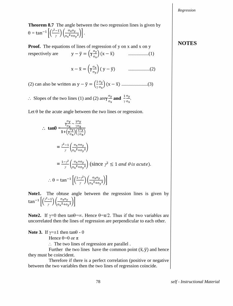
78 self - Instructional Material
Theorem 8.7 The angle between the two regression lines is given by
=
Proof. The equations of lines of regression of y on x and x on y
respectively are
.................(1)
..................(2)
(2) can also be written as
......................(3)
Slopes of the two lines (1) and (2) are
and
Let be the acute angle between the two lines or regression.
tan =
=
=
(since
=
Note1. The obtuse angle between the regression lines is given by
Note2. If =0 then tan=∞. Hence =π/2. Thus f he w v r b es re
uncorrelated then the lines of regression are perpendicular to each other.
Note 3. If =±1 then tan - 0
Hence =0 r π
The two lines of regression are parallel .
Further the two lines have the common point ( and hence
they must be coincident.
Therefore if there is a perfect correlation (positive or negative
between the two variables then the two lines of regression coincide.
Regression
NOTES
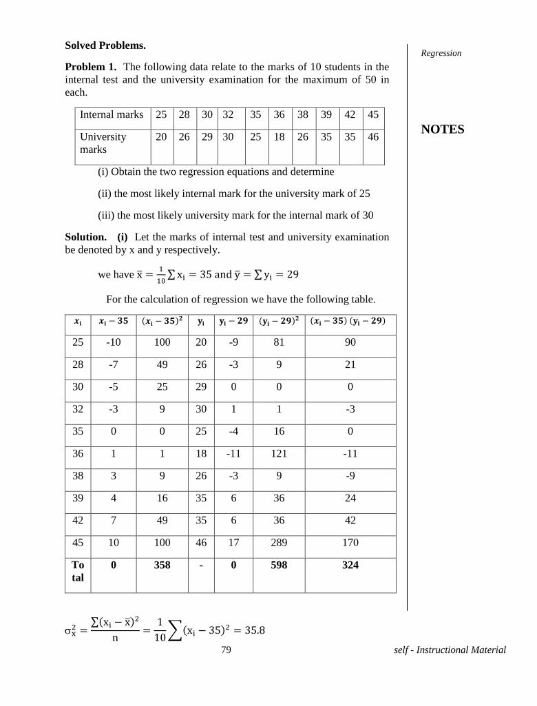
79 self - Instructional Material
Solved Problems.
Problem 1. The following data relate to the marks of 10 students in the
internal test and the university examination for the maximum of 50 in
each.
Internal marks 25 28 30 32 35 36 38 39 42 45
University
marks
20 26 29 30 25 18 26 35 35 46
(i) Obtain the two regression equations and determine
(ii) the most likely internal mark for the university mark of 25
(iii) the most likely university mark for the internal mark of 30
Solution. (i) Let the marks of internal test and university examination
be denoted by x and y respectively.
we have
9
For the calculation of regression we have the following table.
25 -10 100 20 -9 81 90
28 -7 49 26 -3 9 21
30 -5 25 29 0 0 0
32 -3 9 30 1 1 -3
35 0 0 25 -4 16 0
36 1 1 18 -11 121 -11
38 3 9 26 -3 9 -9
39 4 16 35 6 36 24
42 7 49 35 6 36 42
45 10 100 46 17 289 170
To
tal
0 358 - 0 598 324
Regression
NOTES
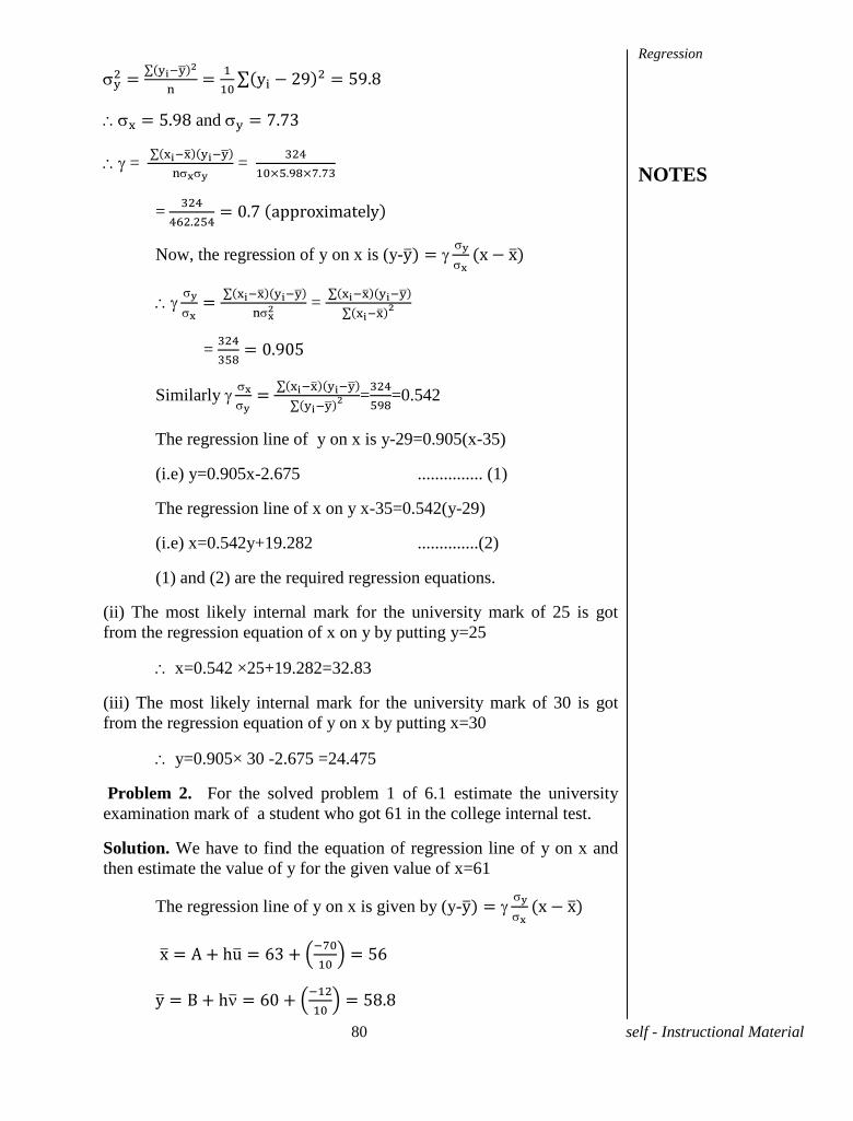
80 self - Instructional Material
9 9
9 and
=
=
=
Now, the regression of y on x is (y-
=
=
9
Similarly
=
=0.542
The regression line of y on x is y-29=0.905(x-35)
(i.e) y=0.905x-2.675 ............... (1)
The regression line of x on y x-35=0.542(y-29)
(i.e) x=0.542y+19.282 ..............(2)
(1) and (2) are the required regression equations.
(ii) The most likely internal mark for the university mark of 25 is got
from the regression equation of x on y by putting y=25
x=0.542 ×25+19.282=32.83
(iii) The most likely internal mark for the university mark of 30 is got
from the regression equation of y on x by putting x=30
y=0.905× 30 -2.675 =24.475
Problem 2. For the solved problem 1 of 6.1 estimate the university
examination mark of a student who got 61 in the college internal test.
Solution. We have to find the equation of regression line of y on x and
then estimate the value of y for the given value of x=61
The regression line of y on x is given by (y-
Regression
NOTES
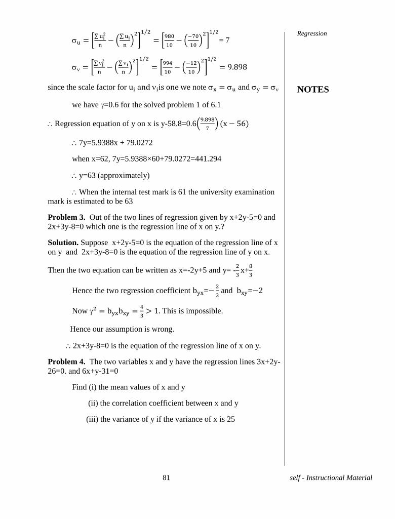
81 self - Instructional Material
= 7
9 9
since the scale factor for note and
we have =0.6 for the solved problem 1 of 6.1
Regression equation of y on x is y-58.8=0.6
7y=5.9388x + 79.0272
when x=62, 7y=5.9388×60+79.0272=441.294
y=63 (approximately)
When the internal test mark is 61 the university examination
mark is estimated to be 63
Problem 3. Out of the two lines of regression given by x+2y-5=0 and
2x+3y-8=0 which one is the regression line of x on y.?
Solution. Suppose x+2y-5=0 is the equation of the regression line of x
on y and 2x+3y-8=0 is the equation of the regression line of y on x.
Then the two equation can be written as x=-2y+5 and y= -
+
Hence the two regression coefficient =
and =
Now
This is impossible.
Hence our assumption is wrong.
2x+3y-8=0 is the equation of the regression line of x on y.
Problem 4. The two variables x and y have the regression lines 3x+2y-
26=0. and 6x+y-31=0
Find (i) the mean values of x and y
(ii) the correlation coefficient between x and y
(iii) the variance of y if the variance of x is 25
Regression
NOTES
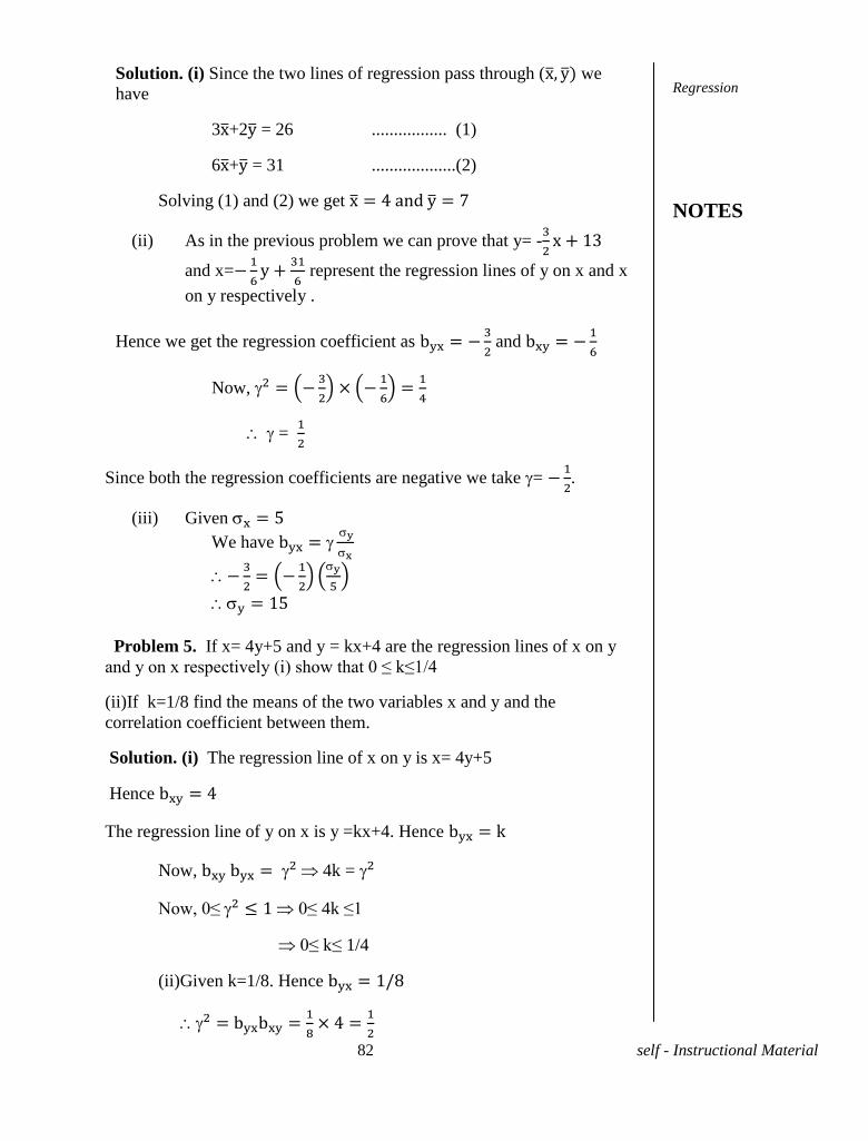
82 self - Instructional Material
Solution. (i) Since the two lines of regression pass through ( we
have
3 +2 = 26 ................. (1)
6 + = 31 ...................(2)
Solving (1) and (2) we get
(ii) As in the previous problem we can prove that y= -
and x=
represent the regression lines of y on x and x
on y respectively .
Hence we get the regression coefficient as
and
Now,
=
Since both the regression coefficients are negative we take =
.
(iii) Given
We have
Problem 5. If x= 4y+5 and y = kx+4 are the regression lines of x on y
d y x respec ve y ( ) sh w h 0 ≤ k≤1/4
(ii)If k=1/8 find the means of the two variables x and y and the
correlation coefficient between them.
Solution. (i) The regression line of x on y is x= 4y+5
Hence
The regression line of y on x is y =kx+4. Hence
Now, 4k =
N w, 0≤ 0≤ 4k ≤1
0≤ k≤ 1/4
(ii)Given k=1/8. Hence
Regression
NOTES
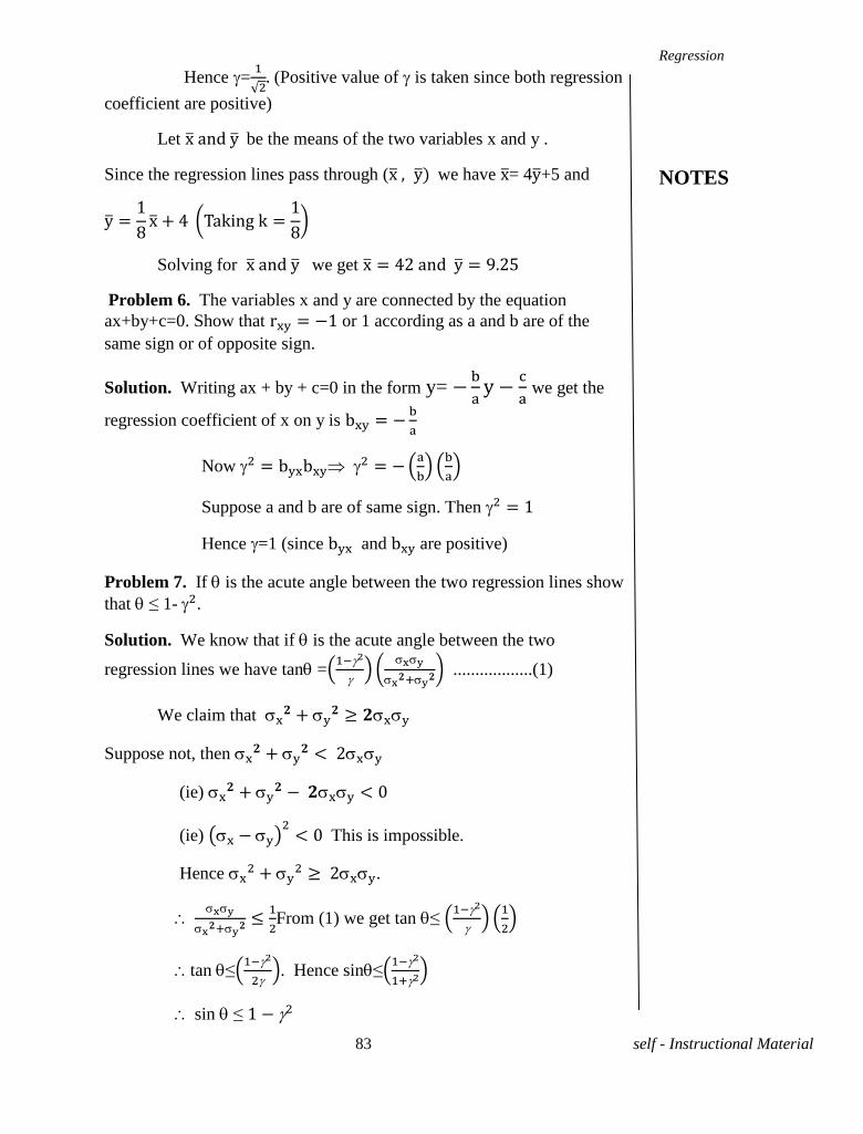
83 self - Instructional Material
Hence =
(Positive value of is taken since both regression
coefficient are positive)
Let be the means of the two variables x and y .
Since the regression lines pass through ( we have = 4 +5 and
Solving for we get 9
Problem 6. The variables x and y are connected by the equation
ax+by+c=0. Show that or 1 according as a and b are of the
same sign or of opposite sign.
Solution. Writing ax + by + c=0 in the form y=
we get the
regression coefficient of x on y is
Now
Suppose a and b are of same sign. Then
Hence =1 (since and are positive)
Problem 7. If is the acute angle between the two regression lines show
that ≤ 1- .
Solution. We know that if is the acute angle between the two
regression lines we have tan =
..................(1)
We claim that
Suppose not, then
(ie)
(ie) This is impossible.
Hence
.
From (1) we get tan ≤
tan ≤
. Hence sin≤
sin ≤
Regression
NOTES
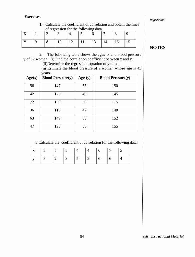
84 self - Instructional Material
Exercises.
1. Calculate the coefficient of correlation and obtain the lines
of regression for the following data.
X 1 2 3 4 5 6 7 8 9
Y 9 8 10 12 11 13 14 16 15
2. The following table shows the ages x and blood pressure
y of 12 women. (i) Find the correlation coefficient between x and y.
(ii)Determine the regression equation of y on x.
(iii)Estimate the blood pressure of a women whose age is 45
years.
Age(x) Blood Pressure(y) Age (y) Blood Pressure(y)
56 147 55 150
42 125 49 145
72 160 38 115
36 118 42 140
63 149 68 152
47 128 60 155
3.Calculate the coefficient of correlation for the following data.
x 3 6 5 4 4 6 7 5
y 3 2 3 5 3 6 6 4
Regression
NOTES
85 self - Instructional Material
UNIT-IX CORRELATION
COEFFICIENT FOR A BIVARIATE
FREQUENCY DISTRIBUTION
9.1 INTRODUTION :
As in the case of a single variable large collection of data
corresponding to two variables under consideration can also be
conveniently summarised in a 2-way frequency table (bivariate frequency
table)which is illustrated below.
If there are n classes for the first variable x and m classes for the
second variable y then there are mn cells in the 2 - way table. If xi and yi
denote the mid values of the ith
class for x and jth
class for y respectively
then the frequency fij corressponding to (xi yi) is entered in the (i,j)th
cell.
For i = 1,2,.....,n and j = 1,2,....,m we get all the mn cells, in the table.
From the bivariate frequency table we note the following :
(1) For any fixed i we have 1
m
ij
j
f
= gi = the sum of all the cell
frequencies of the ith column.
(2) For any fixed j we have 1
n
ij
i
f
= fj = the sum of the cell frequencies
of the jth row.
Correlation Coefficient for a
Bivariate frequency
Distribution
NOTES
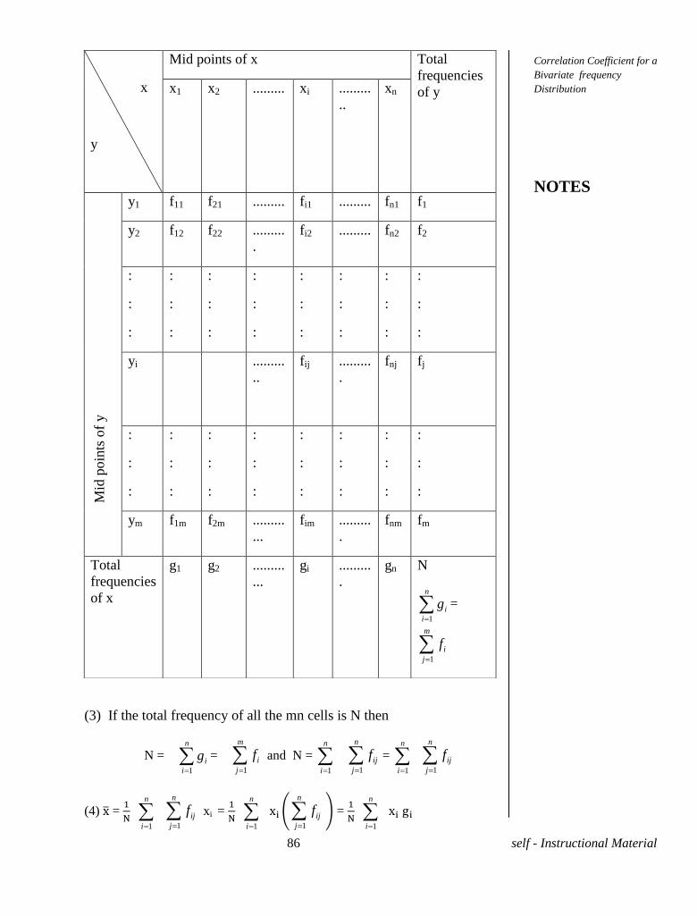
86 self - Instructional Material
(3) If the total frequency of all the mn cells is N then
N = 1
n
i
i
g
= 1
m
i
j
f
and N = 1
n
i
1
n
ij
j
f
= 1
n
i
1
n
ij
j
f
(4) =
1
n
i
1
n
ij
j
f
xi =
1
n
i
1
n
ij
j
f
=
1
n
i
x
y
Mid points of x Total
frequencies
of y x1 x2 ......... xi .........
..
xn M
id p
oin
ts o
f y
y1 f11 f21 ......... fi1 ......... fn1 f1
y2 f12 f22 .........
.
fi2 ......... fn2 f2
:
:
:
:
:
:
:
:
:
:
:
:
:
:
:
:
:
:
:
:
:
:
:
:
yi .........
..
fij .........
.
fnj fj
:
:
:
:
:
:
:
:
:
:
:
:
:
:
:
:
:
:
:
:
:
:
:
:
ym f1m f2m .........
...
fim .........
.
fnm fm
Total
frequencies
of x
g1 g2 .........
...
gi .........
.
gn N
1
n
i
i
g
=
1
m
i
j
f
Correlation Coefficient for a
Bivariate frequency
Distribution
NOTES
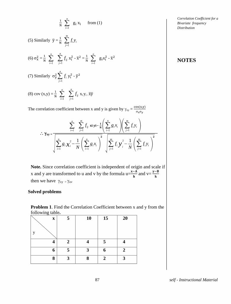
87 self - Instructional Material
1
n
i
from (1)
(5) Similarly =
1
m
i i
j
f y
(6) =
1
n
i
1
n
ij
j
f
- =
1
n
i
-
(7) Similarly
1
n
i
j
f
-
(8) cov (x,y) =
1
n
i
1
n
ij
j
f
xi yi -
The correlation coefficient between x and y is given by xy =
xy =
1
n
i
1
m
ij
j
f
1
n
i i
i
g x
1
m
i i
j
f y
2
1
1n
i ii
gN
x
1
n
i i
i
g x
2
1
1m
ii
j
fN
y
1
m
i i
j
f y
Note. Since correlation coefficient is independent of origin and scale if
x and y are transformed to u and v by the formula u=
and v=
then we have xy = uv
Solved problems
Problem 1. Find the Correlation Coefficient between x and y from the
following table.
x
y
5 10
15 20
4 2 4 5 4
6 5 3 6 2
8 3 8 2 3
Correlation Coefficient for a
Bivariate frequency
Distribution
NOTES
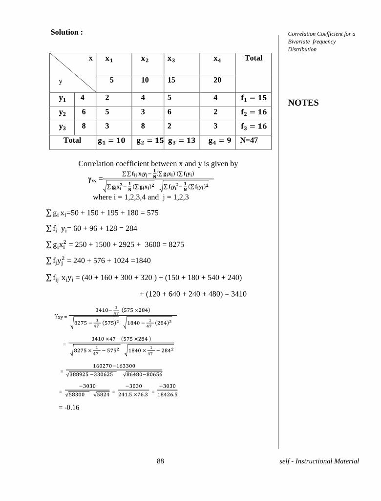
88 self - Instructional Material
Solution :
x
y
Total
5 10 15 20
4 2 4 5 4
6 5 3 6 2
8 3 8 2 3
Total N=47
Correlation coefficient between x and y is given by
xy =
where i = 1,2,3,4 and j = 1,2,3
=50 + 150 + 195 + 180 = 575
= 60 + 96 + 128 = 284
= 250 + 1500 + 2925 + 3600 = 8275
= 240 + 576 + 1024 =1840
= (40 + 160 + 300 + 320 ) + (150 + 180 + 540 + 240)
+ (120 + 640 + 240 + 480) = 3410
xy =
=
=
=
=
=
= -0.16
Correlation Coefficient for a
Bivariate frequency
Distribution
NOTES
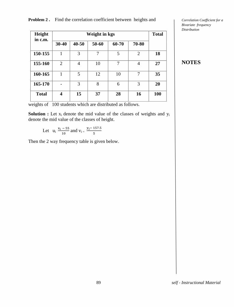
89 self - Instructional Material
Problem 2 . Find the correlation coefficient between heights and
weights of 100 students which are distributed as follows.
Solution : Let xi denote the mid value of the classes of weights and yi
denote the mid value of the classes of height.
Let ui
and vi =
Then the 2 way frequency table is given below.
Height
in c.m.
Weight in kgs Total
30-40 40-50 50-60 60-70 70-80
150-155 1 3 7 5 2 18
155-160 2 4 10 7 4 27
160-165 1 5 12 10 7 35
165-170 - 3 8 6 3 20
Total 4 15 37 28 16 100
Correlation Coefficient for a
Bivariate frequency
Distribution
NOTES
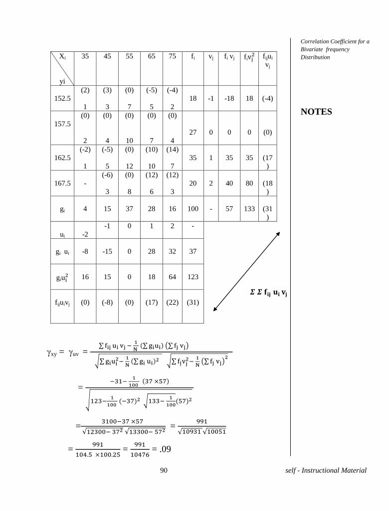
90 self - Instructional Material
xy = uv =
=
=
=
=
=
= .09
Xi
yi
35 45 55 65 75 fi vj fi vj fi fijui
vj
152.5
(2)
1
(3)
3
(0)
7
(-5)
5
(-4)
2
18
-1
-18
18
(-4)
157.5
(0)
2
(0)
4
(0)
10
(0)
7
(0)
4
27
0
0
0
(0)
162.5
(-2)
1
(-5)
5
(0)
12
(10)
10
(14)
7
35
1
35
35
(17
)
167.5
-
(-6)
3
(0)
8
(12)
6
(12)
3
20
2
40
80
(18
)
gi
4
15
37
28
16
100
-
57
133
(31
)
ui
-2
-1
0 1 2 -
gi ui
-8
-15
0
28
32
37
gi
16
15
0
18
64
123
fijuivj
(0)
(-8)
(0)
(17)
(22)
(31)
Correlation Coefficient for a
Bivariate frequency
Distribution
NOTES
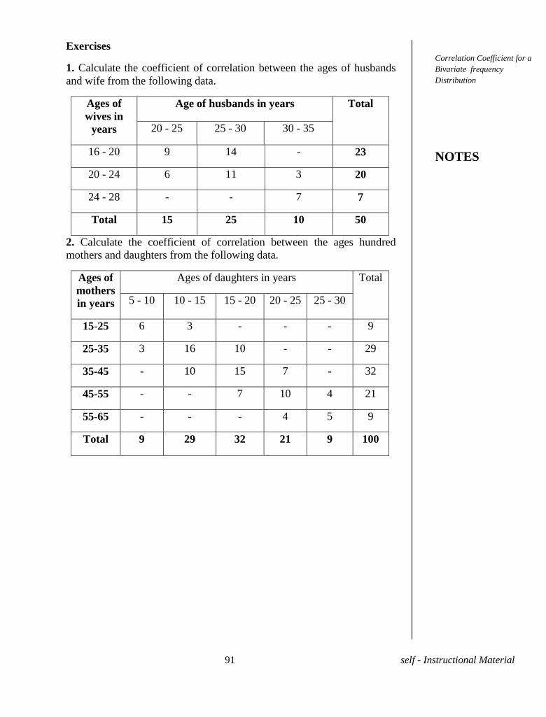
91 self - Instructional Material
Exercises
1. Calculate the coefficient of correlation between the ages of husbands
and wife from the following data.
Ages of
wives in
years
Age of husbands in years Total
20 - 25 25 - 30 30 - 35
16 - 20 9 14 - 23
20 - 24 6 11 3 20
24 - 28 - - 7 7
Total 15 25 10 50
2. Calculate the coefficient of correlation between the ages hundred
mothers and daughters from the following data.
Ages of
mothers
in years
Ages of daughters in years Total
5 - 10 10 - 15 15 - 20 20 - 25 25 - 30
15-25 6 3 - - - 9
25-35 3 16 10 - - 29
35-45 - 10 15 7 - 32
45-55 - - 7 10 4 21
55-65 - - - 4 5 9
Total 9 29 32 21 9 100
Correlation Coefficient for a
Bivariate frequency
Distribution
NOTES
92 self - Instructional Material
UNIT-X INTERPOLATION
10.1 INTRODUCTION
Definition. Interpolation is the process of finding the most appropriate
es m e f r m ss d . I s he “ r f re d be wee he es f
b e”. F r m k he m s pr b b e es m e requ res he f w
assumptions.
(i)The frequency distribution is normal and not marked by sudden ups
and downs.
(ii) The changes in the series are uniform within a period.
Interpolation technique is used in various disciplines like
economics, business, population studies, price determination etc, . It is
used to fill in the gaps in the statistical data for the sake of continuity of
information. For example, If we know the records for the past five years
except the third year which is not available due to unforeseen conditions
the interpolation technique helps to estimate the record for that year too
under the assumption that the changes in the records over these five years
have been uniform.
It is also possible that we may require information for future
inwhich case the process of estimating the most appropriate value is
known as extrapolation. There are two methods in interpolation.
(i) Graphic method
(ii) Algebraic method
(i)Graphic method is a simple method in which we just plot the
available data on a graph sheet and read off the value for the missing
period from the graph itself.
(ii) Algebraic method. There are several methods used for interpolation
of which we deal with the following: (i) Finite differences.
(ii) Gregory – New ’s f rmu
( )L r e’s f rmu
10.2 FINITE DIFFERENCES.
The operator ∆. is a function of the independent variable x and if a,
a+h, a+2h,........ are a finite set of equidistant values then
are the corresponding values for . The values of
the independent variable x are called arguments, the corresponding
values of are called entries and his known as the interval of
differencing. Hence is the entry for the argument a+h.
Interpolation
NOTES
93 self - Instructional Material
Definition. We def e per r ∆ wh ch s k w s he f rs rder
difference on s ∆ where x= a, a+h, a+2h,........ In
p r cu r ( ) ∆ ( ) ∆ If is constant .
Higher order differences can similarly be defined.
Example.
= ( ......................(1)
= +
Also from (1)
Note1. Unless otherwise stated interval of differencing is taken as 1.
Note 2. It is very easy to verify that the operator satisfies the basic
laws of algebra.
(i) is linear (ie) (a +b
(ii) satisfies the law of indices for multiplication.
(ie)
We can construct the difference table for any number arguments
and a sample difference table is exhibited below for five consecutive
arguments.
Interpolation
NOTES
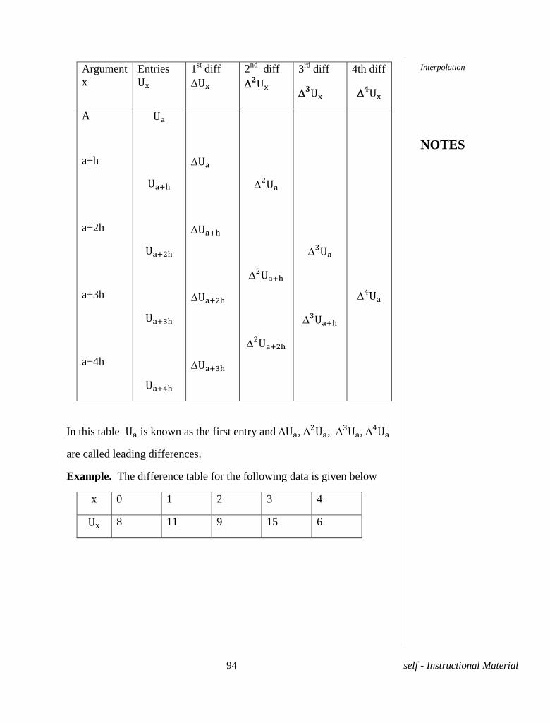
94 self - Instructional Material
Argument
x
Entries
1st diff
2nd
diff
3rd
diff
4th diff
A
a+h
a+2h
a+3h
a+4h
In this table is known as the first entry and , , ,
are called leading differences.
Example. The difference table for the following data is given below
x 0 1 2 3 4
8 11 9 15 6
Interpolation
NOTES
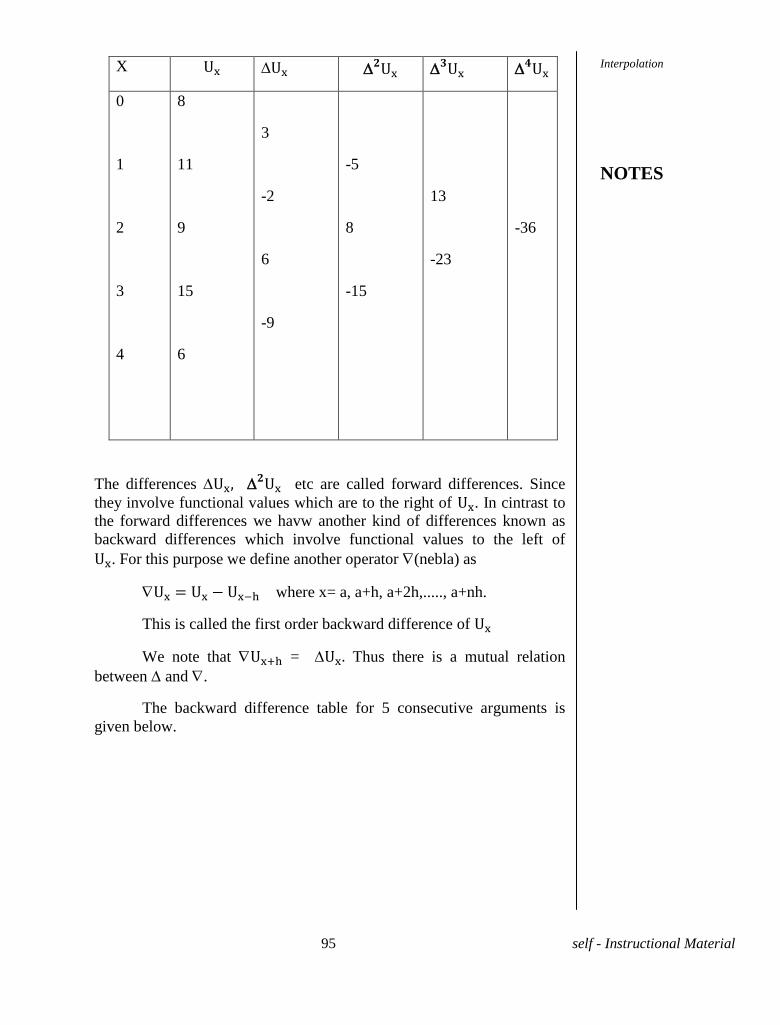
95 self - Instructional Material
X
0
1
2
3
4
8
11
9
15
6
3
-2
6
-9
-5
8
-15
13
-23
-36
The differences etc are called forward differences. Since
they involve functional values which are to the right of . In cintrast to
the forward differences we havw another kind of differences known as
backward differences which involve functional values to the left of . For this purpose we define another operator (nebla) as
where x= a, a+h, a+2h,....., a+nh.
This is called the first order backward difference of
We note that = Thus there is a mutual relation
between and .
The backward difference table for 5 consecutive arguments is
given below.
Interpolation
NOTES
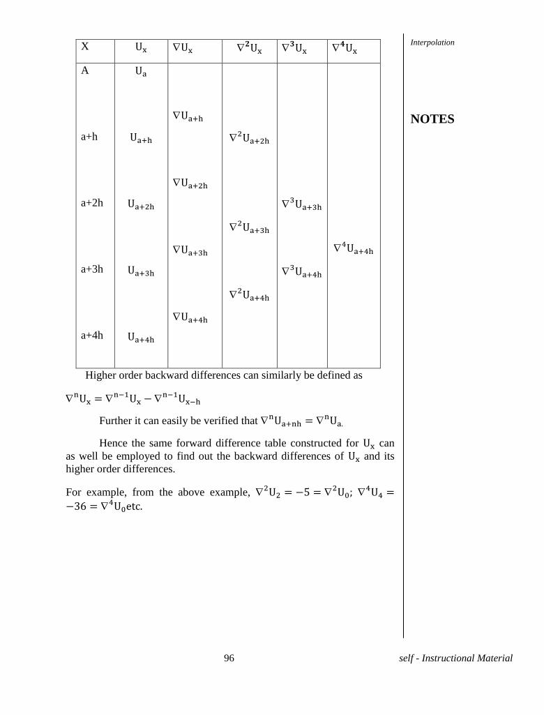
96 self - Instructional Material
X
A
a+h
a+2h
a+3h
a+4h
Higher order backward differences can similarly be defined as
Further it can easily be verified that
Hence the same forward difference table constructed for can
as well be employed to find out the backward differences of and its
higher order differences.
For example, from the above example,
Interpolation
NOTES
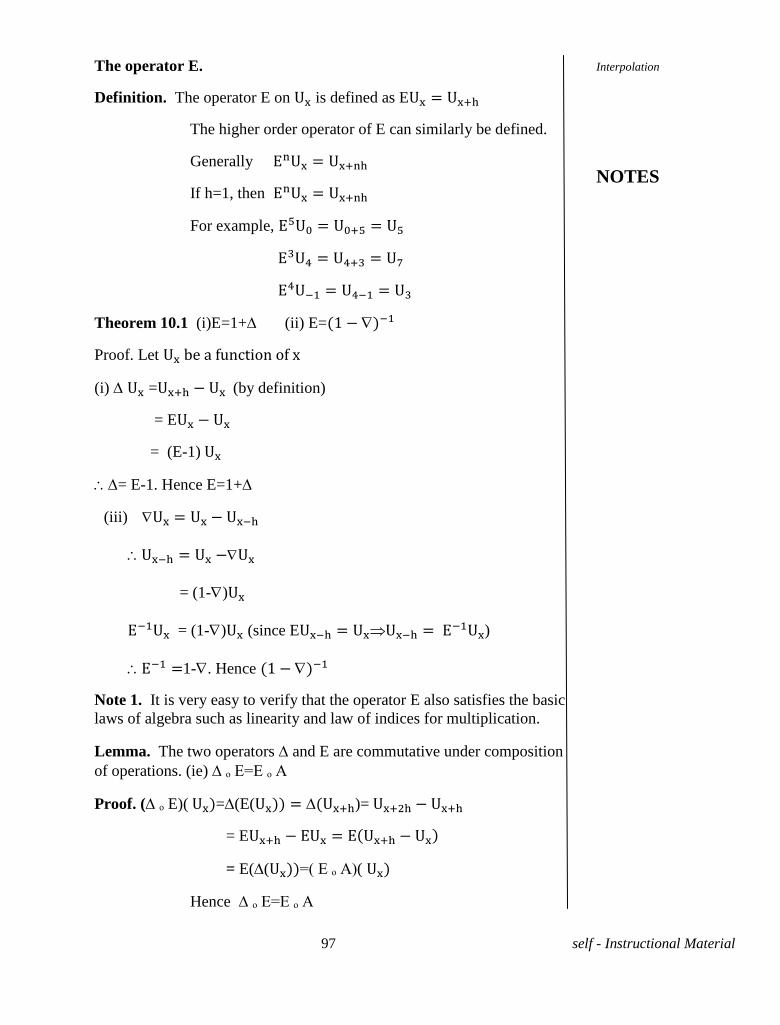
97 self - Instructional Material
The operator E.
Definition. The operator E on is defined as E
The higher order operator of E can similarly be defined.
Generally
If h=1, then
For example,
Theorem 10.1 (i)E=1+ (ii) E=
Proof. Let
(i) = (by definition)
= E
= (E-1)
= E-1. Hence E=1+
(iii)
= (1-)
= (1-) (since E )
1-. Hence
Note 1. It is very easy to verify that the operator E also satisfies the basic
laws of algebra such as linearity and law of indices for multiplication.
Lemma. The two operators and E are commutative under composition
of operations. (ie) ₒ E=E ₒ A
Proof. ( ₒ E)( = (E( )=
= E
= E( ( =( E ₒ A)(
Hence ₒ E=E ₒ A
Interpolation
NOTES
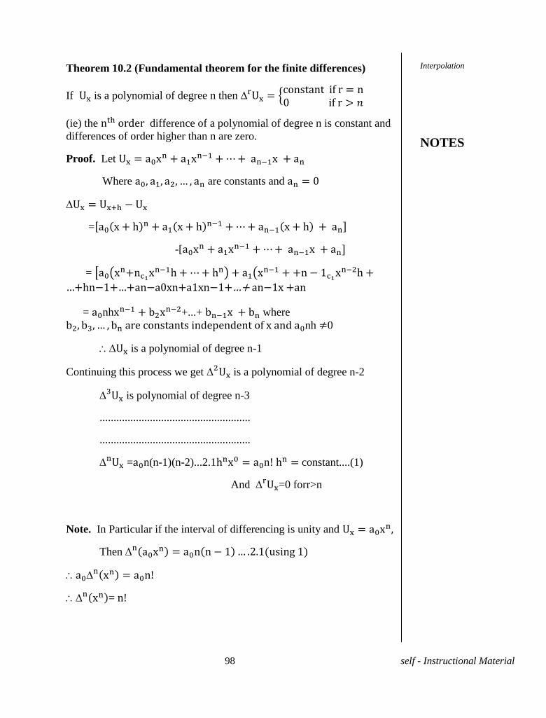
98 self - Instructional Material
Theorem 10.2 (Fundamental theorem for the finite differences)
If is a polynomial of degree n then
(ie) the difference of a polynomial of degree n is constant and
differences of order higher than n are zero.
Proof. Let
Where are constants and
=
-[
=
h an a0xn+a1x + a x +an
= nh +...+
where
nh 0
is a polynomial of degree n-1
Continuing this process we get is a polynomial of degree n-2
is polynomial of degree n-3
......................................................
......................................................
= n(n-1)(n-2)...2.1 n! constant....(1)
And =0 forr>n
Note. In Particular if the interval of differencing is unity and
Then
=
Interpolation
NOTES
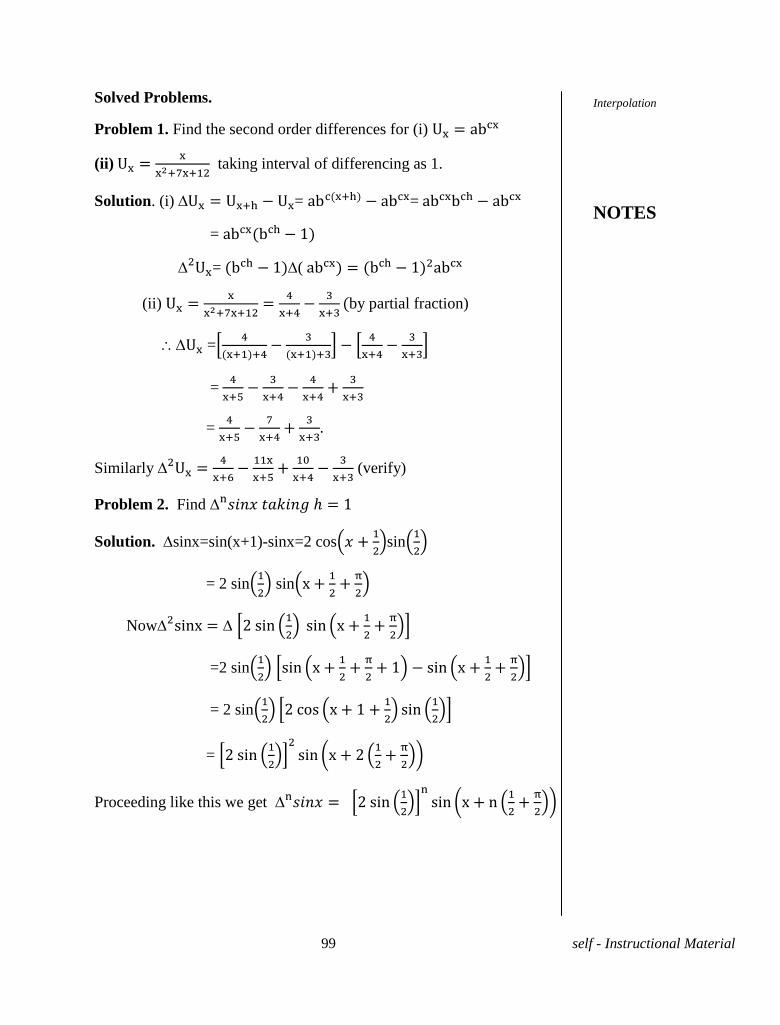
99 self - Instructional Material
Solved Problems.
Problem 1. Find the second order differences for (i)
(ii)
taking interval of differencing as 1.
Solution. (i) = =
=
= (
(ii)
by partial fraction)
=
=
=
Similarly
(verify)
Problem 2. Find ℎ
Solution. sinx=sin(x+1)-sinx=2 cos
sin
= 2 sin
sin
Now
=2 sin
= 2 sin
=
Proceeding like this we get
Interpolation
NOTES
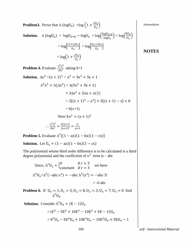
100 self - Instructional Material
Problem3. Prove that (log =log
Solution. (log = log = log
= log
= log
= log
= log
Problem 4. Evaluate.
taking h=1
Solution. =
= (
= 3
= 3
= 6(x+1)
Now E
Problem 5. Evaluate
Solution. Let
The polynomial whose third order difference is to be calculated is a third
degree polynomial and the coefficient of term is – abc
Since,
we have
=
= -6 abc
Problem 6. If find
Solution. Consider
= (
=
Interpolation
NOTES
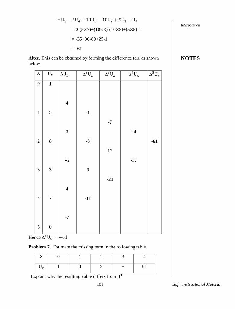
101 self - Instructional Material
=
= 0-(5×7)+(10×3)-(10×8)+(5×5)-1
= -35+30-80+25-1
= -61
Alter. This can be obtained by forming the difference tale as shown
below.
X
0
1
2
3
4
5
1
5
8
3
7
0
4
3
-5
4
-7
-1
-8
9
-11
-7
17
-20
24
-37
-61
Hence
Problem 7. Estimate the missing term in the following table.
X 0 1 2 3 4
1 3 9 - 81
Explain why the resulting value differs from
Interpolation
NOTES
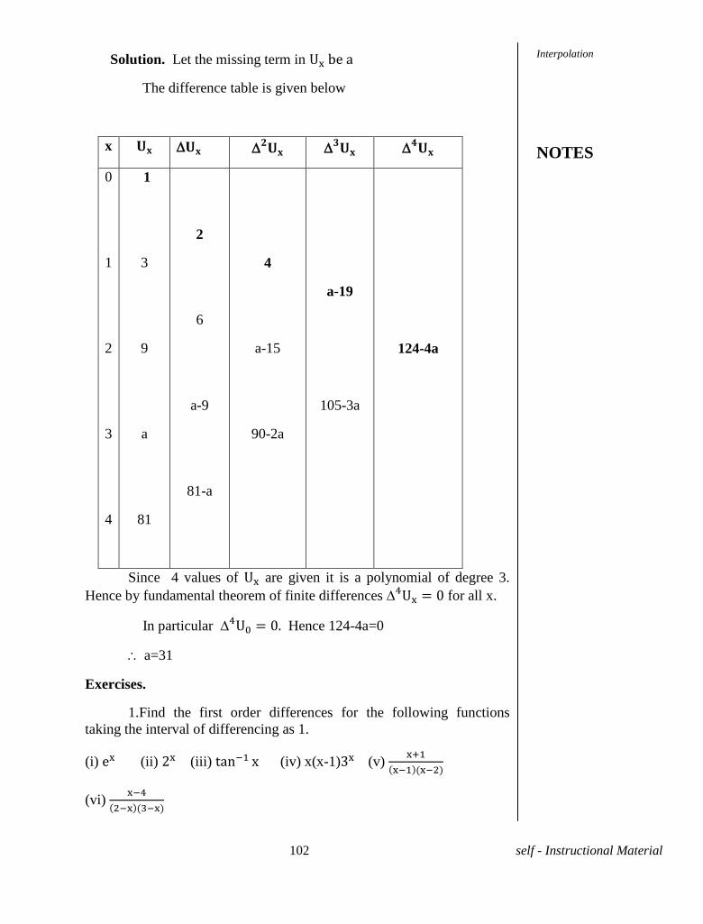
102 self - Instructional Material
Solution. Let the missing term in
The difference table is given below
x
0
1
2
3
4
1
3
9
a
81
2
6
a-9
81-a
4
a-15
90-2a
a-19
105-3a
124-4a
Since 4 values of are given it is a polynomial of degree 3.
Hence by fundamental theorem of finite differences for all x.
In particular Hence 124-4a=0
a=31
Exercises.
1.Find the first order differences for the following functions
taking the interval of differencing as 1.
(i) (ii) (iii) (iv) x(x-1) (v)
(vi)
Interpolation
NOTES
103 self - Instructional Material
2.Prove that tan cx =
c being constant.
3. Prove that (i) ( =
(ii)
=
4.If =2 find taking the interval of
differencing as unity.
5. Show that =6a where If = a and
h is the interval of differencing.
6. Evaluate (i) taking h as interval of differencing.
(ii) taking h=1.
(iii) taking
h=1.
7.Form the difference table for the following data
(i)
x 1 2 3 4 5
2 7 8 11 8
10.3 NEWTON,S FORMULA
Consider the function y =f(x). Let f( f(
f( The replacement of f(x) by a simple function (x) which also
assumes the values at the points is the basic
principle of interpolation. (x) is called a formula for interpolation and
we say that (x) represents f(x). If (x) is a polynomial of degree n then
(x) is called an interpolating polynomial. The existence of an
interpolating polynomial is supposed by Weierstrass; approximation
theorem which asserts that every continuous function on a closed interval
can be approximated by a polynomial.
We now describe Newton –Gregory formula for
constructing a n interpolating polynomial.
Theorem 10.3 (Newton’s –Gregory Interpolating formula for equal
Intervals)
Let be the values of the function at the points a,
a+h, a+2h, .....,a+nh, which are of equal interval of difference.
Interpolation
NOTES
104 self - Instructional Material
Then
+(x-a)(x-a-h)....(x-a- h)
Proof. Let (x) be an interpolating polynomial of degree n which
represents in a x a+nh. Then (x) may be written in the form
(x) =
+.....
+ h) ............(1)
By definition of interpolating polynomial we have
Putting x=a, in(1) we get
Putting x=a+h in (1) we get
=
Putting x =a+2h in (1) we get
=
=
=
(refer example in 2.1)
Similarly substituting x=a+3h, ......, a+ h we get
,.........., =
Substituting these values in (1) we get
(x)=
+(x-a)(x-a-h)....(x-a- h)
Since (x) is the interpolating polynomial which represents the
function (x) can be written as
Interpolation
NOTES
105 self - Instructional Material
+(x-a)(x-a-h)....(x-a- h)
The above formula is known as Newton –Gregory formula for
forward interpolation.
Corollary 1. If we take
=r so that x =a+rh then the Newton –Gregory
formula for forward interpolation reduces to
(a+rh)=
+
Note. Since (x) is the interpolating polynomial which represents the
function (a+rh) can be written as Hence Newton Gregory
formula for forward interpolation becomes,
=
+
Corollary 2. The formula given in cor 1. Can also be used to
extrapolate in the interval (a-h, a)
New ’s Gre ry f rmu a for forward interpolation cannot be
used for interpolating a value of near the end of the given data. To get
a formula for this purpose we can write the interpolating polynomial (x)
of degree n which represent in a+nh x a as
(x)= )+ )(x- )+....+
)(x- ).....(x-
As in the proof of theorem 10.3 we can find
n=0,1,2, ..., n
Thus,
+nUa+nhn!hn a+nh a+h
This is known as Newton’s formula for backward
interpolation.
Taking
-r we get x=a+nh+rh
Further using ,
h=(a+nh)=[a+(n-1)h], 2h=(a+nh)-[a+n-2)h] etc.
Interpolation
NOTES
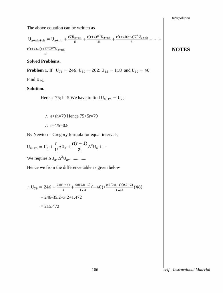
106 self - Instructional Material
The above equation can be written as
Solved Problems.
Problem 1. If ; and
Find
Solution.
Here a=75; h=5 We have to find
a+rh=79 Hence 75+5r=79
r=4/5=0.8
By Newton – Gregory formula for equal intervals,
We require ,...............
Hence we from the difference table as given below
+
= 246-35.2+3.2+1.472
= 215.472
Interpolation
NOTES
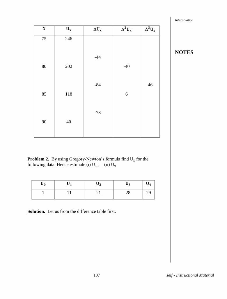
107 self - Instructional Material
X
75
80
85
90
246
202
118
40
-44
-84
-78
-40
6
46
Problem 2. By using Gregory-New ’s f rmu f d for the
following data. Hence estimate (i) (ii)
1 11 21 28 29
Solution. Let us from the difference table first.
Interpolation
NOTES
108 self - Instructional Material
X
0
1
2
3
4
1
11
21
28
29
10
10
7
1
0
-3
-6
-3
-3
0
Here the third order differences are constant and hence the
required function is a polynomial of degree 3. In this case we use the
formula.
Here a=0 and h=1
= 1+10x-
Interpolation
NOTES
109 self - Instructional Material
=
=
(i)
=
= 16.188
(ii)
9 9 9
=
9
Problem 3. Population was recorded as follows in village.
Year 1941 1951 1961 1971 1981 1991
Population 2500 2800 3200 3700 4350 5225
Estimate the population for the year 1945.
Interpolation
NOTES
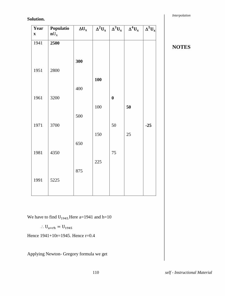
110 self - Instructional Material
Solution.
Year
x
Populatio
n
1941
1951
1961
1971
1981
1991
2500
2800
3200
3700
4350
5225
300
400
500
650
875
100
100
150
225
0
50
75
50
25
-25
We have to find Here a=1941 and h=10
Hence 1941+10r=1945. Hence r=0.4
Applying Newton- Gregory formula we get
Interpolation
NOTES
111 self - Instructional Material
= 2500+120-12-2.08+0.75
= 2606.67
Exercises.
1.If 9 Find
2. Estimate the expectation of life at the age of 16 years from the
following data.
Age in Years 10 15 20 25 30 35
Expectation of life in
Years
35.4 32.3 29.2 26 32.2 20.4
3.If =0.6990; =1; =1.161; and
=1.3010 find
4.Given that sin sin
Sin 9 sin Find sin
5.From the following table find
x 0 6 12 18
23.1234 23.7234 24.6834 26.1330
10.4 LAGRANGE’S FORMULA
Newton-Gregory formula can be used for interpolation only when
we know the values of at points in equal intervals. The following
formula due to the French Mathematician Lagrange can be used when
we know the values of at points which are not at equal intervals. This
formula also enables us to determine the form of the function .
Interpolation
NOTES
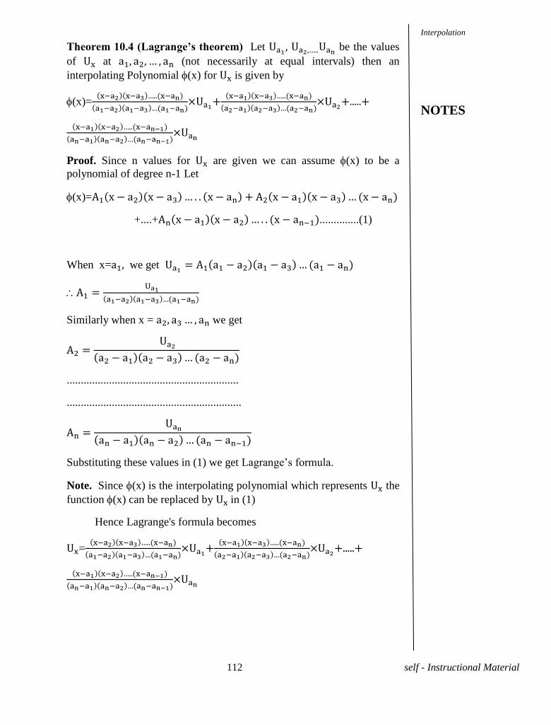
112 self - Instructional Material
Theorem 10.4 (Lagrange’s theorem) Let be the values
of at (not necessarily at equal intervals) then an
interpolating Polynomial (x) for is given by
(x)=
× +
× +.....+
×
Proof. Since n values for are given we can assume (x) to be a
polynomial of degree n-1 Let
(x)=
+....+ ..............(1)
When x= we get
Similarly when x = we get
.............................................................
..............................................................
Substituting these values in (1) we get L r e’s f rmu .
Note. Since (x) is the interpolating polynomial which represents the
function (x) can be replaced by in (1)
Hence Lagrange's formula becomes
=
× +
× +.....+
×
Interpolation
NOTES
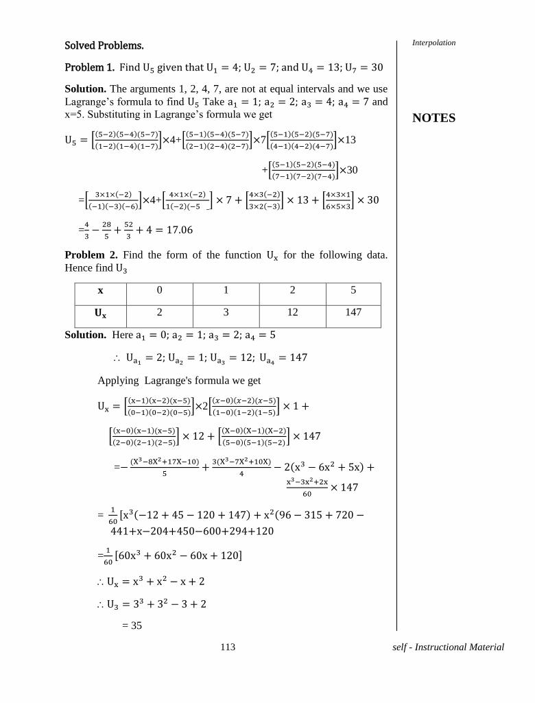
113 self - Instructional Material
Solved Problems.
Problem 1. Find given that ; and
Solution. The arguments 1, 2, 4, 7, are not at equal intervals and we use
L r e’s f rmu f d Take and
x=5. Subs u L r e’s f rmu we e
×4+
×7
×13
+
×30
=
×4+
=
Problem 2. Find the form of the function for the following data.
Hence find
x 0 1 2 5
2 3 12 147
Solution. Here
Applying Lagrange's formula we get
×2
=
=
9
441+x 9 +120
=
= 35
Interpolation
NOTES
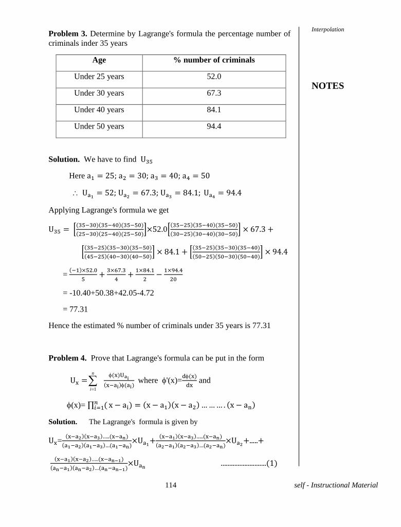
114 self - Instructional Material
Problem 3. Determine by Lagrange's formula the percentage number of
criminals inder 35 years
Age % number of criminals
Under 25 years 52.0
Under 30 years 67.3
Under 40 years 84.1
Under 50 years 94.4
Solution. We have to find
Here
9
Applying Lagrange's formula we get
×52.0
9
=
= -10.40+50.38+42.05-4.72
= 77.31
Hence the estimated % number of criminals under 35 years is 77.31
Problem 4. Prove that Lagrange's formula can be put in the form
1
n
i
where '(x)=
and
(x)=
Solution. The Lagrange's formula is given by
=
× +
× +.....+
× ...........................(1)
Interpolation
NOTES
115 self - Instructional Material
Now (x)= ...........................(2)
log (x)= 1
n
i
log (
Differentiating w.r.t. x we get
Differentiating w.r.t. x we get
=
1
n
i
1
n
i
1
n
i
=
+......+
=
..................................................................
..................................................................
=
Substituting these values in (1) and using (2) we get
+
+
= 1
n
i
Exercises.
1.The following table gives the normal weight of a baby during
first 6 months of life.
Age in month 0 2 3 5 6
Weight in lbs 5 7 8 10 12
Interpolation
NOTES
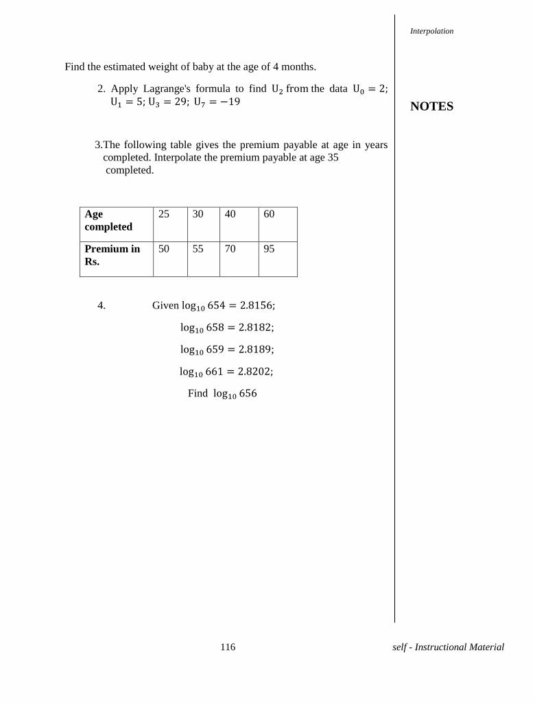
116 self - Instructional Material
Find the estimated weight of baby at the age of 4 months.
2. Apply Lagrange's formula to find the data 9 9
3.The following table gives the premium payable at age in years
completed. Interpolate the premium payable at age 35
completed.
Age
completed
25 30 40 60
Premium in
Rs.
50 55 70 95
4. Given
;
9 9;
Find
Interpolation
NOTES
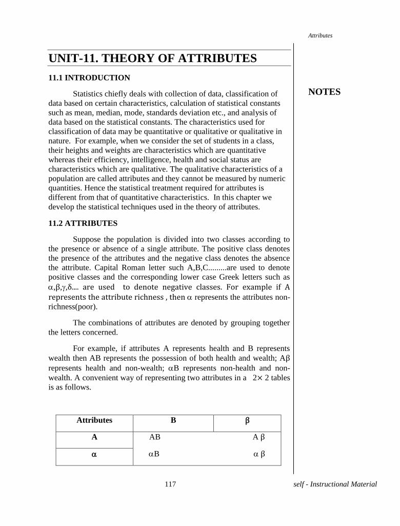
117 self - Instructional Material
UNIT-11. THEORY OF ATTRIBUTES
11.1 INTRODUCTION
Statistics chiefly deals with collection of data, classification of
data based on certain characteristics, calculation of statistical constants
such as mean, median, mode, standards deviation etc., and analysis of
data based on the statistical constants. The characteristics used for
classification of data may be quantitative or qualitative or qualitative in
nature. For example, when we consider the set of students in a class,
their heights and weights are characteristics which are quantitative
whereas their efficiency, intelligence, health and social status are
characteristics which are qualitative. The qualitative characteristics of a
population are called attributes and they cannot be measured by numeric
quantities. Hence the statistical treatment required for attributes is
different from that of quantitative characteristics. In this chapter we
develop the statistical techniques used in the theory of attributes.
11.2 ATTRIBUTES
Suppose the population is divided into two classes according to
the presence or absence of a single attribute. The positive class denotes
the presence of the attributes and the negative class denotes the absence
the attribute. Capital Roman letter such A,B,C.........are used to denote
positive classes and the corresponding lower case Greek letters such as
, , ,δ F represents the attribute richness , then represents the attributes non-
richness(poor).
The combinations of attributes are denoted by grouping together
the letters concerned.
For example, if attributes A represents health and B represents
wealth then AB represents the possession of both health and wealth; A
represents health and non-wealth; B represents non-health and non-
wealth. A convenient way of representing two attributes in a 2 2 tables
is as follows.
Attributes B
A AB A
B
Attributes
NOTES
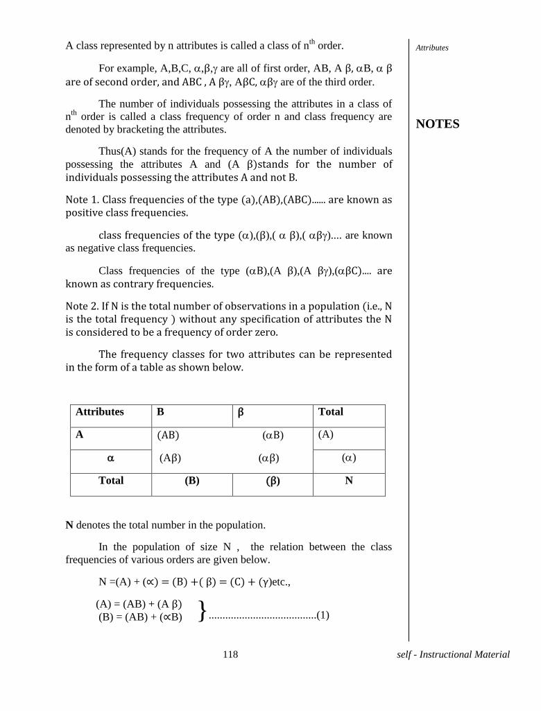
118 self - Instructional Material
A class represented by n attributes is called a class of nth
order.
For example, A,B,C, , , are all of first order, AB, A B, are of second order, and ABC , A , A C are of the third order.
The number of individuals possessing the attributes in a class of
nth
order is called a class frequency of order n and class frequency are
denoted by bracketing the attributes.
Thus(A) stands for the frequency of A the number of individuals
possessing the attributes A and (A stands for the number of individuals possessing the attributes A and not B.
Note 1. Class frequencies of the type (a),(AB),(ABC)...... are known as positive class frequencies.
class frequencies of the type (),( ),( ),( ).... are known
as negative class frequencies.
Class frequencies of the type (B),(A ),(A ),( C known as contrary frequencies.
Note 2. If N is the total number of observations in a population (i.e., N is the total frequency ) without any specification of attributes the N is considered to be a frequency of order zero.
The frequency classes for two attributes can be represented in the form of a table as shown below.
Attributes B Total
A (AB) (B)
(A ) ( )
(A)
()
Total (B) ) N
N denotes the total number in the population.
In the population of size N , the relation between the class
frequencies of various orders are given below.
N =(A) + (∝ C )etc.,
(A) = (AB) + (A (B) = (AB) + (∝B)
}.......................................(1)
Attributes
NOTES
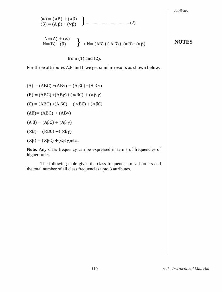
119 self - Instructional Material
(∝ ∝B) + (∝ (A + (∝
∝ N=(B) => N= (AB)+( A (∝B)+ (∝
from (1) and (2).
For three attributes A,B and C we get similar results as shown below.
(A) = (ABC) +(AB C
(B) = (ABC) +(AB ∝ C ∝
(C) = (ABC) +(A C ∝ C ∝ C
(AB)= (ABC) + (AB
(A C
∝ ∝ C +( ∝
∝ ∝ C ∝
Note. Any class frequency can be expressed in terms of frequencies of
higher order.
The following table gives the class frequencies of all orders and
the total number of all class frequencies upto 3 attributes.
}.......................................(2)
}
Attributes
NOTES
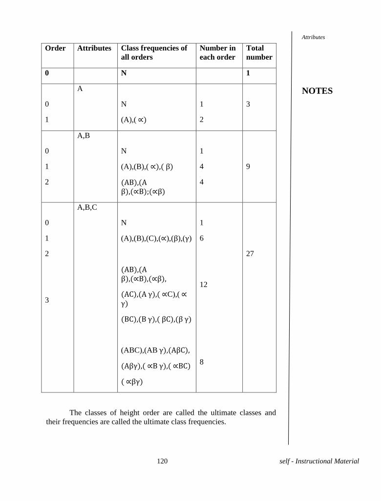
120 self - Instructional Material
Order Attributes Class frequencies of
all orders
Number in
each order
Total
number
0 N 1
0
1
A
N
(A),( ∝
1
2
3
0
1
2
A,B
N
(A),(B),( ∝
(AB),(A ∝ ∝
1
4
4
9
0
1
2
3
A,B,C
N
(A),(B),(C),(∝),( ),( )
(AB),(A ∝ ∝
C ∝C),( ∝
C C
(ABC),(AB C
∝ ∝ C
∝
1
6
12
8
27
The classes of height order are called the ultimate classes and
their frequencies are called the ultimate class frequencies.
Attributes
NOTES
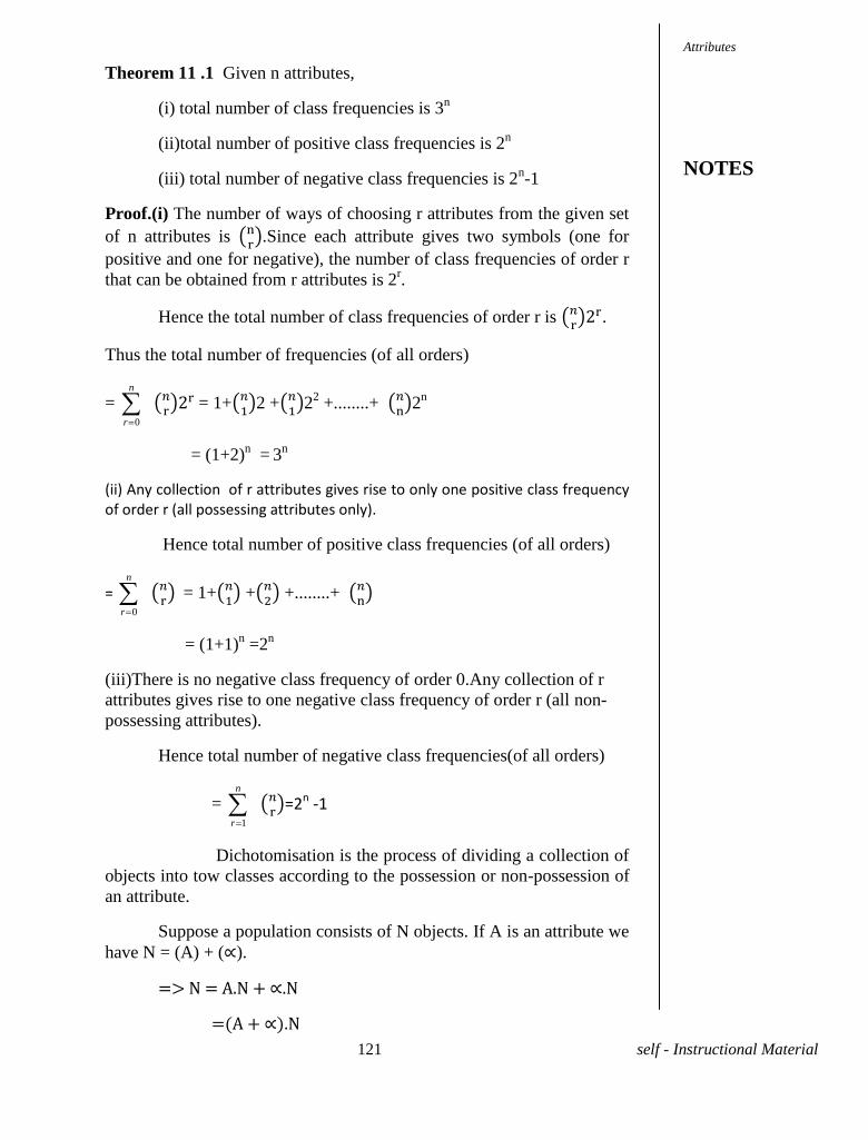
121 self - Instructional Material
Theorem 11 .1 Given n attributes,
(i) total number of class frequencies is 3n
(ii)total number of positive class frequencies is 2n
(iii) total number of negative class frequencies is 2n-1
Proof.(i) The number of ways of choosing r attributes from the given set
of n attributes is .Since each attribute gives two symbols (one for
positive and one for negative), the number of class frequencies of order r
that can be obtained from r attributes is 2r.
Hence the total number of class frequencies of order r is .
Thus the total number of frequencies (of all orders)
= 0
n
r
= 1+
2 +
22
+........+ 2n
= (1+2)
n =
3
n
(ii) Any collection of r attributes gives rise to only one positive class frequency of order r (all possessing attributes only).
Hence total number of positive class frequencies (of all orders)
= 0
n
r
= 1+
+
+........+
= (1+1)n =2
n
(iii)There is no negative class frequency of order 0.Any collection of r
attributes gives rise to one negative class frequency of order r (all non-
possessing attributes).
Hence total number of negative class frequencies(of all orders)
= 1
n
r
=2n -1
Dichotomisation is the process of dividing a collection of
objects into tow classes according to the possession or non-possession of
an attribute.
Suppose a population consists of N objects. If A is an attribute we
have N = (A) + (∝).
∝
∝
Attributes
NOTES
122 self - Instructional Material
∝
Thus in symbolic expression A can be replaced by 1 - ∝ ∝ by 1 - A . This concept is useful to express any class frequency in terms of higher order class frequencies and ultimately in terms of ultimate class frequencies examples 1, and 2 below). Also it is useful to express positive class frequencies (negative class frequencies ) in terms of negative class frequencies (positive class frequencies)(refer examples 3,4, and 5 below).
Examples
1. (AB) = C
Consi - C).N
= AB . N - ABC . N
=(AB) - (ABC)
C
2. If there are two attributes A and B we have
∝
Hence N ∝ ∝ ∝
and N = (B) + ( ∝ ∝
If there are three attributes A,B,C we have
∝
∝ ∝
N C C ∝ C
(∝ ∝ C ∝
3.Consider two attributes A and B.
∝ ∝ -A)(1-B).N
=(1-A-B+AB)
N = N-A.N-B.N+AB.N
= N-(A) - (B) + (AB)
Here negative class frequency has been expressed in terms of positive class frequencies.
Attributes
NOTES
123 self - Instructional Material
4. (AB) = AB.N
(1 -∝ - -∝- -∝
= N - ∝ - ∝ - (∝) - ( ) + (∝ )
Here positive class frequency has been expressed in terms of
negative class frequencies.
5.(∝ ∝ .N = (1 - A)(1 - B)(1 - C).N
= N - A.N - B.N - C.N + AB.N+ AC.N+BC.N - ABC.N
=N - (A) - (B) - (C) + (AB) + (AC) +(BC) - (ABC)
Note. N = (A) + (B) + (C) - (AB) - (BC) -(AC) + (ABC) + (∝ )
Solved problems.
Problem1. Given (A) = 30; (B) =25; (∝ ∝
find ∝
Solution. (i) ∝
(ii) ( - (B)=60-25 = 35
(iii)(AB) = AB.N = (1 - ∝ -
=N - ∝ - ∝
=60-30-35+20 = 15
(iv) = A(1-B).N =(A) - (AB)
=30-15 = 15
∝ ∝ -A)B.N = (B)-(AB)
=25-15=10
Note. The result can also be got directly by completing the 2 2 contingency table for the attributes A and B
(B) ( )
(A) - - 30
(∝) - 20 30
25 - -
Attributes
NOTES
124 self - Instructional Material
Problem 2. Given the following ultimate class frequency of two
attributes A and B. Find the frequencies of positive and negative class
frequencies and the total number of observations.
(AB) = 975 ; (∝ ∝ 9
Solution. Positive class frequencies are (A) and (B)
(A) = (AB) +(A 9
(B) ∝ 9
q ∝
∝ ∝ ∝ 9
( ) = (A ∝ 9 9
N ∝
Taking N ∝
Note. The results can also be got directly by completing the 2 2 contingency table for the attributes A and B.
Problem 3. Given the following positive class frequencies. Find the remaining class frequencies N = 20; (A) = 9; (B)=12;(C) = 8; (AB)=6;(BC)=4;(CA) = 4;(ABC) = 3
Solution. There are three attributes A,B,C
The total number of class frequencies is 33 = 27
We are given only 8 class frequencies and we have to find the remaining 19 class frequencies. They are
Order 1. (∝ - (A)= 20-9=11
( - (B)= 20-12=8
( - (C)= 20-8=12
Order 2. - B).N = (A) - (AB) = 9 - 6 = 3
∝ - B)B.N = (B) - (AB) = 12 - 6 = 6
∝ - B)B.N = (B) - (AB) = 12 - 6 = 6
A(1 - C).N = (A) - (AC) = 9 - 4 = 5
∝C - A)C = (C) - (AC) = 8 - 4 = 4
Attributes
NOTES
125 self - Instructional Material
- C).N = (B) - (BC) = 12 - 4 = 8
C - B)C.N = (C) - (BC) =8 - 4 =4
∝ - A)(1-B).N = N-(A)-(B)+(AB)
=20-9-12+6 =5
(1 - B)(1-C).N = N-(B)-(C)+(BC)
= 20-12-8+4=4
(∝ (1-A)(A-C).N = N-(A)-(C)+(AC)
=20-9-8+4=7
Order 3. AB(1-C).N = (AB)-(ABC)= 6-3=3
C A(1-B)C.N = (AC)-(ABC)= 4-3=1
-B)(1-C).N = (A)-(AC)-(AB)+(ABC)
=9-4-6+3=2
∝ C -A)BC.N =(BC) - (ABC)
= 4-3=1
∝ (1-A)(1-C) B.N=(B)-(BC)-(AB)+(ABC)
=12-4-6+3 =5.
∝ C (1-A)(1-B)C.N = (C)-(AC)-(BC)+(ABC)
=8-4-4+3=3.
∝ (1-A)(1-B)(1-C).N = N-(A)-(B)- (C)+(AB)+(BC)+(CA)-(ABC)
= 20-9-12-8+6+4+4-3 =2
percentage of tube lights which pass the four tests
=
100
= 92.3 %
Attributes
NOTES
126 self - Instructional Material
Exercise
1. Given the frequencies (A) =1150; (∝
∝ 9 F q number of observations.
2. Given the following ultimate class frequencies. Find the frequencies of the positive and negative classes and the total number of observations.
(AB)=733; ∝ 99 ∝
3.Given the following data. Find the frequencies of (i) the remaining positive classes (ii) ultimate classes
N = 1800; (A)=850; (B) = 780; (C) = 326
C 9 ∝ C C
4. Given The Following Ultimate Class frequencies. Find the frequencies of the positive classes.
C 9 C ∝ C ∝ C
9 ∝ ∝
11.3 CONSISTENCY OF DATA
Consider a population with the attributes A and B . For the data
observed in the same population (AB) cannot be greater than (A). Thus
the figures(A) = 20 and (AB) = 25 are inconsistent. We observe that for
he b ve f ures,(Aβ) = (A) - (AB) = -5, which is negative. This
motivated the following definition.
Definition: A set of class frequencies is said to be consistent if none of
them is negative. Otherwise the given set of class frequencies is said to
be inconsistent.
Since any class frequency can be expressed as the sum of the
class frequencies , it follows that a set of independent class frequency a
consistent if and only if no ultimate class frequency is negative.
We have the following set of criteria for testing the consistency in
the set of single attribute, two attributes and three attributes.
Attributes
NOTES
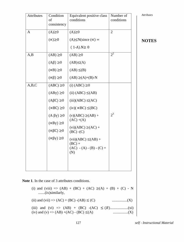
127 self - Instructional Material
Attributes Condition
of
consistency
Equivalent positive class
conditions
Number of
conditions
A (A) 0
(∝ 0
(A) 0
(A) N(since (∝
( 1-A).N
2
A,B (AB) 0
(A 0
(∝B) 0
(∝ 0
(AB) 0
(AB) (A)
(AB) (B)
(AB) (A)+(B)-N
22
A,B,C
(ABC) 0
(AB 0
(A C 0
∝ C 0
(A 0
(∝ 0
(∝ C 0
(∝ 0
(i) (ABC) 0
(ii) (ABC) (AB)
(iii)(ABC) (AC)
(iv)( ∝BC) (BC)
(v)(ABC) (AB) +
(AC) +(A)
(vi)(ABC) (AC) +
(BC) -(C)
(vii)(ABC) (AB) +
(BC) +
(AC) - (A) - (B) - (C) +
(N)
23
Note 1. In the case of 3 attributes conditions.
(i) and (viii) => (AB) + (BC) + (AC) (A) + (B) + (C) - N
.......(ix)similarly,
(ii) and (vii) => (AC) + (BC) -(AB) (C) ................(X)
(iii) and (vi) => (AB) + (BC) -(AC) ...................(xi)
(iv) and (v) => (AB) +(AC) - (BC) (A) ................(X)
Attributes
NOTES
128 self - Instructional Material
Conditions (ix) to (xii) can be used to check the consistency of
the when the class frequency of first and second order alone are know.
Note 2. If the given data are incomplete so that it is not possible to
determined all the class frequencies then the conditions of consistency
can be used determine the limits in which an unknown class frequency
can lie.
Solved problem
Problem 1. Find whether the following data are consistent
N = 600; (A) = 300; (B)=400; (AB) = 50
Solution.We calculate the ultimate class frequencies (∝ ∝
∝ ∝ - A)(1-B).N = N - (A) - (B) + (AB)
=600 - 300 -400 + 50 = -50
S ∝ < 0, the data are inconsistent
Problem 2. Show that there is some error in the following data : 50% people are wealthy ,35 % are wealthy but not healthy,20 % people healthy but not wealthy.
Solution. Taking 'wealth' as A and 'health' as B we get the following data N = 100; ( ∝
∝
∝ ∝ - A)(1-B).N
= N - (A) - (B) + (AB)
But (
∝ 0 + 20 = 70
∝ - 85 - 70 + 50 = -5
∝
Hence there is error in the data.
Problem 3. Of 2000 people consulted 1854 speak Tamil; 1507 speak Hindi;572 speak English;676 speak Tamil and Hindi; 286 speak Tamil and English;270 speak Hindi and English;114 speak Tamil, Hindi and English. Show that the information as it stands is incorrect.
Attributes
NOTES
129 self - Instructional Material
Solution.
Let A C denote the attributes of speaking Tamil, Hindi, English respectively.
Give = 2000; (A) = 1854;(B) = 1507; (C) = 572;
(AB) = 676; (AC) = 286; (BC)= 270; (ABC) = 114
C ∝ ∝ .N
=(1 - A)(1 - B)(1 - C).N
= N - (A) - (B) - (C) - (AB) + (BC) + (AC) - (ABC)
= 2000 - 1854 - 1507 - 572 + 676 + 270 + 286 -114
= - 815
∝ Hence the data are inconsistent
The information is incorrect
Problem 4. Find the limits of (BC) for the following available data;
N = 125; (A) = 48; (B) = 6 C
Solution. First of all we find (AB) and (AC)
(AB) = (A) - - 7 = 41
(AC) = (A) - - 18 = 30
Now, by condition of consistency (ix)
(AB) + (BC) + (AC) (A) +(B) +(C) - N
=> 41 + (BC) + 30 48 + 62 + 45 - 125
(BC) - 41 .............................................................(i)
Also using (xii) , (AB) + (AC) - (BC) (A).
=> (BC) (AB) + (AC) - (A) = 41 + 30 - 48 = 23
(BC) 23 ........................................(ii)
Using (xi),(AB) +(BC) - (AC) (B)
=> (BC) (B) +(AC) - (AB) = 62 + 30 - 41 = 51
Attributes
NOTES
130 self - Instructional Material
(BC) 51 ...........................................(iii) Using (X),(AC) + (BC) - (AB) (C)
=> (BC) (C) + (AB) - (AC) = 45 + 41 - 30 = 56
(BC) 56 ...........................................(iv)
From (i),(ii),(iii) and (iv) we find 23 (BC) 56
Problem 5. Find the greatest and least values of (ABC) (A) = 50;
(B) = 60;
(C) = 80;(AB) = 35; (AC) = 45 and (BC) = 42
solution:
The problem involves 3 attributes and we are given positive class frequencies of first order and second order only.
Using positive class conditions (ii),(iii),(iv) of consistency for 3 attributes
(ABC) (AB) => (ABC) 35 (ABC) (BC) => (ABC) 42 => (ABC) =>35....(1) (ABC) (AC) => (ABC) 45 Using (v),(vi) and (vii)
(ABC) (AB) + (AC) - (A)=> (ABC) 35 + 45 - 50 = 30
(ABC) (AB) + (BC) - (B)=> (ABC) 35 + 42 - 60 = 17
(ABC) (AC) + (BC) - (C)=> (ABC) 45 + 42 - 80 = 7
Thus (ABC) 30 (ABC) 17 .....................(2) (ABC) 7
From (1) and (2) we get 30 (ABC) 35
The least value of (ABC) is 30 and the greatest value of (ABC) is 31
}
}
Attributes
NOTES
131 self - Instructional Material
Exercise
1. Examine the consistency of data when
(i) (A) = 800, (B) = 700,(AB) = 660, N = 1000
(ii) (A) = 600, (B) = 500,(AB) = 50, N = 1000
(iii) N = 2100 (A) = 1000, (B) = 1300,(AB) = 1100
(iv) N = 100 (A) = 45, (B) = 55,(C) = 50(AB) = 15, (BC) = 25, (AC) = 20,
(ABC)= 12
(iv) N = 1800 (A) = 850, (B) = 780,(C) = 326(AB) =250, (BC) = 122,
(AC) =144, (ABC)= 50
2. If (A) = 50, (B) = 60, (C) = 50, (A = 100, find the least and greatest values of (BC)
3. Given that (A) = (B) = (C) =
=50; (AB) = 30,(AC) = 25,
Find the limits which (BC) will lie.
4. If N = 120, (A) = 60,(B) = 90, (C) = 30, (BC) = 15,(AC) = 15,
find the limits between which (AB)must lie.
11.4 INDEPENDENCE AND ASSOCIATION OF DATA
Two attributes A and B are said to be independent if there is same
proportion of A's amongst B's as a amongst ' O q ' ' ∝'
Thus A and B are independent if
=
β
β .........................(i) (or)
=
∝
∝ ...............(ii)
From (i) we get
=
β
β =
β
β =
(AB) =
and (Aβ) =
β
...............(2)
Again from (i) we get 1 -
= 1 -
β
β
Attributes
NOTES
132 self - Instructional Material
=
∝
=
∝
∝
=
∝
=
∝ ∝
=
∝
∝ ) = ∝
........................................(3)
and (∝B) = ∝
.................................................(4)
(1),(2),(3),(4) are all equivalent conditions for independence of the
attributes A and B.
Note. In terms of second order class frequencies we get the condition of
independence as (AB) (∝β) = (Aβ)( ∝B)
For if A and B are independent attributes we have
(AB) (∝β) =
.
∝ β
=
β
β
=(Aβ)( ∝B)
Thus A and B are independent if (AB) (∝β) - (Aβ)( ∝B) = 0 ..........(5)
Association and coefficient of association
If (AB) =
we say that A and B are associated. There are two
possibilities. If(AB) >
we say that A and B are positively
associated and if(AB) <
we say that A and B negatively associated.
N . Le us de e δ = (AB) -
Thus δ = (AB) -
=
[N(AB) - (A)(B)]
=
[{(AB) + (Aβ) + (∝B) + (∝β)} (AB) - {(AB) + (Aβ)} +
(∝B)}]
=
[(AB)( ∝β) - (Aβ)( ∝B)......................................(6)
Note 1. We Know That A and B are independent if δ = 0
A and B are independent if Q = Y = 0
Note 2. If A and B are perfectly associated then (AB) = (A) hence (Aβ)=
0 or (AB) = (B) hence (∝B) = 0. In either Q = 1 = Y
Attributes
NOTES
133 self - Instructional Material
note 3. If A and B are perfectly disassociated then either (AB) = 0 or ∝ = 0 and in this case Q = -1 = Y
Thus we get -1 Q -1
Note. Yule's coefficient Q and the coefficient of colligation Y is related
by the relation Q =
Proof. Let x = ∝
∝ . Hence Y =
=
1+
=
=
=
=
β ∝
∝β
β ∝
∝β
= β β
β β
=Q
From the above relationship between Y and Q we infer the
following
Q=0=> Y=0; Q=-1 => Y=-1 and
Q=1 => Y=1 and conversely.
Solved Problems.
Problem 1. Check whether the attributes A and B are independent given
that (i) (A)=30, (B)=60, (AB)=12, N=150
(ii) (AB)=256, (A )=48, ()=144
Solution. Since the given class frequencies are of first order the
condition for independent is (AB)=
Consider
=
(AB)=
. Hence A and B are independent.
(ii) (A)=(AB)+(A)=256+48=304
Attributes
NOTES
134 self - Instructional Material
(B)= (AB)+()=256+768=1024
()=()+()=768+144=912
()=(A)+()=304+912 =1216
Now,
(AB)=
. Hence A and B are independent.
Aliter. Applying the condition (5) for independence,
(AB)()- (A)(B)=256×144-768×48=36864-36864=0
A and B are independent.
Note. By providing Q=10 also we can conclude A an B are independent.
Problem 2. In a class test in which 135 candidates were examined for
profficiency in Physics and Chemistry, it was discovered that 75 students
failed in Physics, 90 failed in Chemistry and 50 failed in both. Find the
magnititude of association and state if there is any association between
failing in Physics and Chemistry.
Solution. Denoting 'fail in Physics' as A and 'fail in Chemistry' as B we
get
(A)=75, (B)=90, (AB)=50, N=135
The magnititude of association is measured by
Q=
we now get the ultimate class frequencies.
()=N-(A)=135-75=60
()=N-(B)=135-90=45
()=(B)-(AB)=90-50=40
(A)=(A)-(AB)=75-50=25
()=-()=60-40=20
Q=
=0
A and B are independent. Hence failure in Physics and Chemistry are completely independent of each other.
Attributes
NOTES
135 self - Instructional Material
Problem 3. Show whether A and B are independent or positively asociated or negatively associated in the following cases.
(i) N=930, (A)=300, (B)=400, (AB)=230
(ii) (AB)=327, (A)=545, ()=741, ()=235
(iii)(A)=470, (AB)=300, ()=530, ()=150
(iv) (AB)=66, (A)=88, (B)=102, ()=136
Solution. (i)
9
Now, =(AB)-
9 9
Hence >0 Hence A and B are positively associated.
(ii) Q=
=
=
Q<0. Hence A and B are negatively associated.
(iii) N=(A)+()=470+530=1000
(B)=(AB)+(B)=300+150=450
Now,
=(AB)-
=300-2115=-1815
<0. Hence A and B are negatively associated.
(iv) Q=
A and B are independent
Problem 4. Calculate the coefficient of association between intelligence of father and son from the following data.
Intelligent fathers with intelligent sons 200
Intelligent fathers with dull sons 50
Dull fathers with intelligent sons 110
Dull fathers with dull sons 600
Attributes
NOTES
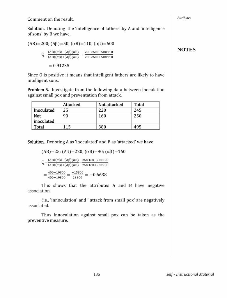
136 self - Instructional Material
Comment on the result.
Solution. Denoting the 'intelligence of fathers' by A and 'intelligence of sons' by B we have.
(AB)=200; (A)=50; (B)=110; ()=600
Q=
= 0.91235
Since Q is positive it means that intelligent fathers are likely to have intelligent sons.
Problem 5. Investigate from the following data between inoculation against small pox and preventation from attack.
Attacked Not attacked Total Inoculated 25 220 245 Not inoculated
90 160 250
Total 115 380 495
Solution. Denoting A as 'inoculated' and B as 'attacked' we have
(AB)=25; (A)=220; (B)=90; ()=160
Q=
=
=
This shows that the attributes A and B have negative association.
(ie., 'innoculation' and ' attack from small pox' are negatively associated.
Thus innoculation against small pox can be taken as the preventive measure.
Attributes
NOTES
137 self - Instructional Material
Exercises. Show whether A and B are independent , positively associated or negatively associated.
1.Show whether A and B are indepentent, positiviely associated or negatively associated.
(i) N=392, (A)=154, (B)=168, (AB)=66
(ii) N=1000, (A)=470, (B)=620, (AB)=320
(iii) (A)=28, (B)=38, (AB)=12, N=60
(iv) (AB)=90; (A)=65; (B)=260; ()=110
(v)(A)=245, ()=285, (AB)=147, ()=190
2. In an examination in Tamil and English 245 of the candidates passed in Tamil, 147 passed in both, 285 failed in Tamil and 190 failed in Tamil but passed in English. Howfar is the knowledge in the two subjects associated?
3. Calculate Yule's coefficient of association between marriage and failure of students
Passed Failed Total Married Unmarried Total
90 260 350
65 110 175
155 370 525
Attributes
NOTES
138 self - Instructional Material
UNIT XII- INDEX NUMBERS
12.1 INDEX NUMBERS
An Index number is a widely used statistical device for
comparing the level of a certain phenomenon with the level of the same
phenomenon at some standard period. For example , we may wish to
compare the price of a food article at a particular period with the price of
the same article at a previous period of time. This Compar4ision can be
expressed as the percentage of ration of the prices in the two periods and
this number serves as a single food-price index number. The comparison
of prices of several food articles at two different periods is usually
expressed as a suitable weighted average of the percentage changes in
these prices. In the calculation of averages, various standard measures of
central tendencies such as Arithmetic mean , Geometric Mean, Harmonic
mean can be used.
In the computation of an index number, if the base year used for
comparison is kept constant throughtout, then it is called fixed base
method. If on the other hand, for every year the previous year is used as
a base for comparison, then the method is called chain base method.
Index numbers can be broadly classified into two types.
(i)Unweighted or simple index number.
(ii)Weighted index number.
Two standard methods of computation are
(A) Aggregate method.
(B) Average of price relatives method
I-A Aggregate Method.
In this method total of current year prices for various
commodities is divided by the total of the base year. In symbols, if
denotes the price of the base year and the price of the current year
where is total of the current year and
is the total of the base year.
This is the simplest method inwhich aggregate of the prices for base
year and current year alone are taken into consideration.
Index Numbers
NOTES
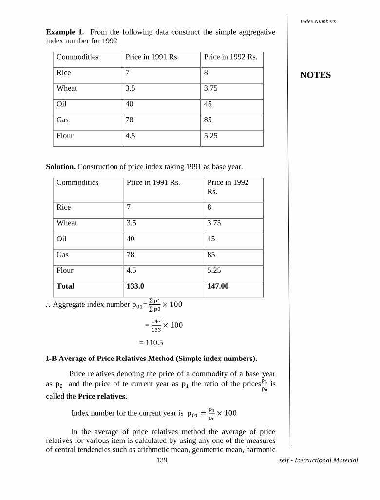
139 self - Instructional Material
Example 1. From the following data construct the simple aggregative
index number for 1992
Commodities Price in 1991 Rs. Price in 1992 Rs.
Rice 7 8
Wheat 3.5 3.75
Oil 40 45
Gas 78 85
Flour 4.5 5.25
Solution. Construction of price index taking 1991 as base year.
Commodities Price in 1991 Rs. Price in 1992
Rs.
Rice 7 8
Wheat 3.5 3.75
Oil 40 45
Gas 78 85
Flour 4.5 5.25
Total 133.0 147.00
Aggregate index number =
=
= 110.5
I-B Average of Price Relatives Method (Simple index numbers).
Price relatives denoting the price of a commodity of a base year
as and the price of te current year as the ratio of the prices
is
called the Price relatives.
Index number for the current year is
In the average of price relatives method the average of price
relatives for various item is calculated by using any one of the measures
of central tendencies such as arithmetic mean, geometric mean, harmonic
Index Numbers
NOTES
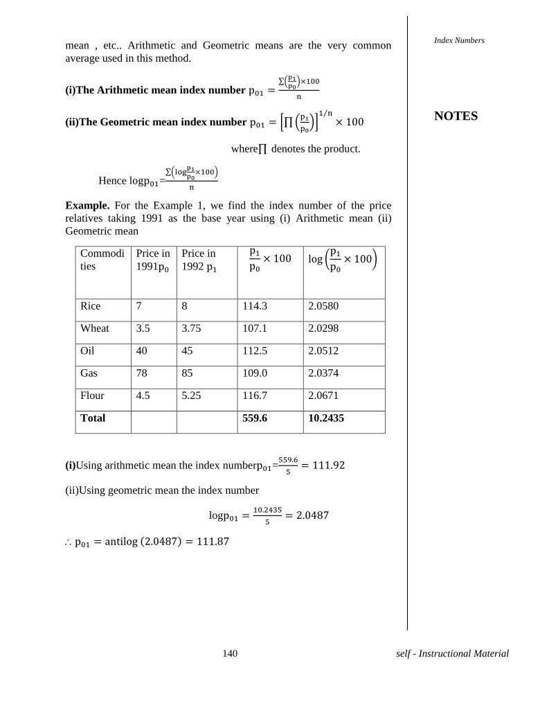
140 self - Instructional Material
mean , etc.. Arithmetic and Geometric means are the very common
average used in this method.
(i)The Arithmetic mean index number
(ii)The Geometric mean index number
where denotes the product.
Hence log =
Example. For the Example 1, we find the index number of the price
relatives taking 1991 as the base year using (i) Arithmetic mean (ii)
Geometric mean
Commodi
ties
Price in
1991
Price in
1992
Rice 7 8 114.3 2.0580
Wheat 3.5 3.75 107.1 2.0298
Oil 40 45 112.5 2.0512
Gas 78 85 109.0 2.0374
Flour 4.5 5.25 116.7 2.0671
Total 559.6 10.2435
(i)Using arithmetic mean the index number =
9
(ii)Using geometric mean the index number
log
Index Numbers
NOTES
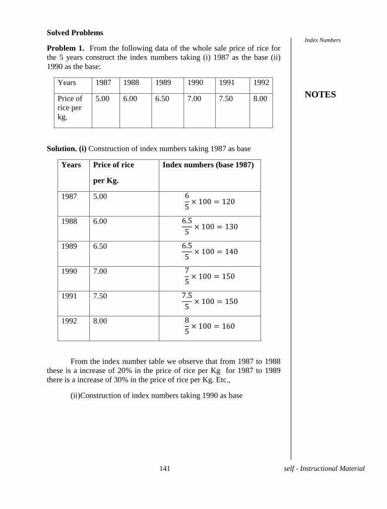
141 self - Instructional Material
Solved Problems
Problem 1. From the following data of the whole sale price of rice for
the 5 years construct the index numbers taking (i) 1987 as the base (ii)
1990 as the base:
Years 1987 1988 1989 1990 1991 1992
Price of
rice per
kg.
5.00 6.00 6.50 7.00 7.50 8.00
Solution. (i) Construction of index numbers taking 1987 as base
Years Price of rice
per Kg.
Index numbers (base 1987)
1987 5.00
1988 6.00
1989 6.50
1990 7.00
1991 7.50
1992 8.00
From the index number table we observe that from 1987 to 1988
these is a increase of 20% in the price of rice per Kg for 1987 to 1989
there is a increase of 30% in the price of rice per Kg. Etc.,
(ii)Construction of index numbers taking 1990 as base
Index Numbers
NOTES
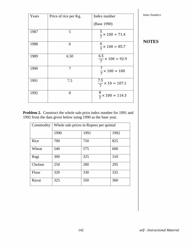
142 self - Instructional Material
Years Price of rice per Kg. Index number
(Base 1990)
1987 5
1988 6
1989 6.50
9 9
1990 7
1991 7.5
1992 8
Problem 2. Construct the whole sale price index number for 1991 and
1992 from the data given below using 1990 as the base year.
Commodity Whole sale prices in Rupees per quintal
1990 1991 1992
Rice 700 750 825
Wheat 540 575 600
Ragi 300 325 310
Cholam 250 280 295
Flour 320 330 335
Ravai 325 350 360
Index Numbers
NOTES
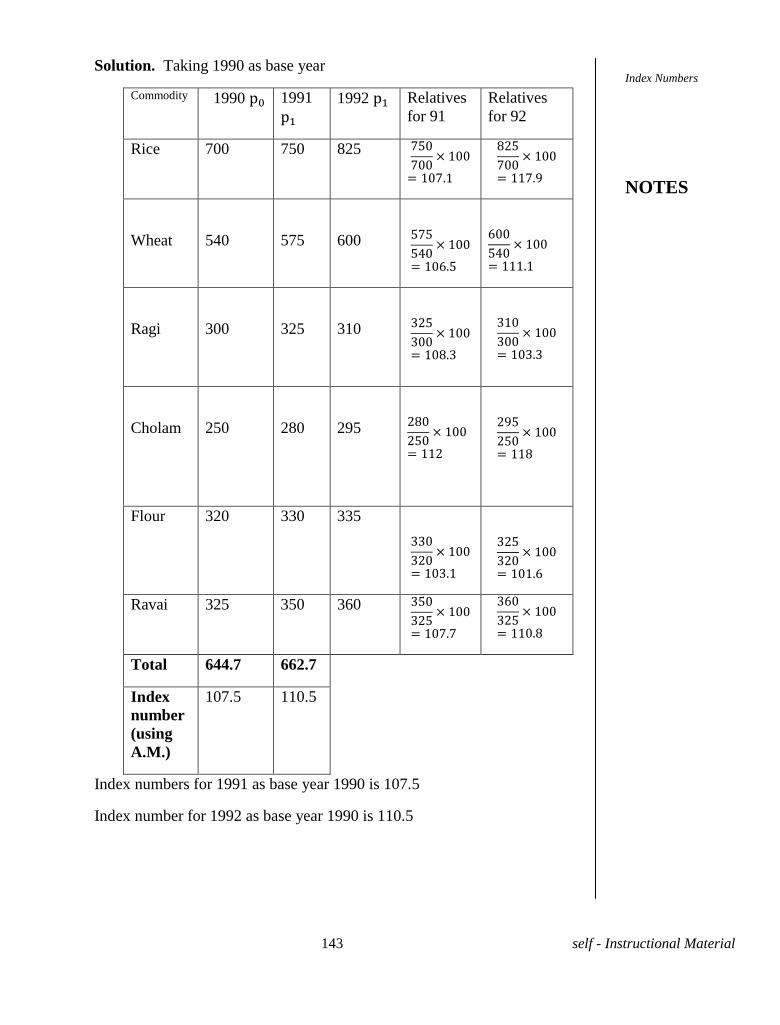
143 self - Instructional Material
Solution. Taking 1990 as base year
Commodity 1990 1991
1992 Relatives
for 91
Relatives
for 92
Rice 700 750 825
9
Wheat
540
575
600
Ragi
300
325
310
Cholam
250
280
295
9
Flour 320 330 335
Ravai 325 350 360
Total 644.7 662.7
Index
number
(using
A.M.)
107.5 110.5
Index numbers for 1991 as base year 1990 is 107.5
Index number for 1992 as base year 1990 is 110.5
Index Numbers
NOTES
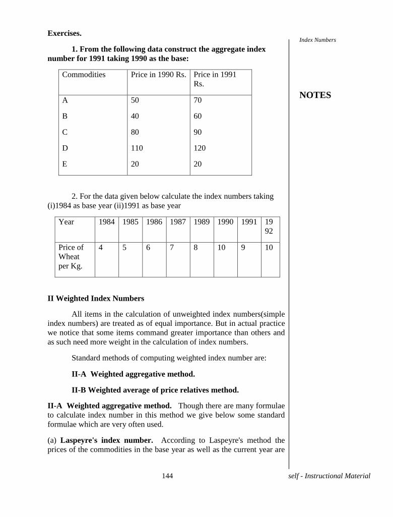
144 self - Instructional Material
Exercises.
1. From the following data construct the aggregate index
number for 1991 taking 1990 as the base:
Commodities Price in 1990 Rs. Price in 1991
Rs.
A
B
C
D
E
50
40
80
110
20
70
60
90
120
20
2. For the data given below calculate the index numbers taking
(i)1984 as base year (ii)1991 as base year
Year 1984 1985 1986 1987 1989 1990 1991 19
92
Price of
Wheat
per Kg.
4 5 6 7 8 10 9 10
II Weighted Index Numbers
All items in the calculation of unweighted index numbers(simple
index numbers) are treated as of equal importance. But in actual practice
we notice that some items command greater importance than others and
as such need more weight in the calculation of index numbers.
Standard methods of computing weighted index number are:
II-A Weighted aggregative method.
II-B Weighted average of price relatives method.
II-A Weighted aggregative method. Though there are many formulae
to calculate index number in this method we give below some standard
formulae which are very often used.
(a) Laspeyre's index number. According to Laspeyre's method the
prices of the commodities in the base year as well as the current year are
Index Numbers
NOTES
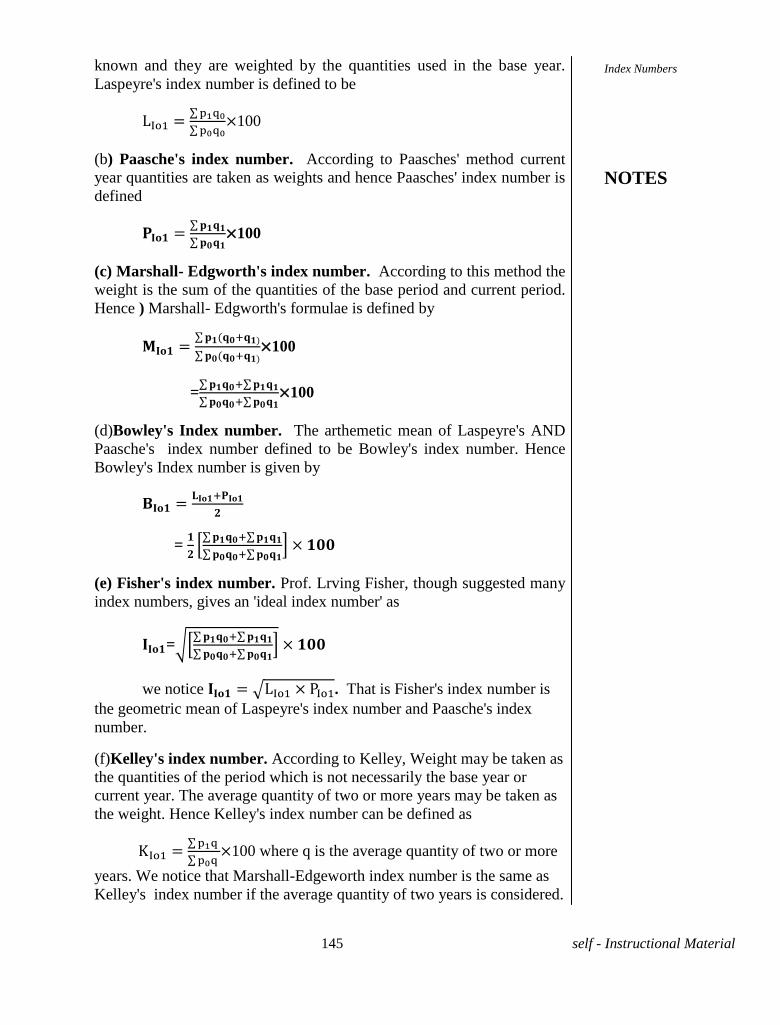
145 self - Instructional Material
known and they are weighted by the quantities used in the base year.
Laspeyre's index number is defined to be
×100
(b) Paasche's index number. According to Paasches' method current
year quantities are taken as weights and hence Paasches' index number is
defined
×100
(c) Marshall- Edgworth's index number. According to this method the
weight is the sum of the quantities of the base period and current period.
Hence ) Marshall- Edgworth's formulae is defined by
×100
=
×100
(d)Bowley's Index number. The arthemetic mean of Laspeyre's AND
Paasche's index number defined to be Bowley's index number. Hence
Bowley's Index number is given by
=
(e) Fisher's index number. Prof. Lrving Fisher, though suggested many
index numbers, gives an 'ideal index number' as
=
we notice . That is Fisher's index number is
the geometric mean of Laspeyre's index number and Paasche's index
number.
(f)Kelley's index number. According to Kelley, Weight may be taken as
the quantities of the period which is not necessarily the base year or
current year. The average quantity of two or more years may be taken as
the weight. Hence Kelley's index number can be defined as
×100 where q is the average quantity of two or more
years. We notice that Marshall-Edgeworth index number is the same as
Kelley's index number if the average quantity of two years is considered.
Index Numbers
NOTES
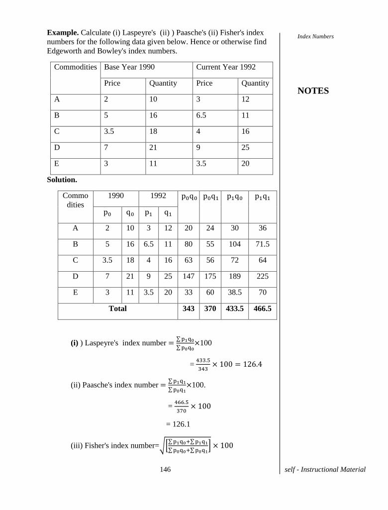
146 self - Instructional Material
Example. Calculate (i) Laspeyre's (ii) ) Paasche's (ii) Fisher's index
numbers for the following data given below. Hence or otherwise find
Edgeworth and Bowley's index numbers.
Commodities Base Year 1990 Current Year 1992
Price Quantity Price Quantity
A 2 10 3 12
B 5 16 6.5 11
C 3.5 18 4 16
D 7 21 9 25
E 3 11 3.5 20
Solution.
Commo
dities
1990 1992 q q q q
q q
A 2 10 3 12 20 24 30 36
B 5 16 6.5 11 80 55 104 71.5
C 3.5 18 4 16 63 56 72 64
D 7 21 9 25 147 175 189 225
E 3 11 3.5 20 33 60 38.5 70
Total 343 370 433.5 466.5
(i) ) Laspeyre's index number
×100
=
(ii) Paasche's index number
×100.
=
= 126.1
(iii) Fisher's index number=
Index Numbers
NOTES
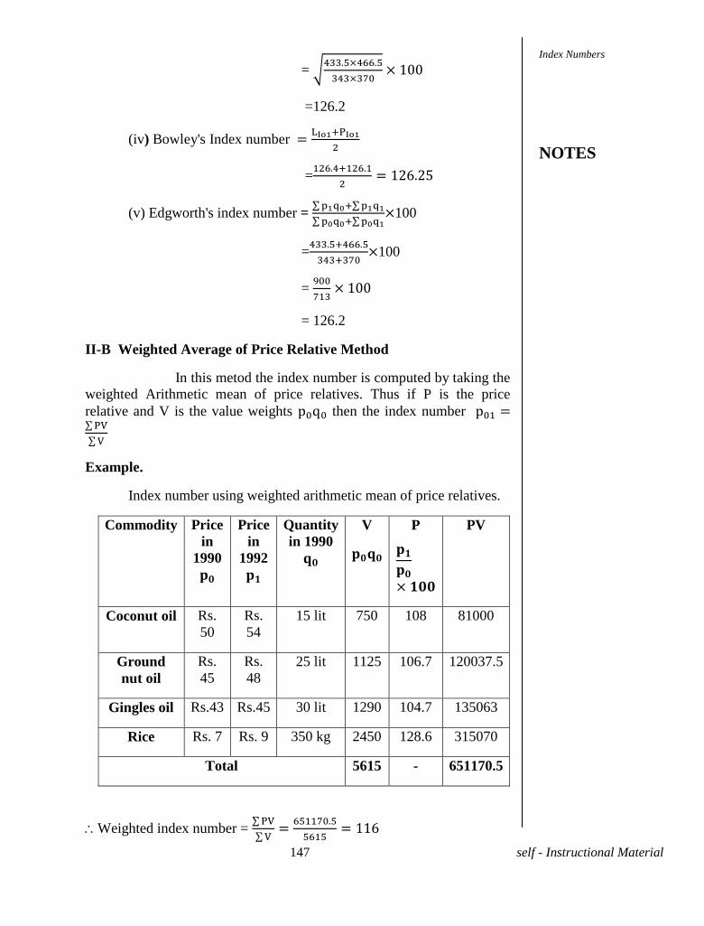
147 self - Instructional Material
=
=126.2
(iv) Bowley's Index number
=
(v) Edgworth's index number =
×100
=
×100
=
= 126.2
II-B Weighted Average of Price Relative Method
In this metod the index number is computed by taking the
weighted Arithmetic mean of price relatives. Thus if P is the price
relative and V is the value weights q then the index number
Example.
Index number using weighted arithmetic mean of price relatives.
Commodity
Price
in
1990
Price
in
1992
Quantity
in 1990
V
P
PV
Coconut oil Rs.
50
Rs.
54
15 lit 750 108 81000
Ground
nut oil
Rs.
45
Rs.
48
25 lit 1125 106.7 120037.5
Gingles oil Rs.43 Rs.45 30 lit 1290 104.7 135063
Rice Rs. 7 Rs. 9 350 kg 2450 128.6 315070
Total 5615 - 651170.5
Weighted index number =
Index Numbers
NOTES
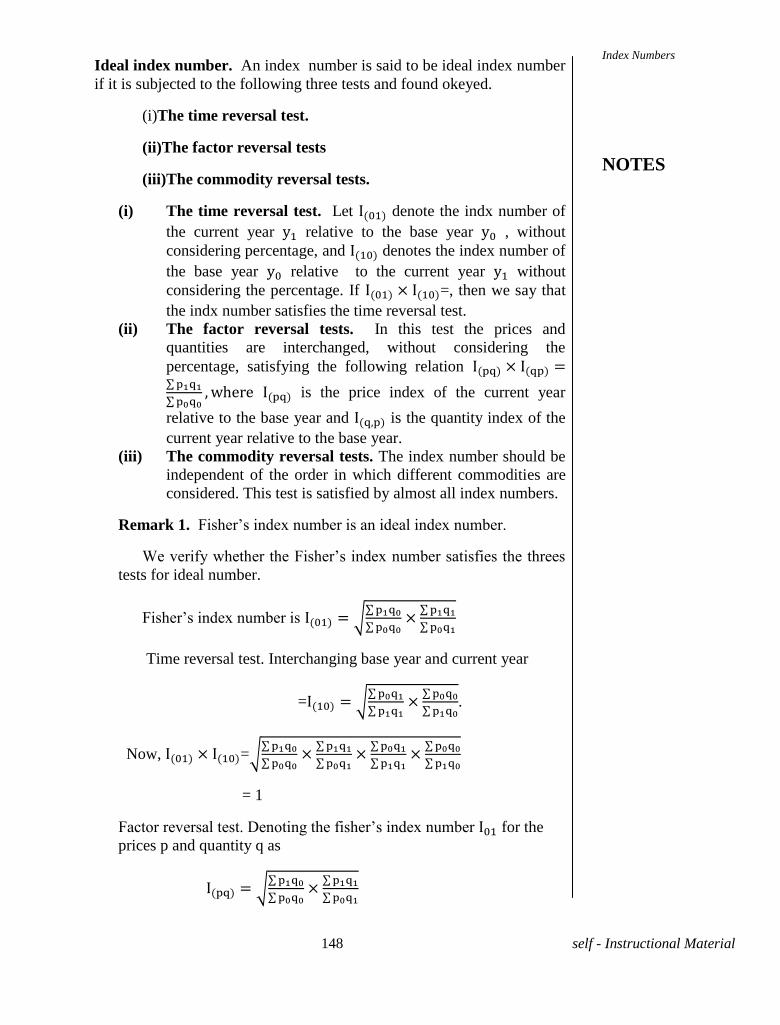
148 self - Instructional Material
Ideal index number. An index number is said to be ideal index number
if it is subjected to the following three tests and found okeyed.
(i)The time reversal test.
(ii)The factor reversal tests
(iii)The commodity reversal tests.
(i) The time reversal test. Let denote the indx number of
the current year relative to the base year , without
considering percentage, and denotes the index number of
the base year relative to the current year without
considering the percentage. If =, then we say that
the indx number satisfies the time reversal test.
(ii) The factor reversal tests. In this test the prices and
quantities are interchanged, without considering the
percentage, satisfying the following relation
is the price index of the current year
relative to the base year and is the quantity index of the
current year relative to the base year.
(iii) The commodity reversal tests. The index number should be
independent of the order in which different commodities are
considered. This test is satisfied by almost all index numbers.
Remark 1. F sher’s dex umber s de dex umber.
We ver fy whe her he F sher’s dex umber s sf es he hrees
tests for ideal number.
F sher’s dex umber s
Time reversal test. Interchanging base year and current year
=
.
Now, =
= 1
F c r revers es . De he f sher’s dex umber for the
prices p and quantity q as
Index Numbers
NOTES
149 self - Instructional Material
Interchanging the prices and quantities in we get
Now,
.
=
Obv us y F sher’s dex umber s sf es he c mm d y revers es .
He ce F sher’s dex umber s de dex umber.
Note. Of he dex umbers def ed e r er F sher’s dex umber s
the only index number which is an ideal index number.
Remark 2. L speyer’s dex umber d es s sfy he me revers
test. ] We have =
and
Now,
He ce L speyre’s dex umber d es s sfy he me revers es
Remark 3. P sche’s dex umber d es s sfy he me revers
test. .(Verify)
Remark 4. L speyre’s d P sche’s dex umber s d s sfy
factor reversal test. .(Verify)
Solved Problems.
Problem 1. C s ruc , w h he he p f d ve be w , F sher’s
index number and shown that it satisfies both the factor reversal test and
time reversal test.
Commodity A B C D
Base year price in
Rupees
5 6 4 3
Base Year quantity in
Quintals
50 40 120 30
Current year price in
Rupees
7 8 5 4
Current year quantity
in Quintals
60 50 110 35
Index Numbers
NOTES
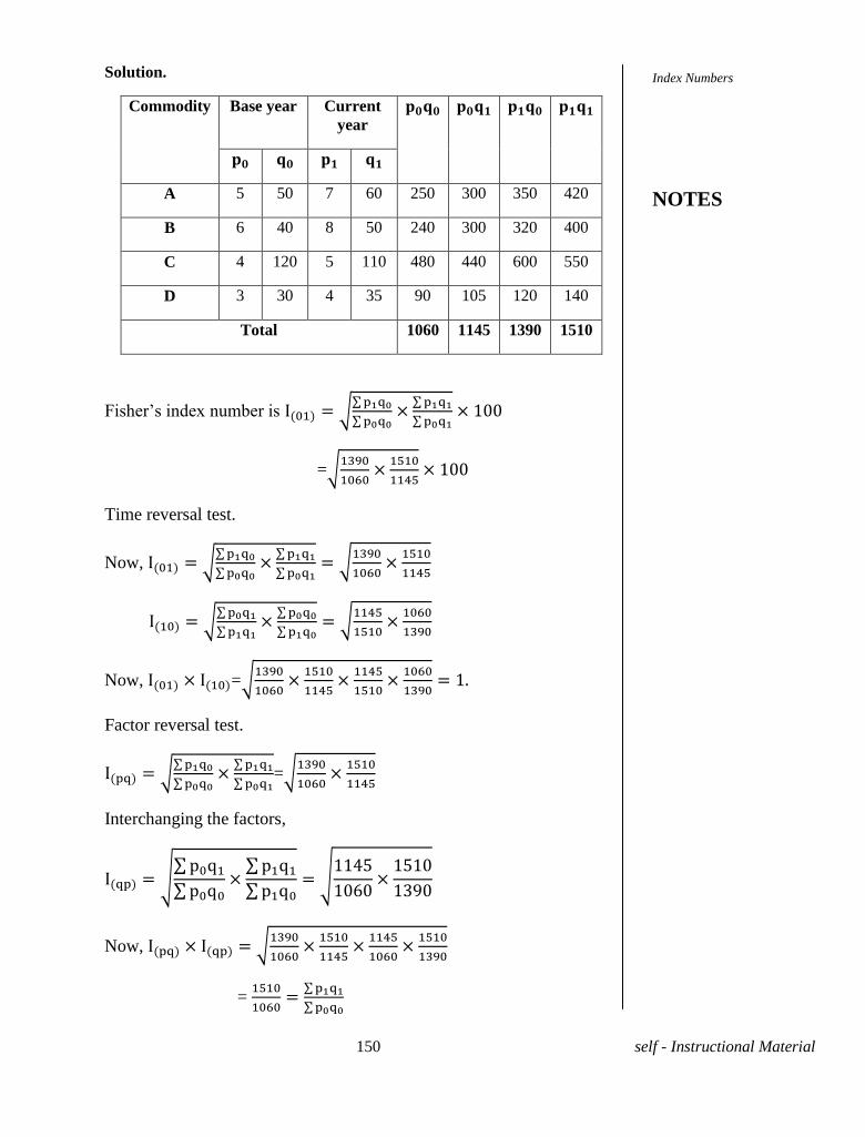
150 self - Instructional Material
Solution.
Commodity Base year Current
year
A 5 50 7 60 250 300 350 420
B 6 40 8 50 240 300 320 400
C 4 120 5 110 480 440 600 550
D 3 30 4 35 90 105 120 140
Total 1060 1145 1390 1510
F sher’s dex umber s
=
Time reversal test.
Now,
Now, =
Factor reversal test.
=
Interchanging the factors,
q q
q q
9
Now,
=
Index Numbers
NOTES
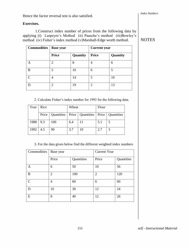
151 self - Instructional Material
Hence the factor reversal test is also satisfied.
Exercises.
1.Construct index number of prices from the following data by
applying (i) L speyre’s Me h d ( ) P sche’s me h d ( )B w ey’s
me h d ( v) F sher’s dex me h d (v)M rsh -Edge worth method.
Commodities Base year Current year
Price Quantity Price Quantity
A 2 8 4 6
B 5 10 6 5
C 4 14 5 10
D 2 19 2 13
2. C cu e F sher’s dex umber f r 1992 f r he f w d .
Year Rice Wheat Flour
Price Quantities Price Quantities Price Quantities
1988 9.3 100 6.4 11 5.1 5
1992 4.5 90 3.7 10 2.7 3
3. For the data given below find the different weighted index numbers
Commodities Base year Current Year
Price Quantities Price Quantities
A 6 50 10 56
B 2 100 2 120
C 4 60 6 60
D 10 30 12 24
E 8 40 12 26
Index Numbers
NOTES
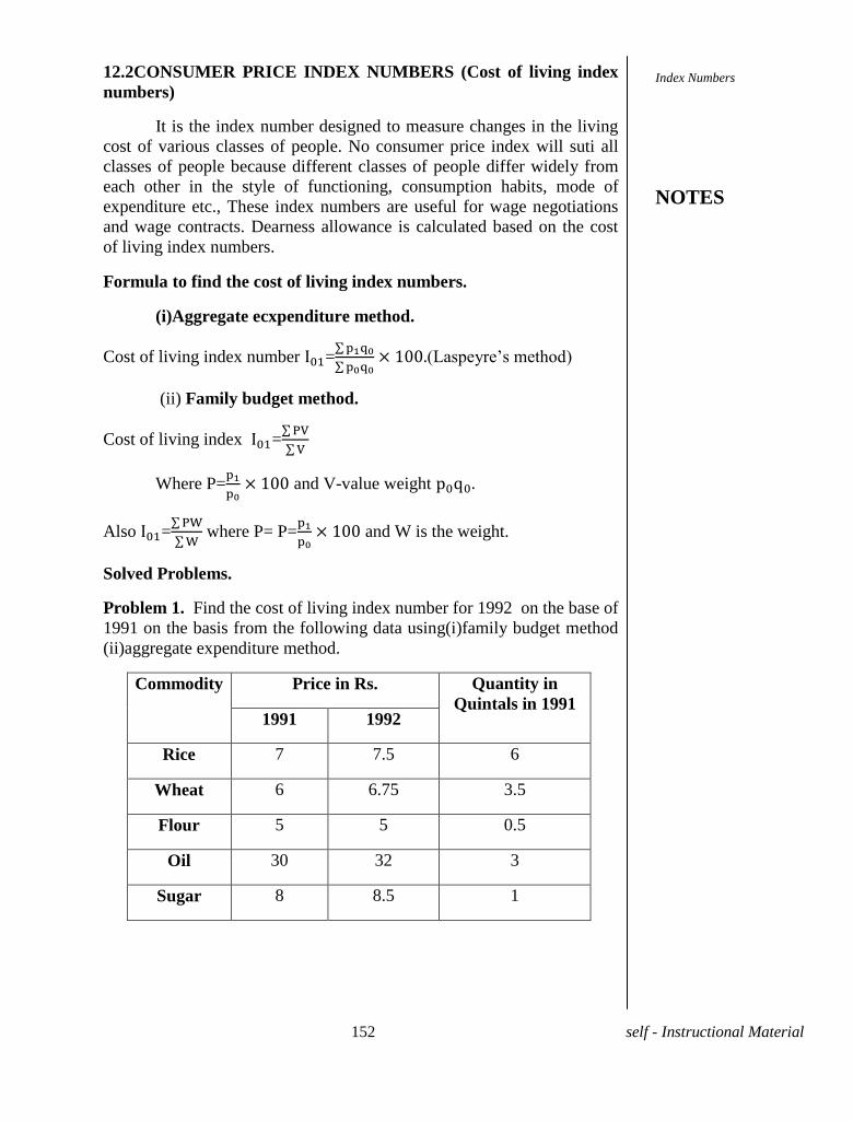
152 self - Instructional Material
12.2CONSUMER PRICE INDEX NUMBERS (Cost of living index
numbers)
It is the index number designed to measure changes in the living
cost of various classes of people. No consumer price index will suti all
classes of people because different classes of people differ widely from
each other in the style of functioning, consumption habits, mode of
expenditure etc., These index numbers are useful for wage negotiations
and wage contracts. Dearness allowance is calculated based on the cost
of living index numbers.
Formula to find the cost of living index numbers.
(i)Aggregate ecxpenditure method.
Cost of living index number =
(L speyre’s me h d)
(ii) Family budget method.
Cost of living index =
Where P=
and V-value weight q
Also =
where P= P=
and W is the weight.
Solved Problems.
Problem 1. Find the cost of living index number for 1992 on the base of
1991 on the basis from the following data using(i)family budget method
(ii)aggregate expenditure method.
Commodity Price in Rs. Quantity in
Quintals in 1991 1991 1992
Rice 7 7.5 6
Wheat 6 6.75 3.5
Flour 5 5 0.5
Oil 30 32 3
Sugar 8 8.5 1
Index Numbers
NOTES
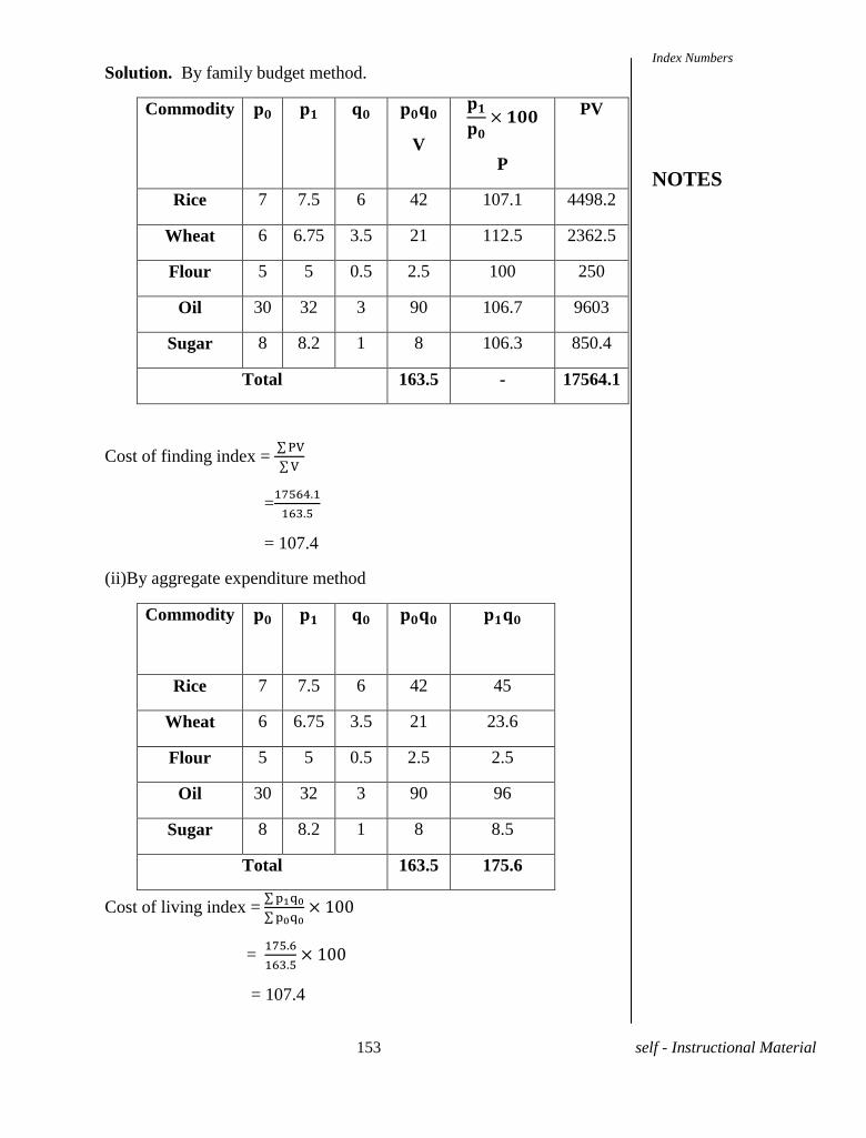
153 self - Instructional Material
Solution. By family budget method.
Commodity
V
P
PV
Rice 7 7.5 6 42 107.1 4498.2
Wheat 6 6.75 3.5 21 112.5 2362.5
Flour 5 5 0.5 2.5 100 250
Oil 30 32 3 90 106.7 9603
Sugar 8 8.2 1 8 106.3 850.4
Total 163.5 - 17564.1
Cost of finding index =
=
= 107.4
(ii)By aggregate expenditure method
Commodity
Rice 7 7.5 6 42 45
Wheat 6 6.75 3.5 21 23.6
Flour 5 5 0.5 2.5 2.5
Oil 30 32 3 90 96
Sugar 8 8.2 1 8 8.5
Total 163.5 175.6
Cost of living index =
=
= 107.4
Index Numbers
NOTES
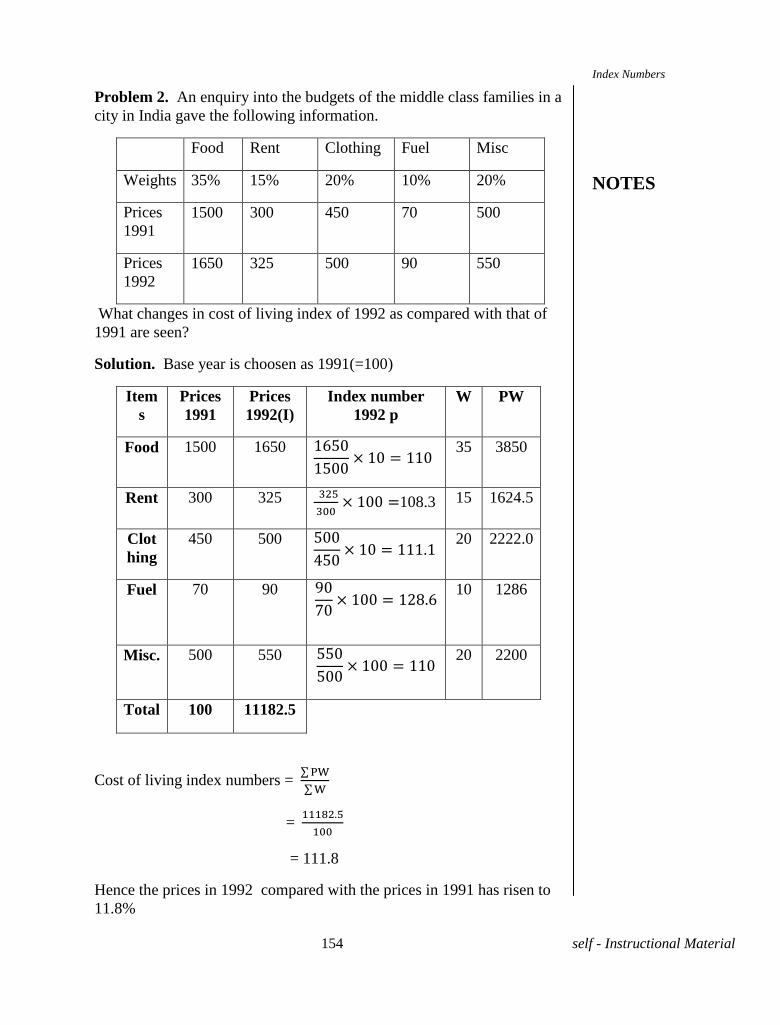
154 self - Instructional Material
Problem 2. An enquiry into the budgets of the middle class families in a
city in India gave the following information.
Food Rent Clothing Fuel Misc
Weights 35% 15% 20% 10% 20%
Prices
1991
1500 300 450 70 500
Prices
1992
1650 325 500 90 550
What changes in cost of living index of 1992 as compared with that of
1991 are seen?
Solution. Base year is choosen as 1991(=100)
Item
s
Prices
1991
Prices
1992(I)
Index number
1992 p
W PW
Food 1500 1650
35 3850
Rent 300 325
108.3 15 1624.5
Clot
hing
450 500
20 2222.0
Fuel 70 90 9
10 1286
Misc. 500 550
20 2200
Total 100 11182.5
Cost of living index numbers =
=
= 111.8
Hence the prices in 1992 compared with the prices in 1991 has risen to
11.8%
Index Numbers
NOTES
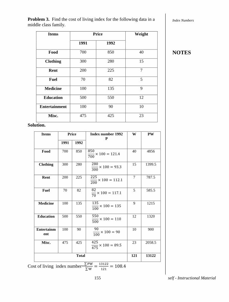
155 self - Instructional Material
Problem 3. Find the cost of living index for the following data in a
middle class family.
Items Price Weight
1991 1992
Food 700 850 40
Clothing 300 280 15
Rent 200 225 7
Fuel 70 82 5
Medicine 100 135 9
Education 500 550 12
Entertainment 100 90 10
Misc. 475 425 23
Solution.
Items Price Index number 1992
P
W PW
1991 1992
Food 700 850
40 4856
Clothing 300 280
9
15 1399.5
Rent 200 225
7 787.5
Fuel 70 82
5 585.5
Medicine 100 135
9 1215
Education 500 550
12 1320
Entertainm
ent
100 90 9
9
10 900
Misc. 475 425
9
23 2058.5
Total 121 13122
Cost of living index number=
Index Numbers
NOTES
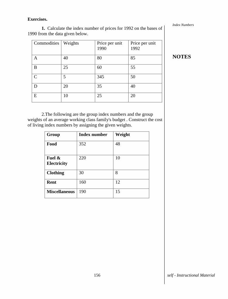
156 self - Instructional Material
Exercises.
1. Calculate the index number of prices for 1992 on the bases of
1990 from the data given below.
Commodities Weights Price per unit
1990
Price per unit
1992
A 40 80 85
B 25 60 55
C 5 345 50
D 20 35 40
E 10 25 20
2.The following are the group index numbers and the group
weights of an average working class family's budget . Construct the cost
of living index numbers by assigning the given weights.
Group Index number Weight
Food 352 48
Fuel &
Electricity
220 10
Clothing 30 8
Rent 160 12
Miscellaneous 190 15
Index Numbers
NOTES
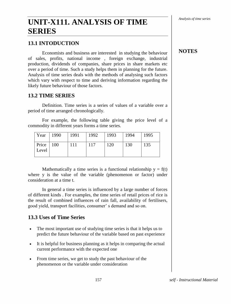
157 self - Instructional Material
UNIT-X111. ANALYSIS OF TIME
SERIES
13.1 INTODUCTION
Economists and business are interested in studying the behaviour
of sales, profits, national income , foreign exchange, industrial
production, dividends of companies, share prices in share markets etc
over a period of time. Such a study helps them in planning for the future.
Analysis of time series deals with the methods of analysing such factors
which vary with respect to time and deriving information regarding the
likely future behaviour of those factors.
13.2 TIME SERIES
Definition. Time series is a series of values of a variable over a
period of time arranged chronologically.
For example, the following table giving the price level of a
commodity in different years forms a time series.
Year 1990 1991 1992 1993 1994 1995
Price
Level
100 111 117 120 130 135
Mathematically a time series is a functional relationship y = f(t)
where y is the value of the variable (phenomenon or factor) under
consideration at a time t.
In general a time series is influenced by a large number of forces
of different kinds . For examples, the time series of retail prices of rice is
the result of combined influences of rain fall, availability of fertilisers,
d y e d, r sp r f c es, c sumer’ s dem d d s .
13.3 Uses of Time Series
The most important use of studying time series is that it helps us to
predict the future behaviour of the variable based on past experience
It is helpful for business planning as it helps in comparing the actual
current performance with the expected one
From time series, we get to study the past behaviour of the
phenomenon or the variable under consideration
Analysis of time series
NOTES
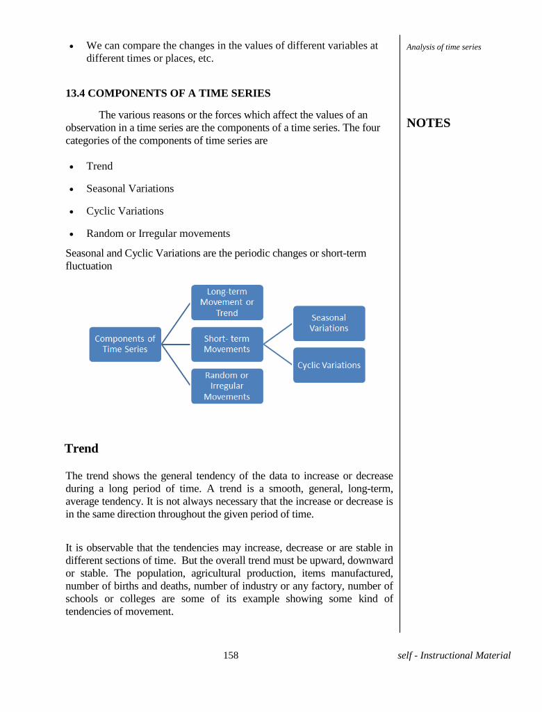
158 self - Instructional Material
We can compare the changes in the values of different variables at
different times or places, etc.
13.4 COMPONENTS OF A TIME SERIES
The various reasons or the forces which affect the values of an
observation in a time series are the components of a time series. The four
categories of the components of time series are
Trend
Seasonal Variations
Cyclic Variations
Random or Irregular movements
Seasonal and Cyclic Variations are the periodic changes or short-term
fluctuation
Trend
The trend shows the general tendency of the data to increase or decrease
during a long period of time. A trend is a smooth, general, long-term,
average tendency. It is not always necessary that the increase or decrease is
in the same direction throughout the given period of time.
It is observable that the tendencies may increase, decrease or are stable in
different sections of time. But the overall trend must be upward, downward
or stable. The population, agricultural production, items manufactured,
number of births and deaths, number of industry or any factory, number of
schools or colleges are some of its example showing some kind of
tendencies of movement.
Analysis of time series
NOTES
159 self - Instructional Material
Linear and Non-Linear Trend
If we plot the time series values on a graph in accordance with time t. The
pattern of the data clustering shows the type of trend. If the set of data
cluster more or less round a straight line, then the trend is linear otherwise it
is non-linear (Curvilinear).
Periodic Fluctuations
There are some components in a time series which tend to repeat
themselves over a certain period of time. They act in a regular spasmodic
manner.
Seasonal Variations
These are the rhythmic forces which operate in a regular and periodic
manner over a span of less than a year. They have the same or almost the
same pattern during a period of 12 months. This variation will be present in
a time series if the data are recorded hourly, daily, weekly, quarterly, or
monthly.
These variations come into play either because of the natural forces or man-
made conventions. The various seasons or climatic conditions play an
important role in seasonal variations. Such as production of crops depends
on seasons, the sale of umbrella and raincoats in the rainy season, and the
sale of electric fans and A.C. shoots up in summer seasons.
The effect of man-made conventions such as some festivals, customs,
habits, fashions, and some occasions like marriage is easily noticeable.
They recur themselves year after year. An upswing in a season should not
be taken as an indicator of better business conditions.
Cyclic Variations
The variations in a time series which operate themselves over a span of
more than one year are the cyclic variations. This oscillatory movement has
a period of oscillation of more than a year. One complete period is a cycle.
Th s cyc c m veme s s me mes c ed he ‘Bus ess Cyc e’.
It is a four-phase cycle comprising of the phases of prosperity, recession,
depression, and recovery. The cyclic variation may be regular are not
periodic. The upswings and the downswings in business depend upon the
joint nature of the economic forces and the interaction between them.
Random or Irregular Movements
There is another factor which causes the variation in the variable under
study. They are not regular variations and are purely random or irregular.
These fluctuations are unforeseen, uncontrollable, unpredictable, and are
erratic. These forces are earthquakes, wars, flood, famines, and any other
disasters.
Analysis of time series
NOTES
160 self - Instructional Material
UNIT-XIV MEASUREMENTS OF
TRENDS
14-1 MEASUREMENT OF TRENDS:
Secular trend is a long term movement in a time series. This
component represents basic tendency of the series. The following
methods are generally used to determine trend in any given time series.
The following methods are generally used to determine trend in any
given time series.
Graphic method or eye inspection method
Semi average method
Method of moving average
Method of least squares
Graphic method or eye inspection method
Graphic method is the simplest of all methods and easy to
understand. The method is as follows. First plot the given time series data
on a graph. Then a smooth free hand curve is drawn through the plotted
points in such a way that it represents general tendency of the series. As
the curve is drawn through eye inspection, this is also called as eye-
inspection method. The graphic method removes the short term
variations to show the basic tendency of the data. The trend line drawn
through the graphic method can be extended further to predict or estimate
values for the future time periods. As the method is subjective the
prediction may not be reliable.
Advantages
It is very simplest method for study trend values and easy to draw
trend.
Sometimes the trend line drawn by the statistician experienced in
computing trend may be considered better than a trend line fitted by
the use of a mathematical formula.
Although the free hand curves method is not recommended for
beginners, it has considerable merits in the hands of experienced
statisticians and widely used in applied situations.
Disadvantages:
This method is highly subjective and curve varies from person to
person who draws it.
Measurements of Trends
NOTES
161 self - Instructional Material
The work must be handled by skilled and experienced people.
Since the method is subjective, the prediction may not be reliable.
While drawing a trend line through this method a careful job has
to be done.
Method of Semi Averages:
In this method the whole data is divided in two equal parts with
respect to time. For example if we are given data from 1999 to 2016 i.e.
over a period of 18 years the two equal parts will be first nine years i.e.
from 1999 to 2007 and 2008 to 2016. In case of odd number of years like
9, 13, 17 etc. two equal parts can be made simply by omitting the middle
year. For example if the data are given for 19 years from 1998 to 2016
the two equal parts would be from 1998 to 2006 and from 2008 to 2016,
the middle year 2007 will be omitted. After the data have been divided
into two parts, an average (arithmetic mean) of each part is obtained. We
thus get two points. Each point is plotted against the mid year of the each
part. Then these two points are joined by a straight line which gives us
the trend line. The line can be extended downwards or upwards to get
intermediate values or to predict future values.
Advantages:
This method is simple to understand as compare to moving
average methodand method of least squares.
This is an objective method of measuring trend as everyone who
applies this method is bound to get the same result.
Disadvantages:
The method assumes straight line relationship between the plotted
points regardless of the fact whether that relationship exists or not.
The main drawback of this method is if we add some more data to
the original data then whole calculation is to be done again for the new
data to get the trend values and the trend line also changes.
As the Arithmetic Mean of each half is calculated, an extreme
value in any half will greatly affect the points and hence trend calculated
through these points may not be precise enough for forecasting the
future.
Method of Moving Average:
It is a method for computing trend values in a time series which
eliminates the short term and random fluctuations from the time series by
means of moving average. Moving average of a period m is a series of
successive arithmetic means of m terms at a time starting with 1st, 2nd ,
Measurements of Trends
NOTES
162 self - Instructional Material
3rd and so on. The first average is the mean of first m terms; the second
average is the mean of 2nd term to (m+1)th term and 3rd average is the
mean of 3rd term to (m+2)th term and so on.
If m is odd then the moving average is placed against the mid
value of the time interval it covers. But if m is even then the moving
average lies between the two middle periods which does not correspond
to any time period. So further steps has to be taken to place the moving
average to a particular period of time. For that we take 2-yearly moving
average of the moving averages which correspond to a particular time
period. The resultant moving averages are the trend values.
Advantages:
This method is simple to understand and easy to execute.
It has the flexibility in application in the sense that if we add
data for a few more time periods to the original data, the previous
calculations are not affected and we get a few more trend values.
It gives a correct picture of the long term trend if the trend is
linear.
If the period of moving average coincides with the period of
oscillation (cycle), the periodic fluctuations are eliminated.
The moving average has the advantage that it follows the general
movements of the data and that its shape is determined by the data rather
h he s s c ‟s ch ce f m hem c fu c .
Disadvantages:
For a moving average of 2m+1, one does not get trend values for
first m and last m periods.
As the trend path does not correspond to any mathematical;
function, it cannot be used for forecasting or predicting values for future
periods.
If the trend is not linear, the trend values calculated through
moving averages may not show the true tendency of data.
The choice of the period is sometimes left to the human judgment
and hence may carry the effect of human bias.
Method of Least Squares:
This method is most widely used in practice. It is mathematical
method and with its help a trend line is fitted to the data in such a manner
that the following two conditions are satisfied.
Measurements of Trends
NOTES
163 self - Instructional Material
(Y - Yc ) =0 i.e. the sum of the deviations of the actual values
of Y and the computed values of Y is zero.
(Y - Yc)2 is least, i.e. the sum of the squares of the deviations
of the actual values and the computed values is least.
The e b ed by h s me h d s c ed s he “ e f bes f ”.
This method of least squares may be used either to fit a straight line trend
or a parabolic trend.
Measurement of seasonal variations:
There is a simple method for measuring the seasonal variation
which involves simple averages.
Simple average method.
Step1. All the data are arranged by years and months( or quarters)
Step 2. Compute the simple averages ( arithmetic mean) for ith
month.
Step 3. Obtain the overall average of these averages and
=
Step 4. Seasonal indices for different months are calculated by
expressing monthly average as the percentage of the overall average
Thus seasonal index for ith
month =
Solved problems.
problem 1. use the method of least and fit a straight line trend to the
following data given from 82 to 92 . Hence estimate the trends value for
1993.
Year 82 83 84 85 86 87 88 89 90 91 92
Production
in quintals
45 46 44 47 42 41 39 42 45 40 48
Solution. Let the line of best fit be y = ax + b
Take X = x - 1987 and Y = y - 42
Then the line of best fit become Y = aX + b
The normal equations are = a + b
= a + nb when n = 11
Measurements of Trends
NOTES
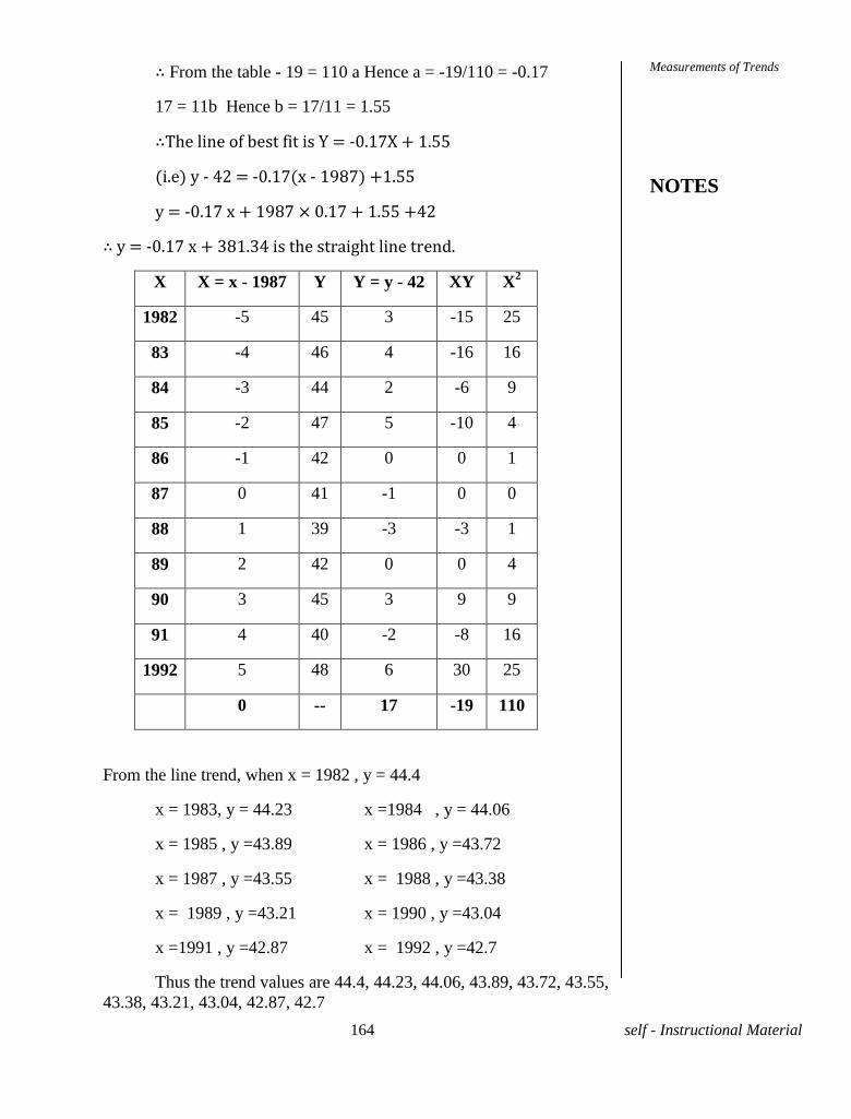
164 self - Instructional Material
∴ From the table - 19 = 110 a Hence a = -19/110 = -0.17
17 = 11b Hence b = 17/11 = 1.55
∴ f best fit is Y = -0.17X + 1.55
(i.e) y - 42 = -0.17(x - 1987) +1.55
y = -0.17 x + 1987 0.17 + 1.55 +42
∴ -0.17 x + 381.34 is the straight line trend.
X X = x - 1987 Y Y = y - 42 XY X2
1982 -5 45 3 -15 25
83 -4 46 4 -16 16
84 -3 44 2 -6 9
85 -2 47 5 -10 4
86 -1 42 0 0 1
87 0 41 -1 0 0
88 1 39 -3 -3 1
89 2 42 0 0 4
90 3 45 3 9 9
91 4 40 -2 -8 16
1992 5 48 6 30 25
0 -- 17 -19 110
From the line trend, when x = 1982 , y = 44.4
x = 1983, y = 44.23 x =1984 , y = 44.06
x = 1985 , y =43.89 x = 1986 , y =43.72
x = 1987 , y =43.55 x = 1988 , y =43.38
x = 1989 , y =43.21 x = 1990 , y =43.04
x =1991 , y =42.87 x = 1992 , y =42.7
Thus the trend values are 44.4, 44.23, 44.06, 43.89, 43.72, 43.55,
43.38, 43.21, 43.04, 42.87, 42.7
Measurements of Trends
NOTES
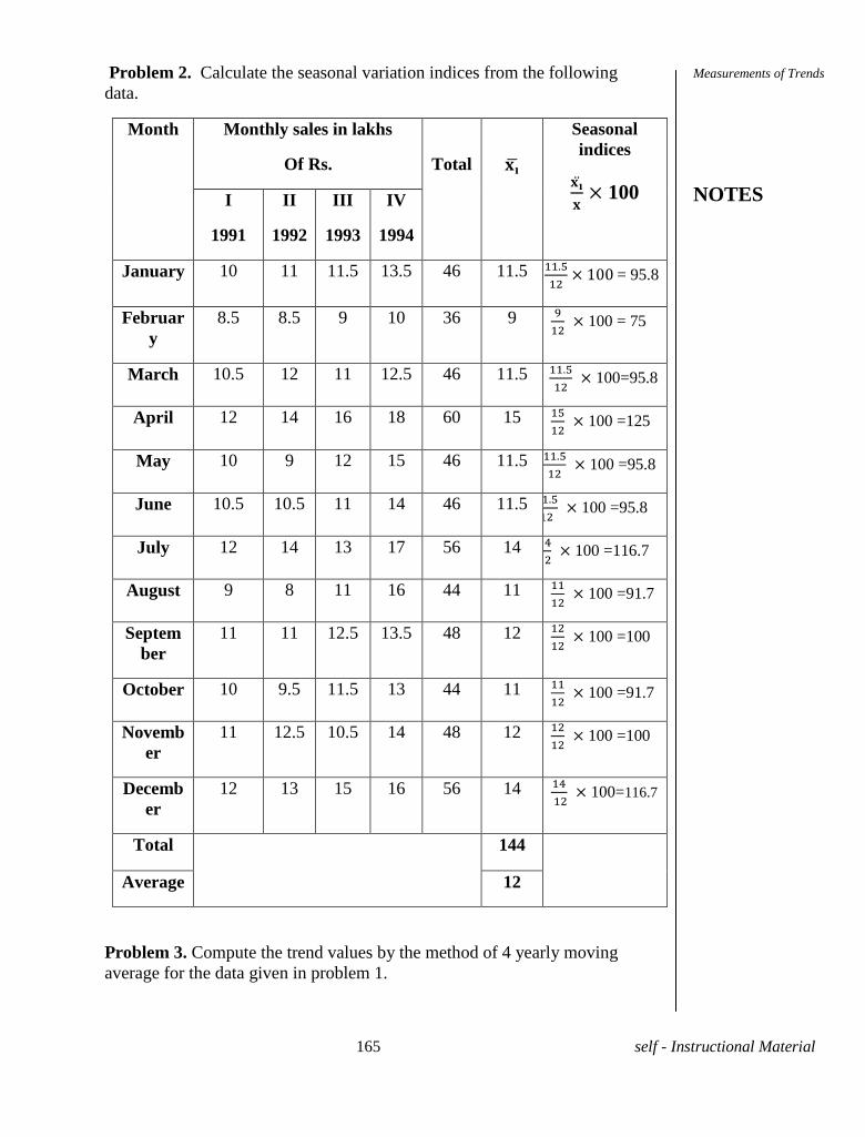
165 self - Instructional Material
Problem 2. Calculate the seasonal variation indices from the following
data.
Month Monthly sales in lakhs
Of Rs.
Total
Seasonal
indices
100 I
1991
II
1992
III
1993
IV
1994
January 10 11 11.5 13.5 46 11.5
= 95.8
Februar
y
8.5 8.5 9 10 36 9
100 = 75
March 10.5 12 11 12.5 46 11.5
100=95.8
April 12 14 16 18 60 15
100 =125
May 10 9 12 15 46 11.5
100 =95.8
June 10.5 10.5 11 14 46 11.5
100 =95.8
July 12 14 13 17 56 14
100 =116.7
August 9 8 11 16 44 11
100 =91.7
Septem
ber
11 11 12.5 13.5 48 12
100 =100
October 10 9.5 11.5 13 44 11
100 =91.7
Novemb
er
11 12.5 10.5 14 48 12
100 =100
Decemb
er
12 13 15 16 56 14
100=116.7
Total 144
Average 12
Problem 3. Compute the trend values by the method of 4 yearly moving
average for the data given in problem 1.
Measurements of Trends
NOTES
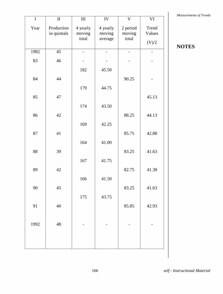
166 self - Instructional Material
I
Year
II
Production
in quintals
III
4 yearly
moving
total
IV
4 yearly
moving
average
V
2 period
moving
total
VI
Trend
Values
(V)/2
1982
83
84
85
86
87
88
89
90
91
1992
45
46
44
47
42
41
39
42
45
40
48
-
-
182
179
174
169
164
167
166
175
-
-
-
45.50
44.75
43.50
42.25
41.00
41.75
41.50
43.75
-
-
-
90.25
88.25
85.75
83.25
82.75
83.25
85.85
-
-
-
-
45.13
44.13
42.88
41.63
41.38
41.63
42.93
-
Measurements of Trends
NOTES
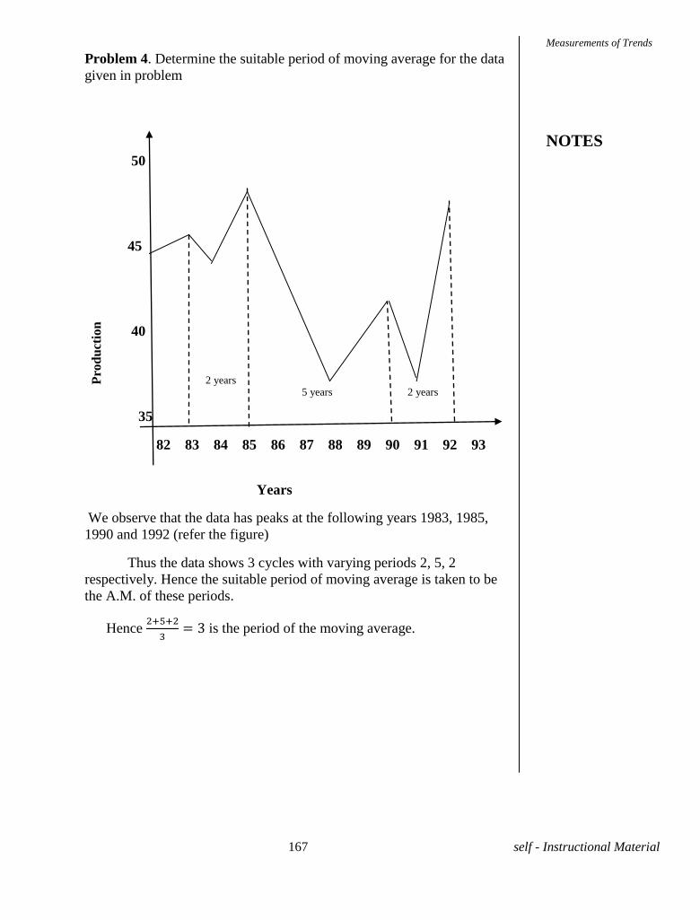
167 self - Instructional Material
Problem 4. Determine the suitable period of moving average for the data
given in problem
50
45
40
35
82 83 84 85 86 87 88 89 90 91 92 93
Years
We observe that the data has peaks at the following years 1983, 1985,
1990 and 1992 (refer the figure)
Thus the data shows 3 cycles with varying periods 2, 5, 2
respectively. Hence the suitable period of moving average is taken to be
the A.M. of these periods.
Hence
is the period of the moving average.
2 years 5 years 2 years
Pro
du
ctio
n
Measurements of Trends
NOTES
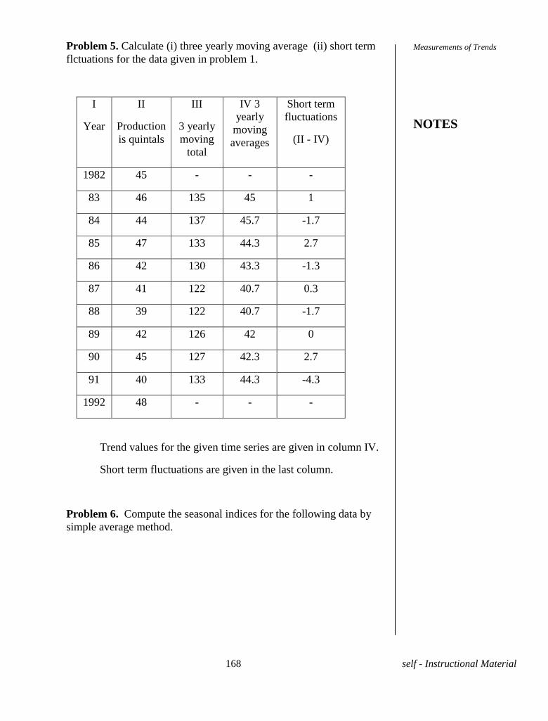
168 self - Instructional Material
Problem 5. Calculate (i) three yearly moving average (ii) short term
flctuations for the data given in problem 1.
I
Year
II
Production
is quintals
III
3 yearly
moving
total
IV 3
yearly
moving
averages
Short term
fluctuations
(II - IV)
1982 45 - - -
83 46 135 45 1
84 44 137 45.7 -1.7
85 47 133 44.3 2.7
86 42 130 43.3 -1.3
87 41 122 40.7 0.3
88 39 122 40.7 -1.7
89 42 126 42 0
90 45 127 42.3 2.7
91 40 133 44.3 -4.3
1992 48 - - -
Trend values for the given time series are given in column IV.
Short term fluctuations are given in the last column.
Problem 6. Compute the seasonal indices for the following data by
simple average method.
Measurements of Trends
NOTES
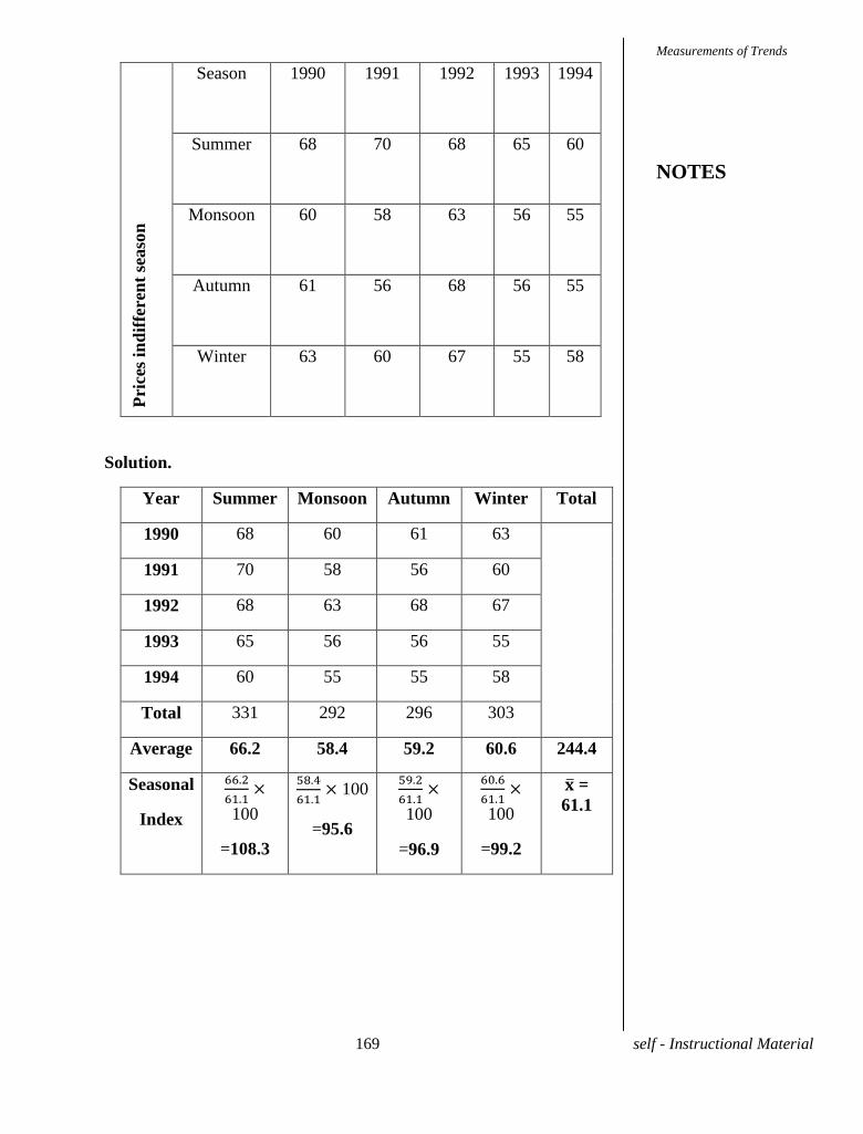
169 self - Instructional Material
Pri
ces
ind
iffe
ren
t se
aso
n
Season 1990 1991 1992 1993 1994
Summer 68 70 68 65 60
Monsoon 60 58 63 56 55
Autumn 61 56 68 56 55
Winter 63 60 67 55 58
Solution.
Year Summer Monsoon Autumn Winter Total
1990 68 60 61 63
1991 70 58 56 60
1992 68 63 68 67
1993 65 56 56 55
1994 60 55 55 58
Total 331 292 296 303
Average 66.2 58.4 59.2 60.6 244.4
Seasonal
Index
100
=108.3
100
=95.6
100
=96.9
100
=99.2
=
61.1
Measurements of Trends
NOTES
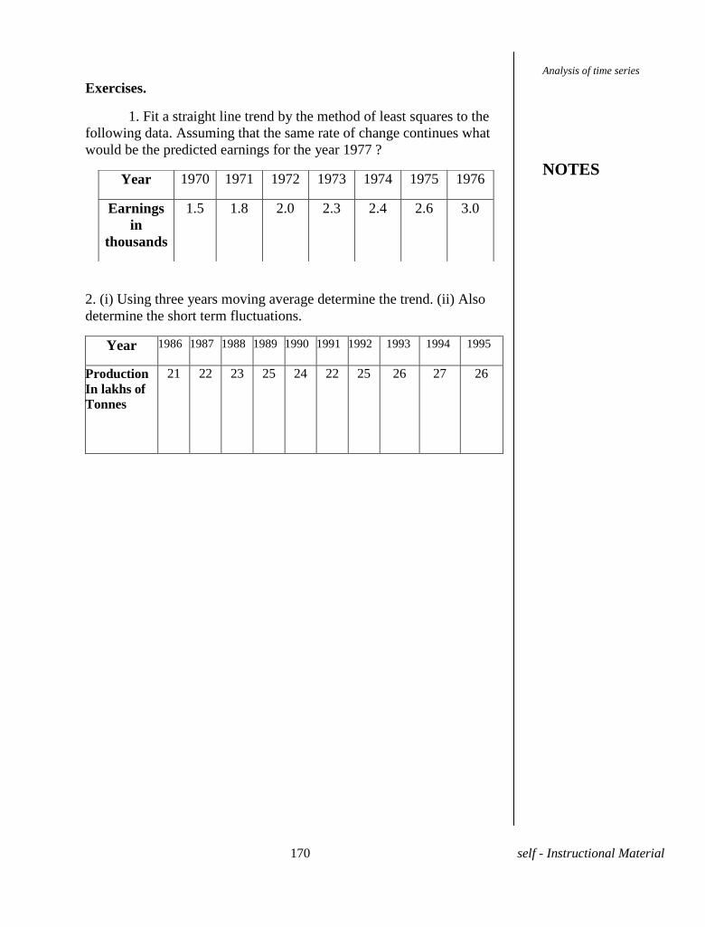
170 self - Instructional Material
Exercises.
1. Fit a straight line trend by the method of least squares to the
following data. Assuming that the same rate of change continues what
would be the predicted earnings for the year 1977 ?
2. (i) Using three years moving average determine the trend. (ii) Also
determine the short term fluctuations.
Year 1986 1987 1988 1989 1990 1991 1992 1993 1994 1995
Production
In lakhs of
Tonnes
21 22 23 25 24 22 25 26 27 26
Year 1970 1971 1972 1973 1974 1975 1976
Earnings
in
thousands
1.5 1.8 2.0 2.3 2.4 2.6 3.0
Analysis of time series
NOTES
171 self - Instructional Material
DISTANCE EDUCATION – CBCS-(2018-19 Academic Year Onwards).
Question Paper Pattern(ESE)- Theory
(UG/PG/P.G Diploma Programmes)
Time : 3 hours Maximum :75 Marks
Part – A (10 X 2= 20 Marks)
Answer all questions
1.
2.
3.
4.
5.
6.
7.
8.
9.
10.
Part –B (5 X 5= 25 Marks)
Answer all questions choosing either (a) or (b)
11.a.
(or)
b.
12.a.
(or)
b.
13.a.
(or)
b.
14.a.
(or)
b.
15.a.
(or)
b.
Part –C (3 X 10 = 30 Marks)
(Answer any 3 out of 5 questions)
16.
17.
18.
19.
20.