Embed Size (px)
Citation preview
Ruprecht-Karls-Universitat HeidelbergFakultat fur Mathematik und Informatik
Statistical Postprocessing ofEnsemble Forecasts for Temperature:The Importance of Spatial Modeling
Diplomarbeit vonKira Feldmann
Juni 2012
Betreuer: Dr. Michael ScheuererDr. Thordis ThorarinsdottirProf. Dr. Tilmann Gneiting

Abstract
In the recent past, ensemble prediction systems have become state of the art in themeteorological community. However, ensembles often underestimate the uncertainty innumerical weather prediction, resulting in underdispersive and thus uncalibrated forecasts.In order to employ the full potential of the ensemble, statistical postprocessing is needed.However, many of the current approaches, such as Bayesian model averaging (BMA) orensemble model output statistics (EMOS), focus on forecasts at single locations, not takingspatial correlation between different observation sites into account. In this thesis, wediscuss the existing method of spatial BMA, which combines the geostatistical outputperturbation method (GOP) for modeling the spatial structure of the observation field,with BMA, in order to produce calibrated and sharp forecasts for whole weather fields.We propose a similar approach that employs EMOS instead of BMA. In a case study, weapply the methods to 21-hour ahead forecasts of surface temperature over Germany, issuedby COSMO-DE-EPS. The multivariate forecasts were capable of capturing the spatialstructure of the weather field and turn out to be calibrated and sharp, while showing animprovement over the raw ensemble as well as the reference forecasts.
Zusammenfassung
In der nahen Vergangenheit sind ensemblebasierte Wettervorhersagesysteme immer populä-rer geworden. Dennoch unterschätzen die Ensembles häufig die Unsicherheit numerischerWettervorhersagen, wodurch die Vorhersagen unterdispersiv werden und folglich nicht kali-briert sind. Um die volle Leistungsfähigkeit des Ensembles zu entfalten, werden statistischeNachbearbeitungsverfahren benötigt. Jedoch konzentriert sich die Mehrheit dieser Metho-den, wie unter anderem Bayesian model averaging (BMA) oder ensemble model outputstatistics (EMOS), auf Vorhersagen an einzelnen Orten und berücksichtigt dabei nicht dieräumliche Korrelation zwischen den verschiedenen Beobachtungsstationen. In dieser Arbeitdiskutieren wir die vorhandene Methode spatial BMA, welche die Kombination von zweiNachbearbeitungsverfahren darstellt. Geostatistcal output perturbation method (GOP)modelliert die räumliche Struktur des Wetterfeldes und BMA inkludiert die Ensembleinfor-mation, so dass kalibrierte und scharfe Wettervorhersagen für ganze Wetterfelder produziertwerden. Wir schlagen zusätzlich einen ähnlichen Ansatz vor, der BMA durch EMOS ersetzt.In einer Fallstudie wenden wir die Methoden auf 21-stündige Temperaturvorhersagen vonCOSMO-DE-EPS für Deutschland an. Die multivariaten Vorhersagen schaffen es, die räum-liche Struktur des Wetterfeldes wiederzugeben und erzeugen somit scharfe und kalibrierteVorhersagen, die eine Verbesserung gegenüber dem unbearbeiteten Ensemble sowie denReferenzvorhersagemethoden darstellen.
3


Contents
1 Introduction 7
2 COSMO-DE-EPS 112.1 Properties and Construction . . . . . . . . . . . . . . . . . . . . . . . . . . 112.2 Forecasting Performance . . . . . . . . . . . . . . . . . . . . . . . . . . . . 12
3 Univariate Postprocessing 173.1 Bayesian Model Averaging (BMA) . . . . . . . . . . . . . . . . . . . . . . . 173.2 Ensemble Model Output Statistics (EMOS) . . . . . . . . . . . . . . . . . 193.3 Linear Model Forecast (LMF) . . . . . . . . . . . . . . . . . . . . . . . . . 203.4 Reference Forecasts . . . . . . . . . . . . . . . . . . . . . . . . . . . . . . . 213.5 Results . . . . . . . . . . . . . . . . . . . . . . . . . . . . . . . . . . . . . . 223.6 Extension: EMOS with Student’s t-distribution . . . . . . . . . . . . . . . 23
4 Spatial Postprocessing 294.1 Geostatistical Output Perturbation (GOP) . . . . . . . . . . . . . . . . . . 294.2 Spatial BMA . . . . . . . . . . . . . . . . . . . . . . . . . . . . . . . . . . 334.3 Spatial EMOS+ . . . . . . . . . . . . . . . . . . . . . . . . . . . . . . . . . 344.4 Reference Forecasts . . . . . . . . . . . . . . . . . . . . . . . . . . . . . . . 364.5 Results . . . . . . . . . . . . . . . . . . . . . . . . . . . . . . . . . . . . . . 37
4.5.1 Different Modeling of Spatial Structure for GOP . . . . . . . . . . . 374.5.2 Overall Performance of the Models . . . . . . . . . . . . . . . . . . 38
5 Discussion 47
5

CONTENTS
A Verification Methods 51A.1 Assessing Calibration . . . . . . . . . . . . . . . . . . . . . . . . . . . . . . 52A.2 Assessing Sharpness . . . . . . . . . . . . . . . . . . . . . . . . . . . . . . . 54A.3 Proper Scoring Rules . . . . . . . . . . . . . . . . . . . . . . . . . . . . . . 54A.4 Empirical Variogram Coverage . . . . . . . . . . . . . . . . . . . . . . . . . 57
B Plots of the Empirical Variograms 58
C Further Verification Results 60
6

Chapter 1
Introduction
”My interest is in the future because I am going to spend the rest of my life there.”C.F. Kettering (1876-1958), inventor, scientist, engineer, businessman, philosopher
Predictions of the future have always been of great interest for mankind. Especiallytoday, weather forecasts are a matter of high economical and social value, as they findapplications in many different areas. Accurate predictions are essential for the growing fieldof renewable energies, management of air traffic, and natural disaster control, just to namea few.
In the past century, huge developments have been made in the field of forecastingweather quantities. With the advent of computer simulation, the rise of deterministicnumerical weather prediction began in the early 1950s. At the same time, concerns overrigorous determinism, based on the principle that the future state of a system can beentirely described by its present state, started to grow (Lewis, 2005). Following the path ofdeterminism, sources of uncertainty in numerical weather forecasts, such as imperfectionsin model formulation or insufficiency in the description of initial and boundary conditions,are not addressed (Leutbecher and Palmer, 2008).
In order to resolve these shortcomings, the first ensemble prediction systems weredeveloped in the early 1990s (Lewis, 2005). An ensemble consists of multiple runs of thenumerical weather prediction model, with variations in mathematical representations of thedevelopment of the atmosphere, initial conditions or lateral boundaries, and thus seeks toquantify the sources of uncertainty in deterministic forecasts. However, ensemble predictionsystems are often underdispersed and tend to be biased (Hamill and Colucci, 1997).
7
CHAPTER 1. Introduction
To address these issues, a variety of statistical postprocessing methods for ensembleshave been proposed (Wilks and Hamill, 2007). These models yield probabilistic forecasts,meaning that they deliver a predictive probability distribution for the weather variable ofinterest, which generally outperforms the raw ensemble in terms of satisfying the underlyinggoal of “maximizing sharpness subject to calibration” (Gneiting et al., 2007).
However, the majority of these methods is only applicable to univariate weather quan-tities at a single location and does not model spatial dependencies between differentobservation sites, which are of great importance when considering composite quantities,such as minima, maxima, totals or averages. These aggregated quantities are crucial e.g. forhighway maintenance operations or flood management. Based on well-established univariatepostprocessing techniques, probabilistic forecasts of any composite quantity of interestare straightforward to calculate. However, there is a high possibility that the predictiveuncertainty is estimated poorly, as the model does not capture that the site-specific pre-dictive uncertainties are correlated which has a great impact on the overall uncertainty(Thorarinsdottir et al., 2012).
In the case of deterministic temperature forecasts, Gel et al. (2004) propose the geo-statistical output perturbation (GOP) method, that uses a geostatistical model in orderto simulate spatially consistent temperature forecasts fields. In this thesis, we discuss theapproach by Berrocal et al. (2007), that combines the univariate postprocessing methodBaysian model averaging (BMA) with GOP. Based on ensemble prediction systems, BMAyields predictive probability density functions, which are weighted averages of densitiescentered at the bias-corrected forecasts of the individual ensemble members (Raftery et al.,2005). By uniting BMA and GOP, calibrated probabilistic forecasts of entire weather fieldsare produced based on ensemble prediction systems. In a similar way, we propose combiningthe univariate postprocessing method based on ensemble model output statistics (EMOS),which produces normal predictive density functions for temperature (Gneiting et al., 2005),with GOP in order to obtain the same goal.
The remainder of this thesis is organized as follows. Chapter 2 gives an introduction toCOSMO-DE-EPS, the 20-member ensemble prediction system developed by the GermanMeteorological Service (DWD). We describe its construction and evaluate the predictiveperformance of 21-hour ahead forecasts of surface temperature over Germany in 2011.In Chapter 3, we provide details of the univariate postprocessing methods EMOS andBMA as well as a rather simple approach, based solely on least squares regression. Ina case study, we apply these models to COSMO-DE-EPS and compare their predictiveperformance with reference forecasts. At the end of this chapter, we investigate an EMOS
8

CHAPTER 1. Introduction
approach, where we replace the commonly used normal distribution with a Student’st-distribution, in order to cope with some of the challenges in statistical postprocessingof COSMO-DE-EPS. Chapter 4 describes the multivariate GOP and different ways ofestimating the corresponding parameters. Then, we combine GOP with EMOS+ and BMArespectively in order to produce calibrated and sharp forecasts for entire weather fields,followed by a case study based on COSMO-DE-EPS. The thesis closes with a discussion inChapter 5, where we summarize the results, describe possible improvements of the methods,address some unresolved issues and hint at subjects of further research. The Appendixdescribes verification methods, compares the empirical variogram calculation of two differentR packages and provides additional results for the models presented in Chapter 4.
9


Chapter 2
COSMO-DE-EPS
This chapter serves as an introduction to the ensemble forecasting system COSMO-DE-EPS(COnsortium for Small-scale MOdeling - DE - Ensemble Prediction System), which we willuse as a basis for the competing postprocessing methods in the following chapters. Startingwith some properties of the ensemble, we then describe its construction and end with anevaluation of the forecasting performance.
2.1 Properties and Construction
COSMO-DE-EPS is a 20-member ensemble prediction system, developed by the GermanMeteorological Service, with a planned extension to 40 members. Its pre-operational phasestarted on 9 December 2010 and the operational phase was launched on 22 May 2012 (Theisand Gebhardt, 2012). The forecasts are made for lead times from 0 up to 21 hours on agrid covering Germany. The horizontal and vertical spacing between grid-points is 2.8 km,resulting in meso-γ-scale predictions (Peralta and Buchhold, 2011; Theis et al., 2011).
The EPS is based on a convection-permitting configuration, COSMO-DE, of the numeri-cal weather prediction model COSMO (Steppeler et al., 2003; Baldauf et al., 2011). Usually,prediction ensembles are created by perturbing the initial conditions and model physics ofthe corresponding numerical forecast model, based on an idea by Leith (1974). In case ofthe COSMO-DE-EPS, variations in lateral boundary conditions are also included, in orderto generate multiple deterministic predictions for one location (Gebhardt et al., 2011). Inparticular, five different configurations of the COSMO-DE model yield perturbations in themodel physics. On the other hand, the ensemble member forecasts rely on diverse lateral
11
CHAPTER 2. COSMO-DE-EPS
IFS
GME
GFS
GSM
1 2 3 4 5
E1 E2 E3 E4 E5
E6 E7 E8 E9 E10
E11 E12 E13 E14 E15
E16 E17 E18 E19 E20
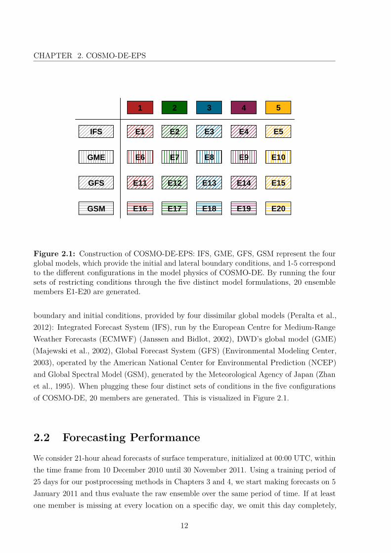
Figure 2.1: Construction of COSMO-DE-EPS: IFS, GME, GFS, GSM represent the fourglobal models, which provide the initial and lateral boundary conditions, and 1-5 correspondto the different configurations in the model physics of COSMO-DE. By running the foursets of restricting conditions through the five distinct model formulations, 20 ensemblemembers E1-E20 are generated.
boundary and initial conditions, provided by four dissimilar global models (Peralta et al.,2012): Integrated Forecast System (IFS), run by the European Centre for Medium-RangeWeather Forecasts (ECMWF) (Janssen and Bidlot, 2002), DWD’s global model (GME)(Majewski et al., 2002), Global Forecast System (GFS) (Environmental Modeling Center,2003), operated by the American National Center for Environmental Prediction (NCEP)and Global Spectral Model (GSM), generated by the Meteorological Agency of Japan (Zhanet al., 1995). When plugging these four distinct sets of conditions in the five configurationsof COSMO-DE, 20 members are generated. This is visualized in Figure 2.1.
2.2 Forecasting Performance
We consider 21-hour ahead forecasts of surface temperature, initialized at 00:00 UTC, withinthe time frame from 10 December 2010 until 30 November 2011. Using a training period of25 days for our postprocessing methods in Chapters 3 and 4, we start making forecasts on 5January 2011 and thus evaluate the raw ensemble over the same period of time. If at leastone member is missing at every location on a specific day, we omit this day completely,
12
CHAPTER 2. COSMO-DE-EPS
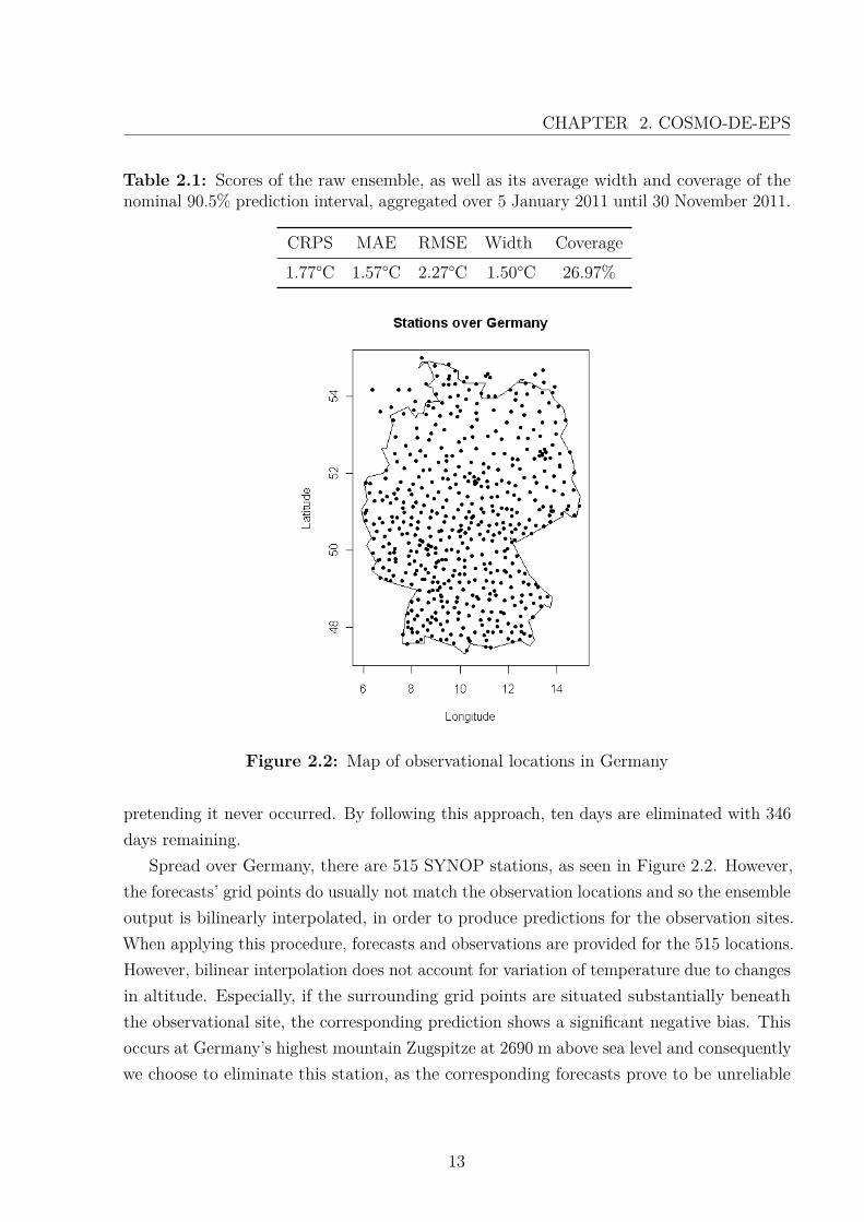
Table 2.1: Scores of the raw ensemble, as well as its average width and coverage of thenominal 90.5% prediction interval, aggregated over 5 January 2011 until 30 November 2011.
CRPS MAE RMSE Width Coverage1.77°C 1.57°C 2.27°C 1.50°C 26.97%
Figure 2.2: Map of observational locations in Germany
pretending it never occurred. By following this approach, ten days are eliminated with 346days remaining.
Spread over Germany, there are 515 SYNOP stations, as seen in Figure 2.2. However,the forecasts’ grid points do usually not match the observation locations and so the ensembleoutput is bilinearly interpolated, in order to produce predictions for the observation sites.When applying this procedure, forecasts and observations are provided for the 515 locations.However, bilinear interpolation does not account for variation of temperature due to changesin altitude. Especially, if the surrounding grid points are situated substantially beneaththe observational site, the corresponding prediction shows a significant negative bias. Thisoccurs at Germany’s highest mountain Zugspitze at 2690 m above sea level and consequentlywe choose to eliminate this station, as the corresponding forecasts prove to be unreliable
13
CHAPTER 2. COSMO-DE-EPS
Rank Histogram
Rank
Rel
ativ
e F
requ
ency
0.0
0.2
0.4
0.6
1 5 9 13 17 21
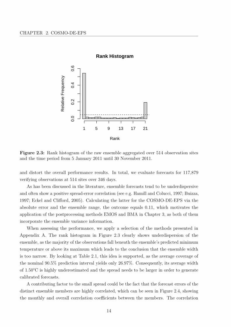
Figure 2.3: Rank histogram of the raw ensemble aggregated over 514 observation sitesand the time period from 5 January 2011 until 30 November 2011.
and distort the overall performance results. In total, we evaluate forecasts for 117,879verifying observations at 514 sites over 346 days.
As has been discussed in the literature, ensemble forecasts tend to be underdispersiveand often show a positive spread-error correlation (see e.g. Hamill and Colucci, 1997; Buizza,1997; Eckel and Clifford, 2005). Calculating the latter for the COSMO-DE-EPS via theabsolute error and the ensemble range, the outcome equals 0.11, which motivates theapplication of the postprocessing methods EMOS and BMA in Chapter 3, as both of themincorporate the ensemble variance information.
When assessing the performance, we apply a selection of the methods presented inAppendix A. The rank histogram in Figure 2.3 clearly shows underdispersion of theensemble, as the majority of the observations fall beneath the ensemble’s predicted minimumtemperature or above its maximum which leads to the conclusion that the ensemble widthis too narrow. By looking at Table 2.1, this idea is supported, as the average coverage ofthe nominal 90.5% prediction interval yields only 26.97%. Consequently, its average widthof 1.50°C is highly underestimated and the spread needs to be larger in order to generatecalibrated forecasts.
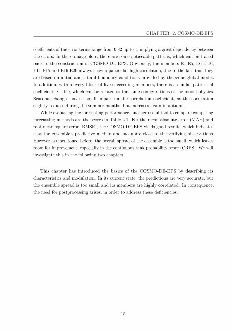
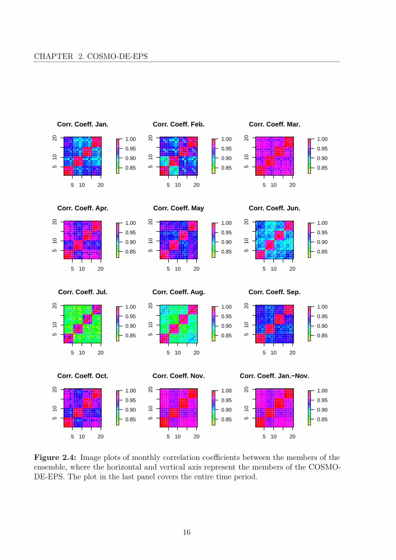
A contributing factor to the small spread could be the fact that the forecast errors of thedistinct ensemble members are highly correlated, which can be seen in Figure 2.4, showingthe monthly and overall correlation coefficients between the members. The correlation
14
CHAPTER 2. COSMO-DE-EPS
coefficients of the error terms range from 0.82 up to 1, implying a great dependency betweenthe errors. In these image plots, there are some noticeable patterns, which can be tracedback to the construction of COSMO-DE-EPS. Obviously, the members E1-E5, E6-E-10,E11-E15 and E16-E20 always show a particular high correlation, due to the fact that theyare based on initial and lateral boundary conditions provided by the same global model.In addition, within every block of five succeeding members, there is a similar pattern ofcoefficients visible, which can be related to the same configurations of the model physics.Seasonal changes have a small impact on the correlation coefficient, as the correlationslightly reduces during the summer months, but increases again in autumn.
While evaluating the forecasting performance, another useful tool to compare competingforecasting methods are the scores in Table 2.1. For the mean absolute error (MAE) androot mean square error (RMSE), the COSMO-DE-EPS yields good results, which indicatesthat the ensemble’s predictive median and mean are close to the verifying observations.However, as mentioned before, the overall spread of the ensemble is too small, which leavesroom for improvement, especially in the continuous rank probability score (CRPS). We willinvestigate this in the following two chapters.
This chapter has introduced the basics of the COSMO-DE-EPS by describing itscharacteristics and modulation. In its current state, the predictions are very accurate, butthe ensemble spread is too small and its members are highly correlated. In consequence,the need for postprocessing arises, in order to address these deficiencies.
15
CHAPTER 2. COSMO-DE-EPS
5 10 20
510
20
Corr. Coeff. Jan.
0.85
0.90
0.95
1.00
5 10 20
510
20
Corr. Coeff. Feb.
0.85
0.90
0.95
1.00
5 10 20
510
20
Corr. Coeff. Mar.
0.85
0.90
0.95
1.00
5 10 20
510
20
Corr. Coeff. Apr.
0.85
0.90
0.95
1.00
5 10 20
510
20
Corr. Coeff. May
0.85
0.90
0.95
1.00
5 10 20
510
20
Corr. Coeff. Jun.
0.85
0.90
0.95
1.00
5 10 20
510
20
Corr. Coeff. Jul.
0.85
0.90
0.95
1.00
5 10 20
510
20
Corr. Coeff. Aug.
0.85
0.90
0.95
1.00
5 10 20
510
20
Corr. Coeff. Sep.
0.85
0.90
0.95
1.00
5 10 20
510
20
Corr. Coeff. Oct.
0.85
0.90
0.95
1.00
5 10 20
510
20
Corr. Coeff. Nov.
0.85
0.90
0.95
1.00
5 10 20
510
20
Corr. Coeff. Jan.−Nov.
0.85
0.90
0.95
1.00
Figure 2.4: Image plots of monthly correlation coefficients between the members of theensemble, where the horizontal and vertical axis represent the members of the COSMO-DE-EPS. The plot in the last panel covers the entire time period.
16
Chapter 3
Univariate Postprocessing
Most forecast ensembles, including the COSMO-DE-EPS (introduced in Chapter 2), showa positive spread-error correlation, while at the same time being uncalibrated. In order toaddress theses issues, a variety of statistical postprocessing techniques have been developed.In this chapter, we present different methods for univariate postprocessing of ensembleforecasts. All the procedures have in common that they yield full predictive probabilitydistributions, which strive to satisfy the underlying goal of “maximizing sharpness subjectto calibration” (Gneiting et al., 2007). In this thesis, we focus on techniques for thepostprocessing of temperature.
At first, we briefly demonstrate the principles of the well known techniques BMAand EMOS, followed by a method which is solely based on least squares regression. Wename this method linear model forecasts (LMF). Subsequently, we explain procedures toobtain reference forecasts in order to compare the overall predictive performance. Afterdiscussing the application of all techniques to the COSMO-DE-EPS, we finalize with anEMOS approach, where we replace the commonly used normal distribution with a Student’st-distribution, in an attempt to resolve some of the issues that arise in the statisticalpostprocessing of COSMO-DE-EPS.
3.1 Bayesian Model Averaging (BMA)
BMA is a standard statistical approach for combining competing statistical models and hasa broad application in e.g. social and health sciences (Hoeting et al., 1999). Its advantageover other techniques, such as conventional regression analysis, is based on the fact that
17
CHAPTER 3. Univariate Postprocessing
BMA makes use of multiple models, in contrast to methods which soley use a single modelthat is deemed to be the best. Only using a single model often leads to an underestimationof the uncertainty in the process of model selection. In this thesis, we follow the extension ofBMA from statistical models to dynamical models by Raftery et al. (2005), for the purposeof producing calibrated and sharp predictive distributions.
Let ys denote the weather variable of interest at location s ∈ S, and f1s, ..., fMs thecorresponding forecasts of the M -member ensemble. In the framework of BMA, we assigneach member a conditional probability density function pm (ys|fms), or kernel density, whichwe can interpret as the conditional density of ys, given member m ∈ M being the mostskillful within the ensemble. Then, the predictive density for ys equals
p (ys|f1s, ..., fMs) =M∑m=1
wmpm (ys|fms) ,
where w1, ..., wM are non-negative weights that add up to 1. The weights are determined bythe member’s skill in the training period; a higher weight reflects a more reliable member,whereas a lower weight is associated with a weak performance.
In the setting of BMA, temperature is modeled with a normal distribution. Thus, thekernels are univariate normal densities, centered at each member’s bias-corrected forecastams + bmsfms,
ys|fms ∼ N (ams + bmsfms, σ2)
with a common variance σ2.If it is necessary to produce deterministic forecasts, the BMA predictive mean, which is
a weighted average over the bias-corrected forecast,
E (y|f1, ..., fM) =M∑m=1
wm (am + bmfm)
can be useful. The overall variance of ys in the BMA setting is
Var(ys|f1s, .., fms) =M∑m=1
wm
((am + bmfms)−
M∑m=1
wm (am + bmfms))2
+ σ2,
where the first part of the sum on the right-hand side is the between-forecast variance whilethe second part represents the within-forecast variance.
18
CHAPTER 3. Univariate Postprocessing
Given a set of verifying observations yst and associated ensemble forecasts f1st, ..., fMst
for day t within a training period T , the BMA parameters are obtained in three steps. First,the member-specific parameters am and bm, for m = 1, ...,M , are individually determinedvia simple linear regression. In the second step, the weights wm, m = 1, ...,M , and thevariance σ2 are estimated by maximizing the log-likelihood function
l(w1, ..., wM , σ2) =∑s,t
log(
M∑m=1
wmp (yt|fkst)),
which, for simplicity, is based on the assumption that the forecast errors are independentin space and time. However, the maximum cannot be found analytically and Rafteryet al. (2005) thus employ the expectation–maximization (EM) algorithm. In the final andvoluntary step, the parameter estimate for σ2 may be refined by minimizing the CRPS, aproper scoring rule described in Appendix A, over the training period. When implementingthe BMA approach, we utilize the R package ensembleBMA by Fraley et al. (2011), whichyields the desired predictive distributions.
Apart from generating forecasts for normally distributed variables, such as temperatureor sea level pressure, BMA approaches for other weather quantities have been studied.Sloughter et al. (2007) propose a gamma distribution with a point mass in zero for modelingprecipitation, and Sloughter et al. (2010) present a BMA method to predict wind speedusing a gamma distribution. In addition, Bao et al. (2010) describe future wind directionsvia von Mises distributions.
3.2 Ensemble Model Output Statistics (EMOS)
EMOS, also called non-homogeneous Gaussian regression, is a form of multiple linearregression and an extension to the model output statistics technique. In contrast to BMA,EMOS is based on a single predictive density, whose parameters depend on the ensembleforecasts.
For temperature, a normal distribution is again employed to describe the future state ofthe variable (Gneiting et al., 2005). At location s ∈ S, the predictive distribution is
ys|f1s, ..., fMs ∼ N (a1 + b1f1s + ...+ bMfMs, c+ dS2s ),
19
CHAPTER 3. Univariate Postprocessing
which forms a linear model with the forecasts as predictors and the temperature ys aspredictand. The variance is modeled as a linear function of the ensemble variance S2
s .In this approach, the variance term counteracts the underdispersion of the ensemble,while additionally accounting for the positive spread-error correlation by incorporating theensemble information.
In contrast to BMA, the coefficients b1, ..., bM can take any value in R. However, negativevalues are difficult to interpret. Hence, the authors suggest restricting the coefficients to benon-negative and name this approach EMOS+. In this extended framework, the coefficientsreflect the relative performance of the ensemble members over the training period. Wefurther investigate a simpler variant, EMOS mean, where the ensemble mean is used as apredictor rather than the individual members.
For the calculation of the parameters, Gneiting et al. (2005) use minimum CRPS andmaximum likelihood estimation. According to their results, the minimum CRPS estimationoutperforms the latter and hence we employ this method as well. Over a set of trainingdata which contains the past forecasts and corresponding observations, the parametersoptimizing the score are chosen. In the case of a normal distribution, the CRPS can bewritten in a closed form (Gneiting et al., 2005) and the computational cost is thereforesubstantially reduced.
Further developments of EMOS for wind speed, wind gust and wind vectors can befound in Thorarinsdottir and Gneiting (2010), Thorarinsdottir and Johnson (2012) andSchuhen et al. (2012), respectively.
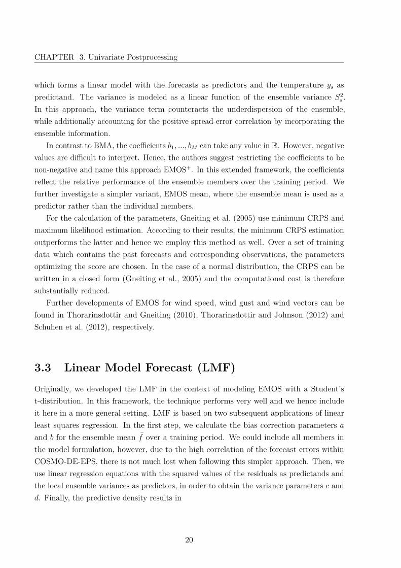
3.3 Linear Model Forecast (LMF)
Originally, we developed the LMF in the context of modeling EMOS with a Student’st-distribution. In this framework, the technique performs very well and we hence includeit here in a more general setting. LMF is based on two subsequent applications of linearleast squares regression. In the first step, we calculate the bias correction parameters aand b for the ensemble mean f over a training period. We could include all members inthe model formulation, however, due to the high correlation of the forecast errors withinCOSMO-DE-EPS, there is not much lost when following this simpler approach. Then, weuse linear regression equations with the squared values of the residuals as predictands andthe local ensemble variances as predictors, in order to obtain the variance parameters c andd. Finally, the predictive density results in
20

CHAPTER 3. Univariate Postprocessing
ys|f1s, ..., fMs ∼ N (a+ bf , c+ dS2),
where S represents the standard deviation of the ensemble.
3.4 Reference Forecasts
In order to compare the postprocessing methods discussed above with standard approaches,we also include some simpler techniques. Error dressing and the bias-corrected ensemble areboth based on ensemble predictions systems, whereas the climatology ensemble is generatedvia past observations.
Error Dressing
Error dressing, proposed by Gneiting et al. (2008), is an effortless way of postprocessingensemble outputs, which accounts for bias and dispersion errors. We employ a global variantof the method, where at each station s ∈ S we calculate the empirical errors es = ys − fs ofthe ensemble mean fs over the training period. Let e denote the mean of the sample ofempirical errors over all stations and σ2 the empirical variance, then the predictive densityequals
ys|f1s, ..., fMs ∼ N (fs + e, σ2).
Bias-Corrected Ensemble
The bias-corrected ensemble is a slight variation of the original ensemble, which oftenoutperforms the former. Considering each member individually, we use linear least squaresregression, with the forecasts fmst as predictors and the verifying observations yst aspredictands for day t in the training period T . When following this approach, we obtainthe member-specific bias-correcting parameters am,t+1, bm,t+1 for the succeeding day t+ 1.Then, the values am,t+1 + bm,t+1fm,s,t+1, m = 1, ...,M , form the bias-corrected ensemble.
Climatology
In contrast to the aforementioned methods, the climatology ensemble is not based on an EPS,instead past observations from the training period for the statistical postprocessing methodsare used to produce forecasts. When fitting a normal distribution to the observations
21
CHAPTER 3. Univariate Postprocessing
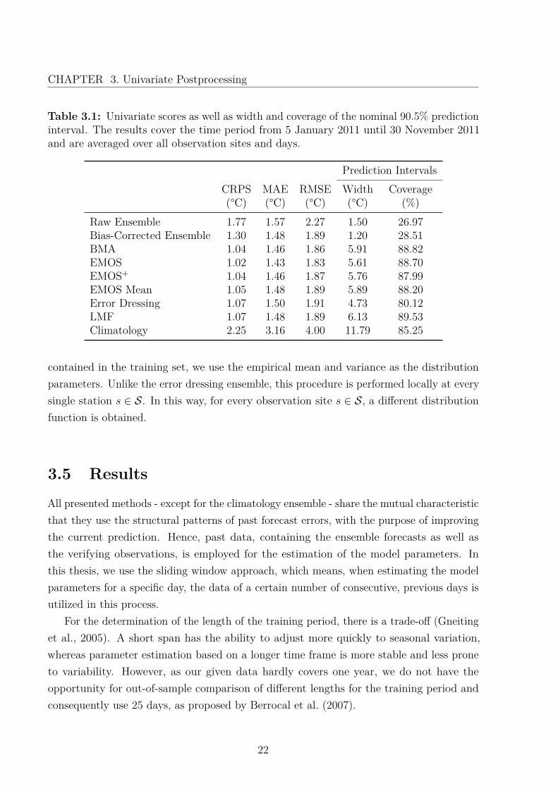
Table 3.1: Univariate scores as well as width and coverage of the nominal 90.5% predictioninterval. The results cover the time period from 5 January 2011 until 30 November 2011and are averaged over all observation sites and days.
Prediction IntervalsCRPS MAE RMSE Width Coverage(°C) (°C) (°C) (°C) (%)
Raw Ensemble 1.77 1.57 2.27 1.50 26.97Bias-Corrected Ensemble 1.30 1.48 1.89 1.20 28.51BMA 1.04 1.46 1.86 5.91 88.82EMOS 1.02 1.43 1.83 5.61 88.70EMOS+ 1.04 1.46 1.87 5.76 87.99EMOS Mean 1.05 1.48 1.89 5.89 88.20Error Dressing 1.07 1.50 1.91 4.73 80.12LMF 1.07 1.48 1.89 6.13 89.53Climatology 2.25 3.16 4.00 11.79 85.25
contained in the training set, we use the empirical mean and variance as the distributionparameters. Unlike the error dressing ensemble, this procedure is performed locally at everysingle station s ∈ S. In this way, for every observation site s ∈ S, a different distributionfunction is obtained.
3.5 Results
All presented methods - except for the climatology ensemble - share the mutual characteristicthat they use the structural patterns of past forecast errors, with the purpose of improvingthe current prediction. Hence, past data, containing the ensemble forecasts as well asthe verifying observations, is employed for the estimation of the model parameters. Inthis thesis, we use the sliding window approach, which means, when estimating the modelparameters for a specific day, the data of a certain number of consecutive, previous days isutilized in this process.
For the determination of the length of the training period, there is a trade-off (Gneitinget al., 2005). A short span has the ability to adjust more quickly to seasonal variation,whereas parameter estimation based on a longer time frame is more stable and less proneto variability. However, as our given data hardly covers one year, we do not have theopportunity for out-of-sample comparison of different lengths for the training period andconsequently use 25 days, as proposed by Berrocal et al. (2007).
22
CHAPTER 3. Univariate Postprocessing
When implementing the introduced procedures, we use the output of COSMO-DE-EPS,presented in Chapter 2. Forecast of 21h-ahead surface temperature are available from 10December 2010 until 30 November 2011. With a 25-day training period, we begin forecastingon 5 January 2011.
For the assessment of the forecasting performance, we evaluate the predictive densitiesof the competing models with the techniques presented in Appendix A. In the case of theraw and the bias-corrected ensemble, we replace the output with a normal distribution,whose parameters are the empirical mean and variance of the respective ensemble.
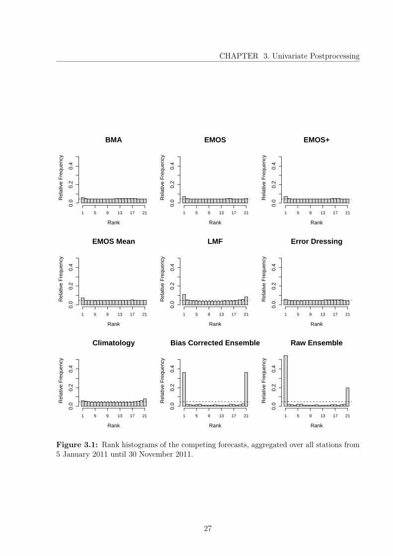
Figure 3.1 shows the rank histograms, which are based on samples of the ensemble size20 for all postprocessing models. The raw as well as the bias-corrected ensemble show aU-shape and thus underestimate the forecasting uncertainty. The remaining postprocessingtechniques correct this flaw, demonstrated by nearly uniformly appearing histograms. Thescores in Table 3.1 confirm the improvement achieved by postprocessing. Considering theCRPS, EMOS performs best, closely followed by BMA and EMOS+. Due to the highcorrelation of the forecast errors between the members of the COSMO-DE-EPS (see Chapter2), the performance of EMOS mean is very good in comparison to the more sophisticatedmodels. The subsequent methods, the LMF and the error dressing ensemble, althoughbeing simple, yield very good results. When viewing the scores, the climatology performsworst, as it is not based on predictions, but only past observations.
For the MAE and the RMSE, all postprocessed models yield comparable results, whichis to be expected as the respective predictive means are based on estimations via leastsquares regression. In terms of deterministic forecasts, the raw and climatology ensembleproduce poor results reflected in a rather high MAE and RMSE.
Again, Table 3.1 confirms the underestimated spread of the raw and bias-correctedensemble, not even covering 30% for a nominal 19/21 ≈ 90.5% prediction interval. Mostof the other techniques fulfill the requirement nearly or entirely, while still creating muchsharper forecasts than climatology. The average width of the prediction interval by theclimatology ensemble is rather large, since the variation in temperature observed in theprevious 25 days is prone to high variability.
3.6 Extension: EMOS with Student’s t-distribution
As the pre-operational phase of COSMO-DE-EPS only started in December 2010, at thebeginning of working on this thesis soley small data sets were available. The first one
23
CHAPTER 3. Univariate Postprocessing
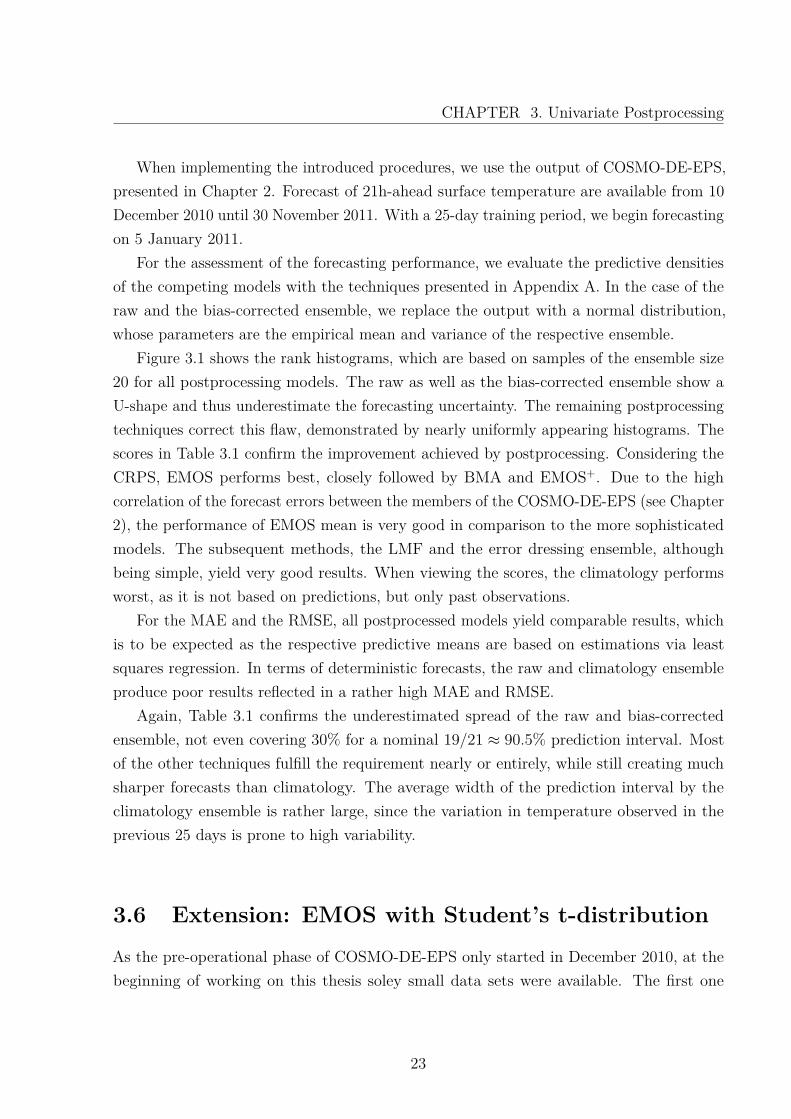
Table 3.2: Scores in degrees Celsius for different EMOS based forecasts, averaged over thetime from 5 January 2011 until 30 March 2011 and all observational sites. EMOS normalis based on a normal distribution. EMOS Student’s t employs a Student’s distributionwith different degrees of freedom ν, but uses the parameters a, b, c, d, estimated by EMOSnormal.
Model CRPS MAE RMSEEMOS normal 1.06 1.48 1.90EMOS Student’s t; ν = 3 1.09 1.48 1.90EMOS Student’s t; ν = 5 1.07 1.48 1.90EMOS Student’s t; ν = 100 1.06 1.48 1.90
comprised observations and forecasts for the time frame from 9 December 2011 until 31March 2011.
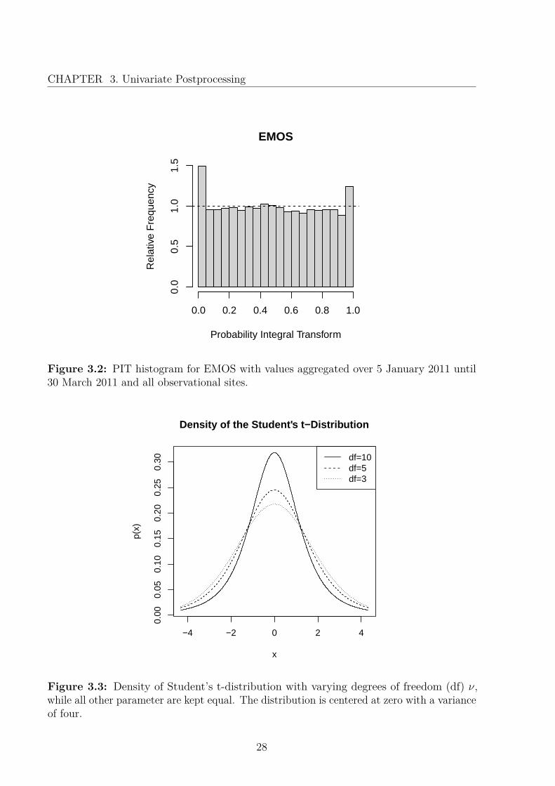
After applying EMOS to the data of this period, the forecasts were not calibrated, ascan be seen in Figure 3.2. The middle section of the probability integral transform (PIT)histogram (see Appendix A) appears almost uniform. However, many observations obtainvery low and high PIT values, which might mean that the probability mass on the edgesof the density is too small, suggesting that the normal distribution is not the best fit todescribe the predictive distribution of temperature. This particular pattern with uniformityin the middle, but outliers at the sides might be attributed to the fact that the tails of thenormal distribution are too small. In order to address this phenomenon, we study the useof the Student’s t-distribution, developed by Gosset (1908), which is an extension of thenormal distribution with heavier tails. For simplicity, we fit the Student’s t-distributionwithin an EMOS mean setting.
The density function of the Student’s t-distribution equals
p(y) =Γ(ν+1
2
)Γ(ν2
) (νπ)−12
(1 + y2
ν
)− ν+12
, (3.1)
where ν denotes the degrees of freedom and Γ the Gamma function. The parameter νdetermines the shape of the tails, as can be seen in Figure 3.3. For ν →∞, the Student’s tdensity function converges to the normal density function.
We expand the density in Equation 3.1 by introducing a scale parameter λ and a locationparameter µ (see e.g. Bishop (2006)). Then, the density is
24
CHAPTER 3. Univariate Postprocessing
p(y|µ, λ, ν) =Γ(ν+1
2
)Γ(ν2
) (λ
νπ
) 12(
1 + λ (y − µ)2
ν
)− ν+12
,
with E (y) = µ, for ν > 1, and Var(y) = 1λ
νν−2 , for ν > 2.
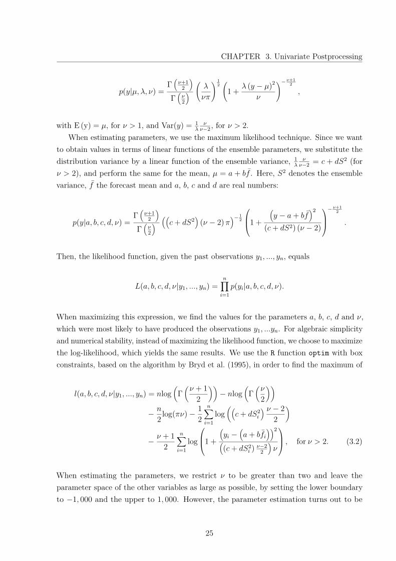
When estimating parameters, we use the maximum likelihood technique. Since we wantto obtain values in terms of linear functions of the ensemble parameters, we substitute thedistribution variance by a linear function of the ensemble variance, 1
λνν−2 = c + dS2 (for
ν > 2), and perform the same for the mean, µ = a + bf . Here, S2 denotes the ensemblevariance, f the forecast mean and a, b, c and d are real numbers:
p(y|a, b, c, d, ν) =Γ(ν+1
2
)Γ(ν2
) ((c+ dS2
)(ν − 2) π
)− 12
1 +
(y − a+ bf
)2
(c+ dS2) (ν − 2)
− ν+1
2
.
Then, the likelihood function, given the past observations y1, ..., yn, equals
L(a, b, c, d, ν|y1, ..., yn) =n∏i=1
p(yi|a, b, c, d, ν).
When maximizing this expression, we find the values for the parameters a, b, c, d and ν,which were most likely to have produced the observations y1, ...yn. For algebraic simplicityand numerical stability, instead of maximizing the likelihood function, we choose to maximizethe log-likelihood, which yields the same results. We use the R function optim with boxconstraints, based on the algorithm by Bryd et al. (1995), in order to find the maximum of
l(a, b, c, d, ν|y1, ..., yn) = nlog(
Γ(ν + 1
2
))− nlog
(Γ(ν
2
))− n
2 log(πν)− 12
n∑i=1
log((c+ dS2
i
) ν − 22
)
− ν + 12
n∑i=1
log
1 +
(yi −
(a+ bfi
))2((c+ dS2
i ) ν−22
)ν
, for ν > 2. (3.2)
When estimating the parameters, we restrict ν to be greater than two and leave theparameter space of the other variables as large as possible, by setting the lower boundaryto −1, 000 and the upper to 1, 000. However, the parameter estimation turns out to be
25
CHAPTER 3. Univariate Postprocessing
unstable, as c and d usually take unrealistic values over 20 and the estimates for ν arealways as close to two as possible.
In order to stabilize the parameter estimation, we try another approach, which mightseem suboptimal. However, if the small tails of the normal density function are the issue,this method nevertheless should detect it. We estimate the parameters a, b, c and d in theregular EMOS setting, by minimizing the CRPS for the normal density function. Then, weplug the results for a, b, c and d into Equation 3.2, so that it depends only on ν. In the finalstep, we estimate ν separately via maximum likelihood estimation of this equation. Forthis step, we again use the R function optim with box constraints, in order to regulate theparameter space for ν. If small tails caused the issue, ν ought to take small values. However,we find that ν always takes values as close to the upper boundary of the constraint aspossible. For these large values of ν, the normal and Student’s t density function coincideempirically.
In Table 3.2, we follow the aforementioned approach and then force ν to take thevalues of three, five, and hundred. The results show that there is no improvement whenmodeling with heavier tails. Instead, the CRPS, which addresses calibration and sharpnesssimultaneously, is higher for small values of ν and then decreases as ν is assigned greatervalues.
Hence, the normal density function captures the predictive distribution of temperaturebetter and other aspects must cause the structure of the PIT histogram in Figure 3.2. Itmight be attributed to the small amount of data, or due to a spatial pattern, which can notbe captured by the global parameters of EMOS. However, after receiving larger data sets,we found that the population of the outer bins in the PIT histogram decreased noticeablyand we stopped investigating this problem further.
In this chapter, we have presented different approaches for postprocessing of temperature.Most of them yield calibrated and sharp forecasts, by utilizing the structural patternsof past errors for the predictions. However, these procedures do not account for spatialcorrelation between these errors. This issue we will discuss in the succeeding chapter.
26
CHAPTER 3. Univariate Postprocessing
BMA
Rank
Rel
ativ
e F
requ
ency
0.0
0.2
0.4
1 5 9 13 17 21
EMOS
Rank
Rel
ativ
e F
requ
ency
0.0
0.2
0.4
1 5 9 13 17 21
EMOS+
Rank
Rel
ativ
e F
requ
ency
0.0
0.2
0.4
1 5 9 13 17 21
EMOS Mean
Rank
Rel
ativ
e F
requ
ency
0.0
0.2
0.4
1 5 9 13 17 21
LMF
Rank
Rel
ativ
e F
requ
ency
0.0
0.2
0.4
1 5 9 13 17 21
Error Dressing
Rank
Rel
ativ
e F
requ
ency
0.0
0.2
0.4
1 5 9 13 17 21
Climatology
Rank
Rel
ativ
e F
requ
ency
0.0
0.2
0.4
1 5 9 13 17 21
Bias Corrected Ensemble
Rank
Rel
ativ
e F
requ
ency
0.0
0.2
0.4
1 5 9 13 17 21
Raw Ensemble
Rank
Rel
ativ
e F
requ
ency
0.0
0.2
0.4
1 5 9 13 17 21
Figure 3.1: Rank histograms of the competing forecasts, aggregated over all stations from5 January 2011 until 30 November 2011.
27
CHAPTER 3. Univariate Postprocessing
EMOS
Probability Integral Transform
Rel
ativ
e F
requ
ency
0.0 0.2 0.4 0.6 0.8 1.0
0.0
0.5
1.0
1.5
Figure 3.2: PIT histogram for EMOS with values aggregated over 5 January 2011 until30 March 2011 and all observational sites.
−4 −2 0 2 4
0.00
0.05
0.10
0.15
0.20
0.25
0.30
x
p(x)
Density of the Student's t−Distribution
df=10df=5df=3
Figure 3.3: Density of Student’s t-distribution with varying degrees of freedom (df) ν,while all other parameter are kept equal. The distribution is centered at zero with a varianceof four.
28
Chapter 4
Spatial Postprocessing
This chapter focuses on different models for spatial postprocessing of ensemble temperatureforecasts. We start with a summary of the GOP method for point predictions. By modelingthe spatial correlation structure, this technique produces sharp and calibrated forecasts forentire weather fields. When combining this procedure with EMOS or BMA, introduced inChapter 3, we additionally include the information of the ensemble, while still incorporatingthe spatial structure of the weather field. Subsequently, we present two multivariatereference forecasts, ensemble copula coupling (ECC) and the noise ensemble, ending with adiscussion of the application of all techniques to COSMO-DE-EPS.
4.1 Geostatistical Output Perturbation (GOP)
Originally not developed for ensemble outputs, GOP produces sharp and calibrated forecasts,based on one deterministic prediction for weather fields. The technique consists of dressingthe multidimensional output of the numerical forecast systems with simulated error fieldsdescribed by a spatial random process. Thus, GOP perturbates the outputs of numericalweather prediction models, instead of its inputs.
Gel et al. (2004) chose to employ a parametric, stationary, and isotropic geostatisticalmodel, in order to capture the spatial structure of the error fields. The error is defined asthe difference between the observation and the bias-corrected forecast. Suppose S denotesall locations for which forecasts are available. Then, let Y = {ys : s ∈ S} be the vectorthat describes the weather variable of interest at site s ∈ S. Further, Fm = {fms : s ∈ S}refers to the weather field forecast by the member m of the ensemble with size M . Note
29
CHAPTER 4. Spatial Postprocessing
that this procedure is performed for only one member, although we include the subscriptfor future incorporation of ensemble information.
GOP is based on a statistical model, stating that
Y|Fm ∼MVN (am1 + bmFm,Σm) ,
where 1 is a vector of length #S with all entries equal to 1. Given the forecasts Fm,Y is multivariate normally distributed with mean equal to the bias corrected forecast,am1 + bmFm and the covariance matrix Σm. The entries of Σm depend on the covariancestructure of the error fields. Let C (s1, s2) be a stationary and isotropic correlation function,then the entry (i, j) of Σm equals
ρ2mδij + τ 2
m C (si, sj) ,
where δij denotes to the Kronecker delta function. The nugget effect ρ2m ≥ 0 has two
interpretations. On one hand, it can be thought of as the variance of the measurementerror. On the other hand, it is a measure of the spatial variation within a distance smallerthan the smallest distance between two different sites si and sj , for i 6= j. The sum ρ2
m + τ 2m
is called the sill.There are various ways to model the spatial structure of the weather field with different
covariance classes. Gel et al. (2004) suggest the use of the exponential correlation function,
C(si, sj) = e−||si−sj ||rm ,
where || · || denotes the Euclidean norm and the range rm > 0 is a parameter in the unitof the distance and determines the rate at which the spatial correlation decays. We alsopropose a more general approach, where we apply the Matérn correlation function (Matérn,1986)
C(si, sj) = 121−νmΓ (νm) ·
(||si − sj||
rm
)νm·Kνm
(||sj − si||
rm
).
Here, Γ(·) denotes the gamma distribution and Kν(·) the modified Bessel function of orderν > 0. The parameter ν regulates the smoothness of the simulated error field. For ν = 1
2 ,the Matérn correlation function coincides with the exponential model above.
30
CHAPTER 4. Spatial Postprocessing
The value of Y|Fm can also be calculated in terms of realizations of the error field whichmay be decomposed into two parts E1m = {ε1m(s) : s ∈ S} and E2m = {ε2m(s) : s ∈ S}(Berrocal et al., 2007):
Y|Fm = am1 + bmFm + E1m + E2m.
The vectors E1m and E2m have a multivariate distribution with mean zero and a covariancestructure based on
cov[ε1m(si), ε1m(sj)] = τ 2k C (si, sj)
andcov[ε2m(si), ε2m(sj)] = ρ2
mkδij,
respectively. The term E1m is referred to as the continuous component of the error fieldwhich varies in space, whereas E2m describes the discontinuous part, as it models a randomnoise in order to correct measurement errors.
By using the GOP method, an ensemble of any desired size can be obtained. A newmember is produced by dressing the bias corrected forecast am1+bmFm with a simulation ofthe error fields E1m and E2m. For this simulation we employ the R package RandomFieldsby Schlather (2011).
When estimating the parameters, we use a set of training data which contains pastforecasts and realized observations. There are several ways to estimate the parameters ofthe geostatistical model. Gel et al. (2004) mention a fully Bayesian approach, maximumlikelihood, and a variogram-based estimation. In order to reduce computational time, theauthors chose the last mentioned. Here, we also include a maximum likelihood approach.Independently of the estimation technique for the geostatistical model, the coefficients amand bm are estimated via linear least squares regression over the sliding training period.
In geostatistics, a variogram is a tool which describes the spatial correlation of astochastic process. Theoretically, it is defined as
γm (si, sj) = 12Var (X(si)−X(sj)) ,
where X(s) denotes the value of the stochastic process at location s. Since the underlyingmodel of the GOP method is stationary, the variogram reduces to a function that dependson the distance d = ||si − sj|| only. Additionally, the mean and the variance of the error
31
CHAPTER 4. Spatial Postprocessing
fields are defined as spatially constant so that the theoretical variogram values γ(d) of thegeostatistical model equal
γm(d) = ρ2mδij + τ 2
m (1− C (si, sj)) ,
see e.g. Diggle and Ribeiro Jr. (2007).For the estimation of the parameters, we calculate an empirical version of the variogram
following the approach by Berrocal et al. (2007). After determining am and bm, we computethe errors, which equal the residuals of the linear least squares regression fit. For each day inthe training period, we then determine the distances between every possible pair of locations.Additionally, we calculate one-half the squared difference between the corresponding pair oferrors,
12(esi − esj
)2,
where esi and esj denote the site-specific errors on one day in the training period. In thefollowing step, the collection of distances are sorted into bins Bl with centers at dl. The cutpoints of the bins are chosen by the rule that on average during the entire forecasting period,the same amount of distances should fall in every bin. During the entire forecasting period,the cut points and centers stay constant, as implemented in the R package ProbForecastGOPby Berrocal et al. (2010). Finally, the empirical variogram value γm(dl) at distance dl equalsthe average of one-half the squared difference of the errors whose distances fall into bin Bl.
When fitting a curve to the empirical variogram values, Berrocal et al. (2007) employweighted least squares as proposed by Cressie (1985). Let θm denote the parameter vectorwhich depends on ρ2
m, τ 2m and rm, in the case of an exponential correlation function, and
additionally on ν for a Matérn model. In order to obtain the optimal value of θm, thefunction
S(θm) =∑l
nlγm(xl)− γ(θm, dl)
γ(θm, dl)
is minimized. Here, nl refers to the number of pairs contained in bin Bl. When minimizingthe expression, we employ the R function optim with boundary conditions based on thealgorithm by Bryd et al. (1995).
Beside the variogram-based estimation, we also apply a maximum likelihood approach.Since the errors are assumed to be a realization of a Gaussian random field, the likelihoodfunction is
L(θm, em) = 1(2π)n/2 |∑(θm)|1/2
e−12 em
∑(θm)−1etm ,
32
CHAPTER 4. Spatial Postprocessing
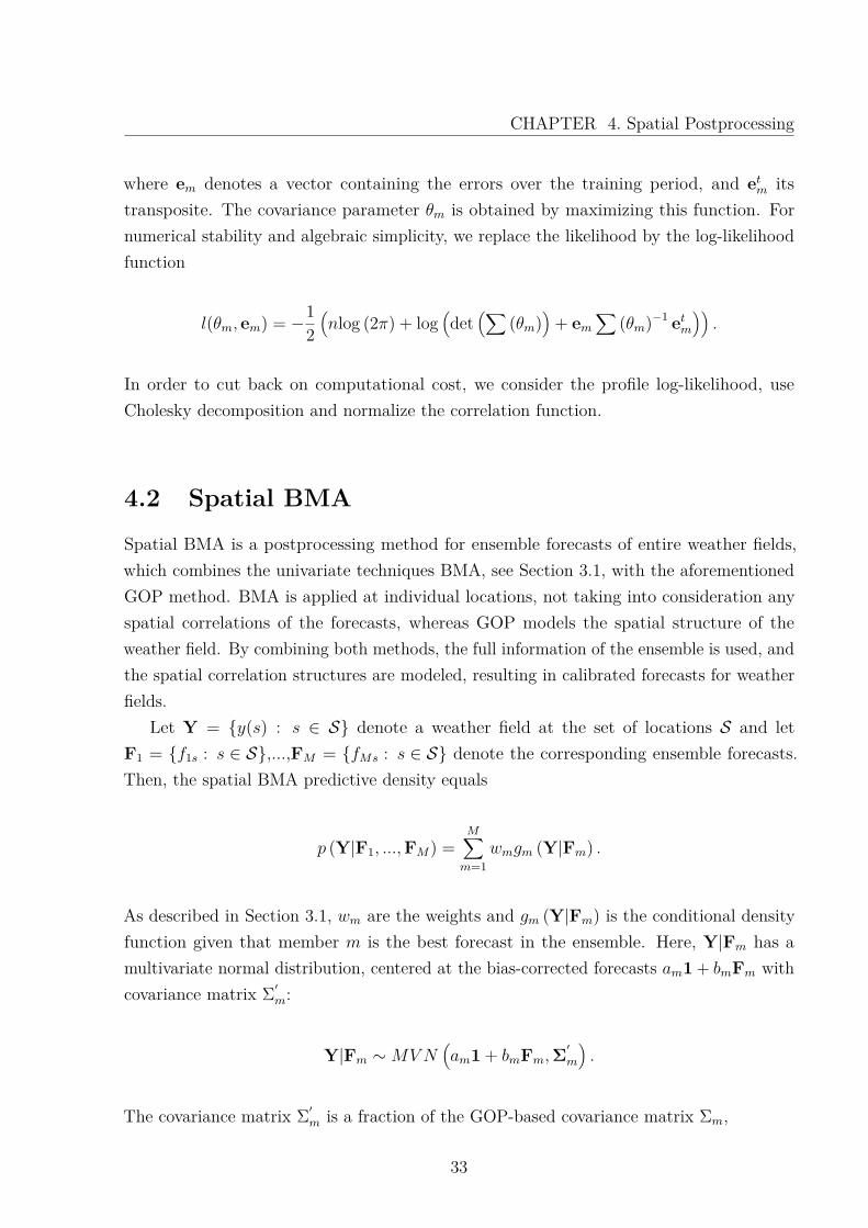
where em denotes a vector containing the errors over the training period, and etm itstransposite. The covariance parameter θm is obtained by maximizing this function. Fornumerical stability and algebraic simplicity, we replace the likelihood by the log-likelihoodfunction
l(θm, em) = −12(nlog (2π) + log
(det
(∑(θm)
)+ em
∑(θm)−1 etm
)).
In order to cut back on computational cost, we consider the profile log-likelihood, useCholesky decomposition and normalize the correlation function.
4.2 Spatial BMA
Spatial BMA is a postprocessing method for ensemble forecasts of entire weather fields,which combines the univariate techniques BMA, see Section 3.1, with the aforementionedGOP method. BMA is applied at individual locations, not taking into consideration anyspatial correlations of the forecasts, whereas GOP models the spatial structure of theweather field. By combining both methods, the full information of the ensemble is used, andthe spatial correlation structures are modeled, resulting in calibrated forecasts for weatherfields.
Let Y = {y(s) : s ∈ S} denote a weather field at the set of locations S and letF1 = {f1s : s ∈ S},...,FM = {fMs : s ∈ S} denote the corresponding ensemble forecasts.Then, the spatial BMA predictive density equals
p (Y|F1, ...,FM) =M∑m=1
wmgm (Y|Fm) .
As described in Section 3.1, wm are the weights and gm (Y|Fm) is the conditional densityfunction given that member m is the best forecast in the ensemble. Here, Y|Fm has amultivariate normal distribution, centered at the bias-corrected forecasts am1 + bmFm withcovariance matrix Σ′m:
Y|Fm ∼MVN(am1 + bmFm,Σ
′
m
).
The covariance matrix Σ′m is a fraction of the GOP-based covariance matrix Σm,
33
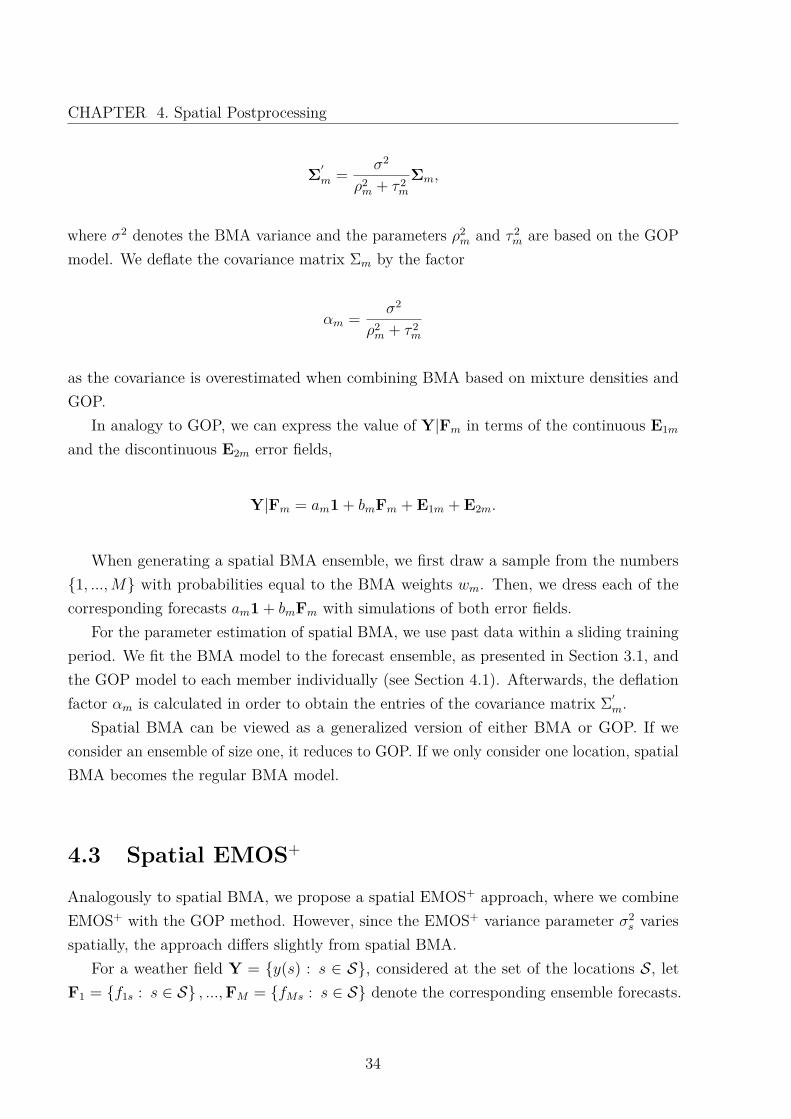
CHAPTER 4. Spatial Postprocessing
Σ′m = σ2
ρ2m + τ 2
m
Σm,
where σ2 denotes the BMA variance and the parameters ρ2m and τ 2
m are based on the GOPmodel. We deflate the covariance matrix Σm by the factor
αm = σ2
ρ2m + τ 2
m
as the covariance is overestimated when combining BMA based on mixture densities andGOP.
In analogy to GOP, we can express the value of Y|Fm in terms of the continuous E1m
and the discontinuous E2m error fields,
Y|Fm = am1 + bmFm + E1m + E2m.
When generating a spatial BMA ensemble, we first draw a sample from the numbers{1, ...,M} with probabilities equal to the BMA weights wm. Then, we dress each of thecorresponding forecasts am1 + bmFm with simulations of both error fields.
For the parameter estimation of spatial BMA, we use past data within a sliding trainingperiod. We fit the BMA model to the forecast ensemble, as presented in Section 3.1, andthe GOP model to each member individually (see Section 4.1). Afterwards, the deflationfactor αm is calculated in order to obtain the entries of the covariance matrix Σ′m.
Spatial BMA can be viewed as a generalized version of either BMA or GOP. If weconsider an ensemble of size one, it reduces to GOP. If we only consider one location, spatialBMA becomes the regular BMA model.
4.3 Spatial EMOS+
Analogously to spatial BMA, we propose a spatial EMOS+ approach, where we combineEMOS+ with the GOP method. However, since the EMOS+ variance parameter σ2
s variesspatially, the approach differs slightly from spatial BMA.
For a weather field Y = {y(s) : s ∈ S}, considered at the set of the locations S, letF1 = {f1s : s ∈ S} , ...,FM = {fMs : s ∈ S} denote the corresponding ensemble forecasts.
34
CHAPTER 4. Spatial Postprocessing
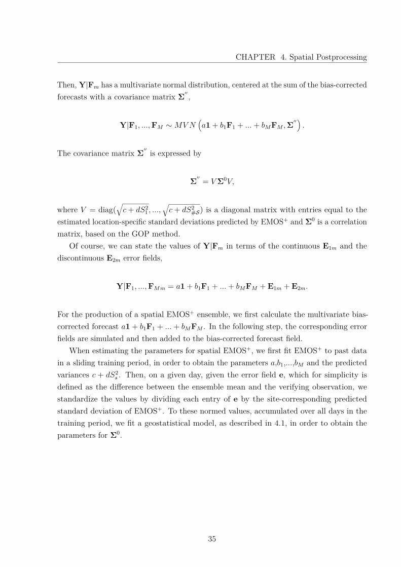
Then, Y|Fm has a multivariate normal distribution, centered at the sum of the bias-correctedforecasts with a covariance matrix Σ′′ ,
Y|F1, ...,FM ∼MVN(a1 + b1F1 + ...+ bMFM ,Σ
′′).
The covariance matrix Σ′′ is expressed by
Σ′′ = VΣ0V,
where V = diag(√c+ dS2
1 , ...,√c+ dS2
#S) is a diagonal matrix with entries equal to theestimated location-specific standard deviations predicted by EMOS+ and Σ0 is a correlationmatrix, based on the GOP method.
Of course, we can state the values of Y|Fm in terms of the continuous E1m and thediscontinuous E2m error fields,
Y|F1, ...,FMm = a1 + b1F1 + ...+ bMFM + E1m + E2m.
For the production of a spatial EMOS+ ensemble, we first calculate the multivariate bias-corrected forecast a1 + b1F1 + ...+ bMFM . In the following step, the corresponding errorfields are simulated and then added to the bias-corrected forecast field.
When estimating the parameters for spatial EMOS+, we first fit EMOS+ to past datain a sliding training period, in order to obtain the parameters a,b1,...,bM and the predictedvariances c + dS2
s . Then, on a given day, given the error field e, which for simplicity isdefined as the difference between the ensemble mean and the verifying observation, westandardize the values by dividing each entry of e by the site-corresponding predictedstandard deviation of EMOS+. To these normed values, accumulated over all days in thetraining period, we fit a geostatistical model, as described in 4.1, in order to obtain theparameters for Σ0.
35

CHAPTER 4. Spatial Postprocessing
4.4 Reference Forecasts
Ensemble Copula Coupling (ECC)
ECC, proposed by Schefzik (2011), is a multivariate postprocessing technique for ensembleforecasts. Based on existing univariate postprocessing methods, ECC models the multivari-ate dependency structure of the forecasts by incorporating the multivariate rank structureof the original ensemble through a discrete copula. In the current context, we employ ECCbased on BMA and EMOS+, discussed in Chapter 3. When generating the ECC forecasts,we proceed according to the following steps:
1. Univariate postprocessing
First, we apply any available postprocessing method to the ensemble output, inorder to produce a calibrated predictive distribution. Subsequently, for each locations ∈ S, we draw a random sample f1s, ..., fMs of the original ensemble size M fromthis distribution.
2. Combining the results of step 1 with the ensemble’s dependency structure
Given the ensemble forecasts f1s, ..., fMs, we denote their ranks ω(s, 1), ..., ω(s,M) ateach station. Then, we sort the random sample according to the ensemble’s orderstatistic: fω(s,1), ..., fω(s,M). Finally, one member m of the ECC ensemble equals thevector (fω(1,m), ..., fω(#S,m)).
If a larger ensemble is desired, the steps may be repeated n ∈ N times, in order to generatean ensemble of the size nM . ECC provides an easy technique, which in our case producesspatially consistent forecast fields by inheriting the dependence structure of the originalensemble.
Noise Ensemble
In order to account for measurement errors or small scale spatial variations, we includethe noise ensemble, which was also considered in Berrocal et al. (2007). To each memberm of the raw ensemble, we add a Gaussian noise with mean zero and a variance equal tothe corresponding nugget effect ρ2
m. This task is performed independently at each location.Thus, the noise ensemble does not capture the spatial structure of the weather field, butincludes patterns of past site-specific errors, in order to improve the forecasts.
36
CHAPTER 4. Spatial Postprocessing
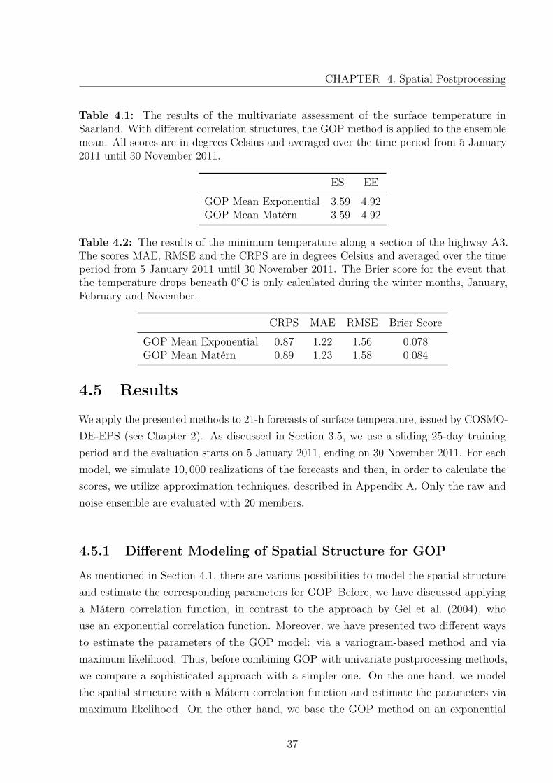
Table 4.1: The results of the multivariate assessment of the surface temperature inSaarland. With different correlation structures, the GOP method is applied to the ensemblemean. All scores are in degrees Celsius and averaged over the time period from 5 January2011 until 30 November 2011.
ES EEGOP Mean Exponential 3.59 4.92GOP Mean Matérn 3.59 4.92
Table 4.2: The results of the minimum temperature along a section of the highway A3.The scores MAE, RMSE and the CRPS are in degrees Celsius and averaged over the timeperiod from 5 January 2011 until 30 November 2011. The Brier score for the event thatthe temperature drops beneath 0°C is only calculated during the winter months, January,February and November.
CRPS MAE RMSE Brier ScoreGOP Mean Exponential 0.87 1.22 1.56 0.078GOP Mean Matérn 0.89 1.23 1.58 0.084
4.5 Results
We apply the presented methods to 21-h forecasts of surface temperature, issued by COSMO-DE-EPS (see Chapter 2). As discussed in Section 3.5, we use a sliding 25-day trainingperiod and the evaluation starts on 5 January 2011, ending on 30 November 2011. For eachmodel, we simulate 10, 000 realizations of the forecasts and then, in order to calculate thescores, we utilize approximation techniques, described in Appendix A. Only the raw andnoise ensemble are evaluated with 20 members.
4.5.1 Different Modeling of Spatial Structure for GOP
As mentioned in Section 4.1, there are various possibilities to model the spatial structureand estimate the corresponding parameters for GOP. Before, we have discussed applyinga Mátern correlation function, in contrast to the approach by Gel et al. (2004), whouse an exponential correlation function. Moreover, we have presented two different waysto estimate the parameters of the GOP model: via a variogram-based method and viamaximum likelihood. Thus, before combining GOP with univariate postprocessing methods,we compare a sophisticated approach with a simpler one. On the one hand, we modelthe spatial structure with a Mátern correlation function and estimate the parameters viamaximum likelihood. On the other hand, we base the GOP method on an exponential
37
CHAPTER 4. Spatial Postprocessing
GOP Exponential
Rank
Rel
ativ
e F
requ
ency
0.00
0.04
0.08
1 5 9 13 17 21
GOP Matérn
RankR
elat
ive
Fre
quen
cy
0.00
0.04
0.08
1 5 9 13 17 21
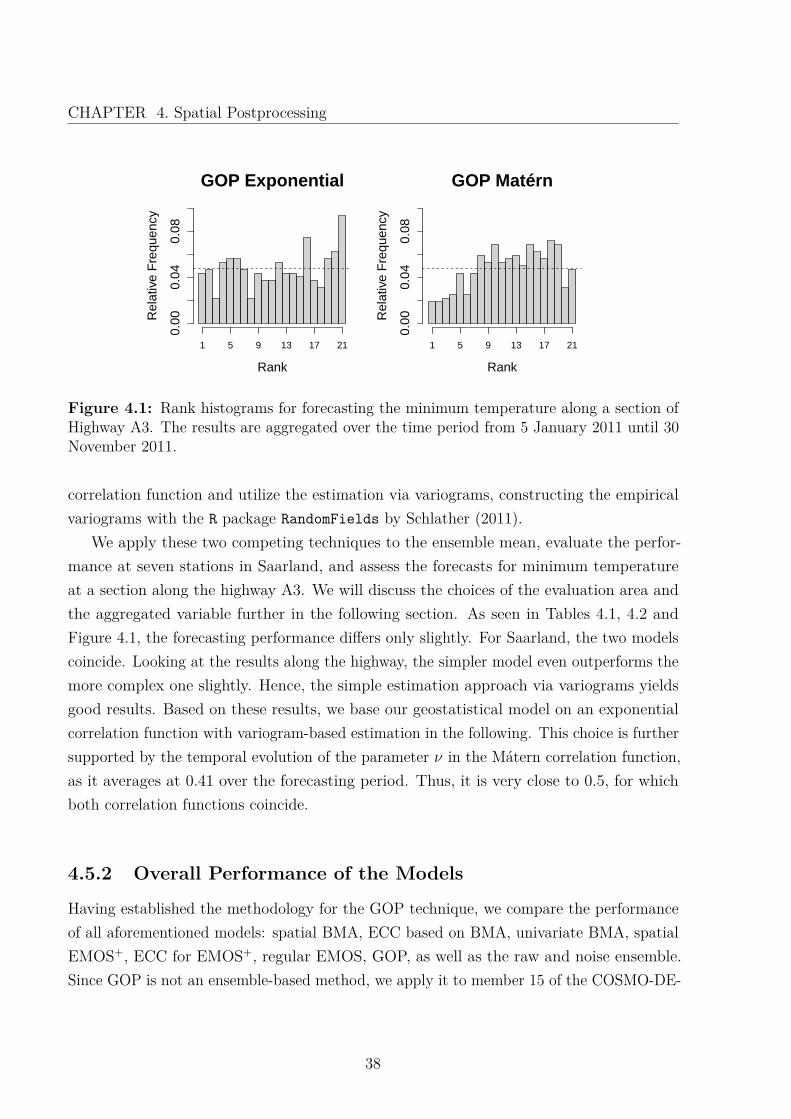
Figure 4.1: Rank histograms for forecasting the minimum temperature along a section ofHighway A3. The results are aggregated over the time period from 5 January 2011 until 30November 2011.
correlation function and utilize the estimation via variograms, constructing the empiricalvariograms with the R package RandomFields by Schlather (2011).
We apply these two competing techniques to the ensemble mean, evaluate the perfor-mance at seven stations in Saarland, and assess the forecasts for minimum temperatureat a section along the highway A3. We will discuss the choices of the evaluation area andthe aggregated variable further in the following section. As seen in Tables 4.1, 4.2 andFigure 4.1, the forecasting performance differs only slightly. For Saarland, the two modelscoincide. Looking at the results along the highway, the simpler model even outperforms themore complex one slightly. Hence, the simple estimation approach via variograms yieldsgood results. Based on these results, we base our geostatistical model on an exponentialcorrelation function with variogram-based estimation in the following. This choice is furthersupported by the temporal evolution of the parameter ν in the Mátern correlation function,as it averages at 0.41 over the forecasting period. Thus, it is very close to 0.5, for whichboth correlation functions coincide.
4.5.2 Overall Performance of the Models
Having established the methodology for the GOP technique, we compare the performanceof all aforementioned models: spatial BMA, ECC based on BMA, univariate BMA, spatialEMOS+, ECC for EMOS+, regular EMOS, GOP, as well as the raw and noise ensemble.Since GOP is not an ensemble-based method, we apply it to member 15 of the COSMO-DE-
38
CHAPTER 4. Spatial Postprocessing
●
●●●●
●
●●●●●
●●●
●●●
●●●●●●●●
●●
●●●
●
●●
●●●●●●
●●●●
●●
●●●
●●
●●●●●
●
●
●●●●●●●●
●●●
●●●
●●●●
●●
●
●●●
●
●
●
●●●●
●●
●●
●●
●●●●●●●●●●
●●●●●●●●●●
●
●
●
●●
●●●●●●
●●●●●●●●
●
●●●●●●●●●●●●●●●●●●●
●●●●
●
●
●
●
●●●
●●●●●
●●●●
●
●
●
●●●
●●●●●
●●●
●
●●●●●●●●●
●●
●●●●●●●●●●●
●●
●●
●
●
●●●●
●
●
●●●●
●
●●
●
●●
●
●●●●●
●●●
●●●●
●
●●●●●
●●
●
●
●●●●●●●●
●
●
●
●
●
●
●●
●●
●●
●●●
●●●●
●
●●●●
●●●●
●●
●●●
●
●●●
0 100 200 300 400 500
01
23
45
Exponential
Distance
Sem
i−V
aria
nce
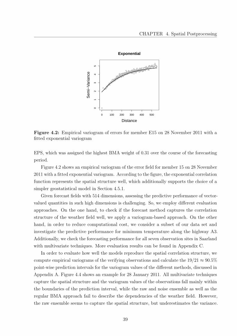
Figure 4.2: Empirical variogram of errors for member E15 on 28 November 2011 with afitted exponential variogram
EPS, which was assigned the highest BMA weight of 0.31 over the course of the forecastingperiod.
Figure 4.2 shows an empirical variogram of the error field for member 15 on 28 November2011 with a fitted exponential variogram. According to the figure, the exponential correlationfunction represents the spatial structure well, which additionally supports the choice of asimpler geostatistical model in Section 4.5.1.
Given forecast fields with 514 dimensions, assessing the predictive performance of vector-valued quantities in such high dimensions is challenging. So, we employ different evaluationapproaches. On the one hand, to check if the forecast method captures the correlationstructure of the weather field well, we apply a variogram-based approach. On the otherhand, in order to reduce computational cost, we consider a subset of our data set andinvestigate the predictive performance for minimum temperature along the highway A3.Additionally, we check the forecasting performance for all seven observation sites in Saarlandwith multivariate techniques. More evaluation results can be found in Appendix C.
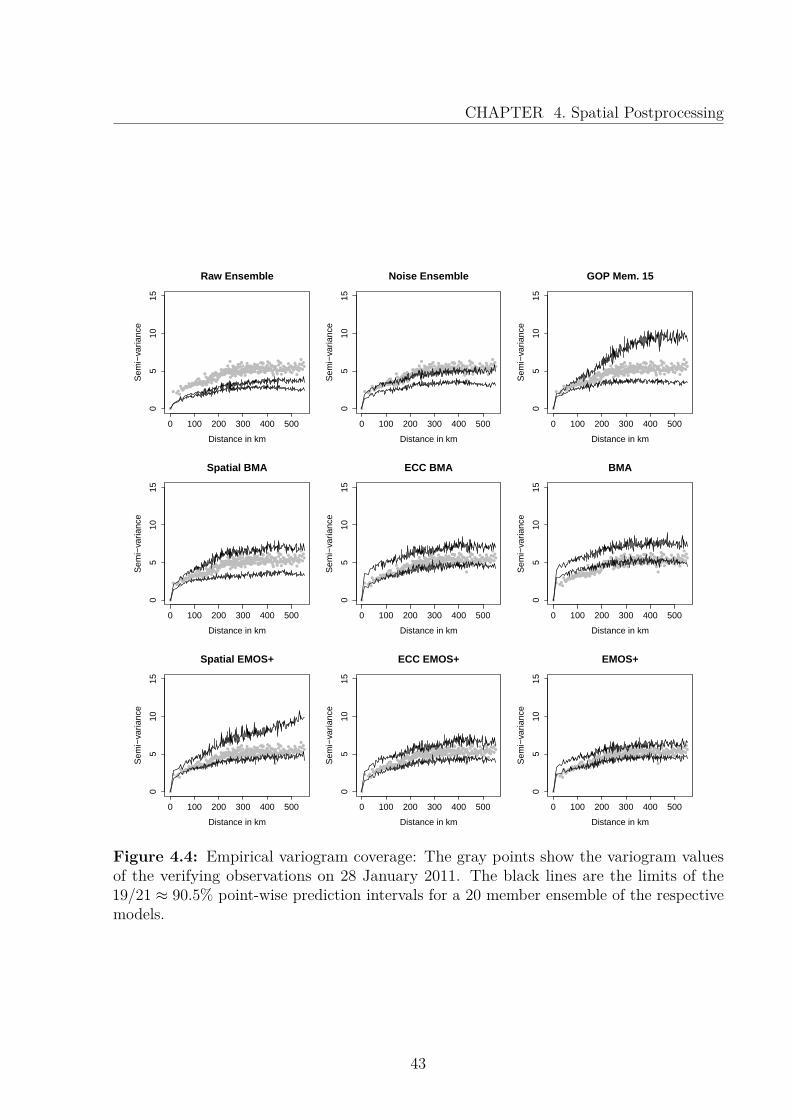
In order to evaluate how well the models reproduce the spatial correlation structure, wecompute empirical variograms of the verifying observations and calculate the 19/21 ≈ 90.5%point-wise prediction intervals for the variogram values of the different methods, discussed inAppendix A. Figure 4.4 shows an example for 28 January 2011. All multivariate techniquescapture the spatial structure and the variogram values of the observations fall mainly withinthe boundaries of the prediction interval, while the raw and noise ensemble as well as theregular BMA approach fail to describe the dependencies of the weather field. However,the raw ensemble seems to capture the spatial structure, but underestimates the variance.
39
CHAPTER 4. Spatial Postprocessing
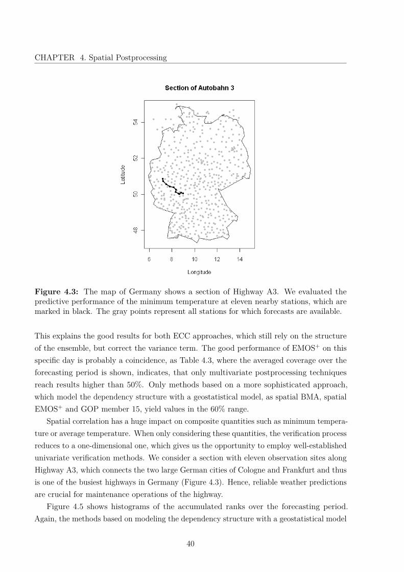
Figure 4.3: The map of Germany shows a section of Highway A3. We evaluated thepredictive performance of the minimum temperature at eleven nearby stations, which aremarked in black. The gray points represent all stations for which forecasts are available.
This explains the good results for both ECC approaches, which still rely on the structureof the ensemble, but correct the variance term. The good performance of EMOS+ on thisspecific day is probably a coincidence, as Table 4.3, where the averaged coverage over theforecasting period is shown, indicates, that only multivariate postprocessing techniquesreach results higher than 50%. Only methods based on a more sophisticated approach,which model the dependency structure with a geostatistical model, as spatial BMA, spatialEMOS+ and GOP member 15, yield values in the 60% range.
Spatial correlation has a huge impact on composite quantities such as minimum tempera-ture or average temperature. When only considering these quantities, the verification processreduces to a one-dimensional one, which gives us the opportunity to employ well-establishedunivariate verification methods. We consider a section with eleven observation sites alongHighway A3, which connects the two large German cities of Cologne and Frankfurt and thusis one of the busiest highways in Germany (Figure 4.3). Hence, reliable weather predictionsare crucial for maintenance operations of the highway.
Figure 4.5 shows histograms of the accumulated ranks over the forecasting period.Again, the methods based on modeling the dependency structure with a geostatistical model
40
CHAPTER 4. Spatial Postprocessing
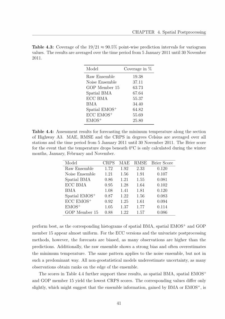
Table 4.3: Coverage of the 19/21 ≈ 90.5% point-wise prediction intervals for variogramvalues. The results are averaged over the time period from 5 January 2011 until 30 November2011.
Model Coverage in %Raw Ensemble 19.38Noise Ensemble 37.11GOP Member 15 63.73Spatial BMA 67.64ECC BMA 55.37BMA 34.40Spatial EMOS+ 64.82ECC EMOS+ 55.69EMOS+ 25.80
Table 4.4: Assessment results for forecasting the minimum temperature along the sectionof Highway A3. MAE, RMSE and the CRPS in degrees Celsius are averaged over allstations and the time period from 5 January 2011 until 30 November 2011. The Brier scorefor the event that the temperature drops beneath 0°C is only calculated during the wintermonths, January, February and November.
Model CRPS MAE RMSE Brier ScoreRaw Ensemble 1.72 1.92 2.33 0.120Noise Ensemble 1.21 1.56 1.91 0.107Spatial BMA 0.86 1.21 1.55 0.081ECC BMA 0.95 1.28 1.64 0.102BMA 1.08 1.41 1.81 0.120Spatial EMOS+ 0.87 1.22 1.56 0.083ECC EMOS+ 0.92 1.25 1.61 0.094EMOS+ 1.05 1.37 1.77 0.114GOP Member 15 0.88 1.22 1.57 0.086
perform best, as the corresponding histograms of spatial BMA, spatial EMOS+ and GOPmember 15 appear almost uniform. For the ECC versions and the univariate postprocessingmethods, however, the forecasts are biased, as many observations are higher than thepredictions. Additionally, the raw ensemble shows a strong bias and often overestimatesthe minimum temperature. The same pattern applies to the noise ensemble, but not insuch a predominant way. All non-geostatistical models underestimate uncertainty, as manyobservations obtain ranks on the edge of the ensemble.
The scores in Table 4.4 further support these results, as spatial BMA, spatial EMOS+
and GOP member 15 yield the lowest CRPS scores. The corresponding values differ onlyslightly, which might suggest that the ensemble information, gained by BMA or EMOS+, is
41
CHAPTER 4. Spatial Postprocessing
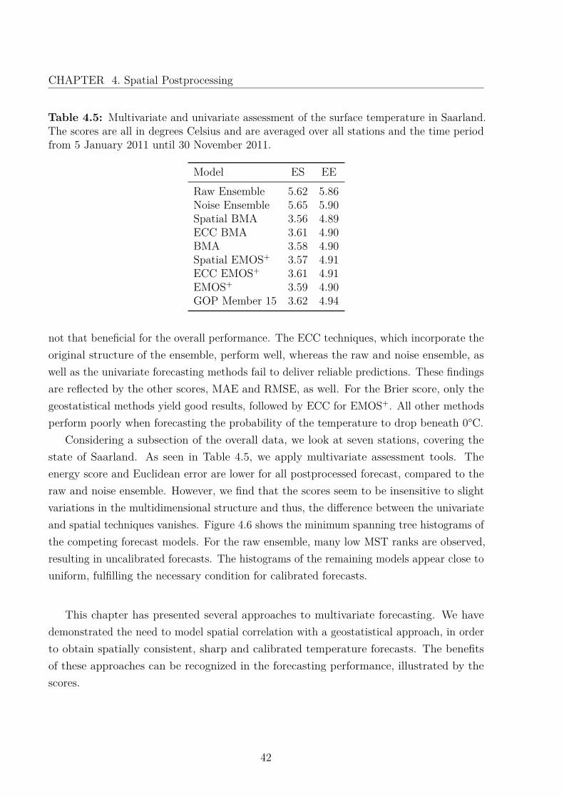
Table 4.5: Multivariate and univariate assessment of the surface temperature in Saarland.The scores are all in degrees Celsius and are averaged over all stations and the time periodfrom 5 January 2011 until 30 November 2011.
Model ES EERaw Ensemble 5.62 5.86Noise Ensemble 5.65 5.90Spatial BMA 3.56 4.89ECC BMA 3.61 4.90BMA 3.58 4.90Spatial EMOS+ 3.57 4.91ECC EMOS+ 3.61 4.91EMOS+ 3.59 4.90GOP Member 15 3.62 4.94
not that beneficial for the overall performance. The ECC techniques, which incorporate theoriginal structure of the ensemble, perform well, whereas the raw and noise ensemble, aswell as the univariate forecasting methods fail to deliver reliable predictions. These findingsare reflected by the other scores, MAE and RMSE, as well. For the Brier score, only thegeostatistical methods yield good results, followed by ECC for EMOS+. All other methodsperform poorly when forecasting the probability of the temperature to drop beneath 0°C.
Considering a subsection of the overall data, we look at seven stations, covering thestate of Saarland. As seen in Table 4.5, we apply multivariate assessment tools. Theenergy score and Euclidean error are lower for all postprocessed forecast, compared to theraw and noise ensemble. However, we find that the scores seem to be insensitive to slightvariations in the multidimensional structure and thus, the difference between the univariateand spatial techniques vanishes. Figure 4.6 shows the minimum spanning tree histograms ofthe competing forecast models. For the raw ensemble, many low MST ranks are observed,resulting in uncalibrated forecasts. The histograms of the remaining models appear close touniform, fulfilling the necessary condition for calibrated forecasts.
This chapter has presented several approaches to multivariate forecasting. We havedemonstrated the need to model spatial correlation with a geostatistical approach, in orderto obtain spatially consistent, sharp and calibrated temperature forecasts. The benefitsof these approaches can be recognized in the forecasting performance, illustrated by thescores.
42
CHAPTER 4. Spatial Postprocessing
●
●●●●
●●●●
●●●●●●
●●●●●●●●●
●●●●
●●
●
●●
●●●●●
●●●
●●●●●
●
●●
●
●●
●●
●
●
●
●●●●
●●
●
●●
●●
●
●
●
●●●●
●●
●
●
●●●
●●●●●●●●
●
●
●
●●
●●●
●●
●●●●●●●●●●
●
●●
●●
●
●
●
●
●●
●●●
●●
●
●
●●●
●●
●
●
●
●●●●●
●●●
●●●●
●●
●
●●
●
●●●
●
●●●●●●
●
●●●
●●
●
●●
●
●●
●●
●●●●
●●
●
●●●●●●
●
●
●
●●●●●●●
●
●
●
●●
●●
●●
●
●●
●
●●
●●
●●●●●●●●
●●
●
●
●●●●
●
●●●●
●
●
●●●
●●●
●
●●●●●
●
●
●
●
●
●●
●
●
●●●
●●●
●
●●●●●●
●
●●●
●●
●
●●●●
●●●
●
●●
●
●
●
●
●
●
●
●
0 100 200 300 400 500
05
1015
Raw Ensemble
Distance in km
Sem
i−va
rianc
e
●
●●●●
●●●●
●●●●●●
●●●●●●●●●
●●●●
●●
●
●●
●●●●●
●●●
●●●●●
●
●●
●
●●
●●
●
●
●
●●●●
●●
●
●●
●●
●
●
●
●●●●
●●
●
●
●●●
●●●●●●●●
●
●
●
●●
●●●
●●
●●●●●●●●●●
●
●●
●●
●
●
●
●
●●
●●●
●●
●
●
●●●
●●
●
●
●
●●●●●
●●●
●●●●
●●
●
●●
●
●●●
●
●●●●●●
●
●●●
●●
●
●●
●
●●
●●
●●●●
●●
●
●●●●●●
●
●
●
●●●●●●●
●
●
●
●●
●●
●●
●
●●
●
●●
●●
●●●●●●●●
●●
●
●
●●●●
●
●●●●
●
●
●●●
●●●
●
●●●●●
●
●
●
●
●
●●
●
●
●●●
●●●
●
●●●●●●
●
●●●
●●
●
●●●●
●●●
●
●●
●
●
●
●
●
●
●
●
0 100 200 300 400 500
05
1015
Noise Ensemble
Distance in km
Sem
i−va
rianc
e
●
●●●●
●●●●
●●●●●●
●●●●●●●●●
●●●●
●●
●
●●
●●●●●
●●●
●●●●●
●
●●
●
●●
●●
●
●
●
●●●●
●●
●
●●
●●
●
●
●
●●●●
●●
●
●
●●●
●●●●●●●●
●
●
●
●●
●●●
●●
●●●●●●●●●●
●
●●
●●
●
●
●
●
●●
●●●
●●
●
●
●●●
●●
●
●
●
●●●●●
●●●
●●●●
●●
●
●●
●
●●●
●
●●●●●●
●
●●●
●●
●
●●
●
●●
●●
●●●●
●●
●
●●●●●●
●
●
●
●●●●●●●
●
●
●
●●
●●
●●
●
●●
●
●●
●●
●●●●●●●●
●●
●
●
●●●●
●
●●●●
●
●
●●●
●●●
●
●●●●●
●
●
●
●
●
●●
●
●
●●●
●●●
●
●●●●●●
●
●●●
●●
●
●●●●
●●●
●
●●
●
●
●
●
●
●
●
●
0 100 200 300 400 500
05
1015
GOP Mem. 15
Distance in km
Sem
i−va
rianc
e
●
●●●●
●●●●
●●●●●●
●●●●●●●●●
●●●●
●●
●
●●
●●●●●
●●●
●●●●●
●
●●
●
●●
●●
●
●
●
●●●●
●●
●
●●
●●
●
●
●
●●●●
●●
●
●
●●●
●●●●●●●●
●
●
●
●●
●●●
●●
●●●●●●●●●●
●
●●
●●
●
●
●
●
●●
●●●
●●
●
●
●●●
●●
●
●
●
●●●●●
●●●
●●●●
●●
●
●●
●
●●●
●
●●●●●●
●
●●●
●●
●
●●
●
●●
●●
●●●●
●●
●
●●●●●●
●
●
●
●●●●●●●
●
●
●
●●
●●
●●
●
●●
●
●●
●●
●●●●●●●●
●●
●
●
●●●●
●
●●●●
●
●
●●●
●●●
●
●●●●●
●
●
●
●
●
●●
●
●
●●●
●●●
●
●●●●●●
●
●●●
●●
●
●●●●
●●●
●
●●
●
●
●
●
●
●
●
●
0 100 200 300 400 500
05
1015
Spatial BMA
Distance in km
Sem
i−va
rianc
e
●
●●●●
●●●●
●●●●●●
●●●●●●●●●
●●●●
●●
●
●●
●●●●●
●●●
●●●●●
●
●●
●
●●
●●
●
●
●
●●●●
●●
●
●●
●●
●
●
●
●●●●
●●
●
●
●●●
●●●●●●●●
●
●
●
●●
●●●
●●
●●●●●●●●●●
●
●●
●●
●
●
●
●
●●
●●●
●●
●
●
●●●
●●
●
●
●
●●●●●
●●●
●●●●
●●
●
●●
●
●●●
●
●●●●●●
●
●●●
●●
●
●●
●
●●
●●
●●●●
●●
●
●●●●●●
●
●
●
●●●●●●●
●
●
●
●●
●●
●●
●
●●
●
●●
●●
●●●●●●●●
●●
●
●
●●●●
●
●●●●
●
●
●●●
●●●
●
●●●●●
●
●
●
●
●
●●
●
●
●●●
●●●
●
●●●●●●
●
●●●
●●
●
●●●●
●●●
●
●●
●
●
●
●
●
●
●
●
0 100 200 300 400 500
05
1015
ECC BMA
Distance in km
Sem
i−va
rianc
e
●
●●●●
●●●●
●●●●●●
●●●●●●●●●
●●●●
●●
●
●●
●●●●●
●●●
●●●●●
●
●●
●
●●
●●
●
●
●
●●●●
●●
●
●●
●●
●
●
●
●●●●
●●
●
●
●●●
●●●●●●●●
●
●
●
●●
●●●
●●
●●●●●●●●●●
●
●●
●●
●
●
●
●
●●
●●●
●●
●
●
●●●
●●
●
●
●
●●●●●
●●●
●●●●
●●
●
●●
●
●●●
●
●●●●●●
●
●●●
●●
●
●●
●
●●
●●
●●●●
●●
●
●●●●●●
●
●
●
●●●●●●●
●
●
●
●●
●●
●●
●
●●
●
●●
●●
●●●●●●●●
●●
●
●
●●●●
●
●●●●
●
●
●●●
●●●
●
●●●●●
●
●
●
●
●
●●
●
●
●●●
●●●
●
●●●●●●
●
●●●
●●
●
●●●●
●●●
●
●●
●
●
●
●
●
●
●
●
0 100 200 300 400 500
05
1015
BMA
Distance in km
Sem
i−va
rianc
e
●
●●●●
●●●●
●●●●●●
●●●●●●●●●
●●●●
●●
●
●●
●●●●●
●●●
●●●●●
●
●●
●
●●
●●
●
●
●
●●●●
●●
●
●●
●●
●
●
●
●●●●
●●
●
●
●●●
●●●●●●●●
●
●
●
●●
●●●
●●
●●●●●●●●●●
●
●●
●●
●
●
●
●
●●
●●●
●●
●
●
●●●
●●
●
●
●
●●●●●
●●●
●●●●
●●
●
●●
●
●●●
●
●●●●●●
●
●●●
●●
●
●●
●
●●
●●
●●●●
●●
●
●●●●●●
●
●
●
●●●●●●●
●
●
●
●●
●●
●●
●
●●
●
●●
●●
●●●●●●●●
●●
●
●
●●●●
●
●●●●
●
●
●●●
●●●
●
●●●●●
●
●
●
●
●
●●
●
●
●●●
●●●
●
●●●●●●
●
●●●
●●
●
●●●●
●●●
●
●●
●
●
●
●
●
●
●
●
0 100 200 300 400 500
05
1015
Spatial EMOS+
Distance in km
Sem
i−va
rianc
e
●
●●●●
●●●●
●●●●●●
●●●●●●●●●
●●●●
●●
●
●●
●●●●●
●●●
●●●●●
●
●●
●
●●
●●
●
●
●
●●●●
●●
●
●●
●●
●
●
●
●●●●
●●
●
●
●●●
●●●●●●●●
●
●
●
●●
●●●
●●
●●●●●●●●●●
●
●●
●●
●
●
●
●
●●
●●●
●●
●
●
●●●
●●
●
●
●
●●●●●
●●●
●●●●
●●
●
●●
●
●●●
●
●●●●●●
●
●●●
●●
●
●●
●
●●
●●
●●●●
●●
●
●●●●●●
●
●
●
●●●●●●●
●
●
●
●●
●●
●●
●
●●
●
●●
●●
●●●●●●●●
●●
●
●
●●●●
●
●●●●
●
●
●●●
●●●
●
●●●●●
●
●
●
●
●
●●
●
●
●●●
●●●
●
●●●●●●
●
●●●
●●
●
●●●●
●●●
●
●●
●
●
●
●
●
●
●
●
0 100 200 300 400 500
05
1015
ECC EMOS+
Distance in km
Sem
i−va
rianc
e
●
●●●●
●●●●
●●●●●●
●●●●●●●●●
●●●●
●●
●
●●
●●●●●
●●●
●●●●●
●
●●
●
●●
●●
●
●
●
●●●●
●●
●
●●
●●
●
●
●
●●●●
●●
●
●
●●●
●●●●●●●●
●
●
●
●●
●●●
●●
●●●●●●●●●●
●
●●
●●
●
●
●
●
●●
●●●
●●
●
●
●●●
●●
●
●
●
●●●●●
●●●
●●●●
●●
●
●●
●
●●●
●
●●●●●●
●
●●●
●●
●
●●
●
●●
●●
●●●●
●●
●
●●●●●●
●
●
●
●●●●●●●
●
●
●
●●
●●
●●
●
●●
●
●●
●●
●●●●●●●●
●●
●
●
●●●●
●
●●●●
●
●
●●●
●●●
●
●●●●●
●
●
●
●
●
●●
●
●
●●●
●●●
●
●●●●●●
●
●●●
●●
●
●●●●
●●●
●
●●
●
●
●
●
●
●
●
●
0 100 200 300 400 500
05
1015
EMOS+
Distance in km
Sem
i−va
rianc
e
Figure 4.4: Empirical variogram coverage: The gray points show the variogram valuesof the verifying observations on 28 January 2011. The black lines are the limits of the19/21 ≈ 90.5% point-wise prediction intervals for a 20 member ensemble of the respectivemodels.
43
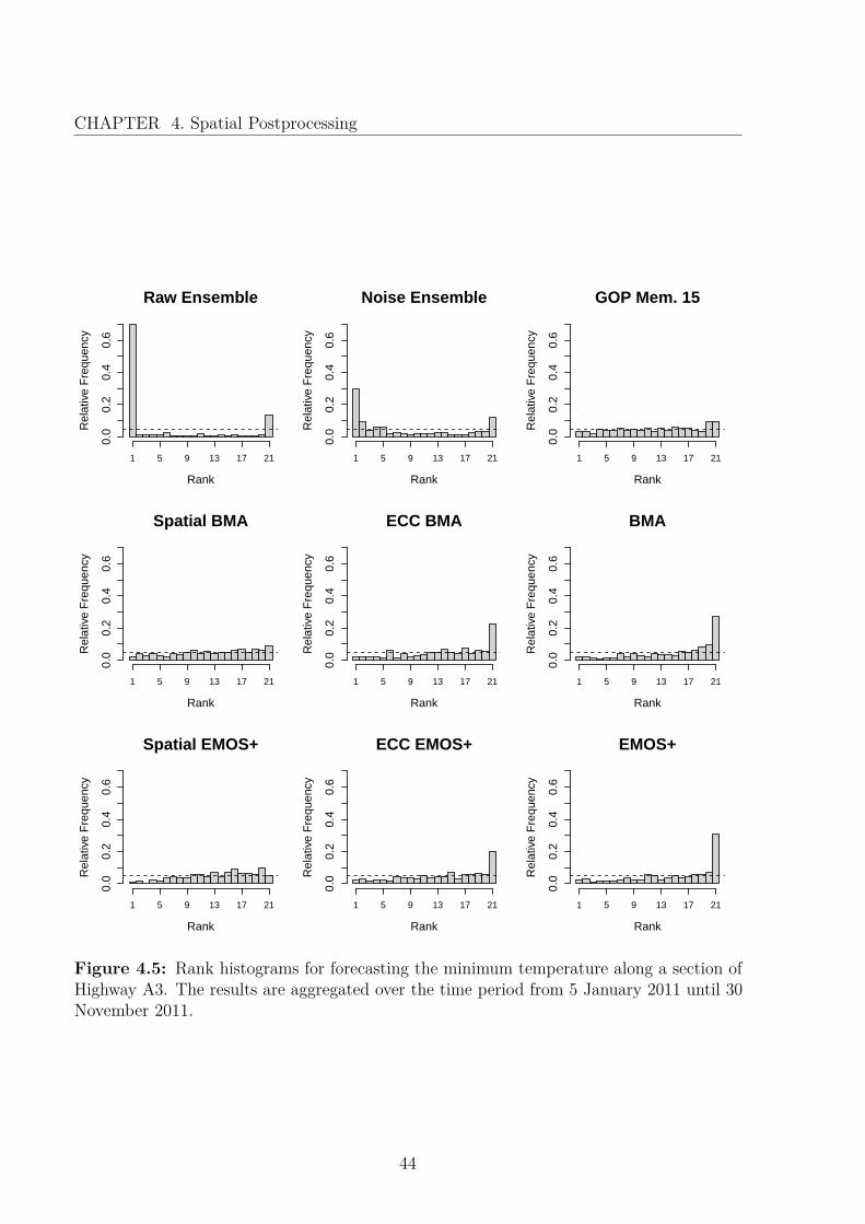
CHAPTER 4. Spatial Postprocessing
Raw Ensemble
Rank
Rel
ativ
e F
requ
ency
0.0
0.2
0.4
0.6
1 5 9 13 17 21
Noise Ensemble
Rank
Rel
ativ
e F
requ
ency
0.0
0.2
0.4
0.6
1 5 9 13 17 21
GOP Mem. 15
Rank
Rel
ativ
e F
requ
ency
0.0
0.2
0.4
0.6
1 5 9 13 17 21
Spatial BMA
Rank
Rel
ativ
e F
requ
ency
0.0
0.2
0.4
0.6
1 5 9 13 17 21
ECC BMA
Rank
Rel
ativ
e F
requ
ency
0.0
0.2
0.4
0.6
1 5 9 13 17 21
BMA
Rank
Rel
ativ
e F
requ
ency
0.0
0.2
0.4
0.6
1 5 9 13 17 21
Spatial EMOS+
Rank
Rel
ativ
e F
requ
ency
0.0
0.2
0.4
0.6
1 5 9 13 17 21
ECC EMOS+
Rank
Rel
ativ
e F
requ
ency
0.0
0.2
0.4
0.6
1 5 9 13 17 21
EMOS+
Rank
Rel
ativ
e F
requ
ency
0.0
0.2
0.4
0.6
1 5 9 13 17 21
Figure 4.5: Rank histograms for forecasting the minimum temperature along a section ofHighway A3. The results are aggregated over the time period from 5 January 2011 until 30November 2011.
44
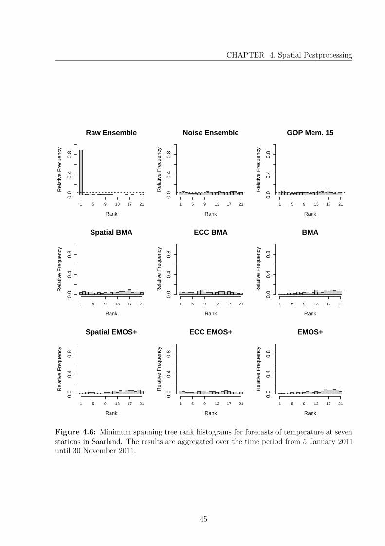
CHAPTER 4. Spatial Postprocessing
Raw Ensemble
Rank
Rel
ativ
e F
requ
ency
0.0
0.4
0.8
1 5 9 13 17 21
Noise Ensemble
Rank
Rel
ativ
e F
requ
ency
0.0
0.4
0.8
1 5 9 13 17 21
GOP Mem. 15
Rank
Rel
ativ
e F
requ
ency
0.0
0.4
0.8
1 5 9 13 17 21
Spatial BMA
Rank
Rel
ativ
e F
requ
ency
0.0
0.4
0.8
1 5 9 13 17 21
ECC BMA
Rank
Rel
ativ
e F
requ
ency
0.0
0.4
0.8
1 5 9 13 17 21
BMA
Rank
Rel
ativ
e F
requ
ency
0.0
0.4
0.8
1 5 9 13 17 21
Spatial EMOS+
Rank
Rel
ativ
e F
requ
ency
0.0
0.4
0.8
1 5 9 13 17 21
ECC EMOS+
Rank
Rel
ativ
e F
requ
ency
0.0
0.4
0.8
1 5 9 13 17 21
EMOS+
Rank
Rel
ativ
e F
requ
ency
0.0
0.4
0.8
1 5 9 13 17 21
Figure 4.6: Minimum spanning tree rank histograms for forecasts of temperature at sevenstations in Saarland. The results are aggregated over the time period from 5 January 2011until 30 November 2011.
45


Chapter 5
Discussion
In this thesis, we have demonstrated the importance of spatial modeling in ensemblepostprocessing. Besides reviewing the existing method spatial BMA (Berrocal et al., 2007),we have introduced a similar approach, based on EMOS+. Both models are obtainedby combining state of the art univariate postprocessing methods with GOP. Thus, thepredictive distributions are based on spatial statistical and ensemble information. Forspatial EMOS+, the predictive density for a weather field is a multivariate normal densitycentered at the bias-corrected ensemble, whereas in the case of BMA the predictive densityis a weighted average over the multivariate Gaussian density of each bias-corrected member.
In a case study with COSMO-DE-EPS, the spatial EMOS+ and spatial BMA outper-formed all other methods including the multivariate ECC approaches. In particular, whenevaluating the composite quantities of minimum and average temperatures, the multivariatemodels showed their superiority.
However, there remain several possibilities for improvements and further investigation.The presented methods, spatial BMA and EMOS+, are only applicable to weather variableswhose distribution of forecast errors can be approximated by a normal distribution. Berrocalet al. (2008) proposed a two-stage spatial model for producing correlated probabilisticforecasts of precipitation accumulation. Further development is needed in order to addressvariables such as wind gust or even wind speed.
Additionally, there are options for advances within spatial BMA and EMOS+. Forboth methods, the bias correction is based on linear least squares regression, which doesnot account for differences in terrain, such as altitude or land use. A more sophisticatedapproach might yield better results.
47
CHAPTER 5. Discussion
Moreover, local parameter estimation such as proposed by Kleiber et al. (2011) couldfurther improve the forecast performance. In particular considering the histogram witha uniform center and two bars at the sides, discussed in Section 3.6, a model with localparameters might resolve this phenomenon. If the forecasts were calibrated locally, thestructure of the error fields would be more realistic and the overall parameter estimationfor the GOP method would yield better results.
In the case of GOP, there are several ways to reduce the computational cost of parameterestimation. We used a rolling training period and estimated the covariance parametersdaily. If the variable of interest is temporal stationary over the years and a larger data setis available, the estimation can be based on a previous year or season. For spatial EMOS+,we only estimated the covariance parameters for the ensemble mean, which performed aswell as spatial BMA, for which the parameters are estimated individually for each member.Hence, in order to speed up computational time for spatial BMA, the member-specificparameter estimation can be replaced as well.
When modeling the covariance structure with the GOP method, we have shown that anexponential correlation function with parameters based on simple variogram estimationyields slightly better results than the modeling with a Mátern correlation function, whoseparameters are obtained by maximum likelihood estimation. However, there might still beroom for improvement with different covariance structures, as discussed in e.g. Gneiting(1999), which represents the atmosphere more accurately.
Obviously, our choice of the length of the training period is subject to debate. However,due to shortage of data, out-of-sample comparison of different lengths was not possible andso we followed the proposal by Berrocal et al. (2007). Given data sets over longer timeperiods, data from the same season of previous years could be included into the trainingperiod (Hamill et al., 2004).
When evaluating the forecasting performance of the multivariate postprocessing methods,we found the improvements over univariate postprocessing to be quite significant in theassessment of forecasts for aggregated quantities. However, they were not visible in themultivariate energy score and Euclidean error. We suspect that these scores are notsufficiently sensitive to slight variations in the multidimensional structure, and thus are nota good verification tool for this task, but further research on this topic is needed.
Motivated by the high correlation of the forecast errors within COSMO-DE-EPS, whichwas neither accounted for by the BMA weights nor the EMOS coefficients, as the valuesvaried drastically over time, we also investigated a ridge regression approach. Whencalculating the predictive mean, we applied linear least squares, but also introduced apenalty term, which should force the coefficients to be similar, if the members were strongly
48

CHAPTER 5. Discussion
correlated. We proposed that two members should be assigned similar coefficients, if theywere based on the same global model or were produced by the same model formulation ofCOSMO-DE-EPS. However, our attempt failed to yield better results than original EMOSor BMA in terms of MAE and consequently this line of research was not pursued anyfurther.
In conclusion, we have demonstrated that spatial EMOS+ and spatial BMA performvery well, despite the fact that there are still many possibilities for improvement or changesin either method. Our verification results for composite quantities have demonstrated onceagain the need for spatial modeling in ensemble postprocessing. Also, we have addressedsome of the issues that arise in the statistical postprocessing of COSMO-DE-EPS and hopethat further research will provide solutions to these.
49

Appendix A
Verification Methods
The goal of probabilistic forecasts is to “maximize sharpness subject to calibration” (Gneitinget al., 2007). Calibration depends on the observations as well as the forecasts, measuringthe statistical consistency between both. This means that a predicted event should onaverage occur as often as its forecast probability indicates. Sharpness is a characteristic ofthe forecast only and measures the concentration of the predictive distribution. Illustratingthe concept, a small standard deviation yields a sharp forecast, whereas a large dispersionaround the distribution’s mean does not reflect a sharp forecast.
There are several techniques to assess the predictive performance of forecasts, consideringsharpness and calibration individually as well as simultaneously. Here, we present a selectionof tools which we have used in the proceeding chapters to evaluate the performance of thecompeting forecasters. On account of the fact that we produce one-dimensional forecasts aswell as forecast fields with up to 514 dimensions, the shown methods not only cover theunivariate, but also the multivariate case. They can be applied to ensemble forecasts aswell as predictive distributions. However, the distinction between both is rather artificial,because by sampling from the predictive distribution, an ensemble is obtained or, on theother hand, an ensemble can be replaced by an appropriate distribution. Thus, both typesof forecasts can be transformed into each another.
Here, we first present tools to check calibration, followed by a method to evaluate thesharpness of forecasts. Then, we introduce proper scoring rules, which address sharpnessand calibration simultaneously. Finally, we present the empirical variogram coverage forforecasting fields.
51
APPENDIX A. Verification Methods
A.1 Assessing Calibration
As mentioned before, calibration is a measure for the statistical consistency between theforecasts and the verifying observations, which means that an event with a certain predictedprobability should on average occur as many times as has been predicted. Depending onthe type of the forecast, there are several ways to assess calibration. Given a probabilisticforecast with a predictive cumulative distribution function (CDF) for a univariate quantity,usually a probability integral transform (PIT) histogram (Dawid, 1984; Diebold et al.,1998) is employed. In case of an ensemble forecast, the corresponding counterpart is theverification rank histogram (VRH) or Talagrand diagram (Anderson, 1996; Hamill andColucci, 1997; Talagrand et al., 1997). A method to assess the calibration of a multivariatequantity is the minimum spanning tree (Smith, 2001; Gneiting et al., 2008).
Probability Integral Transform Histogram
In order to assess the calibration of a univariate forecast distribution F , the PIT histogram(Dawid, 1984; Diebold et al., 1998) is frequently used. Its idea is based on the assumptionthat nature samples the materializing event y from an unknown, true distribution G. Then,for all forecasts and observations available, the PIT values p = F (y) are determined andcollected. For F to equal G and therefore an ideal forecaster, it is a necessary conditionthat these values have a uniform distribution on [0, 1] (Gneiting et al., 2007).
In practice, for every forecast the PIT value is computed, collected and afterwards sortedinto bins in order to plot a histogram. When interpreting the outcome of the histogram,we take a look at its shape. If the histogram shows uniformity, it indicates calibration. AU-shape reveals that the predictive distributions are underdispersive, meaning that theyare too narrow. On the other hand, a hump-shaped histogram suggests that too manyobservations lie in the center of the distributions and therefore the prediction intervals aretoo wide, resulting in overdispersion. If the histograms resemble a triangle, the predictivedistributions are biased.
Rank Histogram
Considering a discrete ensemble forecast, the VRH or Talagrand diagram (Anderson,1996; Hamill and Colucci, 1997; Talagrand et al., 1997) replaces the PIT histogram. Theinterpretation of the resulting histogram stays the same, but the construction differs. Givenan ensemble of size M , for each forecast available, the rank of the observation y in the set
52

APPENDIX A. Verification Methods
of all forecasts x1, ..., xM , combined with y, is determined. Afterwards, a histogram of allaggregated ranks, which range from 1 to m+ 1, is plotted.
Minimum Spanning Tree Rank Histogram
In order to check the calibration of multivariate ensemble forecasts, the minimum spanningtree (MST) rank histogram (Smith, 2001) is an appropriate tool. Evaluating an ensembleforecast {xi∈ Rd|i = 1, ...,M}, d ∈ N, with the observation x0 ∈ Rd, the construction ofthe MST histogram follows these steps:
1. Standardize
Sometimes, it can be useful to apply a principal component transform to the set offorecasts and observations {xi ∈ Rd|i = 0, ...,M}, in order to generate standardizedquantities {x?i ∈ Rd|i = 0, ...,M}.
2. Compute minimum spanning tree
Considering every subset {x?i ∈ Rd|i ∈ {0, ...,M} \ j}, for j = 0, ...M , where eitherthe observation or one of the ensemble members has been removed, determine theminimum spanning tree and calculate its length, lj > 0.
3. MST rank
The MST rank r equals the rank of l0 in the pool of all lengths li, i = 0, ...,M . If tiesoccur, they are resolved at random. Let
s< =M∑i=0
I(li < l0)
be the number of MST lengths that are smaller than the length of the MST withoutthe observation, and
s= =M∑i=0
I(li = l0)
the number of MST lengths which equal the length of the MST without the observation.Then the MST rank r is chosen from a discrete uniform distribution on the set{s< + 1, ..., s< + s=}, so that r ∈ {1, ...,M + 1}.
53
APPENDIX A. Verification Methods
4. Aggregate ranks and plot histogram
Finally, we collect all MST ranks over all dates and locations available and plot thecorresponding histogram.
For the calculation of the minimum spanning trees, we employ the R package vegan byOksanen et al. (2011).
The interpretation of this tool differs from that of other histogram-based methods. Anunderdispersed or biased ensemble results in many low MST ranks. In contrast, if theensemble is overdispersed, the higher ranks are overpopulated. Given an ideal forecaster, sothat the ensemble members and the observation can be considered exchangeable, the MSTrank histogram appears uniform.
A.2 Assessing Sharpness
Sharpness measures the concentration of the predictive distribution and is therefore afeature of the forecast only. Following the principle of “maximizing sharpness subject tocalibration” (Gneiting et al., 2007), the more concentrated the distribution, the sharper it is,the better we rate it, subject to calibration. When evaluating the sharpness, we determinethe width of the prediction intervals. To facilitate comparability of the postprocessedforecasts with the M member ensemble, often the nominal M−1
M+1 · 100% prediction intervalis used, because its coverage corresponds to that of the ensemble range.
A.3 Proper Scoring Rules
A very important tool to assess a forecaster’s performance are proper scoring rules, whichevaluate sharpness and calibration concurrently. Scores are negatively oriented and canbe interpreted as a penalty, which the forecaster wants to reduce. They are based on thepredictive distribution F and the verifying observation y. If we assume y to be drawn froma true, but unknown distribution G, the expected value is written as s(F,G). We call ascoring rule proper if it is minimized for F = G; it is strictly proper if s(F,G) > s(G,G)for all F 6= G. The theory of strictly proper scoring rules is discussed further in Gneitingand Raftery (2007).
Here, we present the equations for each score independently of time and space. Inpractice, we calculate the scores for all times and locations available and then determinethe average score
54

APPENDIX A. Verification Methods
s = 1n
n∑i=1
s(Fi, yi),
where n denotes the number of available forecasts.
Brier Score
The Brier score (BS), also referred to as quadratic score, is a well-known scoring rule forunivariate quantities with a CDF, which was first presented by Brier (1950), and is definedas
bs(z) = (F (z)− I(z ≥ y))2 ,
where z ∈ R is a threshold value, F represents the predictive distribution and y the verifyingobservation.
Continuous Rank Probability Score
The continuous rank probability score (CRPS), also applicable to univarite quantities,corresponds to the integral of the BS over all threshold values z ∈ R (Toth and Kalnay,1997). It was proposed by Matheson and Winkler (1976) and further developed in Hersbach(2000), Gneiting et al. (2005) and Wilks (2006):
crps(F, y) =ˆ ∞−∞
(F (z))− I(z ≥ y))2dz = EF |X − y| −12EP |X −X
′|,
where F is the predictive distribution, y represents the verifying observation, and X andX ′ are independent random variables with distribution function F and finite first moment.Gneiting and Raftery (2007) showed the second equality.
Energy Score
A multivariate generalization of the CRPS is the energy score (ES), described in Gneitingand Raftery (2007), which is defined as
es(F,y) = EF ||X− y|| − 12EF ||X−X′||,
55

APPENDIX A. Verification Methods
where || · || is the Euclidean norm, F represents the predictive distribution, y ∈ Rd is theobservation and X∈ Rd and X′∈ Rd are independent random vectors with distribution F .For d = 1, the energy score reduces to the CRPS. In order to facilitate computability, wereplace the ES for normal or related predictive densities with a Monte Carlo approximation.In this case, we draw a sample x1, ...,xk ∈ Rd of size k = 10, 000 from the predictivedistribution F and estimate the ES via
es(F,y) = 1k
k∑i=1||xi − y|| − 1
2(k − 1)
k−1∑i=1||xi − xi+1||.
We follow the same technique when calculating the CRPS. Given a forecast ensemble,instead of a predictive distribution, the ES can be calculated, using
es(Fens,y) = 1M
M∑i=1||xi − y|| − 1
2M2
M∑i=1
M∑j=1||xi − xj||,
where point masses 1M
are placed on each ensemble member x1, ...,xM ∈ Rd.
Mean Absolute Error
In the case of a deterministic forecast, the CRPS can be reduced to the absolute error(Gneiting et al., 2005):
ae(µ, y) = |µ− y|,
with µ being the median of F .
Euclidean Error
The multivariate generalization of the absolute error is the Euclidean error
ee(F,y) = ||smedF − y||,
where smedF defines the spatial median of the predictive distribution F , which can bedefined as (Gneiting, 2011; Vardi and Zhang, 2000)
56
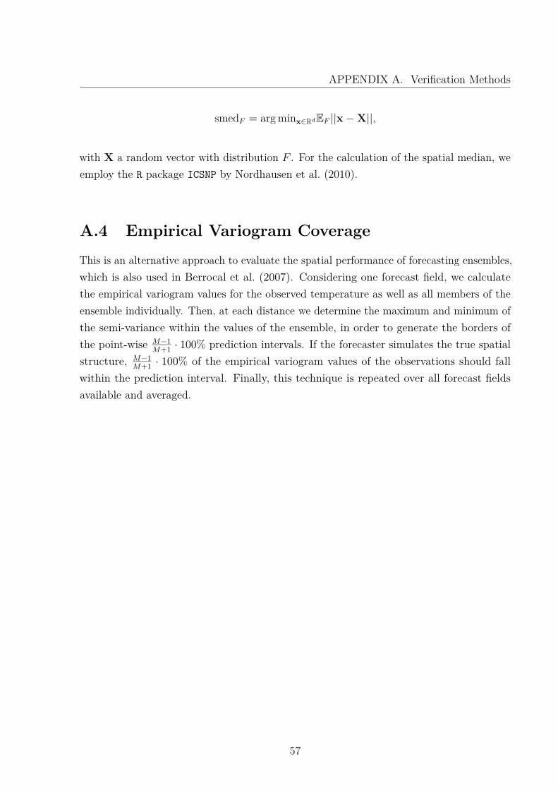
APPENDIX A. Verification Methods
smedF = arg minx∈RdEF ||x−X||,
with X a random vector with distribution F . For the calculation of the spatial median, weemploy the R package ICSNP by Nordhausen et al. (2010).
A.4 Empirical Variogram Coverage
This is an alternative approach to evaluate the spatial performance of forecasting ensembles,which is also used in Berrocal et al. (2007). Considering one forecast field, we calculatethe empirical variogram values for the observed temperature as well as all members of theensemble individually. Then, at each distance we determine the maximum and minimum ofthe semi-variance within the values of the ensemble, in order to generate the borders ofthe point-wise M−1
M+1 · 100% prediction intervals. If the forecaster simulates the true spatialstructure, M−1
M+1 · 100% of the empirical variogram values of the observations should fallwithin the prediction interval. Finally, this technique is repeated over all forecast fieldsavailable and averaged.
57
Appendix B
Plots of the Empirical Variograms
In R, there are several packages provided for calculating empirical variograms. Berrocalet al. (2007) suggest the use of the package ProbForecastGOP (Berrocal et al., 2010). Wealso compute variograms based on the package RandomFields by Schlather (2011). AsFigure B.1 shows, the results for the same member differ substantially on certain days,depending on the package. Since models based on RandomFields yield better forecastingresults, we use this package for the entire thesis.
58
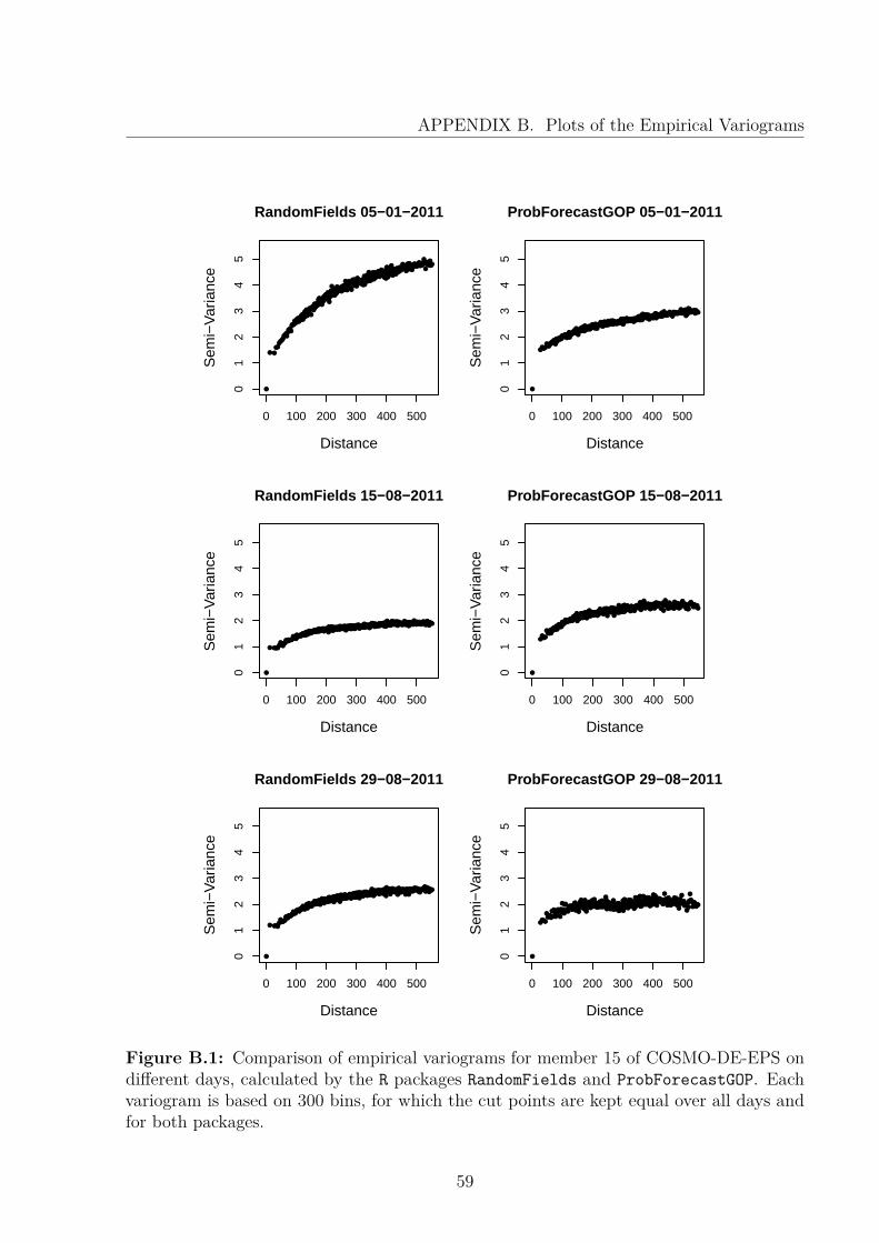
APPENDIX B. Plots of the Empirical Variograms
●
● ●●●
●●●●●●●●
●●●●●
●●●●●●●●●●●●●●●●●●●●●●●●●●●●●●●●●
●●●●●●●●●●●●●●●●●●●●●●
●●●●●●●●●●●●●●●●●●
●●●●●●
●●●●●●●●
●●●●
●●●●●●●●●●●●●●●●●●●●●
●●●●●
●●●●●●●●●●●
●●●●●●●●●●●●
●●●●●●●●●●●
●●●●●●●●●
●●●●●●●●
●●●●●●●●●●●●●●●●●●●●●●●●●●●●●●●●●●●●●●●
●●
●
●●●●●●●●●●
●●●●●●●●●●●●●●●
●●●●●●●●●●●●●
●●●●●●●●●
●●●●●●●●●
●●●●●
●●●
●●●●●
●●●
0 100 200 300 400 500
01
23
45
RandomFields 05−01−2011
Distance
Sem
i−V
aria
nce
●
●●●●
●●●●●●●
●●●●●●●●●●●
●●●●●●●●●●●●●●●●●●●
●●●●●●●●●●●●●●●●●●●●●●●●●●●●●●●
●●●●●●●●●●●●●●●●●●●●●●●●●●●●●
●●●●●●●●●●●●●●●●
●●●●●●●●●●●●●●●●●●●●●●●●●●●●●
●●●●●●●●●●●●●●●●●●●●
●●●●●●●●●●●●●●●●●●
●●●●●●●●●●●●●●●●●●●●●●●●●●●●
●●●●●●●●●●●●●●●●●●
●●●●●●●●●●●●●●●
●●●●●●●●●●●●●●
●●●●●●●●●●●●●●●●●●
●●●●●●●
●●●●●●●●●●●●
●●●
0 100 200 300 400 500
01
23
45
ProbForecastGOP 05−01−2011
Distance
Sem
i−V
aria
nce
●
● ●●●●●●●
●●●●●●●●●●
●●●●●●
●●●●●●●●●●●●●●●
●●●●●●●●●●●●●●●●
●●●●●●●●●●●●●●●●●●●
●●●●●●●●●●●●●●
●●●●●●●●●●●●●●●●●●●●●●●●●●
●●●●●●●●●●●●
●●●●●●●●●●●●●●●●●●●
●●●●●●●●●●●●●●●●●●●●●●●●●
●●●●●●●●●●●●●●●●●●●●●●
●●●●●●●●●●●●●●●●●●●●
●●●●●●●●●●●●●●●●●●●●●●●●●
●●●●●●●●●●●●●
●●●●●●●●●●●●●●●●●●●●●●●●●●
●●●●●●●●●●●●
●●●●●●●●
●●●
0 100 200 300 400 500
01
23
45
RandomFields 15−08−2011
Distance
Sem
i−V
aria
nce
●
●●●●
●●●●●●●●●●●●●●●●
●●●●●●●
●●●●●●●●●●●●●●
●●●●●●●
●●●●●●●●●●●●●●●●●●●●●●●●●●●●●●●●●●●●●●●●●●●
●●●●●●●●●●●●●●●●●●
●●●●●●●●●
●●●●●●●●●●●●●●●●
●●●●●●●●●●●●●
●●●●●●●●●●●●●
●●●●●●●●●●●●●●●●●●●●●●●●●●
●●●●●●●●●●●●●●
●●●●●●●●●●●●●●●●●●●●●
●●●●●●●●●●●●●●●●●●
●●●●●●●●●
●●●●●●●●●●●●●●●●●●
●
●●●●●●●●●●●●●●●●●
●●●●●●●●●●●●●●●
0 100 200 300 400 500
01
23
45
ProbForecastGOP 15−08−2011
Distance
Sem
i−V
aria
nce
●
● ●●●●●●●●●
●●●●●●●●●
●●●●●●●●●●●
●●●●●●●●●
●●●●●●●●●●●●●●
●●●●●●●●●●●●●●●●●●●●●●●●
●●●●●●●●●●●●●●●●●●
●●●●●●●●●●●●●
●●●●●●●●●●●●●●●●●●●●●●●●
●●●●●●●●●●●●●●●●●●●●●●●●●●●●●●●●●●●●●●●●●●●
●●●●●●●●●●●●●●●●●●●●●●●●●●●●●●●●●●●●●
●●●●●●●●●●●●●●●
●●●●●●●●●●●●●●●●●●●●
●●●●●●●●●●●
●●●●●●●●●●●●●●●●●●
●●●●●●●●●●●●●●●●●●●●●●●
0 100 200 300 400 500
01
23
45
RandomFields 29−08−2011
Distance
Sem
i−V
aria
nce
●
●●●●
●●●●●
●●
●●●●●●●●●
●●
●
●●●
●●
●●●●●●●●●●
●●●●●●●
●●●●●●●
●●●●●●●●●●●●
●●●●
●●●●●●●●●●●●●●●●●
●
●●●●●●●●●●●●●●●●●●●
●●●●●●●●
●●
●●
●●●●●●●●●●●●●●●●
●
●●●●●●●●●●●●
●●●●●●●●●●●
●●
●●
●●●●●●●●●●●●●●●●●●●●●●●●
●●
●
●●
●●●●●●●●●
●●●●●●●●●●●●●●●●●●●●●
●●●●●●●●●
●●
●●●●●●●●●●●●●●●●●●●
●
●●●●
●●●●●●●●●●●●●●●●
●●●●●●●
●
●●●●●●
●
●●
●
●
●●●●●●●●●
0 100 200 300 400 500
01
23
45
ProbForecastGOP 29−08−2011
Distance
Sem
i−V
aria
nce
Figure B.1: Comparison of empirical variograms for member 15 of COSMO-DE-EPS ondifferent days, calculated by the R packages RandomFields and ProbForecastGOP. Eachvariogram is based on 300 bins, for which the cut points are kept equal over all days andfor both packages.
59

Appendix C
Further Verification Results
In addition to the results presented in Subsection 4.5.2, we also consider multivariateassessment of different subsets of the data, another aggregated variable, and the univariateperformance of the forecasts. The interpretation of these results does not differ from thediscussion in 4.5.2. However, for the sake of completeness, we add our findings.
Table C.1 presents the scores for the prediction of the average temperature in everyGerman state individually; the results are then averaged over all states. Figure C.1exemplary shows the rank histograms for Hessen.
Furthermore, we consider two subsets of the data. One contains the observation sitesat the airports in Hamburg, Berlin and Frankfurt, separated by a great distance, and theother consists of three closely located stations in Berlin. The corresponding scores can beseen in the Tables C.2 and C.3, as well as the minimum spanning tree rank histograms inthe Figures C.2 and C.3.
For forecasts at individual sites, spatial BMA or ECC BMA are equal to the originalBMA. Thus, the one-dimensional assessment of the spatial techniques coincides with theirunivariate counterparts, as can be seen in Table C.4 and Figure C.4. The slight differencesare due to variability in drawing the forecast samples. Theoretically, the same applies toEMOS+. However, we found that for spatial EMOS+ the predicted site-specific variance isgreater than for regular EMOS+. The reason for this might be rooted in the normalizationprocess of the error field.
60
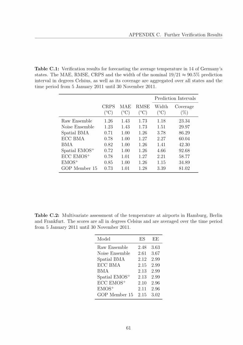
APPENDIX C. Further Verification Results
Table C.1: Verification results for forecasting the average temperature in 14 of Germany’sstates. The MAE, RMSE, CRPS and the width of the nominal 19/21 ≈ 90.5% predictioninterval in degrees Celsius, as well as its coverage are aggregated over all states and thetime period from 5 January 2011 until 30 November 2011.
Prediction IntervalsCRPS MAE RMSE Width Coverage(°C) (°C) (°C) (°C) (%)
Raw Ensemble 1.26 1.43 1.73 1.18 23.34Noise Ensemble 1.23 1.43 1.73 1.51 29.97Spatial BMA 0.71 1.00 1.26 3.78 86.29ECC BMA 0.78 1.00 1.27 2.27 60.04BMA 0.82 1.00 1.26 1.41 42.30Spatial EMOS+ 0.72 1.00 1.26 4.66 92.68ECC EMOS+ 0.78 1.01 1.27 2.21 58.77EMOS+ 0.85 1.00 1.26 1.15 34.89GOP Member 15 0.73 1.01 1.28 3.39 81.02
Table C.2: Multivariate assessment of the temperature at airports in Hamburg, Berlinand Frankfurt. The scores are all in degrees Celsius and are averaged over the time periodfrom 5 January 2011 until 30 November 2011.
Model ES EERaw Ensemble 2.48 3.63Noise Ensemble 2.61 3.67Spatial BMA 2.12 2.99ECC BMA 2.15 2.99BMA 2.13 2.99Spatial EMOS+ 2.13 2.99ECC EMOS+ 2.10 2.96EMOS+ 2.11 2.96GOP Member 15 2.15 3.02
61
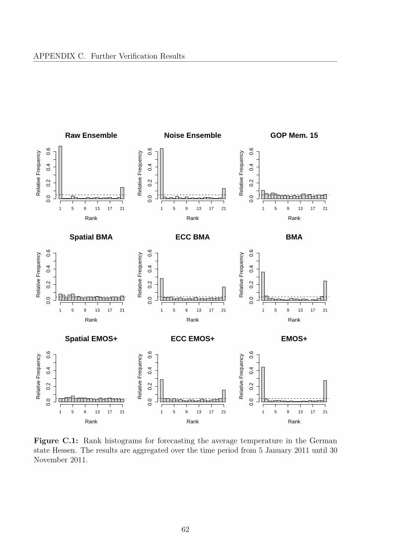
APPENDIX C. Further Verification Results
Raw Ensemble
Rank
Rel
ativ
e F
requ
ency
0.0
0.2
0.4
0.6
1 5 9 13 17 21
Noise Ensemble
Rank
Rel
ativ
e F
requ
ency
0.0
0.2
0.4
0.6
1 5 9 13 17 21
GOP Mem. 15
Rank
Rel
ativ
e F
requ
ency
0.0
0.2
0.4
0.6
1 5 9 13 17 21
Spatial BMA
Rank
Rel
ativ
e F
requ
ency
0.0
0.2
0.4
0.6
1 5 9 13 17 21
ECC BMA
Rank
Rel
ativ
e F
requ
ency
0.0
0.2
0.4
0.6
1 5 9 13 17 21
BMA
Rank
Rel
ativ
e F
requ
ency
0.0
0.2
0.4
0.6
1 5 9 13 17 21
Spatial EMOS+
Rank
Rel
ativ
e F
requ
ency
0.0
0.2
0.4
0.6
1 5 9 13 17 21
ECC EMOS+
Rank
Rel
ativ
e F
requ
ency
0.0
0.2
0.4
0.6
1 5 9 13 17 21
EMOS+
Rank
Rel
ativ
e F
requ
ency
0.0
0.2
0.4
0.6
1 5 9 13 17 21
Figure C.1: Rank histograms for forecasting the average temperature in the Germanstate Hessen. The results are aggregated over the time period from 5 January 2011 until 30November 2011.
62
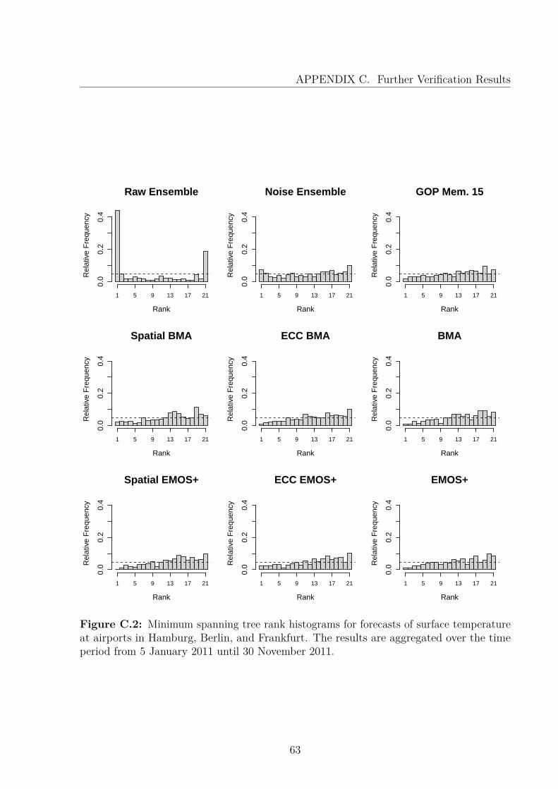
APPENDIX C. Further Verification Results
Raw Ensemble
Rank
Rel
ativ
e F
requ
ency
0.0
0.2
0.4
1 5 9 13 17 21
Noise Ensemble
Rank
Rel
ativ
e F
requ
ency
0.0
0.2
0.4
1 5 9 13 17 21
GOP Mem. 15
Rank
Rel
ativ
e F
requ
ency
0.0
0.2
0.4
1 5 9 13 17 21
Spatial BMA
Rank
Rel
ativ
e F
requ
ency
0.0
0.2
0.4
1 5 9 13 17 21
ECC BMA
Rank
Rel
ativ
e F
requ
ency
0.0
0.2
0.4
1 5 9 13 17 21
BMA
Rank
Rel
ativ
e F
requ
ency
0.0
0.2
0.4
1 5 9 13 17 21
Spatial EMOS+
Rank
Rel
ativ
e F
requ
ency
0.0
0.2
0.4
1 5 9 13 17 21
ECC EMOS+
Rank
Rel
ativ
e F
requ
ency
0.0
0.2
0.4
1 5 9 13 17 21
EMOS+
Rank
Rel
ativ
e F
requ
ency
0.0
0.2
0.4
1 5 9 13 17 21
Figure C.2: Minimum spanning tree rank histograms for forecasts of surface temperatureat airports in Hamburg, Berlin, and Frankfurt. The results are aggregated over the timeperiod from 5 January 2011 until 30 November 2011.
63
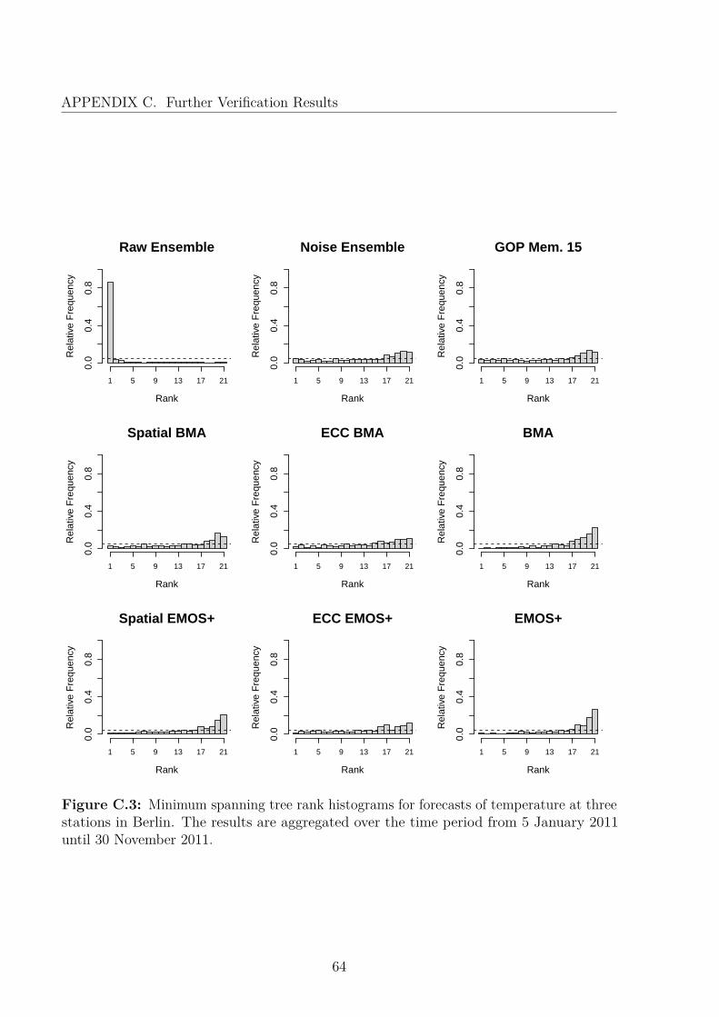
APPENDIX C. Further Verification Results
Raw Ensemble
Rank
Rel
ativ
e F
requ
ency
0.0
0.4
0.8
1 5 9 13 17 21
Noise Ensemble
Rank
Rel
ativ
e F
requ
ency
0.0
0.4
0.8
1 5 9 13 17 21
GOP Mem. 15
Rank
Rel
ativ
e F
requ
ency
0.0
0.4
0.8
1 5 9 13 17 21
Spatial BMA
Rank
Rel
ativ
e F
requ
ency
0.0
0.4
0.8
1 5 9 13 17 21
ECC BMA
Rank
Rel
ativ
e F
requ
ency
0.0
0.4
0.8
1 5 9 13 17 21
BMA
Rank
Rel
ativ
e F
requ
ency
0.0
0.4
0.8
1 5 9 13 17 21
Spatial EMOS+
Rank
Rel
ativ
e F
requ
ency
0.0
0.4
0.8
1 5 9 13 17 21
ECC EMOS+
Rank
Rel
ativ
e F
requ
ency
0.0
0.4
0.8
1 5 9 13 17 21
EMOS+
Rank
Rel
ativ
e F
requ
ency
0.0
0.4
0.8
1 5 9 13 17 21
Figure C.3: Minimum spanning tree rank histograms for forecasts of temperature at threestations in Berlin. The results are aggregated over the time period from 5 January 2011until 30 November 2011.
64
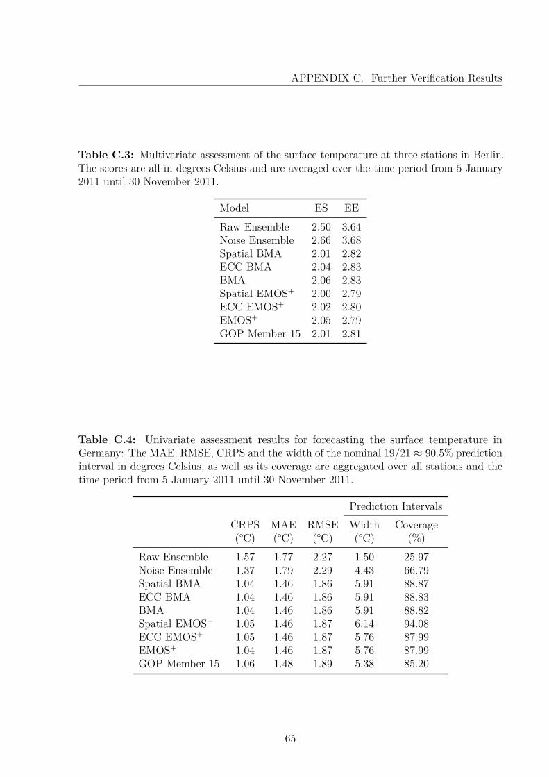
APPENDIX C. Further Verification Results
Table C.3: Multivariate assessment of the surface temperature at three stations in Berlin.The scores are all in degrees Celsius and are averaged over the time period from 5 January2011 until 30 November 2011.
Model ES EERaw Ensemble 2.50 3.64Noise Ensemble 2.66 3.68Spatial BMA 2.01 2.82ECC BMA 2.04 2.83BMA 2.06 2.83Spatial EMOS+ 2.00 2.79ECC EMOS+ 2.02 2.80EMOS+ 2.05 2.79GOP Member 15 2.01 2.81
Table C.4: Univariate assessment results for forecasting the surface temperature inGermany: The MAE, RMSE, CRPS and the width of the nominal 19/21 ≈ 90.5% predictioninterval in degrees Celsius, as well as its coverage are aggregated over all stations and thetime period from 5 January 2011 until 30 November 2011.
Prediction IntervalsCRPS MAE RMSE Width Coverage(°C) (°C) (°C) (°C) (%)
Raw Ensemble 1.57 1.77 2.27 1.50 25.97Noise Ensemble 1.37 1.79 2.29 4.43 66.79Spatial BMA 1.04 1.46 1.86 5.91 88.87ECC BMA 1.04 1.46 1.86 5.91 88.83BMA 1.04 1.46 1.86 5.91 88.82Spatial EMOS+ 1.05 1.46 1.87 6.14 94.08ECC EMOS+ 1.05 1.46 1.87 5.76 87.99EMOS+ 1.04 1.46 1.87 5.76 87.99GOP Member 15 1.06 1.48 1.89 5.38 85.20
65
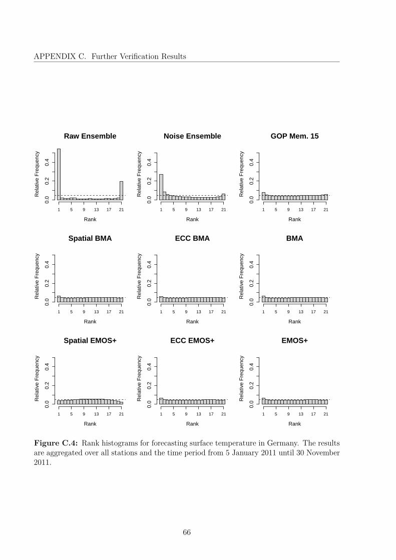
APPENDIX C. Further Verification Results
Raw Ensemble
Rank
Rel
ativ
e F
requ
ency
0.0
0.2
0.4
1 5 9 13 17 21
Noise Ensemble
Rank
Rel
ativ
e F
requ
ency
0.0
0.2
0.4
1 5 9 13 17 21
GOP Mem. 15
Rank
Rel
ativ
e F
requ
ency
0.0
0.2
0.4
1 5 9 13 17 21
Spatial BMA
Rank
Rel
ativ
e F
requ
ency
0.0
0.2
0.4
1 5 9 13 17 21
ECC BMA
Rank
Rel
ativ
e F
requ
ency
0.0
0.2
0.4
1 5 9 13 17 21
BMA
Rank
Rel
ativ
e F
requ
ency
0.0
0.2
0.4
1 5 9 13 17 21
Spatial EMOS+
Rank
Rel
ativ
e F
requ
ency
0.0
0.2
0.4
1 5 9 13 17 21
ECC EMOS+
Rank
Rel
ativ
e F
requ
ency
0.0
0.2
0.4
1 5 9 13 17 21
EMOS+
Rank
Rel
ativ
e F
requ
ency
0.0
0.2
0.4
1 5 9 13 17 21
Figure C.4: Rank histograms for forecasting surface temperature in Germany. The resultsare aggregated over all stations and the time period from 5 January 2011 until 30 November2011.
66
Bibliography
Anderson, J. L. (1996) A Method for Producing and Evaluating Probabilistic Forecastsfrom Ensemble Model Integrations. Journal of Climate, 9, 1518–1530.
Baldauf, M., A. Seifert, J. Förstner, D. Majewski, M. Raschendorfer and T. Reinhardt(2011) Operational Convective-Scale Numerical Weather Prediction with the COSMOModel: Description and Sensitivities. Monthly Weather Review, 139, 3887–3905.
Bao, L., T. Gneiting, E. P. Grimit, P. Guttorp and A. E. Raftery (2010) Bias Correction andBayesian Model Averaging for Ensemble Forecasts of Surface Wind Direction. MonthlyWeather Review, 138, 1811–1821.
Berrocal, V. J., Y. Gel, A. E. Raftery and T. Gneiting (2010) ProbForecastGOP: Prob-abilistic weather forecast using the GOP method. URL http://cran.r-project.org/package=ProbForecastGOP.
Berrocal, V. J., A. E. Raftery and T. Gneiting (2007) Combining Spatial Statistical andEnsemble Information in Probabilistic Weather Forecasts. Monthly Weather Review, 135,1386–1402.
Berrocal, V. J., A. E. Raftery and T. Gneiting (2008) Probabilistic Quantitative PrecipitationField Forecasting using a Two-Stage Spatial Model. The Annals of Applied Statistics, 2,1170–1193.
Bishop, C. M. (2006) Pattern Recognition and Machine Learning. Springer.
Brier, G. W. (1950) Verification of Forecasts Expressed in Terms of Probability. MonthlyWeather Review, 78, 1–3.
Bryd, R. H., P. Lu, J. Nocedal and C. Zhu (1995) A Limited Memory Algorithm for BoundConstrained Optimization. SIAM Journal on Scientific Computing, 16, 1190–1208.
67
BIBLIOGRAPHY
Buizza, R. (1997) Potential Forecast Skill of Ensemble Prediction and Spread and SkillDistributions of the ECMWF Ensemble Prediction System. Monthly Weather Review,125, 99–119.
Cressie, N. A. C. (1985) Fitting Variogram Models by Weighted Least Squares. MathematicalGeology, 17, 563–586.
Dawid, A. P. (1984) Statistical theory: The Prequential Approach (with Discussion andRejoinder). Journal of the Royal Statistical Society Series A, 147, 278–292.
Diebold, F. X., T. A. Gunther and A. S. Tay (1998) Evaluating Density Forecasts withApplications to Financial Risk Management. International Economic Review, 39, 863–883.
Diggle, P. J. and P. J. Ribeiro Jr. (2007) Model-based Geostatistics. Springer.
Eckel, F. A. and F. M. Clifford (2005) Aspects of Effective Mesoscale, Short-Range EnsembleForecasting. Weather and Forecasting, 20, 328–350.
Environmental Modeling Center (2003) The GFS Atmospheric Model. NCEP Off. Note442, Natl. Cent. for Environ. Protection, Camp Spring.
Fraley, C., A. E. Raftery, J. M. Sloughter, T. Gneiting and U. of Washington (2011)ensembleBMA: Probabilistic Forecasting using Ensembles and Bayesian Model Averaging.URL http://cran.r-project.org/package=ensembleBMA.
Gebhardt, C., S. E. Theis, M. Paulat and Z. Ben-Bouallègue (2011) Uncertainties inCOSMO-DE Precipitation Forecasts Introduced by Model Perturbations and Variationof Lateral Boundaries. Atmospheric Research, 100, 168–177.
Gel, Y., A. E. Raftery and T. Gneiting (2004) Calibrated Probabilistic Mesoscale WeatherField Forecasting: The Geostatistical Output Perturbation Method. Journal of theAmerican Statistical Association, 99, 575–583.
Gneiting, T. (1999) Correlation Functions for Atmospheric Data Analysis. Quarterly Journalof the Royal Meteorological Society, 125, 2449–2464.
Gneiting, T. (2011) Making and Evaluating Point Forecasts. Journal of the AmericanStatistical Association, 106, 746–762.
Gneiting, T., F. Balabdaoui and A. E. Raftery (2007) Probabilistic Forecasts, Calibrationand Sharpness. Royal Statistical Society, 69, 243–268.
68
BIBLIOGRAPHY
Gneiting, T., A. E. Raftery, A. H. Westveld and T. Goldman (2005) Calibrated ProbabilisticForecasting Using Ensemble Model Output Statistics and Minimum CRPS Estimation.Monthly Weather Review, 133, 1098–1118.
Gneiting, T., L. I. Stanberry, E. P. Grimit, L. Held and N. A. Johnson (2008) AssessingProbabilistic Forecasts of Multivariate Quantities, with an Application to EnsemblePredictions of Surface Winds. Test, 17, 211–235.
Gneiting, T. G. and A. E. Raftery (2007) Strictly Proper Scoring Rules, Prediction, andEstimation. Journal of the American Statistical Association, 102, 359–378.
Gosset, W. S. (1908) The Probable Error of a Mean. Biometrika, 6, 1–25.
Hamill, T. M. and S. J. Colucci (1997) Verification of Eta-RSM Short-Range EnsembleForecasts. Monthly Weather Review, 125, 1312–1327.
Hamill, T. M., J. S. Whitaker and X. Wei (2004) Ensemble Reforecasting: ImprovingMedium-Range Forecast Skill Using Retrospective Forecasts. Monthly Weather Review,132, 1434–1447.
Hersbach, H. (2000) Decomposition of the Continuous Ranked Probability Score for Ensem-ble Prediction Systems. Weather and Forecasting, 15, 559–570.
Hoeting, J. A., D. Madigan, A. E. Raftery and C. T. Volinsky (1999) Bayesian ModelAveraging: A Tutorial. Statistical Science, 14, 382–417.
Janssen, P. and J. Bidlot (2002) ECMWF Wave Model (CY25R1). IFS DocumentationCycle CY25r1, Report, ECMWF, Reading, U.K.
Kleiber, W., A. E. Raftery, J. Baars, T. Gneiting, C. F. Mass and E. Grimit (2011) LocallyCalibrated Probabilistic Temperature Forecasting Using Geostatistical Model Averagingand Local Bayesian Model Averaging. Monthly Weather Review, 139, 2630–2649.
Leith, C. E. (1974) Theoretical Skill of Monte-Carlo Forecasts. Monthly Weather Review,104, 409–418.
Leutbecher, M. and T. N. Palmer (2008) Ensemble Forecasting. Journal of ComputationalPhysics, 227, 3515–3539.
Lewis, J. M. (2005) Roots of Ensemble Forecasting. Monthly Weather Review, 133, 1865–1885.
69
BIBLIOGRAPHY
Majewski, D., D. Liermann, P. Prohl, B. Ritter, M. Buchhod, T. Hanisch, P. Gerhard andW. Wergen (2002) The Operational Global Icoshedral-Hexagonal Gridpoint Model GME:Description and High-Resolution Tests. Monthly Weather Review, 130, 319–338.
Matérn, B. (1986) Spatial variation. Springer.
Matheson, J. E. and R. L. Winkler (1976) Scoring Rules for Continuous ProbabilityDistributions. Management Science, 22, 1087–1096.
Nordhausen, K., S. Sirkia, H. Oja and D. E. Tyler (2010) ICSNP: Tools for MultivariateNonparametrics. URL http://cran.r-project.org/package=ICSNP.
Oksanen, J., F. G. Blanchet, R. Kindt, P. Legendre, P. R. Minchin, R. B. O’Hara, G. L.Simpson, P. Solymos, M. H. H. Stevens and H. Wagner (2011) vegan: Community EcologyPackage. URL http://cran.r-project.org/package=vegan.
Peralta, C., Z. Ben Bouallègue, S. E. Theis, C. Gebhardt and M. Buchhold (2012) Accountingfor Initial Condition Uncertainties in COSMO-DE-EPS. Journal of Geophysical Research,117, D07108.
Peralta, C. and M. Buchhold (2011) Initial Condition Perturbations for the COSMO-DE-EPS. COSMO Newsletter, 11, 115–123.
Raftery, A. E., T. Gneiting, F. Balabdaoui and M. Polakowski (2005) Using Bayesian ModelAveraging to Calibrate Forecast Ensembles. Monthly Weather Review, 133, 1155–1174.
Schefzik, R. (2011) Ensemble Copula Coupling. Diploma thesis, Faculty of Mathematicsand Computer Science, Heidelberg University.
Schlather, M. (2011) RandomFields: Simulation and Analysis of Random Fields. URLhttp://cran.r-project.org/package=RandomFields.
Schuhen, N., T. L. Thorarinsdottir and T. Gneiting (2012) Ensemble Model OutputStatistics for Wind Vectors. to appear in Monthly Weather Review.
Sloughter, J. M., T. Gneiting and A. E. Raftery (2010) Probabilistic Wind Speed ForecastingUsing Ensembles and Bayesian Model Averaging. Journal of the American StatisticalAssociation, 105, 25–35.
Sloughter, J. M. L., A. E. Raftery, T. Gneiting and C. Fraley (2007) Probabilistic Quan-titative Precipitation Forecasting Using Bayesian Model Averaging. Monthly WeatherReview, 135, 3209–3220.
70
BIBLIOGRAPHY
Smith, L. A. (2001) Disentangling Uncertainty and Error: on the Predictability of NonlinearSystems. In: A. Mess (ed) Nonlinear dynamics and statistics, 31–64, Birkhäuser, Boston.
Steppeler, J., G. Doms, U. Schättler, H. W. Bitzer, A. Gassmann, U. Damrath andG. Gregoric (2003) Meso-Gamma Scale Forecasts using the Nonhydrostatic Model LM.Meteorology and Atmospheric Physics, 82, 75–96.
Talagrand, O., R. Vautard and B. Strauss (1997) Evaluation of Probabilistic PredictionSystems. Proc. Workshop on Predictability, 1–25, Reading, UK, European Centre forMedium-Range Weather Forecasts.
Theis, S. and C. Gebhardt (2012) Operationelles NWV-System. URL http://www.dwd.de/bvbw/generator/DWDWWW/Content/Forschung/FE1/Aenderungen__NWV__System/COSMO__DE__EPS/PDF__2012__2014/PDF__COSMO__DE__EPS__22__05__2012,templateId=raw,property=publicationFile.pdf/PDF_COSMO_DE_EPS_22_05_2012.pdf.
Theis, S., C. Gebhardt, M. Buchhold, Z. Ben-Bouallègue, R. Ohl, M. Paulatand C. Peralta (2011) COSMO-DE-EPS: Start of Pre-Operational Phase. URLhttp://www.dwd.de/bvbw/generator/DWDWWW/Content/Forschung/FE1/Seminare__Tagungen/2011/COSMO__User2011/Presentations/06__Ensembles/Theis2011,templateId=raw,property=publicationFile.pdf/Theis2011.pdf.
Thorarinsdottir, T. L. and T. Gneiting (2010) Probabilistic Forecasts of Wind Speed:Ensemble Model Output Statistics by using Heteroscedastic Censored Regression. Journalof the Royal Statistical Society: Series A (Statistics in Society), 173, 371–388.
Thorarinsdottir, T. L. and M. S. Johnson (2012) Probabilistic Wind Gust Forecasting usingNon-Homogeneous Gaussian Regression. Monthly Weather Review, 140, 889–897.
Thorarinsdottir, T. L., M. Scheuerer and K. Feldmann (2012) Statistical Post-Processing ofEnsemble Forecasts. to appear in Promet.
Toth, Z. and E. Kalnay (1997) Ensemble Forecasting at NCEP and the Breeding Method.Monthly Weather Review, 125, 3297–3319.
Wilks, D. and T. Hamill (2007) Comparison of Ensemble-MOS Methods using GFS Refore-casts. Monthly Weather Review, 135, 2379–2390.
Wilks, D. S. (2006) Statistical Methods in the Atmospheric Sciences. Elsevier AcademicPress, Amsterdam, 2nd edition.
71

BIBLIOGRAPHY
Zhan, D., J. Li, L. Ji, B. Huang, W. Wu, J. Chen and Z. Song (1995) A Global SpectralModel and Test of its Performance. Advances in Atmospheric Sciences, 12, 67–78.
72

Erklärung
Hiermit versichere ich, dass ich meine Arbeit selbstständig unter Anleitung verfasst habe,
dass ich keine anderen als die angegebenen Quellen und Hilfsmittel benutzt habe, und dass
ich alle Stellen, die dem Wortlaut oder dem Sinne nach anderen Werken entlehnt sind,
durch die Angabe der Quellen als Entlehnungen kenntlich gemacht habe.
14. Juni 2012
73