Statistical tools for ultra-deep pyrosequecing of fast

evolving viruses

David KnowlesSupervisor: Professor Susan Holmes

September 14, 2008

Contents

1 Introduction 3

1.1 454 pyrosequencing process . . . . . . . . . . . . . . . . . . . . . . . . . . . . 31.2 Analysis issues . . . . . . . . . . . . . . . . . . . . . . . . . . . . . . . . . . 5

2 Statistical Analysis of Plasmid Controls 6

2.1 Error distribution . . . . . . . . . . . . . . . . . . . . . . . . . . . . . . . . . 62.2 Homopolymeric regions . . . . . . . . . . . . . . . . . . . . . . . . . . . . . . 72.3 Quality scores . . . . . . . . . . . . . . . . . . . . . . . . . . . . . . . . . . . 72.4 Error distribution over reads . . . . . . . . . . . . . . . . . . . . . . . . . . . 82.5 Mismatch rates . . . . . . . . . . . . . . . . . . . . . . . . . . . . . . . . . . 82.6 Error rate along read . . . . . . . . . . . . . . . . . . . . . . . . . . . . . . . 92.7 Analytic distributions . . . . . . . . . . . . . . . . . . . . . . . . . . . . . . . 92.8 Multinomial regression . . . . . . . . . . . . . . . . . . . . . . . . . . . . . . 10

3 PCR Simulation 13

3.1 Computer simulation . . . . . . . . . . . . . . . . . . . . . . . . . . . . . . . 133.2 Sparse matrix representation . . . . . . . . . . . . . . . . . . . . . . . . . . . 143.3 Analytic approximations . . . . . . . . . . . . . . . . . . . . . . . . . . . . . 15

4 Classifying genuine mutations 17

4.1 Estimating the nucleotide transition matrix . . . . . . . . . . . . . . . . . . 174.2 Method 1: Hypothesis testing . . . . . . . . . . . . . . . . . . . . . . . . . . 194.3 Method 2: A mixture model . . . . . . . . . . . . . . . . . . . . . . . . . . . 204.4 Classification performance . . . . . . . . . . . . . . . . . . . . . . . . . . . . 21

5 Conclusion 23

A Appendices 26

A.1 Maximising the evidence . . . . . . . . . . . . . . . . . . . . . . . . . . . . . 26A.2 How much control sequence? . . . . . . . . . . . . . . . . . . . . . . . . . . . 27A.3 Viral load . . . . . . . . . . . . . . . . . . . . . . . . . . . . . . . . . . . . . 27A.4 Error rate along read . . . . . . . . . . . . . . . . . . . . . . . . . . . . . . . 27A.5 Multinomial regression . . . . . . . . . . . . . . . . . . . . . . . . . . . . . . 29

1

A.6 Analytic PCR approximation . . . . . . . . . . . . . . . . . . . . . . . . . . 29A.7 Calculating a Binomial p-value, fast . . . . . . . . . . . . . . . . . . . . . . . 29A.8 ROC curves . . . . . . . . . . . . . . . . . . . . . . . . . . . . . . . . . . . . 30

2

Chapter 1

Introduction

When an individual becomes infected by a fast evolving virus, such as Human Immunod-eficiency Virus (HIV-1) or Hepatitis B (HBV), minor variants rapidly evolve. Althoughthese variants may exist at very low levels, they are hugely important in determining drugresistance. If a minor variant is resistant to the drug that inhibits the primary strain, itwill rapidly proliferate under this new selective pressure, and the benefit of the treatmentis likely to be mostly lost [1]. As a result, methods to identify minor variants present in anindividual are of great interest for directing treatment. A relatively new method is ultra deeppyrosequencing (UDPS) which allows short reads of viral DNA to be sequenced at enormouscoverage (currently around 5000x) at reasonable cost [2]. With limiting dilution Sanger se-quencing variants present at 20% or above are detectable: with ultradeep pyrosequencingthat limit is pushed down to around 1%.

The aim of this project was to statistically characterise the errors involved in 454 ultradeep pyrosequencing (UDPS) of HBV using available plasmid controls, and to use this un-derstanding to design appropriate methods to reliably detect genuine variants in a datasetfrom 38 individuals with HBV. The processes involved in analysing the data are summarisedin Figure 1.1, with the parts I contributed highlighted.

1.1 454 pyrosequencing process

HBV DNA was extracted from the blood plasma of 38 infected individuals and sequencedusing 454 pyrosequencing, along with three HBV-1 genomes of known sequence in plasmidvectors. The processes involved are: extraction, limiting dilution Polymerase Chain Reaction(PCR), amplification PCR, dilution, and pyrosequencing.

Extraction. The RNA/DNA is extracted from patient plasma, which might contain around100,000 copies per ml. After extraction we hope to have an initial copy number of at least100.

3

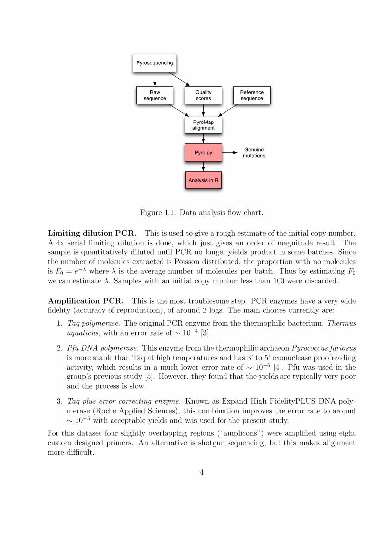
Raw sequence

Quality scores

Reference sequence

PyroMap alignment

Pyrosequencing

Pyro.py

Analysis in R

Genuine mutations

Figure 1.1: Data analysis flow chart.

Limiting dilution PCR. This is used to give a rough estimate of the initial copy number.A 4x serial limiting dilution is done, which just gives an order of magnitude result. Thesample is quantitatively diluted until PCR no longer yields product in some batches. Sincethe number of molecules extracted is Poisson distributed, the proportion with no moleculesis F0 = e−λ where λ is the average number of molecules per batch. Thus by estimating F0

we can estimate λ. Samples with an initial copy number less than 100 were discarded.

Amplification PCR. This is the most troublesome step. PCR enzymes have a very widefidelity (accuracy of reproduction), of around 2 logs. The main choices currently are:

1. Taq polymerase. The original PCR enzyme from the thermophilic bacterium, Thermus

aquaticus, with an error rate of ∼ 10−4 [3].

2. Pfu DNA polymerase. This enzyme from the thermophilic archaeon Pyrococcus furiosus

is more stable than Taq at high temperatures and has 3’ to 5’ exonuclease proofreadingactivity, which results in a much lower error rate of ∼ 10−6 [4]. Pfu was used in thegroup’s previous study [5]. However, they found that the yields are typically very poorand the process is slow.

3. Taq plus error correcting enzyme. Known as Expand High FidelityPLUS DNA poly-merase (Roche Applied Sciences), this combination improves the error rate to around∼ 10−5 with acceptable yields and was used for the present study.

For this dataset four slightly overlapping regions (“amplicons”) were amplified using eightcustom designed primers. An alternative is shotgun sequencing, but this makes alignmentmore difficult.

4

Dilution. Following amplification it is necessary to dilute the DNA down so there is justone molecule per bead. Amplification followed by dilution seems wasteful, so in the futureit is hoped a more direct method could be developed.

Pyrosequencing. Around 25 to 30 samples are run on one plate. Errors here are less likelyto be a problem than in the initial PCR because the PCR in the pyrosequencing processwill only result in an observed error if a mismatch occurs in the first round: otherwise theerroneous signal will be hidden by the stronger true signal.

1.2 Analysis issues

Aligning the 454 reads is simplified because the HBV genome is known. The group foundthat straightforward Smith-Waterman (SW) alignment had problems with the common phe-nomenon of an insertion closely followed by a deletion (up to around 6bp away), because thescore across the small gap is not very significant. The group developped Asymmetric SW [5],which takes into account the quality scores from the pyrosequencer, and helped to alleviatethis issue. A further development was the Python based alignment program “Pyromap”which also weights the Sanger sequence. Pyromap is used upstream of my analysis.

The greatest concern is the accuracy of the initial PCR, especially if there are early stageerrors: these are the most likely to look like true variants. In the group’s previous UDPSstudy on HIV-1 [5], a Poisson distribution on errors was used in the homopolymeric andnon-homopolymeric regions, which was fitted by Expectation Maximisation (EM). However,the increased error rate for the Taq blend seems to result in early errors getting replicatedand this results in the error distribution no longer being Poisson.

5

Chapter 2

Statistical Analysis of Plasmid

Controls

In order to detect which signals in the data represent genuine variants it is necessary to char-acterise the errors resulting from amplification and pyrosequencing. To facilitate this, threewell characterised HBV plasmid vectors were pyro-sequenced using the same experimentalmethod as the patient samples (although the initial copy number was significantly higher,around 100,000). Deviations from the consensus sequence represent either errors occurringduring the PCR or the pyrosequencing itself. This data allows us to fit a distribution underthe hypothesis that no minor variants are present, which can then be tested. Determiningwhat parametric form this null distribution should take depends on the characteristics ofthe PCR and sequencing errors, which are analysed in this section. The typical process forthis analysis was to develop Python code to manipulate and analyse the aligned read dataand output the results in a format easily readable by the statistical programming languageR, which was then used for further analysis and plotting.

The level of coverage over the three plasmid controls varies significantly from around 160to 10,000, with mean just over 3000. Possibly due to primer binding issues, one of the fouramplicons is amplified poorly, resulting in low coverage over a significant region.

2.1 Error distribution

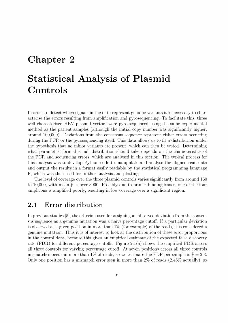
In previous studies [5], the criterion used for assigning an observed deviation from the consen-sus sequence as a genuine mutation was a naive percentage cutoff. If a particular deviationis observed at a given position in more than 1% (for example) of the reads, it is considered agenuine mutation. Thus it is of interest to look at the distribution of these error proportionsin the control data, because this gives an empirical estimate of the expected false discoveryrate (FDR) for different percentage cutoffs. Figure 2.1(a) shows the empirical FDR acrossall three controls for varying percentage cutoff. At seven positions across all three controlsmismatches occur in more than 1% of reads, so we estimate the FDR per sample is 7

3= 2.3.

Only one position has a mismatch error seen in more than 2% of reads (2.45% actually), so

6

at this threshold the FDR is reduced to around 13. A simple improvement I made to this

basic analysis was to consider mismatches going to different nucleotides separately, whichmakes a significant difference for the worst errors: for example, what appears to be an errorfrequency of 4.2% is actually a mismatch to A at 1.7% and to C at 2.4%.

(a) Empirical estimate of FDR versus percentagecutoff.

(b) Error rate against number of ambiguous basecalls.

Figure 2.1: Statistical analysis of plasmid control data.

2.2 Homopolymeric regions

454 pyrosequencing is known to be particularly error prone in homopolymeric regions dueto carry forward and incomplete extension (CAFIE) errors [2]. Incomplete extension iswhen the homopolymer is not completed due to insufficient dNTPs. Carry forward errorsoccur when a nucleotide from the end of a homopolymer is read a few bases later on due toincomplete dNTP flushing. For example, if the true sequence is AAAATCG, it may be readas AAATCGA. We define a homopolymeric region as three or more identical nucleotides andthe immediately flanking non-identical nucleotides.

Table 2.1 summarises the error rate for mismatch vs. indels and context. I found a criticalbug in the existing code for calculating these error rates that counted a single mismatch errorfour times. I found that the mismatch error rate is not significantly affected by whether theregion is homopolymeric. The increase in the overall error rate in homopolymeric regions isdue only to the increase in indel rate (the number of ambiguous base calls, N, is small).

2.3 Quality scores

The quality scores from the pyrosequencing software relate to the probability of CAFIEerrors, which is somewhat different to Sanger sequencing phred scores. There is a significant

7

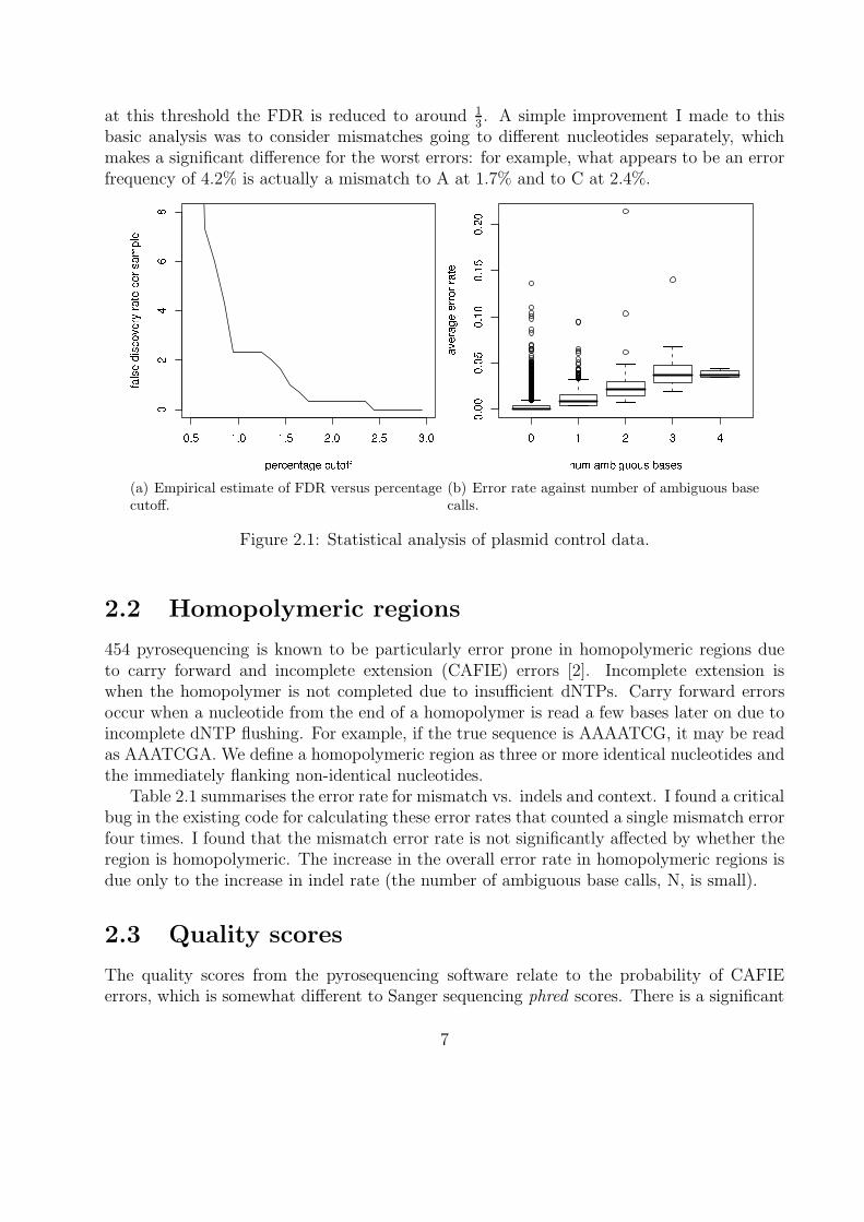
Error rate/10−3 Mismatch Indel N OverallHomopolymeric 1.125 2.98 1.87 1.811Non-homopolymeric 1.126 1.76 1.11 1.298Overall 1.126 2.29 1.32 1.487

Table 2.1: Context specific and non-specific mismatch, indel and overall error rates averagedacross the three controls.

correlation (p < 0.05) between the mismatch error rate and average quality score, but theeffect size is very small: the gradient is −1.2 × 10−5. I also investigated whether at a givenposition with mismatch errors the quality score was lower for the specific incorrect base calls,but found no significant effect (results not shown).

2.4 Error distribution over reads

A previous study [6] into the error rates of massively parallel pyrosequencing found thata small number of poor quality reads contained a disproportionate percentage of the totalerrors. Although this phenomenon seems less severe for our data set, I found the worst 2%of reads still account for 20% of errors. In [6] they also found that reads with lengths outsidethe main peaks had increased error rate, which I confirmed in our data set. Figure 2.1(b)shows the strong correlation between the error rate and the number of ambiguous base callsin a read. Note that only 2% of reads contain any ambiguous base calls, so discarding these isrecommended. I found the correlation is statistically significant (p < 0.001) between the errorrate and average quality score across a read but the effect size is very small (β = −1.2×10−3).

2.5 Mismatch rates

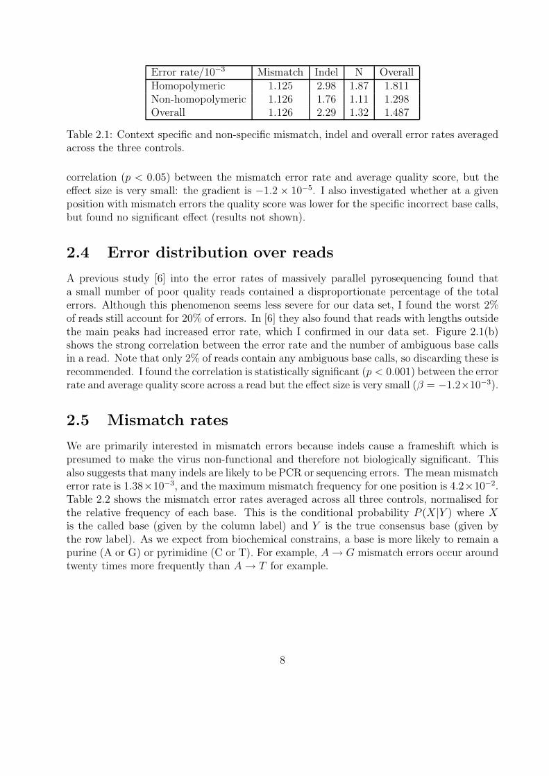
We are primarily interested in mismatch errors because indels cause a frameshift which ispresumed to make the virus non-functional and therefore not biologically significant. Thisalso suggests that many indels are likely to be PCR or sequencing errors. The mean mismatcherror rate is 1.38×10−3, and the maximum mismatch frequency for one position is 4.2×10−2.Table 2.2 shows the mismatch error rates averaged across all three controls, normalised forthe relative frequency of each base. This is the conditional probability P (X|Y ) where X

is the called base (given by the column label) and Y is the true consensus base (given bythe row label). As we expect from biochemical constrains, a base is more likely to remain apurine (A or G) or pyrimidine (C or T). For example, A → G mismatch errors occur aroundtwenty times more frequently than A → T for example.

8

A G T CA 9.99e-01 1.39e-03 7.12e-05 3.39e-05G 4.53e-04 9.99e-01 3.22e-04 1.87e-05T 1.69e-04 3.73e-05 9.98e-01 1.54e-03C 4.14e-04 4.74e-05 4.10e-04 9.99e-01

Table 2.2: Normalised mismatch error rates across controls.

2.6 Error rate along read

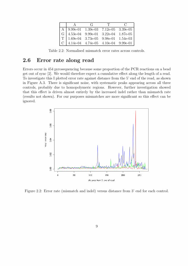
Errors occur in 454 pyrosequencing because some proportion of the PCR reactions on a beadget out of sync [2]. We would therefore expect a cumulative effect along the length of a read.To investigate this I plotted error rate against distance from the 5’ end of the read, as shownin Figure A.3. There is significant noise, with systematic peaks appearing across all threecontrols, probably due to homopolymeric regions. However, further investigation showedthat this effect is driven almost entirely by the increased indel rather than mismatch rate(results not shown). For our purposes mismatches are more significant so this effect can beignored.

Figure 2.2: Error rate (mismatch and indel) versus distance from 3’ end for each control.

9

2.7 Analytic distributions

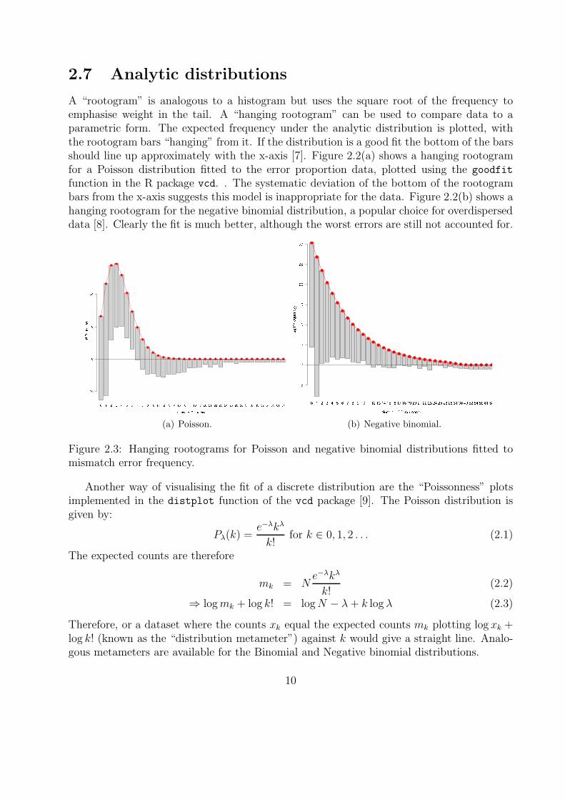
A “rootogram” is analogous to a histogram but uses the square root of the frequency toemphasise weight in the tail. A “hanging rootogram” can be used to compare data to aparametric form. The expected frequency under the analytic distribution is plotted, withthe rootogram bars “hanging” from it. If the distribution is a good fit the bottom of the barsshould line up approximately with the x-axis [7]. Figure 2.2(a) shows a hanging rootogramfor a Poisson distribution fitted to the error proportion data, plotted using the goodfit

function in the R package vcd. . The systematic deviation of the bottom of the rootogrambars from the x-axis suggests this model is inappropriate for the data. Figure 2.2(b) shows ahanging rootogram for the negative binomial distribution, a popular choice for overdisperseddata [8]. Clearly the fit is much better, although the worst errors are still not accounted for.

(a) Poisson. (b) Negative binomial.

Figure 2.3: Hanging rootograms for Poisson and negative binomial distributions fitted tomismatch error frequency.

Another way of visualising the fit of a discrete distribution are the “Poissonness” plotsimplemented in the distplot function of the vcd package [9]. The Poisson distribution isgiven by:

Pλ(k) =e−λkλ

k!for k ∈ 0, 1, 2 . . . (2.1)

The expected counts are therefore

mk = Ne−λkλ

k!(2.2)

⇒ log mk + log k! = log N − λ + k log λ (2.3)

Therefore, or a dataset where the counts xk equal the expected counts mk plotting log xk +log k! (known as the “distribution metameter”) against k would give a straight line. Analo-gous metameters are available for the Binomial and Negative binomial distributions.

10

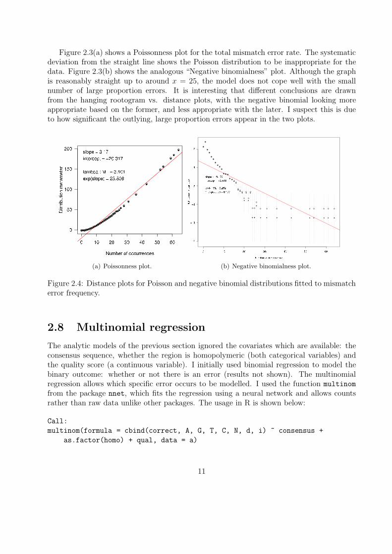
Figure 2.3(a) shows a Poissonness plot for the total mismatch error rate. The systematicdeviation from the straight line shows the Poisson distribution to be inappropriate for thedata. Figure 2.3(b) shows the analogous “Negative binomialness” plot. Although the graphis reasonably straight up to around x = 25, the model does not cope well with the smallnumber of large proportion errors. It is interesting that different conclusions are drawnfrom the hanging rootogram vs. distance plots, with the negative binomial looking moreappropriate based on the former, and less appropriate with the later. I suspect this is dueto how significant the outlying, large proportion errors appear in the two plots.

(a) Poissonness plot. (b) Negative binomialness plot.

Figure 2.4: Distance plots for Poisson and negative binomial distributions fitted to mismatcherror frequency.

2.8 Multinomial regression

The analytic models of the previous section ignored the covariates which are available: theconsensus sequence, whether the region is homopolymeric (both categorical variables) andthe quality score (a continuous variable). I initially used binomial regression to model thebinary outcome: whether or not there is an error (results not shown). The multinomialregression allows which specific error occurs to be modelled. I used the function multinom

from the package nnet, which fits the regression using a neural network and allows countsrather than raw data unlike other packages. The usage in R is shown below:

Call:

multinom(formula = cbind(correct, A, G, T, C, N, d, i) ~ consensus +

as.factor(homo) + qual, data = a)

11

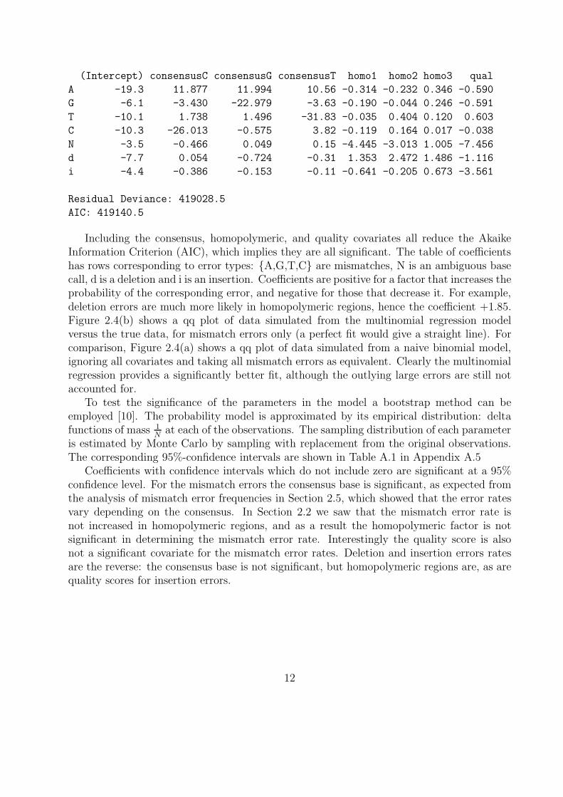
(Intercept) consensusC consensusG consensusT homo1 homo2 homo3 qual

A -19.3 11.877 11.994 10.56 -0.314 -0.232 0.346 -0.590

G -6.1 -3.430 -22.979 -3.63 -0.190 -0.044 0.246 -0.591

T -10.1 1.738 1.496 -31.83 -0.035 0.404 0.120 0.603

C -10.3 -26.013 -0.575 3.82 -0.119 0.164 0.017 -0.038

N -3.5 -0.466 0.049 0.15 -4.445 -3.013 1.005 -7.456

d -7.7 0.054 -0.724 -0.31 1.353 2.472 1.486 -1.116

i -4.4 -0.386 -0.153 -0.11 -0.641 -0.205 0.673 -3.561

Residual Deviance: 419028.5

AIC: 419140.5

Including the consensus, homopolymeric, and quality covariates all reduce the AkaikeInformation Criterion (AIC), which implies they are all significant. The table of coefficientshas rows corresponding to error types: {A,G,T,C} are mismatches, N is an ambiguous basecall, d is a deletion and i is an insertion. Coefficients are positive for a factor that increases theprobability of the corresponding error, and negative for those that decrease it. For example,deletion errors are much more likely in homopolymeric regions, hence the coefficient +1.85.Figure 2.4(b) shows a qq plot of data simulated from the multinomial regression modelversus the true data, for mismatch errors only (a perfect fit would give a straight line). Forcomparison, Figure 2.4(a) shows a qq plot of data simulated from a naive binomial model,ignoring all covariates and taking all mismatch errors as equivalent. Clearly the multinomialregression provides a significantly better fit, although the outlying large errors are still notaccounted for.

To test the significance of the parameters in the model a bootstrap method can beemployed [10]. The probability model is approximated by its empirical distribution: deltafunctions of mass 1

Nat each of the observations. The sampling distribution of each parameter

is estimated by Monte Carlo by sampling with replacement from the original observations.The corresponding 95%-confidence intervals are shown in Table A.1 in Appendix A.5

Coefficients with confidence intervals which do not include zero are significant at a 95%confidence level. For the mismatch errors the consensus base is significant, as expected fromthe analysis of mismatch error frequencies in Section 2.5, which showed that the error ratesvary depending on the consensus. In Section 2.2 we saw that the mismatch error rate isnot increased in homopolymeric regions, and as a result the homopolymeric factor is notsignificant in determining the mismatch error rate. Interestingly the quality score is alsonot a significant covariate for the mismatch error rates. Deletion and insertion errors ratesare the reverse: the consensus base is not significant, but homopolymeric regions are, as arequality scores for insertion errors.

12

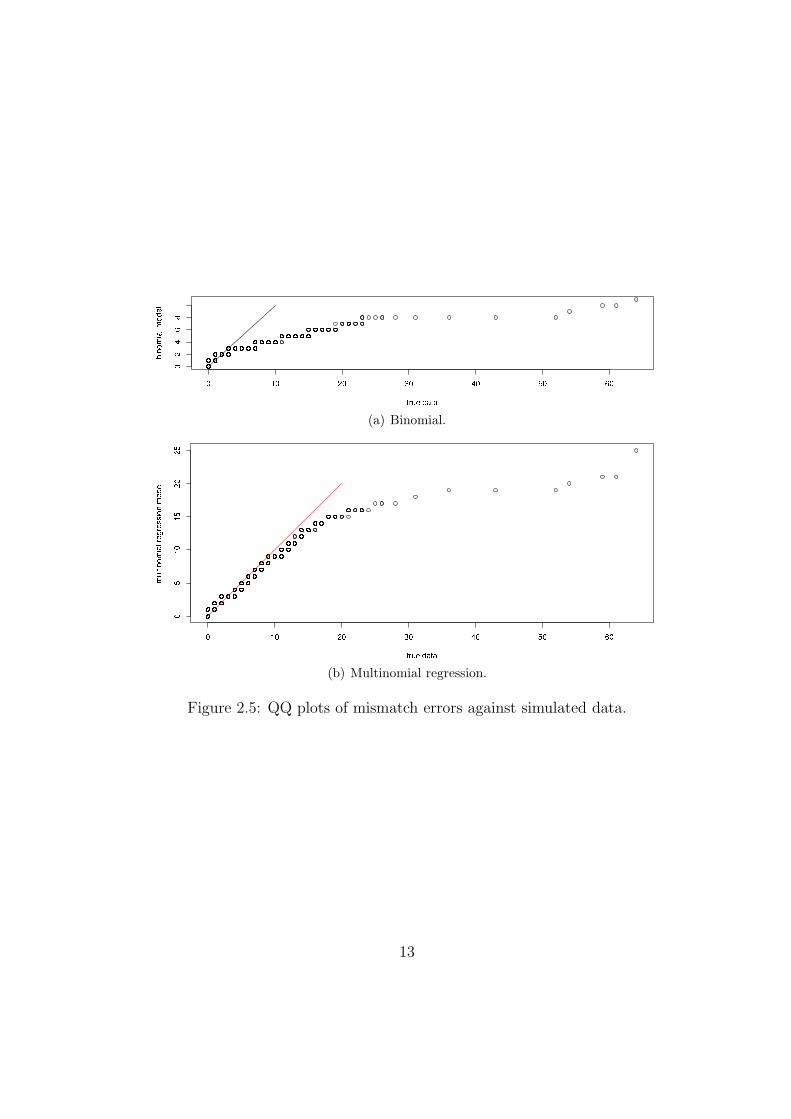
(a) Binomial.

(b) Multinomial regression.

Figure 2.5: QQ plots of mismatch errors against simulated data.

13

Chapter 3

PCR Simulation

A concern is whether early cycle amplification PCR errors could be amplified to a significantproportion of the population and then resemble a genuine minor variant. This will dependon the initial copy number. Since the plasmid controls had initial copy numbers on theorder of 100,000, compared to just 100-1000 for the samples, they cannot be used to answerthis question. In order to model the probability of this occuring and the resulting errordistribution, I ran computer simulations of the PCR amplification process with a simplebinary mutation model. I wrote the simulation algorithm in C for performance reasons.

3.1 Computer simulation

I modelled the PCR amplification process as a simple autocatalytic reaction, using a stochas-tic simulation algorithm where each step corresponds to a PCR cycle. The reaction is initiallyexponential as the number of DNA molecules increases, and then becomes limited by theavailability of dNTPs. New DNA molecules inherit mutations from their parent molecule,and gain new mutations at random at a specified rate. The simulated molecules are repre-sented as a N×M binary matrix, where N is the length of the sequence and M is the numberof individual molecules. Each column represents a molecule. Although the final populationsize varies slightly depending on the initial population, it was typically 6000-8000.

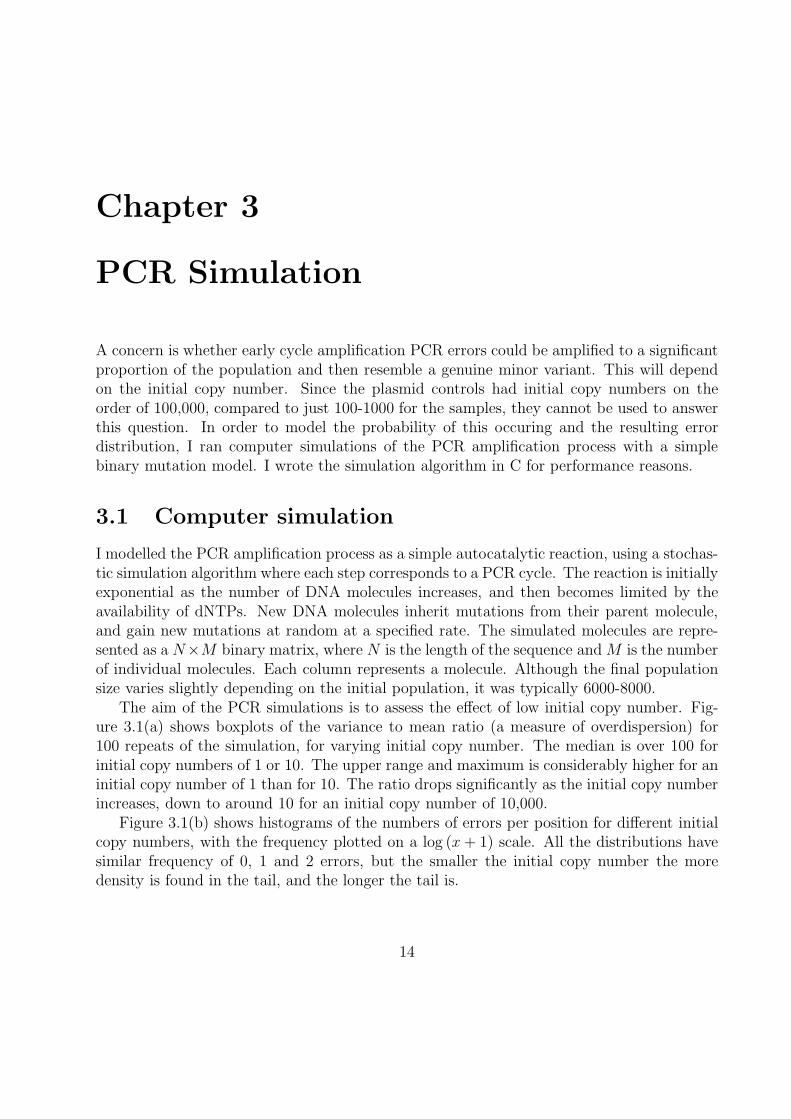
The aim of the PCR simulations is to assess the effect of low initial copy number. Fig-ure 3.1(a) shows boxplots of the variance to mean ratio (a measure of overdispersion) for100 repeats of the simulation, for varying initial copy number. The median is over 100 forinitial copy numbers of 1 or 10. The upper range and maximum is considerably higher for aninitial copy number of 1 than for 10. The ratio drops significantly as the initial copy numberincreases, down to around 10 for an initial copy number of 10,000.

Figure 3.1(b) shows histograms of the numbers of errors per position for different initialcopy numbers, with the frequency plotted on a log (x + 1) scale. All the distributions havesimilar frequency of 0, 1 and 2 errors, but the smaller the initial copy number the moredensity is found in the tail, and the longer the tail is.

14

(a) Variance to mean ratio. (b) Histograms.

Figure 3.1: Error distribution from PCR with different initial copy numbers.

3.2 Sparse matrix representation

In my initial implementation the limiting factor in the size of the simulations was the memoryrequirements. Because stochastic effects are size dependent, it is important for the scalesimulation to be as close as possible to the scale of the real reaction. To allow a muchlarger simulation to be run, a sparse representation of the binary N × M mutation matrixis required. To do this two arrays, B and C, are defined:

1. Element i of array C gives the row index, i.e. position in the sequence, of the ithmutation. C has length equal to the number of mutations.

2. Element j of array B gives the index in C of the first mutation in column j. B haslength M + 1.

So C[B[i], · · · , B[i + 1] − 1] are the positions of the mutations in individual i, which hasB[i + 1] − B[i] mutations.

Using this sparse matrix representation it is possible to run considerably larger, morerealistic simulations, up to final populations of around 109. To mirror the dilution of thePCR product onto beads for pyrosequencing, 5000 “molecules” are sampled at random fromthis large initial population. This is repeated 100 times to make best use of the informationabout the final population. Note that the number of repeats was varied depending on theinitial copy number n0. If the error rate is ǫ and there are M positions at which mutationscan occur, the expected number of mutations in the first round of replication is ǫn0M ,assuming that all the molecules get duplicated. To see the effect of these first round errors,enough repeats need to be run to them. The number of repeats is therefore set to be 10

ǫn0M

(rounded up), so that the expected number of first cycle errors observed is 10 (a minimumof 10 repeats is also specified for the larger initial copy numbers).

15

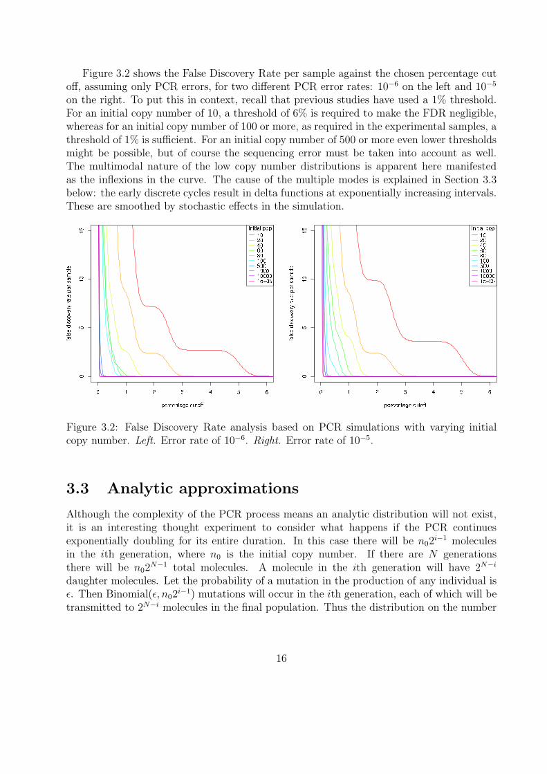
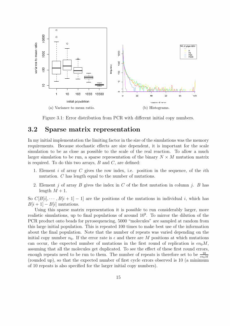
Figure 3.2 shows the False Discovery Rate per sample against the chosen percentage cutoff, assuming only PCR errors, for two different PCR error rates: 10−6 on the left and 10−5

on the right. To put this in context, recall that previous studies have used a 1% threshold.For an initial copy number of 10, a threshold of 6% is required to make the FDR negligible,whereas for an initial copy number of 100 or more, as required in the experimental samples, athreshold of 1% is sufficient. For an initial copy number of 500 or more even lower thresholdsmight be possible, but of course the sequencing error must be taken into account as well.The multimodal nature of the low copy number distributions is apparent here manifestedas the inflexions in the curve. The cause of the multiple modes is explained in Section 3.3below: the early discrete cycles result in delta functions at exponentially increasing intervals.These are smoothed by stochastic effects in the simulation.

Figure 3.2: False Discovery Rate analysis based on PCR simulations with varying initialcopy number. Left. Error rate of 10−6. Right. Error rate of 10−5.

3.3 Analytic approximations

Although the complexity of the PCR process means an analytic distribution will not exist,it is an interesting thought experiment to consider what happens if the PCR continuesexponentially doubling for its entire duration. In this case there will be n02

i−1 moleculesin the ith generation, where n0 is the initial copy number. If there are N generationsthere will be n02

N−1 total molecules. A molecule in the ith generation will have 2N−i

daughter molecules. Let the probability of a mutation in the production of any individual isǫ. Then Binomial(ǫ, n02

i−1) mutations will occur in the ith generation, each of which will betransmitted to 2N−i molecules in the final population. Thus the distribution on the number

16

of times, x, a mutation is duplicated is given by:

f(x|N, n0, ǫ) =1

Z(M, N0, ǫ

N∑

r=2

ǫn02r−1δ(x − 2N−r) (3.1)

Since n0 and ǫ are just factors we can absorb them into the normalisation constant, whichis easily calculated as the sum of a finite geometric series: Z(N) = 2N − 2. The mean isstraightforward to calculate:

Ex = (N − 1)2N−1

2N − 2(3.2)

To calculate the variance we also need E[x2] = 2N−2. The variance is then given by thestandard formula var(x) = E[x2] − (Ex)2. The mean, variance and variance to mean ratiofor a range of values of N are shown in Figure A.4.

Figure 3.3: Mean, variance and variance over mean ratio for varying number of generationsfor exponential PCR model.

17

Chapter 4

Classifying genuine mutations

The simplest method to classify a mismatch as a genuine mutation is to use a percentagecutoff: if the mismatch occurs in more than 1% of reads, for example, classify it as genuine.In this section we develop two more sophisticated methodologies which leverage results fromChapter 2. The first is an essentially frequentist hypothesis testing approach, and the secondis a more Bayesian mixture model approach. Since for mismatch error rates we have foundthat the quality score and homopolymeric state are not significant, we now focus on robustestimation of the 4 by 4 nucleotide transition matrix, Θ, which will be required for bothmethods.

4.1 Estimating the nucleotide transition matrix

Element (i, j) of Θ gives the probability of observing nucleotide j, given that the truenucleotide was i. A sufficient statistic for Θ is the count matrix of nucleotide mismatcherrors observed in the controls, n. Element (i, j) of n is the number of times we observenucleotide j, when the consensus nucleotide was i. Each row of the n is a sample from amultinomial distribution with parameters given by the corresponding row of Θ. Thus thelikelihood function for a row i is:

P (ni.|Θi.) =∏

j

Θnij

ij (4.1)

So the total likelihood function is

P (n|Θ) =∏

i,j

Θnij

ij (4.2)

The maximum likelihood estimate of Θ is simply the normalised count matrix:

ΘMLij =

nij∑

k nkj

(4.3)

To prevent overfitting it would be better to calculate the posterior distribution of Θ, given thedata. To achieve this we must specify a prior on Θ. The conjugate prior to the multinomial

18

distribution is the Dirichlet distibution. Therefore we specify each row i of Θ to be drawnfrom a Dirichlet distribution with parameter vector αi. Thus:

P (Θi.|αi) =Γ(∑

j αij)∏

j Γ(αij)

∏

j

Θαij−1ij (4.4)

The four vectors form a matrix α, whose form is restricted as follows:

αij =

{

a if i = j

b if i 6= j(4.5)

Intuitively we are saying that a prior we do not expect any particular mismatch to be morelikely than another, and but the the probability of no mismatch is of course different. Analternative not investigated here would be to have different prior parameters for transitionvs. transversion mismatches. We can now express the prior on Θ in terms of a and b:

P (Θ|a, b) =∏

i

P (Θi.|a, b) (4.6)

=Γ(a + 3b)4

Γ(b)12Γ(a)4

∏

i

Θa−1ii

∏

j,j 6=i

Θb−1ij (4.7)

The joint distribution over the data D and Θ can now be expressed:

P (D,Θ|a, b) = P (D|Θ, a, b)P (Θ|a, b) (4.8)

=Γ(a + 3b)4

Γ(b)12Γ(a)4

∏

i

Θnii+a−1ii

∏

j,j 6=i

Θnij+b−1ij (4.9)

Note that from the form of the posterior it is clear that the maximum a posterior (MAP)estimate of Θ is

ΘMAPij =

nij + αij∑

k(nkj + αkj)(4.10)

because nij +αij is the effective number of counts of nucleotide i going to j. We can estimatea and b using the evidence framework where we maximise P (D|a, b), a Type II maximumlikelihood method [11].

P (D|a, b) =

∫

P (D,Θ|a, b)dΘ

=Γ(a + 3b)4

Γ(b)12Γ(a)4

∏

i

∫ 1

0

Θnii+a−1ii

∏

j,j 6=i

Θnij+b−1ij dΘi

=Γ(a + 3b)4

Γ(b)12Γ(a)4

∏

i

Γ(nii + a)∏

j 6=i Γ(nij + b)

Γ(nii + a +∑

j 6=i(nij + b))

19

It will be easier to maximise the log evidence:

log P (D|a, b) = 4 log Γ(a + 3b) − 12 log Γ(b) − 4 log Γ(a) +

∑

i

(

log Γ(nii + a) +∑

j 6=i

log Γ(nij + b) − log Γ(nii + a +∑

j 6=i

(nij + b))

)

To find the minimum of this function with respect to a and b a Newton-Raphson schemeis used, for which the gradient, g, and Hessian matrix, H, are required. To calculate thegradient the digamma function, defined by Ψ(x) = d

dxlog Γ(x) is useful. The Hessian will be

in terms of the trigamma function Ψ′(x) = dΨ(x)dx

. The details are somewhat laborious, butcan be found in the Appendix. The Newton Raphson iteration is:

xn+1 = xn − λH−1g (4.11)

where x = (a, b)T and λ < 1 is used to help ensure stability.

4.2 Method 1: Hypothesis testing

Once an estimate of the nucleotide transition matrix Θ is available the probability of aspecific error under the model can be calculated. If we have a position where the consensusnucleotide is i but nucleotide j is observed ne times out of a coverage of n, then the probabilityof this occurring is given by the Binomial distribution, since this is the marginal distributionof a multinomial.

P (nij = ne|Θ) =

(

n

ne

)

Θne

ij (1 − Θij)n−ne (4.12)

The maximum likelihood or MAP estimate could be used, but it is preferred to integrateover Θ using the posterior distribution. Let βij = nij +αij be the parameters of the posteriorDirichlet distribution over Θ. The marginal distribution of Θij is then a Beta distributionwith parameters (βij, βi0 − βij), where βi0 =

∑

j βij , i.e.

P (Θij|β) =1

B(βij, βi0 − βij)Θ

βij−1ij (1 − Θij)

βi0−βij−1 (4.13)

where the normalising constant, B(., .) is the Beta function. To integrate over Θ:

P (nij = ne|β) =

∫

P (nij = ne|Θ)P (Θij|β)dΘij (4.14)

=1

B(βij , βi0 − βij)

(

n

ne

)∫

Θne+βij−1ij (1 − Θij)

n−ne+βi0−βij−1dΘij(4.15)

=

(

n

ne

)

B(ne + βij, n − ne + βi0 − βij)

B(βij , βi0 − βij)(4.16)

Since it is possible to perform this integration analytically there is little additional compu-tational cost compared to using the simple MAP estimate. This expression calculates the

20

probability of observing ne mismatches. We classify genuine mutations as mismatches wherethis probability is lower than some threshold (call this the “likelihood” method), but it ismore rigorous to calculate a p-value for each mismatch: the probability of this event, or any

more extreme event, under the null hypothesis; in this case P (nij ≥ ne|β). Since we usuallyhave ne ≪ n it will be cheaper to calculate the p-value as follows:

P (nij ≥ ne|β) = 1 − P (nij < ne|β) (4.17)

= 1 −

ne−1∑

m=0

P (nij = m|β) (4.18)

where each term in the sum is evaluated according to Equation 4.16. If the p-value is lessthan the required significance level then the mismatch is classified as a genuine mutation.Calculating this sum can be quite computationally intensive for large n and moderate ne, soI used the Python package ctypes to interface to compiled, optimised C code to calculatethe Binomial coefficients (see Appendix A.7).

4.3 Method 2: A mixture model

The observed mismatches are generated by two processes: PCR/sequencing errors and gen-uine mutations. A mixture model can be used to represent this, where the mixture propor-tions correspond to the probability a particular mismatch is a genuine mutation rather thanan error. Mixture models can be fitting using the Expectation Maximisation method, whichiterates between fitting the mixing proportions and model parameters. Using the controlsthe error model can be fitted as described in Section 4.1. To model the genuine mutationswe will use a codon mismatch matrix, since allows the incorporation three desirable features:

1. Synonymous mutations which do not affect the resulting amino acid are more likelythan non-synonymous mutations. Mutations in the third base of a codon are the mostlikely to be synonymous, leading to the idea of third base “wobble”.

2. Non-synonymous mutations which result in amino acids with different physiochemicalproperties, such as polarity, are less likely because they are more probable to interferewith protein function.

3. Mutations which result in a stop codon are very unlikely to be genuine because theshortened protein will be non-functional.

The reading frame is known for the consensus sequence, so it does not need to be inferred.The number of parameters in the codon model, 642 = 4096, is very large so the risk ofoverfitting is severe. To avoid this we should use the MAP estimation of the transitionmatrix, or better still estimate the posterior. The equations are exactly the same as for thenucleotide mismatch matrix, only now the indices are over all codons rather than nucleotides.

21

Expectation step. This involves calculating the latent variables, which in this case arethe mixture proportions. Let mi be a binary latent variable equal to 1 if codon mismatchi is a genuine mutation, and equal to 0 if it is an error. To calculate the probability thatmismatch i is a genuine mutation, πi, we use Bayes’ rule assuming equal priors (i.e. mutationand error are equally likely a prior):

πi = P (mi = 1|Di, Θerror, Θmutation) =P (Di|mi = 1, Θmutation)

P (Di|mi = 1, Θmutation) + P (Di|mi = 0, Θerror)(4.19)

where Di is the data associated with mismatch i (i.e. reference and query codon, howmany repeats and coverage), and Θmutation and Θerror are the current estimates of the codontransition matrix for the mutation and error models respectively.

Maximisation step. This step involves updating the Θmutation using the mixing propor-tions calculated in the previous step. The count used now are a weighted sum, with theweights given by the mixing proportions.

nij =

{∑

k nk1(rk = i, qk = j) if i = j∑

k nkπk1(rk = i, qk = j) if i 6= j(4.20)

where rk and qk are the reference and query codons respectively for mutation k, 1(·) is 1 ifthe statement is true and nk is the number of times this codon mismatch is observed. Notethat for counting the number of times mismatches do not not occur for a codon, the mixingproportion is effectively 1 since neither a mutation nor an error has occurred.

4.4 Classification performance

Assessing classification performance is difficult because no ground truth results are available:which mismatches really are genuine mutations? Limiting dilution Sanger sequencing resultsare available for one of the samples however. This method is not able to detect minorvariants at very low levels, so some genuine mutants will not have been detected. Never-the-less, this is the closest to ground truth available for comparing the classification methods.The data consists of 95 sequences, which I aligned to the 454 consensus sequence using theclustalw2 multiple sequence alignment tool [12]. By varying the appropriate thresholds aReceiver Operator Characteristic (ROC) curve (true positive rate against false positive rate,see Appendix A.8 for definitions) can be produced for each method, as shown in Figure 4.1.Better performance is indicated by being closer to the top left corner. Since some genuinemutations will be missing from the “ground truth” set, the number of false positives will beover-estimated and the number of true positives under-estimated, giving a pessimistic viewof the performance of these methods. However, the results can still be used to assess therelative performance of the methods.

The more sophisticated methods outperform the percentage cutoff along most of thecurve. Somewhat surprisingly, the mixture model performs worse than the p-value and

22

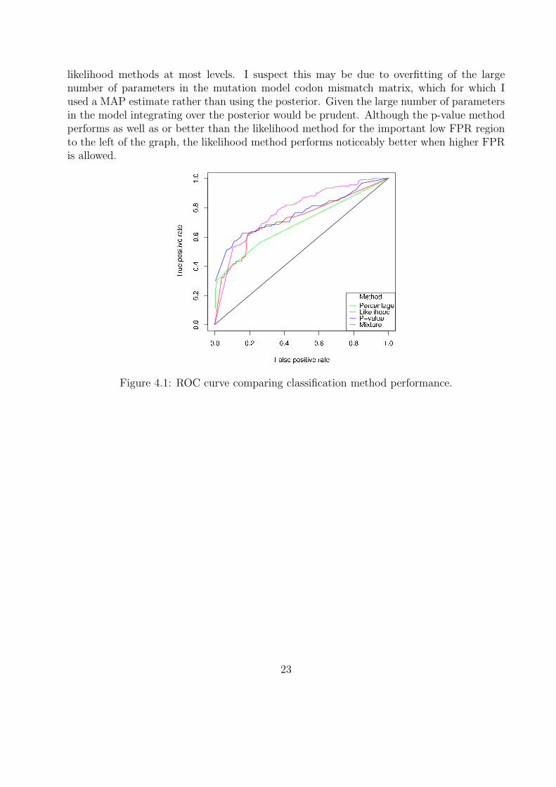
likelihood methods at most levels. I suspect this may be due to overfitting of the largenumber of parameters in the mutation model codon mismatch matrix, which for which Iused a MAP estimate rather than using the posterior. Given the large number of parametersin the model integrating over the posterior would be prudent. Although the p-value methodperforms as well as or better than the likelihood method for the important low FPR regionto the left of the graph, the likelihood method performs noticeably better when higher FPRis allowed.

Figure 4.1: ROC curve comparing classification method performance.

23

Chapter 5

Conclusion

I have statistically characterised the errors inherent in 454 pyrosequencing, and used the re-sults to design methods for detecting genuine variants which outperform the naive thresholdmethod commonly used. The code necessary to run these classification methods is containedin a Python module, pyro, which I will make publicly available. I have used computer sim-ulations of the PCR to help understand how initial copy number determines the probabilityof false positives resulting from early cycle errors. Appendices A.2 and A.3 show some otheranalyses not directly related to my main project.

There are various avenues of further work I would like to explore. As mentioned inSection 4.4, the somewhat disappointing performance of the mixture model maybe due tooverfitting of the large parameter mutation model. To overcome this integration over theposterior of the codon transition matrix should be performed, rather than using a MAPestimate. This would require the beta function in Python, which is available as part of thetranscendental module. A more ambitious aim would be to incorporate more multivariateinformation into the classification methods. For example, if two mismatches always co-occur, it is highly unlikely they are errors but feasible that they both occur in the sameminor variant. A simple way to assess this would be to calculate a co-occurence table ofthe most frequent errors. A more computationally intensive method would be to attempt toinfer the hidden phylogeny of the minor variants. Both these methods are complicated bythe fact that the sequences only cover some of the region of interest. Each amplicon wouldhave to be considered separately, but the phylogenies would need to be consistent withineach.

24

Bibliography

[1] Bndicte Roquebert, Isabelle Malet, Marc Wirden, Roland Tubiana, Marc-AntoineValantin, Anne Simon, Christine Katlama, Gilles Peytavin, Vincent Calvez, and Anne-Genevive Marcelin. Role of hiv-1 minority populations on resistance mutational patternevolution and susceptibility to protease inhibitors. AIDS, 20(2):287–289, Jan 2006.

[2] Marcel Margulies, Michael Egholm, William E Altman, Said Attiya, Joel S Bader, andJonathan M Rothberg. Genome sequencing in microfabricated high-density picolitrereactors. Nature, 437(7057):376–380, Sep 2005.

[3] K. A. Eckert and T. A. Kunkel. High fidelity dna synthesis by the thermus aquaticusdna polymerase. Nucleic Acids Res, 18(13):3739–3744, Jul 1990.

[4] K. S. Lundberg, D. D. Shoemaker, M. W. Adams, J. M. Short, J. A. Sorge, and E. J.Mathur. High-fidelity amplification using a thermostable dna polymerase isolated frompyrococcus furiosus. Gene, 108(1):1–6, Dec 1991.

[5] Chunlin Wang, Yumi Mitsuya, Baback Gharizadeh, Mostafa Ronaghi, and Robert WShafer. Characterization of mutation spectra with ultra-deep pyrosequencing: applica-tion to hiv-1 drug resistance. Genome Res, 17(8):1195–1201, Aug 2007.

[6] Susan M Huse, Julie A Huber, Hilary G Morrison, Mitchell L Sogin, and David MarkWelch. Accuracy and quality of massively parallel dna pyrosequencing. Genome Biol,8(7):R143, 2007.

[7] Howard Wainer. The suspended rootogram and other visual displays: An empiricalvalidation. The American Statistician, 28(4):143–145, 1974.

[8] Kenneth W. Church and William A. Gale. Poisson mixtures. Natural Language Engi-

neering, 1:163–190, 1995.

[9] David C. Hoaglin. A poissonness plot. The American Statistician, 34(3):146–149, 1980.

[10] B. Efron. Bootstrap methods: Another look at the jackknife. The Annals of Statistics,7(1):1–26, 1979.

[11] D. J. C. Mackay. Bayesian methods for adaptive models. PhD thesis, California Instituteof Technology, 1991.

25

[12] M. A. Larkin, G. Blackshields, N. P. Brown, R. Chenna, P. A. McGettigan,H. McWilliam, F. Valentin, I. M. Wallace, A. Wilm, R. Lopez, J. D. Thompson,T. J. Gibson, and D. G. Higgins. Clustal w and clustal x version 2.0. Bioinformat-

ics, 23(21):2947–2948, Nov 2007.

26

Appendix A

Appendices

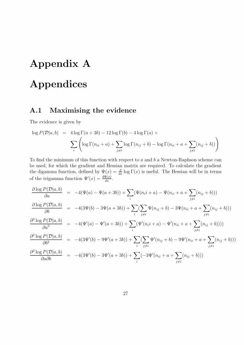
A.1 Maximising the evidence

The evidence is given by

log P (D|a, b) = 4 log Γ(a + 3b) − 12 log Γ(b) − 4 log Γ(a) +

∑

i

(

log Γ(nii + a) +∑

j 6=i

log Γ(nij + b) − log Γ(nii + a +∑

j 6=i

(nij + b))

)

To find the minimum of this function with respect to a and b a Newton-Raphson scheme canbe used, for which the gradient and Hessian matrix are required. To calculate the gradientthe digamma function, defined by Ψ(x) = d

dxlog Γ(x) is useful. The Hessian will be in terms

of the trigamma function Ψ′(x) = dΨ(x)dx

.

∂ log P (D|a, b)

∂a= −4(Ψ(a) − Ψ(a + 3b)) +

∑

i

(Ψ(nii + a) − Ψ(nii + a +∑

j 6=i

(nij + b)))

∂ log P (D|a, b)

∂b= −4(3Ψ(b) − 3Ψ(a + 3b)) +

∑

i

(∑

j 6=i

Ψ(nij + b) − 3Ψ(nii + a +∑

j 6=i

(nij + b)))

∂2 log P (D|a, b)

∂a2 = −4(Ψ′(a) − Ψ′(a + 3b)) +∑

i

(Ψ′(nii + a) − Ψ′(nii + a +∑

j 6=i

(nij + b))))

∂2 log P (D|a, b)

∂b2= −4(3Ψ′(b) − 9Ψ′(a + 3b)) +

∑

i

(∑

j 6=i

Ψ′(nij + b) − 9Ψ′(nii + a +∑

j 6=i

(nij + b)))

∂2 log P (D|a, b)

∂a∂b= −4(3Ψ′(b) − 3Ψ′(a + 3b)) +

∑

i

(−3Ψ′(nii + a +∑

j 6=i

(nij + b)))

27

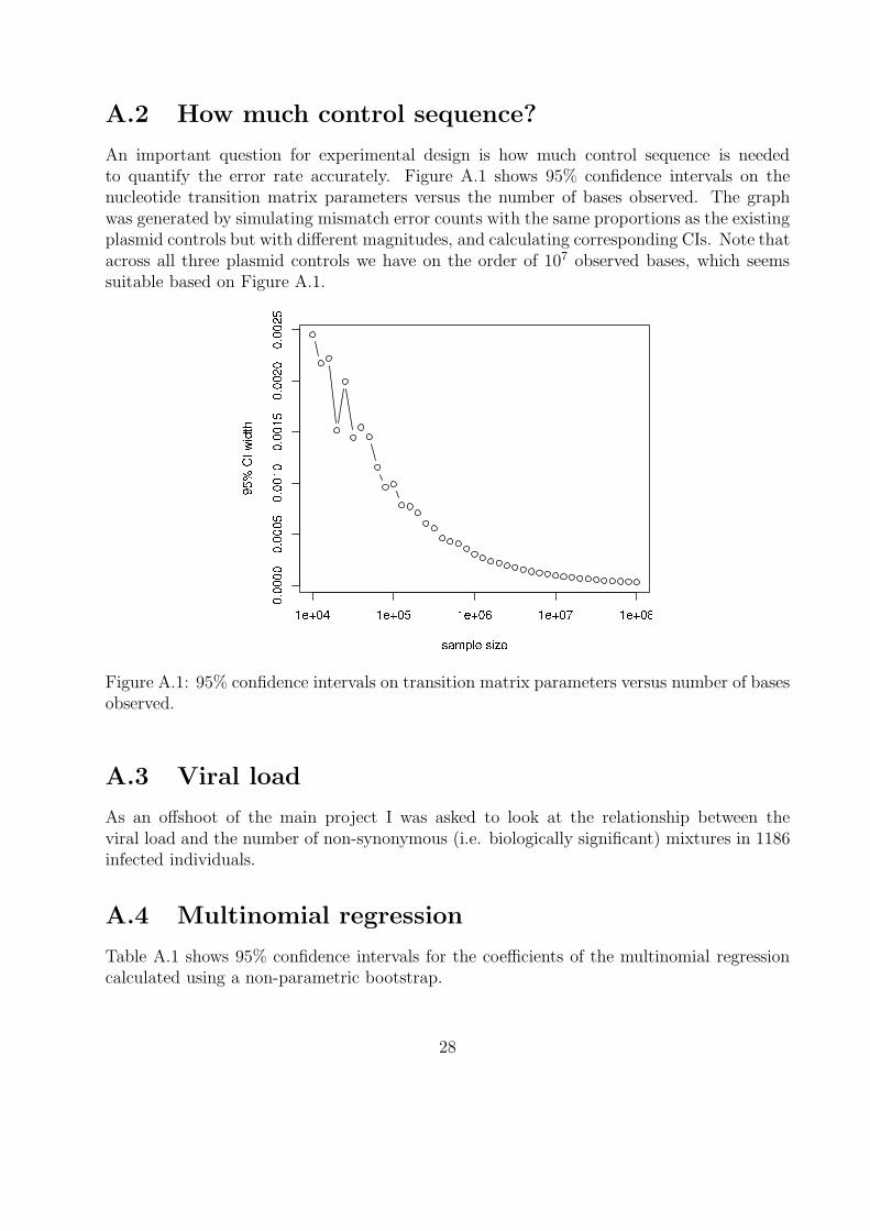
A.2 How much control sequence?

An important question for experimental design is how much control sequence is neededto quantify the error rate accurately. Figure A.1 shows 95% confidence intervals on thenucleotide transition matrix parameters versus the number of bases observed. The graphwas generated by simulating mismatch error counts with the same proportions as the existingplasmid controls but with different magnitudes, and calculating corresponding CIs. Note thatacross all three plasmid controls we have on the order of 107 observed bases, which seemssuitable based on Figure A.1.

Figure A.1: 95% confidence intervals on transition matrix parameters versus number of basesobserved.

A.3 Viral load

As an offshoot of the main project I was asked to look at the relationship between theviral load and the number of non-synonymous (i.e. biologically significant) mixtures in 1186infected individuals.

A.4 Multinomial regression

Table A.1 shows 95% confidence intervals for the coefficients of the multinomial regressioncalculated using a non-parametric bootstrap.

28

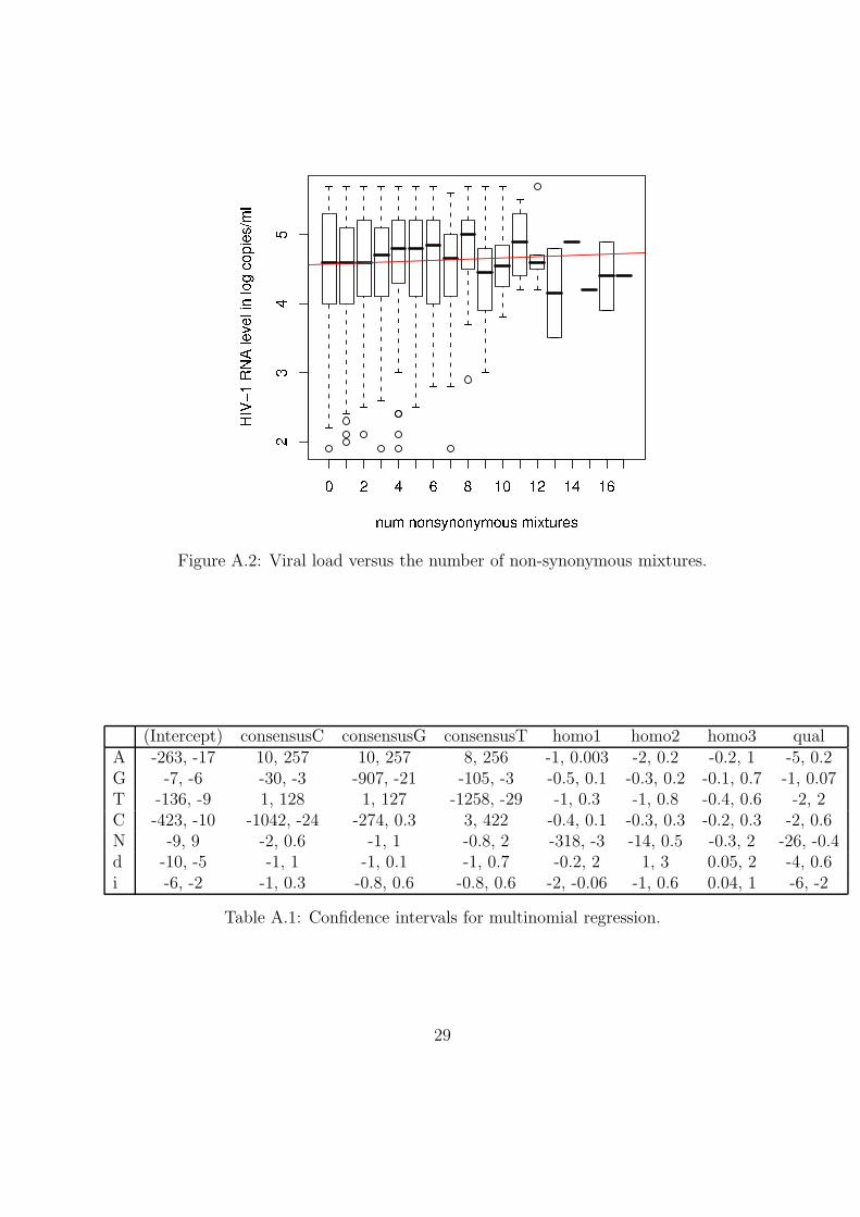
Figure A.2: Viral load versus the number of non-synonymous mixtures.

(Intercept) consensusC consensusG consensusT homo1 homo2 homo3 qualA -263, -17 10, 257 10, 257 8, 256 -1, 0.003 -2, 0.2 -0.2, 1 -5, 0.2G -7, -6 -30, -3 -907, -21 -105, -3 -0.5, 0.1 -0.3, 0.2 -0.1, 0.7 -1, 0.07T -136, -9 1, 128 1, 127 -1258, -29 -1, 0.3 -1, 0.8 -0.4, 0.6 -2, 2C -423, -10 -1042, -24 -274, 0.3 3, 422 -0.4, 0.1 -0.3, 0.3 -0.2, 0.3 -2, 0.6N -9, 9 -2, 0.6 -1, 1 -0.8, 2 -318, -3 -14, 0.5 -0.3, 2 -26, -0.4d -10, -5 -1, 1 -1, 0.1 -1, 0.7 -0.2, 2 1, 3 0.05, 2 -4, 0.6i -6, -2 -1, 0.3 -0.8, 0.6 -0.8, 0.6 -2, -0.06 -1, 0.6 0.04, 1 -6, -2

Table A.1: Confidence intervals for multinomial regression.

29

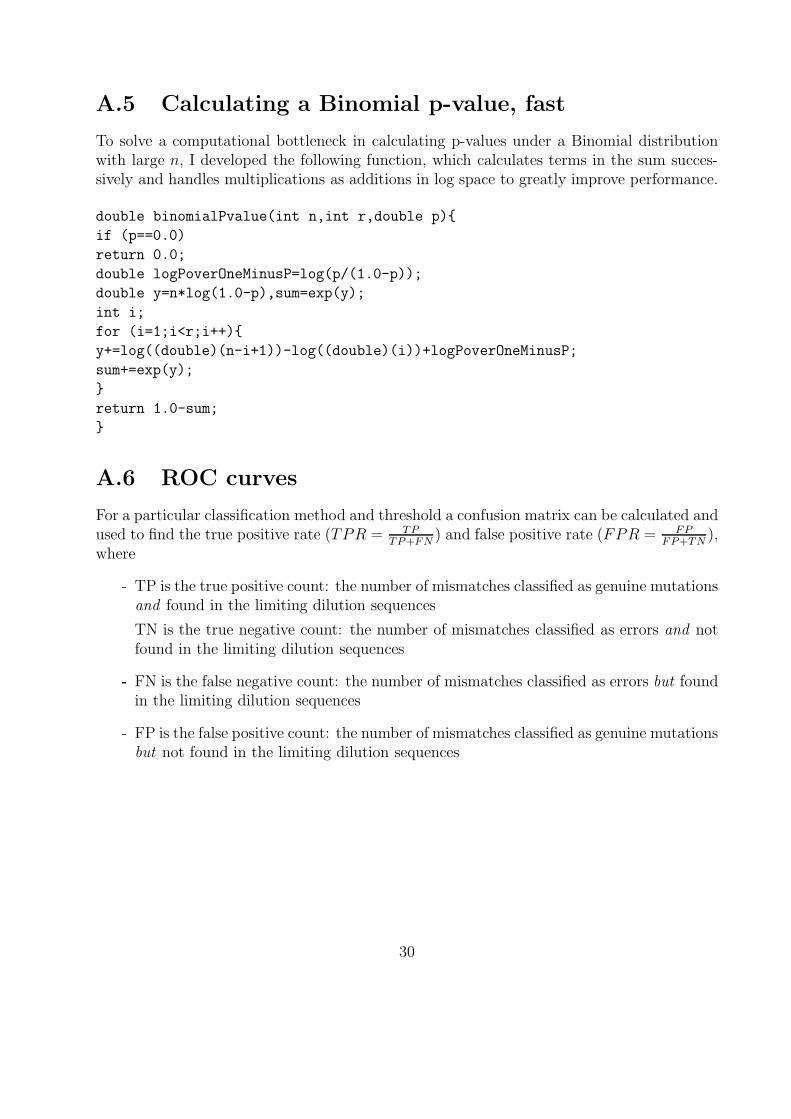
A.5 Calculating a Binomial p-value, fast

To solve a computational bottleneck in calculating p-values under a Binomial distributionwith large n, I developed the following function, which calculates terms in the sum succes-sively and handles multiplications as additions in log space to greatly improve performance.

double binomialPvalue(int n,int r,double p){

if (p==0.0)

return 0.0;

double logPoverOneMinusP=log(p/(1.0-p));

double y=n*log(1.0-p),sum=exp(y);

int i;

for (i=1;i<r;i++){

y+=log((double)(n-i+1))-log((double)(i))+logPoverOneMinusP;

sum+=exp(y);

}

return 1.0-sum;

}

A.6 ROC curves

For a particular classification method and threshold a confusion matrix can be calculated andused to find the true positive rate (TPR = TP

TP+FN) and false positive rate (FPR = FP

FP+TN),

where

- TP is the true positive count: the number of mismatches classified as genuine mutationsand found in the limiting dilution sequences

TN is the true negative count: the number of mismatches classified as errors and notfound in the limiting dilution sequences

-- FN is the false negative count: the number of mismatches classified as errors but foundin the limiting dilution sequences

- FP is the false positive count: the number of mismatches classified as genuine mutationsbut not found in the limiting dilution sequences

30