Statistical timing analysis using bounds and selective …blaauw.engin.umich.edu/wp-content/uploads/sites/342/2017/11/39.pdf · static timing analysis (STA) using so-called case analysis

IEEE TRANSACTIONS ON COMPUTER-AIDED DESIGN OF INTEGRATED CIRCUITS AND SYSTEMS, VOL. 22, NO. 9, SEPTEMBER 2003 1243

Statistical Timing Analysis Using Bounds andSelective Enumeration

Aseem Agarwal, Student Member, IEEE, Vladimir Zolotov, Member, IEEE, and David T. Blaauw, Member, IEEE

Abstract—The growing impact of within-die process variationhas created the need for statistical timing analysis, where gate de-lays are modeled as random variables. Statistical timing analysishas traditionally suffered from exponential run time complexitywith circuit size, due to arrival time dependencies created by re-converging paths in the circuit. In this paper, we propose a new ap-proach to statistical timing analysis which uses statistical boundsand selective enumeration to refine these bounds. First, we providea formal definition of the statistical delay of a circuit and derive astatistical timing analysis method from this definition. Since thismethod for finding the exact statistical delay has exponential runtime complexity with circuit size, we also propose a new methodfor computing statistical bounds which has linear run time com-plexity. We prove the correctness of the proposed bounds. Sincewe provide both a lower and upper bound on the true statisticaldelay, we can determine the quality of the bounds. If the com-puted bounds are not sufficiently close to each other, we propose aheuristic to iteratively improve the bounds using selective enumer-ation of the sample space with additional run time. The proposedmethods were implemented and tested on benchmark circuits. Theresults demonstrate that the proposed bounds have only a smallerror, which can be further reduced using selective enumerationwith modest additional run time.

Index Terms—Probability, process variation, ststistical analysis,yield prediction.

I. INTRODUCTION

STATIC timing analysis has become an indispensable partof performance verification. Traditionally, the variation

in the underlying process parameters have been modeled instatic timing analysis (STA) using so-called case analysis. Inthis methodology, best-case, nominal, and worst-case SPICEparameters sets are constructed and the timing analysis isperformed several times, each time using one case file. Eachexecution of static timing analysis is, therefore, deterministic,meaning that the analysis uses deterministic delays for thegates and any statistical variation in the underlying silicon ishidden. While this approach has been successfully used in thepast to model die-to-die variations in device and interconnectdelay, it is not able to accurately model variations within asingle die. With the continual scaling of feature sizes, theability to control critical device parameters on a single die hasbecome increasingly difficult. Using a worst-case analysis forthese so-calledwithin-die variations, therefore, leads to very

Manuscript received September 24, 2002; revised December 23, 2002. Thispaper was recommended by Associate Editor F. N. Najm.

A. Agarwal and D. T. Blaauw are with the University of Michigan, Ann Arbor,MI 48105 USA (e-mail: [email protected]).

V. Zolotov is with the Motorola, Inc., Austin, TX 78759 USA.Digital Object Identifier 10.1109/TCAD.2003.816217

pessimistic analysis results since it assumes that all devices ona die have worst-case characteristics, ignoring their inherentstatistical variation. The emerging dominance of within-dievariations, therefore, poses a major obstacle for deterministicSTA, giving rise to the need for new statistical timing analysisapproaches.

Variations in the delays of a circuit can be broadly classifiedinto two categories:environmentalvariations andprocessvaria-tions. Environmental variations are caused by uncertainty in theenvironmental conditions during the operation of a chip, suchas power supply and temperature variations. Process variationsare due to uncertainty in the device and interconnect charac-teristics, such as effective gate length, doping concentrations,oxide thickness and ILD thickness. A number of methods havebeen proposed to determine the impact of such variations on thedelay of individual gates and interconnect [13]–[17]. In general,these variations can be divided intobetween-dievariations (orinter- die variation) andwithin-dievariations (or intra-die vari-ations). Within-die variations can have a deterministic compo-nent due to topological dependencies of device processing, suchas CMP effects and topologically correlated lithographic distor-tions [3]–[5]. In some cases, such topological dependencies canbe directly accounted for in the analysis, thereby reducing thestatistical variation [18], [19], whereas in other cases, such vari-ations are treated as random.

In this paper, we propose a formal model and an efficientanalysis method for statistical STA in the presence of randomwithin-die process variations. Since between-die variations areadequately captured using case analysis, we focus on within-dievariations. We also treat all variations as random variations,meaning that topological dependencies are either removed priorto the analysis or are treated as random variations. We alsodo not address environmental variations, although the proposedmodel and analysis methods can be extended to such variations.

Deterministic timing analysis has seen significant improve-ment since it was first introduced [1], [2], including methodsto account for effects such as cross-coupling noise [6]–[11] andpower supply noise [12]. The extensive use of deterministic STAis in large part due to its linear run time complexity with circuitsize. In contrast, statistical STA has an underlying worst-casecomplexity that is exponential with circuit size, which poses afundamental obstacle to its practical application. This high runtime complexity is the result of reconverging paths in the cir-cuit which causes correlations between their path delays due toshared sections of such paths. A second source of correlationbetween arrival times results from spatial and topological cor-relation of the individual gate delays. For instance, gates that arepositioned within close proximity on a die, or that are similar in

0278-0070/03$17.00 © 2003 IEEE

1244 IEEE TRANSACTIONS ON COMPUTER-AIDED DESIGN OF INTEGRATED CIRCUITS AND SYSTEMS, VOL. 22, NO. 9, SEPTEMBER 2003

layout topology, are more likely to have similar gate delays afterfabrication. Due to the correlation between arrival times, manystatistical STA approaches [20]–[27] have either high run timesor they ignore the presence of these correlations. Recently, anumber of new methods have been proposed to address the in-creasing significance of process variations. In [28], [29], a novelmethod using discretized probability distributions is proposed.However, the run time of the method is exponential and the pro-posed approaches to reduce the run time have an unclear impacton the accuracy. In [30], a method using statistical bounds isproposed with gate delays restricted to Gaussian distributions.Since the delay of CMOS gates is nonlinear with respect to itsprocess parameters, the probability distribution of gate delaysis typically not Gaussian. Also, Gaussian distributions are un-bounded, meaning that they predict a finite probability of zerodelay or very large delay for a gate, which is not physically fea-sible. In [31], a path based statistical delay computation is pre-sented which has the advantage that it incorporates an accuratedelay model that accounts for signal slope and output loading.However, the analysis is performed on one path at a time and thenumber of critical and near-critical paths in a circuit can be verylarge, especially in highly optimized circuits. In [32], a new cir-cuit optimization method was, therefore, proposed that reducesthe number of near critical paths in a circuit, thereby improvingthe statistical delay of the circuit. The optimization, however,was performed using deterministic timing analysis.

In this paper, we propose a new method for statistical STA.Since the formulation of statistical STA has varied in subtle butimportant ways in the literature, we first provide a formal modelof statistical STA. We then derive a procedure for statistical STAin a strict manner from this problem formulation. Since the com-putational complexity of this exact statistical STA method is ex-ponential with the circuit size, we also present a new methodfor computing bounds on the exact probability distribution ofthe circuit delay and proof the correctness of these bounds. Thecomputed bounds are themselves probability distribution func-tions that can be used to obtain a conservative estimate of thecircuit delay at any desired confidence point. By restricting ouranalysis to bounds on the true statistical behavior of the circuit,we are able to preserve the important characteristic of determin-istic STA which has a linear run time complexity with circuitsize. Since we provide both a lower and upper bound on thetrue statistical delay, we can determine the quality or error of thecomputed bounds. Finally, we propose a heuristic method to it-eratively improve the computed bounds using selective enumer-ation of the sample space with additional run time. Combined,the proposed methods provide a statistical STA approach withlinear run time, that is guaranteed conservative, has a boundederror, and can be iteratively refined at the expense of additionalcomputational effort. The proposed methods were implementedand tested on benchmark circuits. The difference between theexpected values of the upper and lower bound was shown to besmall, ranging from 2% to 10%, and this difference could bereduced by 62% on average, using the proposed selective enu-meration method, with modest additional run time.

The remainder of this paper is organized as follows. In Sec-tion II, we present a formal model of statistical STA and ourmodeling assumptions. In Section III, we present a number of

probabilistic timing graph transformations. In Section IV, wederive our method for exact statistical timing analysis. In Sec-tion V, we present the computation of the lower and upper sta-tistical bounds on the true statistical behavior. In Section VI,we present methods for exact graph reduction and for refine-ment of the computed bounds using selective enumeration. InSection VII, we present our results and in Section VIII our con-cluding remarks.

II. STATISTICAL TIMING ANALYSIS FORMULATION

In this section, we present a formal model of statistical statictiming analysis. Our goal is to model the impact of gate delayvariations due to within-die process variations on the circuitdelay. Although at design time, the delay of each gate is un-known, after a chip has been manufactured, the gate delays arefixed and have a deterministic value for each particular die. Thefabrication of a large set of die can be thought of as our proba-bilistic experiment, and each fabricated die as an experimentaloutcome. The randomness or variability of the circuit delay is,therefore, over the fabricated die, and it is the probability distri-bution of the circuit delay that statistical timing analysis aims toobtain.

At this point, we do not account for temporal variations ofthe gate delays due to environmental factors, such as powersupply fluctuations, temperature dependence and noise, whichare better modeled using case analysis. However, our generalanalysis approach could be extended to these types of variationsas well. Also, for simplicity of formulation, we ignore the pres-ence of false paths since these are orthogonal to the issues dis-cussed in this paper. We now give the following definition of atiming graph:

Definition 1: A timing graph is a directed graph having ex-actly one source and one sink node: , where

is a set of nodes,is a set of edges, is the source node, and isthe sink node and each edge is simply an ordered pair ofnodes .

The nodes in the timing graph correspond to nets in the cir-cuit, and the edges in the graph correspond to connections fromgate inputs to gate outputs. Although circuits generally havemultiple inputs and outputs, we can trivially transform them tographs with a single source and sink by adding a virtual sourceand sink node.

In our formulation, adeterministictiming graph repre-sents a particular manufactured die, where each gate has a fixeddelay value. Each edgein is assigned a delay , whichrepresents the deterministic propagation delay from a gate’sinput to its output. Similar to other statistical STA methods, weignore the dependence of gate delay on the transition time of thegate input signals.

A path of a timing graph is a sequence of nodes, suchthat each pair of adjacent nodes and has an edge

. The path delay of path is the sum of all the delaysof edges on path . Among all paths terminating at

a node , we define the path with the maximum delay as thecritical path of . The delay of the critical path terminating at anode is equal to itsarrival time, . The critical path of the

AGARWAL et al.: STATISTICAL TIMING ANALYSIS USING BOUNDS AND SELECTIVE ENUMERATION 1245

Fig. 1. Delay probability density and cumulative distribution functions.

sink node of a timing graph is referred to asthecritical pathof the timing graph, and the arrival time of , is referred to asits graph delay.

After fabrication, a deterministic timing graph can beconceptually formulated for each die. However, during the de-sign of a chip, the gate delays are unknown and must be modeledas random variables. Each gate delay is, therefore, specified ei-ther with a cumulative probability distribution function (CDF)or probability density function (pdf) and we define aproba-bilistic timing graph as follows.

Definition 2: A probabilistic timing graph is a timinggraph whose edges are assigned random variables of delayvalues.

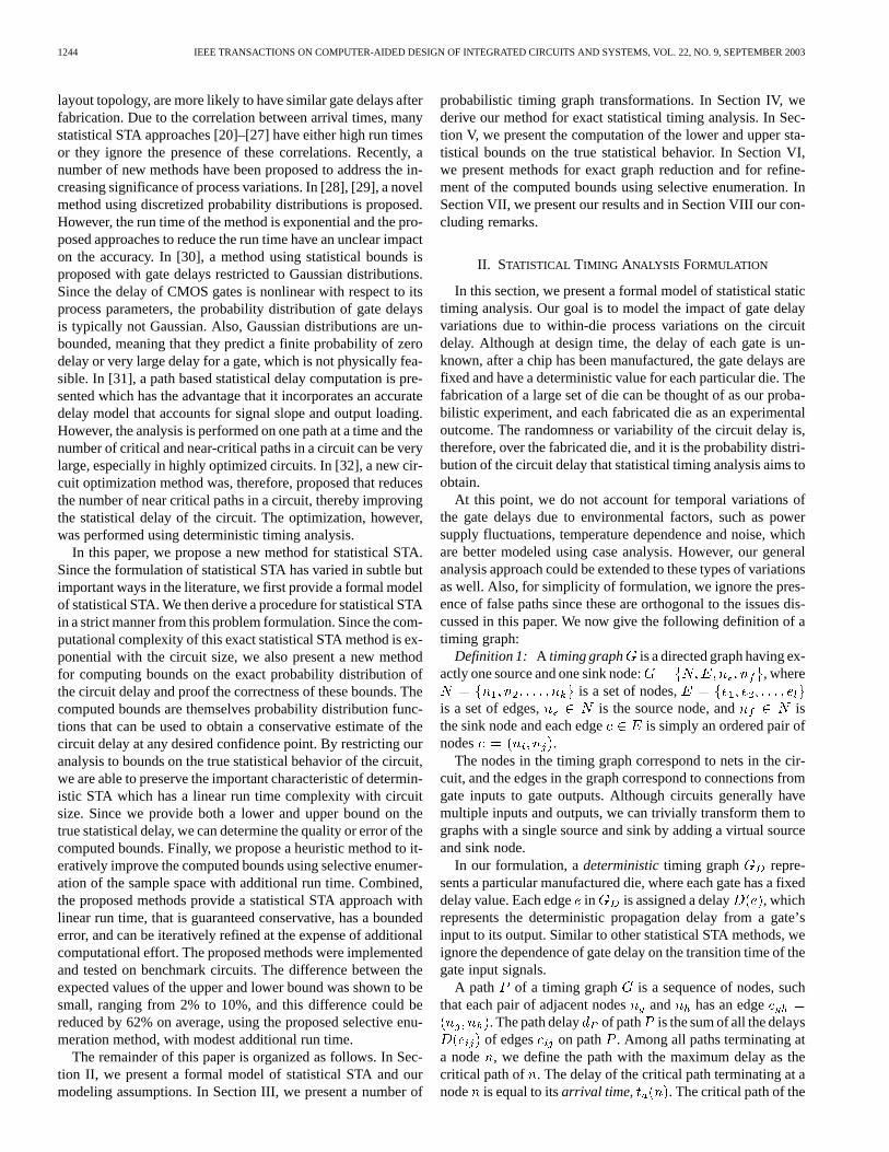
Fig. 1 shows an example of a delay cumulative probabilitydistribution function and its corresponding probability densityfunction. Since these functions represent the variation of gatedelays, they have the following obvious but important property:

Property 1: A delay CDF equals 0 for all delay values lessthan a finite minimum value and equals 1 for all valuesgreater than a finite maximum value . A delay pdf isnonzero only on a finite interval [ ].

These properties follow from the fact that the delay of a realgate cannot be less that some finite minimum delay valueor more than some finite maximum delay value .

We assume statistical independence of all edge delays, similarto a number of previous statistical STA methods [20]–[25], [28],[29], [31]. In practice, edge delays may be spatially or topolog-ically correlated, meaning that gates located within close prox-imity of each other or that have similar layout topologies willhave an increased likelihood of having similar gate delays. Thespatial and topological correlations between gate delays impactsthe distribution of the circuit delay and complicates the anal-ysis by creating additional correlations between path delays.We explicitly state the assumed independence of gate delay in anumber of places and also note here that the entire formulationpresented in this paper is based on this assumption. The con-tribution of this paper is, therefore, that it provides an efficientsolution to the problem of path delay correlation due to path re-convergence. However, the methods presented in this paper canalso be extended to timing graphs with correlated edge delays.Note also that our method does not restrict the shape of the CDFof edge delays to some specific shape, such as a Gaussian dis-tribution. The shape of the edge delay CDFs are unrestricted aslong as they satisfy Property 1 and they are valid probability dis-tribution functions.

To simplify the implementation of statistical STA, it is oftenmore convenient to approximate continuous probability densityand cumulative distribution functions with discrete functions. Adiscrete pdf, corresponding to continuous pdf , can be rep-resented by a sequence of pairs ( ), where and

. For computational efficiency, we usediscrete pdfs and CDFs in the final implementation of our pro-posed statistical timing analysis approach. However, for gener-ality, we will formulate the statistical timing analysis task usingcontinuous functions.

We now consider the sample spaceof a probabilistic timinggraph , consisting of all deterministic timing graphs withedge delays corresponding to the nonzero values of their proba-bility distribution functions. The probability that a timing graph

in has edges with delay between and is

(1)

where is the joint probability density func-tion of edge delays. Since, as previously stated, we assumethat all edge delays are independent random variables, this jointprobability function is simply the product of the individual prob-ability density functions of edge delaysand we can rewrite (1)as follows [35]:

(2)

where is the delay probability density function of edge.Given a deterministic timing graph in , we can compute

its delay , using any of the currently available means,such as traditional static timing analysis. The delay is,therefore, defined on the sample spaceand is a random vari-able. The objective of statistical timing analysis is to find theCDF of , which is defined as follows.

Definition 3: The cumulative probability distribution func-tion of the delay of a probabilistic timing graph with indepen-dent edge delays is expressed as

(3)


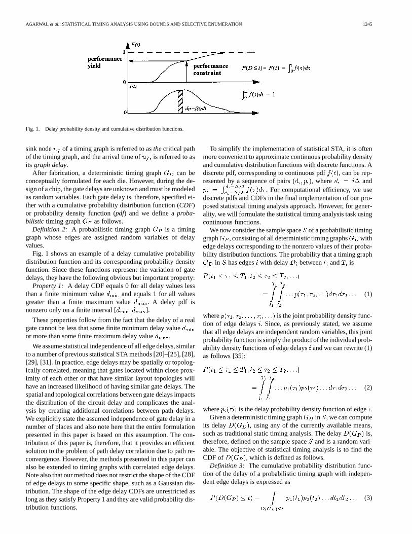
Fig. 2. Graph representation of gates with correlated pin-to-pin delays and interconnect delay variations.

where is the probability density function of the delayof edge and the integration is performed over the volume ofsample space where the delay of timing graph isless than .

The probability density function can be computed by simpledifferentiation of the CDF. The cumulative probability distri-bution function of the graph delay can be used in a number ofways. First, given a particular performance constraint, the prob-ability of obtaining a fabricated die that meets or exceeds thisconstraint can be determined, as illustrated in Fig. 1. The prob-ability of obtaining a die that meets the specified performanceis also referred to as theperformance yield. A design, for in-stance, can be improved until its performance yield meets a suf-ficient level. The graph delay CDF is also useful to determinethe number of expected dies in a certain performance range, al-lowing prediction of the performance “binning” of the design.Conversely, given a required performance yield, the expectedperformance can be obtained. This allows a designer to deter-mine, for instance, the minimum expected performance of 95%of the fabricated dies.

If we use discrete edge delay pdfs, we can compute the graphdelay pdf by enumerating the entire sample space consistingof all combinations of the nonzero delay probabilities of alledges. For each enumerated timing graph in the samplespace, we can then compute the graph delay and its probabilityof occurrence. By summing the probability of all samples withsame delay, we then obtain the probability density function ofthe graph delay, shown in Fig. 1(b). Of course, this method isexponential in its run time complexity with circuit size and isnot useful as a practical solution. However, its formulation isuseful as a formal definition and for understanding the under-lying problem that needs to be solved.

Finally, we note that each edge in the timing graph is associ-ated with a so-calledpin-to-pindelay from an input node of agate to the output node of that gate. An-input gate is, therefore,represented with edges in the timing graph. Since all edgedelays are independent, this assumes that all pin-to-pin delaysof a gate are independent. In practice, the pin-to-pin delays ofa gate will be strongly correlated since they are determined bycommon transistors in the gate structure. To address this correla-tion, the graph representation of a gate can be extended to modelthis dependence using the representation as shown in Fig. 2(a).Each gate is represented with a set of fanin edgesin series

(a)

(b)

Fig. 3. Series and parallel reduction.

with a single fanout edge . The total pin-to-pin delay ofthe gate is then distributed among edgesand , wherethe delays of represent the uncorrelated component of thepin-to-pin delays and represents the correlated componentof the pin-to-pin delay. Note that this model can be extendedto include interconnect delay, as shown in Fig. 2(b), with addi-tional edges representing the delay from the gate output node tothe sink nodes of the interconnect.

III. PROBABILISTIC TIMING GRAPH TRANSFORMS

Before we discuss exact and bounded methods for com-puting the CDF of the graph delay, we briefly discuss threebasic transformations for probabilistic timing graphs withindependent edge delays.

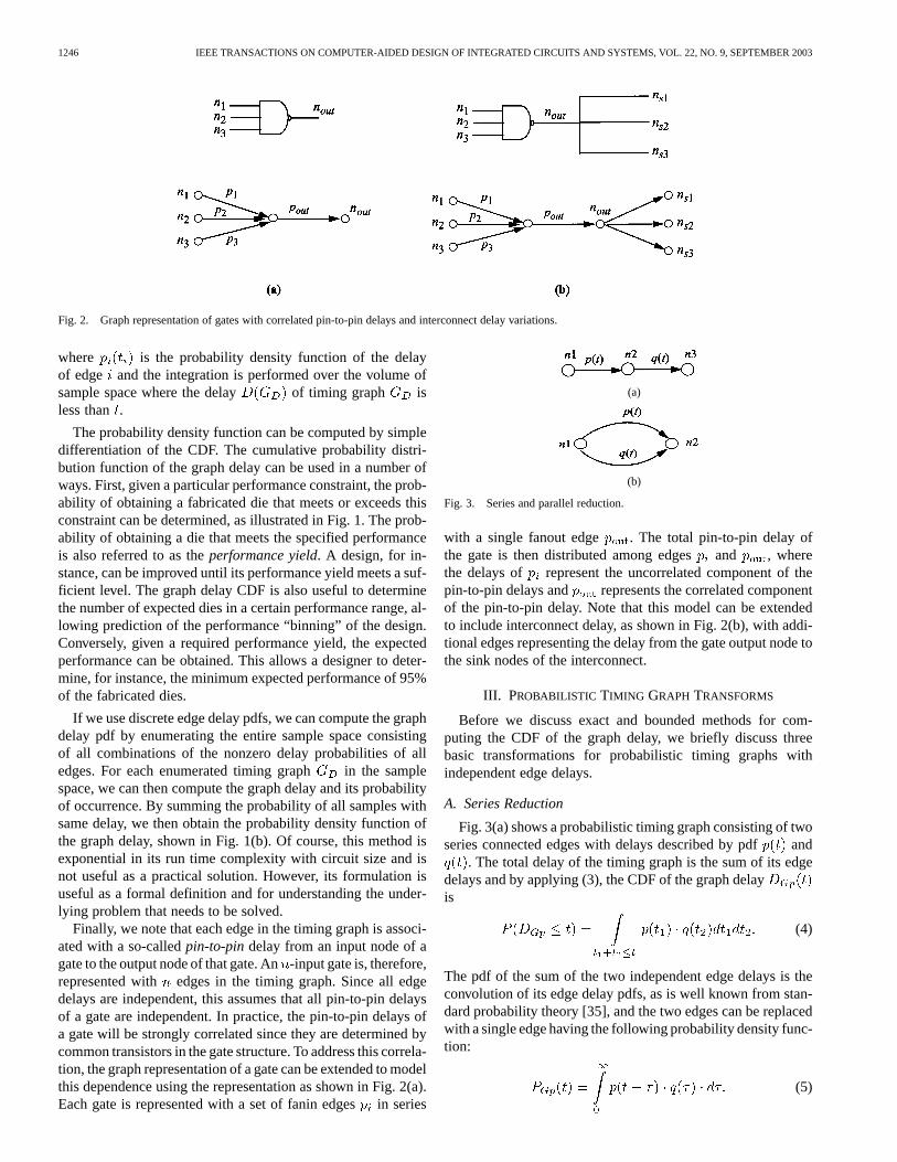
A. Series Reduction

Fig. 3(a) shows a probabilistic timing graph consisting of twoseries connected edges with delays described by pdfand

. The total delay of the timing graph is the sum of its edgedelays and by applying (3), the CDF of the graph delayis

(4)

The pdf of the sum of the two independent edge delays is theconvolution of its edge delay pdfs, as is well known from stan-dard probability theory [35], and the two edges can be replacedwith a single edge having the following probability density func-tion:

(5)


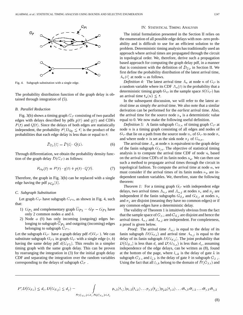
Fig. 4. Subgraph substitution with a single edge.

The probability distribution function of the graph delay is ob-tained through integration of (5).

B. Parallel Reduction

Fig. 3(b) shows a timing graph consisting of two paralleledges with delays described by pdfs and and CDFs

and . Since the delays of both edges are statisticallyindependent, the probability is the product of theprobabilities that each edge delay is less than or equal to:

(6)

Through differentiation, we obtain the probability density func-tion of the graph delay as follows:

(7)

Therefore, the graph in Fig. 3(b) can be replaced with a singleedge having the pdf .

C. Subgraph Substitution

Let graph have subgraph , as shown in Fig. 4, suchthat:

1) and complementary graph haveonly 2 common nodes and .

2) Node ( ) has only incoming (outgoing) edges be-longing to subgraph and outgoing (incoming) edgesbelonging to subgraph .

Let the subgraph have a graph delay pdf . We cansubstitute subgraph in graph with a single edge ( )having the same delay pdf . This results in a simplertiming graph with the same graph delay. This can be provenby rearranging the integration in (3) for the initial graph delayCDF and separating the integration over the random variablescorresponding to the delays of subgraph .

IV. STATISTICAL TIMING ANALYSIS

The initial formulation presented in the Section II relies onthe enumeration of all possible edge delays with nonzero prob-ability and is difficult to use for an efficient solution to theproblem. Deterministic timing analysis has traditionally used anapproach where arrival times are propagated through the circuitin topological order. We, therefore, derive such a propagationbased approach for computing the graph delay pdf, in a mannerthat is consistent with the definition of in Section II. Wefirst define the probability distribution of the latest arrival time,

at node as follows.Definition 4: The latest arrival time at node of is

a random variable where its CDF is the probability that adeterministic timing graph in the sample space hasan arrival time .

In the subsequent discussion, we will refer to the latest ar-rival time as simplythearrival time. We also note that a similarderivation can be performed for theearliestarrival time. Also,the arrival time for the source node is a deterministic valueequal to 0. We now make the following useful definition.

Definition 5: A fanin subgraph of timing graph atnode is a timing graph consisting of all edges and nodes of

that lie on a path from the source nodeof to node ,and where node is set as the sink node of .

The arrival time at node is equivalent to the graph delayof the fanin subgraph . The objective of statistical timinganalysis is to compute the arrival time CDF of node, basedon the arrival time CDFs of its fanin nodes. We can then usesuch a method to propagate arrival times through the circuit intopological fashion. To compute the arrival time at node, wemust consider if the arrival times of its fanin nodesare in-dependent random variables. We, therefore, state the followingtheorem:

Theorem 1: For a timing graph with independent edgedelays, two arrival times and at nodes and areindependent if the fanin subgraphs and at nodesand are disjoint (meaning they have no common edges) or ifany common edges have a deterministic delay.

The validity of Theorem 1 is intuitively obvious from the factthat the sample space of and are disjoint and hence thearrival times and are independent. For completeness,a proof is given below.

Proof: The arrival time is equal to the delay of itsfanin subgraph and arrival time is equal to thedelay of its fanin subgraph . The joint probability that

is less than and is less than , assumingindependence of the edge delays, can be written as (8), foundat the bottom of the page, where is the delay of gate insubgraph and is the delay of gate in subgraph .Using the fact that all belong to the domain of and

(8)


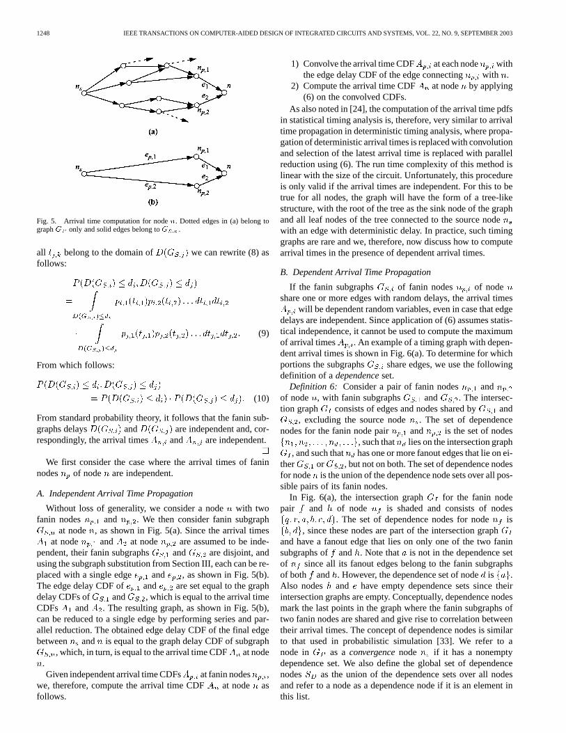
Fig. 5. Arrival time computation for noden. Dotted edges in (a) belong tographG only and solid edges belong toG .

all belong to the domain of we can rewrite (8) asfollows:

(9)

From which follows:

(10)

From standard probability theory, it follows that the fanin sub-graphs delays and are independent and, cor-respondingly, the arrival times and are independent.

We first consider the case where the arrival times of faninnodes of node are independent.

A. Independent Arrival Time Propagation

Without loss of generality, we consider a nodewith twofanin nodes and . We then consider fanin subgraph

at node , as shown in Fig. 5(a). Since the arrival timesat node and at node are assumed to be inde-

pendent, their fanin subgraphs and are disjoint, andusing the subgraph substitution from Section III, each can be re-placed with a single edge and , as shown in Fig. 5(b).The edge delay CDF of and are set equal to the graphdelay CDFs of and , which is equal to the arrival timeCDFs and . The resulting graph, as shown in Fig. 5(b),can be reduced to a single edge by performing series and par-allel reduction. The obtained edge delay CDF of the final edgebetween and is equal to the graph delay CDF of subgraph

, which, in turn, is equal to the arrival time CDF at node.Given independent arrival time CDFs at fanin nodes ,

we, therefore, compute the arrival time CDF at node asfollows.

1) Convolve the arrival time CDF at each node withthe edge delay CDF of the edge connecting with .

2) Compute the arrival time CDF at node by applying(6) on the convolved CDFs.

As also noted in [24], the computation of the arrival time pdfsin statistical timing analysis is, therefore, very similar to arrivaltime propagation in deterministic timing analysis, where propa-gation of deterministic arrival times is replaced with convolutionand selection of the latest arrival time is replaced with parallelreduction using (6). The run time complexity of this method islinear with the size of the circuit. Unfortunately, this procedureis only valid if the arrival times are independent. For this to betrue for all nodes, the graph will have the form of a tree-likestructure, with the root of the tree as the sink node of the graphand all leaf nodes of the tree connected to the source nodewith an edge with deterministic delay. In practice, such timinggraphs are rare and we, therefore, now discuss how to computearrival times in the presence of dependent arrival times.

B. Dependent Arrival Time Propagation

If the fanin subgraphs of fanin nodes of nodeshare one or more edges with random delays, the arrival times

will be dependent random variables, even in case that edgedelays are independent. Since application of (6) assumes statis-tical independence, it cannot be used to compute the maximumof arrival times . An example of a timing graph with depen-dent arrival times is shown in Fig. 6(a). To determine for whichportions the subgraphs share edges, we use the followingdefinition of adependenceset.

Definition 6: Consider a pair of fanin nodes andof node , with fanin subgraphs and . The intersec-tion graph consists of edges and nodes shared by and

, excluding the source node . The set of dependencenodes for the fanin node pair and is the set of nodes

, such that lies on the intersection graph, and such that has one or more fanout edges that lie on ei-

ther or , but not on both. The set of dependence nodesfor node is the union of the dependence node sets over all pos-sible pairs of its fanin nodes.

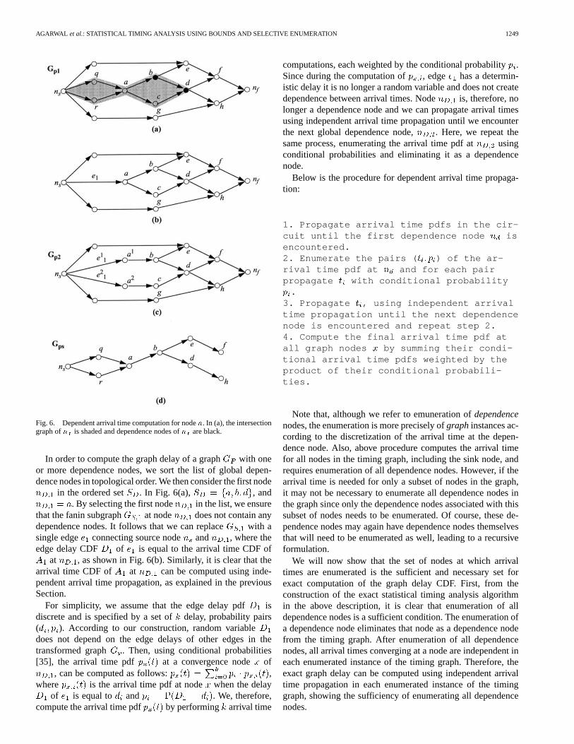
In Fig. 6(a), the intersection graph for the fanin nodepair and of node is shaded and consists of nodes

. The set of dependence nodes for nodeis, since these nodes are part of the intersection graph

and have a fanout edge that lies on only one of the two faninsubgraphs of and . Note that is not in the dependence setof since all its fanout edges belong to the fanin subgraphsof both and . However, the dependence set of nodeis .Also nodes and have empty dependence sets since theirintersection graphs are empty. Conceptually, dependence nodesmark the last points in the graph where the fanin subgraphs oftwo fanin nodes are shared and give rise to correlation betweentheir arrival times. The concept of dependence nodes is similarto that used in probabilistic simulation [33]. We refer to anode in as aconvergencenode if it has a nonemptydependence set. We also define the global set of dependencenodes as the union of the dependence sets over all nodesand refer to a node as a dependence node if it is an element inthis list.


Fig. 6. Dependent arrival time computation for noden. In (a), the intersectiongraph ofn is shaded and dependence nodes ofn are black.

In order to compute the graph delay of a graph with oneor more dependence nodes, we sort the list of global depen-dence nodes in topological order. We then consider the first node

in the ordered set . In Fig. 6(a), , and. By selecting the first node in the list, we ensure

that the fanin subgraph at node does not contain anydependence nodes. It follows that we can replace with asingle edge connecting source node and , where theedge delay CDF of is equal to the arrival time CDF of

at , as shown in Fig. 6(b). Similarly, it is clear that thearrival time CDF of at can be computed using inde-pendent arrival time propagation, as explained in the previousSection.

For simplicity, we assume that the edge delay pdf isdiscrete and is specified by a set ofdelay, probability pairs( ). According to our construction, random variabledoes not depend on the edge delays of other edges in thetransformed graph . Then, using conditional probabilities[35], the arrival time pdf at a convergence node of

, can be computed as follows: ,where is the arrival time pdf at node when the delay

of is equal to and . We, therefore,compute the arrival time pdf by performing arrival time

computations, each weighted by the conditional probability.Since during the computation of , edge has a determin-istic delay it is no longer a random variable and does not createdependence between arrival times. Node is, therefore, nolonger a dependence node and we can propagate arrival timesusing independent arrival time propagation until we encounterthe next global dependence node, . Here, we repeat thesame process, enumerating the arrival time pdf at usingconditional probabilities and eliminating it as a dependencenode.

Below is the procedure for dependent arrival time propaga-tion:

1. Propagate arrival time pdfs in the cir-cuit until the first dependence node isencountered.2. Enumerate the pairs ( ) of the ar-rival time pdf at and for each pairpropagate with conditional probability

.3. Propagate , using independent arrivaltime propagation until the next dependencenode is encountered and repeat step 2.4. Compute the final arrival time pdf atall graph nodes by summing their condi-tional arrival time pdfs weighted by theproduct of their conditional probabili-ties.

Note that, although we refer to emuneration ofdependencenodes, the enumeration is more precisely ofgraphinstances ac-cording to the discretization of the arrival time at the depen-dence node. Also, above procedure computes the arrival timefor all nodes in the timing graph, including the sink node, andrequires enumeration of all dependence nodes. However, if thearrival time is needed for only a subset of nodes in the graph,it may not be necessary to enumerate all dependence nodes inthe graph since only the dependence nodes associated with thissubset of nodes needs to be enumerated. Of course, these de-pendence nodes may again have dependence nodes themselvesthat will need to be enumerated as well, leading to a recursiveformulation.

We will now show that the set of nodes at which arrivaltimes are enumerated is the sufficient and necessary set forexact computation of the graph delay CDF. First, from theconstruction of the exact statistical timing analysis algorithmin the above description, it is clear that enumeration of alldependence nodes is a sufficient condition. The enumeration ofa dependence node eliminates that node as a dependence nodefrom the timing graph. After enumeration of all dependencenodes, all arrival times converging at a node are independent ineach enumerated instance of the timing graph. Therefore, theexact graph delay can be computed using independent arrivaltime propagation in each enumerated instance of the timinggraph, showing the sufficiency of enumerating all dependencenodes.


Next, we show that enumeration of all dependence nodes isalso a necessary condition, meaning that it is not possible toenumerate fewer nodes without arrival time dependencies re-maining in the circuit. Without loss of generality, we considerconvergence node in Fig. 6(a) with fanin nodes and andwith dependence nodes . We now show how, based on theproperties of dependence nodes given in Definition 6, enumer-ation of node is necessary. Since we only use properties spec-ified in Definition 6, the same arguments also translate to node

and all other dependence nodes in a circuit. We first observethat there exists a path from nodeto both node and since,based on Definition 6, nodelies on the intersection of the faninsubgraphs of nodesand . Also, based on Definition 6, at leastone fanout edge of does not lie on both fanin subgraphs, butonly on one of the fanin subgraphs. In Fig. 6(a) this is edge ()which lies on the fanin subgraph ofbut not the fanin subgraphof . From this, it follows that there exists at least one pair ofpaths ( ) from node to nodes and , such that this pair ofpaths is disjoint, meaning they do not share any common edges.In Fig. 6(a), this pair of paths is and .

We now consider subgraph of timing graph , con-sisting of all edges and nodes on pathsand and on faninsubgraph of , as shown in Fig. 6(d). We assume that nodesand have arrival times and , respectively. We now showthat enumeration of nodeis a necessary condition to ensurethat arrival times and are independent. First, we note thatenumeration of any nodes in the fanin subgraph of(consistingof nodes , , and ) does not eliminate the dependence between

and , since the fanin edge ( ) of node will still con-tribute a common, random delay to both and . Second,enumeration of any nodes that lie only on either pathor(such as nodesand ) also does not eliminate the dependencebetween and since these nodes affect only one of the twopaths. Therefore, since enumeration of any node other that node

in subgraph does not eliminate the dependence ofand, it follows that enumeration of nodeis a necessary condi-

tion for eliminating this dependence.In the original timing graph , the arrival times propagated

along and combine with arrival times from other paths.However, it is clear that the dependence between arrival timespropagated along and is sufficient to create dependencebetween the arrival times at nodesand in , even after thearrival times along and combine with other arrival times.From this it follows that enumeration of dependence nodeis anecessary condition for eliminating the dependence between thearrival times at node and in . Since node was chosenas a generic dependence node and we only relied on its proper-ties as defined by Definition 6, the same arguments apply to alldependence nodes and it follows that enumeration of all depen-dence nodes is a necessary condition for exact statistical timinganalysis using independent arrival time propagation.

The number of dependence nodes is typically significantlyless then the number of edges in . Dependent arrival timepropagation, therefore, has a lower complexity than enumera-tion of the entire sample space. Nevertheless, the run time re-mains exponentially with the number of dependence nodes dueto the recursive formulation of the method. Dependent arrivaltime propagation is, therefore, useful only for very small timing

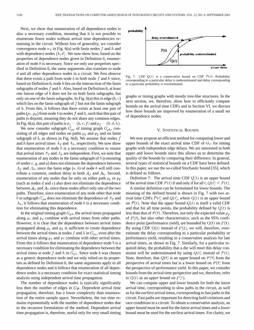
Fig. 7. CDF Q(t) is a conservative bound on CDFP (t). Probabilitycorresponding to a particular delay is underestimated and delay correspondingto a particular probability is overestimated.

graphs or timing graphs with mostly tree-like structures. In thenext section, we, therefore, show how to efficiently computebounds on the arrival time CDFs and in Section VI, we discusshow these bounds are improved by enumeration of a small setof dependence nodes.

V. STATISTICAL BOUNDS

We now propose an efficient method for computing lower andupper bounds of the exact arrival time CDF of for timinggraphs with independent edge delays. We are interested in bothupper and lower bounds since this allows us to determine thequality of the bounds by comparing their difference. In general,several types of statistical bounds on a CDF have been defined.In this paper, we use the so-called Stochastic bound [35], whichis defined as follows.

Definition 7: The arrival time CDF is an upper boundof the arrival time CDF if and only if for all , .

A similar definition can be formulated for lower bounds. Themeaning of the defined bound is shown in Fig. 7 with two ar-rival time CDFs and , where is an upper boundon . Note that the upper bound is itself a valid CDFand that for all time points, the probability defined by isless than that of . Therefore, not only the expected valueof , but also other characteristics, such as the 95% confi-dence point (performance yield), are bounded by on .By using CDF instead of , we will, therefore, over-estimate the delay corresponding to a particular probability orperformance yield, resulting in a conservative analysis for latearrival times, as shown in Fig. 7. Similarly, for a particular re-quired delay, the probability that a die will meet this delay con-straint will be underestimated by using instead of .Note, therefore, that is an upper bound on from theperspective of arrival times but is a lower bound on fromthe perspective of performance yield. In this paper, we considerbounds from the arrival time perspective and we, therefore, referto as anupperbound on .

We can compute upper and lower bounds for both thelatestarrival time, corresponding to slow paths in the circuit, as wellas for theearliestarrival times, corresponding to fast paths in thecircuit. Fast paths are important for detecting hold violations andrace conditions in a circuit. To obtain a conservative analysis, anupperbound must be used for thelatestarrival times and alowerbound must be used for theearliestarrival times. For clarity, we


focus in this paper on late arrival times, although the analysiscan be applied to early arrival times as well.

A. Upper Bound Computation

To efficiently compute an upper bound on the exact graphdelay CDF of , we propose the following theorem for randomvariables.

Theorem 2: Let , and be independent random variablesthat satisfy Property 1. Let , be independent random vari-ables with CDFs that are identical to the CDF of, and that arealso independent from and . The CDF of random variable

is an upper bound on the CDF of randomvariable .

Proof: The probability distribution function of randomvariables and are

(11)

(12)

where , , are the probability density functions of, and , respectively. Multiplying (11) by the integral of prob-

ability density function , rearranging some ofthe terms and renaming integration variables, gives us:

(13)Integrals from formulae (12) and (13) for probabilitydistributions and have the same integrationfunctions and

and differ only in thenames of the variables. Note that random variableis inde-pendent from random variables, and . We now split the4D domain of both functions into two subdomains:and . Probability distributions and can berepresented as the sum of two terms corresponding to thecontribution of each subdomain:

(14)

(15)

Fig. 8. Bounded graph transformation through node splitting.

For subdomain we define a one to one mapping (bijec-tion) so that ( ) corresponds to ( ) i.e.,and . In this subdomain and therefore, inequality

follows from inequality. Therefore, the region of integra-

tion for computing includes the integration region forcomputing and hence because inboth cases we integrate the same function .

For subdomain we define a one to one mapping (bijec-tion) so that ( ) corresponds to ( ) i.e.,and . Similar to the above consideration,

follows fromin this subdomain and the region of inte-

gration for computing includes the region of integrationfor computing . Therefore, .

Combining inequalities for and from each sub-domain, we obtain the inequality for the wholesample space, which proves the theorem.

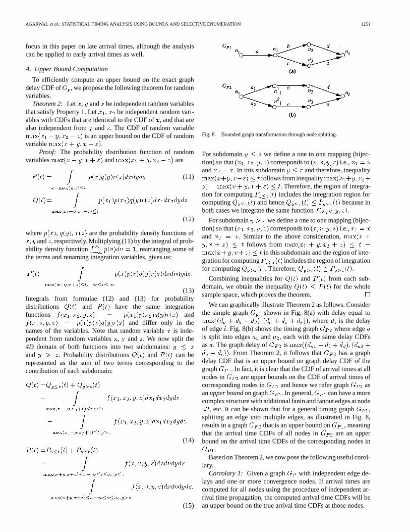
We can graphically illustrate Theorem 2 as follows. Considerthe simple graph shown in Fig. 8(a) with delay equal to

, where is the delayof edge . Fig. 8(b) shows the timing graph where edgeis split into edges and , each with the same delay CDFsas . The graph delay of is

. From Theorem 2, it follows that has a graphdelay CDF that is an upper bound on graph delay CDF of thegraph . In fact, it is clear that the CDF of arrival times at allnodes in are upper bounds on the CDF of arrival times ofcorresponding nodes in and hence we refer graph asanupper boundon graph . In general, can have a morecomplex structure with additional fanin and fanout edges at node

, etc. It can be shown that for a general timing graph ,splitting an edge into multiple edges, as illustrated in Fig. 8,results in a graph that is an upper bound on , meaningthat the arrival time CDFs of all nodes in are an upperbound on the arrival time CDFs of the corresponding nodes in

.Based on Theorem 2, we now pose the following useful corol-

lary.Corrolary 1: Given a graph with independent edge de-

lays and one or more convergence nodes. If arrival times arecomputed for all nodes using the procedure of independent ar-rival time propagation, the computed arrival time CDFs will bean upper bound on the true arrival time CDFs at those nodes.


Fig. 9. Lower bound computation for two dependent arrival times.

The validity of Corrolary 1 can be seen by considering thetiming graph with dependence node, as illustrated inFig. 6(a). Following the procedure for dependent arrival timepropagation, we replace subgraph with a single edge ,as shown in Fig. 6(b), where the edge delay CDF ofis equalto the arrival time CDF at . We now create a graph , asshown in Fig. 6(c), which bounds by splitting edge , suchthat is no longer a dependence node in . By repeatingthis process for all dependence nodes, we obtain a timing graph

that bounds the original timing graph and which hasno dependence nodes. We can compute the exact arrival timeCDF of by performing independent arrival time propaga-tion. Finally, it is easy to observe that we need not explicitlyreplace subgraph with edge and subsequently split it.Instead, we will compute identical arrival times to those ofby simply performing independent arrival time propagation ongraph , as stated in Corrolary 1.

This leads to the useful observation that an upper bound onthe arrival times of a timing graph is obtained by ignoring thedependencies of arrival times and simply applying the procedurefor independent arrival time computation, which has a linear runtime complexity with circuit size.

B. Lower Bound Computation

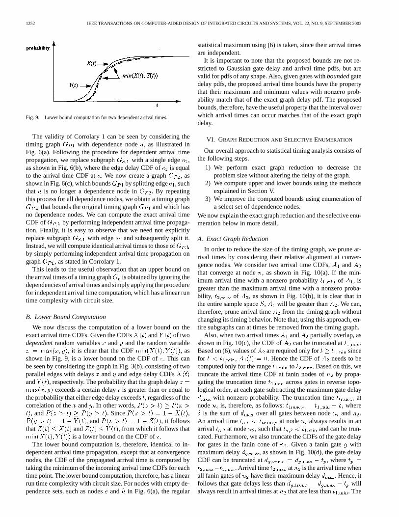
We now discuss the computation of a lower bound on theexact arrival time CDFs. Given the CDFs and of twodependentrandom variables and and the random variable

, it is clear that the CDF , asshown in Fig. 9, is a lower bound on the CDF of. This canbe seen by considering the graph in Fig. 3(b), consisting of twoparallel edges with delays and and edge delay CDFsand , respectively. The probability that the graph delay

exceeds a certain delayis greater than or equal tothe probability that either edge delay exceeds, regardless of thecorrelation of the and . In other words,

, and . Since ,, and , it follows

that and , from which it follows thatis a lower bound on the CDF of.

The lower bound computation is, therefore, identical to in-dependent arrival time propagation, except that at convergencenodes, the CDF of the propagated arrival time is computed bytaking the minimum of the incoming arrival time CDFs for eachtime point. The lower bound computation, therefore, has a linearrun time complexity with circuit size. For nodes with empty de-pendence sets, such as nodesand in Fig. 6(a), the regular

statistical maximum using (6) is taken, since their arrival timesare independent.

It is important to note that the proposed bounds are not re-stricted to Gaussian gate delay and arrival time pdfs, but arevalid for pdfs of any shape. Also, given gates withboundedgatedelay pdfs, the proposed arrival time bounds have the propertythat their maximum and minimum values with nonzero prob-ability match that of the exact graph delay pdf. The proposedbounds, therefore, have the useful property that the interval overwhich arrival times can occur matches that of the exact graphdelay.

VI. GRAPH REDUCTION AND SELECTIVE ENUMERATION

Our overall approach to statistical timing analysis consists ofthe following steps.

1) We perform exact graph reduction to decrease theproblem size without altering the delay of the graph.

2) We compute upper and lower bounds using the methodsexplained in Section V.

3) We improve the computed bounds using enumeration ofa select set of dependence nodes.

We now explain the exact graph reduction and the selective enu-meration below in more detail.

A. Exact Graph Reduction

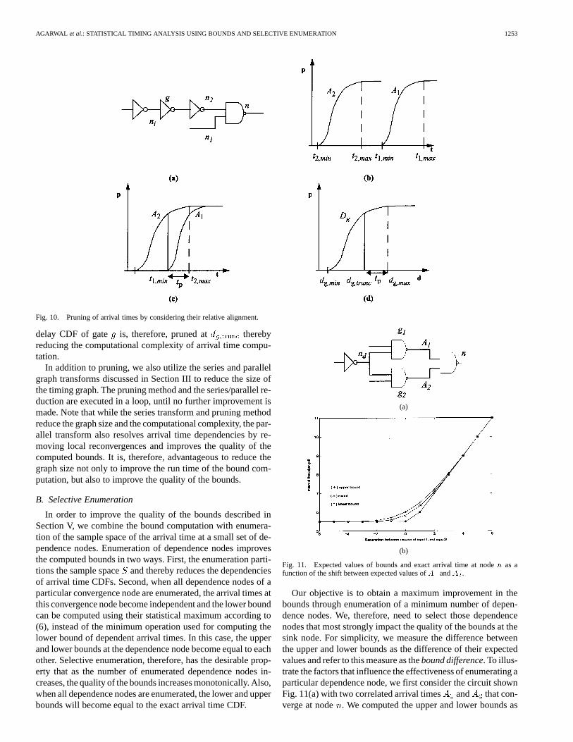
In order to reduce the size of the timing graph, we prune ar-rival times by considering their relative alignment at conver-gence nodes. We consider two arrival time CDFs,andthat converge at node, as shown in Fig. 10(a). If the min-imum arrival time with a nonzero probability of , isgreater than the maximum arrival time with a nonzero proba-bility, of , as shown in Fig. 10(b), it is clear that inthe entire sample space, will be greater than . We can,therefore, prune arrival time from the timing graph withoutchanging its timing behavior. Note that, using this approach, en-tire subgraphs can at times be removed from the timing graph.

Also, when two arrival times and partially overlap, asshown in Fig. 10(c), the CDF of can be truncated at .Based on (6), values of are required only for sincefor , . Hence the CDF of needs to becomputed only for the range to . Based on this, wetruncate the arrival time CDF at fanin nodes of by propa-gating the truncation time across gates in reverse topo-logical order, at each gate subtracting the maximum gate delay

with nonzero probability. The truncation time atnode is, therefore, as follows: , where

is the sum of over all gates between node and .An arrival time at node always results in anarrival at node , such that and can be trun-cated. Furthermore, we also truncate the CDFs of the gate delayfor gates in the fanin cone of . Given a fanin gate withmaximum delay , as shown in Fig. 10(d), the gate delayCDF can be truncated at , where

. Arrival time at is the arrival time whenall fanin gates of have their maximum delay . Hence, itfollows that gate delays less than willalways result in arrival times at that are less than . The


Fig. 10. Pruning of arrival times by considering their relative alignment.

delay CDF of gate is, therefore, pruned at therebyreducing the computational complexity of arrival time compu-tation.

In addition to pruning, we also utilize the series and parallelgraph transforms discussed in Section III to reduce the size ofthe timing graph. The pruning method and the series/parallel re-duction are executed in a loop, until no further improvement ismade. Note that while the series transform and pruning methodreduce the graph size and the computational complexity, the par-allel transform also resolves arrival time dependencies by re-moving local reconvergences and improves the quality of thecomputed bounds. It is, therefore, advantageous to reduce thegraph size not only to improve the run time of the bound com-putation, but also to improve the quality of the bounds.

B. Selective Enumeration

In order to improve the quality of the bounds described inSection V, we combine the bound computation with enumera-tion of the sample space of the arrival time at a small set of de-pendence nodes. Enumeration of dependence nodes improvesthe computed bounds in two ways. First, the enumeration parti-tions the sample spaceand thereby reduces the dependenciesof arrival time CDFs. Second, when all dependence nodes of aparticular convergence node are enumerated, the arrival times atthis convergence node become independent and the lower boundcan be computed using their statistical maximum according to(6), instead of the minimum operation used for computing thelower bound of dependent arrival times. In this case, the upperand lower bounds at the dependence node become equal to eachother. Selective enumeration, therefore, has the desirable prop-erty that as the number of enumerated dependence nodes in-creases, the quality of the bounds increases monotonically. Also,when all dependence nodes are enumerated, the lower and upperbounds will become equal to the exact arrival time CDF.

(a)

(b)

Fig. 11. Expected values of bounds and exact arrival time at noden as afunction of the shift between expected values ofA andA .

Our objective is to obtain a maximum improvement in thebounds through enumeration of a minimum number of depen-dence nodes. We, therefore, need to select those dependencenodes that most strongly impact the quality of the bounds at thesink node. For simplicity, we measure the difference betweenthe upper and lower bounds as the difference of their expectedvalues and refer to this measure as thebound difference. To illus-trate the factors that influence the effectiveness of enumerating aparticular dependence node, we first consider the circuit shownFig. 11(a) with two correlated arrival times and that con-verge at node . We computed the upper and lower bounds as


Fig. 12. Selective enumeration algorithm.

well as the exact arrival time at node, while shifting the align-ment of the CDF of relative to the CDF of , by varyingthe delay of gate . Fig. 11(b) shows the expected value of theupper and lower bounds and the exact arrival time at node,plotted against the difference of the expected value ofand

. As the shift between and increases, the two boundsrapidly converge to the true arrival time. This is caused by thefact that if one arrival time CDF lies significantly after the other,the later arrival time CDF dominates the result and the depen-dence between the two arrival times has little impact. In the ex-treme case, when the minimum time point of the later arrivaltime CDF falls after the maximum time point of the earlier ar-rival time CDF, as shown in Fig. 10(b), the later arrival timepropagates unaltered and the computed bound matches exactlywith the true arrival time distribution.

It is also possible that, two dependent arrival times give rise toa large bound difference at a node, but this bound differencedoes not propagate to the sink node. This occurs when along thepropagation path from to the sink node , the arrival timebounds combine with other arrival time bounds that are alignedsignificantly later and that dominate. In this case, the sink node

is shielded from node and enumeration of its dependencenodes has little impact on the bound difference at. Therefore,enumeration of a dependence node is effective only if its arrivaltime pdfs align at one or more convergence nodes and if the sinknode is not shielded from the arrival times at these convergencenodes.

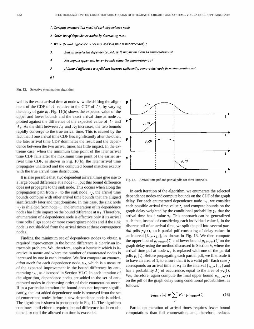
Finding the minimum set of dependence nodes to obtain arequired improvement in the bound difference is clearly an in-tractable problem. We, therefore, apply a heuristic which is it-erative in nature and where the number of enumerated nodes isincreased by one in each iteration. We first compute anenumer-ation merit for each dependence node, which is a measureof the expected improvement in the bound difference by enu-merating , as discussed in Section VI-C. In each iteration ofthe algorithm, dependence nodes are added to the set of enu-merated nodes in decreasing order of their enumeration merit.If in a particular iteration the bound does not improve signifi-cantly, the last added dependence node is removed from the setof enumerated nodes before a new dependence node is added.The algorithm is shown in pseudocode in Fig. 12. The algorithmcontinues until either a required bound difference has been ob-tained, or until the allowed run time is exceeded.

Fig. 13. Arrival time pdf and partial pdfs for three intervals.

In each iteration of the algorithm, we enumerate the selecteddependence nodes and compute bounds on the CDF of the graphdelay. For each enumerated dependence node, we considereach possible arrival time valueand compute bounds on thegraph delay weighted by the conditional probabilitythat thearrival time has a value . This approach can be generalizedsuch that, instead of considering each individual valuein thediscrete pdf of an arrival time, we split the pdf into severalpar-tial pdfs , each partial pdf consisting of delay values inan interval [ ], as shown in Fig. 13. We then computethe upper bound and lower bound on thegraph delay using the method discussed in Section V, where thearrival time pdf at node is replaced with one of the partialpdfs . Before propagating each partial pdf, we first scale itto have an area of 1, to ensure that it is a valid pdf. Each casecorresponds an arrival time at in the interval [ ] andhas a probability of occurrence, equal to the area of .We, therefore, again compute the final upper boundon the pdf of the graph delay using conditional probabilities, asfollows:

(16)

Partial enumeration of arrival times requires fewer boundcomputations than full enumeration, and, therefore, reduces


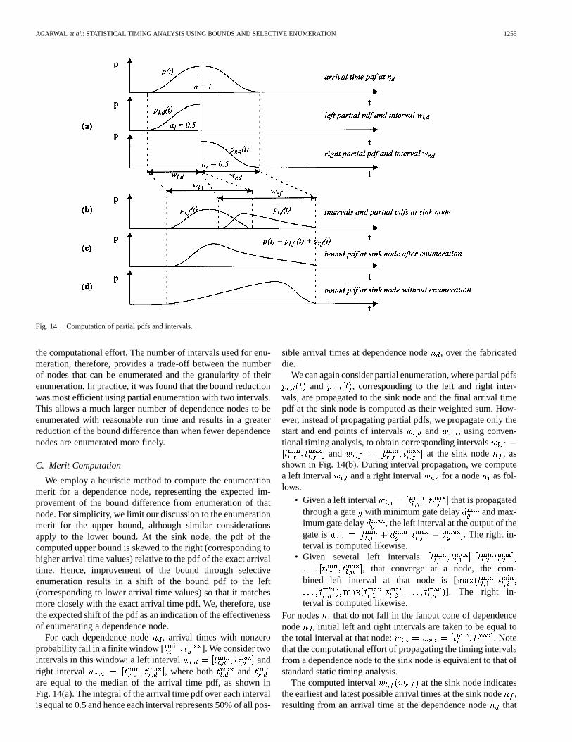
Fig. 14. Computation of partial pdfs and intervals.

the computational effort. The number of intervals used for enu-meration, therefore, provides a trade-off between the numberof nodes that can be enumerated and the granularity of theirenumeration. In practice, it was found that the bound reductionwas most efficient using partial enumeration with two intervals.This allows a much larger number of dependence nodes to beenumerated with reasonable run time and results in a greaterreduction of the bound difference than when fewer dependencenodes are enumerated more finely.

C. Merit Computation

We employ a heuristic method to compute the enumerationmerit for a dependence node, representing the expected im-provement of the bound difference from enumeration of thatnode. For simplicity, we limit our discussion to the enumerationmerit for the upper bound, although similar considerationsapply to the lower bound. At the sink node, the pdf of thecomputed upper bound is skewed to the right (corresponding tohigher arrival time values) relative to the pdf of the exact arrivaltime. Hence, improvement of the bound through selectiveenumeration results in a shift of the bound pdf to the left(corresponding to lower arrival time values) so that it matchesmore closely with the exact arrival time pdf. We, therefore, usethe expected shift of the pdf as an indication of the effectivenessof enumerating a dependence node.

For each dependence node, arrival times with nonzeroprobability fall in a finite window [ ]. We consider twointervals in this window: a left interval andright interval , where both andare equal to the median of the arrival time pdf, as shown inFig. 14(a). The integral of the arrival time pdf over each intervalis equal to 0.5 and hence each interval represents 50% of all pos-

sible arrival times at dependence node, over the fabricateddie.

We can again consider partial enumeration, where partial pdfsand , corresponding to the left and right inter-

vals, are propagated to the sink node and the final arrival timepdf at the sink node is computed as their weighted sum. How-ever, instead of propagating partial pdfs, we propagate only thestart and end points of intervals and , using conven-tional timing analysis, to obtain corresponding intervals

and at the sink node , asshown in Fig. 14(b). During interval propagation, we computea left interval and a right interval for a node as fol-lows.

• Given a left interval that is propagatedthrough a gate with minimum gate delay and max-imum gate delay , the left interval at the output of thegate is . The right in-terval is computed likewise.

• Given several left intervals, that converge at a node, the com-

bined left interval at that node is []. The right in-

terval is computed likewise.For nodes that do not fall in the fanout cone of dependencenode , initial left and right intervals are taken to be equal tothe total interval at that node: . Notethat the computational effort of propagating the timing intervalsfrom a dependence node to the sink node is equivalent to that ofstandard static timing analysis.

The computed interval at the sink node indicatesthe earliest and latest possible arrival times at the sink node,resulting from an arrival time at the dependence nodethat


Fig. 15. Left and right arrival time intervals and bound pdfs.

falls in the interval . Also, the two intervals andat the sink node will overlap, meaning that

due to the uncertainty of gate delays and the merging of inter-vals at convergence nodes. Since the probability of an arrivaltime occurring in either interval or at node is 0.5,the probability of an arrival time occurring in either intervaland at the sink node will be greater than or equal to 0.5, dueto the overlap of the intervals, as shown in Fig. 14(b). Hence,after enumeration of dependence node, the area of the arrivaltime pdf over either interval will be greater or equal to 0.5, asshown in Fig. 14(c). However, due to the inherent error in boundcomputation, the arrival time pdf at the sink node without enu-meration can be significantly skewed to the right, as shown inFig. 14(d). In this case, the area under the left interval can beless than 0.5. Since after enumeration ofthe area under theleft interval will be equal to or greater than 0.5, the amount bywhich the area is less than 0.5 before enumeration is a good indi-cator of the expected shift of the arrival time pdf resulting fromenumeration. The enumeration merit of dependence nodeis,therefore, computed as follows:

ifotherwise

(17)

where is the area of the arrival time pdf at the sink node overthe left interval . Note that the enumerationmerit of a dependence node forlower bound computation canbe computed similarly by observing the amount by which thearrival time pdf at the sink node over the right interval is lessthan 0.5.

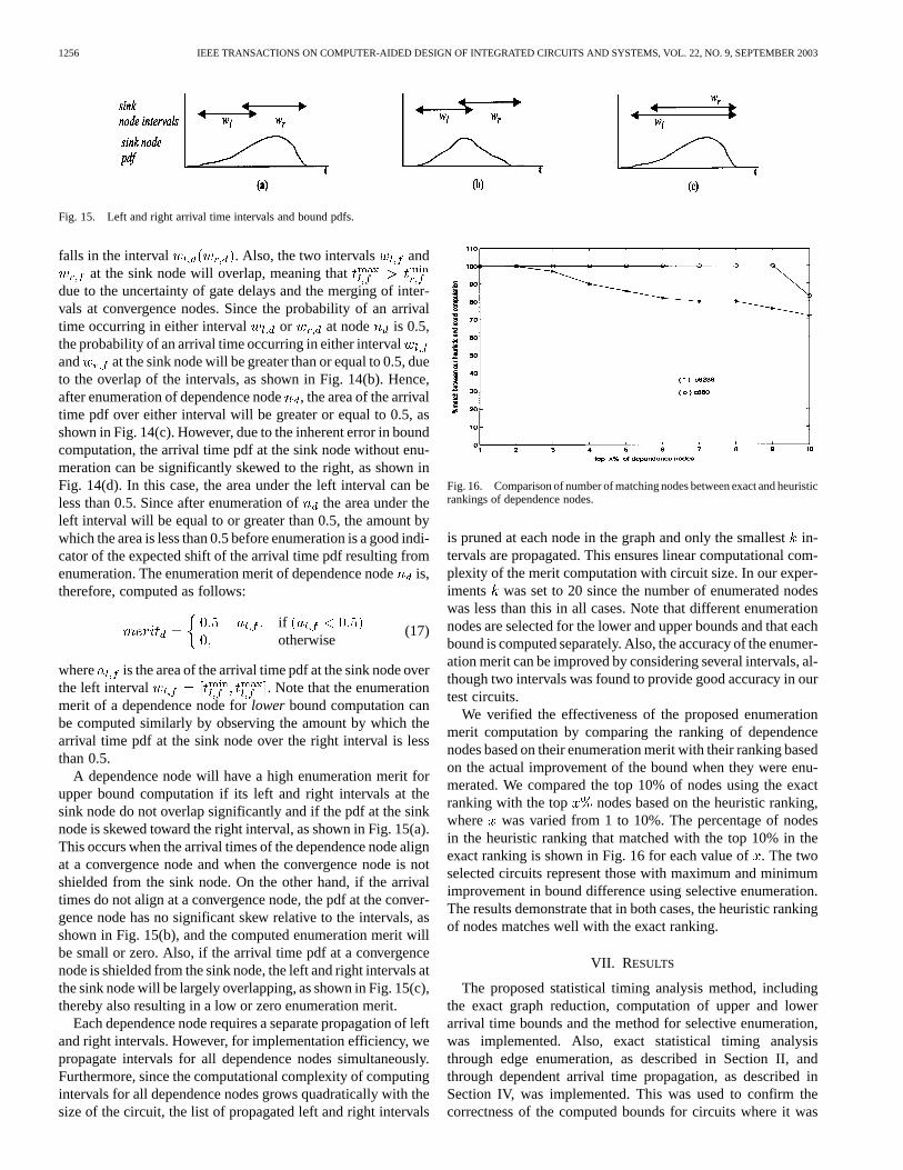
A dependence node will have a high enumeration merit forupper bound computation if its left and right intervals at thesink node do not overlap significantly and if the pdf at the sinknode is skewed toward the right interval, as shown in Fig. 15(a).This occurs when the arrival times of the dependence node alignat a convergence node and when the convergence node is notshielded from the sink node. On the other hand, if the arrivaltimes do not align at a convergence node, the pdf at the conver-gence node has no significant skew relative to the intervals, asshown in Fig. 15(b), and the computed enumeration merit willbe small or zero. Also, if the arrival time pdf at a convergencenode is shielded from the sink node, the left and right intervals atthe sink node will be largely overlapping, as shown in Fig. 15(c),thereby also resulting in a low or zero enumeration merit.

Each dependence node requires a separate propagation of leftand right intervals. However, for implementation efficiency, wepropagate intervals for all dependence nodes simultaneously.Furthermore, since the computational complexity of computingintervals for all dependence nodes grows quadratically with thesize of the circuit, the list of propagated left and right intervals

Fig. 16. Comparison of number of matching nodes between exact and heuristicrankings of dependence nodes.

is pruned at each node in the graph and only the smallestin-tervals are propagated. This ensures linear computational com-plexity of the merit computation with circuit size. In our exper-iments was set to 20 since the number of enumerated nodeswas less than this in all cases. Note that different enumerationnodes are selected for the lower and upper bounds and that eachbound is computed separately. Also, the accuracy of the enumer-ation merit can be improved by considering several intervals, al-though two intervals was found to provide good accuracy in ourtest circuits.

We verified the effectiveness of the proposed enumerationmerit computation by comparing the ranking of dependencenodes based on their enumeration merit with their ranking basedon the actual improvement of the bound when they were enu-merated. We compared the top 10% of nodes using the exactranking with the top nodes based on the heuristic ranking,where was varied from 1 to 10%. The percentage of nodesin the heuristic ranking that matched with the top 10% in theexact ranking is shown in Fig. 16 for each value of. The twoselected circuits represent those with maximum and minimumimprovement in bound difference using selective enumeration.The results demonstrate that in both cases, the heuristic rankingof nodes matches well with the exact ranking.

VII. RESULTS

The proposed statistical timing analysis method, includingthe exact graph reduction, computation of upper and lowerarrival time bounds and the method for selective enumeration,was implemented. Also, exact statistical timing analysisthrough edge enumeration, as described in Section II, andthrough dependent arrival time propagation, as described inSection IV, was implemented. This was used to confirm thecorrectness of the computed bounds for circuits where it was


TABLE ICIRCUIT STATISTICS AND EXACT REDUCTION IMPROVEMENT

TABLE IIRESULTS OFBOUND COMPUTATION AND SELECTIVE ENUMERATION

possible to compute the exact graph delay CDF. For largercircuits, Monte Carlo simulation with 100 000 samples wasused. The statistical timing analysis was tested on the ISCASbenchmark circuits [34]. For each gate in the circuit, a delaydistribution was specified with a standard deviation rangingfrom 10% to 15% of the mean of the distribution. A Gaussiandistribution, truncated at the 3 sigma point, was used. Thisdistribution of gate delay was based on Monte Carlo simulationfor individual gate structures using SPICE simulation. In thesesimulations, intra-die gate length variations were applied, asmeasured for an industrial 0.13m process technology withtest structures on a number of test chips. However, the proposedmethod for statistical timing analysis is not limited to anyparticular type of process variation and can also be used withdelay variations resulting from other process factors.

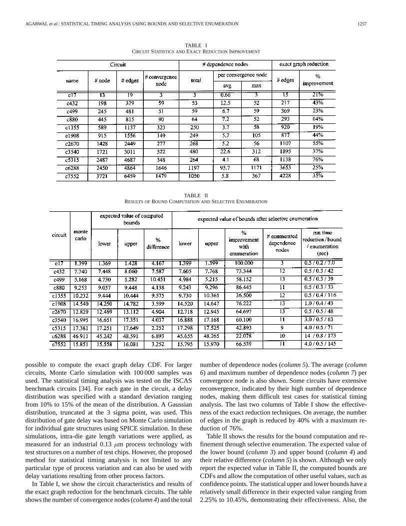
In Table I, we show the circuit characteristics and results ofthe exact graph reduction for the benchmark circuits. The tableshows the number of convergence nodes (column 4) and the total

number of dependence nodes (column 5). The average (column6) and maximum number of dependence nodes (column 7) perconvergence node is also shown. Some circuits have extensivereconvergence, indicated by their high number of dependencenodes, making them difficult test cases for statistical timinganalysis. The last two columns of Table I show the effective-ness of the exact reduction techniques. On average, the numberof edges in the graph is reduced by 40% with a maximum re-duction of 76%.

Table II shows the results for the bound computation and re-finement through selective enumeration. The expected value ofthe lower bound (column 3) and upper bound (column 4) andtheir relative difference (column 5) is shown. Although we onlyreport the expected value in Table II, the computed bounds areCDFs and allow the computation of other useful values, such asconfidence points. The statistical upper and lower bounds have arelatively small difference in their expected value ranging from2.25% to 10.45%, demonstrating their effectiveness. Also, the


Fig. 17. Comparison of CDF bounds and Monte Carlo for c880 and c7552.

Monte Carlo results fall between the computed bounds, as ex-pected.

Table II also shows the bounds after selective enumeration(columns 6 and 7) and the percentage improvement of theirdifference compared to the original bounds (column 8). Thetotal number of dependence nodes enumerated during the boundcomputation is shown in column 9. Excluding the first circuit,where the selective enumeration obtained bounds that exactlymatched the true graph delay, the improvement of the boundsusing selective enumeration ranged between 22.07 – 86.44%,with an average of 62.45%. The number of dependence nodesselected for enumeration was small, ranging from 3 to 13 nodes,showing the somewhat surprising result that enumerating only afew carefully chosen nodes can significantly improve the boundcomputation.

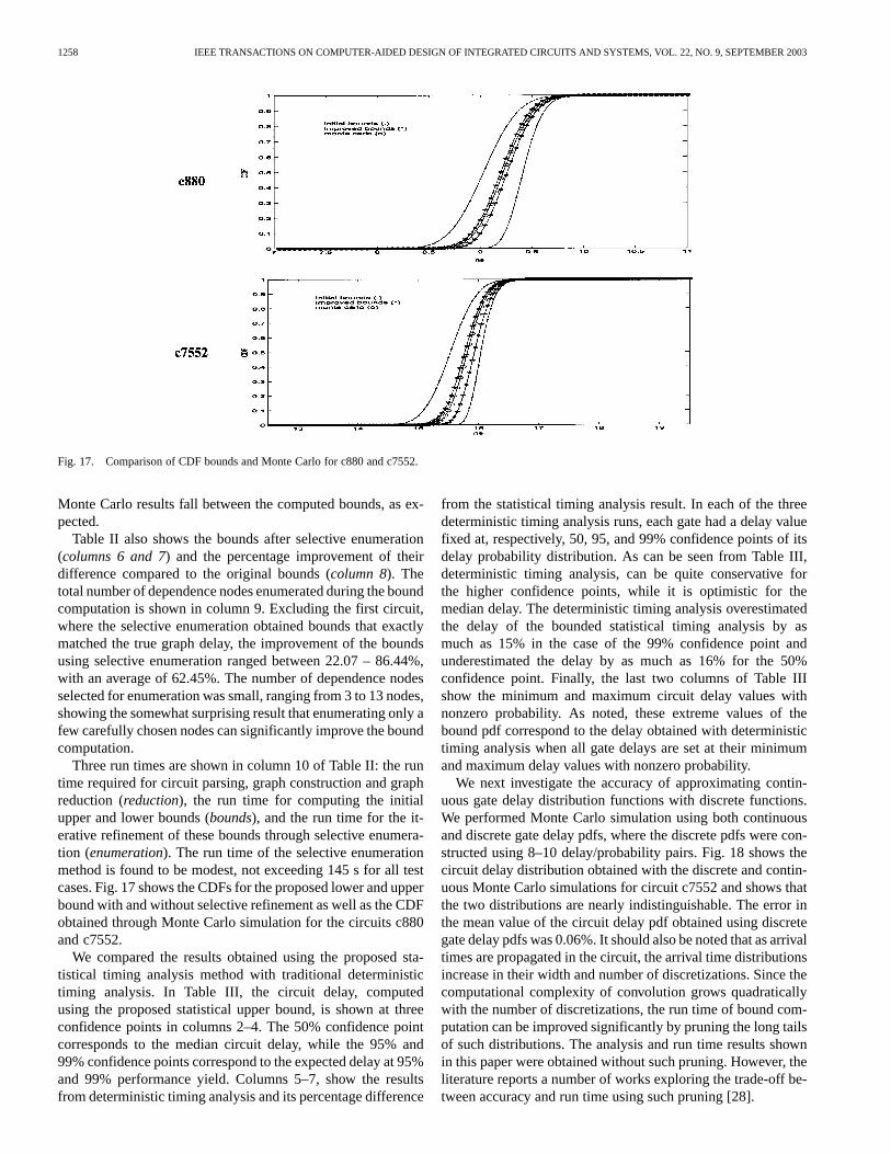
Three run times are shown in column 10 of Table II: the runtime required for circuit parsing, graph construction and graphreduction (reduction), the run time for computing the initialupper and lower bounds (bounds), and the run time for the it-erative refinement of these bounds through selective enumera-tion (enumeration). The run time of the selective enumerationmethod is found to be modest, not exceeding 145 s for all testcases. Fig. 17 shows the CDFs for the proposed lower and upperbound with and without selective refinement as well as the CDFobtained through Monte Carlo simulation for the circuits c880and c7552.

We compared the results obtained using the proposed sta-tistical timing analysis method with traditional deterministictiming analysis. In Table III, the circuit delay, computedusing the proposed statistical upper bound, is shown at threeconfidence points in columns 2–4. The 50% confidence pointcorresponds to the median circuit delay, while the 95% and99% confidence points correspond to the expected delay at 95%and 99% performance yield. Columns 5–7, show the resultsfrom deterministic timing analysis and its percentage difference

from the statistical timing analysis result. In each of the threedeterministic timing analysis runs, each gate had a delay valuefixed at, respectively, 50, 95, and 99% confidence points of itsdelay probability distribution. As can be seen from Table III,deterministic timing analysis, can be quite conservative forthe higher confidence points, while it is optimistic for themedian delay. The deterministic timing analysis overestimatedthe delay of the bounded statistical timing analysis by asmuch as 15% in the case of the 99% confidence point andunderestimated the delay by as much as 16% for the 50%confidence point. Finally, the last two columns of Table IIIshow the minimum and maximum circuit delay values withnonzero probability. As noted, these extreme values of thebound pdf correspond to the delay obtained with deterministictiming analysis when all gate delays are set at their minimumand maximum delay values with nonzero probability.

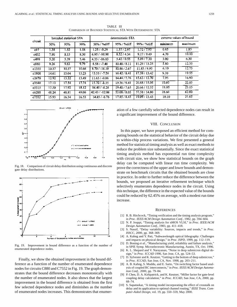
We next investigate the accuracy of approximating contin-uous gate delay distribution functions with discrete functions.We performed Monte Carlo simulation using both continuousand discrete gate delay pdfs, where the discrete pdfs were con-structed using 8–10 delay/probability pairs. Fig. 18 shows thecircuit delay distribution obtained with the discrete and contin-uous Monte Carlo simulations for circuit c7552 and shows thatthe two distributions are nearly indistinguishable. The error inthe mean value of the circuit delay pdf obtained using discretegate delay pdfs was 0.06%. It should also be noted that as arrivaltimes are propagated in the circuit, the arrival time distributionsincrease in their width and number of discretizations. Since thecomputational complexity of convolution grows quadraticallywith the number of discretizations, the run time of bound com-putation can be improved significantly by pruning the long tailsof such distributions. The analysis and run time results shownin this paper were obtained without such pruning. However, theliterature reports a number of works exploring the trade-off be-tween accuracy and run time using such pruning [28].


TABLE IIICOMPARISON OFBOUNDED STATISTICAL STA WITH DETERMINISTIC STA

Fig. 18. Comparison of circuit delay distribution using continuous and discretegate delay distributions.

Fig. 19. Improvement in bound difference as a function of the number ofenumerated dependence nodes.

Finally, we show the obtained improvement in the bound dif-ference as a function of the number of enumerated dependencenodes for circuits C880 and C7552 in Fig. 19. The graph demon-strates that the bound difference decreases monotonically withthe number of enumerated nodes. It also shows that the largestimprovement in the bound difference is obtained from the firstfew selected dependence nodes and diminishes as the numberof enumerated nodes increases. This demonstrates that enumer-

ation of a few carefully selected dependence nodes can result ina significant improvement of the bound difference.

VIII. C ONCLUSION

In this paper, we have proposed an efficient method for com-puting bounds on the statistical behavior of the circuit delay dueto within-chip process variations. We first presented a generalmethod for statistical timing analysis as well as exact methods toreduce the problem size substantially. Since the exact statisticaltiming analysis method has exponential run time complexitywith circuit size, we show how statistical bounds on the graphdelay can be computed with linear run time complexity. Weprove the correctness of the upper and lower bounds and demon-strate on benchmark circuits that the obtained bounds are closein practice. In order to further reduce the difference between thebounds, we proposed an iterative refinement technique whichselectively enumerates dependence nodes in the circuit. Usingthis technique, the difference in the expected value of the boundscould be reduced by 62.45% on average, with a modest run timeincrease.

REFERENCES

[1] R. B. Hitchcock, “Timing verification and the timing analysis program,”in Proc. IEEE/ACM Design Automation Conf., 1982, pp. 594–604.

[2] N. P. Jouppi, “Timing analysis for nMOS VLSI,” inProc. IEEE/ACMDesign Automation Conf., 1983, pp. 411–418.

[3] S. Nassif, “Delay variability: Sources, impacts and trends,” inProc.ISSCC, 2000, pp. 368–369.

[4] A. Kahng and Y. Pati, “Subwavelength optical lithography: Challengesand impacts on physical design,” inProc. ISPD, 1999, pp. 112–119.

[5] D. Boninget al., “Manufacturing yield, reliability and failure analysis,”in SPIE Symp. Microelectronic Manufacturing, Austin, TX, Oct. 1996.

[6] K. L. Shepard and V. Narayanan, “Noise in deep submicron digital de-sign,” in Proc. ICCAD 1996, San Jose, CA, pp. 524–53.

[7] D. Sylvester and K. Keutzer, “Getting to the bottom of deep submicron,”in Proc. ICCAD, San Jose, CA, Nov. 1998, pp. 203–211.

[8] A. B. Kahng, S. Muddu, and E. Sarto, “On switching factor based anal-ysis of coupled RC interconnects,” inProc. IEEE/ACM Design Automa-tion Conf., 2000, pp. 79–84.

[9] P. Chen, D. A. Kirkpatrick, and K. Keutzer, “Miller factor for gate-levelcoupling delay calculation,” inProc. ICCAD, San Jose, CA, 2000, pp.68–74.

[10] S. Sapatnekar, “A timing model incorporating the effect of crosstalk ondelay and its application to optimal channel routing,”IEEE Trans. Com-puter-Aided Design, vol. 19, pp. 550–559, May 2000.


[11] A. Vittal, L. H. Chen, M. Marek-Sadowska, K.-P. Wang, and S. Yang,“Crosstalk in VLSI interconnections,”Trans. Computer-Aided Design,vol. 18, pp. 1817–1824, Dec. 1999.

[12] G. Bai, S. Bobba, and I. N. Hajj, “Static timing analysis includingpower supply noise effect on propagation delay in VLSI circuits,”Proc.IEEE/ACM Design Automation Conf., pp. 295–300, 2001.

[13] K. Bowman, S. Duvall, and J. Meindl, “Impact of die-to-die andwithin-die parameter fluctuations on the maximum clock frequencydistribution,” inProc. ISSCC, San Francisco, CA, 2001, pp. 278–279.

[14] V. Mehrotra, S. Nassif, D. Boning, and J. Chung, “Modeling the effectsof manufacturing variation on high-speed microprocessor interconnectperformance,”IEDM Tech. Dig., pp. 767–770, 1998.

[15] S. R. Nassif, “Modeling and analysis of manufacturing variations,” inProc. CICC, San Diego, CA, 2001, pp. 223–228.

[16] Y. Liu et al., “Model-order reduction of RC(L) interconnect includingvariational analysis,”Proc. IEEE/ACM Design Automation Conf., pp.201–206, 1999.

[17] E. Acaret al., “Assessment of true worst-case circuit performance underinterconnect parameter variations,”Proc. IEEE Int. Symp. Quality Elec-tronic Design, pp. 431–436, 2001.

[18] M. Orshansky, L. Milor, P. Chen, K. Keutzer, and C. Hu, “Impact ofsystematic spatial intra-chip gate length variability on performance ofhigh-speed digital circuits,” inICCAD 2000, San Jose, CA, pp. 62–67.

[19] V. Mehrotra, S. L. Sam, D. Boning, A. Chandrakasan, R. Vallishayee,and S. Nassif, “A methodology for modeling the effects of systematicwithin-die interconnect and device variation on circuit performance,” inProc. IEEE/ACM Design Automation Conf., Los Angeles, CA, 2000, pp.172–175.

[20] Y. Deguchi, N. Ishiura, and S. Yajima, “Probabilistic CTSS: Analysisof timing error probability in asynchronous logic circuits,”Proc.IEEE/ACM Design Automation Conf., pp. 650–655, 1991.

[21] S. Devadas, H. F. Jyu, K. Keutzer, and S. Malik, “Statistical timing anal-ysis of combinational circuits,” inProc. ICCD 1992, Cambridge, MA,pp. 38–43.

[22] H. F. Jyu and S. Malik, “Statistical timing optimization of combinationallogic circuits,” inProc. ICCD 1993, Cambridge, MA, pp. 77–80.

[23] R. B. Brawhear, N. Menezes, C. Oh, L. Pillage, and R. Mercer, “Pre-dicting circuit performance using circuit-level statistical timing anal-ysis,” in Proc. Eur. Design and Test Conf., Paris, France, 1994.

[24] M. Berkelaar, “Statistical delay calculation, A linear time method,” inProc. TAU 97, Austin, TX, Dec. 1997, pp. 15–24.

[25] E. T. A. F. Jacobs and M. R. C. M. Berkelaar, “Gate sizing using a statis-tical delay model,”Proc. IEEE/ACM Design Automation and Test Eur.Conf., pp. 283–290, 2000.

[26] R.-B. Lin and M.-C. Wu, “A new statistical approach to timing analysisof VLSI circuits,” in Proc. Int. Conf. VLSI Design, Chennai, India, 1998,pp. 507–513.

[27] S. Tongsima, C. Chantrapornchai, E. H.-M. Sha, and N. L. Passos,“Optimizing circuits with confidence probability using probabilisticretiming,” Proc. IEEE ISCAS, pp. 270–273, 1998.

[28] J. J. Liou, K. T. Cheng, S. Kundu, and A. Krstic, “Fast statistical timinganalysis by probabilistic even propagation,” inProc. IEEE/ACM DesignAutomation Conf., Las Vegas, NV, 2001, pp. 661–666.

[29] J.-J. Liou, A. Krstic, L.-C. Wang, and K.-T. Cheng, “False path awarestatistical timing analysis and efficient path selection for delay testingand timing validation,”Proc. ACM/IEEE Design Automation Conf., pp.566–569, 2002.

[30] M. Orshansky and K. Keutzer, “A general probabilistic framework forworst-case timing analysis,” inProc. ACM/IEEE Design AutomationConf., New Orleans, LA, 2002, pp. 556–569.

[31] A. Gattiker, S. Nassif, R. Dinakar, and C. Long, “Timing yield estima-tion from static timing analysis,” inProc. ISQED 2001, San Jose, CA,pp. 437–442.

[32] X. Bai, C. Visweswariah, P. Strenski, and D. Hathaway, “Uncertainty-aware circuit optimization,”Proc. ACM/IEEE Design Automation Conf.,pp. 58–63, 2002.

[33] F. Najm, R. Burch, P. Yang, and I. Hajj, “Probabilistic simulation for re-liability analysis of CMOS VLSI circuits,”IEEE Trans.Computer-AidedDesign, vol. 9, Apr. 1990.

[34] F. Brglez and H. Fujiwara, “A neutral netlist of 10 combinatorial bench-mark circuits,”Proc. IEEE ISCAS, pp. 695–698, 1985.

[35] W. P. Feller,An Introduction to Probability Theory and its Applica-tions. New York: Wiley, 1970, vol. 1–2.

Aseem Agarwal (S’03) received the B.E. degreein electronics and communication from GujaratUniversity, India, in 2001. Since August 2001, heis a Doctoral Student in Department of ElectricalEngineering and Computer Science at University ofMichigan, Ann Arbor.

He is a Research Assistant in the AdvancedComputer Architecture Lab working with Prof. D.Blaauw. His research focuses on timing analysismodels and algorithms that consider processvariability.

Vladimir Zolotov (M’97) received the Engineerdegree from the Moscow Institute of Electronics,Moscow, Russia, and the Ph.D. degree from theScientific Research Institute of Micro Devices,Moscow, Russia, both in electrical engineering.

He has been with the Advanced Tools Group,Motorola, Inc., Austin, TX, since 1998. He isinvolved in the development of EDA tools andmethodology for high-performance VLSI designs.Previously, he was with the Moscow ResearchLaboratory, Motorola, Inc., Moscow, Russia. His

research interests include signal integrity, reliability, on-chip inductance,timing analysis, and optimization of VLSI.

David T. Blaauw (M’01) received the B.S. degreein physics and computer science from Duke Univer-sity, Durham, NC, in 1986, and the M.S. and Ph.D.degrees in computer science from the University ofIllinois, Urbana, in 1988 and 1991, respectively.

He was with the Engineering Accelerator Tech-nology Division, IBM Corporation, Endicott, NY,as a Development Staff Member, until August 1993.From 1993 to August 2001, he was with Motorola,Inc., Austin, TX, where he was the Manager ofthe High Performance Design Technology Group.

Since August 2001, he has been a member of the faculty at the Universityof Michigan, Ann Arbor, as an Associate Professor. His work has focusedon VLSI design and CAD with particular emphasis on circuit analysis andoptimization problems for high-performance and low-power designs.

Dr. Blaauw was the Technical Program Chair and General Chair for the Inter-national Symposium on Low Power Electronics and Design, in 1999 and 2000,respectively, and was the Technical Program Co-Chair and member of the Ex-ecutive Committee of the ACM/IEEE Design Automation Conference in 2000and 2001.

Documents

Statistical timing analysis using bounds and selective …blaauw.engin.umich.edu/wp-content/uploads/sites/342/2017/11/39.pdf · static timing analysis (STA) using so-called case analysis