Statistical properties of turbulence: An overview · 2019-04-09 · Statistical properties of turbulence: An overview RAHUL PANDIT1,∗, PRASAD PERLEKAR and SAMRIDDHI SANKAR RAY Centre

Statistical properties of turbulence:An overview

RAHUL PANDIT1,∗, PRASAD PERLEKAR and SAMRIDDHI SANKAR RAY

Centre for Condensed Matter Theory, Department of Physics, Indian Institute of Science,Bangalore 560 012, India

1Also at: Jawaharlal Nehru Centre for Advanced Scientific Research, Jakkur, Bangalore 560 064, India∗e-mail: [email protected]

We present an introductory overview of several challenging problems in the statistical characteri-zation of turbulence. We provide examples from fluid turbulence in three and two dimensions, fromthe turbulent advection of passive scalars, turbulence in the one-dimensional Burgers equation, andfluid turbulence in the presence of polymer additives.

1. Introduction

Turbulence is often described as the last greatunsolved problem of classical physics [1–3].However, it is not easy to state what would consti-tute a solution of the turbulence problem. This isprincipally because turbulence is not one problembut a collection of several important problems:These include the characterization and control ofturbulent flows, both subsonic and supersonic, ofinterest to engineers such as flows in pipes orover cars and aeroplanes [4,5]. Mathematical ques-tions in this area are concerned with develop-ing proofs of the smoothness, or lack thereof, ofsolutions of the Navier–Stokes and related equa-tions [6–10]. Turbulence also provides a variety ofchallenges for fluid dynamicists [5,11–13], astro-physicists [14–17], geophysicists [18,19], climatescientists [20], plasma physicists [15–17,21,22],and statistical physicists [23–32]. In this briefoverview, written primarily for physicists whoare not experts in turbulence, we concentrate onsome recent advances in the statistical characteri-zation of fluid turbulence [33] in three dimen-sions, the turbulence of passive scalars such aspollutants [34], two-dimensional turbulence in thinfilms or soap films [35,36], turbulence in theBurgers equation [37–39], and fluid turbulence

with polymer additives [40–42]; in most ofthis paper we restrict ourselves to homoge-neous, isotropic turbulence [33,43,44]; and wehighlight some similarities between the stati-stical properties of systems at a critical pointand those of turbulent fluids [31,45,46]. Severalimportant problems that we do not attempt tocover include Rayleigh–Benard turbulence [47],superfluid turbulence [3,48], magnetohydrodyan-mic turbulence [15,17,21,22], the behaviour ofinertial particles in turbulent flows [49], the tran-sition to turbulence in different experimentalsituations [50,51], and boundary-layer [52,53] andwall-bounded [54] turbulence.

This paper is organized as follows: Section 2 givesan overview of some of the experiments of rele-vance to our discussion here. In §3 we introduce theequations that we consider. Section 4 is devoted toa summary of phenomenological approaches thathave been developed, since the pioneering studiesof Richardson [55] and Kolmogorov [56], in 1941(K41), to understand the behaviour of velocityand other structure functions in inertial ranges.Section 5 introduces the ideas of multiscaling thathave been developed to understand deviationsfrom the predictions of K41-type phenomenology.Section 6 contains illustrative direct numericalsimulations; it consists of five subsections devoted

Keywords. Statistical properties of turbulence.

339

340 RAHUL PANDIT et al

to (a) three-dimensional fluid turbulence, (b) shellmodels, (c) two-dimensional turbulence in soapfilms, (d) turbulence in the one-dimensionalBurgers equation, and (e) fluid turbulence withpolymer additives. Section 7 contains concludingremarks.

2. Experimental overview

Turbulent flows abound in nature. They includethe flow of water in a garden pipe or in rapids,the flow of air over moving cars or aeroplanes, jetsthat are formed when a fluid is forced through anorifice, the turbulent advection of pollutants suchas ash from a volcanic eruption, terrestrial andJovian storms, turbulent convection in the Sun,and turbulent shear flows in the arms of spiralgalaxies. A wide variety of experimental studieshave been carried out to understand the propertiesof such turbulent flows; we concentrate on thosethat are designed to elucidate the statistical pro-perties of turbulence, especially turbulence that is,at small spatial scales and far away from bound-aries, homogeneous and isotropic. Most of our dis-cussion will be devoted to incompressible flows, i.e.,low-Mach-number cases in which the fluid velo-city is much less than the velocity of sound in thefluid.

In laboratories such turbulence is generated inmany different ways. A common method uses a gridin a wind tunnel [57]; the flow downstream fromthis grid is homogeneous and isotropic, to a goodapproximation. Another technique use the vonKarman swirling flow, i.e., flow generated in a fluidcontained in a cylindrical tank with two coaxial,counter-rotating discs at its ends [58–60]; in themiddle of the tank, far away from the discs, theturbulent flow is approximately homogeneous andisotropic. Electromagnetically forced thin films andsoap films [1,35,36] have yielded very useful resultsfor two-dimensional turbulence. Turbulence datacan also be obtained from atmospheric boundarylayers [61–64], oceanic flows [65], and astrophysicalmeasurements [14]; experimental conditions cannotbe controlled as carefully in such natural settingsas they can be in a laboratory, but a far greaterrange of length scales can be probed than is possi-ble in laboratory experiments.

Traditionally, experiments have measured thevelocity u(x, t) at a single point x at various timest by using hot-wire anemometers; these anemome-ters can have limitations in (a) the number of com-ponents of the velocity that can be measured and(b) the spatial and temporal resolutions that canbe obtained [66,67]. Such measurements yield atime series for the velocity; if the mean flow velo-city U � urms, the root-mean-square fluctuations

of the velocity, then Taylor’s frozen-flow hypothe-sis [5,33] can be used to relate temporal separa-tions δt to spatial separations δr, along the meanflow direction via δr = Uδt. The Reynolds num-ber Re = UL/ν, where U and L are typical velo-city and length scales in the flow and ν is thekinematic viscosity, is a convenient dimensionlesscontrol parameter; at low Re flows are laminar;as it increases, there is a transition to turbulenceoften via a variety of instabilities [50] that wewill not cover here; and at large Re fully deve-loped turbulence sets in. To compare different flowsit is often useful to employ the Taylor-microscaleReynolds number Reλ = urmsλ/ν, where the Taylormicroscale λ can be obtained from the energy spec-trum described below in §6.3.

Refinements in hot-wire anemometry [63,68] andflow visualization techniques such as laser-Dopplervelocimetry (LDV) [66], particle-image velocime-try (PIV) [66,67], particle-tracking velocimetry(PTV) [66,67], tomographic PIV [69], holographicPIV [70], and digital holographic microscopy [71]have made it possible to obtain reliable measure-ments of the Eulerian velocity u(x, t) (see §3) in aturbulent flow. In the simplest forms of anemome-try, a time series of the velocity is obtained at agiven point in space; in PIV two components ofthe velocity field can be obtained in a sheet at agiven time; holographic PIV can yield all compo-nents of the velocity field in a volume. Componentsof the velocity derivative tensor Aij ≡ ∂jui canalso be obtained [63] and hence quantities suchas the energy dissipation rate per unit mass perunit volume ε ≡ ν〈

∑i,j(∂iuj + ∂jui)2〉, the vorti-

city ω = ∇× u, and components of the rate ofstrain tensor sij ≡ (∂iuj + ∂jui)/2, where the sub-scripts i and j are Cartesian indices. A discussion ofthe subtleties and limitations of these measurementtechniques lies beyond the scope of our overview;we refer the reader to refs [63,66,67] for details.Significant progress has also been made over thepast decade in the measurement of Lagrangian tra-jectories (see §3) of tracer particles in turbulentflows [58,59]. Given such measurements, experi-mentalists can obtain several properties of turbu-lent flows. We give illustrative examples of thetypes of properties we consider.

Flow visualization methods often displaylarge-scale coherent structures in turbulentflows. Examples of such structures are plumesin Rayleigh–Benard convection [72], structuresbehind a splitter plate [73], and large vorti-cal structures in two-dimensional or stratifiedflows [1,35,36]. In three-dimensional flows, as wewill see in greater detail below, energy that ispumped into the flow at the injection scale Lcascades, as first suggested by Richardson [55],from large-scale eddies to small-scale ones till it

STATISTICAL PROPERTIES OF TURBULENCE: AN OVERVIEW 341

is eventually dissipated around and beyond thedissipation scale ηd. By contrast, two-dimensionalturbulence [35,36,74,75] displays a dual cascade:there is an inverse cascade of energy from the scaleat which it is pumped into the system to largelength scales and a direct cascade of enstrophyΩ = 〈1

2ω2〉 to small length scales. The inverse cas-

cade of energy is associated with the formationof a few large vortices; in practical realizationsthe sizes of such vortices are controlled finally byEkman friction that is induced, e.g., by air drag insoap-film turbulence.

Measurements of the vorticity ω in highly tur-bulent flows show that regions of large ω are orga-nized into slender tubes. The first experimentalevidence for this was obtained by seeding the flowwith bubbles that moved preferentially to regionsof low pressure [76] that are associated with large-ω regimes. For recent experiments on vortex tubeswe refer the reader to ref. [77].

The time series of the fluid velocity at a givenpoint x shows strong fluctuations. It is natural,therefore, to inquire into the statistical proper-ties of turbulent flows. From the Eulerian velocityu(x, t) and its derivatives we can obtain one-pointstatistics, such as probability distribution functions(PDFs) of the velocity and its derivatives. VelocityPDFs are found to be close to Gaussian distribu-tions. However, PDFs of ω2 and velocity derivativesshow significant non-Gaussian tails; for a recentstudy, which contains references to earlier work, seeref. [63]. The PDF of ε is non-Gaussian too and thetime series of ε is highly intermittent [78]; further-more, in the limit Re → ∞, i.e., ν → 0, the energydissipation rate per unit volume ε approaches apositive constant value (see figure 2 of ref. [79]),a result referred to as a dissipative anomaly or thezeroth law of turbulence.

Various statistical properties of the rate-of-straintensor, with components sij, have been mea-sured [63]. The eigenvalues λ1, λ2, and λ3, withλ1 > λ2 > λ3, of this tensor must satisfy λ1 + λ2+λ3 = 0, with λ1 > 0 and λ2 < 0, in an incompress-ible flow. The sign of λ2 cannot be determined bythis condition but its PDF shows that, in turbu-lent flows, λ2 has a small, positive mean value [80];and the PDFs of cos(ω · ei), where ei is the nor-malized eigenvector corresponding to λi, show thatthere is a preferential alignment [63] of ω and e2.Joint PDFs can be measured too with good accu-racy. An example of recent interest is a tear-dropfeature observed in contour plots of the joint PDFof, respectively, the second and third invariants,Q = −tr(A2)/2 and R = −tr(A3)/3 of the velo-city gradient tensor Aij (see figure 11 of ref. [63]);we display such a plot in §6 that deals with directnumerical simulations.

Two-point statistics are characterized conven-tionally by studying the equal-time, order-p, longi-tudinal velocity structure function

Sp(r) = 〈[(u(x + r) − u(x)) · (r/r)]p〉, (1)

where the angular brackets indicate a time aver-age over the nonequilibrium statistical steady statethat we obtain in forced turbulence (decaying tur-bulence is discussed in §6.2). Experiments [33,81]show that, for separations r in the inertial rangeηd r L,

Sp(r) ∼ rζp , (2)

with exponents ζp that deviate significantly fromthe simple scaling prediction [56] ζK41

p = p/3, espe-cially for p > 3, where ζp < ζK41

p . This prediction,made by Kolmogorov in 1941 (hence the abbrevi-ation K41), is discussed in §4; the deviations fromthis simple scaling prediction are referred to asmultiscaling (§5) and they are associated with theintermittency of ε mentioned above. We mention,in passing, that the log-Poisson model due to Sheand Leveque provides a good parametrization ofthe plot of ζp vs. p [82].

The second-order structure function S2(r) canbe related easily by Fourier transformation to theenergy spectrum E(k) = 4πk2〈|u(k)|2〉, where thetilde denotes the Fourier transform, k = |k|, k isthe wave vector, we assume that the turbulenceis homogeneous and isotropic, and, for specificity,we give the formula for the three-dimensional case.Since ζK41

2 = 2/3, the K41 prediction is

EK41(k) ∼ k−5/3, (3)

a result that is in good agreement with a wide rangeof experiments (see refs [33,83]).

The structure functions Sp(r) are the momentsof the PDFs of the longitudinal velocity incrementsδu|| ≡ [(u(x + r) − u(x)) · (r/r)]. (In the argumentof Sp we use r instead of r when we consider homo-geneous, isotropic turbulence.) These PDFs havebeen measured directly [84] and they show non-Gaussian tails; as r decreases, the deviations ofthese PDFs from Gaussian distributions increases.

We now present a few examples of recentLagrangian measurements [58,59] that have beendesigned to track tracer particles in, e.g., thevon Karman flow at large Reynolds numbers.By employing state-of-the-art measurement tech-niques, such as silicon strip detectors [59], usedin high-energy-physics experiments, or acoustic-Doppler methods [58], these experiments have beenable to attain high spatial resolution and highsampling rates and have, therefore, been able toobtain good data for acceleration statistics ofLagrangian particles and the analogues of velocitystructure functions for them.


These experiments [59] find, for 500 < Reλ <970, consistency with the Heisenberg–Yaglom scal-ing form of the acceleration variance, i.e.,

〈aiaj〉 ∼ ε(3/2)ν(−1/2)δij , (4)

where ai is the Cartesian component i of theacceleration. Furthermore, there are indications ofstrong intermittency effects in the acceleration ofparticles and anisotropy effects are present even atvery large Reλ.

Order-p Lagrangian velocity structure functionsare defined along a Lagrangian trajectory as

SLi,p(τ) = 〈[vL

i (t+ τ) − vLi (t)]p〉, (5)

where the superscript L denotes Lagrangianand the subscript i the Cartesian component.If the time lag τ lies in the temporal analogueof the inertial range, i.e., τη τ TL, where τη

is the viscous dissipation time scale and TL is thetime associated with the scale L at which energy isinjected into the system, then it is expected that

SLi,p(τ) ∼ τ ζL

i,p . (6)

The analogue of the dimensional K41 predictionis ζL,K41

i,p = p/2; experiments and simulations [60]indicate that there are corrections to this simpledimensional prediction.

The best laboratory realizations of two-dimensional turbulence are (a) a thin layer of aconducting fluid excited by magnetic fields, vary-ing both in space and time and applied perpen-dicular to the layer [85] and (b) soap films [86] inwhich turbulence can be generated either by elec-tromagnetic forcing or by the introduction of acomb, which plays the role of a grid, in a rapidlyflowing soap film. In the range of parameters usedin typical experimental studies [1,35,36,87] boththese systems can be described quite well [88,89]by the 2D Navier–Stokes equation (see §3) withan additional Ekman friction term, induced typi-cally by air drag; however, in some cases we mustalso account for corrections arising from fluctua-tions of the film thickness, compressibility effects,and the Marangoni effect. Measurement techniquesare similar to those employed to study three-dimensional turbulence [1,35,36]. Two-dimensionalanalogues of the PDFs described above for 3D tur-bulence have been measured (see ref. [87]); we willtouch on these briefly when we discuss numericalsimulations of 2D turbulence in §6.3. Velocity andvorticity structure functions can be measured as in3D turbulence. However, inertial ranges associatedwith inverse and forward cascades must be distin-guished; the former shows simple scaling with anenergy spectrum E(k) ∼ k−5/3 whereas the latterhas an energy spectrum E(k) ∼ k−(3+δ), with δ = 0

if there is no Ekman friction and δ > 0 otherwise.In the forward cascade velocity structure func-tions show simple scaling [87]; we are not aware ofexperimental measurements of vorticity structurefunctions (we will discuss these in the context ofnumerical simulations in §6.3).

We end this section with a brief discussion ofone example of turbulence in a non-Newtoniansetting, namely, fluid flow in the presence of poly-mer additives. There are two dimensionless controlparameters in this case: Re and the Weissenbergnumber We, which is a ratio of the polymer relaxa-tion time and a typical shearing time in theflow (some studies [41] use a similar dimension-less parameter called the Deborah number De).Dramatically different behaviours arise dependingon the values of these parameters.

In the absence of polymers the flow is laminarat low Re; however, the addition of small amountsof high-molecular-weight polymers can induce elas-tic turbulence [90], i.e., a mixing flow that is liketurbulence and in which the drag increases withincreasing We. We will not discuss elastic turbu-lence in detail here; we refer the reader to ref. [90]for an overview of experiments and to ref. [91] forrepresentative numerical simulations.

If, instead, the flow is turbulent in the absence ofpolymers, i.e., we consider large-Re flows, then theaddition of polymers leads to the dramatic pheno-menon of drag reduction that has been known since1949 [92]; it has obvious and important industrialapplications [40,41,93–95]. Normally drag reduc-tion is discussed in the context of pipe or channelflows: on the addition of polymers to turbulent flowin a pipe, the pressure difference required to main-tain a given volumetric flow rate decreases, i.e., thedrag is reduced and a percentage drag reductioncan be obtained from the percentage reduction inthe pressure difference. For a recent discussion ofdrag reduction in pipe or channel flows we refer thereader to ref. [41]. Here we concentrate on otherphenomena that are associated with the additionof polymers to turbulent flows that are homogene-ous and isotropic. In particular, experiments [93]show that the polymers lead to a suppression ofsmall-scale structures and important modificationsin the second-order structure function [96]. Wewill return to an examination of such phenom-ena when we discuss direct numerical simulationsin §6.5.

3. Models

Before we discuss advances in the statisticalcharacterization of turbulence, we provide a briefdescription to the models we consider. We startwith the basic equations of hydrodynamics, in


three and two dimensions, that are central tothe studies of turbulence. We also give introduc-tory overviews of the Burgers equation in onedimension, the advection–diffusion equation forpassive scalars, and the coupled NS and finitelyextensible nonlinear elastic Peterlin (FENE-P)equations for polymers in a fluid. We end this sec-tion with a description of shell models that areoften used as highly simplified models for homoge-neous, isotropic turbulence.

At low Mach numbers, fluid flows are governedby the Navier–Stokes (NS) eq. (7) augmented bythe incompressibility condition

∂tu + (u · ∇)u = −∇p+ ν∇2u + f ,

∇ · u = 0, (7)

where we use units in which the density ρ = 1,the Eulerian velocity at point r and time t isu(r, t), the external body force per unit volume isf , and ν is the kinematic viscosity. The pressurep can be eliminated by using the incompressibilitycondition [5,33,43] and it can then be obtainedfrom the Poisson equation ∇2p = −∂ij(uiuj). Inthe unforced, inviscid case, the momentum, thekinetic energy, and the helicity H ≡

∫drω · u/2

are conserved; here ω ≡ ∇× u is the vorticity. TheReynolds number Re ≡ LV/ν, where L and V arecharacteristic length and velocity scales, is a con-venient dimensionless control parameter: The flowis laminar at low Re and irregular, and eventuallyturbulent, as Re is increased.

In the vorticity formulation the NS equation (7)becomes

∂tω = ∇× u × ω + ν∇2ω + ∇× f ; (8)

the pressure is eliminated naturally here. This for-mulation is particularly useful is two dimensionssince ω is pseudo-scalar in this case. Specifically, intwo dimensions, the NS equation can be written interms of ω and the stream function ψ:

∂tω − J(ψ,ω) = ν∇2ω + αEω + f ;

∇2ψ = ω;

J(ψ,ω) ≡ (∂xψ)(∂yω) − (∂xω)(∂yψ). (9)

Here αE is the coefficient of the air-drag-inducedEkman friction term. The incompressibility con-straint

∂xux + ∂yuy = 0 (10)

ensures that the velocity is uniquely determined byψ via

u ≡ (−∂yψ, ∂xψ). (11)

In the inviscid, unforced case we have more con-served quantities in two dimensions than in three;

the additional conserved quantities are 〈12ωn〉, for

all powers n, the first of which is the mean enstro-phy, Ω = 〈1

2ω2〉.

In one dimension (1D) the incompressibility con-straint leads to trivial velocity fields. It is fruit-ful, however, to consider the Burgers equation [37],which is the NS equation without pressure andthe incompressibility constraint. This has beenstudied in great detail as it often provides interest-ing insights into fluid turbulence. In 1D the Burgersequation is

∂tv + v∂xv = ν∇2v + f, (12)

where f is the external force and the velocityv can have shocks since the system is compress-ible. In the unforced, inviscid case the Burgersequation has infinitely many conserved quantities,namely,

∫vndx for all integers n. In the limit

ν → 0 we can use the Cole–Hopf transformation,v = ∂xΨ, f ≡ −∂xF , and Ψ ≡ 2ν ln Θ, to obtain∂tΘ = ν∂2

xΘ + FΘ/(2ν), a linear partial differen-tial equation (PDE) that can be solved explicitlyin the absence of any boundary [38,39].

Passive scalars such as pollutants can beadvected by fluids. These flows are governed by theadvection–diffusion equation

∂tθ + u · ∇θ = κ∇2θ + fθ, (13)

where θ is the passive scalar field, the advectingvelocity field u satisfies the NS equation (7), and fθis an external force. The field θ is passive because itdoes not act on or modify u. Note that eq. (13) islinear in θ. It is possible, therefore, to make consi-derable analytical progress in understanding thestatistical properties of passive scalar turbulencefor the simplified model of passive scalar advec-tion due to Kraichnan [34,97]. In this model eachcomponent of fθ is a zero mean Gaussian randomvariable that is white in time. Furthermore, eachcomponent of u taken to be a zero mean Gaussianrandom variable that is white in time has thecovariance

〈ui(x, t)uj(x + r, t′)〉 = 2Dijδ(t− t′). (14)

The Fourier transform of Dij has the form

Dij(q) ∝(

q2 +1L2

)−(d+ξ)/2

e−ηq2

[

δij −qiqj

q2

]

;

(15)

q is the wave vector, L is the characteristic largelength scale, η is the dissipation scale, and ξ is aparameter. In the limit of L→ ∞ and η → 0 wehave, in real space,

Dij(r) = D0δij −12dij(r) (16)


with

dij = D1rξ[(d− 1 + ξ)δij − ξ

rirj

r2

]. (17)

D1 is a normalization constant and ξ a parame-ter; for 0 < ξ < 2 equal-time passive-scalar struc-ture functions show multiscaling [34].

We turn now to an example of a model fornon-Newtonian flows. This model combines the NSequation for a fluid with the finitely extensible non-linear elastic Peterlin (FENE-P) model for poly-mers; it is used inter alia to study the effects ofpolymer additives on fluid turbulence. This modelis defined by the following equations:

∂tu + (u · ∇)u = ν∇2u +μ

τP∇ · [f(rP)C] −∇p,

(18)

∂tC + u · ∇C = C · (∇u) + (∇u)T · C − f(rP)C − IτP

.

(19)

Here ν is the kinematic viscosity of the fluid, μ theviscosity parameter for the solute (FENE-P), τPthe polymer relaxation time, ρ the solvent density,p the pressure, (∇u)T the transpose of (∇u), Cαβ ≡〈RαRβ〉 the elements of the polymer-conformationtensor C (angular brackets indicate an averageover polymer configurations), I the identity tensorwith elements δαβ, f(rP) ≡ (L2 − 3)/(L2 − r2

P) theFENE-P potential that ensures finite extensibility,rP ≡

√Tr(C) and L the length and the maximum

possible extension, respectively, of the polymers,and c ≡ μ/(ν + μ) a dimensionless measure of thepolymer concentration [98].

The hydrodynamical partial differential equa-tions (PDEs) discussed above are difficult to solve,even on computers via direct numerical simulation(DNS), if we want to resolve the large ranges ofspatial and temporal scales that become relevant inturbulent flows. It is useful, therefore, to considersimplified models of turbulence that are numeri-cally more tractable than these PDEs. Shell modelsare important examples of such simplified mod-els; they have proved to be useful testing groundsfor the multiscaling properties of structure func-tions in turbulence. We will consider, as illustrativeexamples, the Gledzer–Ohkitani–Yamada (GOY)shell model [99] for fluid turbulence in three dimen-sions and a shell model for the advection–diffusionequation [100].

Shell models cannot be derived from the NSequation in any systematic way. They are formu-lated in a discretized Fourier space with logarith-mically spaced wave vectors kn = k0λ

n, λ > 1, asso-ciated with shells n and dynamical variables that

are the complex, scalar velocities un. Note thatkn is chosen to be a scalar: spherical symmetry isimplicit in GOY-type shell models since their aim isto study homogeneous, isotropic turbulence. Giventhat kn and un are scalars, shell models cannotdescribe vortical structures or enforce the incom-pressibility constraint.

The temporal evolution of such a shell modelis governed by a set of ordinary differential equa-tions that have the following features in commonwith the Fourier-space version of the NS equa-tion [12]: they have a viscous dissipation termof the form −νk2

nun, they conserve the shell-model analogues of the energy and the helicityin the absence of viscosity and forcing, and theyhave nonlinear terms of the form ıknunun′ thatcouple velocities in different shells. In the NS equa-tion all Fourier modes of the velocity affect eachother directly but in most shell models nonlinearterms limit direct interactions to shell velocitiesin nearest- and next-nearest-neighbour shells; thusdirect sweeping effects, i.e., the advection of thelargest eddies by the smallest eddies, are presentin the NS equation but not in most shell models.This is why the latter are occasionally viewed as ahighly simplified, quasi-Lagrangian representation(see below) of the NS equation.

The GOY-model evolution equations have theform

[ddt

+ νk2n

]

un = i(anun+1un+2bnun−1un+1

+ cnun−1un−2)∗ + fn, (20)

where complex conjugation is denoted by ∗, thecoefficients are chosen to be an = kn, bn = −δkn−1,cn = −(1 − δ)kn−2 to conserve the shell-model ana-logues of the energy and the helicity in the invis-cid, unforced case; in any practical calculation1 ≤ n ≤ N , where N is the total number of shellsand we use the boundary conditions un = 0∀n < 1or ∀n > N . As mentioned above kn = λnk0 andmany groups use λ = 2, δ = 1/2, k0 = 1/16, andN = 22. The logarithmic discretization here allowsus to reach very high Reynolds number, in numeri-cal simulations of this model, even with such amoderate value of N . For studies of decaying tur-bulence we set fn = 0,∀n; in the case of stati-stically steady, forced turbulence [45] it is conve-nient to use fn = (1 + ı)5 × 10−3. For such a shellmodel the analogue of a velocity structure functionis Sp(kn) = 〈|u(kn)|p〉 and the energy spectrum isE(kn) = |u(kn)|2/kn.

It is possible to construct other shell models,by using arguments similar to the ones we


have just discussed, for other PDEs such asthe advection–diffusion equation. Its shell-modelversion is[

ddt

+ κk2n

]

θ = i

[

kn(θn+1un−1 − θn−1un+1)

− kn−1

2(θn−1un−2 + θn−2un−1)

− kn−1

2(θn+2un+1 + θn+1un+2)

]∗.

(21)

For this model, the advecting velocity field caneither be obtained from the numerical solution of afluid shell model, like the GOY model above, or byusing a shell-model version of the type of stochasticvelocity field introduced in the Kraichnan modelfor passive scalar advection [46]. A shell-model ana-logue for the FENE-P model of fluid turbulencewith polymer additives may be found in ref. [101].

3.1 Eulerian, Lagrangian, quasi-Lagrangianframeworks

The Navier–Stokes eq. (7) is written in terms of theEulerian velocity u at position x and time t; i.e., inthe Eulerian case we use a frame of reference thatis fixed with respect to the fluid; this frame can beused for any flow property or field. The Lagrangianframework [5] uses a complementary point of viewin which we fix a frame of reference to a fluid par-ticle; this fictitious particle moves with the flowand its path is known as a Lagrangian trajectory.Each Lagrangian particle is characterized by itsposition vector r0 at time t0. Its trajectory at somelater time t is R = R(t; r0, t0) and the associatedLagrangian velocity is

v =(

dRdt

)

r0

. (22)

We will also employ the quasi-Lagrangian [102,103]framework that uses the following transformationfor an Eulerian field ψ(r, t):

ψ(r, t) ≡ ψ[r + R(t; r0, 0), t]. (23)

Here ψ is the quasi-Lagrangian field and R(t; r0, 0)is the position at time t of a Lagrangian particlethat was at point r0 at time t = 0.

As we have mentioned above, sweeping effectsare present when we use Eulerian velocities.However, since Lagrangian particles move with theflow, such effects are not present in Lagrangianand quasi-Lagrangian frameworks. In experiments

neutrally buoyant tracer particles are used toobtain Lagrangian trajectories that can be usedto obtain statistical properties of Lagrangianparticles.

4. Homogeneous isotropic turbulence:Phenomenology

In 1941, Kolmogorov [56] developed his classicphenomenological approach to turbulence that isoften referred to as K41. He used the idea ofthe Richardson cascade to provide an intuitive,though not rigorous, understanding of the power-law behaviours we have mentioned in §2. We givea brief introduction to K41 phenomenology andrelated ideas; for a detailed discussion the readershould consult ref. [33].

First we must recognize that there are twoimportant length scales: (a) The large integrallength scale L that is comparable to the systemsize and at which energy injection takes place; flowat this scale depends on the details of the systemand the way in which energy is injected into it;(b) the small dissipation length scale ηd belowwhich energy dissipation becomes significant. Theinertial range of scales, in which structure functionsand energy spectra assume the power-law behavi-ours mentioned above (§2), lie in between L and η.As Re increases so does the extent of the inertialrange.

In K41 Kolmogorov made the following assump-tions: (a) Fully developed 3D turbulence is homo-geneous and isotropic at small length scales andfar away from boundaries. (b) In the statisti-cal steady state, the energy dissipation rate perunit volume ε remains finite and positive evenwhen Re → ∞ (the dissipative anomaly mentionedabove). (c) A Richardson-type cascade is set upin which energy is transferred by the breakdownof the largest eddies, created by inherent instabil-ities of the flow, to smaller ones, which decay inturn into even smaller eddies, and so on till thesizes of the eddies become comparable to ηd wheretheir energy can then be degraded by viscous dissi-pation. As Re → ∞ all inertial-range statisticalproperties are uniquely and universally determinedby the scale r and ε and are independent of L, νand ηd.

Dimensional analysis then yields the scaling formof the order-p structure function

SK41p (r) ≈ Cεp/3rp/3, (24)

since ε has dimensions of (length)2(time)−3. (It isimplicit here that the eddies, at any given level ofthe Richardson cascade, are space filling; if not,ε is intermittent and scale dependent as we discuss


−1 0 1 2 3 4 5 6−16

−14

−12

−10

−8

−6

−4

−2

0

2

log k

log

E(k

)

(a)

0 1 2 3 4 5 60

0.2

0.4

0.6

0.8

1

1.2

1.4

1.6

1.8

2

p

ζ p

(b)

Figure 1. (a) A representative log–log plot of the energy spectrum E(k) vs. k, from a numerical simulation of the GOY

shell model with 22 shells. The straight black line is a guide to the eye indicating K41 scaling k−5/3. (b) A plot of theequal-time scaling exponent ζp vs. p, with error bars, obtained from the GOY shell model. The straight black line indicatesK41 scaling p/3.

in §5 on multiscaling.) Thus ζK41p = p/3; for p = 2

we get SK412 (r) ∼ r2/3 whose Fourier transform is

related to the K41 energy spectrum E(k)K41 ∼k−5/3 (left panel of figure 1).

The prediction ζK413 = 1, unlike all others K41

results, can be derived exactly for the NS equationin the limit Re → ∞. In particular, it can be shownthat [33,44]

S3(�) ≈ −45ε�, (25)

an important result, since it is both exact and non-trivial.

It is often useful to discuss K41 phenomenologyby introducing v, the velocity associated with theinertial-range length scale �. Clearly

v ∼ ε1/3�1/3. (26)

The time scale t ∼ �/v, the typical time requiredfor the transfer of energy from scales of order � tosmaller ones. This yields the rate of energy transfer

Π ∼ v2

t∼ v3

�. (27)

Given the assumptions of K41, there is neitherdirect energy injection nor molecular dissipationin the inertial range. Therefore, the energy fluxΠ becomes independent of � and is equal to themean energy dissipation rate ε, which can now bewritten as

ε ∼ v3/�. (28)

A similar prediction, for the two-point correla-tions of a passive scalar advected by a turbulentfluid is due to Obukhov and Corsin. We shall notdiscuss it here but refer the reader to refs [104,105].

As we have mentioned above, the cascadeof energy in 3D turbulence is replaced in 2Dturbulence by a dual cascade: an inverse cas-cade of energy from the injection scale to larger

length scales and a forward cascade of enstro-phy [35,36,74,75]. In the inverse cascade the energyaccumulation at large length scales is controlledeventually by Ekman friction. The analogue of K41phenomenology for this case is based upon physi-cal arguments due to Kraichnan et al [75]. Giventhat there is energy injection at some intermediatelength scale, kinetic energy get redistributed fromsuch intermediate scales to the largest length scale.The scaling result for the two cascades gives us akinetic energy spectrum that has a k−5/3 form inthe inverse-cascade inertial range and a k−3 form(in the absence of Ekman friction) in the forward-cascade inertial range.

5. From scaling to multiscaling

In equilibrium statistical mechanics, equal-timeand time-dependent correlation functions, in thevicinity of a critical point, display scaling proper-ties that are well understood. For example, for aspin system in d dimensions close to its criticalpoint, the scaling forms of the equal-time corre-lation function g(r; t, h) and its Fourier transformg(k; t, h), for a pair of spins separated by a distancer, are as follows:

g(r; t, h) ≈ G(rt(ν), h/t(Δ))rd−2+η

, (29)

g(k; t, h) ≈ G(k/t(ν), h/t(Δ))k2−η

. (30)

Here the reduced temperature t = (T − Tc)/Tc,where T and Tc are, respectively, the tempera-ture and the critical temperature, and the reducedfield h = H/kBTc, with H the external field andkB the Boltzmann constant. The equal-time criti-cal exponents η, ν and Δ are universal for a givenuniversality class (the unconventional overbars are


used to distinguish these exponents from the kine-matic viscosity, etc.). The scaling functions G andG can be made universal too if two scale factorsare taken into account [106]. Precisely at the criti-cal point (t = 0, h = 0) these scaling forms leadto power-law decays of correlation functions, and,as the critical point is approached, the correlationlength ξ diverges (e.g., as ξ ∼ t(−ν) if h = 0). Time-dependent correlation functions also display scalingbehaviour, e.g., the frequency (ω)-dependent corre-lation function has the scaling form to eq. (30)

g(k, ω; t, h) ≈ G(k−zω, k/t(ν), h/t(Δ))k2−η

. (31)

This scaling behaviour is associated with the diver-gence of the relaxation time

τ ∼ ξz, (32)

referred to as critical slowing down. Here z is thedynamic scaling exponent.

In most critical phenomena in equilibrium stati-stical mechanics we obtain the simple scalingforms summarized in the previous paragraph. Theinertial range behaviours of structure functions inturbulence (§2 and 3) are similar to the power-law forms of these critical point correlation func-tions. This similarity is especially strong at thelevel of K41 scaling (§4). However, as we have men-tioned earlier, experimental and numerical worksuggests significant multiscaling corrections to K41scaling with the equal-time multiscaling exponentsζp �= ζK41

p . In brief, multiscaling implies that ζp isnot a linear function p; indeed [33] it is a monotoneincreasing nonlinear function of p (see right panelof figure 1). The multiscaling of equal-time struc-ture functions seems to be a common property ofvarious forms of turbulence, e.g., 3D turbulenceand passive-scalar turbulence.

The multifractal model [33,107,108] provides away of rationalizing multiscaling corrections toK41. First we must give up the K41 assumption ofonly one relevant length scale � and the simple scal-ing form of eq. (28). Thus we write the equal-timestructure function as

Sp(�) = Cp(ε�)p/3

(�

L

)δp

, (33)

where δp ≡ ζp − p/3 is the anomalous part of thescaling exponent. We start with the assumptionthat the turbulent flow possesses a range of scalingexponents h in the set I = (hmin, hmax). For each hin this range, there is a set Σh (in real space) offractal dimension D(h), such that, as �/L→ 0,

δv(r) ∼ �h, (34)

if r ∈ Σh. The exponents (hmin, hmax) are postu-lated to be independent of the mechanism respon-sible for the turbulence. Hence

Sp(�) ∼∫

I

dμ(h)(�/L)ph+3−D(h), (35)

where the ph term comes from p factors of (�/L)in eq. (34) and the 3 −D(h) term comes from anadditional factor of (�/L)3−D(h), which is the proba-bility of being within a distance of ∼� of the setΣh of dimension D(h) that is embedded in threedimensions. The co-dimension D(h) and the expo-nents hmin and hmax are assumed to be univer-sal [33]. The measure dμ(h) gives the weight ofthe different exponents. In the limit �/L→ 0 themethod of steepest descent yields

ζp = infh[ph+ 3 −D(h)]. (36)

The K41 result follows from eq. (36) if weallow for only one value of h, namely, h = 1/3and set D(h) = 3. For more details we referthe reader to [33,107,108] and the extension totime-dependent structure functions is given inrefs [45,46,109].

Exact results for multiscaling can be obtained forthe Kraichnan model of passive-scalar turbulence.We outline the essential steps below; details maybe found in ref. [34].

The second-order correlation function isdefined as

C2(l, t) = 〈θ(x, t)θ(x + l, t)〉. (37)

Here the angular brackets denote averaging overthe statistics of the velocity and the force whichare assumed to be independent of one another [34].This equation of motion

∂tC2(l, t) = 〈∂tθ(x, t)θ(x + l, t)〉

+ 〈θ(x, t)∂tθ(x + l, t)〉 (38)

is easy to solve by first using the advection–diffusion equation and then using Gaussian aver-ages to obtain [34]

∂tC2(l) = D1l1−d∂l[(d − 1)ld−1+ξC2(l)]

+ 2κl1−d∂l[ld−1∂lC2(l)]+Φ(l

L1

)

, (39)

where Φ(l/L1) is the spatial correlation of theforce [34] (notice that we now work with just thescalar l for the isotropic case). In the stationarystate the time derivative vanishes on the left-handside. We impose the boundary conditions that, as


l → ∞, C2(l) = 0, and C2(l) remains finite whenl → 0, whence

C2(l)=1

(d− 1)D1

∫ ∞

l

r1−d

rξ + lξddr

∫ r

0

Φ(r

L1

)

yd−1dy.

(40)In the limit ld l L1, the second-order struc-ture function has the following scaling form:

S2(l) ≡ 2[C2(0) − C2(l)]

≈ 2(2 − ξ)(d− 1)D1

Φ(0)l2−ξ, (41)

i.e., equal-time exponents ζθ2 = 2 − ξ; this result

follows from dimensional arguments as well. Fororder-p correlation functions the equivalent ofeq. (38) can be written symbolically as [34]

∂tCp = −MpCp +DpCp + F ⊗Cp−2, (42)

where the operator Mp is determined by the advec-tion term, Dp is the dissipative operator, and F isthe spatial correlator of the force. In the limit ofvanishing diffusivity, and in stationary state, theabove equation reduces to

MpCp = F ⊗ Cp−2. (43)

The associated homogeneous and inhomogeneousequations can be solved separately. By assumingscaling behaviour, we can extract the scaling expo-nent from simple dimensional analysis (superscriptdim) to obtain

ζdimp =

p

2(2 − ξ). (44)

The solution Zp(λr1, λr2, . . . , λrp) of the homo-geneous part of eq. (43) are called the zero mode ofthe operator Mp. The zero modes have the scalingproperty

Zp(λr1, λr2, . . . , λrp) ∼ λζzerop Zp(r1, r2, . . . , rp).

(45)

Their scaling exponents ζzerop cannot be determined

from dimensional arguments. The exponents ζzerop

are also called anomalous exponents. And for a par-ticular order-p the actual scaling exponent is

ζp = min(ζzerop , ζdim

p ). (46)

This is how multiscaling arises in Kraichnan modelof passive scalar advection. The principal difficultylies in solving the problem with a particular bound-ary condition. In recent times the following resultshave been obtained: Although the scaling expo-nents for the zero modes have not been obtained

exactly for any p, except for p = 2 (in which casethe anomalous exponent is actually subdominant),perturbative methods have yielded the anomalousexponents. Also, it has been shown that the mul-tiscaling disappears for ξ > 2 or ξ < 0 and that,although the scaling exponents are universal, theamplitudes depend on the force correlator andhence the structure functions themselves are notuniversal. These results have been well supportedby numerical simulations.

Several studies of the multiscaling of equal-time structure functions have been carried outas outlined above. By contrast there are fewerstudies of the multiscaling of time-dependent struc-ture functions. We give an illustrative example forthe Kraichnan model of passive scalar advection.For simplicity, we look at the Eulerian second-order time-dependent structure function which isdefined, in Fourier space, as [46,110]

Fθ(k, t0, t) = 〈θ(−k, t0)θ(k, t)〉. (47)

In order to arrive at a scaling form for F(k, t0, t),we look at its equation of motion:

∂Fθ(k, t0, t)∂t

=

⟨

θ(−k, t0)∂θ(k, t)∂t

⟩

. (48)

A spatial Fourier transform of the advection-diffusion equation (13) yields

∂θ(k)∂t

= i∫

kjuj(q)θ(k− q)ddq−κkjkj θ(k). (49)

So (48) maybe expanded as

dFθ(k, t0, t)dt

= ikj

∫

〈θ(−k, t0)uj(q)θ(k − q, t)〉

× ddq − κkjkj〈θ(−k, t0)θ(k, t)〉.(50)

The above equation is solved with the help ofGaussian averaging. The first term reduces to

〈θ(−k, t0)uj(q)θ(k− q, t)〉 =∫ ∞

0

〈uj(t)ui(t′)〉

×⟨

θ(−k, t0)δ

δui(t′)θ(k − q, t′)

⟩

dt′. (51)

Equations (14) and (49) yield

dF(k, t0, t)dt

= −2kikj

∫ ∞

0

DijddqF(k, t0, t). (52)

Since 2∫ ∞0Dijd

dq = D0(L) ∼ Lξ, the equation ofmotion of the second-order structure function for


the Eulerian field becomes

∂Fθ(r, t0, t)∂t

= Lξ ∂2Fθ(r, t0, t)

∂r2, (53)

whence [46]

F(k, t0, t) = φ(k, t0)e−k2Lξt. (54)

Thus it is clear that within the Eulerian frameworkwe get a simple dynamic scaling exponent z = 2.

A similar analysis for the quasi-Lagrangian time-dependent structure function [46] gives

∂F(r, t0, t)∂t

= (D0δij −Dij)∂F(r, t0, t)∂ri∂rj

∼ dij

∂F(r, t0, t)∂ri∂rj

. (55)

A Fourier transform of eq.(55) yields F(k, t0, t)∝exp[−t/τ ], where τ = kξ−2, which implies a simpledynamic scaling exponent z = 2 − ξ in the quasi-Lagrangian framework. In §6.2 we discuss dynamicscaling and multiscaling in shell models.

6. Numerical simulations

Numerical studies of the models described in §3have contributed greatly to our understanding ofturbulence. In this section we give illustrativenumerical studies of the 3D Navier–Stokes equation(§6.1), GOY and advection–diffusion shell models(§6.2), the 2D Navier–Stokes equation (§6.3), the1D Burgers equation (§6.4) and the FENE-P modelfor polymer additives in a fluid (§6.5).

6.1 3D Navier–Stokes turbulence

We concentrate on the statistical properties ofhomogeneous, isotropic turbulence. So we restrictourselves periodic boundary conditions. Even withthese simple boundary conditions, simulating theseflows is a challenging task as a wide range oflength scales has to be resolved. Therefore, state-of-the-art numerical simulations use pseudo-spectralmethods that solve the Navier–Stokes equationsvia fast Fourier transforms [111,112] typically onsupercomputers. For a discussion on the implemen-tation of the pseudo-spectral method we refer thereader to refs [111,112]. We outline this methodbelow: (a) Time marching is done by using eithera second-order, slaved Adams–Bashforth or aRunge–Kutta scheme [113], (b) In Fourier spacethe contribution of the viscous term is −νk2u,(c) to avoid the computational costs of evaluatingthe convolution because of the non-linear term, it is

first calculated in real space and then Fourier trans-formed; hence the name pseudo-spectral method,(d) in Fourier space the discretized Navier–Stokestime evolution is

un+1 = exp(−νk2δt)un +1 − exp(−νk2δt)

νk2

× Pij [(3/2)N n − (1/2)N n−1],

where n is the iteration number, N indicates thenon-linear term, and Pij = (δij − kikj/k

2) is thetransverse projector which guarantees incompressi-bility, (e) to suppress aliasing errors we use a 2/3dealiasing scheme [112].

We give illustrative results from a directnumerical simulation (DNS) with 10243 that wehave carried out. This study uses the stochas-tic forcing of [114] and has attained a Taylormicroscale Reynolds number Reλ ∼ 100, whereReλ = urmsλ/ν; urms =

√2E/3 is the root-mean-

square velocity and the Taylor microscale λ =√∑E(k)/

∑k2E(k). For state-of-the-art simula-

tions with up to 40963 collocation points we referthe reader to ref. [79]. As we had mentioned in §2,regions of high vorticity are organized into slendertubes. These can be visualized by looking at iso-surfaces of |ω| as shown in the representative plotsof figures 2 and 3. The right panel of figure 2 showsthe PDF of |ω|; this has a distinctly non-Gaussiantail. The structure of high-|ω| vorticity tubes showsup especially clearly in the plots of figure 3, thesecond and third panels of which show successivelymagnified images of the central part of the firstpanel (for a 40963 version, see ref. [79]).

One method to look at these structuresis to study the joint PDF of the invariantsQ = −tr(A2)/2 and R = −tr(A3)/3 of the velo-city gradient tensor. The zero-discriminant orVieillefosse line D ≡ 27R2/4 +Q3 = 0 divides theQR plane in different regions. The region withD > 0 is vorticity dominant (one of the eigenval-ues of A is greater than zero whereas the othertwo eigenvalues are imaginary); the region D < 0is strain-dominated (all the eigenvalues of A arereal). The regions D > 0 and D < 0 can be fur-ther divided into two more quadrants dependingupon the sign of the eigenvalues. In the left panelof figure 4 we show a representative contour plot ofthe joint PDF P (Q∗, R∗) obtained from our DNS.The shape of the contour is like a tear-drop, as inexperiments [63], with a tail along the lineD = 0 inthe region where R∗ > 0 andQ∗ < 0. The plot indi-cates that, in a numerical simulation, most of thestructures are vortical but there also exist regionsof large strain. For a more detailed discussion ofthe above classification of different structures, werefer the reader to [63,115].


0 20 40 60 80 100 12010

−8

10−6

10−4

10−2

100

|ω|

P(|

ω|)

Figure 2. (Left) Isosurface plot of |ω| with |ω| equal to its mean value. (Right) A semilog plot of the PDF of |ω|.

Figure 3. (Left) Isosurface plot of |ω| with |ω| equal to one standard deviation more than its mean value. (Centre)A magnified version of the central part of the panel on the left. (Right) A magnified version of the central part of the panelin the middle.

R*

Q*

−0.8 −0.6 −0.4 −0.2 0 0.2 0.4 0.6 0.8−1

−0.8

−0.6

−0.4

−0.2

0

0.2

0.4

0.6

0.8

1

−2 0 2 4

10−5

10−3

10−1

vx/σ

P(v

x/σ)

Figure 4. (Left) Joint PDF P (Q∗, R∗) of R∗ = R/〈sijsij〉3/2 and Q∗ = Q/〈sijsij〉 calculated from our DNS. The blackcurve represents the zero-discriminant (or Vieillefosse) line 27R2/4+Q3 = 0. The contour levels are logarithmically spaced.(Right) PDF of the x-component of the velocity (here σ denotes the standard deviation); the parabolic curve is a Gaussianthat is drawn for comparison.

The left panel of figure 5 shows a plot of thecompensated energy spectrum k5/3E(k) vs. kη (ηis the dissipation scale in our DNS). The flatportion at low kη indicates agreement with theK41 form EK41(k) ∼ k−5/3. There is a slight bumpafter that; this is referred to as a bottleneck (seeref. [116] and §6.4). The spectrum then falls inthe dissipation range. The right panel of figure 5shows PDFs of velocity increments at different

scales r. The innermost curve is a Gaussian forcomparison; the non-Gaussian deviations increaseas r decreases.

We do not provide data for the multiscalingof velocity structure functions in the 3D Navier–Stokes equation. We refer the reader to ref. [60]for a recent discussion of such multiscaling. Often,the inertial range is quite limited in such studies.This range can be extended somewhat by using


10−2

10−1

100

10−4

10−2

100

kη

k5/3 E

(k)

Figure 5. (Left) The compensated energy spectrum k5/3E(k) vs. kη, where η is the dissipation scale from our DNS(see text). (Right) PDFs of velocity increments that show marked deviation from Gaussian behaviour (innermost curve),especially at small length scales; the outermost PDF is for the velocity increment with the shorter length scale.

the extended-self-similarity (ESS) procedure [117]in which the slope of a log–log plot of the structurefunction Sp vs. Sq yields the exponent ratio ζp/ζq.This procedure is especially useful if q = 3 sinceζ3 = 1 for the 3D Navier–Stokes case. We illus-trate the use of this ESS procedure in §6.3 on 2Dturbulence.

The methods of statistical field theory have beenused with some success to study the statisticalproperties of a randomly forced Navier–Stokesequation [25,26,30,31]. The stochastic force hereacts at all length scales. It is Gaussian and hasa Fourier-space covariance proportional to k1−y.For y ≥ 0, a simple perturbation theory leads toinfrared divergences. These can be controlled bya dynamical renormalization group for sufficientlysmall y; for y = 4 this yields a K41-type k−5/3 spec-trum at the one-loop level. This value of y is toolarge to trust a low-y, one-loop result. Also, fory ≥ 3, the sweeping effect leads to another singular-ity [118]. Nevertheless, this randomly forced modelhas played an important role historically. Thusit has been studied numerically via the pseudo-spectral method [119,120]. These studies haveshown that, even though the stochastic forcingdestroys the vorticity tubes that we have describedabove, it yields multiscaling of velocity struc-ture that is consistent, for y = 4, with the analo-gous multiscaling in the conventional 3D Navier–Stokes equation, barring logarithmic corrections.We will discuss the analogue of this problemfor the stochastically forced Burgers equationin §6.4.

6.2 Shell models

Even though shell models are far simpler than theirparent partial differential equations (PDEs), theycannot be solved analytically. The multiscaling ofequal-time structure functions in such models has

been investigated numerically by several groups.An overview of earlier work and details aboutthe numerical methods for the stiff shell-modelequations can be found in refs [45,46,121]. An illus-trative plot of equal-time multiscaling exponentsfor the GOY shell model is given in the right panelof figure 1.

We devote the rest of this subsection to a discus-sion of the dynamic multiscaling of time-dependentshell model structure functions that has beenelucidated recently by our group [45,46,109,110].So far, detailed numerical studies of such dynamicmultiscaling has been possible only in shell models.We concentrate on time-dependent velocity struc-ture functions in the GOY model and their passivescalar analogues in the advection–diffusion shellmodel.

In a typical decaying-turbulence experiment orsimulation, energy is injected into the system atlarge length scales (small k), it then cascades tosmall length scales (large k), eventually viscouslosses set in when the energy reaches the dissipa-tion scale. We will refer to this as cascade comple-tion. Energy spectra and structure functions showpower-law forms like their counterparts in stati-stically steady turbulence. It turns out [46] thatthe multiscaling exponents for both equal-timeand time-dependent structure functions are univer-sal in so far as they are independent of whetherthey are measured in decaying turbulence or theforced case in which we get statistically steadyturbulence.

Furthermore, the distinction between Eulerianand Lagrangian frameworks assumes specialimportance in the study of dynamic multiscalingof time-dependent structure functions. Eulerian-velocity structure functions are dominated by thesweeping effect that lies at the heart of Taylor’sfrozen-flow hypothesis; this relates spatial andtemporal separations linearly (see §2) whence we


obtain trivial dynamic scaling with dynamicexponents zEp = 1 for all p, where the superscriptE stands for Eulerian. By contrast, we expectnontrivial dynamic multiscaling in Lagrangian orquasi-Lagrangian measurements. Such measure-ments are daunting in both experiments and directnumerical simulations. However, they are possiblein shell models. As we have mentioned in §3, shellmodels have a quasi-Lagrangian character sincethey do not have direct sweeping effects. Thus,we expect nontrivial dynamic multiscaling of time-dependent structure functions in them.

Indeed, we find that [45,46,103], given a time-dependent structure function, we can extract aninfinity of time scales from it. Dynamic scalingansatze (eq. (4)) can then be used to extractdynamic multiscaling exponents. A generalisationof the multifractal model then suggests linear rela-tions, referred to as bridge relations, between thesedynamic multiscaling exponents and their equal-time counterparts. These can be related to equal-time exponents via bridge relations. We show howto check these bridge relations in shell models.However, before we present details, we must definetime-dependent structure functions precisely.

The order-p, time-dependent, structure func-tions, for longitudinal velocity increments,δu‖(x, r, t) ≡ [u(x + r, t) − u(x, t)] and passive-scalar increments, δθ(x, t, r) = θ(x + r, t) − θ(x, t)are defined as

Fup (r, {t1, . . . , tp})≡

⟨[δu‖(x, t1, r) . . . δu‖(x, tp, r)]

⟩

(56)

and

Fθp (r, t1, . . . , tp) = 〈[δθ(x, t1, r) . . . δθ(x, tp, r)]〉,

(57)

i.e., fluctuations are probed over a length scaler which lies in the inertial range. For simplicity,we consider t1 = t and t2 = · · · = tp = 0 in botheqs (56) and (57). Given Fu(r, t) and Fθ(r, t),we can define the order-p, degree-M , integral-timescales and derivative-time scales as follows [46]:

T I,up,M(r, t) ≡

[1

Sup (r)

∫ ∞

0

Fup (r, t)t(M−1)dt

](1/M)

,

(58)

T I,θp,M(r, t) ≡

[1

Sθp (r)

∫ ∞

0

Fθp (r, t)t(M−1)dt

](1/M)

,

(59)

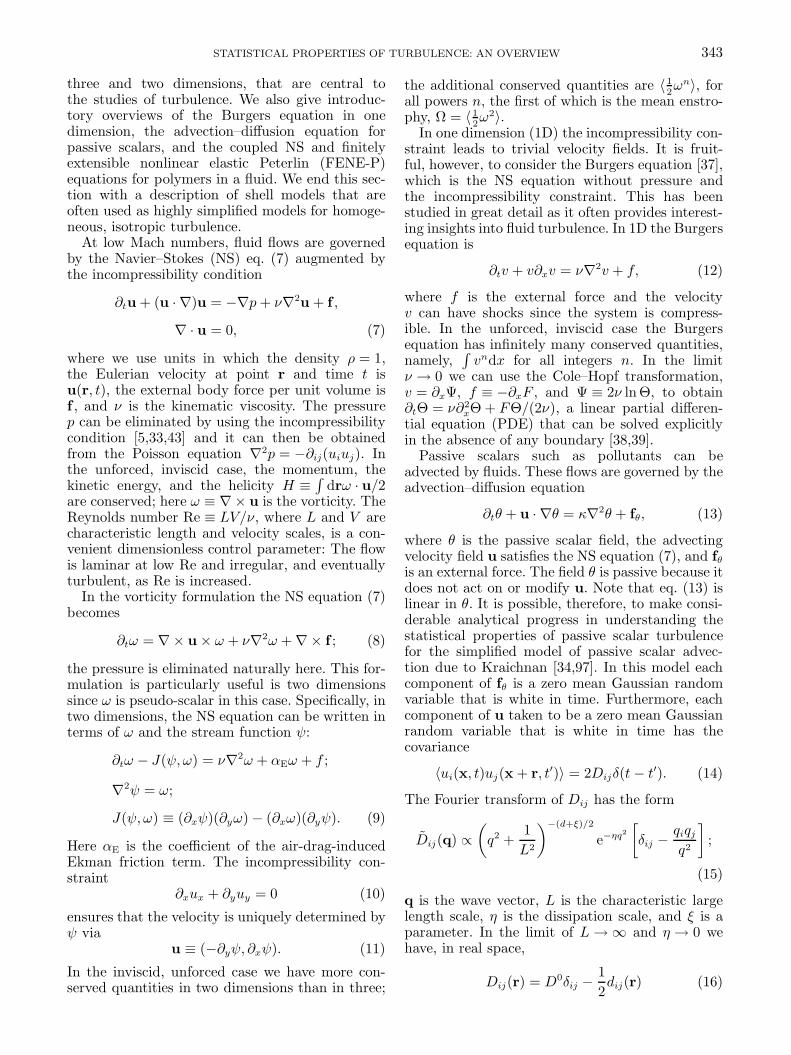
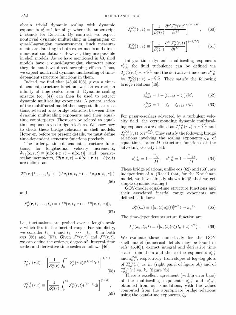
T D,up,M (r, t) ≡

[1

Sup (r)

∂MFup (r, t)∂tM

](−1/M)

, (60)

T D,θp,M (r, t) ≡

[1

Sθp(r)

∂MFθp (r, t)

∂tM

](−1/M)

. (61)

Integral-time dynamic multiscaling exponentszI,u

p,M for fluid turbulence can be defined viaT I,u

p,M(r, t) ∼ rzI,up,M and the derivative-time ones zD,u

p,M

by T D,up,M (r, t) ∼ rzD,u

p,M . They satisfy the followingbridge relations [46]:

zI,up,M = 1 + [ζp−M − ζp]/M, (62)

zD,up,M = 1 + [ζp − ζp+M ]/M. (63)

For passive-scalars advected by a turbulent velo-city field, the corresponding dynamic multiscal-ing exponents are defined as T I,θ

p,M(r, t) ∝ rzI,θp,M and

T D,θp,M (r, t) ∝ rzD,θ

p,M . They satisfy the following bridgerelations involving the scaling exponents ζM ofequal-time, order-M structure functions of theadvecting velocity field:

zI,θp,M = 1 − ζM

M, zD,θ

p,M = 1 − ζ−M

M. (64)

These bridge relations, unlike eqs (62) and (63), areindependent of p. (Recall that, for the Kraichnanmodel, we have already shown in §5 that we getsimple dynamic scaling.)

GOY-model equal-time structure functions andtheir associated inertial range exponents aredefined as follows:

Sup (kn) ≡

⟨[un(t)u∗

n(t)]p/2⟩∼ k−ζp

n . (65)

The time-dependent structure function are

F up (kn, t0, t) ≡

⟨[un(t0)u∗

n(t0 + t)]p/2⟩. (66)

We evaluate these numerically for the GOYshell model (numerical details may be found inrefs [45,46]), extract integral and derivative timescales from them and thence the exponents zI,u

p,1

and zD,up,2 , respectively, from slopes of log–log plots

of T I,up,1 (n) vs. kn (right panel of figure 6b) and of

TD,up,2 (n) vs. kn (figure 7b).There is excellent agreement (within error bars)

of the multiscaling exponents zI,up,1 and zD,u

p,2 ,obtained from our simulations, with the valuescomputed from the appropriate bridge relationsusing the equal-time exponents, ζp.


Figure 6. (a) A representative plot of the normalized fourth-order time-dependent structure function vs. the dimensionlesstime τ obtained from the GOY shell model. The plots are for shells 4, 6, and 8 (from top to bottom). (b) A log–log plot of

T I,u4,1 (n) vs. kn (for convenience, we have dropped the subscript n in the label of the x-axis in the figure); a linear fit gives

the dynamic mulstiscaling exponent zI,u4,1 .

Figure 7. (a) A representative plot of the normalized sixth-order time-dependent structure function vs. the dimensionlesstime τ obtained from the GOY shell model. The plots are for shells 4, 6, and 8 (from top to bottom). (b) A log–log plot of

T D,u6,2 (n) vs. kn (for convenience, we have dropped the subscript n in the label of the x-axis in the figure); a linear fit gives

the dynamic multiscaling exponent zD,u6,2 .

For the passive-scalar case, the equal-timeorder-p structure functions is

Sθp(kn) ≡

⟨[θ(t)θ∗n(t)]p/2

⟩∼ k

−ζθp

n (67)

and its time-dependent version is

F θp (kn, t0, t) = 〈[θn(t0)θ∗n(t0 + t)]p/2〉. (68)

We consider decaying turbulence here with t0a time origin. It is useful now to work withthe normalized time-dependent structure function,Qθ

p(n, t0, t) = F θp (kn, t0, t)/F θ

p (kn, t, 0). For the caseof passive-scalars advected by a velocity field whichis turbulent (a solution of the GOY model), wecalculate the integral (for M = 1) and derivativetime-scales (for M = 2) corresponding to eq. (58)and eq. (60), respectively. The slope of a log–logplot of T I,θ

p,1 (n) vs. kn yields the integral time-scale

exponent, zI,θp,1 , since T I,θ

p,1 (n) ∝ k−zI,θ

p,1n . Likewise,

from plots of the derivative time-scales we extractthe exponent zD,θ

p,2 . For a detailed discussion ondynamic multiscaling in this model we refer thereader to refs [46,109].

6.3 2D Navier–Stokes turbulence

We now consider illustrative numerical calcula-tions for the 2D NS equations (9)–(11). We beginwith periodic boundary conditions for which wecan use a pseudo-spectral method similar to theone given in the previous subsection for the 3DNS case. We study decaying turbulence first withthe source function f (the z component of thecurl of some force ∇×F) set to 0. We use 10242

collocation points and the standard 2/3 dealiasingprocedure; for time marching we use a second-orderRunge–Kutta scheme [113]. Our initial condition|ω(k)|2 = k−3 exp(−k2) leads to a forward cascade.We seed the flow with Lagrangian tracers and use acubic spline interpolation method to calculate their


0 0.5 1 1.5 2 2.5 3−10

−8

−6

−4

−2

0

2

log k

log

k3 E(k

)

(a)

Figure 8. (a) A log–log plot of the compensated energy spectrum k3E(k) vs. k from our DNS, of resolution 10242 , oftwo-dimensional decaying turbulence with periodic boundary conditions. The flat region indicates a scaling form E(k) ∼ k−3.(b) The trajectory of a single Lagrangian particle over a time of order 100 in a two-dimensional flow with drag and forcing.The starting point of the trajectory is in the middle of the box and is indicated by a red circle; the end point is indicatedby a blue star. The trajectory is superimposed on a pseudocolour plot of the vorticity field corresponding to the time atthe end of the Lagrangian trajectory. The figure corresponds to a forced DNS of resolution 10242 with periodic boundaryconditions, statistical steady state, and with a coefficient of Ekman friction αE = 0.1.

trajectories [122]. Representative plots from ourDNS are shown in figure 8. The first part (figure 8a)shows a compensated energy spectrum k3E(k) forthe case with no Ekman friction. Figure 8(b), froma DNS with Ekman friction αE = 0.1, Kolmogorovforcing [89], and periodic boundary conditions,shows a trajectory of a Lagrangian tracer super-imposed on a pseudocolour plot of the vorticityfield at time t = 100; the tracer starts at thepoint marked with a circle (t = 0) and ends atthe star (t = 100). For a state-of-the-art simula-tion that resolves both forward and inverse cas-cades in a forced DNS of 2D turbulence, we referthe reader to ref. [123]. Such DNS studies havealso investigated the scaling properties of struc-ture functions and have provided some evidence forconformal invariance in the inverse cascade inertialrange [124].

We end with an illustrative example of a recentDNS study [89] that sheds light on the effectof Ekman friction on the statistics of the for-ward cascade in wall-bounded flows that aredirectly relevant to laboratory soap-film experi-ments [125–128]. The details of this DNS are givenin ref. [89]. In brief, ω is driven to a statisti-cal steady state by a deterministic Kolmogorovforcing Fω ≡ kinjF0 cos(kinjx), with F0 the ampli-tude and kinj the wavenumber on which the forceacts; no-slip and no-penetration boundary condi-tions are imposed on the walls. The important non-dimensional control parameters are the Grashofnumber G = 2π||Fω||2/(k3

injρν2) and the non-

dimensional Ekman friction γ = αE/(k2injν), where

we non-dimensionalize Fω by 2π/(kinj ||Fω||2), with||Fω||2 ≡ (

∫A|Fω|2dx)1/2 and the length- and time-

scales are made non-dimensional by scaling xby k−1

inj and t by k−2inj/ν. We use a fourth-order

Runge–Kutta scheme for time marching andevaluate spatial derivatives via second-order andfourth-order, centred, finite differences, respec-tively, for points adjacent to the walls and forpoints inside the domain. The Poisson equation issolved by using a fast-Poisson solver [113] and ωis calculated at the boundaries by using Thom’sformula [89].

Since Kolmogorov forcing is inhomogeneous,we use the decomposition ψ = 〈ψ〉 + ψ′ and ω =〈ω〉 + ω′, where the angular brackets denotes atime average and the prime denotes the fluctuatingpart to calculate the order-p velocity and vorticitystructure functions. Since this is a wall-boundedflow, it is important to extract the isotropic partsof these structure functions [89,129]. Furthermore,given our resolution (20492), it becomes neces-sary to use the ESS procedure to extract exponentratios. Illustrative log–log ESS plots for velocity,Sp(R), and vorticity, Sω

p (R), structure functionsare shown in the left and right panels, respec-tively, of figure 9; their slopes yield the expo-nent ratios that are plotted vs. the order p infigure 10. The Kraichnan–Leith–Batchelor (KLB)predictions [75] for these exponent ratios, namely,ζKLB

p /ζKLB2 ∼ rp/2 and ζω,KLB

p /ζω,KLB2 ∼ r0, agree

with our values for ζp/ζ2 but not ζωp /ζ

ω2 : velo-

city structure functions do not display multiscal-ing (left panel of figure 10) whereas their vorticityanalogs do (note the curvature of the plot in theright panel of figure 10). Similar results have beenseen in DNS studies with periodic boundary condi-tions [123,130]. Additional results for PDFs of sev-eral properties can be obtained from our DNS [89];these are in striking agreement with experimentalresults [126].


Figure 9. (Left) Log–log ESS plots of the isotropic parts of the order-p velocity structure functions Sp(R) vs. S2(R);p = 3 (purple line with dots), p = 4 (red line with square), p = 5 (green line with triangles), and p = 6 (blue line withcircles). According to the KLB prediction Sp(R) ∼ Rζ

p. (Right) Log–log ESS plots of the isotropic parts of the order-pvorticity structure functions Sp(R) vs. S2(R); p = 3 (purple line with stars), p = 4 (red line with square), p = 5 (green linewith triangles), and p = 6 (blue line with circles).

Figure 10. (Left) Plots of the exponent ratios ζp/ζ2 vs. p for the velocity differences. (Right) Plots of the exponent ratiosζω

p /ζω2 vs. p for the vorticity differences.

6.4 The one-dimensional Burgers equation

In this subsection we present a few representa-tive numerical studies of the 1D Burgers equation.The first of these uses a pseudospectral methodwith 214 collocation points, the 2/3 dealising rule,and a fourth-order Runge–Kutta time-marchingscheme. In the second study of a stochasticallyforced Burgers equation (see below) we use afast-Legendre method that yields results in the zeroviscosity limit [131].

For the Burgers equation with no externalforcing and sufficiently well-behaved initial condi-tions, the velocity field develops shocks, or jumpdiscontinuities, which merge into each other withtime. The time at which the first shock appears isusually denoted by t∗. For all times greater than t∗,it is possible to calculate, analytically, the scalingexponents ζp for the equal-time structure functionsvia Sp ≡ 〈[u(x + r, t) − u(x)]p〉 ∼ Cp|r|p +C ′

p|r|,where the first term comes from the ramp, and thesecond term comes from the probability of havinga shock in the interval |r|. As a consequence of thiswe have bifractal scaling: for 0 < p < 1 the firstterm dominates leading to ζp = p and for p > 1 thesecond one dominates giving ζp = 1. This leads toan energy spectrum E(k) ∼ k−2. Representative

plots from our pseudospectral DNS, with ν = 10−3

and an initial condition u(x) = sin(x) (for whicht∗ = 1) are shown in figure 11; the left panel showsplots of the velocity field at times t = 0, 1, andt = 1.5 and the right panel the energy spectrum att = 1.

The stochastically forced Burgers equation hasplayed an important role in renormalization groupstudies [131]. In particular, consider a Gaussianrandom force f(x, t) with zero mean and the follow-ing covariance in Fourier space:

〈f(k1, t1)f(k2, t2)〉 = 2D0|k|βδ(t1 − t2)δ(k1 + k2).

(69)

Here f(k, t) is the spatial Fourier transform off(x, t), D0 is a constant, and the scaling proper-ties of the forcing is governed by the exponent β.For positive values of β, the Burgers equation canbe studied by using renormalization-group tech-niques; specifically, for β = 2 one recovers simple(Kardar–Parisi–Zhang or KPZ) scaling with theequal time exponent ζp = p. It was hoped thatforcing with negative values of β (in particularβ = −1), which cannot be studied by renormaliza-tion group methods, might yield multiscaling ofvelocity structure functions.


0 1 2 3 4 5 6−1

−0.8

−0.6

−0.4

−0.2

0

0.2

0.4

0.6

0.8

1

x

u(x)

0 0.5 1 1.5 2 2.5 3 3.5 4−25

−20

−15

−10

−5

0

log k

log E(k)

Figure 11. (Left) Snapshots of the solution of the Burgers equation obtained from our DNS with initial conditionu(x) =sin x at times t = 0 (blue), t = 1 (black) and t = 2 (red). (Right) A representative log–log plot of E(k) vs k, at timet = 1 for the Burgers equation with initial conditions u(x) = sin x.

0 0.2 0.4 0.6 0.8 1−6

−4

−2

0

2

4

6

x/2π

u(x/2

π),f(x/2

π)

0 1 2 3 4 50

0.2

0.4

0.6

0.8

1

p

ζ p

Figure 12. (Left) A snapshot of the velocity field (jagged line in blue) in steady state and the force in red fromour fast Legendre method DNS of the stochastically forced Burgers equation. (Right) A representative plot of the expo-nents ζp, with error bars, for the equal time velocity structure functions of the stochastically forced Burgers equa-tion. Bifractal scaling is shown by the black solid line and the deviations from this are believed to arise from artefacts(see text).

However, our high-resolution study [131], whichuses a fast-Legendre method, has shown that theapparent multiscaling of structure functions in thisstochastic model might arise because of numeri-cal artifacts. The general consensus is that thisstochastically forced Burgers model should showbifractal scaling. In figure 12 we present represen-tative plots of the velocity field (left panel, bluecurve) and the scaling exponents (right panel) forthis model. We have obtained the data for thesefigures by using a fast Legendre method with 218

collocation points.Numerical studies of the Burgers equation have

also proved useful in elucidating bottleneck struc-tures in energy spectra [132,133] (cf. the spec-trum in the left panel of figure 5). It turnsout that such a bottleneck does not occur inthe conventional Burgers equation. However, itdoes [134] occur in the hyperviscous one, in whichusual Laplacian dissipation operator is replacedby its αth power; this is known as hyperviscos-ity for α > 1. We show a representative compen-sated energy spectrum for the case α = 4 in the

left panel of figure 13. We have obtained thisfrom a pseudospectral DNS with 212 collocationpoints. The α→ ∞ limit is very interesting toosince, in this limit, the hyperviscous Burgers equa-tion maps on to the Galerkin-truncated versionof the inviscid Burgers equation. In this Galerkin-truncated inviscid case, the Fourier modes thermal-ize [135,136]; in a compensated energy spectrumthis shows up as E(k) ∼ k2, for large k (see theright panel of figure 13 for the case α = 200). Suchthermalization effects in the Galerkin-truncatedEuler equation have also attracted a lot of atten-tion [137], and the link between bottlenecks andthermalization has been explored in our recentwork [134] to which we refer the interestedreader.

6.5 Turbulence with polymer additives

In this subsection, we present a few resultsfrom our numerical study [138] of the analoguedrag reduction by polymer additives in homo-geneous, isotropic turbulence. This requires aDNS of considerably greater complexity than


100

101

102

103

10−6

10−5

10−4

10−3

10−2

log k

log k2E(k)

100

101

102

103

10−3

10−2

10−1

100

101

log k

log E(k)

Figure 13. (Left) A representative log–log plot of a bottleneck in the compensated energy spectrum k2E(k) of a hyper-viscous Burgers equation with α = 4. (Right) A representative log–log plot of k2E(k) vs. k for α = 200 at time t = 30. Wesee clear signatures of thermalization at large k (see text).

Figure 14. Constant-|ω| isosurfaces for |ω| = 〈|ω|〉+σ at cascade completion without and (right) with polymers (c = 0.4);〈|ω|〉 is the mean and σ the standard deviation of |ω|.

Figure 15. (Left) PDF of ω at cascade completion without (c = 0) and with polymers (c = 0.4). Note that regionsof large vorticity are reduced on the addition of polymers. (Right) Representative plots of the energy spectra Ep,m(k) orEf,m(k) vs. k for c = 0.1 (blue dashed line) and c = 0.4 (solid line).

the ones we have described above. A naivepseudospectral method cannot be used for theFENE-P model given in eqs (18) and (19):the polymer conformation tensor C is symmet-ric and positive definite. However, in a practicalimplementation of the pseudospectral method it

loses this property. We have employed a numericaltechnique that uses a Cholesky decomposition toovercome this problem, we refer the reader toref. [138] for these details.

Our recent DNS of this model has shown thatthe natural analogue drag reduction in decaying,


homogeneous, isotropic turbulence is dissipationreduction; the percentage reduction DR can bedefined as

DR ≡(εf,m − εp,m

εf,m

)

× 100. (70)

Here the superscripts f and p stand, respectively,for the fluid without and with polymers and thesuperscript m indicates the time tm at which thecascade is completed. The dependence of DR onthe polymer concentration parameter c and theWeissenberg number may be found in ref. [138].Here we show how the addition of polymers reducessmall-scale structures in the turbulent flow. Bya comparison of the isosurfaces of |ω| in the left(without polymers) and right (with polymers) pan-els of figure 14, we see that slender vorticity fil-aments are suppressed by the polymers. This isin qualitative agreement with experiments [93].The PDFs of |ω|, with and without polymers (leftpanel of figure 15) confirm that regions of largevorticity are reduced by polymers. The right panelof figure 15 shows how the polymers modify theenergy spectrum in the dissipation range. Thisbehaviour has been seen in recent experiments [96],which study the second-order structure functionthat is related simply to the energy spectrum. Fora full discussion of these and related results, werefer the reader to refs [101,138].

7. Conclusions

Turbulence provides us with a variety of challeng-ing problems. We have tried to give an overview ofsome of these, especially those that deal with thestatistical properties of turbulence. The choice oftopics has been influenced, of course, by the areasin which we have carried out research. For com-plementary, recent overviews we refer the readerto refs [1–3]; we hope the other reviews and booksthat we have cited to will provide the reader withfurther details.

Acknowledgements

We would like to thank CSIR, DST, and UGC(India) for support, and SERC (IISc) for compu-tational resources.

References

[1] Ecke R 2005 Los Alamos Science 29 124.[2] Falkovich G and Sreenivasan K R 2006 Phys. Today

59 43.

[3] Procaccia I and Sreenivasan K R 2008 Physica D2372167 and references therein.

[4] Reynolds A J 1974 Turbulent flows in engineering(New York: John Wiley).

[5] Pope S B 2000 Turbulent flows (Cambridge, UK:Cambridge University).

[6] Doering C 2009 Annu. Rev. Fluid Mech. 41 109.[7] Fefferman C 2000 Existence and smoothness of the

Navier–Stokes equation. Clay Millenium Prize Prob-lem Description.http://www.claymath.org/millennium/Navier-Stokes−Equations/Official−Problem−Description.pdf.

[8] Constantin P and Foias C 1988 Navier–Stokes equa-tions (Chicago: University of Chicago Press).

[9] Doering C and Gibbon J 1995 Applied analysis of theNavier–Stokes equations (Cambridge, UK: CambridgeUniversity Press).

[10] Majda A J and Bertozzi A L 2001 Vorticity andincompressible flow (Cambridge, UK: CambridgeUniversity Press).

[11] Tennekes H and Lumley J L 1972 A first course inturbulence (Cambridge, Massachusetts: MIT Press).

[12] Lesieur M 2008 Turbulence in fluids (The Nether-lands: Springer).

[13] Davidson P A 2007 Turbulence: An introduction forscientists and engineers (Oxford: Oxford UniversityPress).

[14] Canuto V M and Christensen-Dalsgaard J 1998 Annu.Rev. Fluid Mech. 30 167; 2003 Turbulence and mag-netic fields in astrophysics edited by Falgarone E andPassot T (New York: Springer).Miesch M S and Toomre J 2009 Annu. Rev. FluidMech. 41 317.

[15] Rai Choudhuri A 1998 The physics of fluids and plas-mas: An introduction for astrophysicists (Cambridge,UK: Cambridge University Press).

[16] Krishan V 1999 Astrophysical plasmas and fluids(Dordrecht: Kluwer).

[17] Goedbloed H and Poedts S 2004 Principles of magne-tohydrodynamics with applications to laboratory andastrophysical plasmas (Cambridge, UK: CambridgeUniversity Press).

[18] Monin A S 1983 Russ. Math. Surv. 38 127.Bradshaw P and Woods J D 1978 in Turbulence editedby P Bradshaw (New York: Springer).Majda A J and Wang X 2006 Nonlinear dynam-ics and statistical theories of basic geophysical flows(Cambridge, UK: Cambridge University Press).

[19] Boer G and Shepherd T 1983 J. Atmos. Sci. 40 164.[20] Shaw R A 2003 Annu. Rev. Fluid Mech. 35 183.[21] Biskamp D 2003 Magnetohydrodynamic turbulence

(Cambridge, UK: Cambridge University Press).[22] Verma M K 2004 Phys. Rep. 401 229.[23] Orszag S 1977 In: Fluid dynamics, Les Houches edited

by Balian R and Peube J (New York: Gordon andBreach) pp. 237–374.

[24] Rose H and Sulem P 1978 J. Phys. France 39 441.[25] Dominicis C D and Martin P 1979 Phys. Rev. A19

419.[26] Yakhot V and Orszag S 1986 Phys. Rev. Lett. 57 1722.[27] McComb W D 1991 The physics of fluid turbulence

(Oxford: Oxford University Press).[28] Eyink G L 1994 Phys. Fluids A6 3063.

Eyink G L and Goldenfeld N 1994 Phys. Rev. E504679.

[29] Bohr T, Jensen M H, Paladin G and Vulpiani A1998 Dynamical systems approach to turbulence(Cambridge, UK: Cambridge University Press).


[30] Ts Adzhemyan L, Antonov N V and Vasiliev A N1999 The field theoretic renormalization group in fullydeveloped turbulence (Gordon and Breach).

[31] Bhattacharjee J K and Bhattacharyya S 2007Nonlinear dynamics near and far from equilibrium(New Delhi: Hindustan Book Agency) Ch. 8,pp. 231–274.

[32] Non-equilibrium statistical mechanics and turbu-lence edited by Nazarenko S and Zaboronski O V(Cambridge, UK: Cambridge University Press, 2008).

[33] Frisch U 1996 Turbulence: The legacy ofA N Kolmogorov (Cambridge, UK: CambridgeUniversity Press).

[34] Falkovich G, Gawedzki K and Vergassola M 2001 Rev.Mod. Phys. 73 913.

[35] Tabeling P 2002 Phys. Rep. 362 1.[36] Kellay H and Goldburg W 2002 Rep. Prog. Phys. 65

845.[37] Burgers J M 1974 The nonlinear diffusion equation

(D Reidel: Dordrecht).[38] Frisch U and Bec J 2000 Les Houches 2000: New

trends in turbulence edited by Lesieur M (EDP-Sciences: Springer).

[39] Bec J and Khanin K 2007 Phys. Rep. 447 1.[40] Lumley J 1973 J. Polym. Sci. 7 263.[41] Procaccia I, L’vov V S and Benzi R 2008 Rev. Mod.

Phys. 80 225.[42] White C M and Mungal M G 2008 Annu. Rev. Fluid

Mech. 40 235.[43] Batchelor G K 1953 The theory of homogeneous

turbulence (Cambridge, UK: Cambridge UniversityPress).

[44] Monin A S and Yaglom A M 2007 Statistical fluidmechanics (New York: Dover) Vols 1 and 2.

[45] Pandit R, Ray S S and Mitra D 2008 Eur. Phys. J.B64 463.

[46] Ray S S, Mitra D and Pandit R 2008 New J. Phys.10 033003.

[47] Ahlers G, Grossmann S and Lohse D 2009 Rev. Mod.Phys. 81 503 and references therein.

[48] Tough J 1982 in Progress in low temperature physicsedited by D F Brewer (North-Holland, Amsterdam)Vol. VIII, p. 133.

[49] See, e.g., Cencini M, Bec J, Biferale L, Boffetta G,Celani A, Lanotte A, Musacchio S and Toschi F 2006J. Turb. 7 1.

[50] Drazin P G and Reid W H 2004 Hydrodynamic sta-bility, Second Edition (Cambridge, UK: CambridgeUniversity Press).

[51] Moehlis J, Faisst H and Eckhardt B 2004 New J.Phys. 6 56.

[52] Schlichting H and Gersten K 2006 Boundary layertheory (New Delhi: Springer).

[53] Nagib H M, Chauhan K A and Monkewitz P 2007Phil. Trans. R. Soc. A365 755.

[54] See, e.g., Barenblatt G I and Chorin A J 1998 Phys.Fluids 10 1043.Hoyas S and Jimenez J 2006 Phys. Fluids 18 011702.McKeon B J, Li J, Jiang W, Morrison J F andSmits A J 2004 J. Fluid Mech. 501 135.Smits A J and Zagarola M V 1998 Phys. Fluids 101045.Panton R L 2007 Phil. Trans. R. Soc. A365 733.L’vov V, Procaccia I and Rudenko O 2008 Phys. Rev.Lett. 100 054504 and references therein.

[55] Richardson L F 1922 Weather prediction by numericalprocess (Cambridge Univ. Press).

[56] Kolmogorov A N 1941 Dokl. Akad. Nauk SSSR 30,301; 1941 31 538.

[57] Kurian T and Fransson J H M 2007 Fluid Dyn. Res.41 021403.

[58] Mordant N, Metz P, Michel O and Pinton J-F 2001Phys. Rev. Lett. 87 214501.Mordant N, Leveque E and Pinton J-F 2004 New J.Phys. 6 116.

[59] La Porta A, Voth G A, Crawford A M, Alexander Jand Bodenschatz E 2001 Nature (London) 409 1017.Voth G A, La Porta A, Crawford A M, Alexander Jand Bodenschatz E 2002 J. Fluid Mech. 469 121.Reynolds A M, Mordant N, Crawford A M andBodenschatz E 2005 New J. Phys. 7 58.Toschi F and Bodenschatz E 2009 Annu. Rev. FluidMech. 41 375.

[60] A Arneodo et al 2008 Phys. Rev. Lett. 100 254504.[61] Kunkel G J and Marusic I 2006 J. Fluid Mech. 548

375.[62] Andreas E L, Claffey K J, Jordan R E, Fairall C W,

Guest P S, Persson P O G and Grachev A A 2006J. Fluid Mech. 559 117.

[63] Gulitski G, Kholmyansky M, Kinzelbach W, Luthi B,Tsinober A and Yorish S 2007 J. Fluid Mech. 589 57;ibid. 83; ibid. 103.

[64] Talamelli A, Persiani F, Fransson J H M,Alfredsson P H, Johansson A V, Nagib H M,Ruedi J-D, Sreenivasan K R and Monkewitz P A 2009Fluid Dyn. Res. 41 021407.

[65] Grant H L, Stewart R W and Moilliet A 1968 J. FluidMech. 12 241; Marine turbulence: Theories, obser-vations, and models Baumert H Z, Simpson J Hand Sundermann J 2005 (Cambridge, UK: CambridgeUniversity Press).

[66] Tavoularis S 2005 Measurement in fluid mechanics(Cambridge, UK: Cambridge University Press).

[67] See, e.g., Mckeon B J et al 2007 in Springerhandbook of experimental fluid mechanics edited byTropea C, Yarin A L and Foss J F (Berlin: Springer)pp. 215–471.

[68] See, e.g., Vukoslavcevic P V, Beratlis N, Balaras E,Wallace J M and Sun O 2009 Exp. Fluids 46 109.

[69] See, e.g., Elsinga G E, Scarano F, Wieneke B andvan Oudheusden B W 2006 Exp. Fluids 41 933.

[70] See, e.g.,Tao B, Katz J and Meneveau C 2000 Phys.Fluids 12 941.

[71] See, e.g., Sheng J, Malkiel E and Katz J 2008 Exp.Fluids 45 1023.

[72] Van Dyke M 1988 An album of fluid motion (Stanford,California: The Parabolic Press); see also the Galleryof fluid motionhttp://pof.aip.org/pof/gallery/index1.jsp

[73] Brown G L and Roshko A 1974 J. Fluid Mech. 64 775.[74] Kraichnan R H and Montgomery D 1980 Rep. Prog.

Phys. 43 547.[75] Kraichnan R 1967 Phys. Fluids 10 1417.

Leith C 1968 Phys. Fluids 11 671.Batchelor G 1969 Phys. Fluids Suppl. II 12 233.

[76] Douady S, Couder Y and Brachet M E 1991 Phys.Rev. Lett. 67 983.

[77] Mouri H and Hori A 2009 Fluid Dyn. Res. 41 021402.[78] Meneveau C and Sreenivasan K R 1991 J. Fluid Mech.

224 429.[79] Isihara T, Gotoh T and Kaneda Y 2009 Annu. Rev.

Fluid Mech. 41 165.[80] Kalelkar C 2005 Phys. Rev. E72 056307.


[81] Anselmet F, Gagne Y, Hopfinnger E and Antonia R1984 J. Fluid Mech. 140 63.

[82] She Z-S and Leveque E 1994 Phys. Rev. Lett. 72 336.

[83] Sreenivasan K R and Antonia R A 1997 Annu. Rev.Fluid Mech. 29 435.

[84] Praskovsky A and Oncley S 1994 Phys. Rev. Lett. 733399.

[85] Sommeria J 1986 J. Fluid Mech. 170 139.

[86] Couder Y 1984 J. Physique Lett. 45 353.

[87] Rivera M and Wu X L 2000 Phys. Rev. Lett. 85 976.Rivera M, Wu X L and Yeung C 2001 Phys. Rev. Lett.87 044501.Daniel W B and Rutgers M A 2002 Phys. Rev. Lett.89 134502.Rivera M and Ecke R 2007 arXiv:0710.5888v1.

[88] Chomaz J 2001 J. Fluid Mech. 442 387.

[89] Perlekar P and Pandit R, to be published (seehttp://arxiv.org/abs/0811.1324).

[90] Groisman A and Steinberg V 2004 New J. Phys. 6 29.

[91] Berti S, Bistagnino A, Boffetta G, Celani A andMusacchio S 2008 Phys. Rev. E77 055306(R).

[92] Toms B A 1949 in Proc. Intl. Rheological CongressHolland, 1948, p. 135.

[93] Hoyt J W 1972 Trans. ASME: J. Basic Engng. 94258.

[94] Virk P S 1975 AIChE J. 21 625.

[95] Sreenivasan K R and White C M 2000 J. Fluid Mech.409 149.

[96] Ouellette N T, Xu H and Bodenschatz E, to be pub-lished (2009); see arXiv:0708.3945.

[97] Kraichnan R 1968 Phys. Fluids 11 945; 1994 Phys.Rev. Lett. 72, 1016; 1997 Phys. Rev. Lett. 78, 4922.

[98] Vaithianathan T and Collins L 2003 J. Comput. Phys.187 1.

[99] Gledzer E 1973 Sov. Phys. Dokl. 18 216.Ohkitani K and Yamada M 1989 Prog. Theor. Phys.81 329.

[100] Wirth A and Biferale L 1996 Phys. Rev. E54 4982.Jensen M H, Paladin G and Vulpiani A 1992 Phys.Rev. A45 7214.

[101] Kalelkar C, Govindarajan R and Pandit R 2005 Phys.Rev. E72 017301.

[102] Belinicher V I and L’vov V S 1987 Sov. Phys. JETP66 303.

[103] L’vov V S, Podivilov E and Procaccia I 1997 Phys.Rev. E55 7030.

[104] Obukhov A M 1949 Izv. Akad. SSSR Serv. Geogr.Geofiz. 13 58.

[105] Corrsin S 1951 J. Appl. Phys. 22 469.[106] Stauffer D, Ferer M and Wortis M 1972 Phys. Rev.

Lett. 29 345.Aharony A 1974 Phys. Rev. B9 2107.

[107] Parisi G and Frisch U 1985 In: Turbulence andpredictability of geophysical fluid dynamics editedby Ghil M, Benzi R and Parisi G (North-Holland,Amsterdam) p. 84.

[108] Boffetta G, Mazzino A and Vulpiani A 2008 J. Phys.A: Math. Gen. 41 363001.

[109] Mitra D and Pandit R 2004 Phys. Rev. Lett. 93024501.

[110] Mitra D and Pandit R 2005 Phys. Rev. Lett. 95144501.

[111] Vincent A and Meneguzzi M 1991 J. Fluid. Mech.225 1.

[112] Canuto C, Hussaini M, Quarteroni A and Zang T 1988Spectral methods in fluid dynamics (Berlin: Spinger-Verlag).

[113] Press W, Flannery B, Teukolsky S and Vetterling W1992 Numerical recipes in Fortran (Cambridge:Cambridge University Press) pp. 848–852.

[114] Eswaran V and Pope S 1988 Comput. Fluids 16,257; the forcing is stochastic and is generated byan Ornstein-Uhlenbeck process (i.e., the noise iscoloured).

[115] Cantwell B J 1992 Phys. Fluids A4 782.[116] Kaneda Y et al 2003 Phys. Fluids 15 L21.[117] Benzi R et al 1993 Phys. Rev. E48 R29.

Dhar S, Sain A and Pandit R 1997 Phys. Rev. Lett.78 2964.

[118] Mou C Y and Weichman P B 1993 Phys. Rev. Lett.70 1101.

[119] Sain A, Manu and Pandit R 1998 Phys. Rev. Lett. 814377.

[120] Biferale L, Cencini M, Lanotte A S, Sbragaglia M andToschi F 2004 New J. Phys. 6 37.

[121] Biferale L 2003 Annu. Rev. Fluid Mech. 35 441.[122] Yeung P K 2002 Annu. Rev. Fluid Mech. 34

115.[123] Boffetta G 2007 J. Fluid Mech. 589, 253.[124] Bernard D, Boffetta G, Celani A and Falkovich G

2006 Nature Physics 2 124.Bernard D, Boffetta G, Celani A and Falkovich G2007 Phys. Rev. Lett. 98 024501.

[125] Rivera M and Wu X L 2000 Phys. Rev. Lett. 85976.

[126] Rivera M, Wu X L and Yeung C 2001 Phys. Rev. Lett.87 044501.

[127] Daniel W B and Rutgers M A 2002 Phys. Rev. Lett.89 134502.

[128] Rivera M and Ecke R 2007 arXiv:0710.5888v1.[129] Biferale L and Procaccia I 2005 Phys. Rep. 414

43.[130] Tsang Y-K, Ott E, Antonsen T M and Guzdar P N

2005 Phys. Rev. E71 066313.[131] Mitra D, Bec J, Pandit R and Frisch U 2005 Phys.

Rev. Lett. 94 194501.[132] She Z S, Doolen G, Kraichnan R H and Orszag S A

1993 Phys. Rev. Lett. 70 3251.Kaneda Y, Ishihara T, Yokokawa M, Itakura K andUno A 2003 Phys. Fluids 15 L21.Kurien S, Taylor M A and Matsumoto T 2004 Phys.Rev. E69 066313.Schumacher J 2007 Europhys. Lett. 80 54001.Mininni P D, Alexakis A and Pouquet A 2008 Phys.Rev. E77 036306.

[133] Saddoughi S G and Veeravalli S V 1994 J. Fluid Mech.268 333.As shown by Dobler W, Haugen N E L,Yousef T A and Brandenburg A 2003 Phys. Rev. E68026304.

[134] Frisch U, Kurien S, Pandit R, Pauls W, Ray S S,Wirth A and Zhu J-Z 2008 Phys. Rev. Lett. 101144501.

[135] Lee T D 1952 Quart. J. Appl. Math. 10 69.[136] Kraichnan R H 1967 Phys. Fluids 10 2080.[137] Cichowlas C, Bonaıti P, Debbasch F and Brachet M

2005 Phys. Rev. Lett. 95 264502.[138] Perlekar P, Mitra D and Pandit R 2006 Phys. Rev.

Lett. 97 264501 and to be published.

Documents

Statistical properties of turbulence: An overview · 2019-04-09 · Statistical properties of turbulence: An overview RAHUL PANDIT1,∗, PRASAD PERLEKAR and SAMRIDDHI SANKAR RAY Centre