Statistical Process Control (SPC)—the Basic

1. Introduction

The purpose of this paper is to introduce the reader to statistical process con-

trol (SPC) by showing where it fits in the area of quality management, why it is

important, and covering some of its basics. The main focus of this paper will be

the control chart which is the “heart and soul” of SPC.

This paper is organized as follows:

1.　 Introduction

2.　 Quality Management, Variation, and SPC

3.　 Types of Control Charts

4.　 Control Charts for Variables

5.　 Control Charts for Attributes

6.　 Process Capability

7.　 Other Types of Control Charts

8.　 Summary and conclusion

2. Quality Management, Variation, and SPC

The ultimate purpose of quality management is to deliver products and serv-

ices to the customer than not only satisfy but also and ideally delight the cus-

tomer. That is, products/services1) that more than meet the customer’s expecta-

tions in terms of usability, esthetics, reliability, durability, etc. To do this the

― ―91

Statistical Process Control (SPC)—The Basics

Robert B. Austenfeld, Jr.(Received on October 28, 2008)

1)　From now on the term “product” will stand for both product and service.

process(es) that create(s) the product must be good. A “good” process, in turn,

is one with little variation in terms of what it is producing—once an “ideal”

product is created it is highly desirable that the “same” product be delivered

each and every time. This means that every part of the product needs to be simi-

lar. For example if you are producing something like a gearbox where several

gears must mesh together, if each gear isn’t almost “perfect” in terms of meet-

ing some specification, the gears either will not work or will not work well and

be subject to excessive wearing due to the mismatch. Whereas if your processes

consistently produce gears well within the specification’s tolerances, your gear-

box will not only work smoothly but also last a long time due to minimal wear.

The point here is that although we can never eliminate all variation, we want to

minimize it.

The question then is how do we minimize process variation? The first thing

to understand is that there are two types of causes of variation: common and

special.2) The common causes are those that are inherent in the process itself.

They are generally random and nominally form a normal distribution. They are

due to those things than influence the process over the long term such as the

type of material being used, the capability of the machinery involved, the

ability/training of the operators, environmental conditions, etc. By changing

these factors it is possible to improve the process if such seems warranted by

the cost involved; i.e., is the process good enough or will the benefit be worth

the improvement cost?

The other source of variation is that due to special causes. These are due to

what is usually a temporary condition such as a machine getting out of adjust-

ment, a tool wearing, an input to a chemical process becoming diluted, an opera-

tor who is new and doesn’t know how to properly operate the process, or some

92― ―

Papers of the Research Society of Commerce and Economics, Vol. XLIX No. 2

2)　Sometimes called “chance” and “assignable” respectively.

temporary environmental condition such as temperature or pressure changes that

affect the process.

It is these special causes that are the main target of statistical process control

(SPC) and control charts. The purpose of a control chart is to control a process

by revealing when some significant change has occurred; i.e., when some spe-

cial cause of variation has occurred. It does this by showing when the variation

in the process causes some value being plotted on the chart—for example the

process average (or mean, denoted by the symbol for mu, m)—to go beyond a

reasonable value, usually plus or minus three standard deviations (3 sigma or,

symbolically, 3s) from that average value. Another thing of interest besides a

significant change in the process mean is whether the process’ spread3) has

changed. Since we are usually dealing with values that are essentially normally

distributed, a changed in spread will also affect the process output since what

was once considered an acceptable spread when the process was under statistical

control (i.e., no special causes present) will now cause the value of interest to go

beyond those established specification limits. Accordingly, there are usually two

charts plotted, one monitoring the process mean and the other the process spread.

3. Types of Control Charts

In general, we are dealing with two types of data: variable data from a proc-

ess that produces something where we can measure some value and attribute

data where we are concerned with whether the product of the process is defec-

tive or not, or has one or more defects. In the section that follows we will

describe in detail two types of charts for variable data:

• X-bar/R charts

• Individuals and moving range charts

― ―93

Robert B. Austenfeld, Jr.:　Statistical Process Control (SPC)—The Basics

3)　Also called “dispersion.”

And in section 5 four types of charts for attribute data will be described:

• np-chart

• p-chart

• c-chart

• u-chart

Since these are the most common charts used this will give us a basic under-

standing of control charting as the key tool for SPC. Some other types of control

charts will be very briefly described in section 7.

4. Control Charts for Variables

X-bar and R charts. The most common control charts for variables are the X-

bar ( ) and R charts. is the symbol for the sample average (mean) of the

variable X, and R stands for the sample range of the variable. The variable, of

course, is some important quality characteristic of the part being produced by

the process. As mentioned, when controlling a process we are interested in two

things: has the average shifted to some new value and has the dispersion/spread

(standard deviation) changed. If either of these things has occurred, it may mean

the process is no longer “stable and under control”—that is, producing predict-

able results. Given that we are usually working with data that is essentially nor-

mally distributed when dealing with variables, ideally the process mean will be

centered between the specification limits. Furthermore, if our process is to pro-

duce almost all of the subject parts “within spec,” the dispersion must be such

that chance of finding a sample value beyond the specification limits is almost

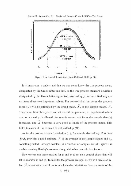
nil. For control chart purposes the value of three standard deviations is used. Fig-

ure 1 shows a normal distribution and how often a randomly selected variable

will fall within ±3 standard deviations, namely 99.7%. Section 6 of this paper

will discuss the question of whether the process can “meet the spec,” now we

are concerned only with how stable our process is.

X X

94― ―


It is important to understand that we can never know the true process mean,

designated by the Greek letter mu (m), or the true process standard deviation

designated by the Greek letter sigma (s). Accordingly, we must find ways to

estimate these two important values. For control chart purposes the process

mean (m) will be estimated by the grand mean, , of the sample means, .

The central limit theory tells us that even if the process (i.e., population) values

are not normally distributed, the sample means will be as the sample size (n)

increases, and becomes a very good estimate of the process mean. This

holds true even if n is as small as 4 (Oakland, p. 94).

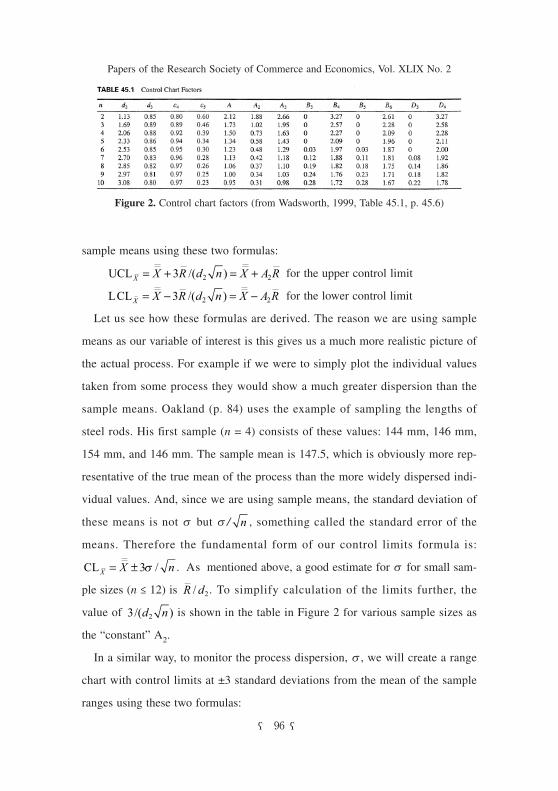
As for the process standard deviation (s), for sample sizes of say 12 or less

provides a good estimate. is the average of the sample ranges and d2,

something called Hartley’s constant, is a function of sample size (n). Figure 2 is

a table showing Hartley’s constant along with other control chart factors.

Now we can use these proxies for m and s to set up a control charts that will

let us monitor m and s . To monitor the process average, m , we will create an X-

bar ( ) chart with control limits at ±3 standard deviations from the mean of the

X X

X

R d/ 2 R

X

― ―95


Figure 1. A normal distribution (from Oakland, 2008, p. 90)

sample means using these two formulas:

for the upper control limit

for the lower control limit

Let us see how these formulas are derived. The reason we are using sample

means as our variable of interest is this gives us a much more realistic picture of

the actual process. For example if we were to simply plot the individual values

taken from some process they would show a much greater dispersion than the

sample means. Oakland (p. 84) uses the example of sampling the lengths of

steel rods. His first sample (n = 4) consists of these values: 144 mm, 146 mm,

154 mm, and 146 mm. The sample mean is 147.5, which is obviously more rep-

resentative of the true mean of the process than the more widely dispersed indi-

vidual values. And, since we are using sample means, the standard deviation of

these means is not s but s/ , something called the standard error of the

means. Therefore the fundamental form of our control limits formula is:

. As mentioned above, a good estimate for s for small sam-

ple sizes (n ≤ 12) is . To simplify calculation of the limits further, the

value of is shown in the table in Figure 2 for various sample sizes as

the “constant” A2.

In a similar way, to monitor the process dispersion, s , we will create a range

chart with control limits at ±3 standard deviations from the mean of the sample

ranges using these two formulas:

UCL /( )X X R d n X A R= + = +3 2 2

LCL /( )X X R d n X A R= − = −3 2 2

n

CL /X X n= ± 3σ

R d/ 2

3 2/( )d n

96― ―


Figure 2. Control chart factors (from Wadsworth, 1999, Table 45.1, p. 45.6)

for the upper control limit

for the lower control limit

The fundamental form of these equations is: where is our esti-

mate of the process’ mean range. To estimate the range standard deviation we

use another factor from the table in Figure 2: d3, and the relationship s R = d3s .

Again using our estimate of s , , we get s R = d3s = and the

first form of the above formulas. As with the formulas for the X-bar ( ) chart

control limits these formulas are simplified into a final form using the “con-

stants” D4 and D3, which again are read from the table in Figure 2 according to

the sample size.

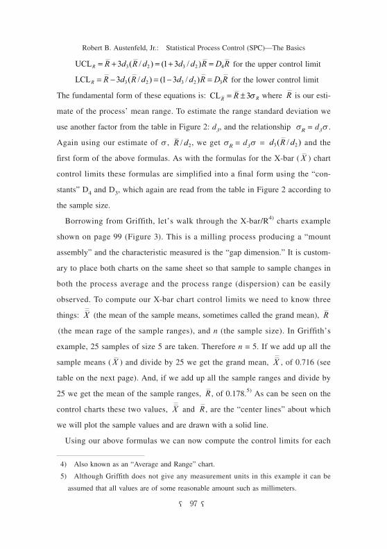
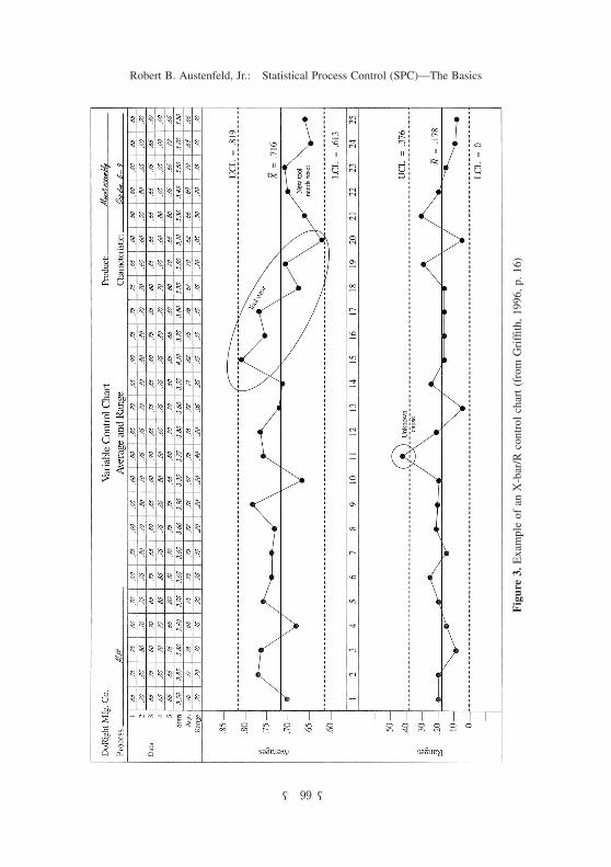
Borrowing from Griffith, let’s walk through the X-bar/R4) charts example

shown on page 99 (Figure 3). This is a milling process producing a “mount

assembly” and the characteristic measured is the “gap dimension.” It is custom-

ary to place both charts on the same sheet so that sample to sample changes in

both the process average and the process range (dispersion) can be easily

observed. To compute our X-bar chart control limits we need to know three

things: (the mean of the sample means, sometimes called the grand mean),

(the mean rage of the sample ranges), and n (the sample size). In Griffith’s

example, 25 samples of size 5 are taken. Therefore n = 5. If we add up all the

sample means ( ) and divide by 25 we get the grand mean, , of 0.716 (see

table on the next page). And, if we add up all the sample ranges and divide by

25 we get the mean of the sample ranges, , of 0.178.5) As can be seen on the

control charts these two values, and , are the “center lines” about which

we will plot the sample values and are drawn with a solid line.

Using our above formulas we can now compute the control limits for each

UCL ( / ) ( / )R R d R d d d R D R= + = + =3 1 33 2 3 2 4

LCL ( / ) ( / )R R d R d d d R D R= − = − =3 1 33 2 3 2 3

CLR RR= ± 3σ R

R d/ 2 d R d3 2( / )

X

X R

X X

R

X R

― ―97


4)　Also known as an “Average and Range” chart. 5)　Although Griffith does not give any measurement units in this example it can be assumed that all values are of some reasonable amount such as millimeters.

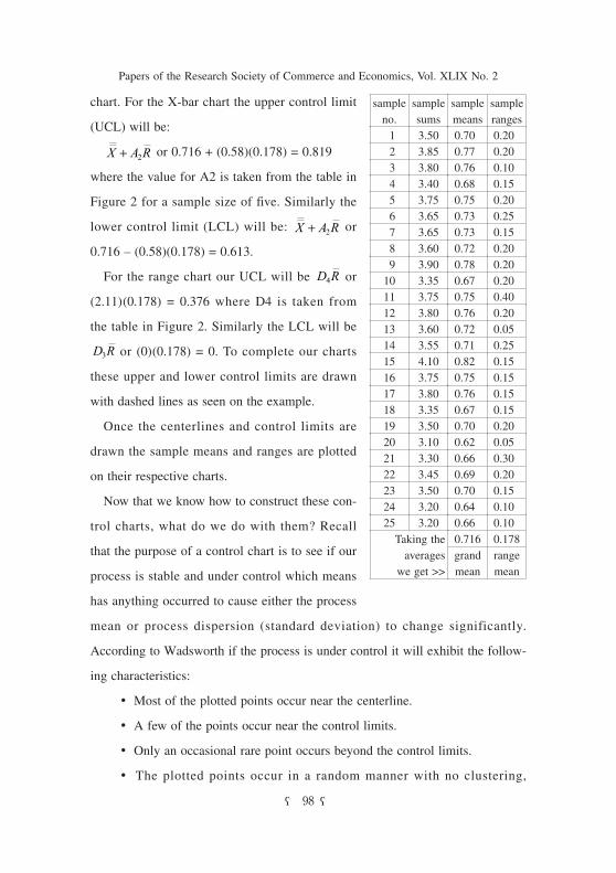
chart. For the X-bar chart the upper control limit

(UCL) will be:

or 0.716 + (0.58)(0.178) = 0.819

where the value for A2 is taken from the table in

Figure 2 for a sample size of five. Similarly the

lower control limit (LCL) will be: or

0.716 – (0.58)(0.178) = 0.613.

For the range chart our UCL will be or

(2.11)(0.178) = 0.376 where D4 is taken from

the table in Figure 2. Similarly the LCL will be

or (0)(0.178) = 0. To complete our charts

these upper and lower control limits are drawn

with dashed lines as seen on the example.

Once the centerlines and control limits are

drawn the sample means and ranges are plotted

on their respective charts.

Now that we know how to construct these con-

trol charts, what do we do with them? Recall

that the purpose of a control chart is to see if our

process is stable and under control which means

has anything occurred to cause either the process

mean or process dispersion (standard deviation) to change significantly.

According to Wadsworth if the process is under control it will exhibit the follow-

ing characteristics:

• Most of the plotted points occur near the centerline.

• A few of the points occur near the control limits.

• Only an occasional rare point occurs beyond the control limits.

• The plotted points occur in a random manner with no clustering,

X A R+ 2

X A R+ 2

D R4

D R3

98― ―


sample ranges

sample means

sample sums

sample no.

0.20 0.70 3.50 10.20 0.77 3.85 20.10 0.76 3.80 30.15 0.68 3.40 40.20 0.75 3.75 50.25 0.73 3.65 60.15 0.73 3.65 70.20 0.72 3.60 80.20 0.78 3.90 90.20 0.67 3.35100.40 0.75 3.75110.20 0.76 3.80120.05 0.72 3.60130.25 0.71 3.55140.15 0.82 4.10150.15 0.75 3.75160.15 0.76 3.80170.15 0.67 3.35180.20 0.70 3.50190.05 0.62 3.10200.30 0.66 3.30210.20 0.69 3.45220.15 0.70 3.50230.10 0.64 3.20240.10 0.66 3.20250.1780.716Taking the

averages we get >>

range mean

grand mean

― ―99


Figure 3. Example of an X-bar/R control chart (from Griffith, 1996, p. 16)

trending, or other departure from a random distribution. (p. 45.7)

Should any of these characteristics not be present it means there is a good

chance the process is not in control and we have a special cause of variation. In

our Griffith example we can see a typical instance where Wadsworth’s fourth

characteristic is “violated” starting with sample number 15. There is a down-

ward trend that would suggest that something is causing the process to no longer

exhibit randomness. In this case it is traced to “tool wear.” Note the comment at

sample number 11 of “unknown cause” for the point falling beyond the range

chart’s UCL. Since this seems to be an isolated instance it may simply be that

“occasional rare point” mentioned in Wadsworth’s third characteristic. However,

since the chance of that occurring is so small it should be investigated. Appar-

ently in this case nothing was found to be amiss.

Griffith states that any indication of an out-of-control condition “deserves

some action to find the special cause and eliminate it” and “[i]f the cause is

found and eliminated, recalculate the control limits (p. 17).” He further recom-

mends a fairly frequent recalculation of the control limits in any event to be sure

they accurately reflect the actual current process that could, in fact, be changing.

Griffith also emphasizes the importance of marking anything of significance on

the chart so it becomes a running record of the process. Examples of this are

shown on the Griffith control chart.

There are many other “rules” for interpreting this type of control chart and the

reader is referred to the Griffith, Wadsworth, Oakland and other references. As a

matter of interest, Oakland writes from a UK/European perspective and

describes control charts in terms of not only upper and lower control limits set

at three standard deviations but an additional set of control limits set at two stan-

dard deviations. The former are called “action lines” and the latter “warning

lines.” The idea is to give a more precise way of detecting possible problems

with the addition of the warning lines.

100― ―


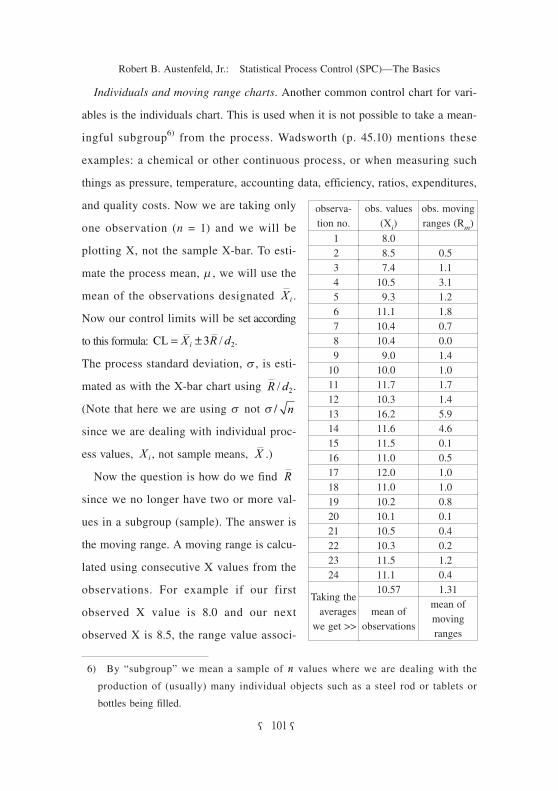
Individuals and moving range charts. Another common control chart for vari-

ables is the individuals chart. This is used when it is not possible to take a mean-

ingful subgroup6) from the process. Wadsworth (p. 45.10) mentions these

examples: a chemical or other continuous process, or when measuring such

things as pressure, temperature, accounting data, efficiency, ratios, expenditures,

and quality costs. Now we are taking only

one observation (n = 1) and we will be

plotting X, not the sample X-bar. To esti-

mate the process mean, m , we will use the

mean of the observations designated .

Now our control limits will be set according

to this formula: .

The process standard deviation, s , is esti-

mated as with the X-bar chart using .

(Note that here we are using s not s/

since we are dealing with individual proc-

ess values, , not sample means, .)

Now the question is how do we find

since we no longer have two or more val-

ues in a subgroup (sample). The answer is

the moving range. A moving range is calcu-

lated using consecutive X values from the

observations. For example if our first

observed X value is 8.0 and our next

observed X is 8.5, the range value associ-

Xi

CL /= ±X R di 3 2

R d/ 2

n

Xi X

R

― ―101


6)　By “subgroup” we mean a sample of n values where we are dealing with the production of (usually) many individual objects such as a steel rod or tablets or

bottles being filled.

obs. moving ranges (Rm)

obs. values(Xi)

observation no.

8.0 10.5 8.5 21.1 7.4 33.1 10.5 41.2 9.3 51.8 11.1 60.7 10.4 70.0 10.4 81.4 9.0 91.0 10.0 101.7 11.7 111.4 10.3 125.9 16.2 134.6 11.6 140.1 11.5 150.5 11.0 161.0 12.0 171.0 11.0 180.8 10.2 190.1 10.1 200.4 10.5 210.2 10.3 221.2 11.5 230.4 11.1 241.3110.57

Taking the averages we get >>

mean of moving ranges

mean of observations

ated with the “8.5” observation will be 0.5. Note there will always be k-1 range

values, where k is the number of observations. Taking the average of the mov-

ing ranges, , we get and use this for our . This is also used to calcu-

late our control limits for our moving range chart in the same way we did that

for the previous range chart; i.e., and .

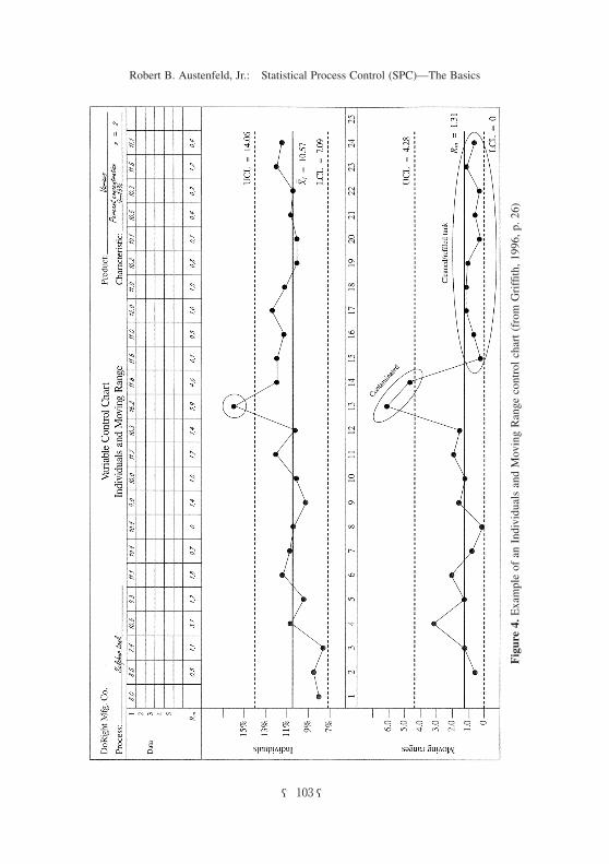
Again drawing on a Griffith example as shown on the next page (Figure 4),

let’s calculate the control limits. For the observed values as listed in the table on

the previous page we calculate the mean of the individual X values, , and the

mean of the moving ranges, . These respectively are 10.57 and 1.31. Using

the above formulas our UCL is 10.57 + 3(1.31)/1.13 (for n = 2) equals 10.57 +

3.48 or 14.05.7) And our LCL is 10.57 − 3.48 or 7.09. Similarly for the moving

range chart: UCL is 3.27(1.31) equals 4.28 and the LCL is 0(1.31) equals zero.

As with Griffith’s X-bar/R chart example this individuals/moving range chart

shows examples of problems that a control chart might typically reveal such as

contamination at observation 13 and how cleaning the tank improved things from

sample 15 on.

5. Control Charts for Attributes

Introduction. So far we have been talking about control charts for variables,

that is for processes where we measure some variable quality characteristic such

as the diameter of a shaft or the number of tablets being placed in a container or

the amount of liquid being put in a bottle. There are also processes where the

question is does this product meet some stated standard to make it acceptable or

not. Once the standard has been clearly established, we will use our control

chart to determine how many of those parts or products actually have met the

standard. Oakland (p. 192) gives these examples:

Rm Rm R R

UCL = D Rm4 LCL = D Rm3

Xi

R

102― ―


7)　The control chart (Figure 4) shows 14.06, perhaps due to “rounding error.”

― ―103


Figure 4. Example of an Individuals and Moving Range control chart (from Griffith, 1996, p. 26)

…bubbles in a windscreen [windshield], the general appearance of a paint

surface, accidents, the particles of contamination in a sample of polymer,

clerical errors in an invoice and the number of telephone calls.

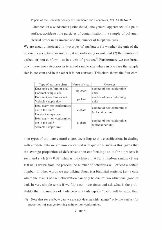
We are usually interested in two types of attributes: (1) whether the unit of the

product is acceptable or not, i.e., it is conforming or not, and (2) the number of

defects or non-conformities in a unit of product.8) Furthermore we can break

down these two categories in terms of sample size where in one case the sample

size is constant and in the other it is not constant. This chart shows the four com-

mon types of attribute control charts according to this classification. In dealing

with attribute data we are now concerned with questions such as this: given that

the average proportion of defectives (non-conforming) units for a process is

such and such (say 0.02) what is the chance that for a random sample of say

100 units drawn from the process the number of defectives will exceed a certain

number. In other words we are talking about is a binomial statistic; i.e., a case

where the results of each observation can only be one of two situations: good or

bad. In very simple terms if we flip a coin two times and ask what is the prob-

ability that the number of tails (where a tails equals “bad”) will be more than

104― ―


MeasuresName of chartType of attribute chartnumber of non-conformingunits

np-chartDoes unit conform or not?Constant sample size.

number of non-conformingunits

p-chartDoes unit conform or not?Variable sample size.

number of non-conformities(defects) per unit.

c-chartHow many non-conformities are in the unit?Constant sample size.

number of non-conformities(defects) per unit.

u-chartHow many non-conformities are in the unit?Variable sample size.

8)　Note that for attribute data we are not dealing with “ranges” only the number (or proportion) of non-conforming units or non-conformities.

one. For this to happen both flips would have to be a tails, and the probability

of that is only 0.25 if we have a “fair” coin. If we were to repeat this experi-

ment several times and keep getting two tails we would suspect the coin is no

longer fair and that the “average proportion of defectives” for the process has

changed from 0.5 to some much higher value. Let’s now go through an exam-

ple, this time from Oakland, and see how these ideas apply for an np-chart.

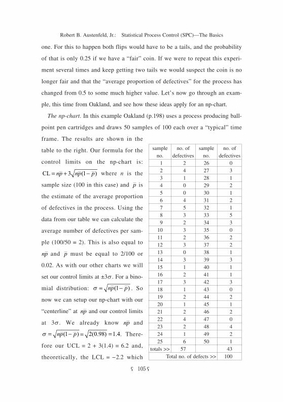
The np-chart. In this example Oakland (p.198) uses a process producing ball-

point pen cartridges and draws 50 samples of 100 each over a “typical” time

frame. The results are shown in the

table to the right. Our formula for the

control limits on the np-chart is:

where n is the

sample size (100 in this case) and is

the estimate of the average proportion

of defectives in the process. Using the

data from our table we can calculate the

average number of defectives per sam-

ple (100/50 = 2). This is also equal to

and must be equal to 2/100 or

0.02. As with our other charts we will

set our control limits at ±3s . For a bino-

mial distribution: . So

now we can setup our np-chart with our

“centerline” at and our control limits

at 3s . We already know and

= . There-

fore our UCL = 2 + 3(1.4) = 6.2 and,

theoretically, the LCL = −2.2 which

CL ( )= + −np np p3 1

p

np p

σ = −np p( )1

np

np

σ = −np p( )1 2 0 98 1 4( . ) .=

― ―105


no. of defectives

sample no.

no. of defectives

sample no.

026 2 1 327 4 2 128 1 3 229 0 4 130 0 5 231 4 6 132 5 7 533 3 8 334 2 9 035 310 236 211 237 312 138 013 339 314 140 115 141 216 342 317 043 118 244 219 145 120 246 221 047 422 448 223 249 124 150 6254357totals >>100 Total no. of defects >>

makes no sense so is set to zero. To quote Oakland:

In control charts for attributes it is commonly found that only the upper

limits are specified since we wish to detect an increase in defectives.

Lower control lines may be useful, however, to indicate when a significant

process improvement has occurred, or to indicate when suspicious results

have been plotted. (p. 201)

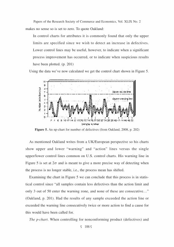
Using the data we’ve now calculated we get the control chart shown in Figure 5.

As mentioned Oakland writes from a UK/European perspective so his charts

show upper and lower “warning” and “action” lines versus the single

upper/lower control lines common on U.S. control charts. His warning line in

Figure 5 is set at 2s and is meant to give a more precise way of detecting when

the process is no longer stable, i.e., the process mean has shifted.

Examining the chart in Figure 5 we can conclude that this process is in statis-

tical control since “all samples contain less defectives than the action limit and

only 3 out of 50 enter the warning zone, and none of these are consecutive…”

(Oakland, p. 201). Had the results of any sample exceeded the action line or

exceeded the warning line consecutively twice or more action to find a cause for

this would have been called for.

The p-chart. When controlling for nonconforming product (defectives) and

106― ―


Figure 5. An np-chart for number of defectives (from Oakland, 2008, p. 202)

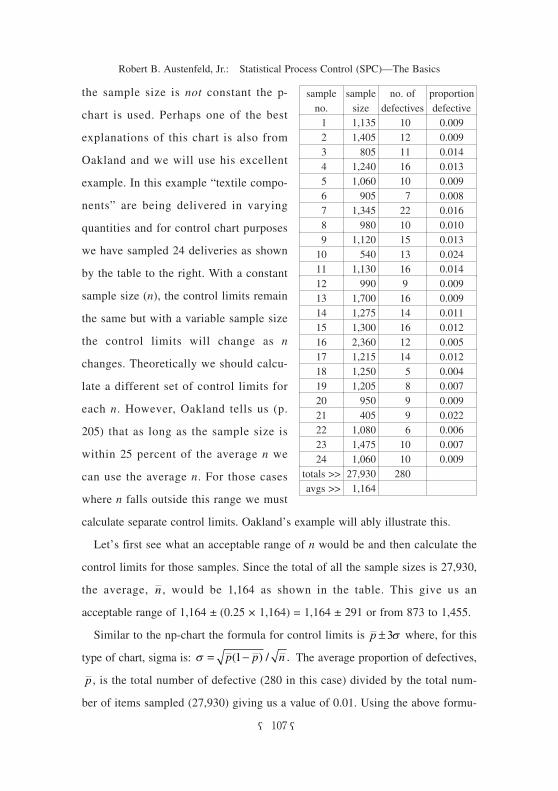
the sample size is not constant the p-

chart is used. Perhaps one of the best

explanations of this chart is also from

Oakland and we will use his excellent

example. In this example “textile compo-

nents” are being delivered in varying

quantities and for control chart purposes

we have sampled 24 deliveries as shown

by the table to the right. With a constant

sample size (n), the control limits remain

the same but with a variable sample size

the control limits will change as n

changes. Theoretically we should calcu-

late a different set of control limits for

each n. However, Oakland tells us (p.

205) that as long as the sample size is

within 25 percent of the average n we

can use the average n. For those cases

where n falls outside this range we must

calculate separate control limits. Oakland’s example will ably illustrate this.

Let’s first see what an acceptable range of n would be and then calculate the

control limits for those samples. Since the total of all the sample sizes is 27,930,

the average, , would be 1,164 as shown in the table. This give us an

acceptable range of 1,164 ± (0.25 × 1,164) = 1,164 ± 291 or from 873 to 1,455.

Similar to the np-chart the formula for control limits is where, for this

type of chart, sigma is: The average proportion of defectives,

, is the total number of defective (280 in this case) divided by the total num-

ber of items sampled (27,930) giving us a value of 0.01. Using the above formu-

n

p ± 3σ

σ = −p p n( ) / .1

p

― ―107


proportion defective

no. of defectives

sample size

sample no.

0.009 101,135 10.009 121,405 20.014 11805 30.013 161,240 40.009 101,060 50.008 7905 60.016 221,345 70.010 10980 80.013 151,120 90.024 13540100.014 161,130110.009 9990120.009 161,700130.011 141,275140.012 161,300150.005 122,360160.012 141,215170.004 51,250180.007 81,205190.009 9950200.022 9405210.006 61,080220.007 101,475230.009 101,06024

28027,930totals >>1,164avgs >>

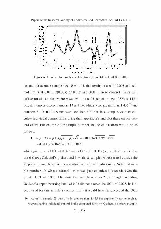
las and our average sample size, = 1164, this results in a s of 0.003 and con-

trol limits at 0.01 ± 3(0.003) or 0.019 and 0.001. These control limits will

suffice for all samples where n was within the 25 percent range of 873 to 1455;

i.e., all samples except numbers 13 and 16, which were greater than 1,455,9) and

numbers 3, 10 and 21, which were less than 873. For these samples we must cal-

culate individual control limits using their specific n’s and plot these on our con-

trol chart. For example for sample number 10 the calculation would be as

follows:

which gives us an UCL of 0.023 and a LCL of −0.003 (or, in effect, zero). Fig-

ure 6 shows Oakland’s p-chart and how those samples whose n fell outside the

25 percent range have had their control limits drawn individually. Note that sam-

ple number 10, whose control limits we just calculated, exceeds even the

greater UCL of 0.023. Also note that sample number 21, although exceeding

Oakland’s upper “warning line” of 0.02 did not exceed the UCL of 0.025, had

been used for this sample’s control limits it would have far exceeded the UCL

n

CL ( ) / . . /= ± = ± − = ±p p p p n3 3 1 0 01 3 0 0099 540σ

= ± = ±0 01 3 0 0043 0 01 0 013. ( . ) . .

n

108― ―


9)　Actually sample 23 was a little greater than 1,455 but apparently not enough to warrant having individual control limits computed for it on Oakland’s p-chart example.

Figure 6. A p-chart for number of defectives (from Oakland, 2008, p. 208)

of 0.019 indicating a potentially serious problem.

Analyzing this chart, Oakland (p. 206) notes that all is reasonably well until

delivery of sample number 10 which probably resulted in some discussions

between the supplier and the customer bringing the quality back to within accept-

able levels until another possible problem occurred as indicated by the results of

sample number 21.

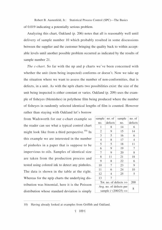
The c-chart. So far with the np and p charts we’ve been concerned with

whether the unit (item being inspected) conforms or doesn’t. Now we take up

the situation where we want to assess the number of non-conformities, that is

defects, in a unit. As with the np/n charts two possibilities exist: the size of the

unit being inspected is either constant or varies. Oakland (p. 209) uses the exam-

ple of fisheyes (blemishes) in polythene film being produced where the number

of fisheyes in randomly selected identical lengths of film is counted. However

rather than staying with Oakland let’s borrow

from Wadsworth for our c-chart example so

the reader can see what a typical control chart

might look like from a third perspective.10) In

this example we are interested in the number

of pinholes in a paper that is suppose to be

impervious to oils. Samples of identical size

are taken from the production process and

tested using colored ink to detect any pinholes.

The data is shown in the table at the right.

Whereas for the np/p charts the underlying dis-

tribution was binomial, here it is the Poisson

distribution whose standard deviation is simply

― ―109


10)　Having already looked at examples from Griffith and Oakland.

no. of defects

sample no.

no. of defects

sample no.

614 8 11415 9 2 616 5 3 417 8 41118 5 5 719 9 6 820 9 7182111 8 622 8 9 923 7101024 611 525 412

713200Tot. no. of defects >>

8Avg. no. of defects per sample c (200/25) >>

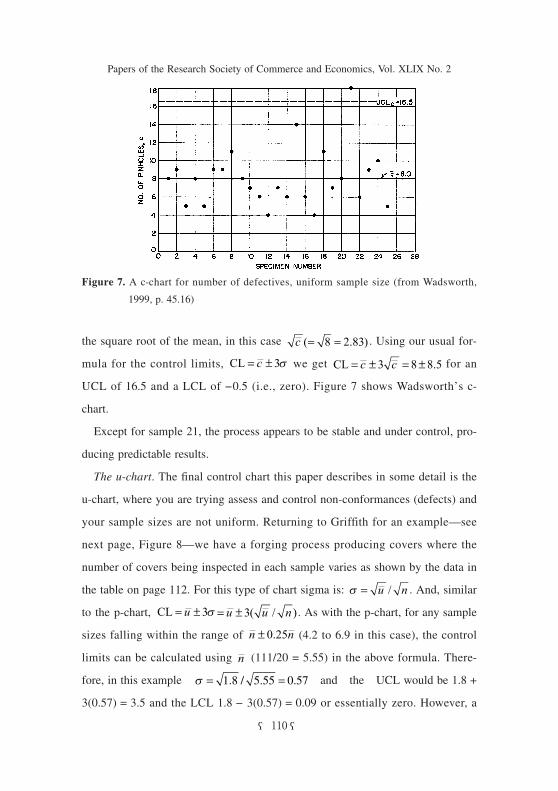
the square root of the mean, in this case . Using our usual for-

mula for the control limits, we get for an

UCL of 16.5 and a LCL of −0.5 (i.e., zero). Figure 7 shows Wadsworth’s c-

chart.

Except for sample 21, the process appears to be stable and under control, pro-

ducing predictable results.

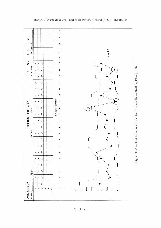
The u-chart. The final control chart this paper describes in some detail is the

u-chart, where you are trying assess and control non-conformances (defects) and

your sample sizes are not uniform. Returning to Griffith for an example—see

next page, Figure 8—we have a forging process producing covers where the

number of covers being inspected in each sample varies as shown by the data in

the table on page 112. For this type of chart sigma is: . And, similar

to the p-chart, . As with the p-chart, for any sample

sizes falling within the range of (4.2 to 6.9 in this case), the control

limits can be calculated using (111/20 = 5.55) in the above formula. There-

fore, in this example and the UCL would be 1.8 +

3(0.57) = 3.5 and the LCL 1.8 − 3(0.57) = 0.09 or essentially zero. However, a

c ( . )= =8 2 83

CL = ±c 3σ CL .= ± = ±c c3 8 8 5

σ = u n/

CL = ±u 3σ = ±u u n3( / )

n n± 0 25.

n

σ = =1 8 5 55 0 57. / . .

110― ―


Figure 7. A c-chart for number of defectives, uniform sample size (from Wadsworth,

1999, p. 45.16)

― ―111


Figure 8. A u-chart for number of defectives/unit (from Griffith, 1996, p. 83)

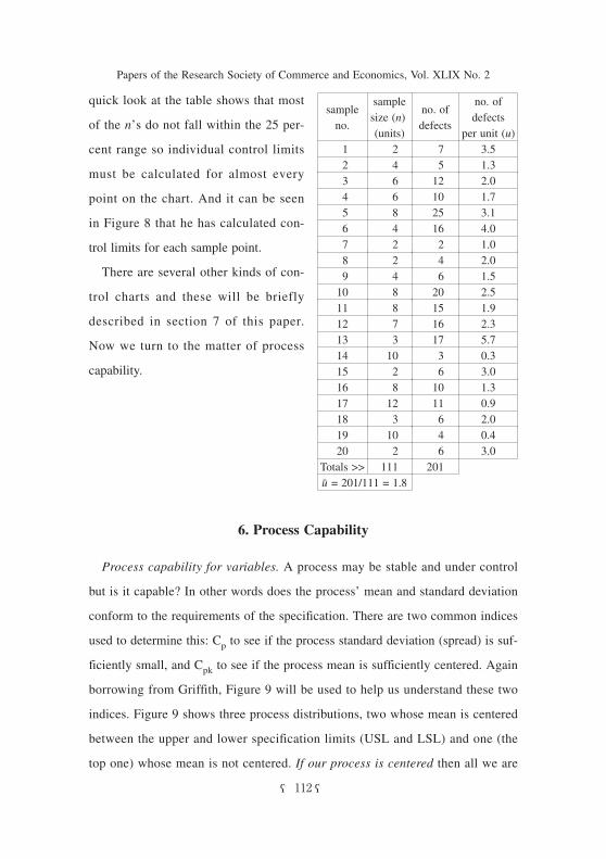
quick look at the table shows that most

of the n’s do not fall within the 25 per-

cent range so individual control limits

must be calculated for almost every

point on the chart. And it can be seen

in Figure 8 that he has calculated con-

trol limits for each sample point.

There are several other kinds of con-

trol charts and these will be briefly

described in section 7 of this paper.

Now we turn to the matter of process

capability.

6. Process Capability

Process capability for variables. A process may be stable and under control

but is it capable? In other words does the process’ mean and standard deviation

conform to the requirements of the specification. There are two common indices

used to determine this: Cp to see if the process standard deviation (spread) is suf-

ficiently small, and Cpk to see if the process mean is sufficiently centered. Again

borrowing from Griffith, Figure 9 will be used to help us understand these two

indices. Figure 9 shows three process distributions, two whose mean is centered

between the upper and lower specification limits (USL and LSL) and one (the

top one) whose mean is not centered. If our process is centered then all we are

112― ―


no. of defects per unit (u)

no. of defects

sample size (n) (units)

sample no.

3.5 7 2 11.3 5 4 22.0 12 6 31.7 10 6 43.1 25 8 54.0 16 4 61.0 2 2 72.0 4 2 81.5 6 4 92.5 20 8101.9 15 8112.3 16 7125.7 17 3130.3 3 10143.0 6 2151.3 10 8160.9 11 12172.0 6 3180.4 4 10193.0 6 220

201111Totals >>u = 201/111 = 1.8

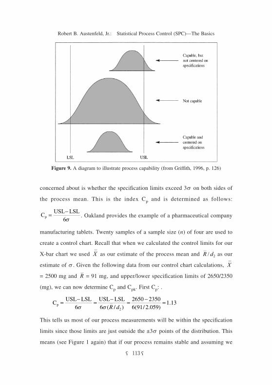
concerned about is whether the specification limits exceed 3s on both sides of

the process mean. This is the index Cp and is determined as follows:

. Oakland provides the example of a pharmaceutical company

manufacturing tablets. Twenty samples of a sample size (n) of four are used to

create a control chart. Recall that when we calculated the control limits for our

X-bar chart we used as our estimate of the process mean and as our

estimate of s. Given the following data from our control chart calculations,

= 2500 mg and = 91 mg, and upper/lower specification limits of 2650/2350

(mg), we can now determine Cp and Cpk. First Cp: .

This tells us most of our process measurements will be within the specification

limits since those limits are just outside the ±3s points of the distribution. This

means (see Figure 1 again) that if our process remains stable and assuming we

CUSL LSL

p = −6σ

X R d/ 2

X

R

CUSL LSL USL LSL

( / ) ( / . ).p = − = − = − =

6 62650 23506 91 2 059

1 132σ σ R d

― ―113


Figure 9. A diagram to illustrate process capability (from Griffith, 1996, p. 126)

do have a normal distribution at least 99.7% of our values will be “within spec.”

The problem with the Cp index is it doesn’t account for a process that is not

centered on the specification limits, hence, the Cpk index. Now it is necessary to

calculate two values: one for the USL and one for the LSL:

and . It should be apparent that if we used the same data as

before in Oakland’s tablet example we would get the same result of 1.13 since

that process was centered. To show how Cpk works Oakland changed the above

values to = 2650 mg and the upper and lower specification limits to 2750

mg and 2250 mg; there is no change in s with remaining at 91 mg. This

new data yields:

and

.

This tells us that the distance between our process mean and the upper specifica-

tion limit (USL) is less than 3s and, therefore, some of our values will be out-

side the USL and be unacceptable. It also tells us the distance between our proc-

ess mean and the LSL is very large, in fact, three times 3s so there is little

chance that any values would fall below the LSL. The top distribution in Figure

9 shows this situation.11) This process is definitely not capable. Had we com-

puted only Cp we would have gotten:

and might have concluded the process was capable.

At what value of Cpk should we consider the process as not capable? If the

specification and 3s points coincide it means that on average 99.7% of the

CUSL

pk(u) = − X3σ

CLSL

pk( )13

= −Xσ

X

R

CUSL

( / . ).pk(u) = − = − =X

3

2750 2650

3 91 2 0590 75

σ

CLSL

( / . ).pk( )1

3

2650 2250

3 91 2 0593 02= − = − =X

σ

CUSL LSL

( / . ).p = − = =

6

500

6 91 2 0591 89

σ

114― ―


11)　Although Figure 9 shows this as a “capable” process it actually would not be since too much of its distribution exceeds the USL.

measurements will be within specification and only 0.3% out of specification if

the process is centered (Cp = 1.0). If it is not centered12) but the 3s point of the

“tail” that is closest to either the upper or lower specification limit coincides

with that limit then only about 0.15% of the values will be out of specification

(Cpk = 1.0). Because we probably never have a purely normal process and proc-

esses do tend to become unstable we would want our specification limits to be

more than just 1.0 and Oakland (p. 285) recommends a Cpk of 2.0 for a “high

level of confidence in the producer”—for example, like the bottom distribution

in Figure 9. Remember, however, that measures of process capability are prem-

ised on the process being in statistical control.

If the process is not capable then the alternatives are either to relax the specifi-

cation if that is feasible or improve the process through whatever means; e.g.,

better input material, equipment, procedures, training, or, even, some entirely

new approach to producing desired product.

Process capability for attributes. Process capability for attribute data is sim-

ply the process average given the process remains in statistical control. For ex-

ample for the p-chart the process capability will be 1.00 minus , the average

proportion of defectives. So if = 0.02 the process capability will be 0.98

meaning the process is theorectically capable of producing 98% good product.

As can be seen by now control charts and process capability go hand in hand

and provide the basis for not only controlling existing processes but for carrying

out the most basic dictum of quality management; i.e., continuous improvement

of the processes.

p

p

― ―115


12)　There are times when the measurement in question is the time it takes to do something, like process an insurance claim or carry out some transaction. Here we are

only concerned with one side of the distribution where the process values are less

than some desired standard.

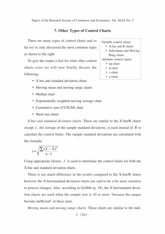
7. Other Types of Control Charts

There are many types of control charts and so

far we’ve only discussed the most common types

as shown to the right:

To give the reader a feel for what other control

charts exist we will now briefly discuss the

following:

• X-bar and standard deviation charts

• Moving mean and moving range charts

• Median chart

• Exponentially weighted moving average chart

• Cumulative sum (CUSUM) chart

• Short run charts

X-bar and standard deviation charts. These are similar to the X-bar/R charts

except , the average of the sample standard deviations, is used instead of to

calculate the control limits. The sample standard deviations are calculated with

this formula:

Using appropriate factors, is used to determine the control limits for both the

X-bar and standard deviation charts.

There is not much difference in the results compared to the X-bar/R charts

however the X-bar/standard deviation charts are said to be a bit more sensitive

to process changes. Also, according to Griffith (p. 19), the X-bar/standard devia-

tion charts are used when the sample size is 10 or more “because the ranges

become inefficient” at these sizes.

Moving mean and moving range charts. These charts are similar to the indi-

s R

sX X

ni=−

−∑ ( )2

1

s

116― ―


Variable control charts:

• X-bar and R charts• Individuals and Moving Rang charts

Attribute control charts:

• np-chart• p-chart• c-chart• u-chart

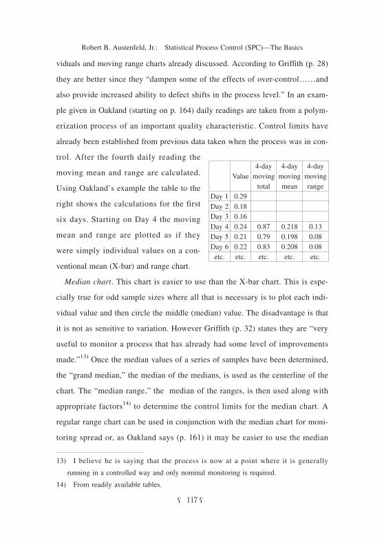
viduals and moving range charts already discussed. According to Griffith (p. 28)

they are better since they “dampen some of the effects of over-control……and

also provide increased ability to defect shifts in the process level.” In an exam-

ple given in Oakland (starting on p. 164) daily readings are taken from a polym-

erization process of an important quality characteristic. Control limits have

already been established from previous data taken when the process was in con-

trol. After the fourth daily reading the

moving mean and range are calculated.

Using Oakland’s example the table to the

right shows the calculations for the first

six days. Starting on Day 4 the moving

mean and range are plotted as if they

were simply individual values on a con-

ventional mean (X-bar) and range chart.

Median chart. This chart is easier to use than the X-bar chart. This is espe-

cially true for odd sample sizes where all that is necessary is to plot each indi-

vidual value and then circle the middle (median) value. The disadvantage is that

it is not as sensitive to variation. However Griffith (p. 32) states they are “very

useful to monitor a process that has already had some level of improvements

made.”13) Once the median values of a series of samples have been determined,

the “grand median,” the median of the medians, is used as the centerline of the

chart. The “median range,” the median of the ranges, is then used along with

appropriate factors14) to determine the control limits for the median chart. A

regular range chart can be used in conjunction with the median chart for moni-

toring spread or, as Oakland says (p. 161) it may be easier to use the median

― ―117


4-day moving range

4-day moving mean

4-day moving total

Value

0.29Day 10.18Day 20.16Day 3

0.130.2180.870.24Day 40.080.1980.790.21Day 50.080.2080.830.22Day 6etc.etc.etc.etc.etc.

13)　I believe he is saying that the process is now at a point where it is generally running in a controlled way and only nominal monitoring is required.

14)　From readily available tables.

range to calculate those control limits also.

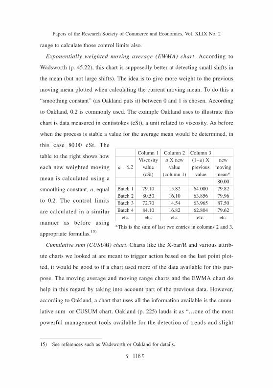
Exponentially weighted moving average (EWMA) chart. According to

Wadsworth (p. 45.22), this chart is supposedly better at detecting small shifts in

the mean (but not large shifts). The idea is to give more weight to the previous

moving mean plotted when calculating the current moving mean. To do this a

“smoothing constant” (as Oakland puts it) between 0 and 1 is chosen. According

to Oakland, 0.2 is commonly used. The example Oakland uses to illustrate this

chart is data measured in centistokes (cSt), a unit related to viscosity. As before

when the process is stable a value for the average mean would be determined, in

this case 80.00 cSt. The

table to the right shows how

each new weighted moving

mean is calculated using a

smoothing constant, a, equal

to 0.2. The control limits

are calculated in a similar

manner as before using

appropriate formulas.15)

Cumulative sum (CUSUM) chart. Charts like the X-bar/R and various attrib-

ute charts we looked at are meant to trigger action based on the last point plot-

ted, it would be good to if a chart used more of the data available for this pur-

pose. The moving average and moving range charts and the EWMA chart do

help in this regard by taking into account part of the previous data. However,

according to Oakland, a chart that uses all the information available is the cumu-

lative sum or CUSUM chart. Oakland (p. 225) lauds it as “…one of the most

powerful management tools available for the detection of trends and slight

118― ―


15)　See references such as Wadsworth or Oakland for details.

Column 3Column 2Column 1new moving mean*

(1−a) X previous value

a X new value

(column 1)

Viscosity value (cSt)

a = 0.2

80.0079.8264.00015.8279.10Batch 179.9663.85616.1080.50Batch 287.5063.96514.5472.70Batch 379.6262.80416.8284.10Batch 4etc.etc.etc.etc.etc.

*This is the sum of last two entries in columns 2 and 3.

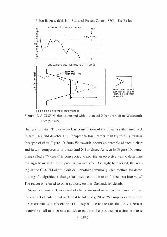
changes in data.” The drawback is construction of the chart is rather involved.

In fact, Oakland devotes a full chapter to this. Rather than try to fully explain

this type of chart Figure 10, from Wadsworth, shows an example of such a chart

and how it compares with a standard X-bar chart. As seen in Figure 10, some-

thing called a “V-mask” is constructed to provide an objective way to determine

if a significant shift in the process has occurred. As might be guessed, the scal-

ing of the CUSUM chart is critical. Another commonly used method for deter-

mining if a significant change has occurred is the use of “decision intervals.”

The reader is referred to other sources, such as Oakland, for details.

Short run charts. These control charts are used when, as the name implies,

the amount of data is not sufficient to take, say, 20 or 25 samples as we do for

the traditional X-bar/R charts. This may be due to the fact that only a certain

relatively small number of a particular part is to be produced at a time or due to

― ―119


Figure 10. A CUSUM chart compared with a standard X-bar chart (from Wadsworth,

1999, p. 45.19)

a the process cycling so fast the production run is over before the data needed

can be gathered. Various short run charts have been devised to permit control of

these process for both variable data and attribute data. A key feature of these

types of charts is the use of coded data based on some target value. The reader

is referred to other sources for the details of constructing short run charts.

Griffith discusses this type of chart in considerable detail for both variable and

attribute data.

Concluding remarks. As mentioned, there are many different types of control

charts to accommodate various situations or the need for more sensitivity to

process changes. This section has touched on a some of the more common ones.

Examples of others not mentioned here include the mid-range, multivariate, and

the Box-Jenkins Manual Adjustment charts.

8. Summary and Conclusion

The purpose of this paper has been to provide an introductory look at statisti-

cal process control (SPC) concentrating mainly on control charts since they are

at the heart of the matter. Several common types of control charts have been

described in detail, two for variable data and four for attribute data. Some other

types of control charts have also been briefly described in section 7. There is

much, much more to SPC than given here such as more detail on how to inter-

pret these charts and, even before that, how to judiciously select the

variable/attribute to be charted. Perhaps the most important thing to remember is

that control charts are not meant for controlling some quality characteristic but

rather for controlling the process and, by virtue of that, making sure the charac-

teristic being measured (and others inherent in the part/product) remains within

desired values. In fact, control charts should be considered as a means to go

beyond simply maintaining a “status quo” and as a tool for getting to know the

process better and better and learning of ways to improve it!

120― ―


References

Oakland, J. S. (2008). Statistical Process Control (6th edition). Oxford: Elsevier.

Griffith, G. K. (1996). Statistical Process Control for Long and Short Runs (2nd edition).

Milwaukee: ASQC Quality Press.

Wadsworth, H. M. (1999). Section 45, Statistical Process Control. In J. M. Juran (Ed.),

Juran’s Quality Control Handbook, 5th ed. New York: McGraw-Hill.

― ―121


Documents

Statistical Process Control (SPC)—the Basic