Preprint typeset in JHEP style - HYPER VERSION Lent Term, 2011 and 2012

Statistical PhysicsUniversity of Cambridge Part II Mathematical Tripos

Dr David Tong

Department of Applied Mathematics and Theoretical Physics,

Centre for Mathematical Sciences,

Wilberforce Road,

Cambridge, CB3 OBA, UK

http://www.damtp.cam.ac.uk/user/tong/statphys.html

d.tong@damtp.cam.ac.uk

– 1 –

Recommended Books and Resources

• Reif, Fundamentals of Statistical and Thermal Physics

A comprehensive and detailed account of the subject. It’s solid. It’s good. It isn’t

quirky.

• Kardar, Statistical Physics of Particles

A modern view on the subject which offers many insights. It’s superbly written, if a

little brief in places. A companion volume, “The Statistical Physics of Fields” covers

aspects of critical phenomena. Both are available to download as lecture notes. Links

are given on the course webpage

• Landau and Lifshitz, Statistical Physics

Russian style: terse, encyclopedic, magnificent. Much of this book comes across as

remarkably modern given that it was first published in 1958.

• Mandl, Statistical Physics

This is an easy going book with very clear explanations but doesn’t go into as much

detail as we will need for this course. If you’re struggling to understand the basics,

this is an excellent place to look. If you’re after a detailed account of more advanced

aspects, you should probably turn to one of the books above.

• Pippard, The Elements of Classical Thermodynamics

This beautiful little book walks you through the rather subtle logic of classical ther-

modynamics. It’s very well done. If Arnold Sommerfeld had read this book, he would

have understood thermodynamics the first time round.

There are many other excellent books on this subject, often with different empha-

sis. I recommend “States of Matter” by David Goodstein which covers several topics

beyond the scope of this course but offers many insights. For an entertaining yet tech-

nical account of thermodynamics that lies somewhere between a textbook and popular

science, read “The Four Laws” by Peter Atkins.

A number of good lecture notes are available on the web. Links can be found on the

course webpage: http://www.damtp.cam.ac.uk/user/tong/statphys.html

– 2 –

Contents

1. The Fundamentals of Statistical Mechanics 1

1.1 Introduction 1

1.2 The Microcanonical Ensemble 2

1.2.1 Entropy and the Second Law of Thermodynamics 5

1.2.2 Temperature 8

1.2.3 An Example: The Two State System 11

1.2.4 Pressure, Volume and the First Law of Thermodynamics 14

1.2.5 Ludwig Boltzmann (1844-1906) 16

1.3 The Canonical Ensemble 17

1.3.1 The Partition Function 18

1.3.2 Energy and Fluctuations 19

1.3.3 Entropy 22

1.3.4 Free Energy 25

1.4 The Chemical Potential 26

1.4.1 Grand Canonical Ensemble 27

1.4.2 Grand Canonical Potential 29

1.4.3 Extensive and Intensive Quantities 29

1.4.4 Josiah Willard Gibbs (1839-1903) 30

2. Classical Gases 31

2.1 The Classical Partition Function 31

2.1.1 From Quantum to Classical 32

2.2 Ideal Gas 33

2.2.1 Equipartition of Energy 36

2.2.2 The Sociological Meaning of Boltzmann’s Constant 36

2.2.3 Entropy and Gibbs’s Paradox 38

2.2.4 The Ideal Gas in the Grand Canonical Ensemble 39

2.3 Maxwell Distribution 40

2.3.1 A History of Kinetic Theory 42

2.4 Diatomic Gas 44

2.5 Interacting Gas 47

2.5.1 The Mayer f Function and the Second Virial Coefficient 49

2.5.2 van der Waals Equation of State 51

2.5.3 The Cluster Expansion 54

2.6 Screening and the Debye-Huckel Model of a Plasma 59

3. Quantum Gases 61

3.1 Density of States 61

3.1.1 Relativistic Systems 62

3.2 Photons: Blackbody Radiation 63

3.2.1 Planck Distribution 65

3.2.2 The Cosmic Microwave Background Radiation 67

3.2.3 The Birth of Quantum Mechanics 68

3.2.4 Max Planck (1858-1947) 69

3.3 Phonons 69

3.3.1 The Debye Model 69

3.4 The Diatomic Gas Revisited 74

3.5 Bosons 76

3.5.1 Bose-Einstein Distribution 77

3.5.2 A High Temperature Quantum Gas is (Almost) Classical 80

3.5.3 Bose-Einstein Condensation 81

3.5.4 Heat Capacity: Our First Look at a Phase Transition 85

3.6 Fermions 89

3.6.1 Ideal Fermi Gas 90

3.6.2 Degenerate Fermi Gas and the Fermi Surface 91

3.6.3 The Fermi Gas at Low Temperature 92

3.6.4 A More Rigorous Approach: The Sommerfeld Expansion 96

3.6.5 White Dwarfs and the Chandrasekhar limit 99

3.6.6 Pauli Paramagnetism 101

3.6.7 Landau Diamagnetism 103

4. Classical Thermodynamics 107

4.1 Temperature and the Zeroth Law 108

4.2 The First Law 110

4.3 The Second Law 112

4.3.1 The Carnot Cycle 114

4.3.2 Thermodynamic Temperature Scale and the Ideal Gas 116

4.3.3 Entropy 119

4.3.4 Adiabatic Surfaces 122

4.3.5 A History of Thermodynamics 125

4.4 Thermodynamic Potentials: Free Energies and Enthalpy 127

4.4.1 Enthalpy 130

– 1 –

4.4.2 Maxwell’s Relations 130

4.5 The Third Law 132

5. Phase Transitions 134

5.1 Liquid-Gas Transition 134

5.1.1 Phase Equilibrium 136

5.1.2 The Clausius-Clapeyron Equation 139

5.1.3 The Critical Point 141

5.2 The Ising Model 146

5.2.1 Mean Field Theory 148

5.2.2 Critical Exponents 151

5.2.3 Validity of Mean Field Theory 153

5.3 Some Exact Results for the Ising Model 154

5.3.1 The Ising Model in d = 1 Dimensions 155

5.3.2 2d Ising Model: Low Temperatures and Peierls Droplets 156

5.3.3 2d Ising Model: High Temperatures 161

5.3.4 Kramers-Wannier Duality 164

5.4 Landau Theory 169

5.4.1 Second Order Phase Transitions 171

5.4.2 First Order Phase Transitions 174

5.4.3 Lee-Yang Zeros 175

5.5 Landau-Ginzburg Theory 179

5.5.1 Correlations 181

5.5.2 Fluctuations 182

– 2 –

Acknowledgements

These lecture notes are far from original. They borrow heavily both from the books

described above and the online resources listed on the course webpage. I benefited a lot

from the lectures by Mehran Kardar and by Chetan Nayak. This course is built on the

foundation of previous courses given in Cambridge by Ron Horgan and Matt Wingate.

I am also grateful to Ray Goldstein for help in developing the present syllabus. I am

supported by the Royal Society and Alex Considine.

– 3 –

1. The Fundamentals of Statistical Mechanics

“Ludwig Boltzmann, who spent much of his life studying statistical mechan-

ics, died in 1906 by his own hand. Paul Ehrenfest, carrying on the work,

died similarly in 1933. Now it is our turn to study statistical mechanics.”

David Goodstein

1.1 Introduction

Statistical mechanics is the art of turning the microscopic laws of physics into a de-

scription of Nature on a macroscopic scale.

Suppose you’ve got theoretical physics cracked. Suppose you know all the funda-

mental laws of Nature, the properties of the elementary particles and the forces at play

between them. How can you turn this knowledge into an understanding of the world

around us? More concretely, if I give you a box containing 1023 particles and tell you

their mass, their charge, their interactions, and so on, what can you tell me about the

stuff in the box?

There’s one strategy that definitely won’t work: writing down the Schrodinger equa-

tion for 1023 particles and solving it. That’s typically not possible for 23 particles,

let alone 1023. What’s more, even if you could find the wavefunction of the system,

what would you do with it? The positions of individual particles are of little interest

to anyone. We want answers to much more basic, almost childish, questions about the

contents of the box. Is it wet? Is it hot? What colour is it? Is the box in danger of

exploding? What happens if we squeeze it, pull it, heat it up? How can we begin to

answer these kind of questions starting from the fundamental laws of physics?

The purpose of this course is to introduce the dictionary that allows you translate

from the microscopic world where the laws of Nature are written to the everyday

macroscopic world that we’re familiar with. This will allow us to begin to address very

basic questions about how matter behaves.

We’ll see many examples. For centuries — from the 1600s to the 1900s — scientists

were discovering “laws of physics” that govern different substances. There are many

hundreds of these laws, mostly named after their discovers. Boyle’s law and Charles’s

law relate pressure, volume and temperature of gases (they are usually combined into

the ideal gas law); the Stefan-Boltzmann law tells you how much energy a hot object

emits; Wien’s displacement law tells you the colour of that hot object; the Dulong-Petit

– 1 –

law tells you how much energy it takes to heat up a lump of stuff; Curie’s law tells

you how a magnet loses its magic if you put it over a flame; and so on and so on. Yet

we now know that these laws aren’t fundamental. In some cases they follow simply

from Newtonian mechanics and a dose of statistical thinking. In other cases, we need

to throw quantum mechanics into the mix as well. But in all cases, we’re going to see

how derive them from first principles.

A large part of this course will be devoted to figuring out the interesting things

that happen when you throw 1023 particles together. One of the recurring themes will

be that 1023 6= 1. More is different: there are key concepts that are not visible in

the underlying laws of physics but emerge only when we consider a large collection of

particles. One very simple example is temperature. This is not a fundamental concept:

it doesn’t make sense to talk about the temperature of a single electron. But it would

be impossible to talk about physics of the everyday world around us without mention

of temperature. This illustrates the fact that the language needed to describe physics

on one scale is very different from that needed on other scales. We’ll see several similar

emergent quantities in this course, including the phenomenon of phase transitions where

the smooth continuous laws of physics conspire to give abrupt, discontinuous changes

in the structure of matter.

Historically, the techniques of statistical mechanics proved to be a crucial tool for

understanding the deeper laws of physics. Not only is the development of the subject

intimately tied with the first evidence for the existence of atoms, but quantum me-

chanics itself was discovered by applying statistical methods to decipher the spectrum

of light emitted from hot objects. (We will study this derivation in Section 3). How-

ever, physics is not a finished subject. There are many important systems in Nature –

from high temperature superconductors to black holes – which are not yet understood

at a fundamental level. The information that we have about these systems concerns

their macroscopic properties and our goal is to use these scant clues to deconstruct the

underlying mechanisms at work. The tools that we will develop in this course will be

crucial in this task.

1.2 The Microcanonical Ensemble

“Anyone who wants to analyze the properties of matter in a real problem

might want to start by writing down the fundamental equations and then

try to solve them mathematically. Although there are people who try to

use such an approach, these people are the failures in this field. . . ”

Richard Feynman, sugar coating it.

– 2 –

We’ll start by considering an isolated system with fixed energy, E. For the purposes

of the discussion we will describe our system using the language of quantum mechanics,

although we should keep in mind that nearly everything applies equally well to classical

systems.

In your first two courses on quantum mechanics you looked only at systems with a

few degrees of freedom. These are defined by a Hamiltonian, H, and the goal is usually

to solve the time independent Schrodinger equation

H|ψ〉 = E|ψ〉

In this course, we will still look at systems that are defined by a Hamiltonian, but now

with a very large number of degrees of freedom, say N ∼ 1023. The energy eigenstates

|ψ〉 are very complicated objects since they contain information about what each of

these particles is doing. They are called microstates.

In practice, it is often extremely difficult to write down the microstate describing

all these particles. But, more importantly, it is usually totally uninteresting. The

wavefunction for a macroscopic system very rarely captures the relevant physics because

real macroscopic systems are not described by a single pure quantum state. They are

in contact with an environment, constantly buffeted and jostled by outside influences.

Each time the system is jogged slightly, it undergoes a small perturbation and there

will be a probability that it transitions to another state. If the perturbation is very

small, then the transitions will only happen to states of equal (or very nearly equal)

energy. But with 1023 particles, there can be many many microstates all with the same

energy E. To understand the physics of these systems, we don’t need to know the

intimate details of any one state. We need to know the crude details of all the states.

It would be impossibly tedious to keep track of the dynamics which leads to tran-

sitions between the different states. Instead we will resort to statistical methods. We

will describe the system in terms of a probability distribution over the quantum states.

In other words, the system is in a mixed state rather than a pure state. Since we have

fixed the energy, there will only be a non-zero probability for states which have the

specified energy E. We will denote a basis of these states as |n〉 and the probability

that the systems sits in a given state as p(n). Within this probability distribution, the

expectation value of any operator O is

〈O〉 =∑

n

p(n)〈n|O|n〉

Our immediate goal is to understand what probability distribution p(n) is appropriate

for large systems.

– 3 –

Firstly, we will greatly restrict the kind of situations that we can talk about. We will

only discuss systems that have been left alone for some time. This ensures that the

energy and momentum in the system has been redistributed among the many particles

and any memory of whatever special initial conditions the system started in has long

been lost. Operationally, this means that the probability distribution is independent

of time which ensures that the expectation values of the macroscopic observables are

also time independent. In this case, we say that the system is in equilibrium. Note that

just because the system is in equilibrium does not mean that all the components of the

system have stopped moving; a glass of water left alone will soon reach equilibrium but

the atoms inside are still flying around.

We are now in a position to state the fundamental assumption of statistical mechan-

ics. It is the idea that we should take the most simple minded approach possible and

treat all states the same. Or, more precisely:

For an isolated system in equilibrium, all accessible microstates are equally likely.

Since we know nothing else about the system, such a democratic approach seems

eminently reasonable. Notice that we’ve left ourselves a little flexibility with the in-

clusion of the word “accessible”. This refers to any state that can be reached due to

the small perturbations felt by the system. For the moment, we will take it mean all

states that have the same energy E. Later, we shall see contexts where we add further

restrictions on what it means to be an accessible state.

Let us introduce some notation. We define

Ω(E) = Number of states with energy E

The probability that the system with fixed energy E is in a given state |n〉 is simply

p(n) =1

Ω(E)(1.1)

The probability that the system is in a state with some different energy E ′ 6= E is zero.

This probability distribution, relevant for systems with fixed energy, is known as the

microcanonical ensemble. Some comments:

• Ω(E) is a usually ridiculously large number. For example, suppose that we have

N ∼ 1023 particles, each of which can only be in one of two quantum states – say

“spin up” and “spin down”. Then the total number of microstates of the system

is 21023. This is a silly number. In some sense, numbers this large can never have

– 4 –

any physical meaning! They only appear in combinatoric problems, counting

possible eventualities. They are never answers to problems which require you

to count actual existing physical objects. One, slightly facetious, way of saying

this is that numbers this large can’t have physical meaning because they are the

same no matter what units they have. (If you don’t believe me, think of 21023

as a distance scale: it is effectively the same distance regardless of whether it is

measured in microns or lightyears. Try it!).

• In quantum systems, the energy levels will be discrete. However, with many

particles the energy levels will be finely spaced and can be effectively treated as

a continuum. When we say that Ω(E) counts the number of states with energy

E we implicitly mean that it counts the number of states with energy between

E and E + δE where δE is small compared to the accuracy of our measuring

apparatus but large compared to the spacing of the levels.

• We phrased our discussion in terms of quantum systems but everything described

above readily carries over the classical case. In particular, the probabilities p(n)

have nothing to do with quantum indeterminacy. They are due entirely to our

ignorance.

1.2.1 Entropy and the Second Law of Thermodynamics

We define the entropy of the system to be

S(E) = kB log Ω(E) (1.2)

Here kB is a fundamental constant, known as Boltzmann’s constant . It has units of

Joules per Kelvin.

kB ≈ 1.381 × 10−23JK−1 (1.3)

The log in (1.2) is the natural logarithm (base e, not base 10). Why do we take the

log in the definition? One reason is that it makes the numbers less silly. While the

number of states is of order Ω ∼ eN , the entropy is merely proportional to the number

of particles in the system, S ∼ N . This also has the happy consequence that the

entropy is an additive quantity. To see this, consider two non-interacting systems with

energies E1 and E2 respectively. Then the total number of states of both systems is

Ω(E1, E2) = Ω1(E1)Ω(E2)

while the entropy for both systems is

S(E1, E2) = S1(E1) + S2(E2)

– 5 –

The Second Law

Suppose we take the two, non-interacting, systems mentioned above and we bring them

together. We’ll assume that they can exchange energy, but that the energy levels of each

individual system remain unchanged. (These are actually contradictory assumptions!

If the systems can exchange energy then there must be an interaction term in their

Hamiltonian. But such a term would shift the energy levels of each system. So what

we really mean is that these shifts are negligibly small and the only relevant effect of

the interaction is to allow the energy to move between systems).

The energy of the combined system is still Etotal = E1 + E2. But the first system

can have any energy E ≤ Etotal while the second system must have the remainder

Etotal −E. In fact, there is a slight caveat to this statement: in a quantum system we

can’t have any energy at all: only those discrete energies Ei that are eigenvalues of the

Hamiltonian. So the number of available states of the combined system is

Ω(Etotal) =∑

Ei

Ω1(Ei)Ω2(Etotal −Ei)

=∑

Ei

exp

(

S1(Ei)

kB+S2(Etotal −Ei)

kB

)

(1.4)

There is a slight subtlety in the above equation. Both system 1 and system 2 have

discrete energy levels. How do we know that if Ei is an energy of system 1 then

Etotal −Ei is an energy of system 2. In part this goes back to the comment made above

about the need for an interaction Hamiltonian that shifts the energy levels. In practice,

we will just ignore this subtlety. In fact, for most of the systems that we will discuss in

this course, the discreteness of energy levels will barely be important since they are so

finely spaced that we can treat the energy E of the first system as a continuous variable

and replace the sum by an integral. We will see many explicit examples of this in the

following sections.

At this point, we turn again to our fundamental assumption — all states are equally

likely — but now applied to the combined system. This has fixed energy Etotal so can be

thought of as sitting in the microcanonical ensemble with the distribution (1.1) which

means that the system has probability p = 1/Ω(Etotal) to be in each state. Clearly, the

entropy of the combined system is greater or equal to that of the original system,

S(Etotal) ≡ kB log Ω(Etotal) ≥ S1(E1) + S2(E2) (1.5)

which is true simply because the states of the two original systems are a subset of the

total number of possible states.

– 6 –

While (1.5) is true for any two systems, there is a useful approximation we can make

to determine S(Etotal) which holds when the number of particles, N , in the game is

very large. We have already seen that the entropy scales as S ∼ N . This means that

the expression (1.4) is a sum of exponentials of N , which is itself an exponentially large

number. Such sums are totally dominated by their maximum value. For example,

suppose that for some energy, E⋆, the exponent has a value that’s twice as large as any

other E. Then this term in the sum is larger than all the others by a factor of eN .

And that’s a very large number. All terms but the maximum are completely negligible.

(The equivalent statement for integrals is that they can be evaluated using the saddle

point method). In our case, the maximum value, E = E⋆, occurs when

∂S1(E⋆)

∂E− ∂S2(Etotal − E⋆)

∂E= 0 (1.6)

where this slightly cumbersome notation means (for the first term) ∂S1/∂E evaluated at

E = E⋆. The total entropy of the combined system can then be very well approximated

by

S(Etotal) ≈ S1(E⋆) + S2(Etotal −E⋆) ≥ S1(E1) + S2(E2)

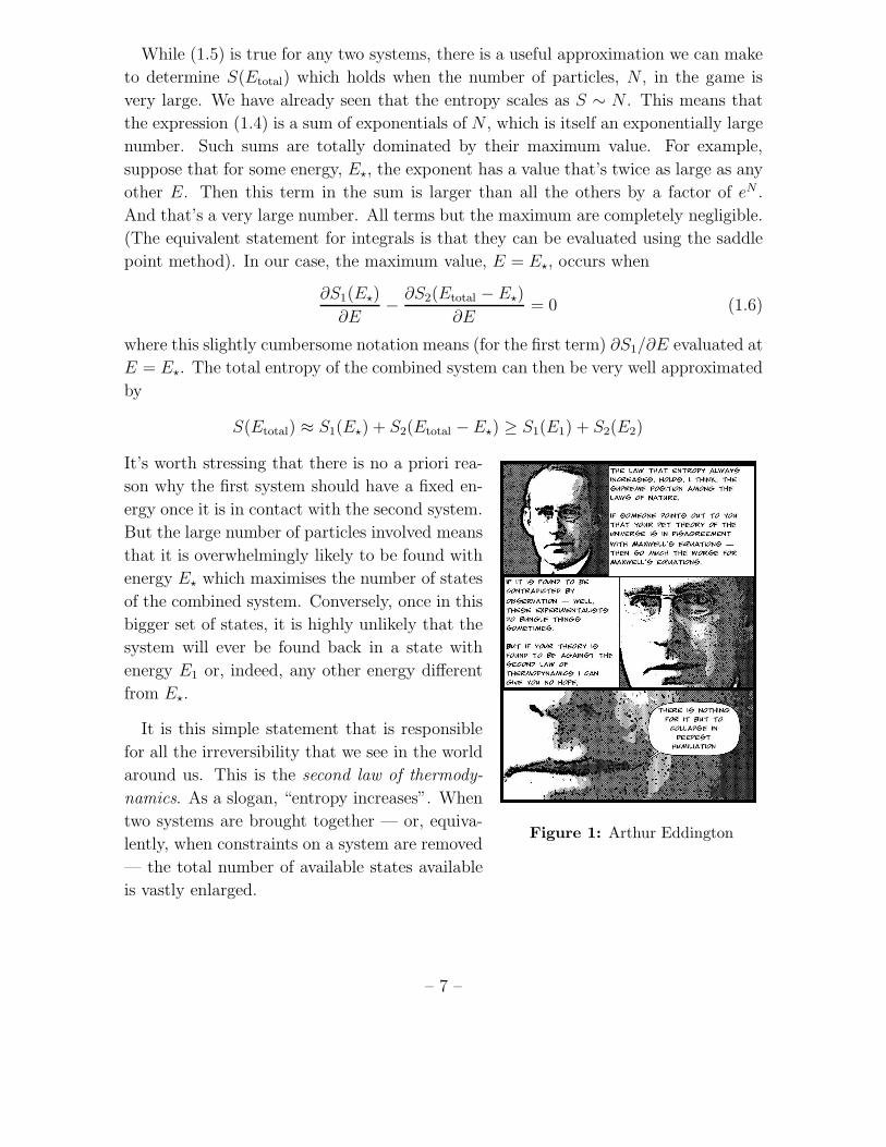
It’s worth stressing that there is no a priori rea-

Figure 1: Arthur Eddington

son why the first system should have a fixed en-

ergy once it is in contact with the second system.

But the large number of particles involved means

that it is overwhelmingly likely to be found with

energy E⋆ which maximises the number of states

of the combined system. Conversely, once in this

bigger set of states, it is highly unlikely that the

system will ever be found back in a state with

energy E1 or, indeed, any other energy different

from E⋆.

It is this simple statement that is responsible

for all the irreversibility that we see in the world

around us. This is the second law of thermody-

namics. As a slogan, “entropy increases”. When

two systems are brought together — or, equiva-

lently, when constraints on a system are removed

— the total number of available states available

is vastly enlarged.

– 7 –

It is sometimes stated that second law is the most sacred in all of physics. Arthur

Eddington’s rant, depicted in the cartoon, is one of the more famous acclamations of

the law.

And yet, as we have seen above, the second law hinges on probabilistic arguments.

We said, for example, that it is “highly unlikely” that the system will return to its

initial configuration. One might think that this may allow us a little leeway. Perhaps,

if probabilities are underlying the second law, we can sometimes get lucky and find

counterexamples. While, it is most likely to find system 1 to have energy E⋆, surely

occasionally one sees it in a state with a different energy? In fact, this never happens.

The phrase “highly unlikely” is used only because the English language does not contain

enough superlatives to stress how ridiculously improbable a violation of the second law

would be. The silly number of possible states in a macroscopic systems means that

violations happen only on silly time scales: exponentials of exponentials. This is a good

operational definition of the word “never”.

1.2.2 Temperature

We next turn to a very familiar quantity, albeit viewed in an unfamiliar way. The

temperature, T , of a system is defined as

1

T=∂S

∂E(1.7)

This is an extraordinary equation. We have introduced it as the definition of tempera-

ture. But why is this a good definition? Why does it agree with the idea of temperature

that your mum has? Why is this the same T that makes mercury rise (the element, not

the planet...that’s a different course). Why is it the same T that makes us yell when

we place our hand on a hot stove?

First, note that T has the right units, courtesy of Boltzmann’s constant (1.3). But

that was our merely a choice of convention: it doesn’t explain why T has the properties

that we expect of temperature. To make progress, we need to think more carefully

about the kind of properties that we do expect. We will describe this in some detail in

Section 4. For now it will suffice to describe the key property of temperature, which

is the following: suppose we take two systems, each in equilibrium and each at the

same temperature T , and place them in contact so that they can exchange energy.

Then...nothing happens.

It is simple to see that this follows from our definition (1.7). We have already done

the hard work above where we saw that two systems, brought into contact in this way,

– 8 –

will maximize their entropy. This is achieved when the first system has energy E⋆ and

the second energy Etotal−E⋆, with E⋆ determined by equation (1.6). If we want nothing

noticeable to happen when the systems are brought together, then it must have been

the case that the energy of the first system was already at E1 = E⋆. Or, in other words,

that equation (1.6) was obeyed before the systems were brought together,

∂S1(E1)

∂E=∂S2(E2)

∂E(1.8)

From our definition (1.7), this is the same as requiring that the initial temperatures of

the two systems are equal: T1 = T2.

Suppose now that we bring together two systems at slightly different temperatures.

They will exchange energy, but conservation ensures that what the first system gives

up, the second system receives and vice versa. So δE1 = −δE2. If the change of entropy

is small, it is well approximated by

δS =∂S1(E1)

∂EδE1 +

∂S2(E2)

∂EδE2

=

(

∂S1(E1)

∂E− ∂S2(E2)

∂E

)

δE1

=

(

1

T1− 1

T2

)

δE1

The second law tells us that entropy must increase: δS > 0. This means that if T1 > T2,

we must have δE1 < 0. In other words, the energy flows in the way we would expect:

from the hotter system to colder.

To summarise: the equilibrium argument tell us that ∂S/∂E should have the inter-

pretation as some function of temperature; the heat flowing argument tell us that it

should be a monotonically decreasing function. But why 1/T and not, say, 1/T 2? To

see this, we really need to compute T for a system that we’re all familiar with and see

that it gives the right answer. Once we’ve got the right answer for one system, the

equilibrium argument will ensure that it is right for all systems. Our first business in

Section 2 will be to compute the temperature T for an ideal gas and confirm that (1.7)

is indeed the correct definition.

Heat Capacity

The heat capacity, C, is defined by

C =∂E

∂T(1.9)

– 9 –

We will later introduce more refined versions of the heat capacity (in which various,

yet-to-be-specified, external parameters are held constant or allowed to vary and we are

more careful about the mode of energy transfer into the system). The importance of

the heat capacity is that it is defined in terms of things that we can actually measure!

Although the key theoretical concept is entropy, if you’re handed an experimental

system involving 1023 particles, you can’t measure the entropy directly by counting the

number of accessible microstates. You’d be there all day. But you can measure the

heat capacity: you add a known quantity of energy to the system and measure the rise

in temperature. The result is C−1.

There is another expression for the heat capacity that is useful. The entropy is a

function of energy, S = S(E). But we could invert the formula (1.7) to think of energy

as a function of temperature, E = E(T ). We then have the expression

∂S

∂T=∂S

∂E· ∂E∂T

=C

T

This is a handy formula. If we can measure the heat capactiy of the system for various

temperatures, we can get a handle on the function C(T ). From this we can then

determine the entropy of the system. Or, more precisely, the entropy difference

∆S =

∫ T2

T1

C(T )

TdT (1.10)

Thus the heat capacity is our closest link between experiment and theory.

The heat capacity is always proportional to N , the number of particles in the system.

It is common to define the specific heat capacity, which is simply the heat capacity

divided by the mass of the system and is independent of N .

There is one last point to make about heat capacity. Differentiating (1.7) once more,

we have

∂2S

∂E2= − 1

T 2C(1.11)

Nearly all systems you will meet have C > 0. (There is one important exception:

a black hole has negative heat capacity!). Whenever C > 0, the system is said to

be thermodynamically stable. The reason for this language goes back to the previous

discussion concerning two systems which can exchange energy. There we wanted to

maximize the entropy and checked that we had a stationary point (1.6), but we forgot

to check whether this was a maximum or minimum. It is guaranteed to be a maximum

if the heat capacity of both systems is positive so that ∂2S/∂E2 < 0.

– 10 –

1.2.3 An Example: The Two State System

Consider a system of N non-interacting particles. Each particle is fixed in position and

can sit in one of two possible states which, for convenience, we will call “spin up” | ↑ 〉and “spin down” |↓ 〉. We take the energy of these states to be,

E↓ = 0 , E↑ = ǫ

which means that the spins want to be down; you pay an energy cost of ǫ for each

spin which points up. If the system has N↑ particles with spin up and N↓ = N − N↑

particles with spin down, the energy of the system is

E = N↑ǫ

We can now easily count the number of states Ω(E) of the total system which have

energy E. It is simply the number of ways to pick N↑ particles from a total of N ,

Ω(E) =N !

N↑!(N −N↑)!

and the entropy is given by

S(E) = kB log

(

N !

N↑!(N −N↑)!

)

An Aside: Stirling’s Formula

For large N , there is a remarkably accurate approximation to the factorials that appear

in the expression for the entropy. It is known as Stirling’s formula,

logN ! = N logN −N + 12log 2πN + O(1/N)

You will prove this on the first problem sheet. How- log(p)

1 32 4 N

p

Figure 2:

ever, for our purposes we will only need the first two

terms in this expansion and these can be very quickly

derived by looking at the expression

logN ! =

N∑

p=1

log p ≈∫ N

1

dp log p = N logN −N + 1

where we have approximated the sum by the integral

as shown in the figure. You can also see from the

figure that integral gives a lower bound on the sum

which is confirmed by checking the next terms in Stirling’s formula.

– 11 –

Back to the Physics

Using Stirling’s approximation, we can write the entropy as

S(E) = kB [N logN −N −N↑ logN↑ +N↑ − (N −N↑) log(N −N↑) + (N −N↑)]

= −kB

[

(N −N↑) log

(

N −N↑

N

)

+N↑ log

(

N↑

N

)]

= −kBN

[(

1 − E

Nǫ

)

log

(

1 − E

Nǫ

)

+E

Nǫlog

(

E

Nǫ

)]

(1.12)

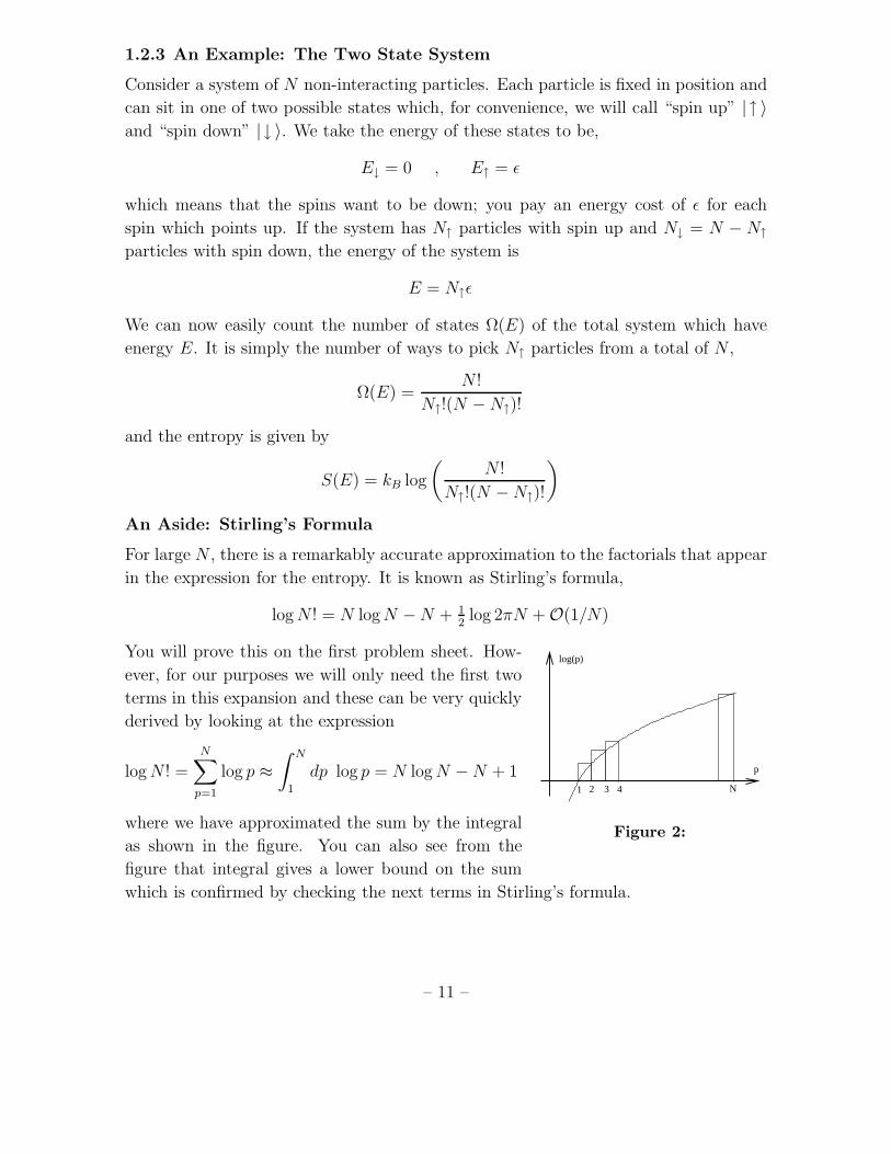
A sketch of S(E) plotted against E is shown in Figure 3. The entropy vanishes when

E = 0 (all spins down) and E = Nǫ (all spins up) because there is only one possible

state with each of these energies. The entropy is maximal when E = Nǫ/2 where we

have S = NkB log 2.

If the system has energy E, its temperature is

1

T=∂S

∂E=kB

ǫlog

(

Nǫ

E− 1

)

We can also invert this expression. If the system has temperature T , the fraction of

particles with spin up is given by

N↑

N=

E

Nǫ=

1

eǫ/kBT + 1(1.13)

Note that as T → ∞, the fraction of spins N↑/N → 1/2.

NεNε

S(E)

E

/2

Figure 3: Entropy of the

two-state system

In the limit of infinite temperature, the system sits at

the peak of the curve in Figure 3.

What happens for energies E > Nǫ/2, where N↑/N >

1/2? From the definition of temperature as 1/T = ∂S/∂E,

it is clear that we have entered the realm of negative

temperatures. This should be thought of as hotter than

infinity! (This is simple to see in the variables 1/T which

tends towards zero and then just keeps going to negative

values). Systems with negative temperatures have the

property that the number of microstates decreases as we

add energy. They can be realised in laboratories, at least temporarily, by instanta-

neously flipping all the spins in a system.

– 12 –

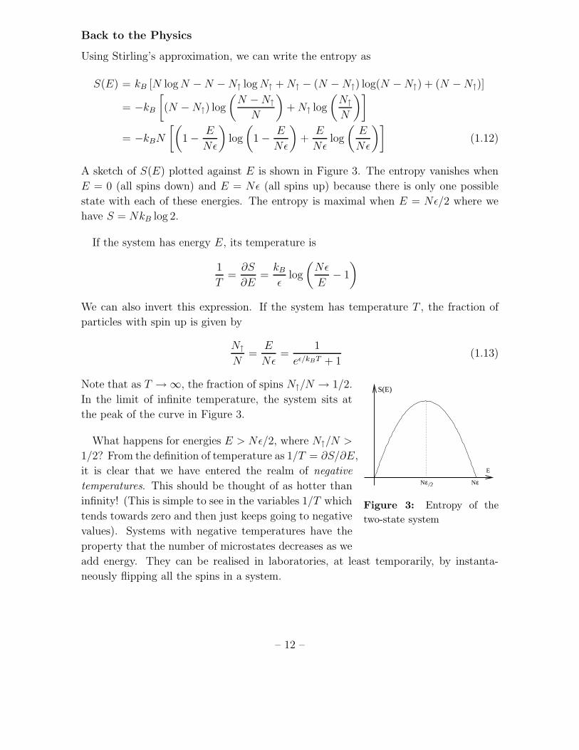
Heat Capacity and the Schottky Anomaly

Finally, we can compute the heat capacity, which we choose to express as a function

of temperature (rather than energy) since this is more natural when comparing to

experiment. We then have

C =dE

dT=

Nǫ2

kBT 2

eǫ/kBT

(eǫ/kBT + 1)2(1.14)

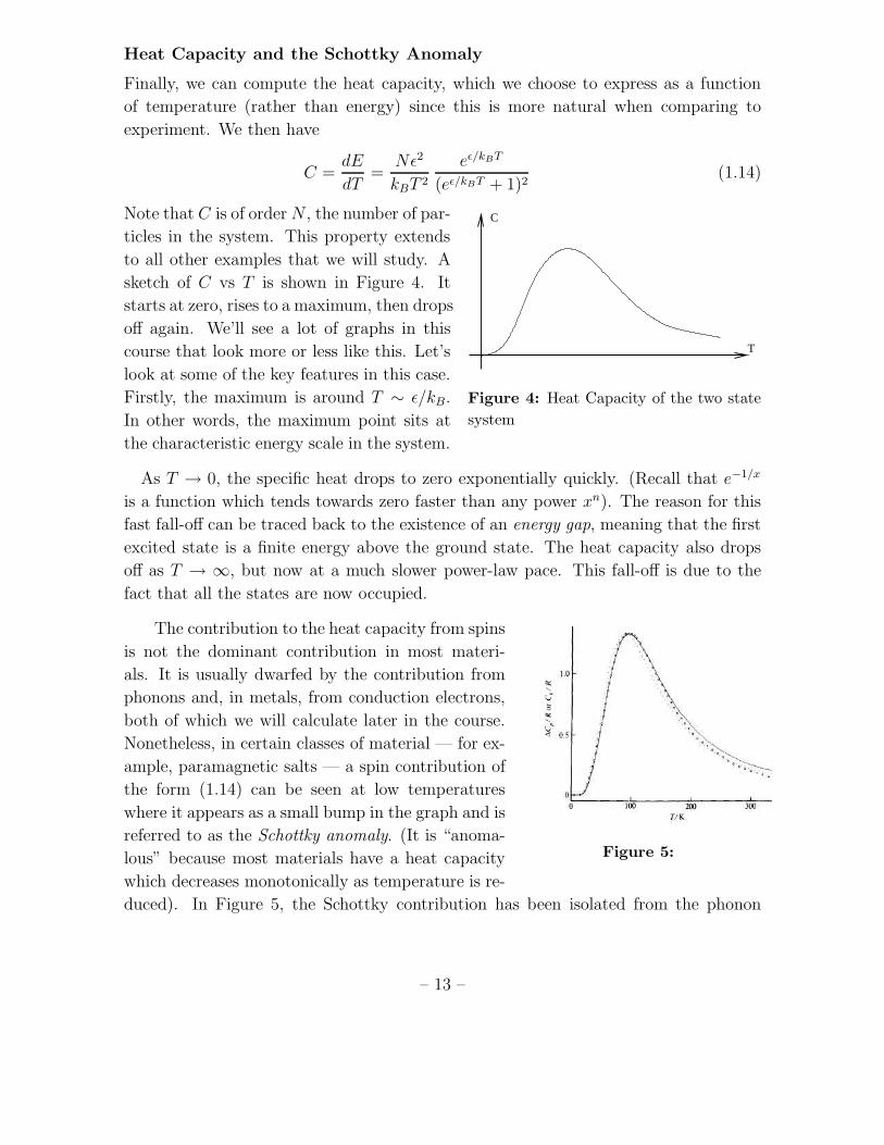
Note that C is of orderN , the number of par- C

T

Figure 4: Heat Capacity of the two state

system

ticles in the system. This property extends

to all other examples that we will study. A

sketch of C vs T is shown in Figure 4. It

starts at zero, rises to a maximum, then drops

off again. We’ll see a lot of graphs in this

course that look more or less like this. Let’s

look at some of the key features in this case.

Firstly, the maximum is around T ∼ ǫ/kB.

In other words, the maximum point sits at

the characteristic energy scale in the system.

As T → 0, the specific heat drops to zero exponentially quickly. (Recall that e−1/x

is a function which tends towards zero faster than any power xn). The reason for this

fast fall-off can be traced back to the existence of an energy gap, meaning that the first

excited state is a finite energy above the ground state. The heat capacity also drops

off as T → ∞, but now at a much slower power-law pace. This fall-off is due to the

fact that all the states are now occupied.

The contribution to the heat capacity from spins

Figure 5:

is not the dominant contribution in most materi-

als. It is usually dwarfed by the contribution from

phonons and, in metals, from conduction electrons,

both of which we will calculate later in the course.

Nonetheless, in certain classes of material — for ex-

ample, paramagnetic salts — a spin contribution of

the form (1.14) can be seen at low temperatures

where it appears as a small bump in the graph and is

referred to as the Schottky anomaly. (It is “anoma-

lous” because most materials have a heat capacity

which decreases monotonically as temperature is re-

duced). In Figure 5, the Schottky contribution has been isolated from the phonon

– 13 –

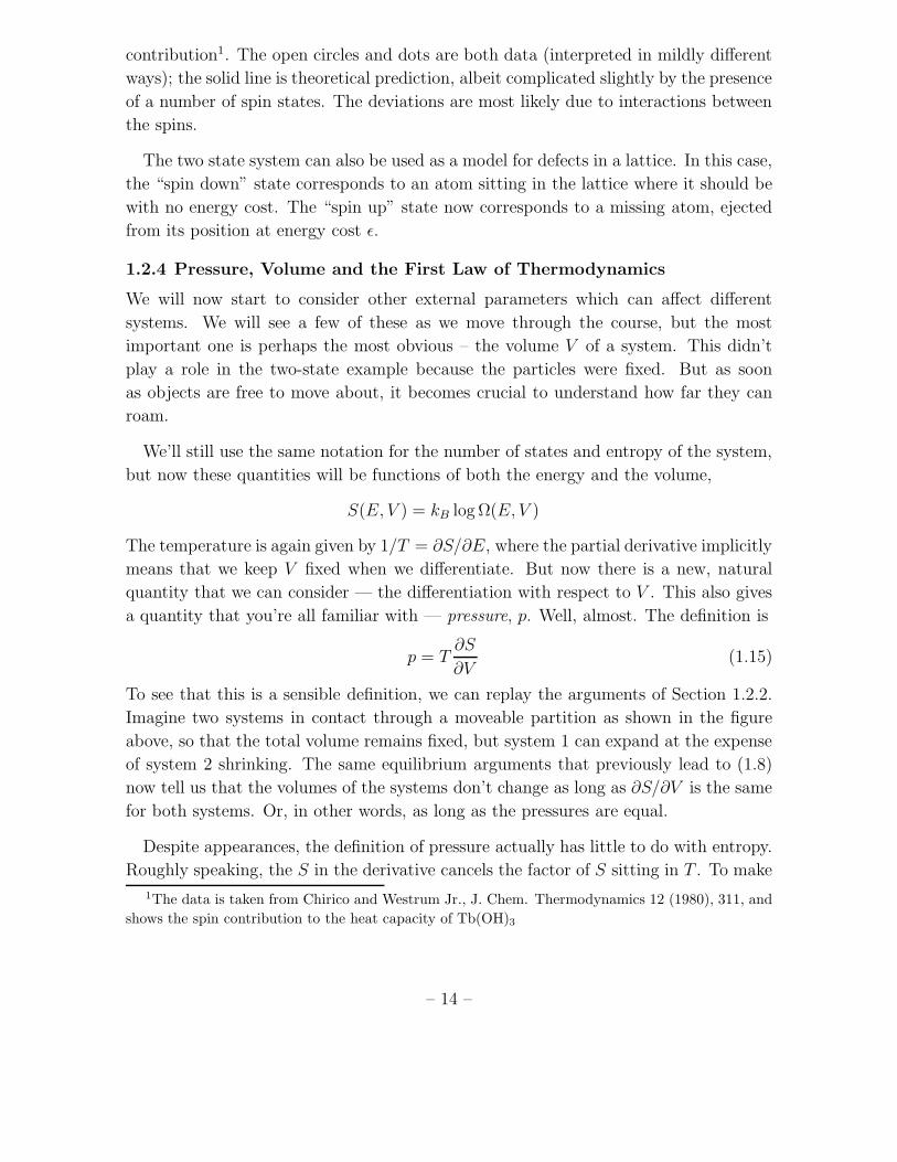
contribution1. The open circles and dots are both data (interpreted in mildly different

ways); the solid line is theoretical prediction, albeit complicated slightly by the presence

of a number of spin states. The deviations are most likely due to interactions between

the spins.

The two state system can also be used as a model for defects in a lattice. In this case,

the “spin down” state corresponds to an atom sitting in the lattice where it should be

with no energy cost. The “spin up” state now corresponds to a missing atom, ejected

from its position at energy cost ǫ.

1.2.4 Pressure, Volume and the First Law of Thermodynamics

We will now start to consider other external parameters which can affect different

systems. We will see a few of these as we move through the course, but the most

important one is perhaps the most obvious – the volume V of a system. This didn’t

play a role in the two-state example because the particles were fixed. But as soon

as objects are free to move about, it becomes crucial to understand how far they can

roam.

We’ll still use the same notation for the number of states and entropy of the system,

but now these quantities will be functions of both the energy and the volume,

S(E, V ) = kB log Ω(E, V )

The temperature is again given by 1/T = ∂S/∂E, where the partial derivative implicitly

means that we keep V fixed when we differentiate. But now there is a new, natural

quantity that we can consider — the differentiation with respect to V . This also gives

a quantity that you’re all familiar with — pressure, p. Well, almost. The definition is

p = T∂S

∂V(1.15)

To see that this is a sensible definition, we can replay the arguments of Section 1.2.2.

Imagine two systems in contact through a moveable partition as shown in the figure

above, so that the total volume remains fixed, but system 1 can expand at the expense

of system 2 shrinking. The same equilibrium arguments that previously lead to (1.8)

now tell us that the volumes of the systems don’t change as long as ∂S/∂V is the same

for both systems. Or, in other words, as long as the pressures are equal.

Despite appearances, the definition of pressure actually has little to do with entropy.

Roughly speaking, the S in the derivative cancels the factor of S sitting in T . To make

1The data is taken from Chirico and Westrum Jr., J. Chem. Thermodynamics 12 (1980), 311, and

shows the spin contribution to the heat capacity of Tb(OH)3

– 14 –

this mathematically precise, consider a system with entropy S(E, V ) that undergoes a

small change in energy and volume. The change in entropy is

dS =∂S

∂EdE +

∂S

∂VdV

Rearranging, and using our definitions (1.7) and (1.15), we can write

dE = TdS − pdV (1.16)

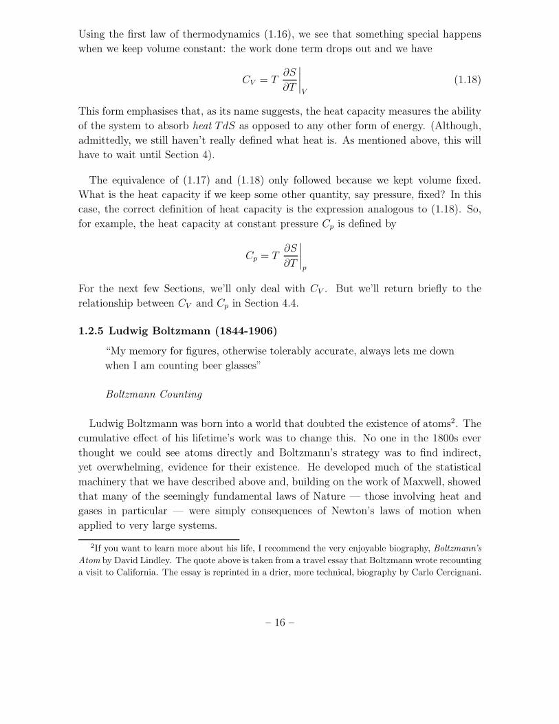
The left-hand side is the change in energy of the system.

Pressure, pdx

Area, A

Figure 7: Work Done

It is easy to interpret the second term on the right-hand

side: it is the work done on the system. To see this,

consider the diagram on the right. Recall that pressure

is force per area. The change of volume in the set-up

depicted is dV = Area × dx. So the work done on the

system is Force × dx = (pA)dx = pdV . To make sure

that we’ve got the minus signs right, remember that if

dV < 0, we’re exerting a force to squeeze the system, increasing its energy. In contrast,

if dV > 0, the system itself is doing the work and hence losing energy.

Alternatively, you may prefer to run this argument in reverse: if you’re happy to

equate squeezing the system by dV with doing work, then the discussion above is

sufficient to tell you that pressure as defined in (1.15) has the interpretation of force

per area.

What is the interpretation of the first term on the right-hand side of (1.16)? It

must be some form of energy transferred to the system. It turns out that the correct

interpretation of TdS is the amount of heat the system absorbs from the surroundings.

Much of Section 4 will be concerned with understanding why this is right way to think

about TdS and we postpone a full discussion until then.

Equation (1.16) expresses the conservation of energy for a system at finite temper-

ature. It is known as the First Law of Thermodynamics. (You may have noticed that

we’re not doing these laws in order! This too will be rectified in Section 4).

As a final comment, we can now give a slightly more refined definition of the heat

capacity (1.9). In fact, there are several different heat capacities which depend on

which other variables are kept fixed. Throughout most of these lectures, we will be

interested in the heat capacity at fixed volume, denoted CV ,

CV =∂E

∂T

∣

∣

∣

∣

V

(1.17)

– 15 –

Using the first law of thermodynamics (1.16), we see that something special happens

when we keep volume constant: the work done term drops out and we have

CV = T∂S

∂T

∣

∣

∣

∣

V

(1.18)

This form emphasises that, as its name suggests, the heat capacity measures the ability

of the system to absorb heat TdS as opposed to any other form of energy. (Although,

admittedly, we still haven’t really defined what heat is. As mentioned above, this will

have to wait until Section 4).

The equivalence of (1.17) and (1.18) only followed because we kept volume fixed.

What is the heat capacity if we keep some other quantity, say pressure, fixed? In this

case, the correct definition of heat capacity is the expression analogous to (1.18). So,

for example, the heat capacity at constant pressure Cp is defined by

Cp = T∂S

∂T

∣

∣

∣

∣

p

For the next few Sections, we’ll only deal with CV . But we’ll return briefly to the

relationship between CV and Cp in Section 4.4.

1.2.5 Ludwig Boltzmann (1844-1906)

“My memory for figures, otherwise tolerably accurate, always lets me down

when I am counting beer glasses”

Boltzmann Counting

Ludwig Boltzmann was born into a world that doubted the existence of atoms2. The

cumulative effect of his lifetime’s work was to change this. No one in the 1800s ever

thought we could see atoms directly and Boltzmann’s strategy was to find indirect,

yet overwhelming, evidence for their existence. He developed much of the statistical

machinery that we have described above and, building on the work of Maxwell, showed

that many of the seemingly fundamental laws of Nature — those involving heat and

gases in particular — were simply consequences of Newton’s laws of motion when

applied to very large systems.

2If you want to learn more about his life, I recommend the very enjoyable biography, Boltzmann’s

Atom by David Lindley. The quote above is taken from a travel essay that Boltzmann wrote recounting

a visit to California. The essay is reprinted in a drier, more technical, biography by Carlo Cercignani.

– 16 –

It is often said that Boltzmann’s great insight was the equation which is now engraved

on his tombstone, S = kB log Ω, which lead to the understanding of the second law of

thermodynamics in terms of microscopic disorder. Yet these days it is difficult to

appreciate the boldness of this proposal simply because we rarely think of any other

definition of entropy. We will, in fact, meet the older thermodynamic notion of entropy

and the second law in Section 4 of this course. In the meantime, perhaps Boltzmann’s

genius is better reflected in the surprising equation for temperature: 1/T = ∂S/∂E.

Boltzmann gained prominence during his lifetime, holding professorships at Graz,

Vienna, Munich and Leipzig (not to mention a position in Berlin that he somehow

failed to turn up for). Nonetheless, his work faced much criticism from those who

would deny the existence of atoms, most notably Mach. It is not known whether these

battles contributed to the depression Boltzmann suffered later in life, but the true

significance of his work was only appreciated after his body was found hanging from

the rafters of a guest house near Trieste.

1.3 The Canonical Ensemble

The microcanonical ensemble describes systems that have a fixed energy E. From this,

we deduce the equilibrium temperature T . However, very often this is not the best way

to think about a system. For example, a glass of water sitting on a table has a well

defined average energy. But the energy is constantly fluctuating as it interacts with

the environment. For such systems, it is often more appropriate to think of them as

sitting at fixed temperature T , from which we then deduce the average energy.

To model this, we will consider a system — let’s call it S — in contact with a second

system which is a large heat reservoir – let’s call it R. This reservoir is taken to be

at some equilibrium temperature T . The term “reservoir” means that the energy of S

is negligible compared with that of R. In particular, S can happily absorb or donate

energy from or to the reservoir without changing the ambient temperature T .

How are the energy levels of S populated in such a situation? We label the states

of S as |n〉, each of which has energy En. The number of microstates of the combined

systems S and R is given by the sum over all states of S,

Ω(Etotal) =∑

n

ΩR(Etotal − En) ≡∑

n

exp

(

SR(Etotal − En)

kB

)

I stress again that the sum above is over all the states of S, rather than over the energy

levels of S. (If we’d written the latter, we would have to include a factor of ΩS(En) in

the sum to take into account the degeneracy of states with energy En). The fact that

– 17 –

R is a reservoir means that En ≪ Etotal. This allows us to Taylor expand the entropy,

keeping just the first two terms,

Ω(Etotal) ≈∑

n

exp

(

SR(Etotal)

kB− ∂SR

∂Etotal

En

kB

)

But we know that ∂SR/∂Etotal = 1/T , so we have

Ω(Etotal) = eSR(Etotal)/kB

∑

n

e−En/kBT

We now apply the fundamental assumption of statistical mechanics — that all accessible

energy states are equally likely — to the combined system + reservoir. This means

that each of the Ω(Etotal) states above is equally likely. The number of these states for

which the system sits in |n〉 is eSR/kBe−En/kBT . So the probabilty that the system sits

in state |n〉 is just the ratio of this number of states to the total number of states,

p(n) =e−En/kBT

∑

m e−Em/kBT

(1.19)

This is the Boltzmann distribution, also known as the canonical ensemble. Notice that

the details of the reservoir have dropped out. We don’t need to know SR(E) for the

reservoir; all that remains of its influence is the temperature T .

The exponential suppression in the Boltzmann distribution means that it is very

unlikely that any of the states with En ≫ kBT are populated. However, all states

with energy En ≤ kBT have a decent chance of being occupied. Note that as T → 0,

the Boltzmann distribution forces the system into its ground state (i.e. the state with

lowest energy); all higher energy states have vanishing probability at zero temperature.

1.3.1 The Partition Function

Since we will be using various quantities a lot, it is standard practice to introduce new

notation. Firstly, the inverse factor of the temperature is universally denoted,

β ≡ 1

kBT(1.20)

And the normalization factor that sits in the denominator of the probability is written,

Z =∑

n

e−βEn (1.21)

In this notation, the probability for the system to be found in state |n〉 is

p(n) =e−βEn

Z(1.22)

– 18 –

Rather remarkably, it turns out that the most important quantity in statistical me-

chanics is Z. Although this was introduced as a fairly innocuous normalization factor,

it actually contains all the information we need about the system. We should think of

Z, as defined in (1.21), as a function of the (inverse) temperature β. When viewed in

this way, Z is called the partition function.

We’ll see lots of properties of Z soon. But we’ll start with a fairly basic, yet impor-

tant, point: for independent systems, Z’s multiply. This is easy to prove. Suppose that

we have two systems which don’t interact with each other. The energy of the combined

system is then just the sum of the individual energies. The partition function for the

combined system is (in, hopefully, obvious notation)

Z =∑

n,m

e−β(E(1)n +E

(2)m )

=∑

n,m

e−βE(1)n e−βE

(2)m

=∑

n

e−βE(1)n

∑

m

e−βE(2)m = Z1Z2 (1.23)

A Density Matrix for the Canonical Ensemble

In statistical mechanics, the inherent probabilities of the quantum world are joined

with probabilities that arise from our ignorance of the underlying state. The correct

way to describe this is in term of a density matrix, ρ. The canonical ensemble is really

a choice of density matrix,

ρ =e−βH

Z(1.24)

If we make a measurement described by an operator O, then the probability that we

find ourselves in the eigenstate |φ〉 is given by

p(φ) = 〈φ|ρ|φ〉

For energy eigenstates, this coincides with our earlier result (1.22). We won’t use the

language of density matrices in this course, but it is an elegant and conceptually clear

framework to describe more formal results.

1.3.2 Energy and Fluctuations

Let’s see what information is contained in the partition function. We’ll start by think-

ing about the energy. In the microcanonical ensemble, the energy was fixed. In the

– 19 –

canonical ensemble, that is no longer true. However, we can happily compute the

average energy,

〈E〉 =∑

n

p(n)En =∑

n

Ene−βEn

Z

But this can be very nicely expressed in terms of the partition function by

〈E〉 = − ∂

∂βlogZ (1.25)

We can also look at the spread of energies about the mean — in other words, about

fluctuations in the probability distribution. As usual, this spread is captured by the

variance,

∆E2 = 〈(E − 〈E〉)2〉 = 〈E2〉 − 〈E〉2

This too can be written neatly in terms of the partition function,

∆E2 =∂2

∂β2logZ = −∂〈E〉

∂β(1.26)

There is another expression for the fluctuations that provides some insight. Recall our

definition of the heat capacity (1.9) in the microcanonical ensemble. In the canonical

ensemble, where the energy is not fixed, the corresponding definition is

CV =∂〈E〉∂T

∣

∣

∣

∣

V

Then, since β = 1/kBT , the spread of energies in (1.26) can be expressed in terms of

the heat capacity as

∆E2 = kBT2CV (1.27)

There are two important points hiding inside this small equation. The first is that the

equation relates two rather different quantities. On the left-hand side, ∆E describes

the probabilistic fluctuations in the energy of the system. On the right-hand side, the

heat capacity CV describes the ability of the system to absorb energy. If CV is large,

the system can take in a lot of energy without raising its temperature too much. The

equation (1.27) tells us that the fluctuations of the systems are related to the ability of

the system to dissipate, or absorb, energy. This is the first example of a more general

result known as the fluctuation-dissipation theorem.

– 20 –

The other point to take away from (1.27) is the size of the fluctuations as the number

of particles N in the system increases. Typically E ∼ N and CV ∼ N . Which means

that the relative size of the fluctuations scales as

∆E

E∼ 1√

N(1.28)

The limit N → ∞ in known as the thermodynamic limit. The energy becomes peaked

closer and closer to the mean value 〈E〉 and can be treated as essentially fixed. But

this was our starting point for the microcanonical ensemble. In the thermodynamic

limit, the microcanonical and canonical ensembles coincide.

All the examples that we will discuss in the course will have a very large number of

particles, N , and we can consider ourselves safely in the thermodynamic limit. For that

reason, even in the canonical ensemble, we will often write E for the average energy

rather than 〈E〉.

An Example: The Two State System Revisited

We can rederive our previous results for the two state system using the canonical

ensemble. It is marginally simpler. For a single particle with two energy levels, 0 and

ǫ, the partition function is given by

Z1 =∑

n

e−βEn = 1 + e−βǫ = 2e−βǫ/2 cosh(βǫ/2)

We want the partition function for N such particles. But we saw in (1.23) that if we

have independent systems, then we simply need to multiply their partition functions

together. We then have

Z = 2Ne−Nβǫ/2 coshN (βǫ/2)

from which we can easily compute the average energy

〈E〉 = − ∂

∂βlogZ =

Nǫ

2(1 − tanh(βǫ/2))

A bit of algebra will reveal that this is the same expression that we derived in the

microcanonical ensemble (1.13). We could now go on to compute the heat capacity

and reproduce the result (1.14).

Notice that, unlike in the microcanonical ensemble, we didn’t have to solve any

combinatoric problem to count states. The partition function has done all that work

for us. Of course, for this simple two state system, the counting of states wasn’t difficult

but in later examples, where the counting gets somewhat tricker, the partition function

will be an invaluable tool to save us the work.

– 21 –

1.3.3 Entropy

Recall that in the microcanonical ensemble, the entropy counts the (log of the) number

of states with fixed energy. We would like to define an analogous quantity in the

canonical ensemble where we have a probability distribution over states with different

energies. How to proceed? Our strategy will be to again return to the microcanonical

ensemble, now applied to the combined system + reservoir.

In fact, we’re going to use a little trick. Suppose that we don’t have just one copy

of our system S, but instead a large number, W , of identical copies. Each system lives

in a particular state |n〉. If W is large enough, the number of systems that sit in state

|n〉 must be simply p(n)W . We see that the trick of taking W copies has translated

the probabilities into eventualities. To determine the entropy we can treat the whole

collection of W systems as sitting in the microcanonical ensemble to which we can

apply the familiar Boltzmann definition of entropy (1.2). We must only figure out how

many ways there are of putting p(n)W systems into state |n〉 for each |n〉. That’s a

simple combinatoric problem: the answer is

Ω =W !

∏

n(p(n)W )!

And the entropy is therefore

S = kB log Ω = −kBW∑

n

p(n) log p(n) (1.29)

where we have used Stirling’s formula to simplify the logarithms of factorials. This is

the entropy for all W copies of the system. But we also know that entropy is additive.

So the entropy for a single copy of the system, with probability distribution p(n) over

the states is

S = −kB

∑

n

p(n) log p(n) (1.30)

This beautiful formula is due to Gibbs. It was rediscovered some decades later in the

context of information theory where it goes by the name of Shannon entropy for classical

systems or von Neumann entropy for quantum systems. In the quantum context, it is

sometimes written in terms of the density matrix (1.24) as

S = −kBTr ρ log ρ

When we first introduced entropy in the microcanonical ensemble, we viewed it as a

function of the energy E. But (1.30) gives a very different viewpoint on the entropy:

– 22 –

it says that we should view S as a function of a probability distribution. There is

no contradiction with the microcanonical ensemble because in that simple case, the

probability distribution is itself determined by the choice of energy E. Indeed, it

is simple to check (and you should!) that the Gibbs entropy (1.30) reverts to the

Boltzmann entropy in the special case of p(n) = 1/Ω(E) for all states |n〉 of energy E.

Meanwhile, back in the canonical ensemble, the probability distribution is entirely

determined by the choice of temperature T . This means that the entropy is naturally

a function of T . Indeed, substituting the Boltzmann distribution p(n) = e−βEn/Z into

the expression (1.30), we find that the entropy in the canonical ensemble is given by

S = −kB

Z

∑

n

e−βEn log

(

e−βEn

Z

)

=kBβ

Z

∑

n

Ene−βEn + kB logZ

As with all other important quantities, this can be elegantly expressed in terms of the

partition function by

S = kB∂

∂T(T logZ) (1.31)

A Comment on the Microcanonical vs Canonical Ensembles

The microcanonical and canonical ensembles are different probability distributions.

This means, using the definition (1.30), that they generally have different entropies.

Nonetheless, in the limit of a large number of particles, N → ∞, all physical observables

— including entropy — coincide in these two distributions. We’ve already seen this

when we computed the variance of energy (1.28) in the canonical ensemble. Let’s take

a closer look at how this works.

The partition function in (1.21) is a sum over all states. We can rewrite it as a sum

over energy levels by including a degeneracy factor

Z =∑

Ei

Ω(Ei)e−βEi

The degeneracy factor Ω(E) factor is typically a rapidly rising function of E, while the

Boltzmann suppression e−βE is rapidly falling. But, for both the exponent is propor-

tional to N which is itself exponentially large. This ensures that the sum over energy

levels is entirely dominated by the maximum value, E⋆, defined by the requirement

∂

∂E

(

Ω(E)e−βE)

E=E⋆

= 0

– 23 –

and the partition function can be well approximated by

Z ≈ Ω(E⋆)e−βE⋆

(This is the same kind of argument we used in (1.2.1) in our discussion of the Second

Law). With this approximation, we can use (1.25) to show that the most likely energy

E⋆ and the average energy 〈E〉 coincide:

〈E〉 = E⋆

(We need to use the result (1.7) in the form ∂ log Ω(E⋆)/∂E⋆ = β to derive this).

Similarly, using (1.31), we can show that the entropy in the canonical ensemble is given

by

S = kB log Ω(E⋆)

Maximizing Entropy

There is actually a unified way to think about the microcanonical and canonical ensem-

bles in terms of a variational principle: the different ensembles have the property that

they maximise the entropy subject to various constraints. The only difference between

them is the constraints that are imposed.

Let’s start with the microcanonical ensemble, in which we fix the energy of the system

so that we only allow non-zero probabilities for those states which have energy E. We

could then compute the entropy using the Gibbs formula (1.30) for any probability

distribution, including systems away from equilibrium. We need only insist that all the

probabilities add up to one:∑

n p(n) = 1. We can maximise S subject to this condition

by introducing a Lagrange multiplier α and maximising S + αkB(∑

n p(n) − 1),

∂

∂p(n)

(

−∑

n

p(n) log p(n) + α∑

n

p(n) − α

)

= 0 ⇒ p(n) = eα−1

We learn that all states with energy E are equally likely. This is the microcanonical

ensemble.

In the examples sheet, you will be asked to show that the canonical ensemble can be

viewed in the same way: it is the probability distribution that maximises the entropy

subject to the constraint that the average energy is fixed.

– 24 –

1.3.4 Free Energy

We’ve left the most important quantity in the canonical ensemble to last. It is called

the free energy,

F = 〈E〉 − TS (1.32)

There are actually a number of quantities all vying for the name “free energy”, but the

quantity F is the one that physicists usually work with. When necessary to clarify, it is

sometimes referred to as the Helmholtz free energy. The word “free” here doesn’t mean

“without cost”. Energy is never free in that sense. Rather, it should be interpreted as

the “available” energy.

Heuristically, the free energy captures the competition between energy and entropy

that occurs in a system at constant temperature. Immersed in a heat bath, energy

is not necessarily at a premium. Indeed, we saw in the two-state example that the

ground state plays little role in the physics at non-zero temperature. Instead, the role

of entropy becomes more important: the existence of many high energy states can beat

a few low-energy ones.

The fact that the free energy is the appropriate quantity to look at for systems at

fixed temperature is also captured by its mathematical properties. Recall, that we

started in the microcanonical ensemble by defining entropy S = S(E, V ). If we invert

this expression, then we can equally well think of energy as a function of entropy and

volume: E = E(S, V ). This is reflected in the first law of thermodynamics (1.16) which

reads dE = TdS − pdV . However, if we look at small variations in F , we get

dF = d〈E〉 − d(TS) = −SdT − pdV (1.33)

This form of the variation is telling us that we should think of the free energy as a

function of temperature and volume: F = F (T, V ). Mathematically, F is a Legendre

transform of E.

Given the free energy, the variation (1.33) tells us how to get back the entropy,

S = − ∂F

∂T

∣

∣

∣

∣

V

(1.34)

Similarly, the pressure is given by

p = − ∂F

∂V

∣

∣

∣

∣

T

(1.35)

– 25 –

The free energy is the most important quantity at fixed temperature. It is also the

quantity that is most directly related to the partition function Z:

F = −kBT logZ (1.36)

This relationship follows from (1.25) and (1.31). Using the identity ∂/∂β = −kBT2∂/∂T ,

these expressions allow us to write the free energy as

F = E − TS = kBT2 ∂

∂TlogZ − kBT

∂

∂T(T logZ)

= −kBT logZ

as promised.

1.4 The Chemical Potential

Before we move onto applications, there is one last bit of formalism that we will need to

introduce. This arises in situations where there is some other conserved quantity which

restricts the states that are accessible to the system. The most common example is

simply the number of particles N in the system. Another example is the electric charge

Q. For the sake of definiteness, we will talk about particle number below but all the

comments apply to any conserved quantity.

In both the microcanonical and canonical ensembles, we should only consider states

that have a fixed value of N . We already did this when we discussed the two state

system — for example, the expression for entropy (1.12) depends explicitly on the

number of particles N . We will now make this dependence explicit and write

S(E, V,N) = kB log Ω(E, V,N)

The entropy leads us to the temperature as 1/T = ∂S/∂E and the pressure as p =

T∂S/∂V . But now we have another option: we can differentiate with respect to particle

number N . The resulting quantity is called the chemical potential,

µ = −T ∂S∂N

(1.37)

Using this definition, we can re-run the arguments given in Section 1.2.2 for systems

which are allowed to exchange particles. Such systems are in equilibrium only if they

have equal chemical potential µ. This condition is usually referred to as chemical

equilibrium.

– 26 –

To get a feel for the meaning of the chemical potential, we can look again at the first

law of thermodynamics (1.16), now allowing for a change in particle number as well.

Writing dS = . . . and rearranging, we have,

dE = TdS − pdV + µdN (1.38)

This tells us the meaning of the chemical potential: it is the energy cost to add one

more particle to the system while keeping both S and V fixed. (Strictly speaking, an

infinitesimal amount of particle, but if we’re adding one more to 1023 that effectively

counts as infinitesimal). If we’re interested in electric charge Q, rather than particle

number, the chemical potential is the same thing as the familiar electrostatic potential

of the system that you met in your first course in electromagnetism.

There’s actually a subtle point in the above derivation that is worth making explicit.

It’s the kind of thing that will crop up a lot in thermodynamics where you typically

have many variables and need to be careful about which ones are kept fixed. We defined

the chemical potential as µ = −T ∂S/∂N |E,V . But the first law is telling us that we

can also think of the chemical potential as µ = ∂E/∂N |S,V . Why is this the same

thing? This follows from a general formula for partial derivatives. If you have three

variables, x, y and z, with a single constraint between them, then

∂x

∂y

∣

∣

∣

∣

z

∂y

∂z

∣

∣

∣

∣

x

∂z

∂x

∣

∣

∣

∣

y

= −1

Applying this general formula to E, S and N gives us the required result

∂E

∂N

∣

∣

∣

∣

S,V

= − ∂S

∂N

∣

∣

∣

∣

E,v

∂E

∂S

∣

∣

∣

∣

N,V

= µ

If we work at constant temperature rather than constant energy, the relevant function

is the free energy F (T, V,N) = E − TS. Small changes are given by

dF = −SdT − pdV + µdN

from which we see that the chemical potential can also be defined as

µ =∂F

∂N

∣

∣

∣

∣

T,V

1.4.1 Grand Canonical Ensemble

When we made the transition from microcanonical to canonical ensemble, we were no

longer so rigid in our insistence that the system has a fixed energy. Rather it could freely

– 27 –

exchange energy with the surrounding reservoir, which was kept at a fixed temperature.

We could now imagine the same scenario with any other conserved quantity. For

example, if particles are free to move between the system and the reservoir, then N

is no longer fixed. In such a situation, we will require that the reservoir sits at fixed

chemical potential µ as well as fixed temperature T .

The probability distribution that we need to use in this case is called the grand

canonical ensemble. The probability of finding the system in a state |n〉 depends on both

the energy En and the particle number Nn. (Notice that because N is conserved, the

quantum mechanical operator necessarily commutes with the Hamiltonian so there is

no difficulty in assigning both energy and particle number to each state). We introduce

the grand canonical partition function

Z(T, µ, V ) =∑

n

e−β(En−µNn) (1.39)

Re-running the argument that we used for the canonical ensemble, we find the proba-

bility that the system is in state |n〉 to be

p(n) =e−β(En−µNn)

ZIn the canonical ensemble, all the information that we need is contained within the

partition function Z. In the grand canonical ensemble it is contained within Z. The

entropy (1.30) is once again given by

S = kB∂

∂T(T logZ) (1.40)

while differentiating with respect to β gives us

〈E〉 − µ〈N〉 = − ∂

∂βlogZ (1.41)

The average particle number 〈N〉 in the system can then be separately extracted by

〈N〉 =1

β

∂

∂µlogZ (1.42)

and its fluctuations,

∆N2 =1

β2

∂2

∂µ2logZ =

1

β

∂〈N〉∂µ

(1.43)

Just as the average energy is determined by the temperature in the canonical ensemble,

here the average particle number is determined by the chemical potential. The grand

canonical ensemble will simplify several calculations later, especially when we come to

discuss Bose and Fermi gases in Section 3.

– 28 –

The relative size of these fluctuations scales in the same way as the energy fluctua-

tions, ∆N/〈N〉 ∼ 1/√

〈N〉, and in the thermodynamic limit N → ∞ results from all

three ensembles coincide. For this reason, we will drop the averaging brackets 〈·〉 from

our notation and simply refer to the average particle number as N .

1.4.2 Grand Canonical Potential

The grand canonical potential Φ is defined by

Φ = F − µN

Φ is a Legendre transform of F , from variable N to µ. This is underlined if we look at

small variations,

dΦ = −SdT − pdV −Ndµ (1.44)

which tells us that Φ should be thought of as a function of temperature, volume and

chemical potential, Φ = Φ(T, V, µ).

We can perform the same algebraic manipulations that gave us F in terms of the

canonical partition function Z, this time using the definitions (1.40) and (1.41)) to

write Φ as

Φ = −kBT logZ (1.45)

1.4.3 Extensive and Intensive Quantities

There is one property of Φ that is rather special and, at first glance, somewhat sur-

prising. This property actually follows from very simple considerations of how different

variables change as we look at bigger and bigger systems.

Suppose we have a system and we double it. That means that we double the volume

V , double the number of particles N and double the energy E. What happens to all our

other variables? We have already seen back in Section 1.2.1 that entropy is additive, so

S also doubles. More generally, if we scale V , N and E by some amount λ, the entropy

must scale as

S(λE, λV, λN) = λS(E, V,N)

Quantities such as E, V , N and S which scale in this manner are called extensive. In

contrast, the variables which arise from differentiating the entropy, such as temperature

1/T = ∂S/∂E and pressure p = T∂S/∂V and chemical potential µ = T∂S/∂N involve

the ratio of two extensive quantities and so do not change as we scale the system: they

are called intensive quantities.

– 29 –

What now happens as we make successive Legendre transforms? The free energy

F = E − TS is also extensive (since E and S are extensive while T is intensive). So it

must scale as

F (T, λV, λN) = λF (T, V,N) (1.46)

Similarly, the grand potential Φ = F − µN is extensive and scales as

Φ(T, λV, µ) = λΦ(T, V, µ) (1.47)

But there’s something special about this last equation, because Φ only depends on a

single extensive variable, namely V . While there are many ways to construct a free

energy F which obeys (1.46) (for example, any function of the form F ∼ V n+1/Nn will

do the job), there is only one way to satisfy (1.47): Φ must be proportional to V . But

we’ve already got a name for this proportionality constant: it is pressure. (Actually, it

is minus the pressure as you can see from (1.44)). So we have the equation

Φ(T, V, µ) = −p(T, µ)V (1.48)

It looks as if we got something for free! If F is a complicated function of V , where

do these complications go after the Legendre transform to Φ? The answer is that the

complications go into the pressure p(T, µ) when expressed as a function of T and µ.

Nonetheless, equation (1.48) will prove to be an extremely economic way to calculate

the pressure of various systems.

1.4.4 Josiah Willard Gibbs (1839-1903)

Gibbs was perhaps the first great American theoretical physicist. Many of the de-

velopments that we met in this chapter are due to him, including the free energy,

the chemical potential and, most importantly, the idea of ensembles. Even the name

“statistical mechanics” was invented by Gibbs.

Gibbs provided the first modern rendering of the subject in a treatise published

shortly before his death. Very few understood it. Lord Rayleigh wrote to Gibbs

suggesting that the book was “too condensed and too difficult for most, I might say

all, readers”. Gibbs disagreed. He wrote back saying the book was only “too long”.

There do not seem to be many exciting stories about Gibbs. He was an undergraduate

at Yale. He did a PhD at Yale. He became a professor at Yale. Apparently he rarely

left New Haven. Strangely, he did not receive a salary for the first ten years of his

professorship. Only when he received an offer from John Hopkins of $3000 dollars a

year did Yale think to pay America’s greatest physicist. They made a counter-offer of

$2000 dollars and Gibbs stayed.

– 30 –