Embed Size (px)
Citation preview
1
Statistical Physics an overview: up to Lect26a narrative version
Dec 3, 2012 version
Yoshi Oono [email protected] (3111 ESB, 2405 IGB)Physics and IGB, UIUC
This is a ‘reader’ accompanying Invitation to Statistical Physics, but actually acollection of transcripts of the actual lectures (augmented a bit sometimes). Thefluctuation-dissipation explanation is still complicated, and will be simplified.

2
Contents
1 Lecture 1: An introductory overview . . . . . . . . . . . . . . . . . . 52 Lecture 2: Atomic picture of gases + Introduction to Probability . . . 153 Lecture 3: Law of large numbers . . . . . . . . . . . . . . . . . . . . . 264 Lecture 4: Maxwell’s distribution . . . . . . . . . . . . . . . . . . . . 355 Lecture 5: Simple kinetic theory of transport phenomena . . . . . . . 436 Lecture 6: Brownian motion 2 . . . . . . . . . . . . . . . . . . . . . . 557 Lecture 7: Fluctuation-dissipation relation; Effect of many many par-
ticles . . . . . . . . . . . . . . . . . . . . . . . . . . . . . . . . . . . . 638 Lecture 8: Thermodynamics: Principles . . . . . . . . . . . . . . . . . 729 Lecture 9: Thermodynamics: General consequences . . . . . . . . . . 8510 Lecture 10: More examples of ∆S . . . . . . . . . . . . . . . . . . . . 9311 Lecture 11: How to manipulate partial derivatives . . . . . . . . . . . 10212 Lecture 12: Stability of equilibrium states . . . . . . . . . . . . . . . 11213 Lecture 13: Introduction to statistical mechanics . . . . . . . . . . . . 12014 Lecture 14: Statistical mechanics of isothermal systems . . . . . . . . 13115 Lecture 15: Classical ideal gas and quantum-classical correspondence 14316 Lecture 16: Classical ideal gas and harmonic solid . . . . . . . . . . . 15217 Lecture 17: Specific heat of solid . . . . . . . . . . . . . . . . . . . . 15618 Lecture 18: Information and entropy; Grand canonical ensemble . . . 16319 Lecture 19: Ideal quantum gas . . . . . . . . . . . . . . . . . . . . . . 17020 Lecture 20: Ideal quantum gas II . . . . . . . . . . . . . . . . . . . . 17821 Lecture 21: Ideal quantum gas III . . . . . . . . . . . . . . . . . . . . 18522 Lecture 22: Quantum internal degrees, Fluctuations and response . . 19423 Lecture 23: Mesoscopic fluctuations; time-dependence as well . . . . . 20324 Lecture 24: Phases and phase transitions . . . . . . . . . . . . . . . . 21425 Lecture 25: Spatial dimensionality and interaction range are crucial . 22226 Lecture 26: Why critical phenomena are difficult; mean-field theory . 23327 Lecture 27: Mean field continued, critical exponents, transfer matrix . 241
3

4 CONTENTS
28 Transfer matrix . . . . . . . . . . . . . . . . . . . . . . . . . . . . . . 24529 Spontaneous symmetry breaking . . . . . . . . . . . . . . . . . . . . . 24930 First-order phase transition . . . . . . . . . . . . . . . . . . . . . . . 251
1. LECTURE 1: AN INTRODUCTORY OVERVIEW 5
1 Lecture 1: An introductory overview
Summary∗ Science is an empirical endeavor.∗ Our world allows microscopic, mesoscopic and macroscopic descriptions.∗ The law of large numbers and deviations from the law allow us to understand
macroscopic and mesoscopic world.
Key words1
Three levels of description: Microscopic, mesoscopic, macroscopic
Now, everybody believes that the materials we see around us are made of atomsand molecules. We could even see them by, for example, atomic force microscopes.However, only 50 years ago no one could see atoms.2 100 years ago the existence ofatoms was disputed.
The idea that the world is made of indivisible and unchanging minute particles(atomism) may, however, not be a very creative idea. After all, it seems that thereare only two choices: (i) the world is infinitely divisible and continuous or (ii) theworld is made of indivisible units separated by void. Some ancient Greek and Indianphilosophers reached atomism (atom ← atomos: a = “not”, tomos = “cutting”).Some philosophers favored atomism, because it avoided paradoxes associated withcontinuum (say, Zeno’s paradox; perhaps even irrational numbers may be avoided).
Leucippus (5th c. BCE) is usually credited with inventing atomism in Greece.3
His student Democritus systematized his teacher’s theory. The early atomists triedto account for the formation of the natural world by means of atoms and void alone.The void space is described simply as nothing, or the negation of body. Atoms, whichare by their nature intrinsically unchangeable, can differ in size, shape, position (ori-entation), etc. They move in the void and can temporarily make clusters accordingto their shape and surface structures. The changes in the world of macroscopic ob-jects were understood to be caused by rearrangements of the atomic clusters.
1You must be able to explain these words (hopefully to your lay friends).2Are you really sure we can see them today?3 http://plato.stanford.edu/archives/win2011/entries/atomism-ancient/ S. Berry-
man, “Ancient Atomism”,The Stanford Encyclopedia of Philosophy (Winter 2011 Edition), EdwardN. Zalta(ed.).
6 CONTENTS
Thus, without creating substance many changes can happen, and all the macro-scopic phenomena are ephemeral (second law!). Notice that atomism believes theworld orders emerge from these motions, so ancient atomists tended to be againstreligions; atomism and anti-religious humanism are rather harmonious as can be seenin Epicurus.4
The most decisive difference between the modern atomism and the ancient atom-ism is that the latter is devoid of dynamics.5 Indeed, the latter allowed motionsto displace atoms and to change their aggregate states, but no special meaningwas attached to movements themselves (quite contrary to the modern thermal mo-tion).6
The idea that everything is made of irreducible units is ideologically natural; aswe have just argued if not infinitely divisible, there must be a unit. However, noticethat no one even imagined that we are made of cells: Recognize the cell theory isone of the two pillars of modern biology (the other is Darwinism). We should clearlyrecognize this indicates the limit of philosophers.
Mechanics was also beyond philosophers. Therefore, modern atomism was beyondthe reach of any philosopher. We must respect empirical facts. Do not forget thatscience is an empirical endeavor. At the same time, however, as you see in Newton,Maxwell, Darwin, and others, ‘pure empiricism’ is not at all enough to do goodscience.7
How numerous are atoms? How many water molecules are in a tablespoonful (15cm3; if teaspoonful, 5 cm3) of water? Suppose one person removes one moleculeof water at a time from the tablespoonful of water, and the other person use thetablespoon to scoop out the ocean water to the outer space. If these persons perform
4Cf. “Only religion can lead to such evil.” (Lucretius, On the Nature of Things (book 1 line101). Weinberg said a similar thing: “Religion is an insult to human dignity. With or without it,youd have good people doing good things and evil people doing evil things. But for good people todo evil things, it takes religion.” If you read Epicurus (use the ‘humanities link’ on my homepage),you will realize how ‘modern’ his various views were.
5Recall that even the Archimedean mechanics was essentially statics.6Epicurus grants to atoms an innate tendency to downward motion through the infinite cosmos.
The downward direction is simply the original direction of atomic fall. Interestingly, however, heallows atoms occasionally to exhibit a slight, otherwise uncaused (stochastic!) swerve from theirdownward path to avoid ‘ordered parallel motion.’
7That is, as Confucius said: ‘he who learns but does not think, is lost.’ he who thinks but doesnot learn is in great danger. (Analect, Book 2). You can read more using ‘humanities link’ on myhomepage.
1. LECTURE 1: AN INTRODUCTORY OVERVIEW 7
their operations synchronously one by one, which person will finish first? What if thetablespoons are replaced with teaspoons? With a simple calculation you will realizethat the number of molecules in a spoonful of water is comparable (the ratio is lessthan ca. 3) to the amount of ocean water measured in spoons. Imagine you scoopout water of a 50 m swimming pool. I am sure you do not even wish to start.
Thus, molecules are numerous. They are numerous because they are tiny. Whyis an atom so small? However, this is not a very meaningful question, because beingsmall or large is only a relative concept. We cannot tell whether a 1 m stick is longor short without comparing it with something else.8 We compare our size with theatom size.9 Therefore, the question properly understood is: why is the scale ratiobetween atoms and us so big? Do not forget that we human beings are productsof Nature. Therefore, to compare us with atoms does not imply anthropocentricprejudice.
Let us try to understand our size relative to atoms. We are complex systems;10
we have our parents, so crucial information comes from the preceding generation.Since there is no ghost in the world, information must be carried by some thing (noghost principle). Stability of the thing requires that information must be carried bypolymers. The radius of the polymer must be at least ∼ 20 atom size (DNA radius∼ 20 A).
Large animals, or, more generally, the so-called megaeukaryotes, are often con-structed with repetitive units such as segments. The size of the repeating unit is atleast one order larger than the cell size. Consequently, the size of ‘advanced’ organ-isms must be at least 2-3 orders as large as the cell size.
Thus, the problem is the cell size. No ghost principle tells us that organisms re-quire some minimal DNA length. This seems to be about 1 m. As a ball its radius
8To realize this is the first step to understand dimensional analysis, an important tool of physics.Read “Dimensional Analysis Introduction” posted on our homepage.
9You might recall Protagoras, who said,: Man is the measure of all things. I assert this, butthe original meaning of Protagoras seems to have been much more restricted, because the word‘things’ in the original only meant things human beings created (ideas, feelings, social entities, etc.,not stars, mountains, etc). See http://en.wikipedia.org/wiki/Protagoras.
10The so-called complex systems studies study spontaneous formation of certain (ordered) struc-tures from disorder. However, they study only pseudo-complex systems, because spontaneous emer-gence is a telltale sign of simplicity; they can emerge spontaneously, because they are in essencesimple. In contrast, you did not spontaneously emerge, because to make you was not very sim-ple. Pasteur realized the fundamental complex nature of life: life comes only from life, and neveremerges spontaneously within a short time. Notice that no books discussing ‘complexity’ reallydiscuss complexity.
8 CONTENTS
is about 0.5 ∼ 1 µm. This implies that our cell size (eukaryotic cell size) is ∼ 10 µm(= 10−5 m).
Thus the segment size is about 1mm, and the whole body size is about 1 cm (thisis actually about the size of the smallest vertebrates). If we require a good eye sight,the size becomes easily one to two orders more, so intelligent creatures cannot besmaller than ∼ 1 m. That is, the atom size is 10−10 as large as our size.
We have understood why atoms are small or why we are big.
Who observes the world? We observe the world and are making science, so wemust be at least slightly intelligent. To be intelligent at least we are 109∼10 as large asthe atom. But a large size is not enough. The world must have allowed intelligenceto evolve; we must emerge.
If there is no lawfulness at all, or in other words there is no order in the world,11
then intelligence is useless; calculation is useless. We use our intelligence to guesswhat happens next from the current knowledge we have. If in a certain world organ-isms’ guesses using their intelligence are never better12 than simple random choices(say, following a dice), then intelligence would not evolve;13 recall that the humanbrain is the most energy consuming very costly organ. This means that the macro-scopic world (the world we observe directly on our space-time scale) must be at leastto some extent lawful with some regularity; we believe in the lawfulness of the worldto the extent that we are superstitious.14
However, if the law or regularity is too simple, then again no intelligence is useful.If the world is dead calm, again non intelligence is needed. The world must be justright. The macroscopic world we experience is not dull but not violent; the worldwe experience directly by our senses is often close to equilibrium.
In contrast, we know the world of atoms and molecules (the microscopic world)is a busy and bustling world. They behave quite erratically and unpredictably (de-spite deterministic nature of mechanics) by at least two reasons, chaos and externaldisturbances.
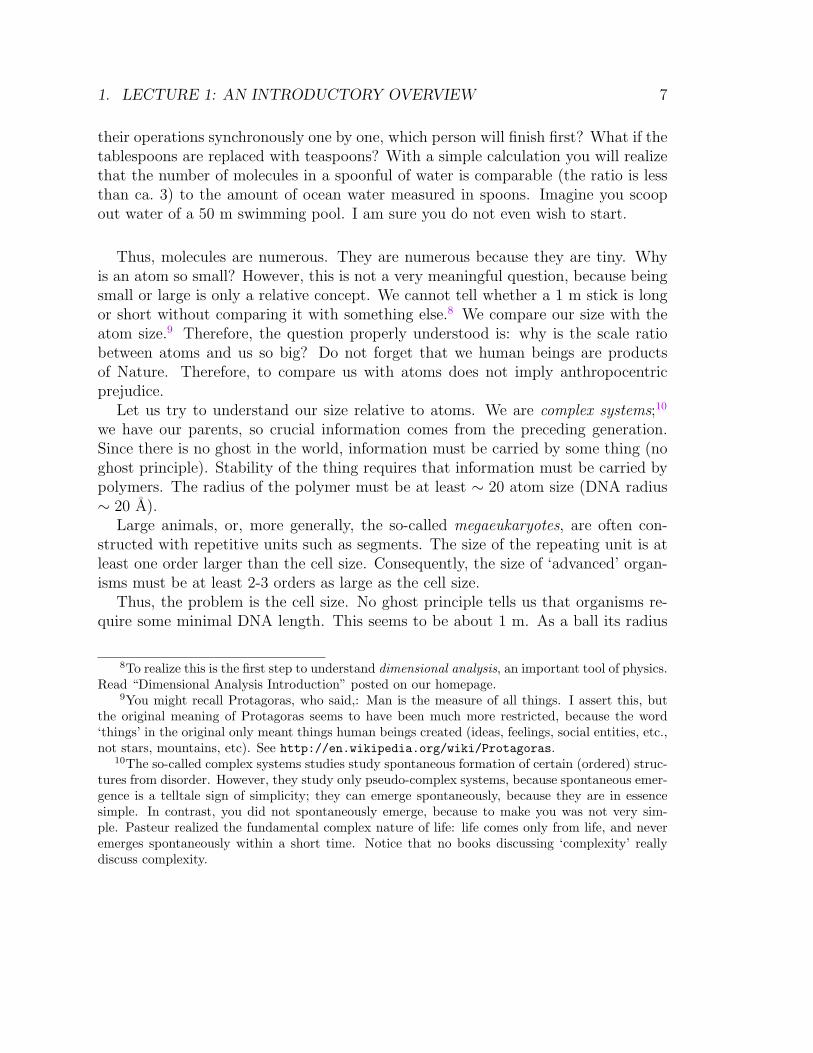
Maxwell clearly recognized that molecules behave erratically due to collisions.Perhaps the simplest model to illustrate the point is the Sinai billiard. A hard ballis moving on the flat table, which has a circular obstacle on it. The ball hit the
11‘Order’ may be understood as redundancy in the world; knowing one thing can tell somethingmore simply because everything is not totally new.
12Here, ‘better’ means it is more favorable to the reproductive success of the organisms.13You will not study if your grade is randomly assigned.14Mistaking correlation as causality is an important ingredient of superstition.
1. LECTURE 1: AN INTRODUCTORY OVERVIEW 9
obstacle and is bounced back specularly (see Fig. 1.1).
Figure 1.1: Sinai billiard: Left: a motivation. Two hard elastic discs (pucks) are running aroundon the table with a periodic boundary condition (= flat torus) colliding from time to time witheach other. This is a toy model of a confined gas. Right: If the dynamic of the center of mass(CM) of one disk is observed from the CM of the other disk, the former may be understood as aballistic motion of a point mass with occasional collisions with the central circular obstacle. Thisis called the Sinai billiard, and is known to be maximally chaotic.
Roughly speaking, a small deviation of the direction of the particle is doubled uponspecular reflection at the central circle, so, for example, to predict the direction of theparticle after 100 collisions is very hard. Imagine what happens if there are numer-ous such particles colliding with each other. Thus, predictions would be absolutelyimpossible. Further worse, it is very hard to exclude the effects of the external world.E. Borel pointed out that the trajectory of a molecule after a very short time can betotally altered, if one gram of mass moves by 1 cm on Sirius (11 ly away from us)due to the change in gravitational field. This implies that you cannot even breath ifyou wish to study the ‘intrinsic behavior’ of a collection of atoms.15
Thus, the microscopic world is full of noise, and everything is stochastic. Kinetictheory handles the microscopic world with space-time local dynamics (collision dy-namics) + statistical assumptions. Even though modern kinetic theory initiated byBoltzmann is a very sophisticated system, it can study only dilute systems. It isalmost hopeless to study condensed matter honestly within kinetic theory, so I willgive only a very elementary introduction to kinetic theory in Chapter 1.
Since the world on the scale of atoms is full of noise, lawfulness requires somescale away from the atomic scale. We know our scale is quite remote from theatomic scale (time scales are also disparate 0.1 fs = 10−16 s). Lawfulness must comefrom suppression of noise. Size is crucial to suppress noise; even if particles in a smalldroplet undergo quite erratic motion, if many particles are averaged, the erratic effect
15Quantum mechanically, subtle entanglements are easily lost by perturbation, so the system isvery fragile.
10 CONTENTS
would disappear: Let Xn be random variables. Then,16
N∑n=1
Xn = Nm+ o[N ], (1.1)
where m is the average value (= expectation value) of Xn. This is the law of largenumbers, the most important pillar of modern probability theory and key to under-standing the macroscopic world. You may imagine outcomes of coin tossing as anexample: Xn = 1 if the nth outcome is a head; otherwise, Xn = 0. By throwing acoin N times, we get a 01 sequence of length N , say, 0100101101110101· · ·001. Youcan guess the sum is roughly N/2. This is the law of large numbers. We clearly seethe importance of being big (relative to atoms).
You might object, however, that being big is not enough; we know violent phe-nomena in the macroscopic world like turbulence or perhaps the core of galaxies. Forregularity to be felt, N in the law of large numbers should not be too big; if you canrealize the regularity of the world after averaging for 1000 generations, probably thelaw of large numbers cannot favor intelligence. Thus, as already discussed above,the world in which intelligence can emerge cannot be too violent. We emerge in theworld which is macroscopic and far away from rapid changes (actually close to nochange from the molecular point of view). We live in the world where space-timescale is not only quite remote from the microscopic world of atoms and molecules,but also the extent of nonequilibrium is not too large.
We need a stable simple laws for feeble minds to work (recall the intelligence mustevolve). Our macroscopic world is so lawful that some of us can even believe in thebenevolence of God.
The macroscopic world close to equilibrium can be described phenomenologicallyby thermodynamics. Here, ‘phenomenologically’ implies that what we observe di-rectly can be organized into a single logical system without assuming any entitiesbeyond direct observations. Thermodynamics is distilled from empirical facts, so itis the most reliable theoretical system we have in physics. Classical mechanics wasdisqualified as a fundamental theory, because it contradicts thermodynamics.
As we will learn statistical mechanics obtains the Helmholtz free energy as
A = −kBT logZ, (1.2)
where kB is the Boltzmann constant, T the absolute temperature, and Z is the
16o: This symbol means higher order smaller quantities. For example, N0.99 is o[N ].
1. LECTURE 1: AN INTRODUCTORY OVERVIEW 11
(canonical) partition function
Z =∑
e−H/kBT . (1.3)
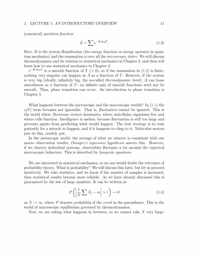
Here, H is the system Hamiltonian (the energy function or energy operator in quan-tum mechanics) and the summation is over all the microscopic states. We will discussthermodynamics and its relation to statistical mechanics in Chapter 2, and then willlearn how to use statistical mechanics in Chapter 3.e−H/KBT is a smooth function of T (> 0), so if the summation in (1.3) is finite,
nothing very singular can happen in A as a function of T . However, if the systemis very big (ideally, infinitely big, the so-called thermodynamic limit), A can loosesmoothness as a function of T ; an infinite sum of smooth functions need not besmooth. Thus, phase transition can occur. An introduction to phase transition isChapter 5.
What happens between the microscopic and the macroscopic worlds? In (1.1) theo[N ] term becomes not ignorable. That is, fluctuation cannot be ignored. This isthe world where Brownian motion dominates, where unicellular organisms live andwhere cells function. Intelligence is useless, because fluctuation is still too large andprevents agents from predicting what would happen. The best strategy is to waitpatiently for a miracle to happen, and if it happens to cling to it. Molecular motorsjust do this, crudely put.
In the mesoscopic world, the average of what we observe is consistent with ourmacro observation results; Onsager’s regression hypothesis asserts this. However,if we observe individual systems, observables fluctuate a lot around the expectedmacroscopic behaviors. This is described by Langevin equations.
We are interested in statistical mechanics, so no one would doubt the relevance ofprobability theory. What is probability? We will discuss this later, but let us proceedintuitively. We take statistics, and we know if the number of samples is increased,then statistical results become more reliable. As we have already discussed this isguaranteed by the law of large numbers. It can be written as
P
(∣∣∣∣ 1
N
∑Xi −m
∣∣∣∣ > ε
)→ 0 (1.4)
as N →∞, where P denotes probability of the event in the parentheses. This is theworld of macroscopic equilibrium governed by thermodynamics.
Now, we are asking what happens in between, so we cannot take N very large.
12 CONTENTS
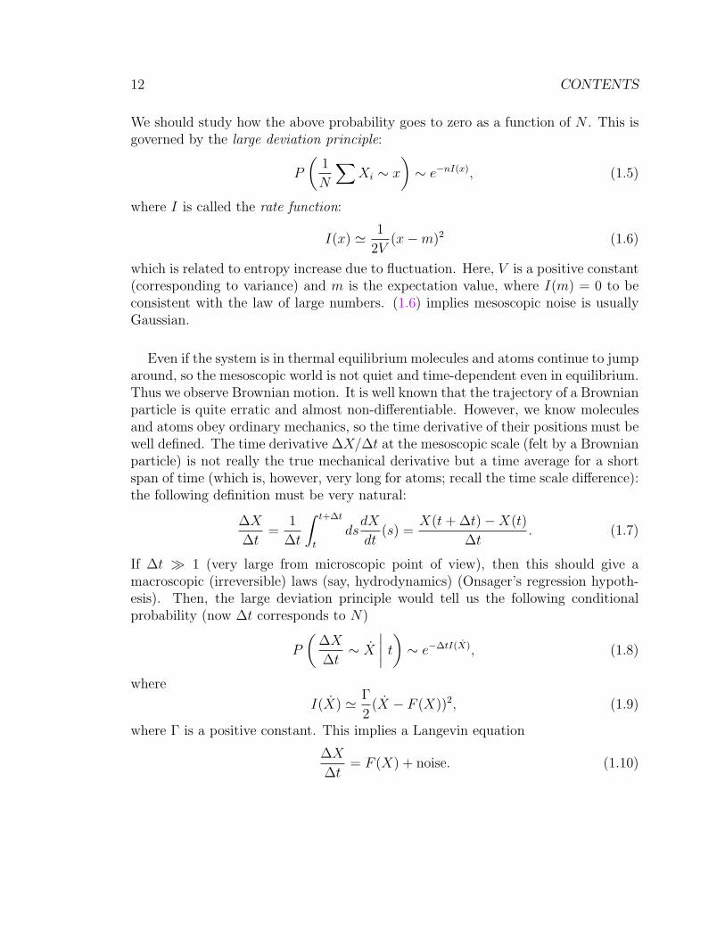
We should study how the above probability goes to zero as a function of N . This isgoverned by the large deviation principle:
P
(1
N
∑Xi ∼ x
)∼ e−nI(x), (1.5)
where I is called the rate function:
I(x) ' 1
2V(x−m)2 (1.6)
which is related to entropy increase due to fluctuation. Here, V is a positive constant(corresponding to variance) and m is the expectation value, where I(m) = 0 to beconsistent with the law of large numbers. (1.6) implies mesoscopic noise is usuallyGaussian.
Even if the system is in thermal equilibrium molecules and atoms continue to jumparound, so the mesoscopic world is not quiet and time-dependent even in equilibrium.Thus we observe Brownian motion. It is well known that the trajectory of a Brownianparticle is quite erratic and almost non-differentiable. However, we know moleculesand atoms obey ordinary mechanics, so the time derivative of their positions must bewell defined. The time derivative ∆X/∆t at the mesoscopic scale (felt by a Brownianparticle) is not really the true mechanical derivative but a time average for a shortspan of time (which is, however, very long for atoms; recall the time scale difference):the following definition must be very natural:
∆X
∆t=
1
∆t
∫ t+∆t
t
dsdX
dt(s) =
X(t+ ∆t)−X(t)
∆t. (1.7)
If ∆t 1 (very large from microscopic point of view), then this should give amacroscopic (irreversible) laws (say, hydrodynamics) (Onsager’s regression hypoth-esis). Then, the large deviation principle would tell us the following conditionalprobability (now ∆t corresponds to N)
P
(∆X
∆t∼ X
∣∣∣∣ t) ∼ e−∆tI(X), (1.8)
where
I(X) ' Γ
2(X − F (X))2, (1.9)
where Γ is a positive constant. This implies a Langevin equation
∆X
∆t= F (X) + noise. (1.10)
1. LECTURE 1: AN INTRODUCTORY OVERVIEW 13
Γ (or rather Γ−1) describes the size of noise, which must be just right to be consis-tent with thermodynamics. Therefore, Γ obeys a certain relation with temperature(fluctuation-dissipation relation). We will look at the introductory part of these top-ics in Chapter 4.
Notice that (1.8) gives the transition probability:
P (X + X∆t, t+ ∆t |X, t) ∼ e−∆tI(X). (1.11)
This leads to a path integral formulation of nonequilibrium phenomena (Onsager-Machlup-Hashitsume formalism)
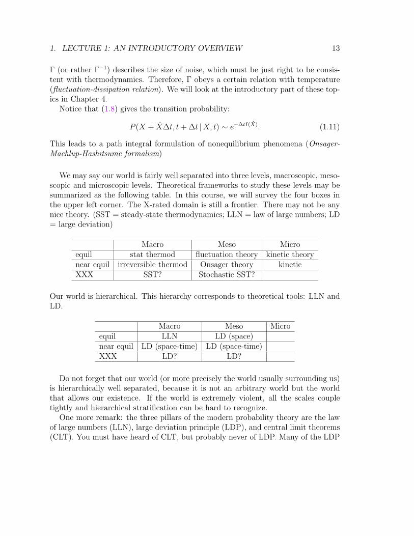
We may say our world is fairly well separated into three levels, macroscopic, meso-scopic and microscopic levels. Theoretical frameworks to study these levels may besummarized as the following table. In this course, we will survey the four boxes inthe upper left corner. The X-rated domain is still a frontier. There may not be anynice theory. (SST = steady-state thermodynamics; LLN = law of large numbers; LD= large deviation)
Macro Meso Microequil stat thermod fluctuation theory kinetic theorynear equil irreversible thermod Onsager theory kineticXXX SST? Stochastic SST?
Our world is hierarchical. This hierarchy corresponds to theoretical tools: LLN andLD.
Macro Meso Microequil LLN LD (space)near equil LD (space-time) LD (space-time)XXX LD? LD?
Do not forget that our world (or more precisely the world usually surrounding us)is hierarchically well separated, because it is not an arbitrary world but the worldthat allows our existence. If the world is extremely violent, all the scales coupletightly and hierarchical stratification can be hard to recognize.
One more remark: the three pillars of the modern probability theory are the lawof large numbers (LLN), large deviation principle (LDP), and central limit theorems(CLT). You must have heard of CLT, but probably never of LDP. Many of the LDP

14 CONTENTS
results are misunderstood as the consequences of CLT (e.g., thermodynamic fluctu-ation theory). For statistical thermodynamics, CLT is most naturally connected tothe renormalization group theory, and it is rare that CLT truly appears in elementarystatistical mechanics.
2. LECTURE 2: ATOMIC PICTURE OF GASES + INTRODUCTION TO PROBABILITY15
2 Lecture 2: Atomic picture of gases + Introduc-
tion to Probability
Summary∗ Gay-Lussac gave key empirical facts: PV ∝ T , law of constant temperature (for
adiabatic free expansion) and law of combining volume.∗ Bernoulli related temperature and kinetic energy of molecules, but to make kinetic
theory precise, we need probability.∗ Probability is essentially the volume of our confidence measure in 0-1 scale. Prob-
ability must satisfy additivity. Gamble called survival race forces subjective prob-ability to agree with empirical probability.
∗ Understand how to describe events in terms of sets.
Key wordsLaw of partial pressure, Joule-Thomson experiment, equipartition of energy, proba-bility, elementary event, sample space, event, conditional probability
What you should be able to do17
∗ Explain the law of constant temperature.∗ Explain why the Joule-Thomson experiment could kill Newton’s repulsive force
model of gases.
According to Aristotelian physics, the four properties, hot, cold, dry and wetwere irreducible properties, which corresponded to four elements of Empedocles,fire, water, earth and air, respectively. The essence is that what we observe directlyby our sense has a direct materials basis.
This type of ideas is called ‘thingification’ or ‘reification.’ Chemistry was naturallyunder its spell; one might say the genomic biology is struggling to emancipate itselffrom this (→1.1.1).
Even Galileo (1564-1642) was initially under this influence, but later he clearlyestablished the mechanical view of Nature, asserting that what we could feel (e.g.,color, odor, etc.) existed only in the relation between the sensing subjects and the
17This summarizes what you should be able to do in practice. Most things required in this courseare practical.
16 CONTENTS
sensed objects and was thus subjective and secondary; only the (geometrical) shapes,numbers, configurations (positions) and movements (position changes) of substanceswere objective and were primary properties.
Mechanics was a key element to overcome this habit of thought.Then, you might thing Galileo could have invented a kinetic theory of gases andcould have conceived warmth as ‘thermal motion.’ This is ‘partially’ correct.
Galileo conceived a special substance ‘fire particles,’ whose vigorous motion wasregarded heat/warmth. I guess he wished to distinguish ‘microscopic motion’ from‘macroscopic motion,’ because he did not know heat engine. The relation betweenmotion and heat was in a certain sense recognized from the fire arms, but the ordinarymotions and motions of bullets may not have been identified.
Boyle (1627-1691) was the first to accept the principle that matter and motionwere the primary things, and was truly free from the Aristotelian ‘reificationism.’He correctly asserted that there were microscopic and macroscopic motions. Theformer was sensed as heat but could not be sensed by us as motion; the only motionwe could sense as such was the ‘progressive motion of the whole’ (i.e., the systematicmotion), which could not be felt by us as warmth even if it was vigorous. Thus,Boyle paved the way to discuss mutual convertibility of heat and (macroscopic) mo-tion. Boyle was the true pioneer of the motion or the kinetic theory of heat (→1.1.2).
Ancient atomism has two ontological entities, atoms and void (→1.1.3). Thebiggest discovery of modern physics about gases was the discovery of atmosphericpressure and vacuum by Torricelli (1608-1647), Pascal (1623-1662) and von Guericke(1602-1686). This was a discovery demarcating the medieval and modern ages, itsimportance only second to heliocentrism. Do not forget that even Galileo explainedthe impossibility of sucking water higher than 10 m by the competition of gravityand the abhorrence of vacuum by air.
Within the Aristotelean system, air and fire were regarded essentially light ele-ments, having the tendency to go away from the earth. Therefore, the idea of mass(or weight) of air could not be born. The discovery of vacuum decisively discreditedAristotle.
Thus, a modern dynamic atomic theory should be possible at any time, and indeed,
2. LECTURE 2: ATOMIC PICTURE OF GASES + INTRODUCTION TO PROBABILITY17
Daniel Bernoulli’s (1700-1782) gas model18 (173819) was the first fully kinetic model.We will discussed a simplified version (ignoring the size of atoms) in a modern fashionshortly.
However, the success of Newtonian mechanics almost derailed atomism based onmechanics. Bernoulli’s work was forgotten for 100 years.
Newton tried to explain Boyle’s law (i.e., PV = constant) in terms of (repulsive)forces acting between particles (→1.1.4). The idea of forces among particles was anovel idea actually deviating from the tradition of mechanistic theories. For New-ton’s contemporary scientists (and also for himself), introduction of gravitationalforce that explains the solar system was so impressive that the take-home lesson ofthe Newton’s success was a program to find forces that explain various phenomena;Newton wrote in author’s preface to Principia, “I wish we could derive the rest ofthe phenomena of nature by the same kind of reasoning from mechanical principles;for I am induced by many reasons to suspect that they may all depend upon certainforces by which the particles of bodies, by some causes hitherto unknown, are eithermutually impelled towards each other, and cohere in regular figures, or are repelledand recede from each other; which forces being unknown, philosophers have hithertoattempted the search of nature in vain; but I hope the principles here laid down willafford some light either to this or some truer method of philosophy.”20
Crudely put, somehow, Galileo’s fire particle, Newton’s ether (→1.1.5),21 the‘pure elemental fire’ of Boerhaave (1668-1738) were understood as analogues. New-ton’s repulsive (springy) molecules were imagined due to the clouds of such particlessurrounding the molecules. In any case for about 100 years, this Newton’s programstifled the kinetic attempts. However, between Daniel Bernoulli (ca 1740) and themodern kinetic theory (due to Maxwell (1831-1879) ca 1860) was the general accep-tance of chemical atomic theory (ca 1810) and the birth of physics in the modernsense.
Also between 1740 (D. Bernoulli’s theory) and 1860 (Maxwell’s theory) crucialempirical facts were accumulated, making kinetic theory almost the sole explanation
18This was in his book on hydrodynamics.19J S Bach, Mass in B minor (BWV 232) was the same year.20Principia author’s preface (May 8, 1686).21Newton’s philosophical starting point was New Platonism of Cambridge and Alchemy; both
presupposed that the world is activated by the active principle. Ether was understood as theprotoplast created by God to ‘entrust’ His own activity. Initially, Newton conceived a pan-etherialcosmology.

18 CONTENTS
of gasses (→1.1.7).Dalton (1766-1844) asserted the law of partial pressure:22 the total pressure of a
gas mixture is simply the sum of the pressures each kind of gas would exert if it wereoccupying the space by itself. As illustrated in Fig. 2.1, it is very naturally explainedfrom the atomic point of view.
+=
P = P + P P PA B BA
Figure 2.1: The law of partial pressure due to Dalton
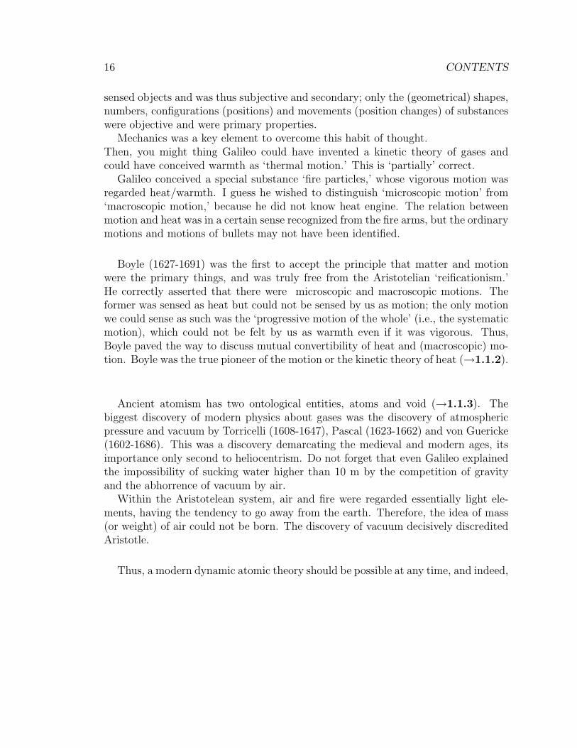
Gay-Lussac (1778-1850) then established three important laws (ca 181023):(i) The law of thermal expansion of gases (also called Charles’ law; P ∝ T if V isconstant).(ii) The law of constant temperature under adiabatic expansion: if a gas is suddenlyallowed to occupy a much larger space by displacing a piston, there is practically notemperature change. You can simulate this nicely using http://www.falstad.com/gas/.(iii) the law of combining volume: in gas phase reactions the volumes of reactants andproducts are related to each other by simple rational ratios implying that ‘particles’cannot generally be atoms.24
At last in 181125 Avogadro (1776-1856) proposed Avogadro’s hypothesis: every gascontains the same number of molecules at the same pressure, volume, and temper-ature. However, the molecular theory was not generally accepted until 1860, whenCannizzaro (1826-1910) presented it to the Karlsruhe Congress (However, Clausiusaccepted this by 1850;26 actually, Cannizzaro mentioned Clausius.27).
22Dalton arrived at his atomic theory not very inductively as is stressed by Brush on p32;Dalton’s writings are sometimes hard to comprehend due to arbitrary thoughts and their outcomesbeing nebulously mixed up with real experimental results (Yamamoto loc. cit. p194), quite differentfrom well-educated Gay-Lussac.
23[1860: Napoleon married Marie Louise of Austria] Notice that Gay-Lussac was the first gener-ation of professional scientist trained professionally to be a scientist. He was a product of FrenchRevolution.
24But Dalton rejected this interpretation, saying, e.g., Gay-Lussac’s experiments were inaccurate,etc. This clearly indicates that Dalton was a metaphysicist more than a physicist.
25[1811: J Austin published Sense and Sensibility]26Brush p5127C. Cercignani, “The rise of statistical mechanics,” in Chance in Physics, Lect. Notes Phys.
2. LECTURE 2: ATOMIC PICTURE OF GASES + INTRODUCTION TO PROBABILITY19
+ =
H O H O22 2
Figure 2.2: The law of combining volume indicating that generally gases are made of moleculesinstead of atoms. The figure illustrates 2H2 + O2 → 2H2O.
P1 2P
P1
2
2P
V1 V
final stateinitial state
porous plug
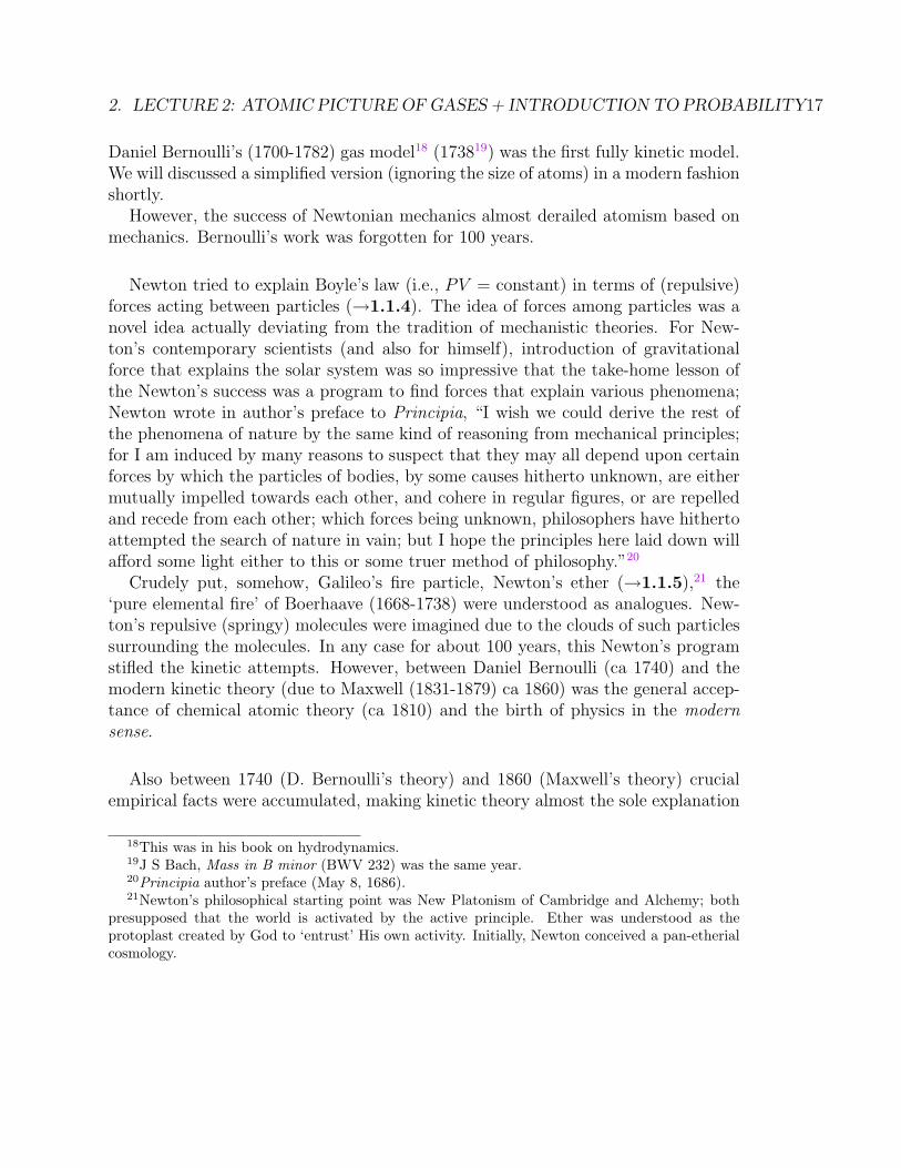
Figure 2.3: The throttle experiment by Joule and Thomson; initially a gas is in the right withvolume V1. At the end the gas is in the left with volume V2.
The Joule-Thomson experiment was performed in 1852-4 (→1.1.9). A gas in thestate of pressure P1 and volume V1 is pushed out through a porous plug (e.g., cottonplug) into the one in the state of pressure P2 and volume V2 gently under thermalinsulation (no exchange of heat). The process is called the Joule-Thomson process(or throttling process), and the temperature change due to this process is called theJoule-Thomson effect. The idea of this experiment is to check whether the kineticenergy of the gas (i.e., temperature) is conserved or not through this process.
Since we can know the work W applied to the gas during the process as W =P1V1−P2V2, and since there is no other energy input nor output. We can, in partic-ular, choose V1 < V2 but W = 0. If the temperature of the gas changes, this impliesthere must be a potential energy among gas particles.
In many cases around the room temperature, the temperature decreases with thethrottling process. This implies that there is an attractive interactions among gasparticles. So molecular forces are attractive, and Newton was killed.
Let us look at Daniel Bernoulli’s work (→1.1.11). The (kinetic interpretation of)pressure on the wall is the average momentum given to the wall per unit time and
574 (edited by J. Bricmont, D. Durr, M. C. Gallavotti, G. C. Ghirardi, F. Petruccione and N.Zanghi) p25 (2001). This article gives a good summary of Boltzmann’s progress.
20 CONTENTS
area by
x
wall
vx
vx−
Impulse given to wall
= 2m vx
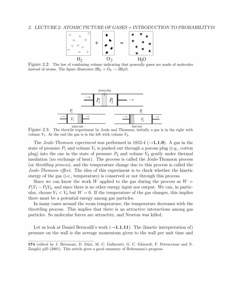
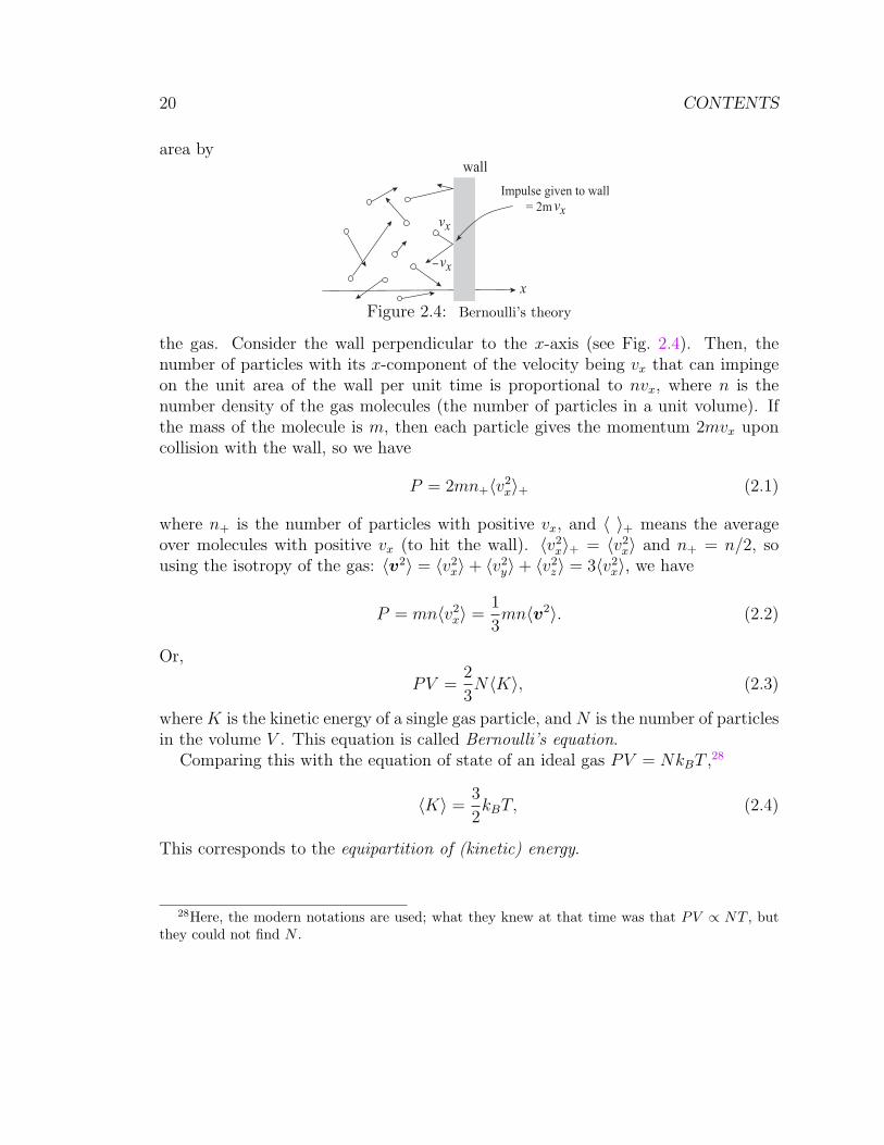
Figure 2.4: Bernoulli’s theory
the gas. Consider the wall perpendicular to the x-axis (see Fig. 2.4). Then, thenumber of particles with its x-component of the velocity being vx that can impingeon the unit area of the wall per unit time is proportional to nvx, where n is thenumber density of the gas molecules (the number of particles in a unit volume). Ifthe mass of the molecule is m, then each particle gives the momentum 2mvx uponcollision with the wall, so we have
P = 2mn+〈v2x〉+ (2.1)
where n+ is the number of particles with positive vx, and 〈 〉+ means the averageover molecules with positive vx (to hit the wall). 〈v2
x〉+ = 〈v2x〉 and n+ = n/2, so
using the isotropy of the gas: 〈v2〉 = 〈v2x〉+ 〈v2
y〉+ 〈v2z〉 = 3〈v2
x〉, we have
P = mn〈v2x〉 =
1
3mn〈v2〉. (2.2)
Or,
PV =2
3N〈K〉, (2.3)
where K is the kinetic energy of a single gas particle, and N is the number of particlesin the volume V . This equation is called Bernoulli’s equation.
Comparing this with the equation of state of an ideal gas PV = NkBT ,28
〈K〉 =3
2kBT, (2.4)
This corresponds to the equipartition of (kinetic) energy.
28Here, the modern notations are used; what they knew at that time was that PV ∝ NT , butthey could not find N .
2. LECTURE 2: ATOMIC PICTURE OF GASES + INTRODUCTION TO PROBABILITY21
Let us rederive the equipartition of kinetic energy in another elementary fashion(→1.1.13). As we will learn, calculating the partition function Z, we can systemat-ically derive this in a very streamlined fashion. Although it is very important thatyou can drive a fancy sport car on highways, you should also be able to walk.
Consider a two particle collision process. In equilibrium,
〈w · V 〉 = 0, (2.5)
where w is the relative velocity and V is the center of mass velocity. If we writethese in terms of the velocities of two particles v1 and v2 and their respective massesm1 and m2, we have
w · V =(v1 − v2) · (m1v1 +m2v2)
m1 +m2
=(m1v
21 −m2v
22) + (m2 −m1)v1 · v2
m1 +m2
. (2.6)
We know 〈v1 · v2〉 = 0, so we get the equality of the average kinetic energies. Wecan conclude that even if the masses of particles are all different, we get the sameideal gas law.
Question. We have demonstrated the equipartition law, but we can give any initialcondition to the gas. Do you believe that the equipartition law eventually holds evenif the initial condition does not satisfy the law? ut
To go beyond Bernoulli and these elementary discussions, we need the idea ofprobability. When Maxwell was 19 years old, he read an article introducing the con-tinental statistical theory into British science (e.g., Gauss’s theory), and was reallyfascinated by it. He wrote to his friend: “the true logic for this world is the Calculusof Probabilities · · ·.”29
I will give an introduction to measure-theoretical probability theory (→Section 1.2),although no formal introduction of measures will be discussed. You can simply un-derstand that a ‘measure’ is a precise concept corresponding to volumes and weights.
Suppose we have a jar containing 5 white balls and 2 black balls (→1.2.1). Whatis the degree Cw on the 0-1 scale of your confidence for you to pick a white ball outof the jar? We expect that, on the average, 5 times out of 7 we will take a white ballout. Hence, it is sensible to say that our confidence in the above statement is 5/7 onthe 0-1 scale.
29Brush p59
22 CONTENTS
Figure 2.5: Take out one ball without looking in the jar with replacement. How are you sureyou get a white ball?
Suppose you gain one dollar if you pick up a black ball, but you must pay X dollars,otherwise. If X is too large you will not participate in this gamble. What is therational choice for you? If your expected gain
(1− Cw)−XCw ≥ 0 (2.7)
is non-negative, it is sensible for you to play this game: X ≤ 1/Cw − 1. In this way,your confidence level matters if you wish to survive in this world. Here, it is notguaranteed that your Cw is realistic. If not realistic, you must pay the price. In anycase, a lesson we have learned is by gambling, you can tell whether your belief isright or not.
What do we mean when we say that there will be 70 % chance of rain tomorrow?In this case, in contrast to the preceding example, we cannot repeat tomorrow againand again. However, the meaning seems clear. Again, you could devise a gamblingdependent of the weather.
To make a mathematical theory, we must describe events as sets (→1.2.2). Anevent which cannot (or need not) be analyzed further into a combination of eventsis called an elementary event. For example, to rain tomorrow is an elementary event(if you ask whether you prepare for rain gear), but to rain or to snow tomorrow isa combination of two elementary events. An elementary event need not be an eventno one can dissect further. If you wish to use in a game not only the faces but alsothe directions of the edges of a dice, then your elementary events are not only facesbut faces and directions combined. Of course, that is not often the case, and usuallywe pay our attention only to the faces, so faces 1, 2, · · · , 6 are the elementary eventsfor a dice.
Denote by Ω the totality of elementary events (called the sample space) allowedin the situation or to the system under study. Any (compound) event under consid-eration can be identified with a subset of Ω.
When we say an event corresponding to a subset A of Ω occurs, we mean that oneof the elements in A occurs.
2. LECTURE 2: ATOMIC PICTURE OF GASES + INTRODUCTION TO PROBABILITY23
a
bc
e
s
tv
wx
y
z
.
..
.
.
.
.
Ω
A
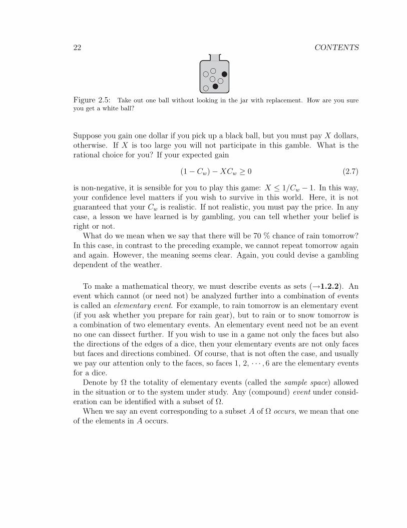
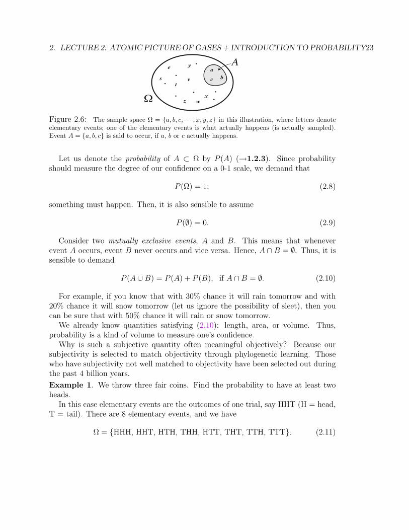
Figure 2.6: The sample space Ω = a, b, c, · · · , x, y, z in this illustration, where letters denoteelementary events; one of the elementary events is what actually happens (is actually sampled).Event A = a, b, c is said to occur, if a, b or c actually happens.
Let us denote the probability of A ⊂ Ω by P (A) (→1.2.3). Since probabilityshould measure the degree of our confidence on a 0-1 scale, we demand that
P (Ω) = 1; (2.8)
something must happen. Then, it is also sensible to assume
P (∅) = 0. (2.9)
Consider two mutually exclusive events, A and B. This means that wheneverevent A occurs, event B never occurs and vice versa. Hence, A ∩B = ∅. Thus, it issensible to demand
P (A ∪B) = P (A) + P (B), if A ∩B = ∅. (2.10)
For example, if you know that with 30% chance it will rain tomorrow and with20% chance it will snow tomorrow (let us ignore the possibility of sleet), then youcan be sure that with 50% chance it will rain or snow tomorrow.
We already know quantities satisfying (2.10): length, area, or volume. Thus,probability is a kind of volume to measure one’s confidence.
Why is such a subjective quantity often meaningful objectively? Because oursubjectivity is selected to match objectivity through phylogenetic learning. Thosewho have subjectivity not well matched to objectivity have been selected out duringthe past 4 billion years.
Example 1. We throw three fair coins. Find the probability to have at least twoheads.
In this case elementary events are the outcomes of one trial, say HHT (H = head,T = tail). There are 8 elementary events, and we have
Ω = HHH, HHT, HTH, THH, HTT, THT, TTH, TTT. (2.11)

24 CONTENTS
The word “fair” means that all elementary events are equally likely. Hence, theprobability of any elementary event should be 1/8. The event A, defined by havingat least 2 H’s, is given by A = HHH, HHT, HTH, THH. Of course, elementaryevents are mutually exclusive, so P (A) = 1/2. ut
As can be seen from this example, estimating probability is often closely relatedto counting the number of combinations. See Appendix to Section 1.2 of the Lecturenotes.
Suppose a shape is drawn in a square of area 1 (→1.2.4). If we pepper it withpoints uniformly, then the probability = our confidence level of a point to land onthe shape should be proportional to its area.30 Thus, again it is intuitively plausiblethat probability and area or volume are closely related.
A
Figure 2.7: Peppering the unit square evenly with points, we can estimate the area of A.
A particular measure of the extent of confidence may be realistic or unrealistic(rational or irrational), but this is not the concern of probability theory. Proba-bility theory studies the general properties of the confidence level of an event thatmathematically behaves as a normalized measure (= volume or weight).
Defined as the level of confidence, isn’t probability only subjective? (→1.2.6) Howcan we use it to do objective science? We know the objective probability is forcedupon us by selection (evolution process), so may probabilities are virtually objec-tive. However, to be useful in quantitative science, objective probabilities should beactually measured by experiments. To this end, we must review a bit of elementaryprobability theory.
Let us begin with elementary facts (→1.2.7). It is easy to check that
P (A ∪B) ≤ P (A) + P (B), (2.12)
A ⊂ B ⇒ P (A) ≤ P (B). (2.13)
30This has a practical consequence. See Lecture 3.
2. LECTURE 2: ATOMIC PICTURE OF GASES + INTRODUCTION TO PROBABILITY25
Denoting Ω \ A by Ac (complement), we get
P (Ac) = 1− P (A). (2.14)
Suppose we know for sure that event B has occurred. Under this condition whatis the probability of the occurrence of the event A? Thus we need the concept ofconditional probability (→1.2.8). We write this conditional probability as P (A|B),and define it through
P (A|B) =P (A ∩B)
P (B), (2.15)
so that P (B |B) = 1 should hold.
26 CONTENTS
3 Lecture 3: Law of large numbers
Summary∗ The law of large numbers allows us to measure probability.∗We can use the law of large numbers to estimate integrals. Recognize the power of
randomness.
Key words(Statistical) independent event, stochastic (random) variable, expectation value, vari-ation, standard deviation, indicator, statistical independence of random variables,Chebyshev’s inequality, law of large numbers
What you should be able to do∗ Be able to calculate expectation values and variations for simple cases.∗ Understand P (A) = 〈χA〉.∗ You must be able to use the law of large numbers to estimate how many samples
you need to determine the empirical average with a prescribed error tolerancelevel.
We discussed molecular nature of gas and studied average kinetic energy: We ob-tained the equipartition of energy. There was a discussion in the lecture notes: doesthe law hold in 1d? Think.
We have started discussing probability:∗ Event A may be understood as a subset of the sample space Ω, the totality of whatcan happen (the basic event that actually happens is called the elementary event). IfA = a, b, c, d, where a, · · · , d are elementary events, occurs, one of a, · · · , d actuallyoccurs. →1.2.2.∗ Probability is a measure (volume) of your confidence in the occurrence of a partic-ular event A. Additivity holds and P (Ω) = 1. →1.2.3. For example,
P (A ∪B) = P (A) + P (B)− P (A ∩B), (3.1)
When the occurrence of event A does not tell us anything new about event B andvice versa, we say the two events A and B are (statistically) independent. Do notconfuse ‘independent events’ and ‘mutually exclusive events.’ Since knowing about
3. LECTURE 3: LAW OF LARGE NUMBERS 27
the event B does not help us to obtain more information about A if A and B areindependent, we should get
P (A|B) = P (A), (3.2)
where P (A |B) = P (A ∩ B)/P (B) is the conditional probability we already in-troduced. Therefore, the following formula must be an appropriate definition ofindependence of events A and B:
P (A ∩B) = P (A|B) · P (B) = P (A) · P (B). (3.3)
For example, when we use two fair dice ‘a’ and ‘b’ and ask the probability for ‘a’to exhibit a number less than or equal to 2 (event A), and ‘b’ a number larger than3 (event B), we have only to know the probability for each event A = 1, 2 andB = 4, 5, 6. Thus, the answer is P (A∩B) = P (A) ·P (B) = 1/3 · 1/2 = 1/6.
You must have heard of ‘stochastic processes.’ A stochastic process is a processin which a stochastic variable takes various values as a function of time.
Let Ω be the sample space and a probability P is defined on it.31 Then, a function(map) from Ω to some mathematical entity (real numbers, vectors, etc.) is called astochastic variable or random variable.
Suppose Ω = ωi. Then, a real stochastic variable F is a map F : Ω → R.The probability for F to take a value f may be written as P (ω |F (ω) = f) =P (F−1(f)).
For example, if you cast a dice (Ω = 1, 2, 3, 4, 5, 6), and you obtain $1 if theface is odd; otherwise, you must pay $1. Then, your gain f is a random variablef : Ω→ −1,+1 such that f(even face) = −1 and f(odd face) = +1.
If a probability P is specified on Ω, and a stochastic variable F is defined on it,then we know everything we can know about the probabilistic properties of F . Forexample, we know the probability PF (f) for F = f for any f in its range. However,in reality, to determine these probabilities in detail is not very easy. Thus, we wishto represent PF with a couple of numbers.
The expectation value (= average) (→1.2.11) of F with respect to the probabilityP is written as EP (F ) or 〈F 〉P and is defined by
EP (F ) ≡ 〈F 〉P ≡∑ω∈Ω
P (ω)F (ω) =∑
f
PF (f)f. (3.4)
31(Ω, P ) is called a probability space. If you read a respectable probability book, you will en-counter something like (Ω,B, P ), where B is a family of ‘measurable sets.’ We will not discuss thisin these notes. (Not all the events should have probabilities to avoid something like 1 + 1 = 3, sowe must specify what events can have probabilities. This is the role of B.)
28 CONTENTS
Often the suffix P is omitted.The sum becomes integration when we study events which are specified by a
continuous parameter. In this case,
EP (F ) ≡ 〈F 〉P ≡∫
ω∈Ω
F (ω)dP (ω) =
∫ω∈Ω
F (ω)P (dω), (3.5)
where P (dω) is the probability of the volume element dω (often P (dω) is written asdP (ω)). You may simply interpret this integral just as the Riemann integral.E is a linear operator: Suppose f and g are stochastic variables, and a and b are
real numbers. Then, E(af + bg) = aE(f) + bE(g).
We are also interested in the ‘spread’ of the variables. Its good measure is thevariance of X defined as
V (X) = E([X − E(X)]2) = E(X2)− E(X)2. (3.6)
Its square root σ(X) =√V (X) is called the standard deviation of X.
The indicator χA of a set (= event in our context) A is defined by
χA(ω) ≡
1 if ω ∈ A,0 if ω 6∈ A. (3.7)
This indicates the answer ‘yes’ or ‘no’ to the question: does the event A happen?Notice that (apply (3.4) straightforwardly)
〈χA〉P =∑
ω
χA(ω)P (ω) =∑ω∈A
P (ω) = P (A). (3.8)
This is a very important relation for the computation of probabilities.A random variable X defined on Ω may be written as
X(ω) =∑ω∈Ω
xχω |X=x(ω). (3.9)
This is of course consistent with (3.4):
〈X(ω)〉 =∑ω∈Ω
x〈χω |X=x(ω)〉 =∑
x
xPX(x), (3.10)
where PX(x) is the probability for X to be x
3. LECTURE 3: LAW OF LARGE NUMBERS 29
How should we define ‘independence’ (statistical independence) of two stochasticvariables X1 and X2? A reasonable answer is that
E(f(X1)g(X2)) = E(f(X1))E(g(X2)) (3.11)
holds for any functions32 f and g of the stochastic variables. In particular, if stochas-tic variables X1 and X2 are independent,
E(X1X2) = E(X1)E(X2). (3.12)
Why is (3.11) reasonable? The event F = a and G = b should be statistically independentfor any (admissible) values a and b. This requires (notice that χAχB = χA∩B ; see (3.3) and(3.8))
E(χω |F=aχω |G=b) = E(χω |F=a)E(χω |G=b) (3.13)
for any a and b. If (3.13) holds, then (3.11) holds and vice versa; to get (3.13) from (3.11) we needthe latter to hold for any f and g, because
f(F (ω)) =∑ω∈Ω
χω |F=af(a). (3.14)
That is, virtually any linear combination of χω |F=a can be constructed by choosing f appropri-ately.
If random variables X and Y are independent, then
V (X + Y ) = V (X) + V (Y ). (3.15)
[This I did not discuss in the class] If you have more than two random variables,you might wish to know their relations. For two stochastic variables X and Y
C(X, Y ) = E([X − E(X)][Y − E(Y )]) = E(XY )− E(X)E(Y ) (3.16)
is called the covariance between X and Y , which shows up often when we wish tostudy fluctuations.
If X and Y are independent variables, then C(X, Y ) = 0, but the converse is nottrue. Let Y = ±X, where ± is randomly chosen by coin-tossing. Then, C(X, Y ) = 0,but X2 = Y 2, so they cannot be statistically independent.
Suppose χA is the indicator of the area A in the unit square. We pepper dotson it evenly. If the ith dot (location xi) is on A, χA is 1, otherwise, 0. If we count
32‘Any functions’ here means ‘any (Lebesgue) integrable functions.’
30 CONTENTS
the number N1 of 1’s in the total trial of N dots, N1/N should be close to the area,which is the probability P for the dot to land on the area of A. We expect
1
N
N∑i=1
χA(xi)→ E(χA) = P (A) (3.17)
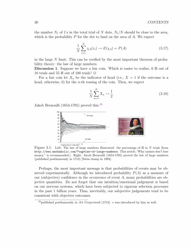
in the large N limit. This can be verified by the most important theorem of proba-bility theory: the law of large numbers.Discussion 1. Suppose we have a fair coin. Which is easier to realize, 6 H out of10 trials and 55 H out of 100 trials? ut
For a fair coin let Xn be the indicator of head (i.e., X = 1 if the outcome is ahead, otherwise, 0) for the n-th tossing of the coin. Then, we expect
1
N
N∑n=1
Xn →1
2. (3.18)
Jakob Bernoulli (1654-1705) proved this.33
N
Figure 3.1: Left: The law of large numbers illustrated: the percentage of H in N trials [fromhttp://www.mathaholic.com/?tag=law-of-large-numbers. This article, ‘Why casinos don’t losemoney,” is recommended.]. Right: Jacob Bernoulli (1654-1705) proved the law of large numbers(published posthumously in 1713) [Swiss stamp in 1994].
Perhaps, the most important message is that probabilities of events may be ob-served experimentally. Although we introduced probability P (A) as a measure ofour (subjective) confidence in the occurrence of event A, many probabilities are ob-jective quantities. Do not forget that our intuition/emotional judgement is basedon our nervous systems, which have been subjected to rigorous selection processesin the past 1 billion years. Thus, inevitably, our subjective judgements tend to beconsistent with objective outcomes.
33published posthumously in Art Conjectandi (1713). e was introduced by him as well.
3. LECTURE 3: LAW OF LARGE NUMBERS 31
The following URL illustrates the law of large numbers:http://demonstrations.wolfram.com/IllustratingTheLawOfLargeNumbers/
You will realize that convergence is not very fast.
A precise statement of the law of large numbers (LLN) is as follows:Let Xi be a collection of independently and identically distributed (often abbrevi-ated as iid) stochastic variables. For any ε > 0,
limN→∞
P
(∣∣∣∣∣ 1
N
N∑n=1
Xn − E(X1)
∣∣∣∣∣ > ε
)= 0 (3.19)
holds under the condition that the distribution of Xi is not too broad: E(|X1|) <∞.If V (X1) < +∞, the condition is satisfied.34 In the following, the law of largenumbers is demonstrated under this assumption.
The following is also a precise expression:
N∑n=1
Xn = NE(X1) + o[N ]. (3.20)
The interpretation of (3.19) is as follows: we perform a series of N experiments toproduce the partial sum
∑n xn. This set of N experiments is understood as a single
‘run,’ and we imagine many such runs. Then, (3.19) tells us that the probabilitythat these runs produce empirical averages deviated from the true mean by ε goesto zero in the limit of the infinite run length.Remark: If you make a partial sum SN =
∑Nn=1Xn and compute an empirical
average SN/N , this may be larger than E(X1). Then, you might guess that thereshould be more chance to have values to compensate this deviation (i.e., you wouldexpect more outcomes smaller than E(X1) in the near future), but this is the famousgambler’s fallacy (or fallacy of the maturity of chances). Seehttp://en.wikipedia.org/wiki/Gambler’s_fallacy, especially, psychology be-hind the fallacy. ut
Before going to a rigorous demonstration of LLN, let us understand why it isplausible. We could expect that the average of SN/N (the empirical average) shouldfluctuate around E(X1). Its width of fluctuation must be evaluated by the variance:
34Since all Xn are distributed identically, we use X1 as a representative, so E(X1), etc., showup in the statement.
32 CONTENTS
(notice that V (cX) = c2V (X) and (3.15))
V
(1
N
N∑n=1
Xn
)=
1
N2V
(N∑
kn=1
Xn
)=
1
N2
N∑n=1
V (Xn) =1
NV (X1). (3.21)
Thus, the width of the distribution shrinks as N is increased. That is why SN/Nclusters tightly around E(X1) as N →∞. This is the essence of LLN. This is illus-trated in:http://demonstrations.wolfram.com/ChebyshevsInequalityAndTheWeakLawOfLargeNumbersForIidTwoVect/
The key to an honest proof of LLN is Chebyshev’s inequality35
a2P (|X − E(X)| ≥ a) ≤ V (X). (3.22)
This can be shown as follows (let us redefine X by shifting as X−E(X) to get rid ofE(X) from the calculation).36 We start from the definition of the variance (→1.2.18for an illustration of the following estimates):
V (X) =
∫X2dP (ω). (3.23)
Here, the integration range is over all values of X. Now, let us remove the range|X| < a from this integration range. The integrand is positive, so obviously∫
X2dP (ω) ≥∫|X|≥a
X2dP (ω). (3.24)
On the integration range |X| ≥ a, X2 ≥ a2, so∫|X|≥a
X2dP (ω) ≥∫|X|≥a
a2dP (ω) = a2
∫|X|≥a
dP (ω). (3.25)
This impliesV (X) ≥ a2P (|X| ≥ a). (3.26)
Since we have shifted X by E(X), this implies Chebyshev’s inequality (3.22).
35In the following the assertion is proved under a stronger condition that V (X) is finite. Toprove the law under the condition E(|X1|) <∞ requires some tricks.
36Or, you can use V (X) = V (X − a) for any number a; the width does not change wherever thedistribution is placed.
3. LECTURE 3: LAW OF LARGE NUMBERS 33
We wish to apply Chebyshev’s inequality (3.22) to the sample average (1/N)∑Xn.
Replacing corresponding quantities in (3.22) (X → (1/N)∑Xn, a → ε), and using
(3.21), we get
P
(∣∣∣∣∣ 1
N
N∑n=1
Xn − E(X1)
∣∣∣∣∣ ≥ ε
)≤ V (X1)
ε2N. (3.27)
Taking N →∞ we arrive at LLN.
Now, we have shown that indeed (3.17) can be used to observe the probabilityof an event. How many times should we throw a coin to check its fairness? Theempirical probability for Head is given by NH/N , where N is the total number oftrials and NH the number of trials resulting in Head. The expectation value of NH/Nis the probability of Head pH . Let Xi be the indicator of the Head event for the i-th trial. Its expectation value is also pH and NH =
∑iXi. Let V (≤ 1/4) be its
variance. Then, the Chebyshev inequality (3.27) implies
P (|NH/N − pH | ≥ ε) ≤ V
ε2N. (3.28)
Therefore, the more unfair the easier to find the fact (because V = pH − p2H), but,
for example, 10% unfairness is not very easy to detect.Perhaps it is fun to simulate the experiments described above computationally,
but if you wish to do it, wait till you learn the large deviation.
Let us consider the problem of numerically evaluating a high-dimensional integral(the Monte-Carlo integration method):
I =
∫ 1
0
dx1 · · ·∫ 1
0
dx1000f(x1, · · · , x1000). (3.29)
If we wish to sample (only) two values for each variable, we need to evaluate thefunction at 21000 ∼ 10300 points (you should remember 210 ' 103). Such sampling isof course impossible.
This integral can be interpreted as the average of f over a 1000 dimensional unitcube:
I =
∫ 1
0dx1 · · ·
∫ 1
0dx1000f(x1, · · · , x1000)∫ 1
0dx1 · · ·
∫ 1
0dx1000
. (3.30)
34 CONTENTS
Therefore, randomly sampling the points rn in the cube, we can obtain
I = limN→∞
1
N
N∑n=1
f(rn). (3.31)
How many points should we sample to estimate the integral within 10−2 error, if weallow larger errors at most once out of 1000 such calculations? We can readily knowthe answer from (3.27): V (f(X1))107. The variance of the value of f is of ordermax |f |2, a constant. Compare this number with 10300 above and appreciate thepower of randomness. This is the principle of the Monte Carlo integration. Noticethat the computational cost does not depend on the dimension of the integral.
How fast or slow the convergence of this method is may be felt from the estimationof π by peppering a disk:http://demonstrations.wolfram.com/MonteCarloEstimateForPi/
In elementary probability courses, you are often asked to answer many combina-torial questions. How to count is a very interesting mathematics, but has no directlogical relation to probability, so we will not discuss the topic here. If you wish toreview its very rudimentary portion, see Appendix 1.2A.
4. LECTURE 4: MAXWELL’S DISTRIBUTION 35
4 Lecture 4: Maxwell’s distribution
Summary∗ Maxwell’s distribution of the particle velocity is derived.∗ How to calculate Gaussian integral and averages is explained.∗ Boltzmann factor e−βU is derived and used to obtain Maxwell’s distribution (again).∗ Clausius introduced the mean-free path to explain the slowness of diffusion despite
very fast molecular motion.
Key wordsDensity distribution function, Maxwell’s distribution, Boltzmann factor, Gaussianintegral, mean-free path
What you should be able to do∗ Be able to use distribution functions (to estimate expectation values). Recall the
use of indicators.∗ Understand how to estimate the mean-free path (or the idea of ‘sweep volume’).
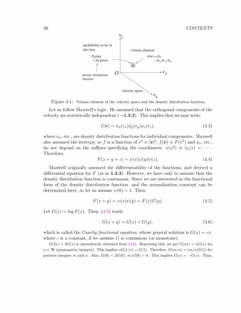
To make the kinetic theory quantitative, we must know the probability of a particleto assume various velocities. For the velocity to be v exactly is obviously probabilityzero. In our case Ω = v | vx, vy, vz ∈ R = R3. Thus, we need P defined on Ω. INthe present case, P (A) → 0 as volume of A → 0, so we may define the probabilitydensity; symbolically (see Fig. 4.1),
f(v) =P (dτ(v))
dτ(v), (4.1)
where dτ is the volume element, which may be written as d3v = dvxdvydvz. Wehave
P (A) =
∫A
d3v f(v). (4.2)
(1d case is explained in detail in the lecture notes. →1.3.2, 1.3.3)
In his “Illustrations of the dynamical theory of gases” (1860) Maxwell introducedthe density distribution function f(v) of the velocity of gas particles.
36 CONTENTS
v
v
vx
y
z
v
dτ( ) = v d v3
= dddvx vy vz
volume element
P( d )τ( )v
probability to be in
this box
= f(v) τ( )d v
velocity space
Odensity distribution
function
Figure 4.1: Volume element of the velocity space and the density distribution function
Let us follow Maxwell’s logic. He assumed that the orthogonal components of thevelocity are statistically independent (→1.3.3). This implies that we may write
f(v) = φx(vx)φy(vy)φz(vz), (4.3)
where φx, etc., are density distribution functions for individual components. Maxwellalso assumed the isotropy, so f is a function of v2 ≡ |v|2, f(v) ≡ F (v2) and φx, etc.,do not depend on the suffixes specifying the coordinates: ψ(s2) ≡ φx(s) = · · · .Therefore,
F (x+ y + z) = ψ(x)ψ(y)ψ(z). (4.4)
Maxwell originally assumed the differentiability of the functions, and derived adifferential equation for F (as in 1.3.3). However, we have only to assume that thedensity distribution function is continuous. Since we are interested in the functionalform of the density distribution function, and the normalization constant can bedetermined later, so let us assume ψ(0) = 1. Then,
F (x+ y) = ψ(x)ψ(y) = F (x)F (y). (4.5)
Let G(x) = logF (x). Then, (4.5) reads
G(x+ y) = G(x) +G(y), (4.6)
which is called the Cauchy functional equation, whose general solution is G(x) = cx,where c is a constant, if we assume G is continuous (or monotone).
G(2x) = 2G(x) is immediately obtained from (4.6). Repeating this, we get G(nx) = nG(x) forn ∈N (nonnegative integers). This implies nG(1/n) = G(1). Therefore, G(m/n) = (m/n)G(1) forpositive integers m and n. Also, G(0) = 2G(0), so G(0) = 0. This implies G(x) = −G(x). Thus,
4. LECTURE 4: MAXWELL’S DISTRIBUTION 37
we have demonstrated that for q ∈ Q (rational numbers) G(q) = cq, where c = G(1) is a constant.Since we assume G to be continuous, G(x) = cx must hold for any real x.
This implies F (x) ∝ ecx; remember that normalization constant must be deter-mined. That is, we may write with a new constant c (> 0)
f(v) ∝ e−cv2
. (4.7)
Maxwell actually did not like the above derivation that assumes statistical inde-pendence of three orthogonal directions, and rederived it later.
We must compute the normalization constant and c. An easy way (the easiestway?) to compute the normalization constant is the following elegant method. Sincethe integral is positive, let us compute the square of what we want:[∫ ∞
−∞dx e−x2/2σ2
]2
=
∫ ∞
−∞dx e−x2/2σ2
∫ ∞
−∞dy e−y2/2σ2
=
∫R2
dxdy e−(x2+y2)/2σ2
.
(4.8)Now, we go to the polar coordinates (x, y)→ (r, θ):∫
R2dxdy e−(x2+y2)/2σ2
= 2π
∫ ∞
0
e−r2/2σ2
rdr = 2π
∫ ∞
0
dz e−z/σ2
= 2πσ2. (4.9)
Hence, ∫ ∞
−∞dx e−x2/2σ2
=√
2πσ. (4.10)
The Gaussian density distribution function g(x) generally has the following form:
g(x) =1√2πσ
e−(x−m)2/2σ2
, (4.11)
where E(x) = m and V (x) = σ2. Thus, we can know a Gaussian (density) distribu-tion function, if we know the expectation value and the variance.37.
Since 〈vx〉 = 0 and V (vx) = (2/m)(kBT/2) = kBT/m (the equipartition of kineticenergy), we have
φ(vx) =
√m
2πkBTe−mv2
x/2kBT , (4.12)
37We will discuss the general multivariate Gaussian distribution in Chapter 4. In this case we willknow that if we know the expectation value and the covariance matrix, we can fix the distribution.
38 CONTENTS
and
f(v) =
(m
2πkBT
)3/2
e−mv2/2kBT . (4.13)
This is Maxwell’s distribution function.
At this juncture, let us practice a basic trick. You must be able to compute the ex-pectation value of eαx, where α is generally a complex number. If α = −s (Res > 0,positive real part), it is the Laplace transformation of the distribution function; ifα = ik where k is real, 〈eikx〉 is the Fourier transform of the density distribution,and is called the generating function.
〈eαx〉 =1√2πσ
∫ ∞
−∞dx eαx−(x−m)2/2σ2
(4.14)
The standard trick to compute this integral is to complete the square as follows:
αx− 1
2σ2(x−m)2 = α(x−m)+αm− 1
2σ2(x−m)2 = − 1
2σ2(x−m−σ2α)2+
σ2α2
2+αm.
(4.15)Therefore, (4.14) can be rewritten as
〈eαx〉 =1√2πσ
∫ ∞
−∞dx e−(x−m−σ2α)2/2σ2+σ2α2/2 +αm. (4.16)
We shift the integration range by m + σ2α (or you can introduce a new integrationvariable x′ = x−m−σ2α). Then, the integration just gives the normalization factor,so
〈eαx〉 = eσ2α2/2 +αm. (4.17)
Notice thatd
dα〈eαx〉
∣∣∣∣α=0
= E(x) = m, (4.18)
andd2
dα2〈eα(x−m)〉
∣∣∣∣α=0
= V (x) = σ2. (4.19)
These formulas are generally true (the distribution need not be Gaussian) as you cansee from its derivation.
Let us review Bernoulli’s kinetic interpretation of pressure. The (kinetic interpre-tation of) pressure on the wall is the average momentum (impulse) given to the wall
4. LECTURE 4: MAXWELL’S DISTRIBUTION 39
per unit time and area. Consider the wall perpendicular to the x-axis. Then, thenumber of particles with its x-component of the velocity being vx that can impingeon the unit area on the wall per unit time is given by nvx
∫dvy
∫dvzf(v),38 where n
is the number density of the gas molecules. Each particle gives the momentum 2mvx
upon collision to the wall, so
P =
∫vx≥0
dv 2mnv2xf(v) =
∫dvmnv2
xf(v) =1
3mn〈v2〉, (4.20)
where we have used the symmetry f(v) = f(−v), and the isotropy, 〈v2x〉 = 〈v2
y〉 =〈v2
x〉 = (1/3)〈v2x + v2
y + v2x〉. Or,
PV =2
3N〈K〉, (4.21)
where K is the kinetic energy of the single gas particle, and N is the number ofparticles in the volume V . This equation is called Bernoulli’s equation.
Comparing this with the equation of state of an ideal gas PV = NkBT , we obtainthe well-known relation:
〈v2〉 = 3kBT/m. (4.22)
Remark. Although the Boyle-Charles law is obtained, this does not tell us anythingabout molecules, because we do not know N . We cannot tell the mass of the particle,either. Remember that kB was not known when the kinetic theory of gases was beingdeveloped.
A notable point is that with empirical results that can be obtained from strictlyequilibrium studies, we cannot tell anything about molecules. Remember that thelaw of combined volume (→1.1.7) for chemical reactions crucial to demonstratethe particular nature of chemical substances are about (often violent) irreversibleprocesses from the reactants to the products. ut
Again, let us derive Maxwell’s distribution in a more elementary fashion, followingFeynman (again). Consider the force balance on the slice between heights h and h+dhof a cylinder with cross-section A. If n is the number density and m the mass of themolecules, we have as a force balance equation with the aid of P = nkBT
Anmgdh = −AdP = −AkBTdn (4.23)
38Precisely speaking, we must speak about the number of particles in the (velocity) volumeelement d3v, that is, nvxf(v)d3v, but throughout these notes, such obvious details may be omitted.
40 CONTENTS
ordn
dh= −βnmg. (4.24)
That is,39
n = n0e−βmgh. (4.25)
This can describe the sedimentation equilibrium of colloidal particles. More generally,the same logic derives for conserved forces with potential U
n(r) = n(0)e−β[U(r)−U(0)]. (4.26)
That is, the factor e−βU called the Boltzmann factor tells us the ratio of particledensities (or the probabilities to find particles) at different locations, when there isa position dependent potential energy U .
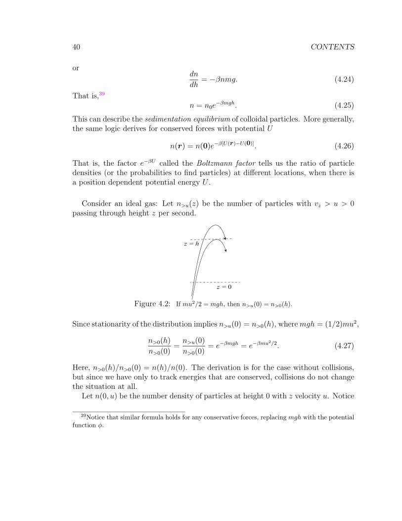
Consider an ideal gas: Let n>u(z) be the number of particles with vz > u > 0passing through height z per second.
z = h
z = 0
Figure 4.2: If mu2/2 = mgh, then n>u(0) = n>0(h).
Since stationarity of the distribution implies n>u(0) = n>0(h), wheremgh = (1/2)mu2,
n>0(h)
n>0(0)=n>u(0)
n>0(0)= e−βmgh = e−βmu2/2. (4.27)
Here, n>0(h)/n>0(0) = n(h)/n(0). The derivation is for the case without collisions,but since we have only to track energies that are conserved, collisions do not changethe situation at all.
Let n(0, u) be the number density of particles at height 0 with z velocity u. Notice
39Notice that similar formula holds for any conservative forces, replacing mgh with the potentialfunction φ.
4. LECTURE 4: MAXWELL’S DISTRIBUTION 41
that faster particles pass height 0 more than slower ones, so we must take care of thespeed in the z-direction:
n>u(0) =
∫ ∞
u
un(0, u) du ∝ e−βmu2/2. (4.28)
Thus, n(0, u) ∝ e−βmu2/2.
At the end of the 1857 paper Clausius calculated the speed of molecules at 0C:oxygen 461m/s, nitrogen 492m/s, and hydrogen 1,844m/s (the same order as thesound speed). Dutch meteorologist C. H. D. Buys-Ballot (1817-1890)40 noticed thatif the molecules of gases really moved that fast, the mixing of gases by diffusionshould have been much faster than we observed it to be.
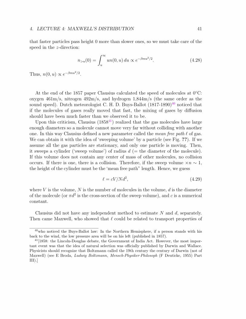
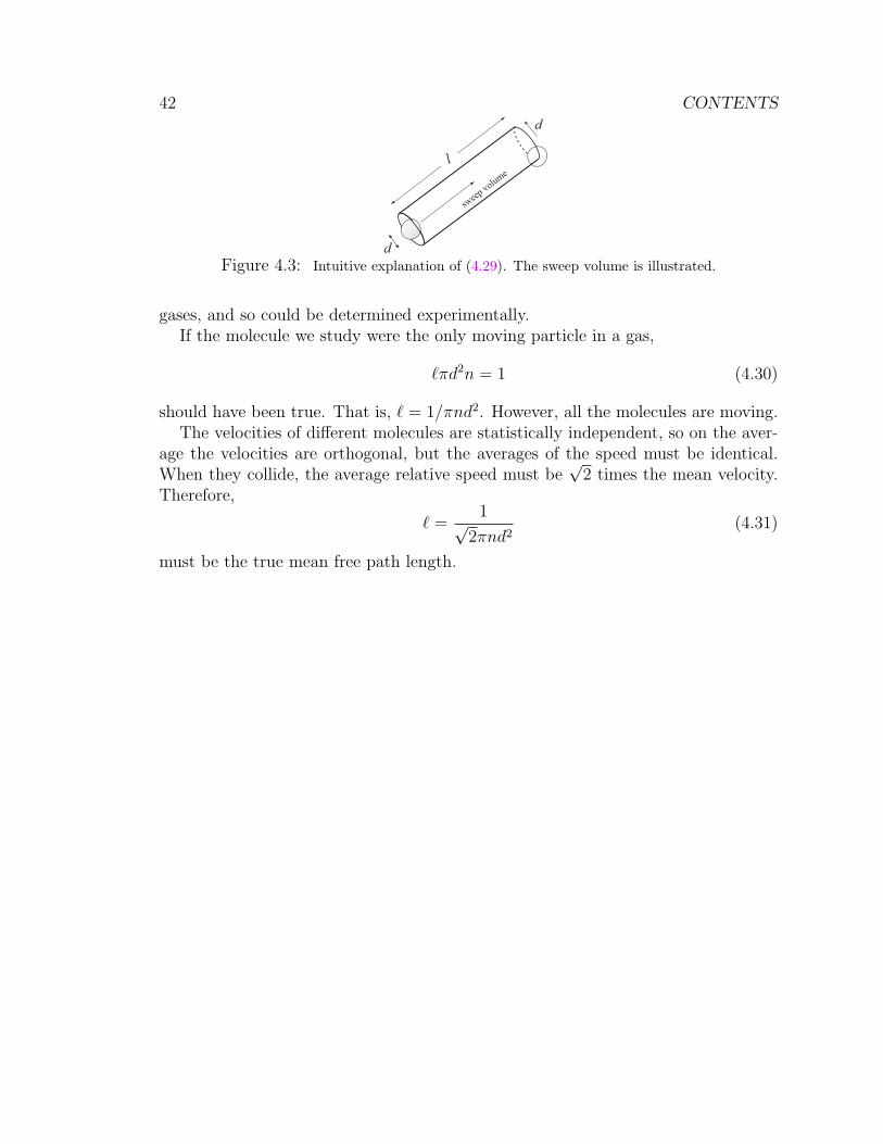
Upon this criticism, Clausius (185841) realized that the gas molecules have largeenough diameters so a molecule cannot move very far without colliding with anotherone. In this way Clausius defined a new parameter called the mean free path ` of gas.We can obtain it with the idea of ‘sweeping volume’ by a particle (see Fig. ??). If weassume all the gas particles are stationary, and only one particle is moving. Then,it sweeps a cylinder (‘sweep volume’) of radius d (= the diameter of the molecule).If this volume does not contain any center of mass of other molecules, no collisionoccurs. If there is one, there is a collision. Therefore, if the sweep volume ×n ∼ 1,the height of the cylinder must be the ‘mean free path” length. Hence, we guess
` = cV/Nd2, (4.29)
where V is the volume, N is the number of molecules in the volume, d is the diameterof the molecule (or πd2 is the cross-section of the sweep volume), and c is a numericalconstant.
Clausius did not have any independent method to estimate N and d, separately.Then came Maxwell, who showed that ` could be related to transport properties of
40who noticed the Buys-Ballot law: In the Northern Hemisphere, if a person stands with hisback to the wind, the low pressure area will be on his left (published in 1857).
41[1858: the Lincoln-Douglas debate, the Government of India Act. However, the most impor-tant event was that the idea of natural selection was officially published by Darwin and Wallace.Physicists should recognize that Boltzmann called the 19th century the century of Darwin (not ofMaxwell) (see E Broda, Ludwig Boltzmann, Mensch·Physiker·Philosoph (F Deuticke, 1955) PartIII).]
42 CONTENTS
d
l
d
swee
p volu
me
Figure 4.3: Intuitive explanation of (4.29). The sweep volume is illustrated.
gases, and so could be determined experimentally.If the molecule we study were the only moving particle in a gas,
`πd2n = 1 (4.30)
should have been true. That is, ` = 1/πnd2. However, all the molecules are moving.The velocities of different molecules are statistically independent, so on the aver-
age the velocities are orthogonal, but the averages of the speed must be identical.When they collide, the average relative speed must be
√2 times the mean velocity.
Therefore,
` =1√
2πnd2(4.31)
must be the true mean free path length.
5. LECTURE 5: SIMPLE KINETIC THEORY OF TRANSPORT PHENOMENA43
5 Lecture 5: Simple kinetic theory of transport
phenomena
Summary∗ Transport phenomena are outlined. Fluxes are proportional to (−)gradients of the
density fields.∗ Transport coefficients can be estimated with the aid of elementary kinetic theory.∗ Maxwell used shear viscosity and the van der Waals equation of state to estimate
Avogadro’s constant and the molecular size for the first time.∗ If a mesoscopic object is placed in a gas, due to molecular bombardment, it jiggles
and wanders around = Brownian motion. Its displacement distance ∆ duringtime t is roughly ∆ ∝
√t.
∗ Langevin explained this behavior, starting from the Newton’s equation of motionwith a stochastic driving force.
∗ The trajectory of a Brownian particle after coarse-grained may be understood asa random walk, which is closely relate to the polymer conformation.
Key wordsTransport phenomena, flux, gradient, transport coefficient, shear viscosity, diffusion,Brownian motion, Langevin equation, random walk, random polymer
What you should be able to do∗ Understand how to handle the averages of vector components.∗ You should be able to follow Langevin’s logic and calculation.∗ Be able to demonstrate that a random walker after n unit steps is about
√n from
her starting point.
The derivation of the mean free path length
` =1√
2πnd2(5.1)
may not have been convincing. ` must be the mean traveling distance in t/averagenumber of collisions in t. The mean traveling distance in t may be represented by theroot-mean square velocity v times t. The collision occurs with the relative velocity
44 CONTENTS
w. Therefore, z = wπd2nt must be the total number of collisions (we follow the ideaof the sweep volume again). Hence,
` =vt
wπd2nt=
1√2πd2n
. (5.2)
This was the formula we guessed.
Maxwell used the idea of mean free path to compute the shear viscosity. Beforegoing to this calculation we discuss the general transport phenomena.
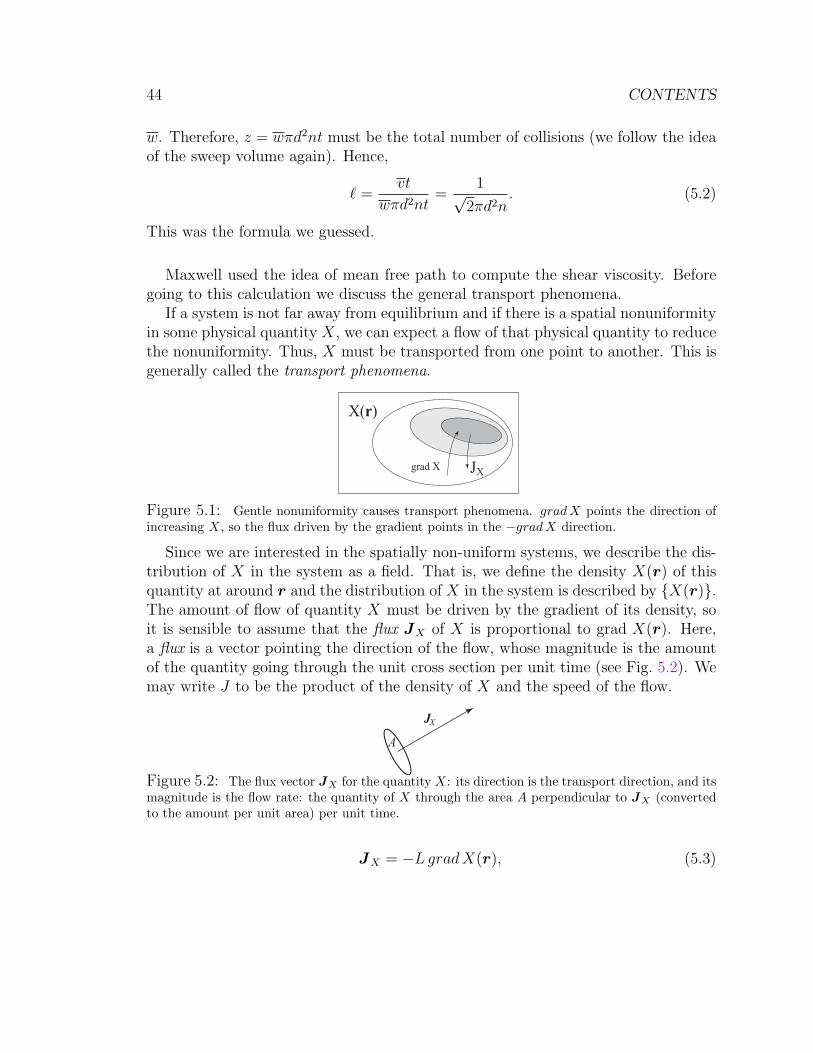
If a system is not far away from equilibrium and if there is a spatial nonuniformityin some physical quantity X, we can expect a flow of that physical quantity to reducethe nonuniformity. Thus, X must be transported from one point to another. This isgenerally called the transport phenomena.
grad X
X(r)
JX
Figure 5.1: Gentle nonuniformity causes transport phenomena. grad X points the direction ofincreasing X, so the flux driven by the gradient points in the −grad X direction.
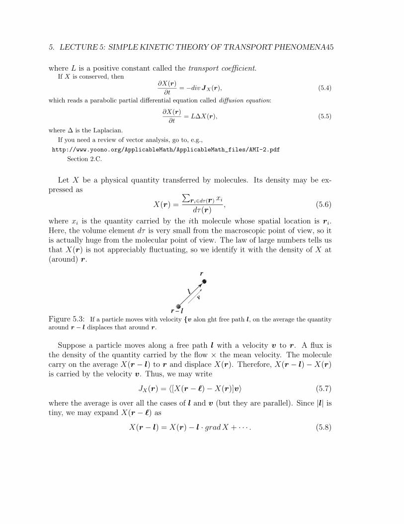
Since we are interested in the spatially non-uniform systems, we describe the dis-tribution of X in the system as a field. That is, we define the density X(r) of thisquantity at around r and the distribution of X in the system is described by X(r).The amount of flow of quantity X must be driven by the gradient of its density, soit is sensible to assume that the flux JX of X is proportional to grad X(r). Here,a flux is a vector pointing the direction of the flow, whose magnitude is the amountof the quantity going through the unit cross section per unit time (see Fig. 5.2). Wemay write J to be the product of the density of X and the speed of the flow.
J
A
X
Figure 5.2: The flux vector JX for the quantity X: its direction is the transport direction, and itsmagnitude is the flow rate: the quantity of X through the area A perpendicular to JX (convertedto the amount per unit area) per unit time.
JX = −LgradX(r), (5.3)
5. LECTURE 5: SIMPLE KINETIC THEORY OF TRANSPORT PHENOMENA45
where L is a positive constant called the transport coefficient.If X is conserved, then
∂X(r)∂t
= −div JX(r), (5.4)
which reads a parabolic partial differential equation called diffusion equation:
∂X(r)∂t
= L∆X(r), (5.5)
where ∆ is the Laplacian.If you need a review of vector analysis, go to, e.g.,
http://www.yoono.org/ApplicableMath/ApplicableMath_files/AMI-2.pdf
Section 2.C.
Let X be a physical quantity transferred by molecules. Its density may be ex-pressed as
X(r) =
∑ri∈dτ(r) xi
dτ(r), (5.6)
where xi is the quantity carried by the ith molecule whose spatial location is ri.Here, the volume element dτ is very small from the macroscopic point of view, so itis actually huge from the molecular point of view. The law of large numbers tells usthat X(r) is not appreciably fluctuating, so we identify it with the density of X at(around) r.
l
v
r
−r
l
Figure 5.3: If a particle moves with velocity v alon ght free path l, on the average the quantityaround r − l displaces that around r.
Suppose a particle moves along a free path l with a velocity v to r. A flux isthe density of the quantity carried by the flow × the mean velocity. The moleculecarry on the average X(r − l) to r and displace X(r). Therefore, X(r − l)−X(r)is carried by the velocity v. Thus, we may write
JX(r) = 〈[X(r − `)−X(r)]v〉 (5.7)
where the average is over all the cases of l and v (but they are parallel). Since |l| istiny, we may expand X(r − `) as
X(r − l) = X(r)− l · gradX + · · · . (5.8)
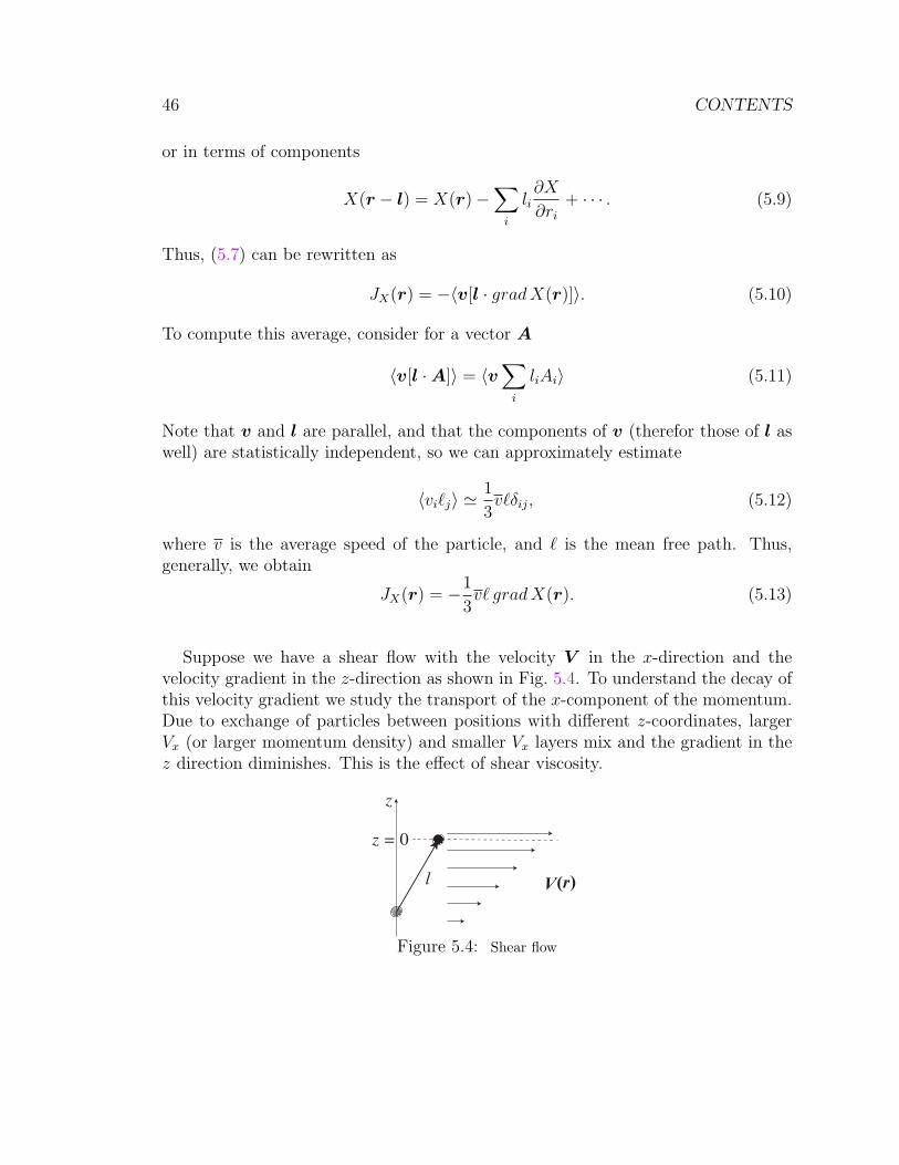
46 CONTENTS
or in terms of components
X(r − l) = X(r)−∑
i
li∂X
∂ri
+ · · · . (5.9)
Thus, (5.7) can be rewritten as
JX(r) = −〈v[l · gradX(r)]〉. (5.10)
To compute this average, consider for a vector A
〈v[l ·A]〉 = 〈v∑
i
liAi〉 (5.11)
Note that v and l are parallel, and that the components of v (therefor those of l aswell) are statistically independent, so we can approximately estimate
〈vi`j〉 '1
3v`δij, (5.12)
where v is the average speed of the particle, and ` is the mean free path. Thus,generally, we obtain
JX(r) = −1
3v` gradX(r). (5.13)
Suppose we have a shear flow with the velocity V in the x-direction and thevelocity gradient in the z-direction as shown in Fig. 5.4. To understand the decay ofthis velocity gradient we study the transport of the x-component of the momentum.Due to exchange of particles between positions with different z-coordinates, largerVx (or larger momentum density) and smaller Vx layers mix and the gradient in thez direction diminishes. This is the effect of shear viscosity.
V r( )l
z = 0
z
Figure 5.4: Shear flow
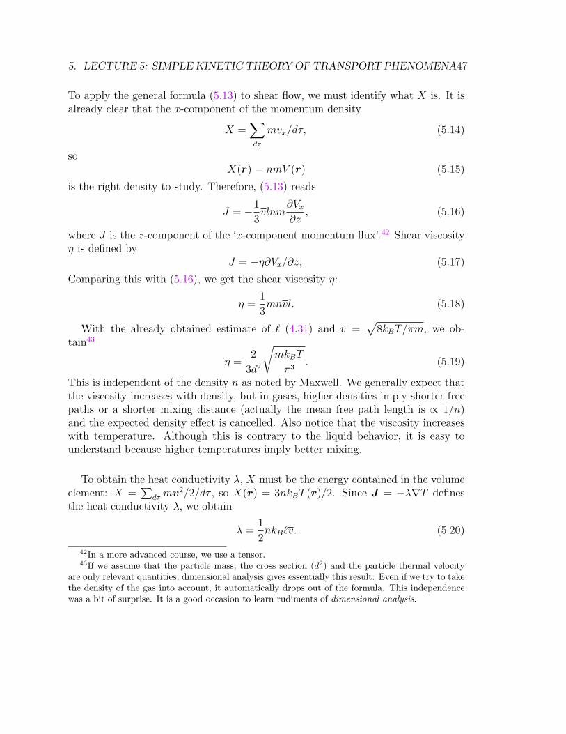
5. LECTURE 5: SIMPLE KINETIC THEORY OF TRANSPORT PHENOMENA47
To apply the general formula (5.13) to shear flow, we must identify what X is. It isalready clear that the x-component of the momentum density
X =∑dτ
mvx/dτ, (5.14)
soX(r) = nmV (r) (5.15)
is the right density to study. Therefore, (5.13) reads
J = −1
3vlnm
∂Vx
∂z, (5.16)
where J is the z-component of the ‘x-component momentum flux’.42 Shear viscosityη is defined by
J = −η∂Vx/∂z, (5.17)
Comparing this with (5.16), we get the shear viscosity η:
η =1
3mnvl. (5.18)
With the already obtained estimate of ` (4.31) and v =√
8kBT/πm, we ob-tain43
η =2
3d2
√mkBT
π3. (5.19)
This is independent of the density n as noted by Maxwell. We generally expect thatthe viscosity increases with density, but in gases, higher densities imply shorter freepaths or a shorter mixing distance (actually the mean free path length is ∝ 1/n)and the expected density effect is cancelled. Also notice that the viscosity increaseswith temperature. Although this is contrary to the liquid behavior, it is easy tounderstand because higher temperatures imply better mixing.
To obtain the heat conductivity λ, X must be the energy contained in the volumeelement: X =
∑dτ mv2/2/dτ , so X(r) = 3nkBT (r)/2. Since J = −λ∇T defines
the heat conductivity λ, we obtain
λ =1
2nkB`v. (5.20)
42In a more advanced course, we use a tensor.43If we assume that the particle mass, the cross section (d2) and the particle thermal velocity
are only relevant quantities, dimensional analysis gives essentially this result. Even if we try to takethe density of the gas into account, it automatically drops out of the formula. This independencewas a bit of surprise. It is a good occasion to learn rudiments of dimensional analysis.
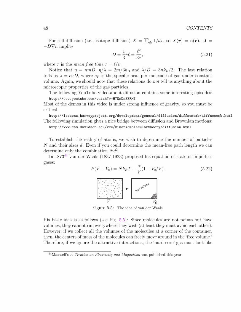
48 CONTENTS
For self-diffusion (i.e., isotope diffusion) X =∑
dτ 1/dτ , so X(r) = n(r). J =−D∇n implies
D =1
3v` =
`2
3τ, (5.21)
where τ is the mean free time τ = `/v.Notice that η = nmD, η/λ = 2m/3kB and λ/D = 3nkB/2. The last relation
tells us λ = cVD, where cV is the specific heat per molecule of gas under constantvolume. Again, we should note that these relations do not tell us anything about themicroscopic properties of the gas particles.
The following YouTube video about diffusion contains some interesting episodes:http://www.youtube.com/watch?v=H7QsDs8ZRMI
Most of the demos in this video is under strong influence of gravity, so you must becritical.
http://lessons.harveyproject.org/development/general/diffusion/diffnomemb/diffnomemb.html
The following simulation gives a nice bridge between diffusion and Brownian motions:http://www.chm.davidson.edu/vce/kineticmoleculartheory/diffusion.html
To establish the reality of atoms, we wish to determine the number of particlesN and their sizes d. Even if you could determine the mean-free path length we candetermine only the combination Nd2.
In 187344 van der Waals (1837-1923) proposed his equation of state of imperfectgases:
P (V − V0) = NkBT −α
V(1− V0/V ). (5.22)
V V0
free v
olum
e
Figure 5.5: The idea of van der Waals.
His basic idea is as follows (see Fig. 5.5): Since molecules are not points but havevolumes, they cannot run everywhere they wish (at least they must avoid each other).However, if we collect all the volumes of the molecules at a corner of the container,then, the centers of mass of the molecules can freely move around in the ‘free volume.’Therefore, if we ignore the attractive interactions, the ‘hard-core’ gas must look like
44Maxwell’s A Treatise on Electricity and Magnetism was published this year.
5. LECTURE 5: SIMPLE KINETIC THEORY OF TRANSPORT PHENOMENA49
an ideal gas with a reduced volume:
P (V − V0) = NkBT. (5.23)
The remaining part of the van der Waals equation is to take care of the attractiveintermolecular forces. Thus, from V0 ' bNπd3/6, where b is a geometrical constantof order unity, we can estimate the size of the molecules. Now, we know Nd2 andNd3, so we can estimate N and d. The method gives an estimate of Avogadro’sconstant NA ' (4 ∼ 6)× 1023.45
Since molecules are incessantly moving around vigorously, small objects shouldnot be able to sit still in fluids even in equilibrium. Indeed, we know Brownianmotions. Let us watch some examples:
Nanoparticles in water:http://www.youtube.com/watch?v=cDcprgWiQEY&feature=topics
Simulationshttp://www.phy.ntnu.edu.tw/ntnujava/index.php?topic=24.msg158#msg158
http://www.youtube.com/watch?v=PtYP8uoN0lk&feature=topics
The Brownian motion was discovered in the summer of 1827.46,47 We are usuallygiven an impression that he simply observed the “Brownian motion.” However, hedid a very careful and thorough research to establish the universal nature of themotion.
Since the particles came from living cells, initially he thought that it was a vi-tal phenomenon. Removing the effect of advection, evaporation, etc., carefully, hetested many flowers. Then, he tested old pollens in the British Museum (he wasthe (founding) director of the Botanical Division), and still found active particles.He conjectured that this was an organic effect, testing even coal with no exceptionfound. This suggested him that not only vital but organic nature of the specimens
45〈〈Definition of Avogadro’s constant〉〉 This is defined as the number of atoms in a 0.012kg of 12C. The latest Avogadro constant value is due to B. Andreas et al., “Determination of theAvogadro constant by counting the atoms in a 28Si crystal,” Phys. Rev. Lett., 106, 030801 (2011).Cf. P. Beker, “History and progress in the accurate determination of the Avogadro constant,” RepProg Phys 64 1945 (2001).
46Beethoven died in March; Democratic party was founded.47The work was published the next year, but was communicated to Stokes very soon in August,
1827. See P Pearle, B Collett, K Bart, D Bilderback, D Newman, and S Samuels, “What Brownsaw and you can too,” Am. J. Phys. 78, 1278 (2010).

50 CONTENTS
were irrelevant. He then tested numerous inorganic specimens (including a piece ofSphinx; he also roasted his specimens).
Thus, he really deserves the name of the motion. As to Mr. Brown himself, see1.4.4.
Curiously enough, there was no work published on the Brownian motion between1831 and 1857, but the phenomenon was well known. From 1850s new experimentalstudies began by Gouy (1854-1926) and others. The established facts included (youwould find them very easy to understand in terms of molecular bombardment onmesoscopic particles):(1) Its trajectory is quite erratic without any tangent lines anywhere.(2) Two Brownian particles are statistically independent even when they come withintheir diameters.(3) Smaller particles move more vigorously.(4) The higher the temperature, the more vigorous the Brownian motion.(5) The smaller the viscosity of the fluid medium, the more vigorous the motion.(6) The motion never dies out.etc.
In the 1860s there were experimentalists who clearly recognized that the motionwas due to the impact of water molecules. Even Poincare (1854-1912) mentioned thismotion in 1900, but somehow no founding fathers of kinetic theory and statisticalmechanics paid any attention to Brownian motion.
Due to the bombardment of water molecules, the Brownian particle executes azigzag motion, and on the average it is displaced as seen in Fig. 5.6 (ref 1 =https://commons.wikimedia.org/wiki/File:500_frames_of_brownian_motion_integrated.ogv?uselang=de).
This site exhibits how the (Gaussian) distribution is accumulated.
As you see the salient feature of the Brownian displacement ∆x is
〈∆x2〉 ∝ t, (5.24)
where 〈 〉 is the ensemble average (you repeat the experiment again and again ordo many experiments simultaneously, and average the results) t is time, and theproportionality constant is related to (proportional to) the diffusion constant.
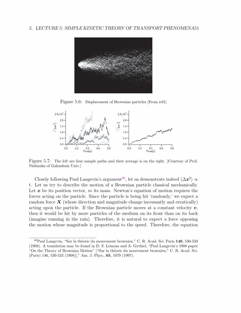
5. LECTURE 5: SIMPLE KINETIC THEORY OF TRANSPORT PHENOMENA51
Figure 5.6: Displacement of Brownian particles [From ref1]
Figure 5.7: The left are four sample paths and their average is on the right. [Courtesy of Prof.Nishizaka of Gakushuin Univ.]
Closely following Paul Langevin’s argument48, let us demonstrate indeed 〈∆x2〉 ∝t. Let us try to describe the motion of a Brownian particle classical mechanically.Let x be its position vector, m its mass. Newton’s equation of motion requires theforces acting on the particle. Since the particle is being hit ‘randomly,’ we expect arandom force X (whose direction and magnitude change incessantly and erratically)acting upon the particle. If the Brownian particle moves at a constant velocity v,then it would be hit by more particles of the medium on its front than on its back(imagine running in the rain). Therefore, it is natural to expect a force opposingthe motion whose magnitude is proportional to the speed. Therefore, the equation
48Paul Langevin, “Sur la theorie du mouvement brownien,” C. R. Acad. Sci. Paris 146, 530-533(1908). A translation may be found in D. S. Lemons and A. Gythiel, “Paul Langevin’s 1908 paper“On the Theory of Brownian Motion” [“Sur la theorie du mouvement brownien,” C. R. Acad. Sci.(Paris) 146, 530-533 (1908)],” Am. J. Phys., 65, 1079 (1997).
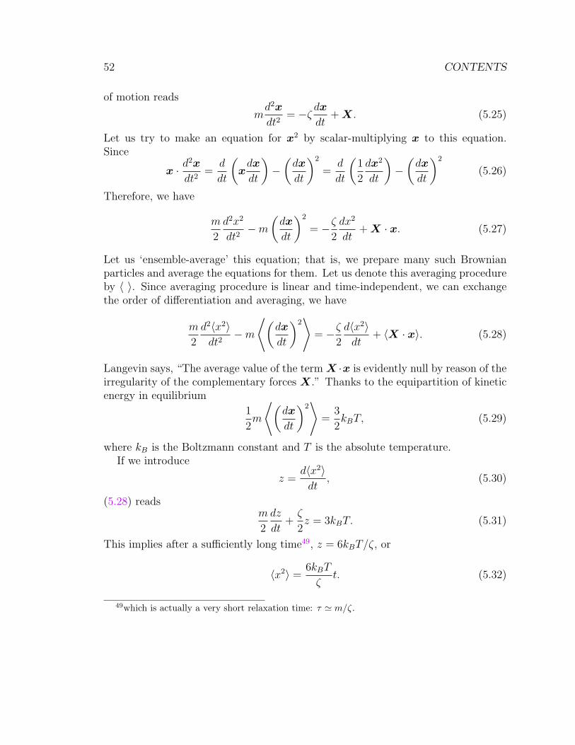
52 CONTENTS
of motion reads
md2x
dt2= −ζ dx
dt+ X. (5.25)
Let us try to make an equation for x2 by scalar-multiplying x to this equation.Since
x · d2x
dt2=
d
dt
(xdx
dt
)−(dx
dt
)2
=d
dt
(1
2
dx2
dt
)−(dx
dt
)2
(5.26)
Therefore, we have
m
2
d2x2
dt2−m
(dx
dt
)2
= −ζ2
dx2
dt+ X · x. (5.27)
Let us ‘ensemble-average’ this equation; that is, we prepare many such Brownianparticles and average the equations for them. Let us denote this averaging procedureby 〈 〉. Since averaging procedure is linear and time-independent, we can exchangethe order of differentiation and averaging, we have
m
2
d2〈x2〉dt2
−m
⟨(dx
dt
)2⟩
= −ζ2
d〈x2〉dt
+ 〈X · x〉. (5.28)
Langevin says, “The average value of the term X ·x is evidently null by reason of theirregularity of the complementary forces X.” Thanks to the equipartition of kineticenergy in equilibrium
1
2m
⟨(dx
dt
)2⟩
=3
2kBT, (5.29)
where kB is the Boltzmann constant and T is the absolute temperature.If we introduce
z =d〈x2〉dt
, (5.30)
(5.28) readsm
2
dz
dt+ζ
2z = 3kBT. (5.31)
This implies after a sufficiently long time49, z = 6kBT/ζ, or
〈x2〉 =6kBT
ζt. (5.32)
49which is actually a very short relaxation time: τ ' m/ζ.
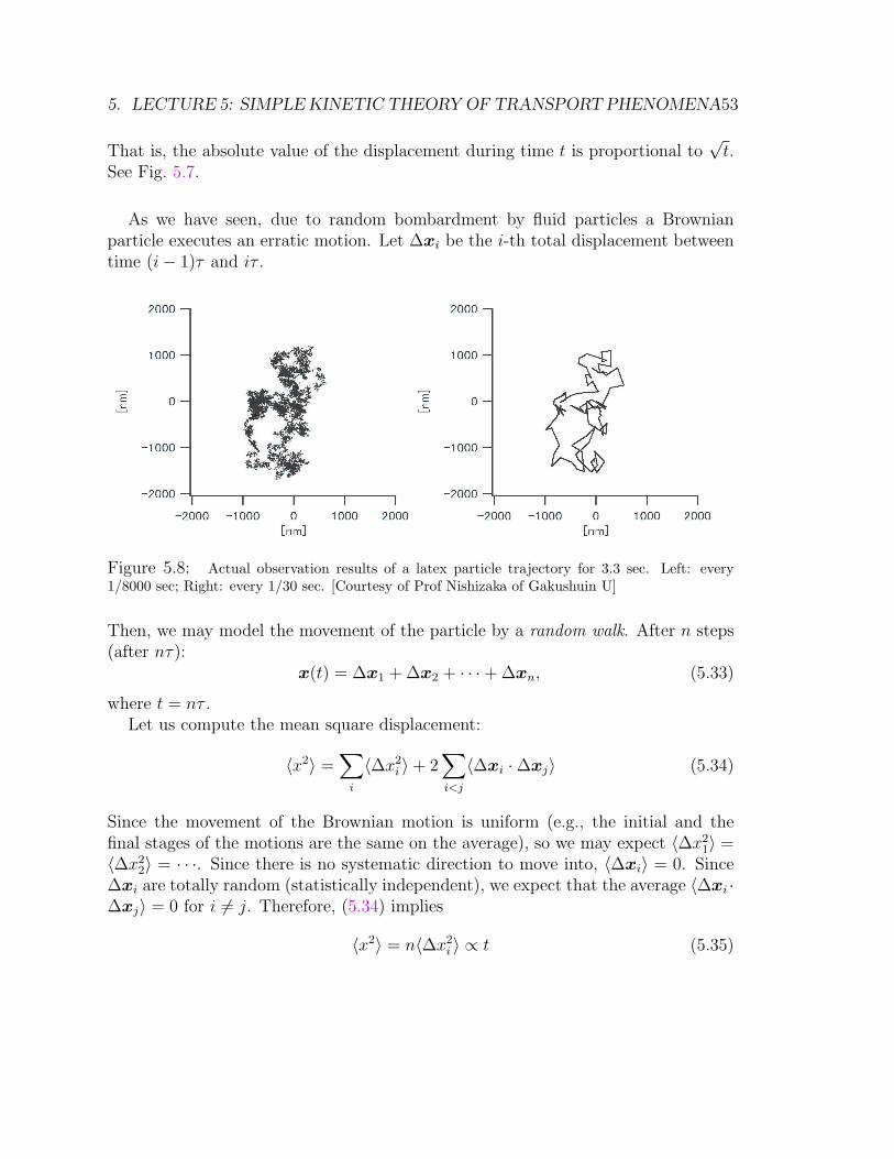
5. LECTURE 5: SIMPLE KINETIC THEORY OF TRANSPORT PHENOMENA53
That is, the absolute value of the displacement during time t is proportional to√t.
See Fig. 5.7.
As we have seen, due to random bombardment by fluid particles a Brownianparticle executes an erratic motion. Let ∆xi be the i-th total displacement betweentime (i− 1)τ and iτ .
Figure 5.8: Actual observation results of a latex particle trajectory for 3.3 sec. Left: every1/8000 sec; Right: every 1/30 sec. [Courtesy of Prof Nishizaka of Gakushuin U]
Then, we may model the movement of the particle by a random walk. After n steps(after nτ):
x(t) = ∆x1 + ∆x2 + · · ·+ ∆xn, (5.33)
where t = nτ .Let us compute the mean square displacement:
〈x2〉 =∑
i
〈∆x2i 〉+ 2
∑i<j
〈∆xi ·∆xj〉 (5.34)
Since the movement of the Brownian motion is uniform (e.g., the initial and thefinal stages of the motions are the same on the average), so we may expect 〈∆x2
1〉 =〈∆x2
2〉 = · · ·. Since there is no systematic direction to move into, 〈∆xi〉 = 0. Since∆xi are totally random (statistically independent), we expect that the average 〈∆xi ·∆xj〉 = 0 for i 6= j. Therefore, (5.34) implies
〈x2〉 = n〈∆x2i 〉 ∝ t (5.35)
54 CONTENTS
This is consistent with (5.32).
We can consider a random walk on a lattice. Let `i be the ith step of the walk.Starting from the origin, a random walk of n steps on a lattice may be definedas
R(n) = `1 + `2 + · · ·+ `n, (5.36)
where `i are chosen from the bond vectors, and R(n) is the position of the walk aftern steps. If the lattice spacing is unity, then the consideration in ?? tells us
〈R(n)2〉 = n. (5.37)
We may interpret the trajectory of a random walk as a conformation of a polymerconsisting of n monomers (without any steric interactions among monomer units ex-cept perhaps for bond angle constraints). Then, R(n) is the end-to-end vector of thepolymer chain, and the root-mean square end-to-end distance satisfies (5.37).
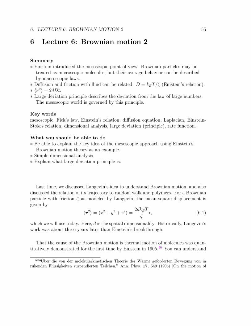
6. LECTURE 6: BROWNIAN MOTION 2 55
6 Lecture 6: Brownian motion 2
Summary∗ Einstein introduced the mesoscopic point of view: Brownian particles may be
treated as microscopic molecules, but their average behavior can be describedby macroscopic laws.
∗ Diffusion and friction with fluid can be related: D = kBT/ζ (Einstein’s relation).∗ 〈r2〉 = 2dDt.∗ Large deviation principle describes the deviation from the law of large numbers.
The mesoscopic world is governed by this principle.
Key wordsmesoscopic, Fick’s law, Einstein’s relation, diffusion equation, Laplacian, Einstein-Stokes relation, dimensional analysis, large deviation (principle), rate function.
What you should be able to do∗ Be able to explain the key idea of the mesoscopic approach using Einstein’s
Brownian motion theory as an example.∗ Simple dimensional analysis.∗ Explain what large deviation principle is.
Last time, we discussed Langevin’s idea to understand Brownian motion, and alsodiscussed the relation of its trajectory to random walk and polymers. For a Brownianparticle with friction ζ as modeled by Langevin, the mean-square displacement isgiven by
〈r2〉 = 〈x2 + y2 + z2〉 =2dkBT
ζt, (6.1)
which we will use today. Here, d is the spatial dimensionality. Historically, Langevin’swork was about three years later than Einstein’s breakthrough.
That the cause of the Brownian motion is thermal motion of molecules was quan-titatively demonstrated for the first time by Einstein in 1905.50 You can understand
50“Uber die von der molekularkinetischen Theorie der Warme geforderten Bewegung von inruhenden Flussigkeiten suspendierten Teilchen,” Ann. Phys. 17, 549 (1905) [On the motion of
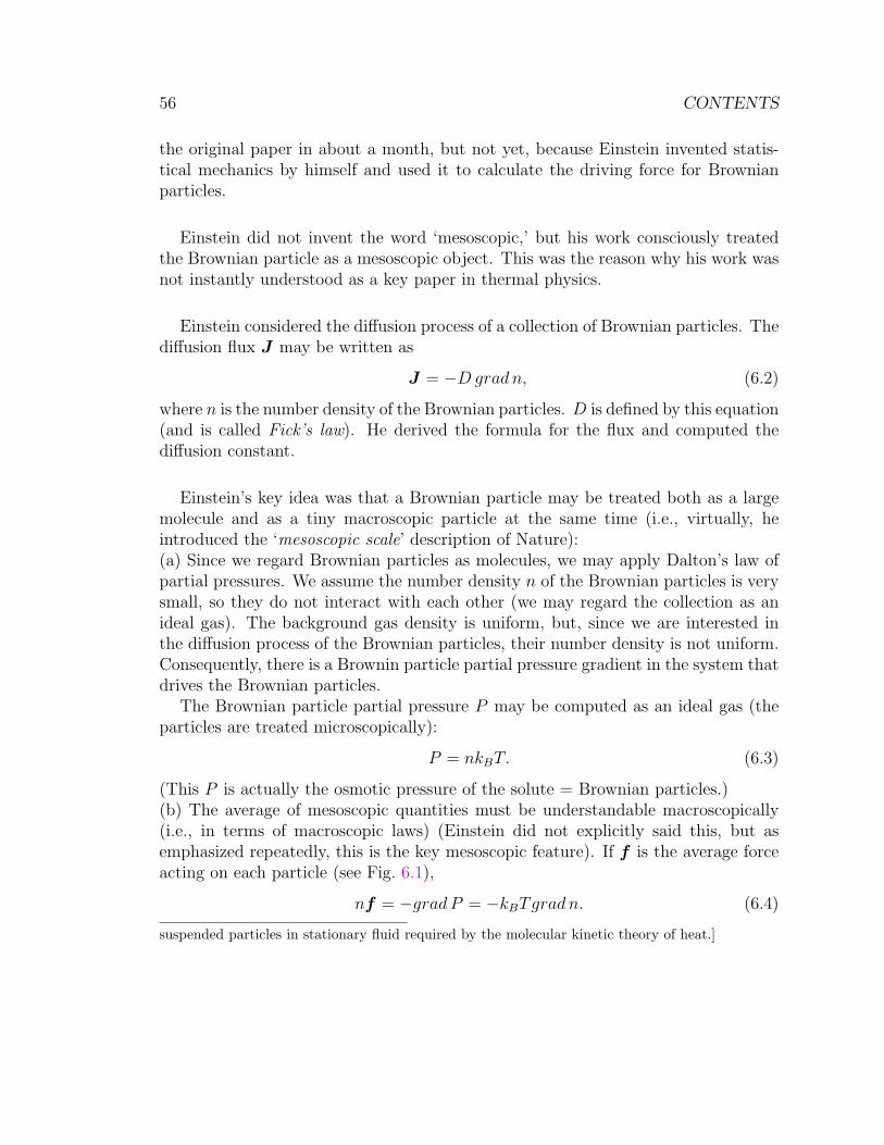
56 CONTENTS
the original paper in about a month, but not yet, because Einstein invented statis-tical mechanics by himself and used it to calculate the driving force for Brownianparticles.
Einstein did not invent the word ‘mesoscopic,’ but his work consciously treatedthe Brownian particle as a mesoscopic object. This was the reason why his work wasnot instantly understood as a key paper in thermal physics.
Einstein considered the diffusion process of a collection of Brownian particles. Thediffusion flux J may be written as
J = −D grad n, (6.2)
where n is the number density of the Brownian particles. D is defined by this equation(and is called Fick’s law). He derived the formula for the flux and computed thediffusion constant.
Einstein’s key idea was that a Brownian particle may be treated both as a largemolecule and as a tiny macroscopic particle at the same time (i.e., virtually, heintroduced the ‘mesoscopic scale’ description of Nature):(a) Since we regard Brownian particles as molecules, we may apply Dalton’s law ofpartial pressures. We assume the number density n of the Brownian particles is verysmall, so they do not interact with each other (we may regard the collection as anideal gas). The background gas density is uniform, but, since we are interested inthe diffusion process of the Brownian particles, their number density is not uniform.Consequently, there is a Brownin particle partial pressure gradient in the system thatdrives the Brownian particles.
The Brownian particle partial pressure P may be computed as an ideal gas (theparticles are treated microscopically):
P = nkBT. (6.3)
(This P is actually the osmotic pressure of the solute = Brownian particles.)(b) The average of mesoscopic quantities must be understandable macroscopically(i.e., in terms of macroscopic laws) (Einstein did not explicitly said this, but asemphasized repeatedly, this is the key mesoscopic feature). If f is the average forceacting on each particle (see Fig. 6.1),
nf = −gradP = −kBTgrad n. (6.4)
suspended particles in stationary fluid required by the molecular kinetic theory of heat.]
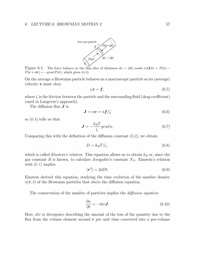
6. LECTURE 6: BROWNIAN MOTION 2 57
P(r)
P(r+dr)f
A
dx = |dr|
force per particle
Figure 6.1: The force balance at the thin slice of thickness dx = |dr| reads nAfdx = P (r) −P (r + dr) = −grad P (r), which gives (6.4).
On the average a Brownian particle behaves as a macroscopic particle so its (average)velocity v must obey
ζv = f , (6.5)
where ζ is the friction between the particle and the surrounding fluid (drag coefficient)(used in Langevin’s approach).
The diffusion flux J is
J = nv = nf/ζ (6.6)
so (6.4) tells us that
J = −kBT
ζgrad n. (6.7)
Comparing this with the definition of the diffusion constant (6.2), we obtain
D = kBT/ζ, (6.8)
which is called Einstein’s relation. This equation allows us to obtain kB or, since thegas constant R is known, to calculate Avogadro’s constant NA. Einstein’s relationwith (6.1) implies
〈r2〉 = 2dDt. (6.9)
Einstein derived this equation, studying the time evolution of the number densityn(r, t) of the Brownian particles that obeys the diffusion equation.
The conservation of the number of particles implies the diffusion equation:
∂n
∂t= −divJ . (6.10)
Here, div is divergence describing the amount of the loss of the quantity due to theflux from the volume element around r per unit time converted into a per-volume
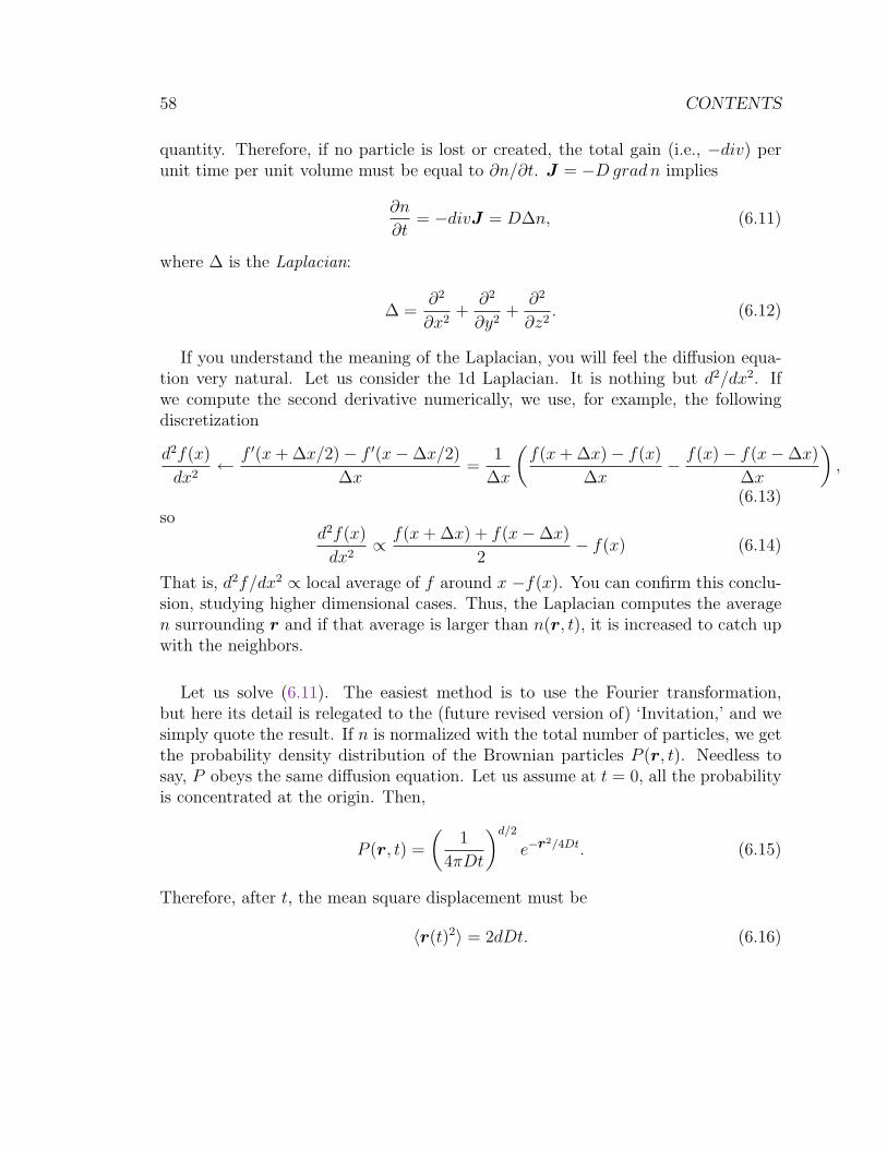
58 CONTENTS
quantity. Therefore, if no particle is lost or created, the total gain (i.e., −div) perunit time per unit volume must be equal to ∂n/∂t. J = −D grad n implies
∂n
∂t= −divJ = D∆n, (6.11)
where ∆ is the Laplacian:
∆ =∂2
∂x2+
∂2
∂y2+
∂2
∂z2. (6.12)
If you understand the meaning of the Laplacian, you will feel the diffusion equa-tion very natural. Let us consider the 1d Laplacian. It is nothing but d2/dx2. Ifwe compute the second derivative numerically, we use, for example, the followingdiscretization
d2f(x)
dx2← f ′(x+ ∆x/2)− f ′(x−∆x/2)
∆x=
1
∆x
(f(x+ ∆x)− f(x)
∆x− f(x)− f(x−∆x)
∆x
),
(6.13)so
d2f(x)
dx2∝ f(x+ ∆x) + f(x−∆x)
2− f(x) (6.14)
That is, d2f/dx2 ∝ local average of f around x −f(x). You can confirm this conclu-sion, studying higher dimensional cases. Thus, the Laplacian computes the averagen surrounding r and if that average is larger than n(r, t), it is increased to catch upwith the neighbors.
Let us solve (6.11). The easiest method is to use the Fourier transformation,but here its detail is relegated to the (future revised version of) ‘Invitation,’ and wesimply quote the result. If n is normalized with the total number of particles, we getthe probability density distribution of the Brownian particles P (r, t). Needless tosay, P obeys the same diffusion equation. Let us assume at t = 0, all the probabilityis concentrated at the origin. Then,
P (r, t) =
(1
4πDt
)d/2
e−r2/4Dt. (6.15)
Therefore, after t, the mean square displacement must be
〈r(t)2〉 = 2dDt. (6.16)
6. LECTURE 6: BROWNIAN MOTION 2 59
That is, if we observe the mean square displacement of a particle, then the diffusionconstant D of the collection of such particles may be measured.
Let us summarize Einstein’s fundamental idea, which is the key idea of nonequi-librium statistical mechanics as we will learn later:
Microscopic fluctuations can build up (semi)macroscopic fluctuations whosedynamics is on the average governed by the laws of macroscopic time evo-lution.
Brownian motion is a semimacroscopic (mesoscopic) motion that is a result of build-ing up of microscopic fluctuations. Its decay is described by a macroscopic dissipativedynamics.
This was later more clearly stated by Onsager as the regression hypothesis.
Einstein’s original paper use ζ = 6πaη, where a is the radius of the Brownianparticle, and η is the shear viscosity of the fluid. Thus, the original Einstein’s relationreads
D =kBT
6πaη. (6.17)
Here, Stokes’ law is used that gives the drag force acting on a sphere of radius amoving at velocity v relative to the surrounding fluid: f = 6πaηv.51
D ∝ kBT/aη is concluded with the aid of dimensional analysis. Since dimensionalanalysis is quite important, let us derive this relation dimensional-analytically.
An introduction to dimensional analysis is available:http://www.yoono.org/Y_OONO_official_site/download_files/DAmemo_1.pdf.The dimension of a quantity X is usually denoted by [X]. The basic dimensions arelength L, mass M and time T . For example, [a] = L. If you know the unit of aquantity, it is easy to obtain its dimension. For example, the diffusion constant ismeasured in the unit m2/s, so [D] = L2/T . If you do not know such information,you should go back to the definition. For example, J = −Dgrad n. The particlenumber flux is the number of particles going through a unit area in unit time, so[J ] = 1/L2T , because # of particles is dimensionless (pure number). [n] = 1/L3.Gradient is essentially differentiation with length, so [grad] = 1/L (differentiation issomething like division). Therefore, [J ] = 1/L2T = [D]/L4, so [D] = L2/T as we
51Its derivation is not very trivial; see for example Landau-Lifshitz, Fluid Dynamics.
60 CONTENTS
already concluded from the unit of diffusion. We need [η]. Let us go back to its def-inition: Jp = −η grad v, where Jp is the momentum flux, and v is the velocity. Sincethe dimension of momentum is ML/T , [Jp] = (ML/T )/L2T = M/LT 2, [v] = L/T ,so [η] = [Jp]L/[v] = M/LT . kBT has the dimension of energy, [kBT ] = M(L/T )2.
Let us determine D. In dimensional analysis, first we must itemize all the quanti-ties we believe relevant. In the present example, diffusion should be slow with largea or large η, and also it is related to thermal motion, so T should matter; T alwaysappear with kB, so we may conclude that D should depend on a, η and kBT . [D] doesnot contain M , so we should get rid of M : [kBT/η] = (ML2/T 2)/(M/LT ) = L3/T .Therefore, kBTη/a must have the same dimension as D. Thus, D ∝ kBT/aη. Noother combination is possible.
We know Brownian motion is due to thermal noise due to molecular bombardment.However, Einstein avoided to discuss it. Langevin explicitly wrote it in his startingequation, but never discussed it. Let us study at least its statistical property. Thebasic equation with a systematic force reads
md2x
dt2= −ζ dx
dt+ F + X (6.18)
If we observe a Brownian particle usually the system is overdamped (η is very largeand m is very small), so let us discussed this case:
0 = −ζ dxdt
+ F + X (6.19)
ordx
dt=
1
ζF + X, (6.20)
where the random force X is redefined and the same symbol as before is used.(i) X is Gaussian and isotropic,(ii) Its amplitude must be related to T and ζ.Below we demonstrate these two to characterize the statistical features of the ther-mal noise acting on the Brownian particle.
Qualitatively, (ii) is understood as follows:Suppose F is a conservative force with a potential U : F = −gradU . Brownian mo-tion occurs in equilibrium, so the particle distribution should obey the Boltzmannfactor ∝ e−βU , where β = 1/kBT (a standard notation). If the noise amplitude istoo large relative to the effect of damping ζ, the distribution must spread more than
6. LECTURE 6: BROWNIAN MOTION 2 61
e−βU ; if the noise amplitude is too small relative to the effect of damping ζ, thenthe distribution becomes sharper than e−βU . Therefore, we can expect a just rightamplitude determined by T and ζ; this relation is the fluctuation-dissipation relation.
The trajectory of a Brownian particle x(t) is a stochastic process. A stochasticprocess is a map from a probability space (Ω, P )to a set of functions of time: ω ∈Ω → f(t, ω). If we start a process ω is given (assigned) and f(t, ω) is called thesample path. Since it is about probability, the key elements of probability theory arealways relevant.
The law of large numbers tells us that in the N →∞ limit
P
(∣∣∣∣∣ 1
N
N∑k=1
Xk − E(X1)
∣∣∣∣∣ > ε
)→ 0. (6.21)
If this convergence is extremely slow, this cannot be used for empirical studies. Thuswe are interested in the decay rate of this probability. For an iid stochastic variablesXn with V (Xn) <∞, it is known that the decay rate is exponential:
P
(∣∣∣∣∣ 1
N
N∑k=1
Xk − E(X1)
∣∣∣∣∣ > ε
)≈ e−NIε , (6.22)
where ≈ implies that the ratio of the logarithms of the both sides converges to unityin the large N limit, and Iε is a positive constant.
For physicists, the following form is more convenient:
P
(1
N
N∑k=1
Xk ∼ y
)≈ e−NI(y), (6.23)
where ∼ implies approximate equality with a small latitude, and I(y) is called therate function (or large deviation function), satisfying
I(y)
> 0 if y 6= 〈X〉,= 0 if y = 〈X〉. (6.24)
The second equality is the law of large numbers. The rate function often behave as(see Fig. 6.2)
I(y) =1
2A(y − 〈X〉)2 (6.25)
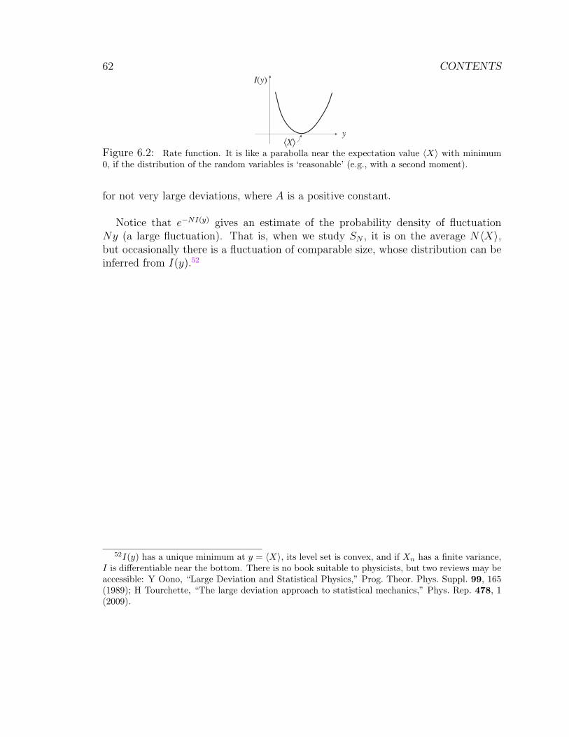
62 CONTENTS
y
I(y)
〈X〉Figure 6.2: Rate function. It is like a parabolla near the expectation value 〈X〉 with minimum0, if the distribution of the random variables is ‘reasonable’ (e.g., with a second moment).
for not very large deviations, where A is a positive constant.
Notice that e−NI(y) gives an estimate of the probability density of fluctuationNy (a large fluctuation). That is, when we study SN , it is on the average N〈X〉,but occasionally there is a fluctuation of comparable size, whose distribution can beinferred from I(y).52
52I(y) has a unique minimum at y = 〈X〉, its level set is convex, and if Xn has a finite variance,I is differentiable near the bottom. There is no book suitable to physicists, but two reviews may beaccessible: Y Oono, “Large Deviation and Statistical Physics,” Prog. Theor. Phys. Suppl. 99, 165(1989); H Tourchette, “The large deviation approach to statistical mechanics,” Phys. Rep. 478, 1(2009).
7. LECTURE 7: FLUCTUATION-DISSIPATION RELATION; EFFECT OF MANY MANY PARTICLES63
7 Lecture 7: Fluctuation-dissipation relation; Ef-
fect of many many particles
Summary∗ Since the Brownian motion is a mesoscale phenomenon and the long time mac-
robehavior corresponds to the results of the law of large numbers, large deviationframework is the natural theoretical tool to describe Brownian motions.
∗ This tells us that the noise in the Langevin equation must be Gaussian, and itsfluctuation amplitude is determined by the fluctuation-dissipation relation, whichis basically Einstein’s relation.
∗ If numerous particles gather, important observables are extensive (additive) or in-tensive. Also even though underlying mechanics is reversible, macroscopic sys-tems exhibit irreversibility.
∗ For a macroscopic system its total mechanical energy is additive with high precision.
Key wordsFluctuation-dissipation relation, Smoluchowski equation, internal energy, reversibil-ity of mechanics, Poincare recurrence
What you should be able to do∗ You must be able to set up a Langevin equation with a proper noise.∗ You should understand the ‘divide and conquer’ way of studying equations con-
sisting of several different types of dynamics.∗ You must be able to obtain the equilibrium distribution from the Smoluchowski
equation.∗ Explain why irreversibility naturally occurs in systems with many particles.
Let us study the overdamped Langevin equation that describes the motion of aBrownian particle. It is a mesoscopic level equation. Therefore, d/dt is not themicroscopic true derivative appearing in microscopic mechancis, but is a ‘coarse-grained’ derivative, so let us write it as
∆x
∆t=
1
ζF + X. (7.1)
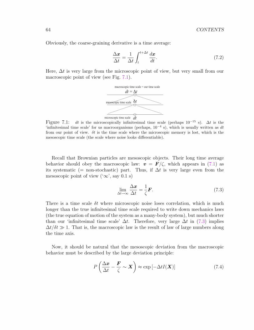
64 CONTENTS
Obviously, the coarse-graining derivative is a time average:
∆x
∆t=
1
∆t
∫ t+∆t
t
dx
dt. (7.2)
Here, ∆t is very large from the microscopic point of view, but very small from ourmacroscopic point of view (see Fig. 7.1).
macroscopic time scale = our time scale
dt = Δt
dt
δtmesoscopic time scale
microscopic time scale
Figure 7.1: dt is the microscopically infinitesimal time scale (perhaps 10−15 s). ∆t is the‘infinitesimal time scale’ for us macroorganisms (perhaps, 10−4 s), which is usually written as dtfrom our point of view. δt is the time scale where the microscopic memory is lost, which is themesoscopic time scale (the scale where noise looks differentiable).
Recall that Brownian particles are mesoscopic objects. Their long time averagebehavior should obey the macroscopic law: v = F /ζ, which appears in (7.1) asits systematic (= non-stochastic) part. Thus, if ∆t is very large even from themesoscopic point of view (‘∞’, say 0.1 s)
lim∆t→∞
∆x
∆t=
1
ζF . (7.3)
There is a time scale δt where microscopic noise loses correlation, which is muchlonger than the true infinitesimal time scale required to write down mechanics laws(the true equation of motion of the system as a many-body system), but much shorterthan our ‘infinitesimal time scale’ ∆t. Therefore, very large ∆t in (7.3) implies∆t/δt 1. That is, the macroscopic law is the result of law of large numbers alongthe time axis.
Now, it should be natural that the mesoscopic deviation from the macroscopicbehavior must be described by the large deviation principle:
P
(∆x
∆t− F
ζ∼X
)≈ exp [−∆tI(X)] (7.4)
7. LECTURE 7: FLUCTUATION-DISSIPATION RELATION; EFFECT OF MANY MANY PARTICLES65
with
I(X) =1
2AX2 (7.5)
for most fluctuations that are not terribly large (see Fig. 6.2). That is, we mayassume that the random force is Gaussian, and 〈X2〉 = A/∆t. Thus, A describesthe noise amplitude. One quick way to guess A is to compute the mean squaredisplacement during time ∆t without F :
〈x2〉 = ∆t2〈X2〉 = dA∆t. (7.6)
Here, d is the spatial dimensionality. This should be compared with Einstein’s re-sult;
A = 2D =2kBT
ζ. (7.7)
Since ζ describe the resistance due to the medium, it is a measure of dissipation.Therefore, the above relation is called the fluctuation-dissipation relation.
The fluctuation-dissipation relation is usually derived from the condition thatthe equilibrium distribution of the particles is correctly described by the Boltzmannfactor.53 Suppose F = −∇U , that is, the systematic force F is a conserved force witha potential U . Then, as we have already guessed, the equilibrium particle densitymust be proportional to e−βU . If a Brownian particle is trapped in a potential U ,it must obey this (density) distribution function. If the noise = random force Xis too wild (i.e., A in (7.5) is too large), then the distribution of the particle mustspread more than e−βU . On the other hand, if the noise is too small, then the particlewould be tightly trapped at the bottom of the potential. Thus, there must be the‘just-right’ noise amplitude (squared) A. It is given by (7.7), but here let us computethe equilibrium distribution with noise specified by (7.5).
Let N be the total number of Brownian particles. Then P (r, t) = n(r, t)/N ,where n(r, t) is the number density of the particles at time t around r, is understoodas the probability density distribution function of the Brownian particle. Let usderive an equation that governs the time evolution of this probability density.
We assume each particle obeys (7.1), which can be written as
dx = −1
ζ∇Udt+ Xdt. (7.8)
53Notice that even the above derivation imports the equilibrium result as the equipartition ofenergy or the formula for the pressure.
66 CONTENTS
This implies for a short time the dynamics is a superposition of two dynamics,systematic and stochastic. Thus, we can separate the short-time evolution dynamicsof P also into two parts, systematic and stochastic, and can consider them separately(both are proportional to dt so cross-terms are inevitably higher order).
The latter is diffusion as Einstein demonstrated, so we know the answer:
∂P
∂t=A
2∆P. (7.9)
Here ∆ is the Laplacian ∆ = div grad:
∆ =∂2
∂x2+
∂2
∂y2+
∂2
∂z2. (7.10)
Next, the systematic part: if particles moves according to
dx
dt= v, (7.11)
the particle flux (after normalization, probability flux) is Pv. The probability isconserved, so we have
∂P
∂t= −div (vP )
(∂P
∂t= −
∑i
∂
∂xi
(viP )
). (7.12)
Let us apply this to the systematic part:
∂P
∂t= div
(∇UζP
) (∂P
∂t=∑
i
∂
∂xi
(1
ζ
∂U
∂xi
P
)). (7.13)
Combining (7.9) and (7.13) we get
∂P
∂t= ∇ ·
(1
ζ(∇U) +
A
2∇)P
(∂P
∂t=∑
i
∂
∂xi
(1
ζ
∂U
∂xi
+A
2
∂
∂xi
)P
). (7.14)
This is called the Smoluchowski equation. In equilibrium, P should be time indepen-dent: (
1
ζ∇U +
A
2∇)P = const.
(1
ζ
∂U
∂xi
+A
2
∂
∂xi
logP = const.
). (7.15)
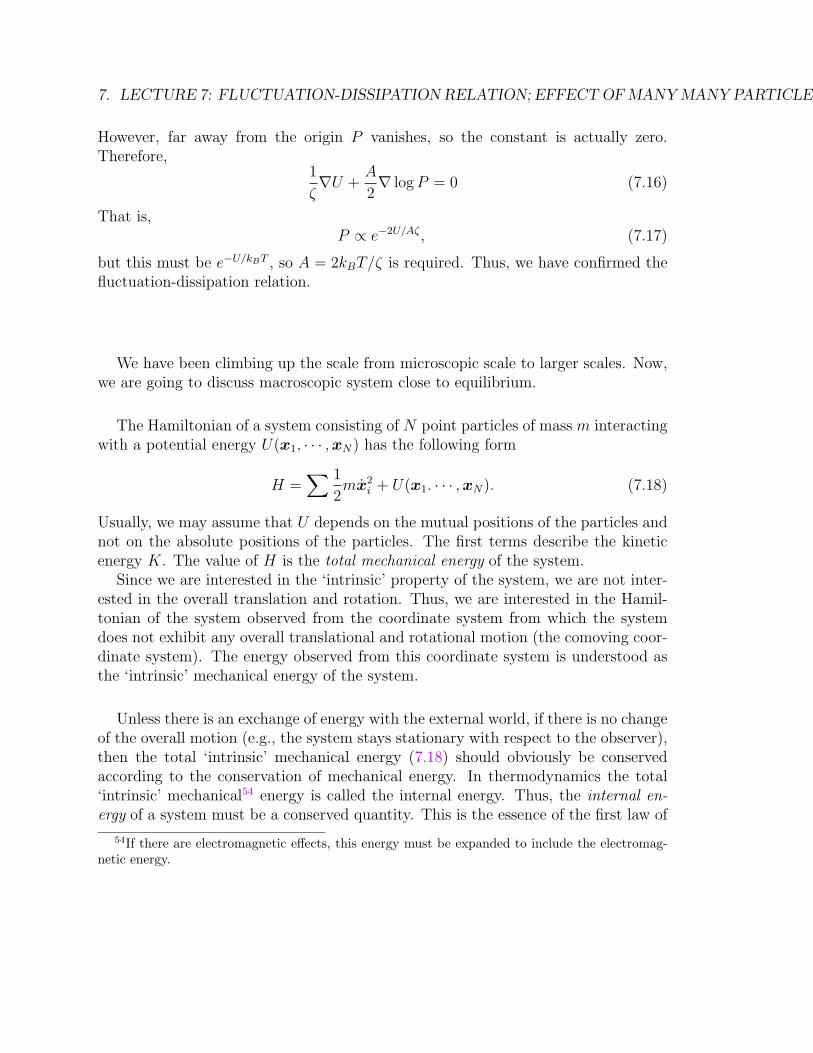
7. LECTURE 7: FLUCTUATION-DISSIPATION RELATION; EFFECT OF MANY MANY PARTICLES67
However, far away from the origin P vanishes, so the constant is actually zero.Therefore,
1
ζ∇U +
A
2∇ logP = 0 (7.16)
That is,P ∝ e−2U/Aζ , (7.17)
but this must be e−U/kBT , so A = 2kBT/ζ is required. Thus, we have confirmed thefluctuation-dissipation relation.
We have been climbing up the scale from microscopic scale to larger scales. Now,we are going to discuss macroscopic system close to equilibrium.
The Hamiltonian of a system consisting of N point particles of mass m interactingwith a potential energy U(x1, · · · ,xN) has the following form
H =∑ 1
2mx2
i + U(x1. · · · ,xN). (7.18)
Usually, we may assume that U depends on the mutual positions of the particles andnot on the absolute positions of the particles. The first terms describe the kineticenergy K. The value of H is the total mechanical energy of the system.
Since we are interested in the ‘intrinsic’ property of the system, we are not inter-ested in the overall translation and rotation. Thus, we are interested in the Hamil-tonian of the system observed from the coordinate system from which the systemdoes not exhibit any overall translational and rotational motion (the comoving coor-dinate system). The energy observed from this coordinate system is understood asthe ‘intrinsic’ mechanical energy of the system.
Unless there is an exchange of energy with the external world, if there is no changeof the overall motion (e.g., the system stays stationary with respect to the observer),then the total ‘intrinsic’ mechanical energy (7.18) should obviously be conservedaccording to the conservation of mechanical energy. In thermodynamics the total‘intrinsic’ mechanical54 energy is called the internal energy. Thus, the internal en-ergy of a system must be a conserved quantity. This is the essence of the first law of
54If there are electromagnetic effects, this energy must be expanded to include the electromag-netic energy.
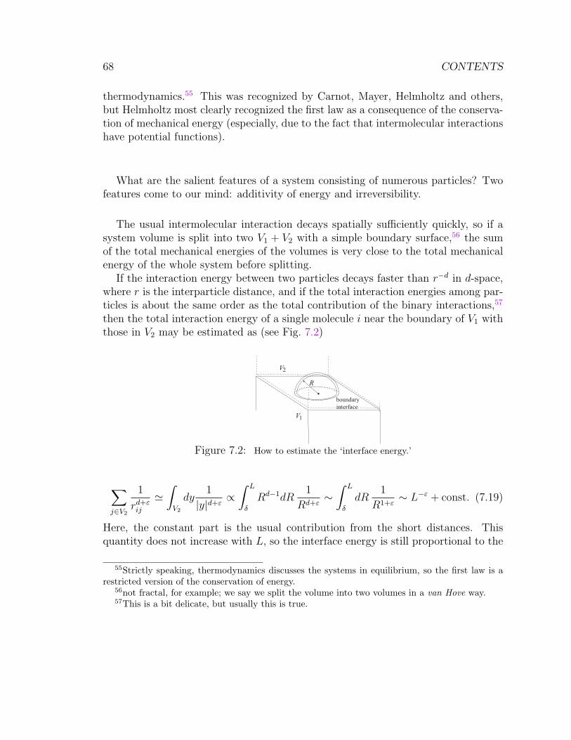
68 CONTENTS
thermodynamics.55 This was recognized by Carnot, Mayer, Helmholtz and others,but Helmholtz most clearly recognized the first law as a consequence of the conserva-tion of mechanical energy (especially, due to the fact that intermolecular interactionshave potential functions).
What are the salient features of a system consisting of numerous particles? Twofeatures come to our mind: additivity of energy and irreversibility.
The usual intermolecular interaction decays spatially sufficiently quickly, so if asystem volume is split into two V1 + V2 with a simple boundary surface,56 the sumof the total mechanical energies of the volumes is very close to the total mechanicalenergy of the whole system before splitting.
If the interaction energy between two particles decays faster than r−d in d-space,where r is the interparticle distance, and if the total interaction energies among par-ticles is about the same order as the total contribution of the binary interactions,57
then the total interaction energy of a single molecule i near the boundary of V1 withthose in V2 may be estimated as (see Fig. 7.2)
R
V
V1
2
boundary
interface
Figure 7.2: How to estimate the ‘interface energy.’
∑j∈V2
1
rd+εij
'∫
V2
dy1
|y|d+ε∝∫ L
δ
Rd−1dR1
Rd+ε∼∫ L
δ
dR1
R1+ε∼ L−ε + const. (7.19)
Here, the constant part is the usual contribution from the short distances. Thisquantity does not increase with L, so the interface energy is still proportional to the
55Strictly speaking, thermodynamics discusses the systems in equilibrium, so the first law is arestricted version of the conservation of energy.
56not fractal, for example; we say we split the volume into two volumes in a van Hove way.57This is a bit delicate, but usually this is true.

7. LECTURE 7: FLUCTUATION-DISSIPATION RELATION; EFFECT OF MANY MANY PARTICLES69
surface area of the interface Ld−1.Thus, if the interaction potential decays faster than r−d, then we may assume that
the total energy is proportional to the volume of the system.The Coulomb and gravitational interaction energies decay as 1/r. For the Coulomb
interaction, thanks to the shielding effect, if the system is charge-neutral, the effec-tive interaction decays exponentially, so we need not worry about it. For the gravity,there is no way to shield it, but the usual macroscopic objects we are interestedin in statistical physics is not huge (usually about 1 m3 or less with not a hugedensity like a neutron star), so we may ignore it (unless we discuss sedimentationequilibrium).58
To study a macroscopic system we often study additive observables that is pro-portional to the system size (think of internal energy). This is natural, because suchobservables are big for big systems. If an observable becomes smaller for larger sys-tems, we need not pay attention to such quantities to understand the macroscopicworld. Thus, we are interested in observables that are independent of the systemsize (intensive quantities) and those proportional to the amount of materials in thesystem (extensive quantities).
The world of mechanics is time-reversal symmetric. This implies that even ifa movie of a mechanical phenomenon is played backward in time (t → −t), thephenomenon we can watch in the movie obeys the same equation of motion. Inthe case of classical mechanics, Newton’s equation of motion of a closed (isolated)system is an autonomous differential equation of second order without any first orderderivative: For an N -particle system, generally we have
d2xi
dt2= F i(x1, · · · ,xN) (7.20)
for i = 1, · · · , N . Since the forces F i are t independent in the closed system, t→ −tdoes not change the equations.
The Schrodinger equation for an isolated system reads
i~∂ψ
∂t= Hψ, (7.21)
where H is a Hermitian operator independent of time. In this case t → −t mightseem to alter physics, but what we observe is real, so the physics must be intact under
58If the system really becomes huge, our ordinary statistical thermodynamics does not work.
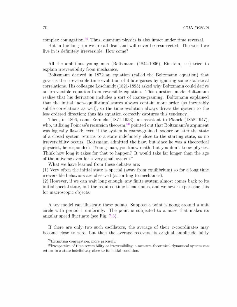
70 CONTENTS
complex conjugation.59 Thus, quantum physics is also intact under time reversal.But in the long run we are all dead and will never be resurrected. The world we
live in is definitely irreversible. How come?
All the ambitious young men (Boltzmann (1844-1906), Einstein, · · ·) tried toexplain irreversibility from mechanics.
Boltzmann derived in 1872 an equation (called the Boltzmann equation) thatgoverns the irreversible time evolution of dilute gasses by ignoring some statisticalcorrelations. His colleague Loschmidt (1821-1895) asked why Boltzmann could derivean irreversible equation from reversible equation. This question made Boltzmannrealize that his derivation includes a sort of coarse-graining. Boltzmann explainedthat the initial ‘non-equilibrium’ states always contain more order (so inevitablysubtle correlations as well), so the time evolution always drives the system to theless ordered direction; thus his equation correctly captures this tendency.
Then, in 1896, came Zermelo (1871-1953), an assistant to Planck (1858-1947),who, utilizing Poincae’s recursion theorem,60 pointed out that Boltzmann’s argumentwas logically flawed: even if the system is coarse-grained, sooner or later the stateof a closed system returns to a state indefinitely close to the starting state, so noirreversibility occurs. Boltzmann admitted the flaw, but since he was a theoreticalphysicist, he responded: “Young man, you know math, but you don’t know physics.Think how long it takes for that to happen? It would take far longer than the ageof the universe even for a very small system.”
What we have learned from these debates are:(1) Very often the initial state is special (away from equilibrium) so for a long timeirreversible behaviors are observed (according to mechanics).(2) However, if we can wait long enough, any finite system almost comes back to itsinitial special state, but the required time is enormous, and we never experiecne thisfor macroscopic objects.
A toy model can illustrate these points. Suppose a point is going around a unitcircle with period 1 uniformly. The point is subjected to a noise that makes itsangular speed fluctuate (see Fig. 7.3).
If there are only two such oscillators, the average of their x-coordinates maybecome close to zero, but then the average recovers its original amplitude fairly
59Hermitian conjugation, more precisely.60Irrespective of time reversibility or irreversibility, a measure-theoretical dynamical system can
return to a state indefinitely close to its initial condition.
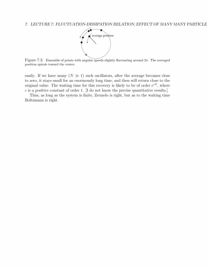
7. LECTURE 7: FLUCTUATION-DISSIPATION RELATION; EFFECT OF MANY MANY PARTICLES71
average position
Figure 7.3: Ensemble of points with angular speeds slightly fluctuating around 2π. The averagedposition spirals toward the center.
easily. If we have many (N 1) such oscillators, after the average becomes closeto zero, it stays small for an enormously long time, and then will return close to theoriginal value. The waiting time for this recovery is likely to be of order ecN , wherec is a positive constant of order 1. [I do not know the precise quantitative results.]
Thus, as long as the system is finite, Zermelo is right, but as to the waiting timeBoltzmann is right.
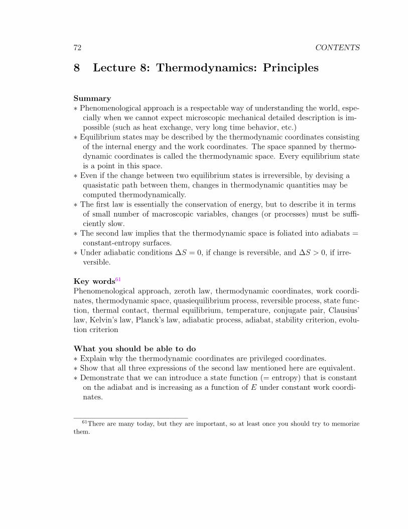
72 CONTENTS
8 Lecture 8: Thermodynamics: Principles
Summary∗ Phenomenological approach is a respectable way of understanding the world, espe-
cially when we cannot expect microscopic mechanical detailed description is im-possible (such as heat exchange, very long time behavior, etc.)
∗ Equilibrium states may be described by the thermodynamic coordinates consistingof the internal energy and the work coordinates. The space spanned by thermo-dynamic coordinates is called the thermodynamic space. Every equilibrium stateis a point in this space.
∗ Even if the change between two equilibrium states is irreversible, by devising aquasistatic path between them, changes in thermodynamic quantities may becomputed thermodynamically.
∗ The first law is essentially the conservation of energy, but to describe it in termsof small number of macroscopic variables, changes (or processes) must be suffi-ciently slow.
∗ The second law implies that the thermodynamic space is foliated into adiabats =constant-entropy surfaces.
∗ Under adiabatic conditions ∆S = 0, if change is reversible, and ∆S > 0, if irre-versible.
Key words61
Phenomenological approach, zeroth law, thermodynamic coordinates, work coordi-nates, thermodynamic space, quasiequilibrium process, reversible process, state func-tion, thermal contact, thermal equilibrium, temperature, conjugate pair, Clausius’law, Kelvin’s law, Planck’s law, adiabatic process, adiabat, stability criterion, evolu-tion criterion
What you should be able to do∗ Explain why the thermodynamic coordinates are privileged coordinates.∗ Show that all three expressions of the second law mentioned here are equivalent.∗ Demonstrate that we can introduce a state function (= entropy) that is constant
on the adiabat and is increasing as a function of E under constant work coordi-nates.
61There are many today, but they are important, so at least once you should try to memorizethem.
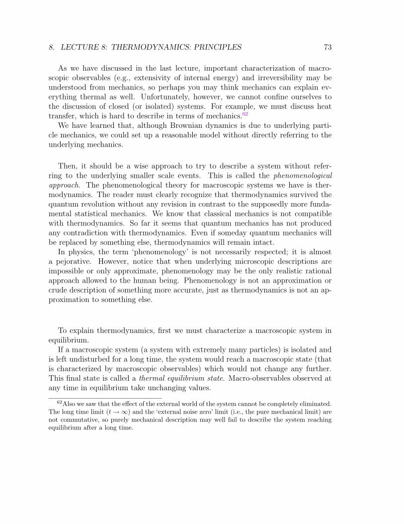
8. LECTURE 8: THERMODYNAMICS: PRINCIPLES 73
As we have discussed in the last lecture, important characterization of macro-scopic observables (e.g., extensivity of internal energy) and irreversibility may beunderstood from mechanics, so perhaps you may think mechanics can explain ev-erything thermal as well. Unfortunately, however, we cannot confine ourselves tothe discussion of closed (or isolated) systems. For example, we must discuss heattransfer, which is hard to describe in terms of mechanics.62
We have learned that, although Brownian dynamics is due to underlying parti-cle mechanics, we could set up a reasonable model without directly referring to theunderlying mechanics.
Then, it should be a wise approach to try to describe a system without refer-ring to the underlying smaller scale events. This is called the phenomenologicalapproach. The phenomenological theory for macroscopic systems we have is ther-modynamics. The reader must clearly recognize that thermodynamics survived thequantum revolution without any revision in contrast to the supposedly more funda-mental statistical mechanics. We know that classical mechanics is not compatiblewith thermodynamics. So far it seems that quantum mechanics has not producedany contradiction with thermodynamics. Even if someday quantum mechanics willbe replaced by something else, thermodynamics will remain intact.
In physics, the term ‘phenomenology’ is not necessarily respected; it is almosta pejorative. However, notice that when underlying microscopic descriptions areimpossible or only approximate, phenomenology may be the only realistic rationalapproach allowed to the human being. Phenomenology is not an approximation orcrude description of something more accurate, just as thermodynamics is not an ap-proximation to something else.
To explain thermodynamics, first we must characterize a macroscopic system inequilibrium.
If a macroscopic system (a system with extremely many particles) is isolated andis left undisturbed for a long time, the system would reach a macroscopic state (thatis characterized by macroscopic observables) which would not change any further.This final state is called a thermal equilibrium state. Macro-observables observed atany time in equilibrium take unchanging values.
62Also we saw that the effect of the external world of the system cannot be completely eliminated.The long time limit (t→∞) and the ‘external noise zero’ limit (i.e., the pure mechanical limit) arenot commutative, so purely mechanical description may well fail to describe the system reachingequilibrium after a long time.
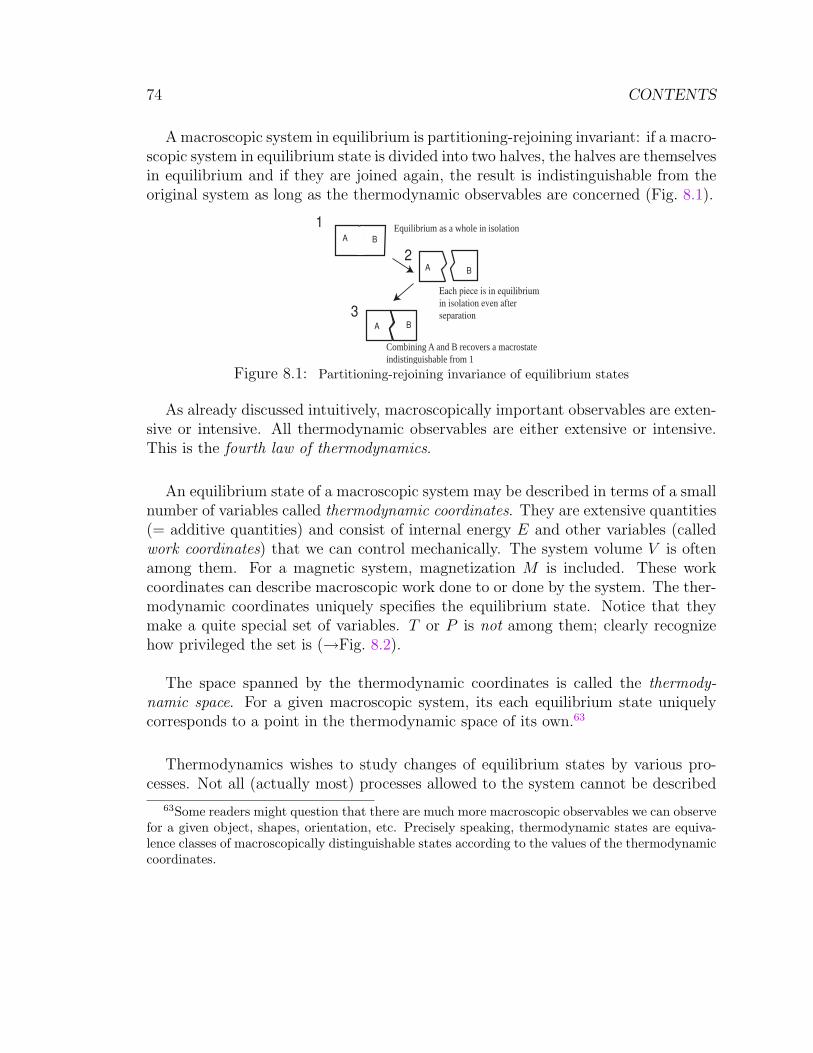
74 CONTENTS
A macroscopic system in equilibrium is partitioning-rejoining invariant: if a macro-scopic system in equilibrium state is divided into two halves, the halves are themselvesin equilibrium and if they are joined again, the result is indistinguishable from theoriginal system as long as the thermodynamic observables are concerned (Fig. 8.1).
Equilibrium as a whole in isolation
Each piece is in equilibrium
in isolation even after
separation
Combining A and B recovers a macrostateindistinguishable from 1
A B
A B
A B
1
2
3
Figure 8.1: Partitioning-rejoining invariance of equilibrium states
As already discussed intuitively, macroscopically important observables are exten-sive or intensive. All thermodynamic observables are either extensive or intensive.This is the fourth law of thermodynamics.
An equilibrium state of a macroscopic system may be described in terms of a smallnumber of variables called thermodynamic coordinates. They are extensive quantities(= additive quantities) and consist of internal energy E and other variables (calledwork coordinates) that we can control mechanically. The system volume V is oftenamong them. For a magnetic system, magnetization M is included. These workcoordinates can describe macroscopic work done to or done by the system. The ther-modynamic coordinates uniquely specifies the equilibrium state. Notice that theymake a quite special set of variables. T or P is not among them; clearly recognizehow privileged the set is (→Fig. 8.2).
The space spanned by the thermodynamic coordinates is called the thermody-namic space. For a given macroscopic system, its each equilibrium state uniquelycorresponds to a point in the thermodynamic space of its own.63
Thermodynamics wishes to study changes of equilibrium states by various pro-cesses. Not all (actually most) processes allowed to the system cannot be described
63Some readers might question that there are much more macroscopic observables we can observefor a given object, shapes, orientation, etc. Precisely speaking, thermodynamic states are equiva-lence classes of macroscopically distinguishable states according to the values of the thermodynamiccoordinates.
8. LECTURE 8: THERMODYNAMICS: PRINCIPLES 75
A B C
Figure 8.2: A-C are the same amount of water at 0C. However, their internal energies aredistinct; A has less than C. In elementary thermodynamics, often the temperature T appears as akey variable instead of internal energy E, but these examples clearly tell us that T cannot distinguishequilibrium states that are clearly distinct. Analogously, in the liquid-gas phase transition underconstant pressure P and T , E and V change. These examples clearly indicate that thermodynamiccoordinates are the fundamental ‘privileged’ set of variables to describe thermodynamic equilibriumstate; generally speaking intensive variables such as T and P fail to describe states uniquely.
in the thermodynamic space, because every point actually realizable in the thermo-dynamic space describes an equilibrium state of the system. Only processes that areextremely (infinitesimally) close (experimentally indistinguishably close) to equilib-rium states at every moment may be expressed as a continuous curve in the thermo-dynamic space. Such processes are called quasistatic processes. A quasistatic processis synonymous to a process that has a curve representation in the thermodynamicspace (Fig. 8.3).
A
B
quasistatic
noneq process
equilibrium states
thermodynamic
space
Figure 8.3: A and B are equilibrium states. A quasistatic process connecting A and B is in thethermodynamic space. From A to B a process need not be quasistatic. Then, such a process cannotbe described in the thermodynamic space (red).
Whether it is reversible (retraceable) or not is not directly related to quasistaticnature (being slow or not) of the process,64 although not quasistatic processes arevery likely to be irreversible.
Certainly, the processes not described as curves in the thermodynamic space are
64Think of a hot coffee in a thermos.Whether a given quasistatic process is reversible or not depends on the context. In the case of
thermos, the process is undoubtedly irreversible. However, you could cool your coffee by removingheat reversibly by producing work
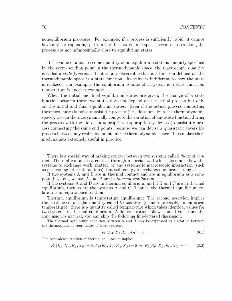
76 CONTENTS
nonequilibrium processes. For example, if a process is sufficiently rapid, it cannothave any corresponding path in the thermodynamic space, because states along theprocess are not infinitesimally close to equilibrium states.
If the value of a macroscopic quantity of an equilibrium state is uniquely specifiedby the corresponding point in the thermodynamic space, the macroscopic quantityis called a state function.. That is, any observable that is a function defined on thethermodynamic space is a state function. Its value is indifferent to how the stateis realized. For example, the equilibrium volume of a system is a state function;temperature is another example.
When the initial and final equilibrium states are given, the change of a statefunction between these two states does not depend on the actual process but onlyon the initial and final equilibrium states. Even if the actual process connectingthese two states is not a quasistatic process (i.e., does not lie in the thermodynamicspace), we can thermodynamically compute the variation of any state function duringthe process with the aid of an appropriate (appropriately devised) quasistatic pro-cess connecting the same end points, because we can devise a quasistatic reversibleprocess between any realizable points in the thermodynamic space. This makes ther-modynamics extremely useful in practice.
There is a special way of making contact between two systems called thermal con-tact. Thermal contact is a contact through a special wall which does not allow thesystems to exchange work, matter, or any systematic macroscopic interaction (suchas electromagnetic interactions), but still energy is exchanged as heat through it.
If two systems A and B are in thermal contact and are in equilibrium as a com-pound system, we say A and B are in thermal equilibrium.
If the systems A and B are in thermal equilibrium, and if B and C are in thermalequilibrium, then so are the systems A and C. That is, the thermal equilibrium re-lation is an equivalence relation.
Thermal equilibrium is temperature equilibrium: The second assertion impliesthe existence of a scalar quantity called temperature (or more precisely, an empiricaltemperature): there is a quantity called temperature which takes identical values fortwo systems in thermal equilibrium. A demonstration follows, but if you think theconclusion is natural, you can skip the following fine-lettered discussion.
The thermal equilibrium condition between A and B may be expressed as a relation betweenthe thermodynamic coordinates of these systems:
FC(EA, XA, EB , XB) = 0. (8.1)
The equivalence relation of thermal equilibrium implies
FC(EA, XA, EB , XB) = 0, FB(EC , XC , EA, XA) = 0 ⇒ FA(EB , XB , EC , XC) = 0. (8.2)
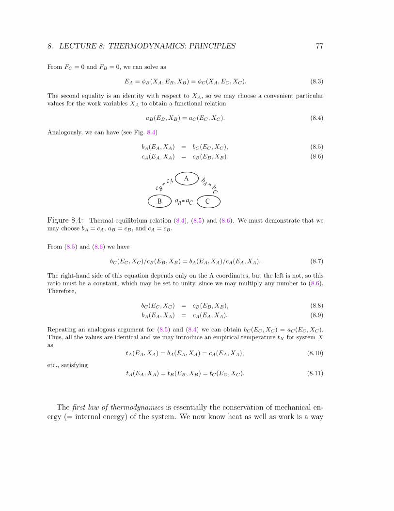
8. LECTURE 8: THERMODYNAMICS: PRINCIPLES 77
From FC = 0 and FB = 0, we can solve as
EA = φB(XA, EB , XB) = φC(XA, EC , XC). (8.3)
The second equality is an identity with respect to XA, so we may choose a convenient particularvalues for the work variables XA to obtain a functional relation
aB(EB , XB) = aC(EC , XC). (8.4)
Analogously, we can have (see Fig. 8.4)
bA(EA, XA) = bC(EC , XC), (8.5)cA(EA, XA) = cB(EB , XB). (8.6)
A
B Ca
bc
a
bc
A
B C
A
B C
= =
=
Figure 8.4: Thermal equilibrium relation (8.4), (8.5) and (8.6). We must demonstrate that wemay choose bA = cA, aB = cB , and cA = cB .
From (8.5) and (8.6) we have
bC(EC , XC)/cB(EB , XB) = bA(EA, XA)/cA(EA, XA). (8.7)
The right-hand side of this equation depends only on the A coordinates, but the left is not, so thisratio must be a constant, which may be set to unity, since we may multiply any number to (8.6).Therefore,
bC(EC , XC) = cB(EB , XB), (8.8)bA(EA, XA) = cA(EA, XA). (8.9)
Repeating an analogous argument for (8.5) and (8.4) we can obtain bC(EC , XC) = aC(EC , XC).Thus, all the values are identical and we may introduce an empirical temperature tX for system Xas
tA(EA, XA) = bA(EA, XA) = cA(EA, XA), (8.10)
etc., satisfyingtA(EA, XA) = tB(EB , XB) = tC(EC , XC). (8.11)
The first law of thermodynamics is essentially the conservation of mechanical en-ergy (= internal energy) of the system. We now know heat as well as work is a way
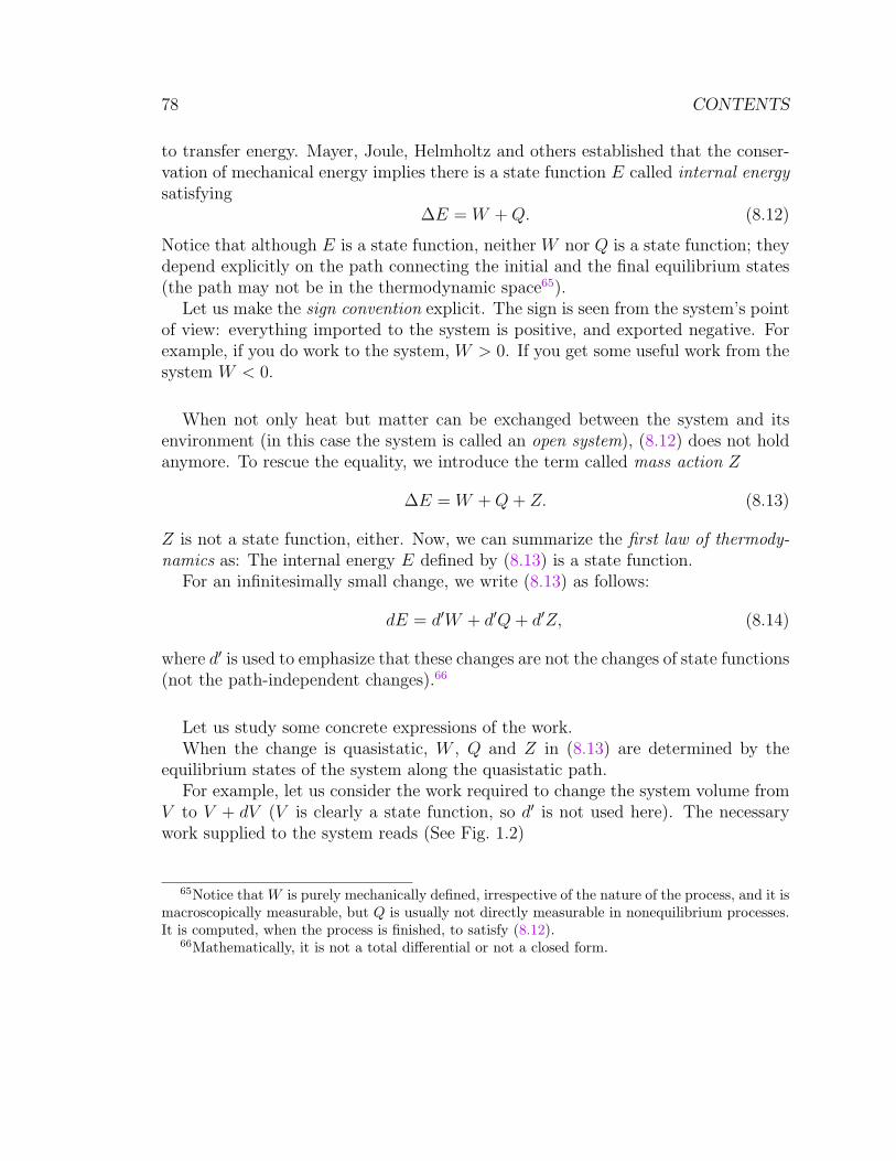
78 CONTENTS
to transfer energy. Mayer, Joule, Helmholtz and others established that the conser-vation of mechanical energy implies there is a state function E called internal energysatisfying
∆E = W +Q. (8.12)
Notice that although E is a state function, neither W nor Q is a state function; theydepend explicitly on the path connecting the initial and the final equilibrium states(the path may not be in the thermodynamic space65).
Let us make the sign convention explicit. The sign is seen from the system’s pointof view: everything imported to the system is positive, and exported negative. Forexample, if you do work to the system, W > 0. If you get some useful work from thesystem W < 0.
When not only heat but matter can be exchanged between the system and itsenvironment (in this case the system is called an open system), (8.12) does not holdanymore. To rescue the equality, we introduce the term called mass action Z
∆E = W +Q+ Z. (8.13)
Z is not a state function, either. Now, we can summarize the first law of thermody-namics as: The internal energy E defined by (8.13) is a state function.
For an infinitesimally small change, we write (8.13) as follows:
dE = d′W + d′Q+ d′Z, (8.14)
where d′ is used to emphasize that these changes are not the changes of state functions(not the path-independent changes).66
Let us study some concrete expressions of the work.When the change is quasistatic, W , Q and Z in (8.13) are determined by the
equilibrium states of the system along the quasistatic path.For example, let us consider the work required to change the system volume from
V to V + dV (V is clearly a state function, so d′ is not used here). The necessarywork supplied to the system reads (See Fig. 1.2)
65Notice that W is purely mechanically defined, irrespective of the nature of the process, and it ismacroscopically measurable, but Q is usually not directly measurable in nonequilibrium processes.It is computed, when the process is finished, to satisfy (8.12).
66Mathematically, it is not a total differential or not a closed form.
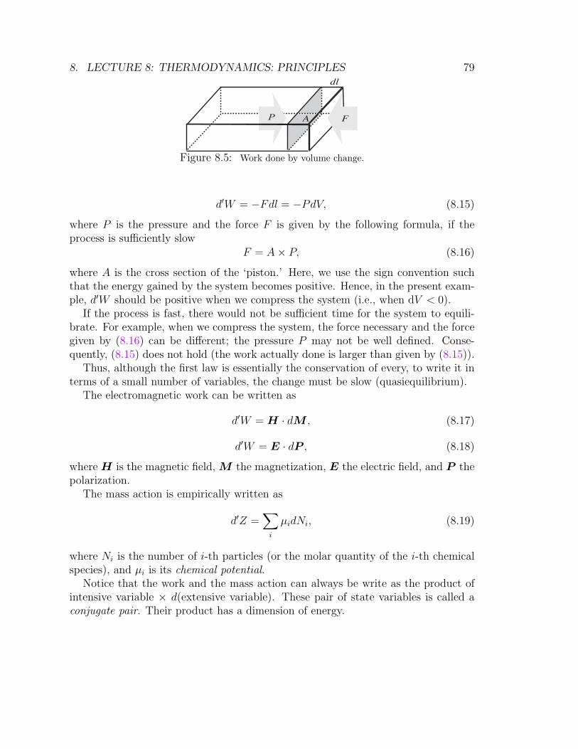
8. LECTURE 8: THERMODYNAMICS: PRINCIPLES 79dl
AP F
Figure 8.5: Work done by volume change.
d′W = −Fdl = −PdV, (8.15)
where P is the pressure and the force F is given by the following formula, if theprocess is sufficiently slow
F = A× P, (8.16)
where A is the cross section of the ‘piston.’ Here, we use the sign convention suchthat the energy gained by the system becomes positive. Hence, in the present exam-ple, d′W should be positive when we compress the system (i.e., when dV < 0).
If the process is fast, there would not be sufficient time for the system to equili-brate. For example, when we compress the system, the force necessary and the forcegiven by (8.16) can be different; the pressure P may not be well defined. Conse-quently, (8.15) does not hold (the work actually done is larger than given by (8.15)).
Thus, although the first law is essentially the conservation of every, to write it interms of a small number of variables, the change must be slow (quasiequilibrium).
The electromagnetic work can be written as
d′W = H · dM , (8.17)
d′W = E · dP , (8.18)
where H is the magnetic field, M the magnetization, E the electric field, and P thepolarization.
The mass action is empirically written as
d′Z =∑
i
µidNi, (8.19)
where Ni is the number of i-th particles (or the molar quantity of the i-th chemicalspecies), and µi is its chemical potential.
Notice that the work and the mass action can always be write as the product ofintensive variable × d(extensive variable). These pair of state variables is called aconjugate pair. Their product has a dimension of energy.
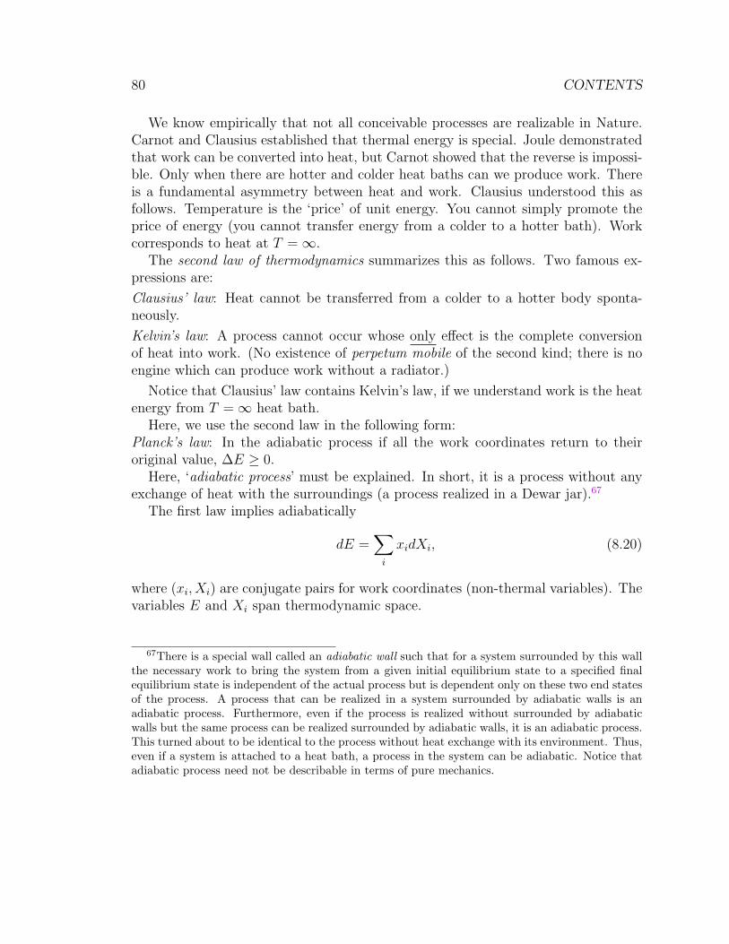
80 CONTENTS
We know empirically that not all conceivable processes are realizable in Nature.Carnot and Clausius established that thermal energy is special. Joule demonstratedthat work can be converted into heat, but Carnot showed that the reverse is impossi-ble. Only when there are hotter and colder heat baths can we produce work. Thereis a fundamental asymmetry between heat and work. Clausius understood this asfollows. Temperature is the ‘price’ of unit energy. You cannot simply promote theprice of energy (you cannot transfer energy from a colder to a hotter bath). Workcorresponds to heat at T =∞.
The second law of thermodynamics summarizes this as follows. Two famous ex-pressions are:
Clausius’ law: Heat cannot be transferred from a colder to a hotter body sponta-neously.
Kelvin’s law: A process cannot occur whose only effect is the complete conversionof heat into work. (No existence of perpetum mobile of the second kind; there is noengine which can produce work without a radiator.)
Notice that Clausius’ law contains Kelvin’s law, if we understand work is the heatenergy from T =∞ heat bath.
Here, we use the second law in the following form:Planck’s law: In the adiabatic process if all the work coordinates return to theiroriginal value, ∆E ≥ 0.
Here, ‘adiabatic process’ must be explained. In short, it is a process without anyexchange of heat with the surroundings (a process realized in a Dewar jar).67
The first law implies adiabatically
dE =∑
i
xidXi, (8.20)
where (xi, Xi) are conjugate pairs for work coordinates (non-thermal variables). Thevariables E and Xi span thermodynamic space.
67There is a special wall called an adiabatic wall such that for a system surrounded by this wallthe necessary work to bring the system from a given initial equilibrium state to a specified finalequilibrium state is independent of the actual process but is dependent only on these two end statesof the process. A process that can be realized in a system surrounded by adiabatic walls is anadiabatic process. Furthermore, even if the process is realized without surrounded by adiabaticwalls but the same process can be realized surrounded by adiabatic walls, it is an adiabatic process.This turned about to be identical to the process without heat exchange with its environment. Thus,even if a system is attached to a heat bath, a process in the system can be adiabatic. Notice thatadiabatic process need not be describable in terms of pure mechanics.
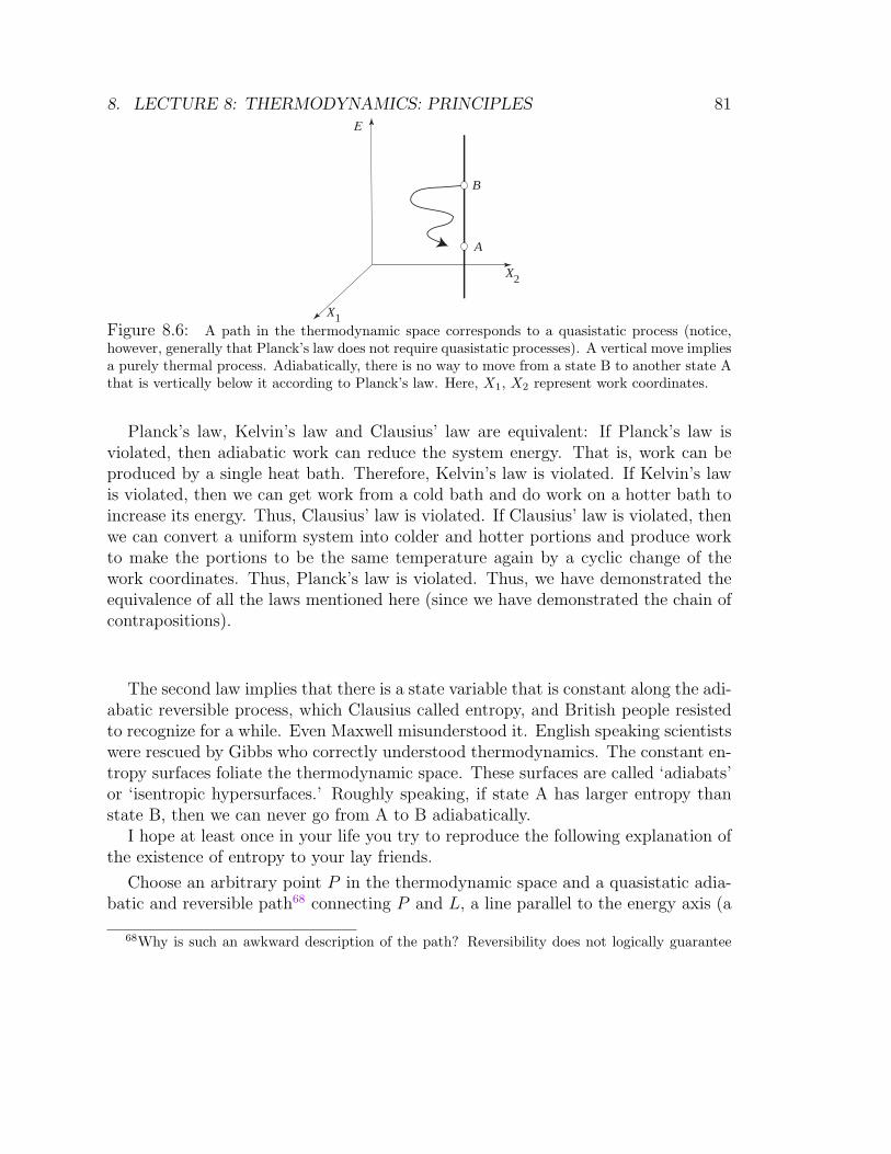
8. LECTURE 8: THERMODYNAMICS: PRINCIPLES 81
A
B
X
X
E
1
2
Figure 8.6: A path in the thermodynamic space corresponds to a quasistatic process (notice,however, generally that Planck’s law does not require quasistatic processes). A vertical move impliesa purely thermal process. Adiabatically, there is no way to move from a state B to another state Athat is vertically below it according to Planck’s law. Here, X1, X2 represent work coordinates.
Planck’s law, Kelvin’s law and Clausius’ law are equivalent: If Planck’s law isviolated, then adiabatic work can reduce the system energy. That is, work can beproduced by a single heat bath. Therefore, Kelvin’s law is violated. If Kelvin’s lawis violated, then we can get work from a cold bath and do work on a hotter bath toincrease its energy. Thus, Clausius’ law is violated. If Clausius’ law is violated, thenwe can convert a uniform system into colder and hotter portions and produce workto make the portions to be the same temperature again by a cyclic change of thework coordinates. Thus, Planck’s law is violated. Thus, we have demonstrated theequivalence of all the laws mentioned here (since we have demonstrated the chain ofcontrapositions).
The second law implies that there is a state variable that is constant along the adi-abatic reversible process, which Clausius called entropy, and British people resistedto recognize for a while. Even Maxwell misunderstood it. English speaking scientistswere rescued by Gibbs who correctly understood thermodynamics. The constant en-tropy surfaces foliate the thermodynamic space. These surfaces are called ‘adiabats’or ‘isentropic hypersurfaces.’ Roughly speaking, if state A has larger entropy thanstate B, then we can never go from A to B adiabatically.
I hope at least once in your life you try to reproduce the following explanation ofthe existence of entropy to your lay friends.
Choose an arbitrary point P in the thermodynamic space and a quasistatic adia-batic and reversible path68 connecting P and L, a line parallel to the energy axis (a
68Why is such an awkward description of the path? Reversibility does not logically guarantee
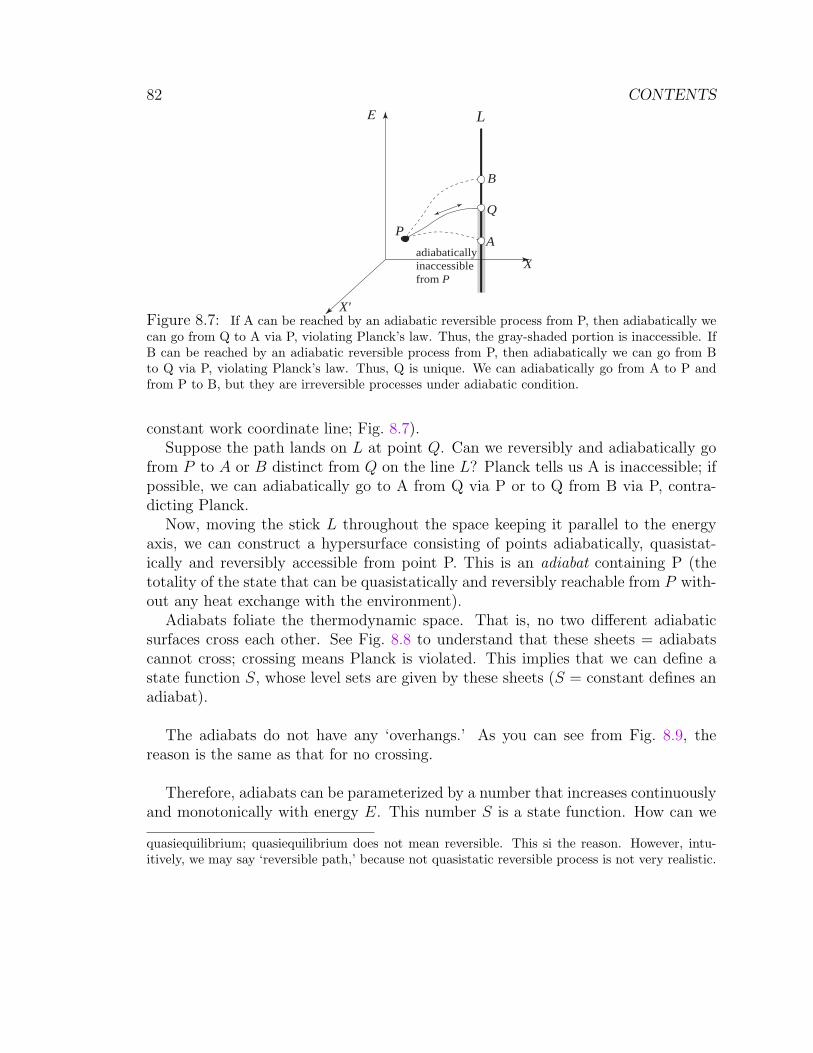
82 CONTENTS
P
Q
A
B
L
X
X'
E
adiabaticallyinaccessiblefrom P
Figure 8.7: If A can be reached by an adiabatic reversible process from P, then adiabatically wecan go from Q to A via P, violating Planck’s law. Thus, the gray-shaded portion is inaccessible. IfB can be reached by an adiabatic reversible process from P, then adiabatically we can go from Bto Q via P, violating Planck’s law. Thus, Q is unique. We can adiabatically go from A to P andfrom P to B, but they are irreversible processes under adiabatic condition.
constant work coordinate line; Fig. 8.7).Suppose the path lands on L at point Q. Can we reversibly and adiabatically go
from P to A or B distinct from Q on the line L? Planck tells us A is inaccessible; ifpossible, we can adiabatically go to A from Q via P or to Q from B via P, contra-dicting Planck.
Now, moving the stick L throughout the space keeping it parallel to the energyaxis, we can construct a hypersurface consisting of points adiabatically, quasistat-ically and reversibly accessible from point P. This is an adiabat containing P (thetotality of the state that can be quasistatically and reversibly reachable from P with-out any heat exchange with the environment).
Adiabats foliate the thermodynamic space. That is, no two different adiabaticsurfaces cross each other. See Fig. 8.8 to understand that these sheets = adiabatscannot cross; crossing means Planck is violated. This implies that we can define astate function S, whose level sets are given by these sheets (S = constant defines anadiabat).
The adiabats do not have any ‘overhangs.’ As you can see from Fig. 8.9, thereason is the same as that for no crossing.
Therefore, adiabats can be parameterized by a number that increases continuouslyand monotonically with energy E. This number S is a state function. How can we
quasiequilibrium; quasiequilibrium does not mean reversible. This si the reason. However, intu-itively, we may say ‘reversible path,’ because not quasistatic reversible process is not very realistic.
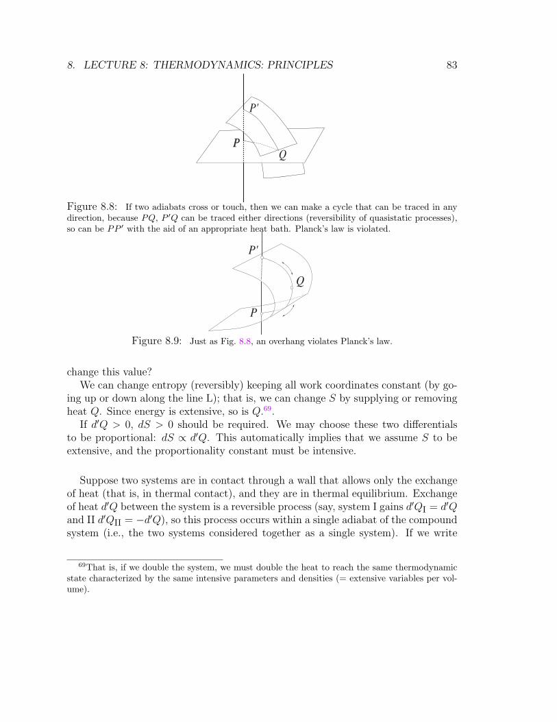
8. LECTURE 8: THERMODYNAMICS: PRINCIPLES 83
P'
PQ
Figure 8.8: If two adiabats cross or touch, then we can make a cycle that can be traced in anydirection, because PQ, P ′Q can be traced either directions (reversibility of quasistatic processes),so can be PP ′ with the aid of an appropriate heat bath. Planck’s law is violated.
P
Q
P'
Figure 8.9: Just as Fig. 8.8, an overhang violates Planck’s law.
change this value?We can change entropy (reversibly) keeping all work coordinates constant (by go-
ing up or down along the line L); that is, we can change S by supplying or removingheat Q. Since energy is extensive, so is Q.69.
If d′Q > 0, dS > 0 should be required. We may choose these two differentialsto be proportional: dS ∝ d′Q. This automatically implies that we assume S to beextensive, and the proportionality constant must be intensive.
Suppose two systems are in contact through a wall that allows only the exchangeof heat (that is, in thermal contact), and they are in thermal equilibrium. Exchangeof heat d′Q between the system is a reversible process (say, system I gains d′QI = d′Qand II d′QII = −d′Q), so this process occurs within a single adiabat of the compoundsystem (i.e., the two systems considered together as a single system). If we write
69That is, if we double the system, we must double the heat to reach the same thermodynamicstate characterized by the same intensive parameters and densities (= extensive variables per vol-ume).
84 CONTENTS
d′QX = θXdSX (X = I or II),
0 = dSI + dSII = d′Q
(1
θI− 1
θII
). (8.21)
This implies θI = θII. That is, when two systems have the same temperature, theproportionality constants are also the same. Hence, we may interpret the propor-tionality factor as a temperature (cf. the zeroth law).70
The introduced temperature can be chosen as a universal temperature T calledthe absolute temperature. Hence, in the quasistatic process we can write71
d′Q = TdS. (8.22)
Now we can write down the infinitesimal version of the first law of thermodynamicsfor the quasistatic process as follows:
dE = TdS − PdV + µdN + H · dM + · · · . (8.23)
This is called the Gibbs relation. because it was first written down by Gibbs. Noticethat each term consists of a product of a conjugate pair: an intensive factor andd[the corresponding (i.e., conjugate) extensive quantity].
Suppose a (perhaps compound) system is in equilibrium. If we modify its ex-ternal field (say, the electric field), its volume, or if we remove a wall between thesubsystems, the equilibrium state of the system may or may not change. Since allspontaneous processes are irreversible, we may say that for a system to change (underan adiabatic or isolated condition) from an initial state to a final state, the entropychange (which is completely determined by these end points in equilibrium) mustbe positive. If not, there cannot be any spontaneous change. Thus, for an isolatedsystem
∆S < 0 ⇐⇒ the state is thermodynamically stable, (8.24)
∆S > 0 ⇐⇒ the state spontaneously evolves. (8.25)
Therefore, the second law gives us a variational principle (entropy maximizationprinciple) to find a stable equilibrium state for an isolated system.72
70If you do not like this explanation, go to a much more complicated standard argument in theposted lecture notes.
71Precisely speaking, we must show that this T is identical to the T appearing in the ideal gaslaw.
72We will return to the system stability question in Chapter 4.

9. LECTURE 9: THERMODYNAMICS: GENERAL CONSEQUENCES 85
9 Lecture 9: Thermodynamics: General conse-
quences
Summary∗ What you should remember about thermodynamics is summarized.∗ There is a general logic to extend the results for isolated systems to non-isolated
systems. This gives you Clausius’ inequality.∗ In equilibrium the entropy is maximum under the given constraints. This gives the
entropy maximization principle that may be used to characterize equilibriumstates.
Key wordsClausius’ inequality, entropy maximization principle, reversible engine, heat pump
What you should be able to do∗ To compute simple entropies.∗ Remember the key features of the ideal gas.∗ Explain how an ideal engine, an ideal heat pump and an ideal air conditioner work.
What you should know about thermodynamics:(0) Isolated systems reach time-independent states after sufficiently long time.73
Equilibrium states of a system may be described in terms of thermodynamic co-ordinates (E,Xi), where E is the internal energy and Xi are work coordinates.(1) The first law reads
∆E = Q+W + Z. (9.1)
dE − d′Q = −PdV + µdN +HdM + xdX; the variables appear in ‘conjugate pairs’consisting of an extensive and an intensive variables: (−P, V ), (µ,N), (x,X), etc.(2) The second law says the thermodynamic space cis stratified into S = constantsurfaces. With adiabatic quasiequilibrium processes you cannot get out of a givenS = const. surface. With work only, ∆S < never happens. To reduce entropy wedefinitely need a cooling process.
73How long? It depends on the systems and also on what you are interested in. Feynman saidthat if all the fast things have happened and if no slow processes have started, the system is inequilibrium.
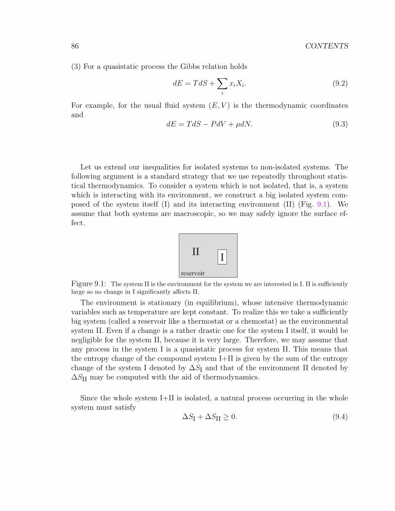
86 CONTENTS
(3) For a quasistatic process the Gibbs relation holds
dE = TdS +∑
i
xiXi. (9.2)
For example, for the usual fluid system (E, V ) is the thermodynamic coordinatesand
dE = TdS − PdV + µdN. (9.3)
Let us extend our inequalities for isolated systems to non-isolated systems. Thefollowing argument is a standard strategy that we use repeatedly throughout statis-tical thermodynamics. To consider a system which is not isolated, that is, a systemwhich is interacting with its environment, we construct a big isolated system com-posed of the system itself (I) and its interacting environment (II) (Fig. 9.1). Weassume that both systems are macroscopic, so we may safely ignore the surface ef-fect.
III
reservoir
Figure 9.1: The system II is the environment for the system we are interested in I. II is sufficientlylarge so no change in I significantly affects II.
The environment is stationary (in equilibrium), whose intensive thermodynamicvariables such as temperature are kept constant. To realize this we take a sufficientlybig system (called a reservoir like a thermostat or a chemostat) as the environmentalsystem II. Even if a change is a rather drastic one for the system I itself, it would benegligible for the system II, because it is very large. Therefore, we may assume thatany process in the system I is a quasistatic process for system II. This means thatthe entropy change of the compound system I+II is given by the sum of the entropychange of the system I denoted by ∆SI and that of the environment II denoted by∆SII may be computed with the aid of thermodynamics.
Since the whole system I+II is isolated, a natural process occurring in the wholesystem must satisfy
∆SI + ∆SII ≥ 0. (9.4)
9. LECTURE 9: THERMODYNAMICS: GENERAL CONSEQUENCES 87
Let Q (> 0) be the heat transferred to the system I from the environment II. Fromour assumption, we have
∆SII = −Q/Te, (9.5)
where Te is the temperature of the environment. The minus sign is because II islosing heat to I. Combining (9.4) and (9.5) yields the following inequality:
∆SI ≥ Q/Te. (9.6)
This is Clausius’ inequality for non-isolated systems. Of course, for isolated systemsQ vanishes, so we recover the isolated case.
If the change in I is reversible, then ∆SI = Q/Te should hold; (9.6) implies that‘excessive entropy’ has been produced in I by the irreversibility of the process.
Suppose an isolated system is in equilibrium initially. Then, some constraint inthe system (e.g., a wall inside) is removed, and the system reaches another equilib-rium eventually. Since the change is spontaneous, it must be an irreversible process(you go to another equilibrium, which will never change, so you can never returnto the original state). Therefore, entropy increases. This tells us that if there is aspontaneous change in thermodynamic states, entropy can further increase. There-fore, it s state is a stable equilibrium its entropy must be maximum under the givenconstraints; the initial state of the above process has the maximum entropy allowedto it under the old constraints. Only because the constraint is removed could theentropy of the system increase further.
Thus, we my conclude a variational principle (entropy maximization principle):the equilibrium state is characterized by the maximum entropy under the given con-straint of the system.
δS ≤ 0 (9.7)
if the state is in a stable equilibrium. Here, δ denotes (usually) virtual changes, butactually, thermal fluctuation is always making various changes and always checkingthis inequality spontaneously.
As an application of the entropy maximization principle, let us study the equilib-rium condition for two systems I and II interacting through various walls.
i) Consider a rigid impermeable wall which is diathermal. Thus, the two systems incontact through this wall exchange energy (internal energy) in the form of heat. Thetotal entropy of the system S is the sum of the entropy of each system SI and SII.The total internal energy E is also the sum of subsystem internal energies EI and EII(extensivity). We isolate the compound system and ask the equilibrium condition
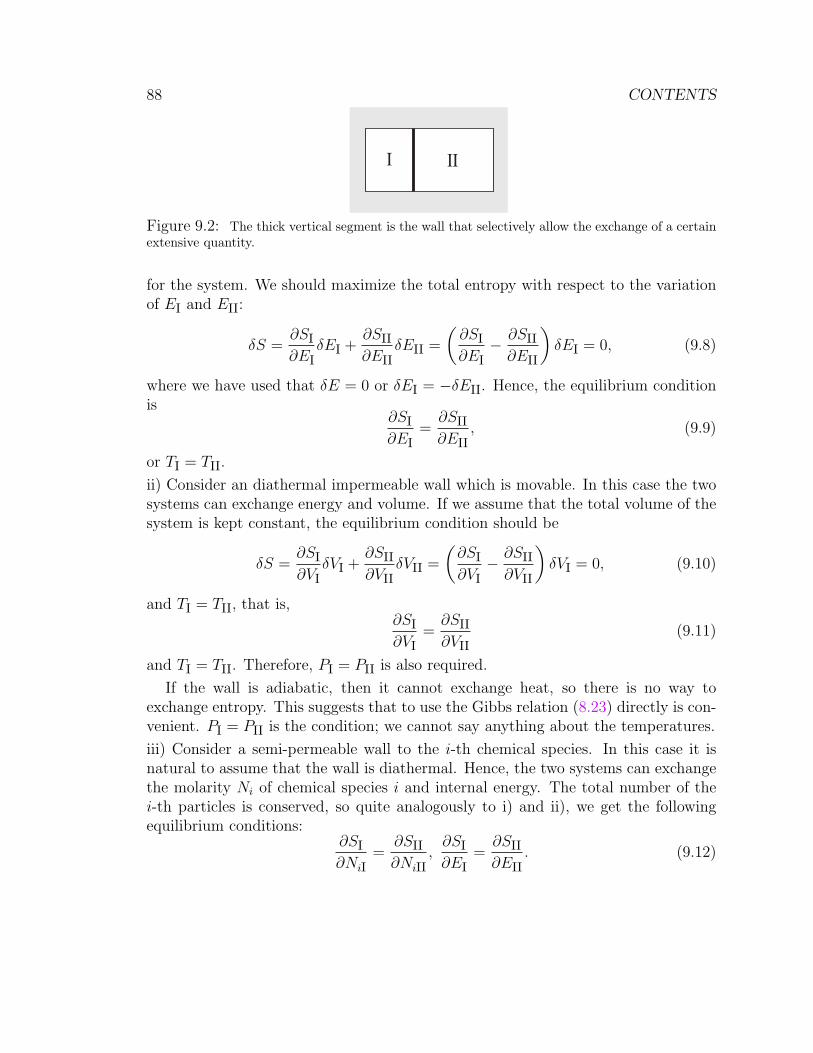
88 CONTENTS
I II
Figure 9.2: The thick vertical segment is the wall that selectively allow the exchange of a certainextensive quantity.
for the system. We should maximize the total entropy with respect to the variationof EI and EII:
δS =∂SI∂EI
δEI +∂SII∂EII
δEII =
(∂SI∂EI− ∂SII∂EII
)δEI = 0, (9.8)
where we have used that δE = 0 or δEI = −δEII. Hence, the equilibrium conditionis
∂SI∂EI
=∂SII∂EII
, (9.9)
or TI = TII.
ii) Consider an diathermal impermeable wall which is movable. In this case the twosystems can exchange energy and volume. If we assume that the total volume of thesystem is kept constant, the equilibrium condition should be
δS =∂SI∂VI
δVI +∂SII∂VII
δVII =
(∂SI∂VI− ∂SII∂VII
)δVI = 0, (9.10)
and TI = TII, that is,∂SI∂VI
=∂SII∂VII
(9.11)
and TI = TII. Therefore, PI = PII is also required.
If the wall is adiabatic, then it cannot exchange heat, so there is no way toexchange entropy. This suggests that to use the Gibbs relation (8.23) directly is con-venient. PI = PII is the condition; we cannot say anything about the temperatures.
iii) Consider a semi-permeable wall to the i-th chemical species. In this case it isnatural to assume that the wall is diathermal. Hence, the two systems can exchangethe molarity Ni of chemical species i and internal energy. The total number of thei-th particles is conserved, so quite analogously to i) and ii), we get the followingequilibrium conditions:
∂SI∂NiI
=∂SII∂NiII
,∂SI∂EI
=∂SII∂EII
. (9.12)
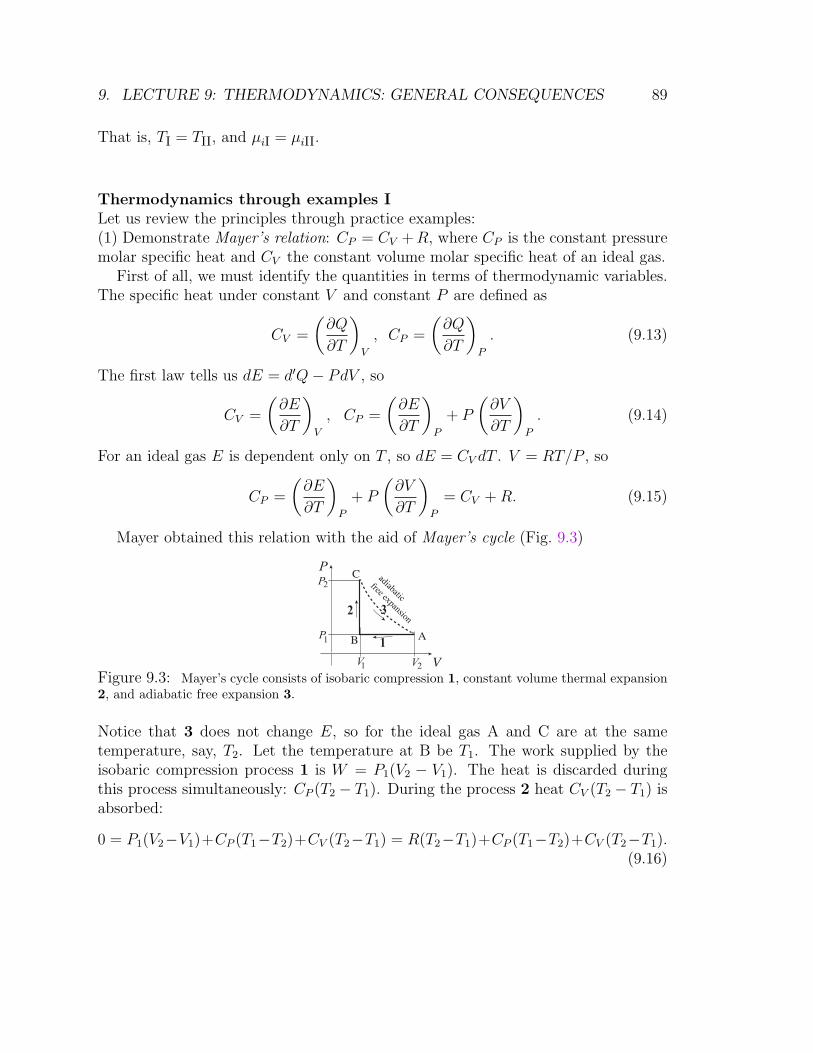
9. LECTURE 9: THERMODYNAMICS: GENERAL CONSEQUENCES 89
That is, TI = TII, and µiI = µiII.
Thermodynamics through examples ILet us review the principles through practice examples:(1) Demonstrate Mayer’s relation: CP = CV +R, where CP is the constant pressuremolar specific heat and CV the constant volume molar specific heat of an ideal gas.
First of all, we must identify the quantities in terms of thermodynamic variables.The specific heat under constant V and constant P are defined as
CV =
(∂Q
∂T
)V
, CP =
(∂Q
∂T
)P
. (9.13)
The first law tells us dE = d′Q− PdV , so
CV =
(∂E
∂T
)V
, CP =
(∂E
∂T
)P
+ P
(∂V
∂T
)P
. (9.14)
For an ideal gas E is dependent only on T , so dE = CV dT . V = RT/P , so
CP =
(∂E
∂T
)P
+ P
(∂V
∂T
)P
= CV +R. (9.15)
Mayer obtained this relation with the aid of Mayer’s cycle (Fig. 9.3)
adiabatic
free expansion
V
P
P
VV
P2
1
1 2
1
2 3
AB
C
Figure 9.3: Mayer’s cycle consists of isobaric compression 1, constant volume thermal expansion2, and adiabatic free expansion 3.
Notice that 3 does not change E, so for the ideal gas A and C are at the sametemperature, say, T2. Let the temperature at B be T1. The work supplied by theisobaric compression process 1 is W = P1(V2 − V1). The heat is discarded duringthis process simultaneously: CP (T2 − T1). During the process 2 heat CV (T2 − T1) isabsorbed:
0 = P1(V2−V1)+CP (T1−T2)+CV (T2−T1) = R(T2−T1)+CP (T1−T2)+CV (T2−T1).(9.16)
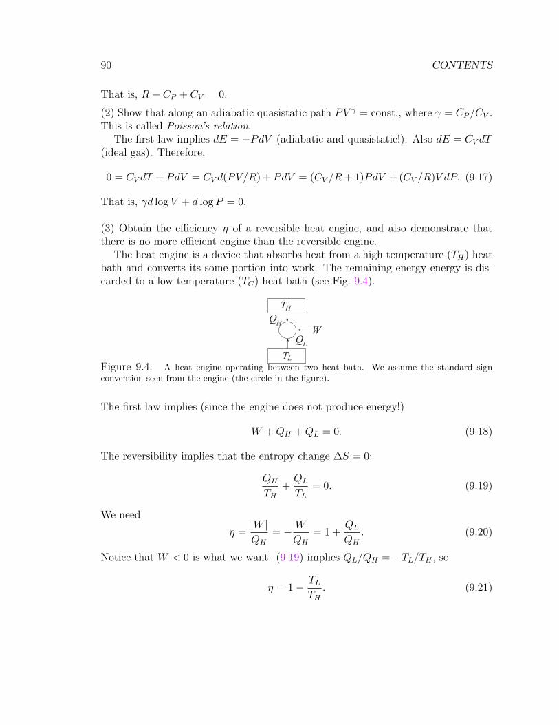
90 CONTENTS
That is, R− CP + CV = 0.
(2) Show that along an adiabatic quasistatic path PV γ = const., where γ = CP/CV .This is called Poisson’s relation.
The first law implies dE = −PdV (adiabatic and quasistatic!). Also dE = CV dT(ideal gas). Therefore,
0 = CV dT +PdV = CV d(PV/R) +PdV = (CV /R+ 1)PdV + (CV /R)V dP. (9.17)
That is, γd log V + d logP = 0.
(3) Obtain the efficiency η of a reversible heat engine, and also demonstrate thatthere is no more efficient engine than the reversible engine.
The heat engine is a device that absorbs heat from a high temperature (TH) heatbath and converts its some portion into work. The remaining energy energy is dis-carded to a low temperature (TC) heat bath (see Fig. 9.4).
Q
QW
T
TL
H
H
L
Figure 9.4: A heat engine operating between two heat bath. We assume the standard signconvention seen from the engine (the circle in the figure).
The first law implies (since the engine does not produce energy!)
W +QH +QL = 0. (9.18)
The reversibility implies that the entropy change ∆S = 0:
QH
TH
+QL
TL
= 0. (9.19)
We need
η =|W |QH
= − W
QH
= 1 +QL
QH
. (9.20)
Notice that W < 0 is what we want. (9.19) implies QL/QH = −TL/TH , so
η = 1− TL
TH
. (9.21)
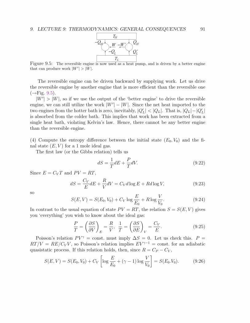
9. LECTURE 9: THERMODYNAMICS: GENERAL CONSEQUENCES 91
−Q
−Q
W
T
TL
H
H
L
Q
Q’
−W’ H
L
Figure 9.5: The reversible engine is now used as a heat pump, and is driven by a better enginethat can produce work |W ′| > |W |.
The reversible engine can be driven backward by supplying work. Let us drivethe reversible engine by another engine that is more efficient than the reversible one(→Fig. 9.5).|W ′| > |W |, so if we use the output of the ‘better engine’ to drive the reversible
engine, we can still utilize the work |W ′| − |W |. Since the net heat imported to thetwo engines from the hotter bath is zero, inevitably, |Q′
L| < |QL|. That is, |QL|−|Q′L|
is absorbed from the colder bath. This implies that work has been extracted from asingle heat bath, violating Kelvin’s law. Hence, there cannot be any better enginethan the reversible engine.
(4) Compute the entropy difference between the initial state (E0, V0) and the fi-nal state (E, V ) for a 1 mole ideal gas.
The first law (or the Gibbs relation) tells us
dS =1
TdE +
P
TdV. (9.22)
Since E = CV T and PV = RT ,
dS =CV
EdE +
R
VdV = CV d logE +Rd log V, (9.23)
so
S(E, V ) = S(E0, V0) + CV logE
E0
+R logV
V0
. (9.24)
In contrast to the usual equation of state PV = RT , the relation S = S(E, V ) givesyou ‘everything’ you wish to know about the ideal gas:
P
T=
(∂S
∂V
)E
=R
V,
1
T=
(∂S
∂E
)V
=CV
E. (9.25)
Poisson’s relation PV γ = const. must imply ∆S = 0. Let us check this. P =RT/V = RE/CV V , so Poisson’s relation implies EV γ−1 = const. for an adiabaticquasistatic process. If this relation holds, then, since R = CP − CV ,
S(E, V ) = S(E0, V0) + CV
[log
E
E0
+ (γ − 1) logV
V0
]= S(E0.V0). (9.26)

92 CONTENTS
That is, the entropy does not change as expected. Of course, we used this relationto derive Poisson’s relation, so there is no surprise at all.
(5) There are two blocks with the same heat capacity at T1 and at T2, respec-tively. We can operate a reversible engine between these two block until they exhibitthe same temperature. What is the final temperature? How much work can youobtain?
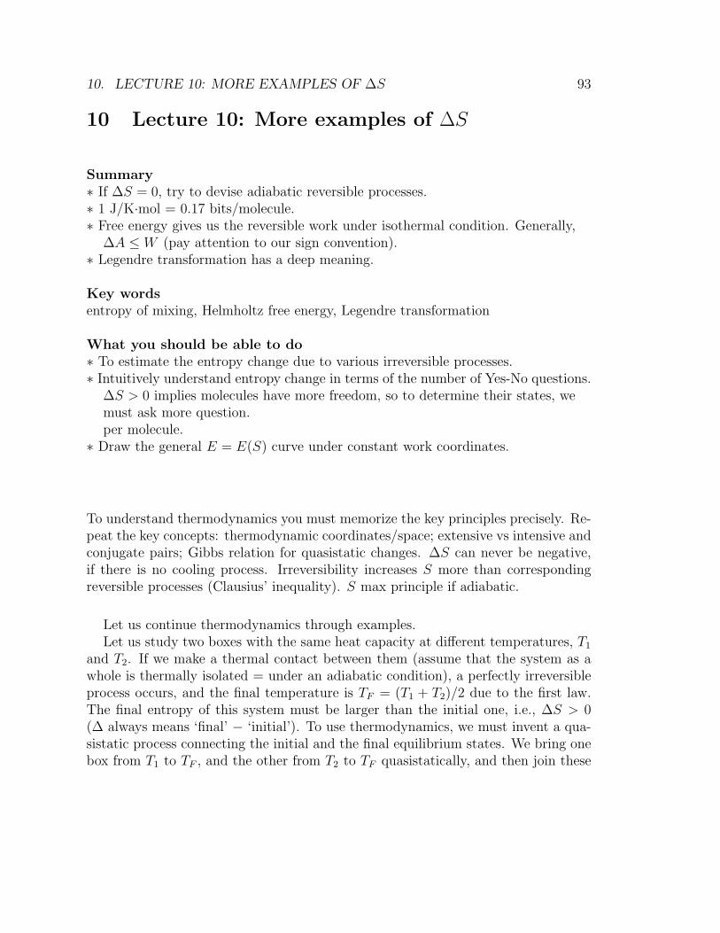
10. LECTURE 10: MORE EXAMPLES OF ∆S 93
10 Lecture 10: More examples of ∆S
Summary∗ If ∆S = 0, try to devise adiabatic reversible processes.∗ 1 J/K·mol = 0.17 bits/molecule.∗ Free energy gives us the reversible work under isothermal condition. Generally,
∆A ≤ W (pay attention to our sign convention).∗ Legendre transformation has a deep meaning.
Key wordsentropy of mixing, Helmholtz free energy, Legendre transformation
What you should be able to do∗ To estimate the entropy change due to various irreversible processes.∗ Intuitively understand entropy change in terms of the number of Yes-No questions.
∆S > 0 implies molecules have more freedom, so to determine their states, wemust ask more question.per molecule.
∗ Draw the general E = E(S) curve under constant work coordinates.
To understand thermodynamics you must memorize the key principles precisely. Re-peat the key concepts: thermodynamic coordinates/space; extensive vs intensive andconjugate pairs; Gibbs relation for quasistatic changes. ∆S can never be negative,if there is no cooling process. Irreversibility increases S more than correspondingreversible processes (Clausius’ inequality). S max principle if adiabatic.
Let us continue thermodynamics through examples.Let us study two boxes with the same heat capacity at different temperatures, T1
and T2. If we make a thermal contact between them (assume that the system as awhole is thermally isolated = under an adiabatic condition), a perfectly irreversibleprocess occurs, and the final temperature is TF = (T1 + T2)/2 due to the first law.The final entropy of this system must be larger than the initial one, i.e., ∆S > 0(∆ always means ‘final’ − ‘initial’). To use thermodynamics, we must invent a qua-sistatic process connecting the initial and the final equilibrium states. We bring onebox from T1 to TF , and the other from T2 to TF quasistatically, and then join these
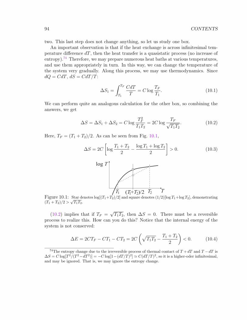
94 CONTENTS
two. This last step does not change anything, so let us study one box.An important observation is that if the heat exchange is across infinitesimal tem-
perature difference dT , then the heat transfer is a quasistatic process (no increase ofentropy).74 Therefore, we may prepare numerous heat baths at various temperatures,and use them appropriately in turn. In this way, we can change the temperature ofthe system very gradually. Along this process, we may use thermodynamics. SincedQ = CdT , dS = CdT/T :
∆S1 =
∫ TF
T1
CdT
T= C log
TF
T1
. (10.1)
We can perform quite an analogous calculation for the other box, so combining theanswers, we get
∆S = ∆S1 + ∆S2 = C logT 2
F
T1T2
= 2C logTF√T1T2
. (10.2)
Here, TF = (T1 + T2)/2. As can be seen from Fig. 10.1,
∆S = 2C
[log
T1 + T2
2− log T1 + log T2
2
]> 0. (10.3)
log T
TTT1 2(T+ )/2 T21Figure 10.1: Star denotes log[(T1+T2)/2] and square denotes (1/2)[log T1+log T2], demonstrating(T1 + T2)/2 >
√T1T2.
(10.2) implies that if TF =√T1T2, then ∆S = 0. There must be a reversible
process to realize this. How can you do this? Notice that the internal energy of thesystem is not conserved:
∆E = 2CTF − CT1 − CT2 = 2C
(√T1T2 −
T1 + T2
2
)< 0. (10.4)
74The entropy change due to the irreversible process of thermal contact of T + dT and T − dT is∆S = C log[T 2/(T 2−dT 2)] = −C log[1−(dT/T )2] ' C(dT/T )2, so it is a higher-oder infinitesimal,and may be ignored. That is, we may ignore the entropy change.
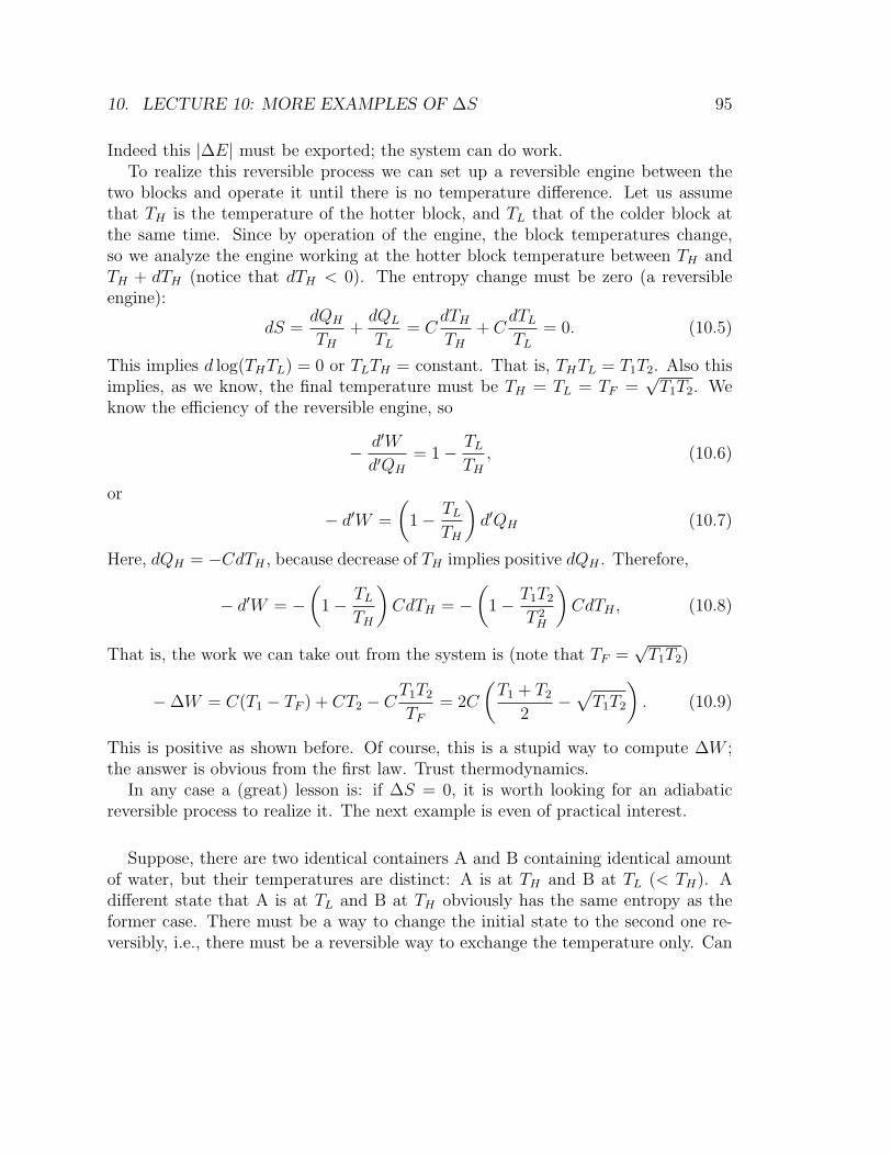
10. LECTURE 10: MORE EXAMPLES OF ∆S 95
Indeed this |∆E| must be exported; the system can do work.To realize this reversible process we can set up a reversible engine between the
two blocks and operate it until there is no temperature difference. Let us assumethat TH is the temperature of the hotter block, and TL that of the colder block atthe same time. Since by operation of the engine, the block temperatures change,so we analyze the engine working at the hotter block temperature between TH andTH + dTH (notice that dTH < 0). The entropy change must be zero (a reversibleengine):
dS =dQH
TH
+dQL
TL
= CdTH
TH
+ CdTL
TL
= 0. (10.5)
This implies d log(THTL) = 0 or TLTH = constant. That is, THTL = T1T2. Also thisimplies, as we know, the final temperature must be TH = TL = TF =
√T1T2. We
know the efficiency of the reversible engine, so
− d′W
d′QH
= 1− TL
TH
, (10.6)
or
− d′W =
(1− TL
TH
)d′QH (10.7)
Here, dQH = −CdTH , because decrease of TH implies positive dQH . Therefore,
− d′W = −(
1− TL
TH
)CdTH = −
(1− T1T2
T 2H
)CdTH , (10.8)
That is, the work we can take out from the system is (note that TF =√T1T2)
−∆W = C(T1 − TF ) + CT2 − CT1T2
TF
= 2C
(T1 + T2
2−√T1T2
). (10.9)
This is positive as shown before. Of course, this is a stupid way to compute ∆W ;the answer is obvious from the first law. Trust thermodynamics.
In any case a (great) lesson is: if ∆S = 0, it is worth looking for an adiabaticreversible process to realize it. The next example is even of practical interest.
Suppose, there are two identical containers A and B containing identical amountof water, but their temperatures are distinct: A is at TH and B at TL (< TH). Adifferent state that A is at TL and B at TH obviously has the same entropy as theformer case. There must be a way to change the initial state to the second one re-versibly, i.e., there must be a reversible way to exchange the temperature only. Can
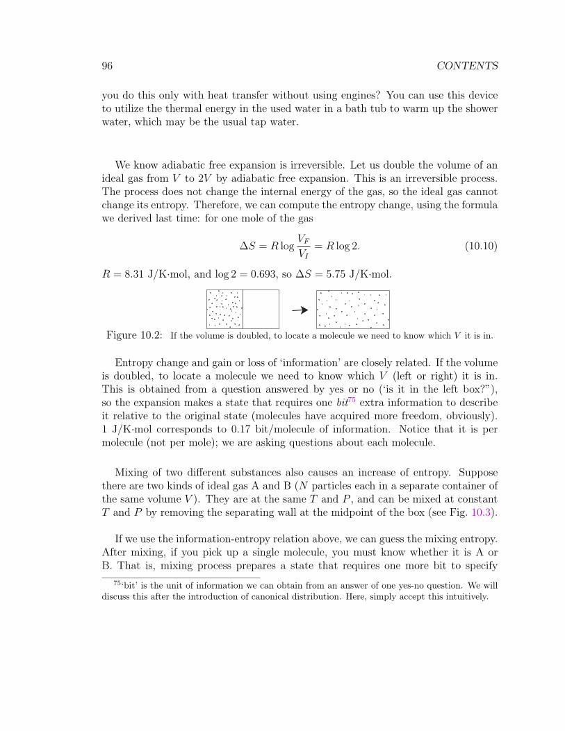
96 CONTENTS
you do this only with heat transfer without using engines? You can use this deviceto utilize the thermal energy in the used water in a bath tub to warm up the showerwater, which may be the usual tap water.
We know adiabatic free expansion is irreversible. Let us double the volume of anideal gas from V to 2V by adiabatic free expansion. This is an irreversible process.The process does not change the internal energy of the gas, so the ideal gas cannotchange its entropy. Therefore, we can compute the entropy change, using the formulawe derived last time: for one mole of the gas
∆S = R logVF
VI
= R log 2. (10.10)
R = 8.31 J/K·mol, and log 2 = 0.693, so ∆S = 5.75 J/K·mol.
Figure 10.2: If the volume is doubled, to locate a molecule we need to know which V it is in.
Entropy change and gain or loss of ‘information’ are closely related. If the volumeis doubled, to locate a molecule we need to know which V (left or right) it is in.This is obtained from a question answered by yes or no (‘is it in the left box?”),so the expansion makes a state that requires one bit75 extra information to describeit relative to the original state (molecules have acquired more freedom, obviously).1 J/K·mol corresponds to 0.17 bit/molecule of information. Notice that it is permolecule (not per mole); we are asking questions about each molecule.
Mixing of two different substances also causes an increase of entropy. Supposethere are two kinds of ideal gas A and B (N particles each in a separate container ofthe same volume V ). They are at the same T and P , and can be mixed at constantT and P by removing the separating wall at the midpoint of the box (see Fig. 10.3).
If we use the information-entropy relation above, we can guess the mixing entropy.After mixing, if you pick up a single molecule, you must know whether it is A orB. That is, mixing process prepares a state that requires one more bit to specify
75‘bit’ is the unit of information we can obtain from an answer of one yes-no question. We willdiscuss this after the introduction of canonical distribution. Here, simply accept this intuitively.
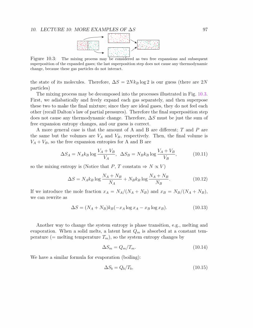
10. LECTURE 10: MORE EXAMPLES OF ∆S 97
Figure 10.3: The mixing process may be considered as two free expansions and subsequentsuperposition of the expanded gases; the last superposition step does not cause any thermodynamicchange, because these gas particles do not interact.
the state of its molecules. Therefore, ∆S = 2NkB log 2 is our guess (there are 2Nparticles)
The mixing process may be decomposed into the processes illustrated in Fig. 10.3.First, we adiabatically and freely expand each gas separately, and then superposethese two to make the final mixture; since they are ideal gases, they do not feel eachother (recall Dalton’s law of partial pressures). Therefore the final superposition stepdoes not cause any thermodynamic change. Therefore, ∆S must be just the sum offree expansion entropy changes, and our guess is correct.
A more general case is that the amount of A and B are different; T and P arethe same but the volumes are VA and VB, respectively. Then, the final volume isVA + VB, so the free expansion entropies for A and B are
∆SA = NAkB logVA + VB
VA
, ∆SB = NBkB logVA + VB
VB
, (10.11)
so the mixing entropy is (Notice that P , T constatn ⇒ N ∝ V )
∆S = NAkB logNA +NB
NA
+NBkB logNA +NB
NB
. (10.12)
If we introduce the mole fraction xA = NA/(NA + NB) and xB = NB/(NA + NB),we can rewrite as
∆S = (NA +NB)kB(−xA log xA − xB log xB). (10.13)
Another way to change the system entropy is phase transition, e.g., melting andevaporation. When a solid melts, a latent heat Qm is absorbed at a constant tem-perature (= melting temperature Tm), so the system entropy changes by
∆Sm = Qm/Tm. (10.14)
We have a similar formula for evaporation (boiling):
∆Sb = Qb/Tb, (10.15)
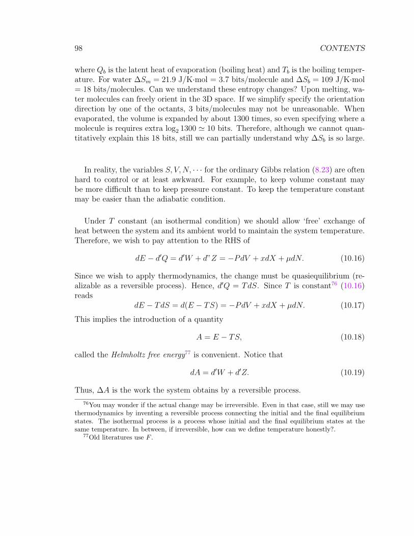
98 CONTENTS
where Qb is the latent heat of evaporation (boiling heat) and Tb is the boiling temper-ature. For water ∆Sm = 21.9 J/K·mol = 3.7 bits/molecule and ∆Sb = 109 J/K·mol= 18 bits/molecules. Can we understand these entropy changes? Upon melting, wa-ter molecules can freely orient in the 3D space. If we simplify specify the orientationdirection by one of the octants, 3 bits/molecules may not be unreasonable. Whenevaporated, the volume is expanded by about 1300 times, so even specifying where amolecule is requires extra log2 1300 ' 10 bits. Therefore, although we cannot quan-titatively explain this 18 bits, still we can partially understand why ∆Sb is so large.
In reality, the variables S, V,N, · · · for the ordinary Gibbs relation (8.23) are oftenhard to control or at least awkward. For example, to keep volume constant maybe more difficult than to keep pressure constant. To keep the temperature constantmay be easier than the adiabatic condition.
Under T constant (an isothermal condition) we should allow ‘free’ exchange ofheat between the system and its ambient world to maintain the system temperature.Therefore, we wish to pay attention to the RHS of
dE − d′Q = d′W + d”Z = −PdV + xdX + µdN. (10.16)
Since we wish to apply thermodynamics, the change must be quasiequilibrium (re-alizable as a reversible process). Hence, d′Q = TdS. Since T is constant76 (10.16)reads
dE − TdS = d(E − TS) = −PdV + xdX + µdN. (10.17)
This implies the introduction of a quantity
A = E − TS, (10.18)
called the Helmholtz free energy77 is convenient. Notice that
dA = d′W + d′Z. (10.19)
Thus, ∆A is the work the system obtains by a reversible process.
76You may wonder if the actual change may be irreversible. Even in that case, still we may usethermodynamics by inventing a reversible process connecting the initial and the final equilibriumstates. The isothermal process is a process whose initial and the final equilibrium states at thesame temperature. In between, if irreversible, how can we define temperature honestly?.
77Old literatures use F .
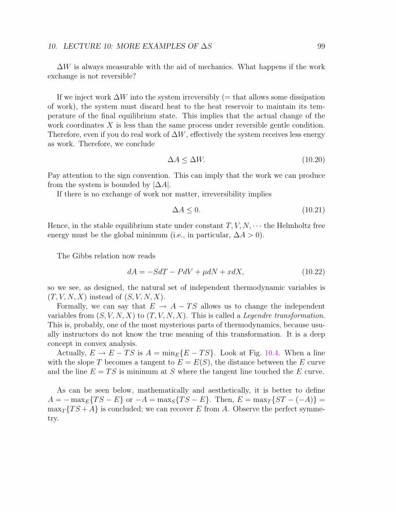
10. LECTURE 10: MORE EXAMPLES OF ∆S 99
∆W is always measurable with the aid of mechanics. What happens if the workexchange is not reversible?
If we inject work ∆W into the system irreversibly (= that allows some dissipationof work), the system must discard heat to the heat reservoir to maintain its tem-perature of the final equilibrium state. This implies that the actual change of thework coordinates X is less than the same process under reversible gentle condition.Therefore, even if you do real work of ∆W , effectively the system receives less energyas work. Therefore, we conclude
∆A ≤ ∆W. (10.20)
Pay attention to the sign convention. This can imply that the work we can producefrom the system is bounded by |∆A|.
If there is no exchange of work nor matter, irreversibility implies
∆A ≤ 0. (10.21)
Hence, in the stable equilibrium state under constant T, V,N, · · · the Helmholtz freeenergy must be the global minimum (i.e., in particular, ∆A > 0).
The Gibbs relation now reads
dA = −SdT − PdV + µdN + xdX, (10.22)
so we see, as designed, the natural set of independent thermodynamic variables is(T, V,N,X) instead of (S, V,N,X).
Formally, we can say that E → A − TS allows us to change the independentvariables from (S, V,N,X) to (T, V,N,X). This is called a Legendre transformation.This is, probably, one of the most mysterious parts of thermodynamics, because usu-ally instructors do not know the true meaning of this transformation. It is a deepconcept in convex analysis.
Actually, E → E − TS is A = minEE − TS. Look at Fig. 10.4. When a linewith the slope T becomes a tangent to E = E(S), the distance between the E curveand the line E = TS is minimum at S where the tangent line touched the E curve.
As can be seen below, mathematically and aesthetically, it is better to defineA = −maxETS − E or −A = maxSTS − E. Then, E = maxTST − (−A) =maxTTS+A is concluded; we can recover E from A. Observe the perfect symme-try.
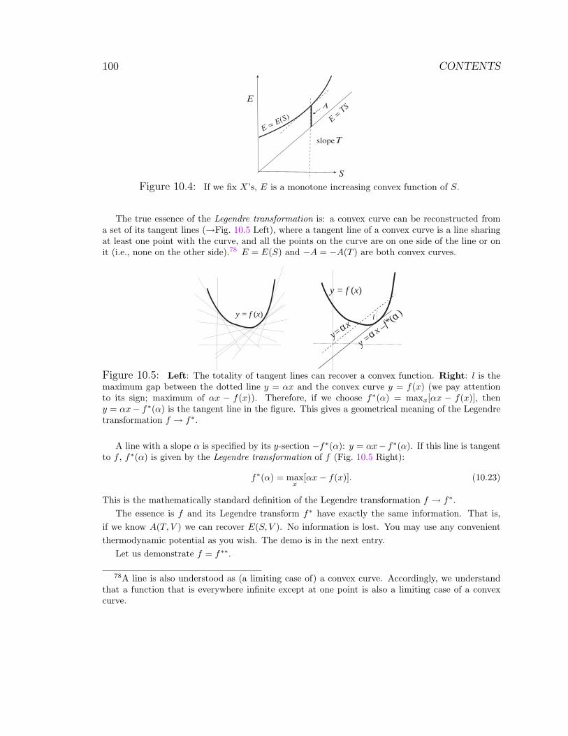
100 CONTENTS
E
S
Tslope
E = T
S
E = E(S)
A
Figure 10.4: If we fix X’s, E is a monotone increasing convex function of S.
The true essence of the Legendre transformation is: a convex curve can be reconstructed froma set of its tangent lines (→Fig. 10.5 Left), where a tangent line of a convex curve is a line sharingat least one point with the curve, and all the points on the curve are on one side of the line or onit (i.e., none on the other side).78 E = E(S) and −A = −A(T ) are both convex curves.
y = f (x)
y= xα
y = x
f*(
)α
α _
l
y = f (x)
Figure 10.5: Left: The totality of tangent lines can recover a convex function. Right: l is themaximum gap between the dotted line y = αx and the convex curve y = f(x) (we pay attentionto its sign; maximum of αx − f(x)). Therefore, if we choose f∗(α) = maxx[αx − f(x)], theny = αx− f∗(α) is the tangent line in the figure. This gives a geometrical meaning of the Legendretransformation f → f∗.
A line with a slope α is specified by its y-section −f∗(α): y = αx− f∗(α). If this line is tangentto f , f∗(α) is given by the Legendre transformation of f (Fig. 10.5 Right):
f∗(α) = maxx
[αx− f(x)]. (10.23)
This is the mathematically standard definition of the Legendre transformation f → f∗.The essence is f and its Legendre transform f∗ have exactly the same information. That is,
if we know A(T, V ) we can recover E(S, V ). No information is lost. You may use any convenientthermodynamic potential as you wish. The demo is in the next entry.
Let us demonstrate f = f∗∗.
78A line is also understood as (a limiting case of) a convex curve. Accordingly, we understandthat a function that is everywhere infinite except at one point is also a limiting case of a convexcurve.
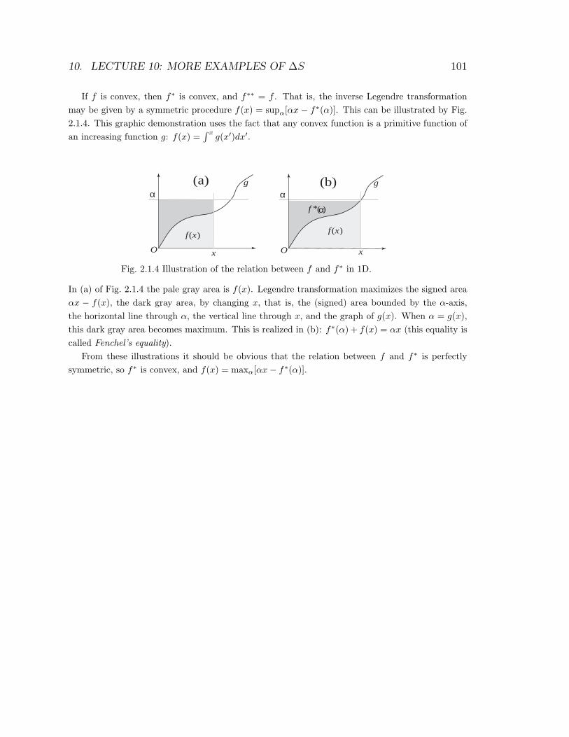
10. LECTURE 10: MORE EXAMPLES OF ∆S 101
If f is convex, then f∗ is convex, and f∗∗ = f . That is, the inverse Legendre transformationmay be given by a symmetric procedure f(x) = supα[αx− f∗(α)]. This can be illustrated by Fig.2.1.4. This graphic demonstration uses the fact that any convex function is a primitive function ofan increasing function g: f(x) =
∫ xg(x′)dx′.
α
x
g
O
( )xf
α
x
g
O
( )xf
( )f * α
(b)(a)
Fig. 2.1.4 Illustration of the relation between f and f∗ in 1D.
In (a) of Fig. 2.1.4 the pale gray area is f(x). Legendre transformation maximizes the signed areaαx − f(x), the dark gray area, by changing x, that is, the (signed) area bounded by the α-axis,the horizontal line through α, the vertical line through x, and the graph of g(x). When α = g(x),this dark gray area becomes maximum. This is realized in (b): f∗(α) + f(x) = αx (this equality iscalled Fenchel’s equality).
From these illustrations it should be obvious that the relation between f and f∗ is perfectlysymmetric, so f∗ is convex, and f(x) = maxα[αx− f∗(α)].
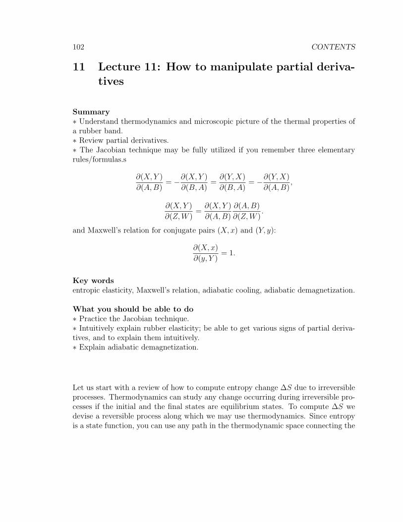
102 CONTENTS
11 Lecture 11: How to manipulate partial deriva-
tives
Summary∗ Understand thermodynamics and microscopic picture of the thermal properties ofa rubber band.∗ Review partial derivatives.∗ The Jacobian technique may be fully utilized if you remember three elementaryrules/formulas.s
∂(X, Y )
∂(A,B)= −∂(X, Y )
∂(B,A)=∂(Y,X)
∂(B,A)= −∂(Y,X)
∂(A,B),
∂(X, Y )
∂(Z,W )=∂(X, Y )
∂(A,B)
∂(A,B)
∂(Z,W ).
and Maxwell’s relation for conjugate pairs (X, x) and (Y, y):
∂(X, x)
∂(y, Y )= 1.
Key wordsentropic elasticity, Maxwell’s relation, adiabatic cooling, adiabatic demagnetization.
What you should be able to do∗ Practice the Jacobian technique.∗ Intuitively explain rubber elasticity; be able to get various signs of partial deriva-tives, and to explain them intuitively.∗ Explain adiabatic demagnetization.
Let us start with a review of how to compute entropy change ∆S due to irreversibleprocesses. Thermodynamics can study any change occurring during irreversible pro-cesses if the initial and the final states are equilibrium states. To compute ∆S wedevise a reversible process along which we may use thermodynamics. Since entropyis a state function, you can use any path in the thermodynamic space connecting the

11. LECTURE 11: HOW TO MANIPULATE PARTIAL DERIVATIVES 103
initial and the final states. For example, if T and P are given as functions of E andV , we can integrate
dS =1
TdE +
P
TdV (11.1)
along a convenient path connecting the initial and the final states (Fig. 11.1).
S
E
V
actual
irreversible process
S =S(E,V)
Figure 11.1: You can integrate the Gibbs relation (11.1) along any path in the (E, V ) space (i.e.,the thermodynamic space), because S is a state function, BUT there are convenient paths such asare piecewise parallel to thermodynamic coordinates (red path).
Let us perform a small experiment of quasistatic adiabatic processes using a rubberband. Prepare a thick rubber band (that is used to bundle, e.g., asparagus). Useyour lip as a temperature sensor. Initially, putting the rubber band to your lip, yousense the room temperature (cool). Now, you hold a small portion of the band byyour hands and stretch it tightly and quickly. Then, feel its temperature with yourlip. It must be warm. You have just demonstrated(
∂T
∂L
)S
> 0, (11.2)
where L is the length of the stretched portion of the rubber band. The Gibbs relationfor a rubber band reads
dE = TdS + FdL, (11.3)
where F is force stretching the band. Since the process is adiabatic and quasistaticS is constant. Even if you rapidly pull the band, the process is very slow from the
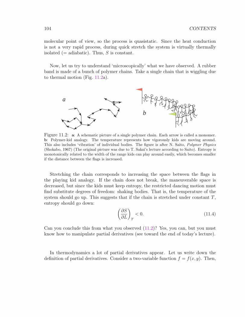
104 CONTENTS
molecular point of view, so the process is quasistatic. Since the heat conductionis not a very rapid process, during quick stretch the system is virtually thermallyisolated (= adiabatic). Thus, S is constant.
Now, let us try to understand ‘microscopically’ what we have observed. A rubberband is made of a bunch of polymer chains. Take a single chain that is wiggling dueto thermal motion (Fig. 11.2a).
a
b
Figure 11.2: a: A schematic picture of a single polymer chain. Each arrow is called a monomer.b: Polymer-kid analogy. The temperature represents how vigorously kids are moving around.This also includes ‘vibration’ of individual bodies. The figure is after N. Saito, Polymer Physics(Shokabo, 1967) (The original picture was due to T. Sakai’s lecture according to Saito). Entropy ismonotonically related to the width of the range kids can play around easily, which becomes smallerif the distance between the flags is increased.
Stretching the chain corresponds to increasing the space between the flags inthe playing kid analogy. If the chain does not break, the maneuverable space isdecreased, but since the kids must keep entropy, the restricted dancing motion mustfind substitute degrees of freedom: shaking bodies. That is, the temperature of thesystem should go up. This suggests that if the chain is stretched under constant T ,entropy should go down: (
∂S
∂L
)T
< 0. (11.4)
Can you conclude this from what you observed (11.2)? Yes, you can, but you mustknow how to manipulate partial derivatives (see toward the end of today’s lecture).
In thermodynamics a lot of partial derivatives appear. Let us write down thedefinition of partial derivatives. Consider a two-variable function f = f(x, y). Then,
11. LECTURE 11: HOW TO MANIPULATE PARTIAL DERIVATIVES 105
partial derivatives are defined as
∂f
∂x≡ fx = lim
δx→0
f(x+ δx, y)− f(x, y)
δx, (11.5)
∂f
∂y≡ fy = lim
δy→0
f(x, y + δy)− f(x, y)
δy. (11.6)
Partial differentiation is extremely tricky in general. For example, even if ∂f/∂xand ∂f/∂y exist at a point, f can be discontinuous at the same point. E is oncecontinuously differentiable with respect to S and work coordinates, so we may studyfairly well-behaved functions.
Let f be a function of several variables x = (x1, · · · , xn). We could understand fas a function of the vector x. We wish to study its ‘linear response to the changex→ x + δx:
δf(x) = f(x + δx)− f(x) = Df(x)dx + o[δx], (11.7)
where o denotes higher order terms that vanishes faster than ‖δx‖, when the limitδx→ 0 is taken. Here, Df is a linear operator79 that can be written as
Df(x)dx =∑
i
∂f
∂xi
dxi (11.8)
If such a linear map Df is well-defined, we say that f is (totally) differentiable. Ifthere are only two variables,
Df(x, y)(dx, dy) =∂f
∂xdx+
∂f
∂ydy. (11.9)
Consider f(x + δx, y + δy) − f(x, y). There are two ways to go from (x, y) to(x+ δx, y + δy), δx first or δy first:
f(x+ δx, y + δy)− f(x, y) = f(x+ δx, y + δy)− f(x+ δx, y) + f(x+ δx, y)− f(x, y)
= fy(x+ δx, y)dy + fx(x, y)dx, (11.10)
f(x+ δx, y + δy)− f(x, y) = f(x+ δx, y + δy)− f(x, y + δy) + f(x, y + δy)− f(x, y)
= fx(x, y + δy)dx+ fy(x, y)dy. (11.11)
79L is a linear operator acting on a function set F is a map from F to some other vector spacesuch that
L(αf + βg) = αLf + βLg
where f, g ∈ F and α, β are numbers.

106 CONTENTS
The difference of these two formulas is
[fy(x+ δx, y)− fy(x, y)]dy− [fx(x, y+ δy)− fx(x, y)]dx = [fxy(x, y)− fyx(x, y)]dxdy.(11.12)
This must vanish if the surface defined by f is at least twice differentiable.80 Thatis,
fxy = fyx. (11.13)
For example, for a rubber band dE = TdS + FdL, so(∂T
∂L
)S
=
(∂F
∂S
)L
. (11.14)
Such relations are called Maxwell’s relations.
To manipulate many partial derivatives, it is very convenient to use the so-calledJacobian technique. This technique may not even be taught in graduate courses,but it is easy to memorize, and easy to use. It can greatly reduce the insight andskill required in thermodynamics, especially with the Jacobian version of Maxwell’srelation (11.30).
The Jacobian for two independent variables is defined as the following determi-nant:
∂(X, Y )
∂(x, y)≡
∣∣∣∣∣∣(
∂X∂x
)y
(∂X∂y
)x(
∂Y∂x
)y
(∂Y∂y
)x
∣∣∣∣∣∣ =
(∂X
∂x
)y
(∂Y
∂y
)x
−(∂Y
∂x
)y
(∂X
∂y
)x
. (11.15)
In particular, we observe∂(X, y)
∂(x, y)=
(∂X
∂x
)y
, (11.16)
which is probably the key observation of this technique. Obviously,
∂(X, Y )
∂(X, Y )= 1. (11.17)
80We must say something more careful mathematically, but let us be contented with this fornow.
11. LECTURE 11: HOW TO MANIPULATE PARTIAL DERIVATIVES 107
There are only two or three formulas you should learn by heart (they are very easyto memorize). One is straightforwardly obtained from the definition of determinants:exchanging rows or columns switch the sign:
∂(X, Y )
∂(x, y)= −∂(X, Y )
∂(y, x)=∂(Y,X)
∂(y, x)= −∂(Y,X)
∂(x, y). (11.18)
If we assume that X and Y are functions of a and b, and that a and b are, in turn,functions of x and y, we have the following multiplicative relation:
∂(X, Y )
∂(a, b)
∂(a, b)
∂(x, y)=∂(X, Y )
∂(x, y). (11.19)
This is a disguised chain rule:(∂X
∂x
)y
=
(∂X
∂a
)b
(∂a
∂x
)y
+
(∂X
∂b
)a
(∂b
∂x
)y
, (11.20)
etc. Confirm (11.19) by yourself (use det(AB) = (detA)(detB)).The technical significance of (11.19) must be obvious; calculus becomes algebra:
you can think ∂(A,B) just as an ordinary numbers: formally we can do81
∂(X, Y )
∂(x, y)=∂(X, Y )
∂(x, y)
∂(A,B)
∂(A,B)=∂(X, Y )
∂(A,B)
∂(A,B)
∂(x, y). (11.21)
From (11.19) we get at once
∂(X, Y )
∂A,B)= 1
/∂(A,B)
∂(X, Y ). (11.22)
In particular, we have (∂X
∂x
)Y
= 1
/(∂x
∂X
)Y
. (11.23)
Examples: For a rubber band(∂L
∂S
)F
=∂(L, F )
∂(S, F )=∂(L, F )
∂(T, F )
∂(T, F )
∂(S, F )=
(∂L
∂T
)F
(∂T
∂S
)F
, (11.24)
81That is, all the derivatives showing up in the calculation are well defined. However, in practicalthermodynamics, you can be maximally formal.
108 CONTENTS
which reads (∂L
∂S
)F
=
(∂L
∂T
)F
/(∂S
∂T
)F
= T
(∂L
∂T
)F
/CF . (11.25)
Here, CF is the heat capacity under constant force. It is explained as follows: Thefirst law tells us d′Q = TdS, so if we differentiate this with respect to T underconstant F , it must be the heat capacity under constant F . Generally speaking, theheat capacity under constant X always have the following expression:
CX = T
(∂S
∂T
)X
. (11.26)
We will learn the consequence of the stability of the equilibrium states later, but thestability of the equilibrium state implies CX ≥ 0 (usually strictly positive). Imaginethe contrary. If you inject heat into a system, its temperature goes down, so it sucksmore heat from the surrounding world, and further reduces its temperature. Thatis, such a system becomes a bottomless heat sink.
Using these relations, we can easily demonstrate(∂X
∂y
)x
= −(∂x
∂y
)X
/(∂x
∂X
)y
(11.27)
as follows:
∂(X, x)
∂(y, x)
(11.19)=
∂(y,X)
∂(y, x)
∂(X, x)
∂(y,X)
(11.18)= −∂(x,X)
∂(y,X)
∂(X, y)
∂(x, y). (11.28)
Then, use (11.22). A concrete example of this formula is(∂P
∂T
)V
= −(∂V
∂T
)p
/(∂V
∂P
)T
, (11.29)
which relates thermal expansivity and isothermal compressibility.
All the Maxwell’s relations can be unified in the following form
∂(X, x)
∂(Y, y)= −1, (11.30)
11. LECTURE 11: HOW TO MANIPULATE PARTIAL DERIVATIVES 109
where (x,X) and (y, Y ) are conjugate pairs. This is the third equality you shouldmemorize. When you use this, do not forget that (−P, V ) (not (P, V )) is the conju-gate pair.
Let us demonstrate this. From · · ·+xdX+ydY +· · ·Maxwell’s relation reads(∂x
∂Y
)X
=
(∂y
∂X
)Y
. (11.31)
That is,∂(x,X)
∂(Y,X)=
∂(y, Y )
∂(X, Y ). (11.32)
This implies (mere a/b = c/d⇒ a/c = b/d!)
∂(x,X)
∂(y, Y )=∂(Y,X)
∂(X, Y )= −1. (11.33)
Equipped with the machinery, let us study the rubber band in more detail. Therubber band is elastic because of the thermal motion of the polymer chains. That is,resistance to reducing entropy is the cause of elastic bouncing. Thus, such elasticityis called the entropic elasticity.82 An important feature is that the elastic forceincreases with T under constant length (which is easily understood from the kidpicture): (
∂F
∂T
)L
> 0. (11.34)
Is this related to what we have observed (11.2)? Yes. Follow the following logic (asa practice):
0 <
(∂T
∂L
)S
=∂(T, S)
∂(L, S)=∂(T, S)
∂(L.F )
∂(L, F )
∂(L, S)=∂(L, F )
∂(L, S)(11.35)
=∂(L, F )
∂(T, L)
∂(T, L)
∂(L, S)= − ∂(F,L)
∂(T, L)
/∂(S, L)
∂(T, L)=
(∂F
∂T
)L
T
CL
. (11.36)
From our microscopic imagination visualized in Fig. 11.2, we guessed(∂S
∂L
)T
< 0. (11.37)
82In contrast, the usual elasticity is called energetic elasticity, which is cause by opposing increaseof energy.
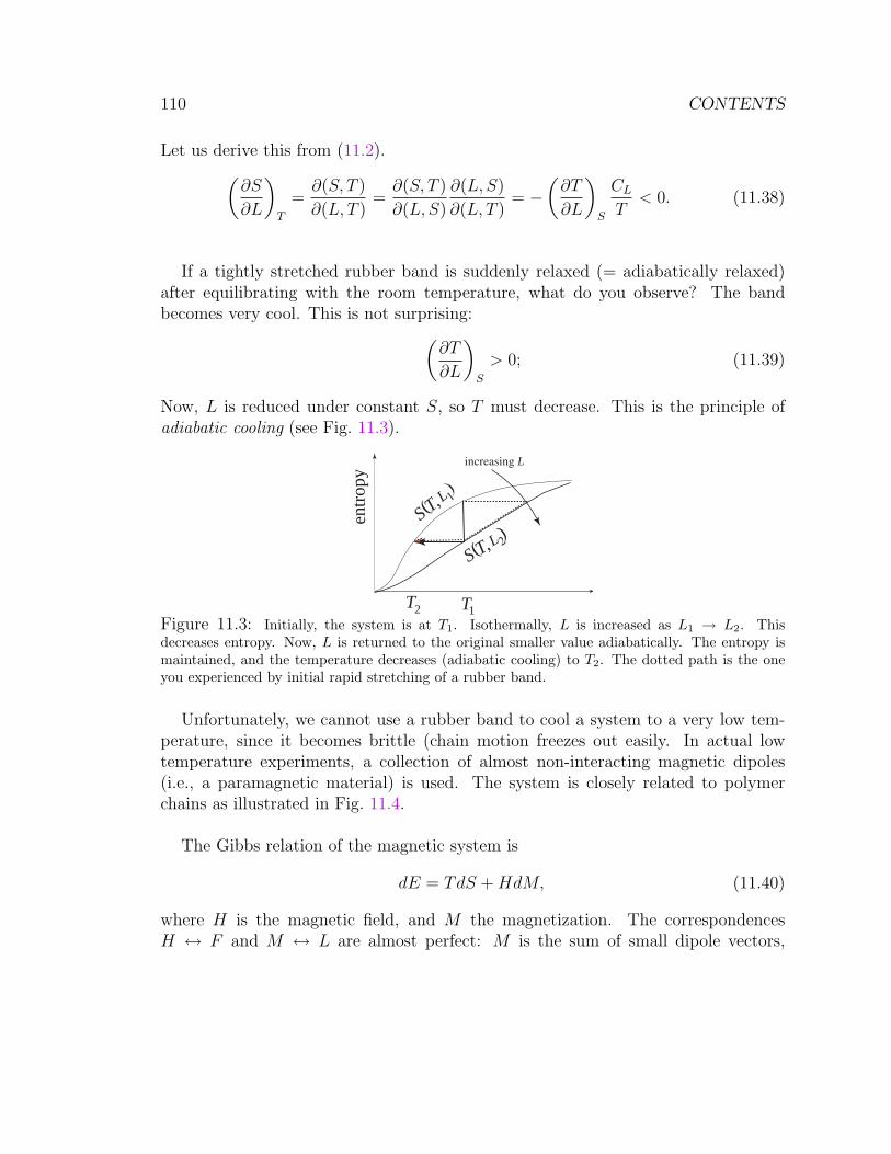
110 CONTENTS
Let us derive this from (11.2).(∂S
∂L
)T
=∂(S, T )
∂(L, T )=∂(S, T )
∂(L, S)
∂(L, S)
∂(L, T )= −
(∂T
∂L
)S
CL
T< 0. (11.38)
If a tightly stretched rubber band is suddenly relaxed (= adiabatically relaxed)after equilibrating with the room temperature, what do you observe? The bandbecomes very cool. This is not surprising:(
∂T
∂L
)S
> 0; (11.39)
Now, L is reduced under constant S, so T must decrease. This is the principle ofadiabatic cooling (see Fig. 11.3).
TT 12
entr
opy
increasing L
S T,()L 1
S T,()L 2
Figure 11.3: Initially, the system is at T1. Isothermally, L is increased as L1 → L2. Thisdecreases entropy. Now, L is returned to the original smaller value adiabatically. The entropy ismaintained, and the temperature decreases (adiabatic cooling) to T2. The dotted path is the oneyou experienced by initial rapid stretching of a rubber band.
Unfortunately, we cannot use a rubber band to cool a system to a very low tem-perature, since it becomes brittle (chain motion freezes out easily. In actual lowtemperature experiments, a collection of almost non-interacting magnetic dipoles(i.e., a paramagnetic material) is used. The system is closely related to polymerchains as illustrated in Fig. 11.4.
The Gibbs relation of the magnetic system is
dE = TdS +HdM, (11.40)
where H is the magnetic field, and M the magnetization. The correspondencesH ↔ F and M ↔ L are almost perfect: M is the sum of small dipole vectors,
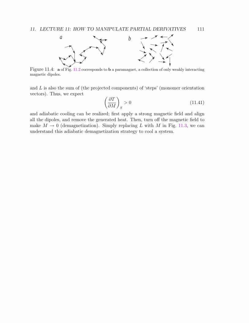
11. LECTURE 11: HOW TO MANIPULATE PARTIAL DERIVATIVES 111
a b
Figure 11.4: a of Fig. 11.2 corresponds to b a paramagnet, a collection of only weakly interactingmagnetic dipoles.
and L is also the sum of (the projected components) of ‘steps’ (monomer orientationvectors). Thus, we expect (
∂T
∂M
)S
> 0 (11.41)
and adiabatic cooling can be realized; first apply a strong magnetic field and alignall the dipoles, and remove the generated heat. Then, turn off the magnetic field tomake M → 0 (demagnetization). Simply replacing L with M in Fig. 11.3, we canunderstand this adiabatic demagnetization strategy to cool a system.
112 CONTENTS
12 Lecture 12: Stability of equilibrium states
Summary∗ We can derive the universal stability (and evolution) criterion δ2S < 0 (> 0) thatis independent of the environmental constraints (say, isothermal, constant volume ornot, etc.)∗ ∂(X, Y )/∂(x, y) > 0.∗ In equilibrium changes occur in the direction to discourage further changes (toavoid run-away processes) (Le Chatelier-Braun principle).∗ Gibbs free energy is a convenient thermodynamic potential to study the systemsunder T , P constant.∗ G =
∑µiNi, and the direction of a chemical reaction can be studied by ∆G due
to reaction.
Key wordsuniversal stability criterion, universal evolution criterion, positive definite quadraticform, Le Chatelier principle, Le Chatelier-Braun principle, Gibbs-Duhem relation.
What you should be able to do∗ To derive the universal stability criterion.∗ To mention some of the crucial conclusions due to the stability criterion (say,CX > 0).∗ To derive the Gibbs-Duhem relation.
Let us perform a few review exercises. What is the sign of(∂S
∂F
)L
(12.1)
for a rubber band? Intuition tells us that it must be positive (To increase F whilekeeping L, we must invigorate the motion of chains, so we must raise the temperature,resulting in the increase of entropy). Let us check this, starting with our empiricalresult (
∂T
∂L
)S
> 0. (12.2)
What you should do first is to rewrite the partial derivative in terms of Jaco-
12. LECTURE 12: STABILITY OF EQUILIBRIUM STATES 113
bians: (∂S
∂F
)L
=∂(S, L)
∂(F,L). (12.3)
(12.2) is (∂T
∂L
)S
=∂(T, S)
∂(L, S), (12.4)
so we should keep (L, S) and insert (T, S):(∂S
∂F
)L
=∂(S, L)
∂(F,L)=∂(S, L)
∂(T, S)
∂(T, S)
∂(F,L)= −∂(S, L)
∂(T, S)=∂(L, S)
∂(T, S)> 0. (12.5)
We have used a Maxwell’s relation.One more for a gas: How about the sign of(
∂S
∂P
)V
? (12.6)
To increase P under constant V , we have to raise the temperature, resulting inthe increase of entropy, so the sign must be positive. The cleverest approach maybe (
∂S
∂P
)V
=∂(S, V )
∂(P, V )=
∂(S, V )
∂(T,−P )
∂(T,−P )
∂(P, V )=
∂(S, V )
∂(T,−P )
/(∂V
∂T
)P
. (12.7)
Therefore, (12.6) and (∂V/∂T )P , which is positive for any gas,83 have the same sign,but to understand this we need the stability result
∂(S, V )
∂(T,−P )> 0. (12.8)
Today’s main dish is the universal stability criterion.Clausius told us that if a spontaneous change occurs in an isolated system,
∆S ≥ 0. (12.9)
83This inequality is not a thermodynamic inequality. That is, it is not due to the principlesof thermodynamics and materials-free general conditions. In contrast, the inequality (12.8) isthermodynamic (universally true). It is important to distinguish these different kinds of inequalitiesin thermodynamics.
114 CONTENTS
We use the standard trick to study a non-isolated system S as a small part of a hugeisolated system (Fig. 12.1) whose intensive variables are kept constant, but their con-jugate extensive variables may be exchanged between S and its surrounding reservoirfreely.
T
P
x
e
e
e
S
Figure 12.1: S is a part of a huge isolated system whose intensive parameters Te, Pe, xe, etc., arekept constant. Their conjugate extensive quantities S (or heat), V , X, etc., can be freely exchangedbetween the system S and the rest.
If something spontaneous can happen, the total entropy must increase. In the sys-tem something irreversible might have happened, so we cannot compute ∆S directlywith the aid of imported quantities ∆E,∆V,∆N , etc. However, for the reservoir,since we assume ti is always in equilibrium, we can write its entropy change as
∆Sres = − 1
Te
∆E − Pe
Te
∆V +xe
Te
∆X +µe
Te
∆N. (12.10)
Here, ∆E, etc., are the quantities seen from the system S (+ for importing), so −∆E,−∆V , etc., are the imported quantities to the reservoir. That is why the signs in(12.10) are different from the usual Gibbs relation. Thus, the total entropy changeis ∆S + ∆Sres:
∆S − 1
Te
∆E − Pe
Te
∆V +xe
Te
∆X +µe
Te
∆N ≥ 0. (12.11)
This is essentially Clausius’ inequality.If the equilibrium state is stable, then
∆S − 1
Te
∆E − Pe
Te
∆V +xe
Te
∆X +µe
Te
∆N < 0. (12.12)
Now, let us look at ∆S in more detail. If the change is very small, we can Taylorexpand ∆S into a power series of δE = ∆E, δV = ∆V , etc. (here ∆ is replaced byδ to make it clear that all changes are small):
∆S = δS + δ2S + · · · . (12.13)
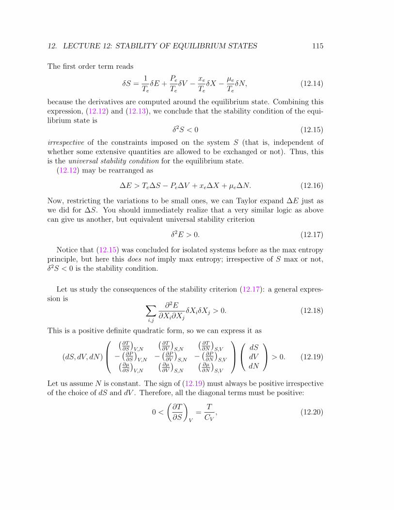
12. LECTURE 12: STABILITY OF EQUILIBRIUM STATES 115
The first order term reads
δS =1
Te
δE +Pe
Te
δV − xe
Te
δX − µe
Te
δN, (12.14)
because the derivatives are computed around the equilibrium state. Combining thisexpression, (12.12) and (12.13), we conclude that the stability condition of the equi-librium state is
δ2S < 0 (12.15)
irrespective of the constraints imposed on the system S (that is, independent ofwhether some extensive quantities are allowed to be exchanged or not). Thus, thisis the universal stability condition for the equilibrium state.
(12.12) may be rearranged as
∆E > Te∆S − Pe∆V + xe∆X + µe∆N. (12.16)
Now, restricting the variations to be small ones, we can Taylor expand ∆E just aswe did for ∆S. You should immediately realize that a very similar logic as abovecan give us another, but equivalent universal stability criterion
δ2E > 0. (12.17)
Notice that (12.15) was concluded for isolated systems before as the max entropyprinciple, but here this does not imply max entropy; irrespective of S max or not,δ2S < 0 is the stability condition.
Let us study the consequences of the stability criterion (12.17): a general expres-sion is ∑
i,j
∂2E
∂Xi∂Xj
δXiδXj > 0. (12.18)
This is a positive definite quadratic form, so we can express it as
(dS, dV, dN)
(
∂T∂S
)V,N
(∂T∂V
)S,N
(∂T∂N
)S,V
−(
∂P∂S
)V,N
−(
∂P∂V
)S,N
−(
∂P∂N
)S,V(
∂µ∂S
)V,N
(∂µ∂V
)S,N
(∂µ∂N
)S,V
dS
dVdN
> 0. (12.19)
Let us assume N is constant. The sign of (12.19) must always be positive irrespectiveof the choice of dS and dV . Therefore, all the diagonal terms must be positive:
0 <
(∂T
∂S
)V
=T
CV
, (12.20)
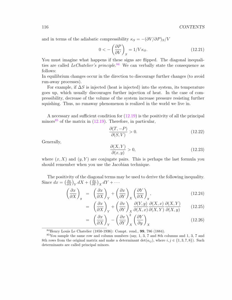
116 CONTENTS
and in terms of the adiabatic compressibility κS = −(∂V/∂P )S/V
0 < −(∂P
∂V
)S
= 1/V κS. (12.21)
You must imagine what happens if these signs are flipped. The diagonal inequali-ties are called LeChatelier’s principle.84 We can verbally state the consequence asfollows:In equilibrium changes occur in the direction to discourage further changes (to avoidrun-away processes).
For example, if ∆S is injected (heat is injected) into the system, its temperaturegoes up, which usually discourages further injection of heat. In the case of com-pressibility, decrease of the volume of the system increase pressure resisting furthersquishing. Thus, no runaway phenomenon is realized in the world we live in.
A necessary and sufficient condition for (12.19) is the positivity of all the principalminors85 of the matrix in (12.19). Therefore, in particular,
∂(T,−P )
∂(S, V )> 0. (12.22)
Generally,∂(X, Y )
∂(x, y)> 0, (12.23)
where (x,X) and (y, Y ) are conjugate pairs. This is perhaps the last formula youshould remember when you use the Jacobian technique.
The positivity of the diagonal terms may be used to derive the following inequality.Since dx =
(∂x∂X
)YdX +
(∂x∂Y
)XdY + · · ·(
∂x
∂X
)y
=
(∂x
∂X
)Y
+
(∂x
∂Y
)X
(∂Y
∂X
)y
, (12.24)
=
(∂x
∂X
)Y
+
(∂x
∂Y
)X
∂(Y, y)
∂(X, x)
∂(X, x)
∂(X, Y )
∂(X, Y )
∂(X, y)(12.25)
=
(∂x
∂X
)Y
−(∂x
∂Y
)2
X
(∂Y
∂y
)X
(12.26)
84Henry Louis Le Chatelier (1850-1936): Compt. rend., 99, 786 (1884).85You sample the same row and column numbers (say, 1, 3, 7 and 8th columns and 1, 3, 7 and
8th rows from the original matrix and make a determinant det(aij), where i, j ∈ 1, 3, 7, 8). Suchdeterminants are called principal minors.
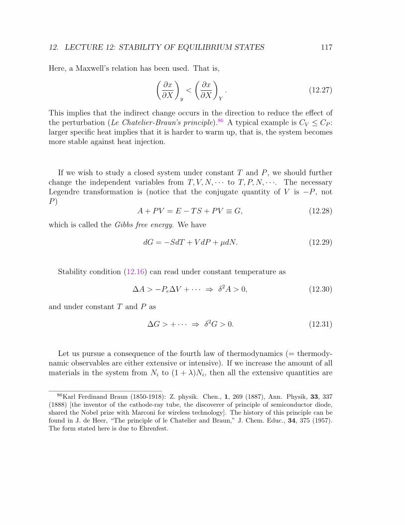
12. LECTURE 12: STABILITY OF EQUILIBRIUM STATES 117
Here, a Maxwell’s relation has been used. That is,(∂x
∂X
)y
<
(∂x
∂X
)Y
. (12.27)
This implies that the indirect change occurs in the direction to reduce the effect ofthe perturbation (Le Chatelier-Braun’s principle).86 A typical example is CV ≤ CP :larger specific heat implies that it is harder to warm up, that is, the system becomesmore stable against heat injection.
If we wish to study a closed system under constant T and P , we should furtherchange the independent variables from T, V,N, · · · to T, P,N, · · ·. The necessaryLegendre transformation is (notice that the conjugate quantity of V is −P , notP )
A+ PV = E − TS + PV ≡ G, (12.28)
which is called the Gibbs free energy. We have
dG = −SdT + V dP + µdN. (12.29)
Stability condition (12.16) can read under constant temperature as
∆A > −Pe∆V + · · · ⇒ δ2A > 0, (12.30)
and under constant T and P as
∆G > + · · · ⇒ δ2G > 0. (12.31)
Let us pursue a consequence of the fourth law of thermodynamics (= thermody-namic observables are either extensive or intensive). If we increase the amount of allmaterials in the system from Ni to (1 + λ)Ni, then all the extensive quantities are
86Karl Ferdinand Braun (1850-1918): Z. physik. Chen., 1, 269 (1887), Ann. Physik, 33, 337(1888) [the inventor of the cathode-ray tube, the discoverer of principle of semiconductor diode,shared the Nobel prize with Marconi for wireless technology]. The history of this principle can befound in J. de Heer, “The principle of le Chatelier and Braun,” J. Chem. Educ., 34, 375 (1957).The form stated here is due to Ehrenfest.
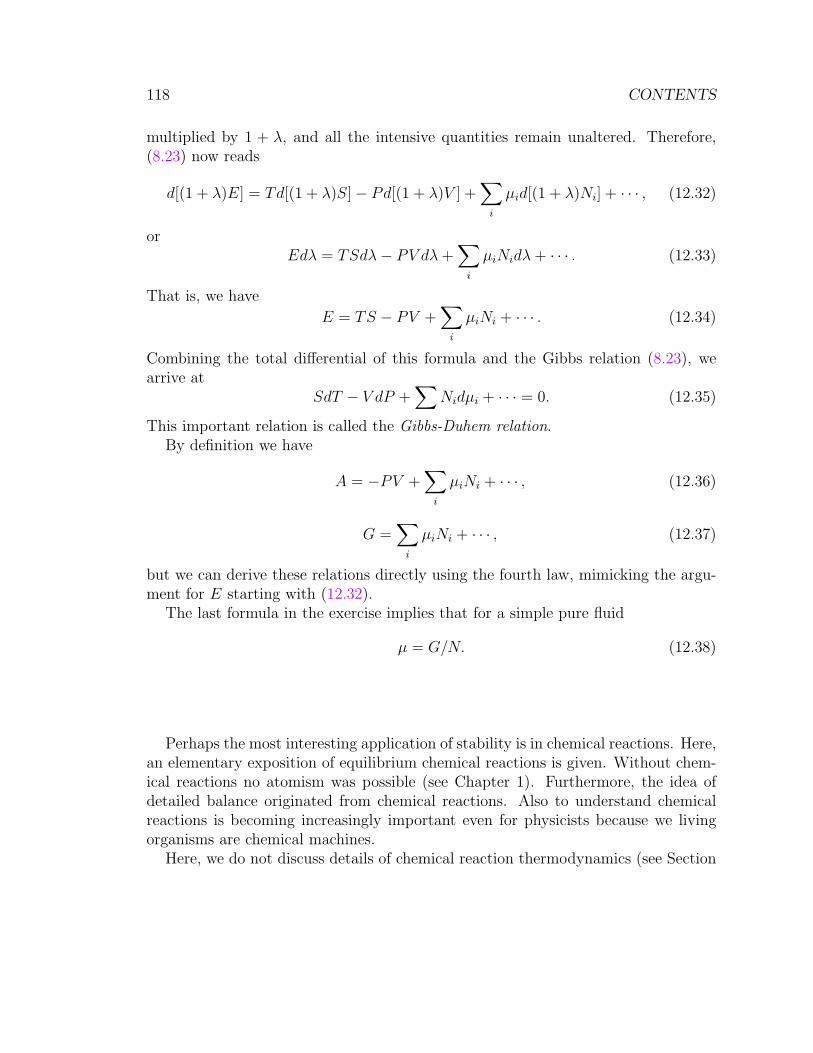
118 CONTENTS
multiplied by 1 + λ, and all the intensive quantities remain unaltered. Therefore,(8.23) now reads
d[(1 + λ)E] = Td[(1 + λ)S]− Pd[(1 + λ)V ] +∑
i
µid[(1 + λ)Ni] + · · · , (12.32)
orEdλ = TSdλ− PV dλ+
∑i
µiNidλ+ · · · . (12.33)
That is, we have
E = TS − PV +∑
i
µiNi + · · · . (12.34)
Combining the total differential of this formula and the Gibbs relation (8.23), wearrive at
SdT − V dP +∑
Nidµi + · · · = 0. (12.35)
This important relation is called the Gibbs-Duhem relation.By definition we have
A = −PV +∑
i
µiNi + · · · , (12.36)
G =∑
i
µiNi + · · · , (12.37)
but we can derive these relations directly using the fourth law, mimicking the argu-ment for E starting with (12.32).
The last formula in the exercise implies that for a simple pure fluid
µ = G/N. (12.38)
Perhaps the most interesting application of stability is in chemical reactions. Here,an elementary exposition of equilibrium chemical reactions is given. Without chem-ical reactions no atomism was possible (see Chapter 1). Furthermore, the idea ofdetailed balance originated from chemical reactions. Also to understand chemicalreactions is becoming increasingly important even for physicists because we livingorganisms are chemical machines.
Here, we do not discuss details of chemical reaction thermodynamics (see Section
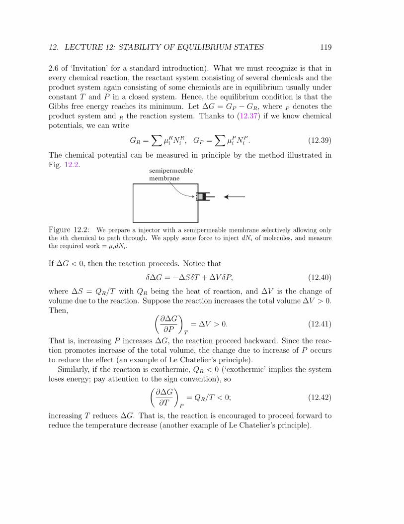
12. LECTURE 12: STABILITY OF EQUILIBRIUM STATES 119
2.6 of ‘Invitation’ for a standard introduction). What we must recognize is that inevery chemical reaction, the reactant system consisting of several chemicals and theproduct system again consisting of some chemicals are in equilibrium usually underconstant T and P in a closed system. Hence, the equilibrium condition is that theGibbs free energy reaches its minimum. Let ∆G = GP − GR, where P denotes theproduct system and R the reaction system. Thanks to (12.37) if we know chemicalpotentials, we can write
GR =∑
µRi N
Ri , GP =
∑µP
i NPi . (12.39)
The chemical potential can be measured in principle by the method illustrated inFig. 12.2.
semipermeable
membrane
Figure 12.2: We prepare a injector with a semipermeable membrane selectively allowing onlythe ith chemical to path through. We apply some force to inject dNi of molecules, and measurethe required work = µidNi.
If ∆G < 0, then the reaction proceeds. Notice that
δ∆G = −∆SδT + ∆V δP, (12.40)
where ∆S = QR/T with QR being the heat of reaction, and ∆V is the change ofvolume due to the reaction. Suppose the reaction increases the total volume ∆V > 0.Then, (
∂∆G
∂P
)T
= ∆V > 0. (12.41)
That is, increasing P increases ∆G, the reaction proceed backward. Since the reac-tion promotes increase of the total volume, the change due to increase of P occursto reduce the effect (an example of Le Chatelier’s principle).
Similarly, if the reaction is exothermic, QR < 0 (‘exothermic’ implies the systemloses energy; pay attention to the sign convention), so(
∂∆G
∂T
)P
= QR/T < 0; (12.42)
increasing T reduces ∆G. That is, the reaction is encouraged to proceed forward toreduce the temperature decrease (another example of Le Chatelier’s principle).
120 CONTENTS
13 Lecture 13: Introduction to statistical mechan-
ics
Summary∗ If we have a translation table between mechanical and thermodynamic quantities,we can calculate thermodynamic quantities with the aid of mechanics.∗ The table must include not only mechanical but thermal quantities. The latter issupplied by Boltzmann’s principle: S = kB logw(E,X).∗ With very natural observations as to thermodynamics and mechanics, we can de-rive this principle from dS = d′Q/T .
Key wordsphase space, microstate (classical and quantum), Boltzmann’s principle
What you should be able to do∗ Tell what thermodynamics can and cannot do.∗ Clearly explain the meaning of the quantities appearing in Boltzmann’s principle.∗ Explain why ergodic idea is totally absurd.
You must clearly recognize that the exposition in this series of lectures is quitenovel.
We have learned rudiments of thermodynamics. As you have realized, thermodynam-ics is very powerful when right input is introduced, but it cannot tell you anythingspecific to a particular system. For example, the equation of state or the functionalform of S = S(E, V ) cannot be supplied by thermodynamics. Even in the case of arubber band (∂T/∂L)S > 0 must be supplied, experimentally.
You must clearly know what thermodynamics can do and what not. Thermody-namics can compute the changes of state functions (state variables) between two equi-librium states irrespective of the actual processes that have happened, IF the equa-tion of state of the system is known. Thermodynamics cannot calculate materials-specific (or system-specific) properties.
Since we believe that the microscopic world underlies the world we experience
13. LECTURE 13: INTRODUCTION TO STATISTICAL MECHANICS 121
daily and since the microscopic world is described by mechanics governing numerousparticles in the systems, we should try to compute thermodynamic quantities interms of mechanics. To describe a macrosystem in terms of particle mechanics, wemust expect that we need numerous variables far more than the dimension of thethermodynamic space. Thus, it is a natural guess that we need some statisticalmeans. Thus, statistical mechanics.
However, as I emphasized repeatedly, the macroscopic world is the world governedby the law of large numbers, so if you know how to get the expectation values, we donot need statistics explicitly. We need only the translation table of thermodynamicquantities in terms of mechanical quantities.
We have learned that the most fundamental description of any equilibrium state isin terms of thermodynamic coordinates (E,X), where E is the internal energy and X(collectively) are the work coordinates. They are extensive and meaningful in termsof mechanics. We know E is the system mechanical energy. X may be the volumeV , magnetization M , etc., and can be described in terms of microscopic mechanicalvariables easily and/or naturally. Thus, we can write down the translation table forthermodynamic coordinates relatively easily.
However, thermodynamics is ‘thermo’dynamics. We must also expand the trans-lation table to include thermal quantities, heat or entropy, at least.
The translation table was completed by Boltzmann in the following form, theBoltzmann principle:87
S = kB logw(E,X), (13.1)
where kB is the Boltzmann constant, and w(E,X) is the ‘number’ of ‘microscopicstates (= microstates) compatible with the macrostate (E,X) (here, I will use thesame symbol to denote the collection of microstates compatible with (E,X) in thefollowing). To understand this statement precisely, we must clarify what ‘microstate’means.88
Classical-mechanically,89 the most detailed description of a system is in terms of aset of the canonical variables. The most popular canonical variables are the positionand momentum vectors. For a N -point-mass system, the 6N -dimensional vector
87Some authors define entropy by this formula. However, S is thermodynamically defined, andwe know how to measure ∆S (entropy change). Therefore, we are NOT allowed to do such anarbitrary and sloppy argument, although ‘retroactively’ this is justified.
88You may understand ‘microstate’ corresponds to ‘elementary event’ in probability.89The Feynman Lectures I is a good classical mechanics introduction. Then, read the first volume
of the Landau-Lifshitz series.
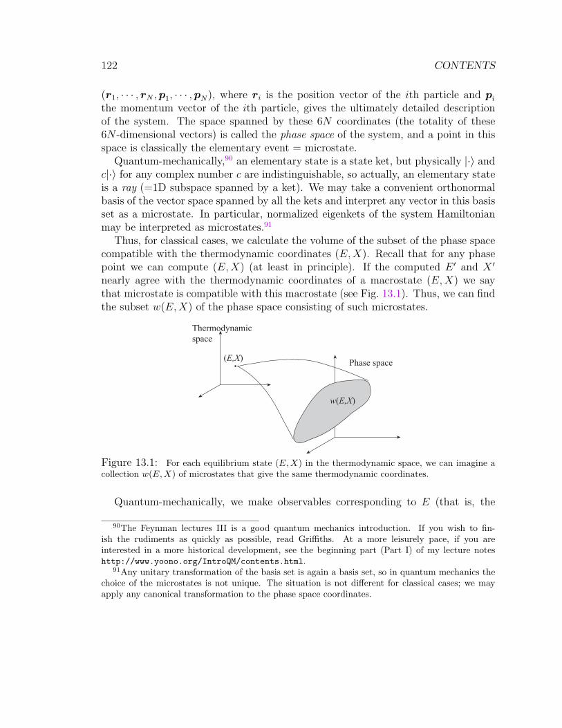
122 CONTENTS
(r1, · · · , rN ,p1, · · · ,pN), where ri is the position vector of the ith particle and pi
the momentum vector of the ith particle, gives the ultimately detailed descriptionof the system. The space spanned by these 6N coordinates (the totality of these6N -dimensional vectors) is called the phase space of the system, and a point in thisspace is classically the elementary event = microstate.
Quantum-mechanically,90 an elementary state is a state ket, but physically |·〉 andc|·〉 for any complex number c are indistinguishable, so actually, an elementary stateis a ray (=1D subspace spanned by a ket). We may take a convenient orthonormalbasis of the vector space spanned by all the kets and interpret any vector in this basisset as a microstate. In particular, normalized eigenkets of the system Hamiltonianmay be interpreted as microstates.91
Thus, for classical cases, we calculate the volume of the subset of the phase spacecompatible with the thermodynamic coordinates (E,X). Recall that for any phasepoint we can compute (E,X) (at least in principle). If the computed E ′ and X ′
nearly agree with the thermodynamic coordinates of a macrostate (E,X) we saythat microstate is compatible with this macrostate (see Fig. 13.1). Thus, we can findthe subset w(E,X) of the phase space consisting of such microstates.
Thermodynamic
space
Phase space
w(E,X)
(E,X)
Figure 13.1: For each equilibrium state (E,X) in the thermodynamic space, we can imagine acollection w(E,X) of microstates that give the same thermodynamic coordinates.
Quantum-mechanically, we make observables corresponding to E (that is, the
90The Feynman lectures III is a good quantum mechanics introduction. If you wish to fin-ish the rudiments as quickly as possible, read Griffiths. At a more leisurely pace, if you areinterested in a more historical development, see the beginning part (Part I) of my lecture noteshttp://www.yoono.org/IntroQM/contents.html.
91Any unitary transformation of the basis set is again a basis set, so in quantum mechanics thechoice of the microstates is not unique. The situation is not different for classical cases; we mayapply any canonical transformation to the phase space coordinates.
13. LECTURE 13: INTRODUCTION TO STATISTICAL MECHANICS 123
system Hamiltonian) and X (we may write X), and then collect eigenkets |·〉 of theHamiltonian whose eigenvalues are close to E and also 〈·|X|·〉 ' X.
We have completely specified the statistical mechanical rule to compute thermo-dynamics. The rest is taken care of by the Gibbs relation
dS =1
TdE +
P
TdV − µ
TdN x
TdX + · · · . (13.2)
In practice, use statistical mechanics sparingly, and use thermodynamics wheneveryou can.
Of course, there are two problems remaining: How to use Boltzmann’s principleand how to understand the principle. Let us use the principle a bit first.
We can use the completed translation table to compute S from mechanics, if youtrust Boltzmann’s principle. Let us study a classical ideal gas. It consists of Nmass points of mass m in a volume V . The system Hamiltonian is the pure kineticenergy:
H =∑
i
p2i
2m. (13.3)
Precisely speaking, w(E, V ) collects all the microstates in the volume V with energyin (E − ∆E,E], where ∆E is a (macroscopically small) leeway (see footnote 94).What we should do first is to formally write down w(E, V ).
w(E, V ) =
∫ri∈V,E−∆E<
Pp2
i /2m≤E
dΓ, (13.4)
where dΓ = dr1 · · · drNdp1 · · · dpN is the volume element of the 6N -dimensionalphase space. The space and momentum integrals can be totally decoupled, so
w(E, V ) =
∫ri∈V,
Pp2
i /2m∈(E−∆E,E]
dΓ (13.5)
=
∫V
dr1 · · ·∫
V
drN
∫P
p2i /2m∈(E−∆E,E]
dp1 · · · dpN (13.6)
= V N
∫P
p2i /2m∈(E−∆E,E]
dp1 · · · dpN . (13.7)
The last integral is the volume of the skin of thickness ∝ ∆E of a 3N−1 dimensional
124 CONTENTS
sphere92 of radius√
2mE, which must be proportional to E3N/2−1∆E, so93
w(E, V ) ∝ V NE3N/2∆E. (13.8)
Here, N 1, so I ignored 1. Therefore, Boltzmann tells us that
S = kB logw = NkB log V +3
2NkB logE + kB log ∆E + · · · , (13.9)
where the remaining terms are N -dependent terms (but we do not change N here).94
Using thermodynamic relations,
1
T=
(∂S
∂E
)V
=3
2
NkB
E(13.10)
or E = (3/2)NkBT . AlsoP
T=
(∂S
∂V
)E
=NkB
V, (13.11)
which is the equation of state. It works!. Boltzmann also used an ideal gas toconclude that his ‘hypothesis’ works as you can see from the small lettered appendixto this lecture.
Incidentally, (13.9) does not satisfy the fourth law: if you double N → 2N , thenE → 2E and V → 2V . Then we must also have S → 2S. When you use statisticalmechanics, a wise practice is to make a shortcut with the aid of thermodynamics.We demand that the fourth law is right. Then, we are forced to accept the followingform:
S = kB logw = NkB logV
N+
3
2NkB log
E
N+ kB log ∆E + · · · . (13.12)
Let us go to a derivation(!) of Boltzmann’s principle starting from empirical factsand some general observation about mechanics. Since we are physicists, and notmetaphysicists, let us be as empirical as possible.(O) If we (thermally) isolate a system, it will eventually arrive at a system that doesnot depend on time (zeroth law).
92Notice that in mathematics, 1-sphere is the edge of a disk, 2-sphere is the skin of a 3D ball (=the ordinary sphere), etc.
93Dimensional analysis can give you this answer as well.94By the way, ∆E can be pretty much anything, if not too small (as ∆E = O[E/eαN ] for some
a > 0).
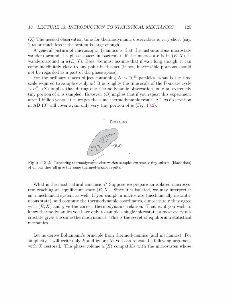
13. LECTURE 13: INTRODUCTION TO STATISTICAL MECHANICS 125
(X) The needed observation time for thermodynamic observables is very short (say,1 µs or much less if the system is large enough).
A general picture of microscopic dynamics is that the instantaneous microstatewanders around the phase space; in particular, if the macrostate is in (E,X), itwanders around in w(E,X). Here, we must assume that if wait long enough, it cancome indefinitely close to any point in this set (if not, inaccessible portions shouldnot be regarded as a part of the phase space).
For the ordinary macro object containing N ∼ 1023 particles, what is the timescale required to sample evenly w? It is roughly the time scale of the Poincare cycle∼ eN . (X) implies that during one thermodynamic observation, only an extremelytiny portion of w is sampled. However, (O) implies that if you repeat this experimentafter 1 billion years later, we get the same thermodynamic result. A 1 µs observationin AD 109 will cover again only very tiny portion of w (Fig. 13.2).
Phase space
w(E,X)
Figure 13.2: Repeating thermodynamic observation samples extremely tiny subsets (black dots)of w, but they all give the same thermodynamic results.
What is the most natural conclusion? Suppose we prepare an isolated macrosys-tem reaching an equilibrium state (E,X). Since it is isolated, we may interpret itas a mechanical system as well. If you sample a microstate (mechanically instanta-neous state), and compute the thermodynamic coordinates, almost surely they agreewith (E,X) and give the correct thermodynamic relation. That is, if you wish toknow thermodynamics you have only to sample a single microstate; almost every mi-crostate gives the same thermodynamics. This is the secret of equilibrium statisticalmechanics.
Let us derive Boltzmann’s principle from thermodynamics (and mechanics). Forsimplicity, I will write only E and ignore X; you can repeat the following argumentwith X restored. The phase volume w(E) compatible with the microstates whose
126 CONTENTS
energy is in (E −∆E,E] may be written as
w =
∫dΓχ∆E(H − E), (13.13)
where χ∆E is the indicator of (−∆E, 0], and dΓ is the phase volume.95 Here, theintegration is over all the phase space of the system. Let us assume that the Hamil-tonian contains a parameter λ that can be controlled externally (to do macroscopicwork, or to regulate work coordinates; λ is something like a handle). The change ofthe Hamiltonian due to the change of the parameter λ → λ + δλ is identified withwork δ′W by Einstein. We can also change E by δE. Thus, notice that
H(λ+ δλ)−H(λ)− δE = δ′W − δE = −δ′Q. (13.14)
Taking account of the internal energy E being also changed by δE as well as λ, weobtain
δw =
∫χ′∆E(H − E)(δ′W − δE) dΓ (13.15)
Since almost all the microstates give the same thermodynamic results as alreadyargued, δ′W − δE is almost always the same for any microstate compatible with agiven thermodynamic state. Therefore, we obtain
δw = (δ′W − δE)
∫χ′∆E(H − E) dΓ, (13.16)
or with the aid of (13.14)
δ logw = −δ′Q∫dΓχ′∆E(H − E)∫dΓχ∆E(H − E)
. (13.17)
Defining
η =
(∂logw
∂E
)X
= −∫dΓχ′∆E(H − E)∫dΓχ∆E(H − E)
, (13.18)
we get (under constant X)d logw = ηd′Q. (13.19)
What is η? Let us compute this quantity for an ideal gas. Actually, we have alreadydone that in (13.10):
kB∂logw(E, V )
∂E=
3kBN
2E. (13.20)
95The quantum version is almost the same with integral replaced by trace.
13. LECTURE 13: INTRODUCTION TO STATISTICAL MECHANICS 127
We know this is 1/T even before thermodynamics was established (recall the Maxwelldistribution). Now we can use thermodynamics δS = δ′Q/T , (and adjusting theunits, if needed), we conclude (13.1)
dS = kBd logw. (13.21)
Integrating this, we obtain Boltzmann’s principle. QED.
If we accept that entropy is a functional of w, then (13.21) is an inescapable con-clusion.
A crucial observation is that entropy is an extensive quantity. If we form a com-pound system by combining two systems I and II already in thermal equilibriumwith each other, the entropy of the compound system is the sum of that of eachcomponent (the fourth law).
The interaction introduced by the contact of the two systems is, for macroscopicsystems, a very weak one. In any case, the effect is confined to the boundary layerwhose thickness is microscopic. Thus, the two subsystems may be regarded statis-tically independent. Therefore, the total number of microstates of the compoundsystem must be very close to the product of the total numbers of microstates for Iand II: w = wIwII.
Combining the above considerations, we have arrived at the following functionalrelation:
S(wIwII) = S(wI) + S(wII), (13.22)
where suffixes denote subsystems.Assuming that S is an increasing function of w, we may conclude from the relation
that S is proportional to logw. Therefore, we have arrived at (13.21). The propor-tionality coefficient kB must be positive, because entropy should be larger with largerE that corresponds to larger w.
We have already discussed the meaning of entropy in terms of the number of yes-no questions to specify the molecular state. From this idea, notice that S ∝ logw isquite natural.
When Boltzmann arrived at his statistical mechanics framework, he thought thatthermodynamic observables are the average value over w. To average, the trajectoryof the system as a mechanical system should sample the subset w evenly, so he con-ceived the so-called ergodicity: the trajectory can visit in any neighborhood of anypoint in w. Almost all the currently popular textbooks explain this totally wrong
128 CONTENTS
idea.As I told you a couple of weeks ago, every ambitious young man attempted to
derive the irreversibility from mechanics. Boltzmann studied the gas dynamic indetailed and ‘demonstrated’ irreversibility. His colleague Loschmidt questioned whytime-reversal symmetric mechanics could gave rise to a system losing this symmetry.Boltzmann realized that there is an approximation to discard memory. Then cameZermelo pointed a logical error: if the phase space (or the portion the mechanicsresides) is virtually bounded (energy is finite, volume is finite), even if memory isdiscarded, still any trajectory can return in any neighborhood of the starting point(Poincare’s recurrence theorem), so irreversibility cannot be concluded. Boltzmanncountered that the young man (= Zermelo) should know physics; can you wait forthat long time of order 10N? Thus, in practice, irreversibility is real, even if thesystem is finite.
However, you must quickly realize that this counterargument backfires. For evensampling of the phase space, you must observe the system for an extremely longtime. That is, ergodicity cannot justify statistical mechanics! Boltzmann must haverealized that he was totally wrong. Indeed, he realized the secret of equilibriumstatistical mechanics: every microstate give the same thermodynamic observables!
Boltzmann’s followers all ignored (or could not understand) this insight.
APPENDIX: How did Boltzmann reach his formula?Let us taste the original paper.96,97 Main steps are stated as questions and answers to them.98 Letus consider a gas consisting of N particles in a container with volume V . Let wn be the numberof particles with the (one-particle) energy between (n − 1)ε and nε (ε > 0). Thus, the set wnspecifies a collection of microstates of the system with wn particles in the one particle energy binwith the energy in ((n− 1)ε, nε].(1) Show that maximizing the number of ways (‘Komplexionszahl’) to realize a collection of mi-crostates (‘Komplexion’) specified by wn is equivalent to the minimization condition for
M =∑
wn log wn. (13.23)
The Komplexionszahl reads
ZK =N !
w1!w2! · · ·wn! · · ·, (13.24)
so maximizing this is equivalent to minimizing the denominator or its logarithm:
log(w1!w2! · · ·wn! · · ·) =∑
n
log wn! =∑
(wn log wn − wn) = M −N. (13.25)
96This is adopted from Equilibrium Statistical Mechanics (ver May 2012).97L. Boltzmann, “Uber die Beziehung zwischen dem zweiten Hauptsatze der mech-
anischen Warmetheorie und der Wahrscheinlichkeitsrechinung respective den Satzen uberWarmegleichgewicht,” Wiener Berichte 76, 373 (1877) (“On the relation between the second lawof thermodynamics and probability calculation concerning theorems of thermal equilibrium”) [Ac-cession of Queen Victoria to ‘Empress of India’ was proclaimed at the Delhi Durbar of 1877.]
98This is almost a copy of my grad course lecture notes.
13. LECTURE 13: INTRODUCTION TO STATISTICAL MECHANICS 129
The original paper kindly discusses that we can discard numerical factors, etc., in Stirling’s formula.(2) Write wi = w(x)ε and simultaneously take the n → ∞ and ε → 0 limits, maintaining x = nεfinite. Show that minimizing M is equivalent to minimizing
M ′ =∫
w(x) log w(x)dx. (13.26)
Substituting the quantities in M as indicated, we have∑n
wn log wn =∑
n
w(x)ε log[w(x)ε] =∑
n
w(x)ε log w(x) +∑
n
w(x)ε log ε (13.27)
The first term is a Riemann sum, so we obtain (13.26). The second term is N log ε and is unrelatedto the number of complexions, so we may ignore it.(3) We should not ignore the constraints that the total number of particles is N and the totalenergy is E. Under this condition, derive Maxwell’s distribution in 3-space by minimizing M ′.
In the original paper Boltzmann regarded the variable x as the three components of velocityvector vx, vy, vz. Here, we take the momentum p and the position r as x: w(x) = w(r,p). Theconstraints are
N =∫
drdp w(r,p), E =∫
drdp w(r,p)E(p), (13.28)
where E(p) = p2/2m is the energy of a single particle state p with m being the mass of a gasparticle. Using Lagrange’s technique, we should maximize (α and β are multipliers)∫
drdp w(r,p)[log w(r,p) + α + βE(p)]. (13.29)
Hence, (E = (3/2)NkBT is used to fix β)
w(r,p) =N
V
1(2πmkBT )3/2
e−p2/2kBTm. (13.30)
Thus, we have obtained the Maxwell distribution.(4) Now, Boltzmann realized that log ZK = log N !−M ′ gives the entropy of the ideal gas. Basedon this finding, he proposed
S ∝ log (Number of ‘Komplexions’). (13.31)
Compare this and the formula for S obtained thermodynamically, as Boltzmann did, to confirm hisproposal.
If we compute (13.31) (i.e., N log N −M ′) with the aid of w
S = N log V + N
(32
+32
log(2πkBTm))
= N log V T 3/2 + const. (13.32)
This agrees with the entropy obtained thermodynamically (apart from log N !; the formula is notextensive). Indeed, the Gibbs relation is
dS =1T
dE +P
TdV, (13.33)
130 CONTENTS
so with the aid of the internal energy E = (3/2)NkBT and the equation of state, we have
S = NkB log T 3/2 + NkB log(V/N) + const. (13.34)
Usually, the story ends here (so did Boltzmann’s original paper). However, being a much deeperthinker than is usually regarded, for a macrosystem described by E and V Boltzmann confirmed thathis formula of entropy (13.1) satisfied the Gibbs relation for general classical many-body systems;in particular, (dE + PdV )/T is a complete differential.
14. LECTURE 14: STATISTICAL MECHANICS OF ISOTHERMAL SYSTEMS131
14 Lecture 14: Statistical mechanics of isothermal
systems
Summary∗ Isothermal systems are handled by the canonical formalism: A = −kBT logZ.∗Microcanonical and canonical formalisms give identical results if the system is large(if logN/N 1).∗ The principle of equal probability allows us to estimate the probabilities of a col-lection of microstates.
Key wordscanonical partition function, microcanonical partition function, Gibbs-Helmholtz for-mula, Stirling’s formula, binomial theorem, multinomial coefficient, Schottky defect,Schottky type specific heat.
What you should be able to do∗ You must be able to compute the microcanonical partition functions and canonicalpartition functions for simple systems.∗ You must remember the Gibbs formula for S (i.e, dS = · · ·).
We have constructed the statistical mechanics for isolated systems = the translationtable between mechanical and thermodynamic quantities: for the thermodynamiccoordinates the correspondence is straightforward. To utilize the Gibbs relation
dE = TdS − PdV + µdN + xdX + · · · , (14.1)
we need the interpretation of S in terms of mechanics. We have derived Boltzmann’sprinciple:
S = kB logw(E,X). (14.2)
w is not very easy to compute, so we will not discuss how to use this very much,but let us do one simple example (another a bit complicated example will be at teend of this lecture to demonstrate the equivalence of canonical and microcanonicalapproaches).
Let us consider an isolated crystal with point defects (vacancies) on the lattice
132 CONTENTS
sites (Schottky defects). To create one such defect we must move an atom from alattice point to the surface of the crystal. The energy cost for this is assumed to beε. Although the number n of vacancies are macroscopic, we may still assume it tobe very small compared to the number N of all lattice sites. Hence, we may assumethat the volume of the system is constant. Therefor for this example, the energyof the system is a macroscopic (thermodynamic) variable which completely specifiesmacrostates.
We must compute w as a function of the total energy E, which is given by
E = nε. (14.3)
We may interpret this as the internal energy. We may consider w as a function of n.A microstate of this system is specified where to put n vacancies. Since all the latticepoints can be distinguished, the number of placing n vacancies is obviously
w(n) =
(N
n
). (14.4)
To compute the entropy with the aid of Boltzmann’s principle, we use Stirling’sformula to evaluate logN ! asymptotically:
N ! ≈(N
e
)N
, (14.5)
orlogN ! ≈ N logN −N. (14.6)
Let us derive (14.6). We start from the gamma function for nonnegative integer N :
Γ(N + 1) =∫ ∞
0
dt tNe−t. (14.7)
To compute this we make the following generating function g(a):
g(a) =∞∑
N=0
aNΓ(N + 1)N !
=∫ ∞
0
dt
∞∑N=0
(at)N
N !e−t =
∫ ∞
0
dt e−(1−a)t =1
1− a=
∞∑N=0
aN . (14.8)
Since a can be anything (although |a| < 1 must be required), we have demonstrated that
Γ(N + 1) = N !. (14.9)
Since N is very large, if we rewrite
Γ(N + 1) =∫ ∞
0
dt tNe−t =∫ ∞
0
dt eN(log t−t/N), (14.10)
14. LECTURE 14: STATISTICAL MECHANICS OF ISOTHERMAL SYSTEMS133
the integrand should be concentrated around the peak of log t − t/N , which is at t = N . There-fore,
N ! =∫ ∞
0
dt eN(log t−t/N) ' eN log N−N . (14.11)
This is what we wanted.
Boltzmann’s principle gives us
S = kB logw ' kB[N logN − n log n− (N − n) log(N − n)]. (14.12)
Incidentally, the following formula is useful (and easy to remember):
log
(A
B
)= −A
[B
Alog
B
A+
(1− B
A
)log
(1− B
A
)]. (14.13)
This gives
S = −NkB
[ nN
logn
N+(1− n
N
)log(1− n
N
)], (14.14)
which is equivalent to (14.12). Using the Gibbs relation, we get (notice that dE =εdn)
1
T=
(∂S
∂E
)V
=1
ε
dS
dn=kB
εlog
N − nn
. (14.15)
If the temperature is sufficiently low or ε is sufficiently large so that ε/kBT 1, theabove formula reduces to
ε
kBT' log
N
n, (14.16)
because N n. Hence, under this low temperature condition, the internal energyE reads
E = εNe−ε/kBT . (14.17)
The constant volume specific heat CV of the system can be obtained as
CV =dE
dT= NkB
(ε
kBT
)2
e−ε/kBT . (14.18)
Notice that CV has a peak at a certain temperature (Fig. 14.1). This type of specificheat is called the Schottky type specific heat, which tells you the energy gap for anelementary excitation in the system. What can you say from the dimensional ana-lytical point of view about the same problem?
134 CONTENTS
2 4 6 8 10
0.1
0.2
0.3
0.4
0.5
T
CV
TPFigure 14.1: The Schottky type specific heat, which has a peak indicating the energy gap of theorder kBTP = ε/2 (the degree of freedom with an excitation energy of this order).
Isolated systems are not so easy to handle, compared with thermostatted systems.We have introduced the Helmholtz free energy A to study thermostatted systems.We have learned that the information as to thermodynamic potential can be com-pletely obtained from A (the equivalence of thermodynamic potentials thanks to theLegendre transformation).
Let us extend the formalism for isolated systems to thermostatted systems. Thelogic we use is the familiar one: we regard the system as a small portion I of abig isolated system, and assume that the system can freely exchange heat with itssurroundings II.
The total energy E0 of the system is given by
E0 = EI + EII. (14.19)
The number of microstates for system I (resp., II) with energy EI (resp., EII) isdenoted by wI(EI) (resp., wII(EII)). Thermal contact is a very weak interaction, sothe two systems are statistically independent. Hence, the number of microstates forthe compound system with the energies EI in I and EII in II is given by
wI(EI)wII(EII). (14.20)
The total number w(E0) of microstates for the compound system must be the sumof this product over all the ways to partition energy between I and II. Therefore, weget
w(E0) =∑
0≤EI≤E0
wI(EI)wII(E0 − EI). (14.21)
The system II is huge compared with I. Expand the entropy as follows:
SII(E0 − E) = SII(E0)− E∂SII∂EII
+1
2E2∂
2SII∂E2
II+ · · · (14.22)
14. LECTURE 14: STATISTICAL MECHANICS OF ISOTHERMAL SYSTEMS135
and denote the temperature of the heat bath (i.e., system II) by T :
∂SII∂EII
=1
T. (14.23)
We wish to use this formula in equilibrium, so E should be close to the internalenergy of system I. Therefore, due to the extensivity of internal energy this shouldbe of order NI, the total number of particles in the system I. Therefore,
E ∂SII∂EII
= O[NI]. (14.24)
The second derivative in (14.22) should be of order N−1II :
E2∂2SII∂E2
II= −E2 1
T 2CV II= O[NI]O[NI/NII] O[NI], (14.25)
where CV II is the heat capacity of II which is of order NII. Therefore, the ratio ofthe second term and the third term in (14.22) is of order NI/NII, which is negligiblysmall. Thus, (14.21) reads
w(E0) ' eSII(E0)/kB∑E
wI(E)e−βE , (14.26)
orw(E0)e
−SII(E0)/kB '∑E
wI(E)e−βE , (14.27)
where a standard notationβ = 1/kBT (14.28)
is used.With the aid of Boltzmann’s principle, we have
kB logw(E0) = SI(EI) + SII(EII), (14.29)
so (from now on let’s drop the suffix I to denote the system)
kB log[w(E0)e−SII(E0)/kB ] = S(E) +SII(E0−E)−SII(E0) = S(E)−E/T = −A(T ),
(14.30)where E is the internal energy of the system.
Thus, we have arrived at the following fundamental relation: Let
Z =∑E
w(E)eβE . (14.31)
136 CONTENTS
Then,A = −kBT logZ. (14.32)
Z is called the canonical partition function.
A more microscopic expression is also possible:
Z =∑
all microstates
e−βE = Tr e−βH. (14.33)
If we decompose the sum as follows, we can easily understand this formula:∑all microstates
=∑E
∑all microstates with energy ∼E
, (14.34)
but ∑all microstates with energy ∼E
e−βE = w(E)e−βE . (14.35)
The conventional more or less standard statistical mechanics assumes a principlecalled the principle of equal probability: if we sample a microstate from w(E,X)every microstate is equally probable. Why this principle may be used to understandthermodynamic quantities is explained in Appendix. If we accept this principle, thenin each w(E,X) the probability to sample any subset u ∈ w(E,X) is proportionalto its phase volume (classically) or number of states in it (quantum case). Thus, wecan interpret that the probability for a microstate γ is
P (γ) =1
Ze−βH(γ). (14.36)
This is called the canonical distribution. As can be seen from its derivation below,you are not allowed to use this to study microscopic properties of the system unlessthey are really statistically independent as in ideal gases.
Once the canonical partition function is known, the internal energy of the systemcan be obtained easily:
E = 〈E〉 =∑E
P (E)E =1
Z
∑E
EwI(E)e−βE = −∂logZ(β)
∂β, (14.37)
where Z (cf. (14.33)) is explicitly written as a function of β.
14. LECTURE 14: STATISTICAL MECHANICS OF ISOTHERMAL SYSTEMS137
The Gibbs relation reads
dS = (1/T )dE + (P/T )dV − (x/T )dX, (14.38)
sod(S − E/T ) = −Ed(1/T ) + (P/T )dV − (x/T )dX, (14.39)
which is a Legendre transformation applied to entropy. This means
− d(A/T ) = −Ed(1/T ) + (P/T )dV − (x/T )dX (14.40)
or− d(βA) = d logZ = −Edβ − (βP )dV + (βx)dX. (14.41)
This tells us that (14.37) is a thermodynamically well-known formula:(∂(A/T )
∂(1/T )
)V
= E, or
(∂βA
∂β
)V
= E, (14.42)
the Gibbs-Helmholtz formula. Do not forget that this is a purely thermodynamicrelation.
Example: Schottky defects revisitedLet’s revisit the Schottky defects. With w(n) known (see (14.4)), it is easy to computeZ:
Z =∑
n
w(n)e−βnε = (1 + e−βε)N , (14.43)
where we have used the binomial theorem:
(x+ y)N =N∑
n=0
(N
n
)xnyN−n. (14.44)
For a demonstration, see 1.2A.4 in ‘Invitation.’ Thus,
N∑n=0
w(n)e−βnε =∑
n
(N
n
)e−βnε1N−n = (1 + e−βε)N . (14.45)
However, you can probably write down the right-most formula directly: the canonicalpartition function is a sum over all the possible microstates
Z =∑
ε(1)∈0,ε,···,ε(N)∈0,ε
e−βPN
i=1 ε(i), (14.46)
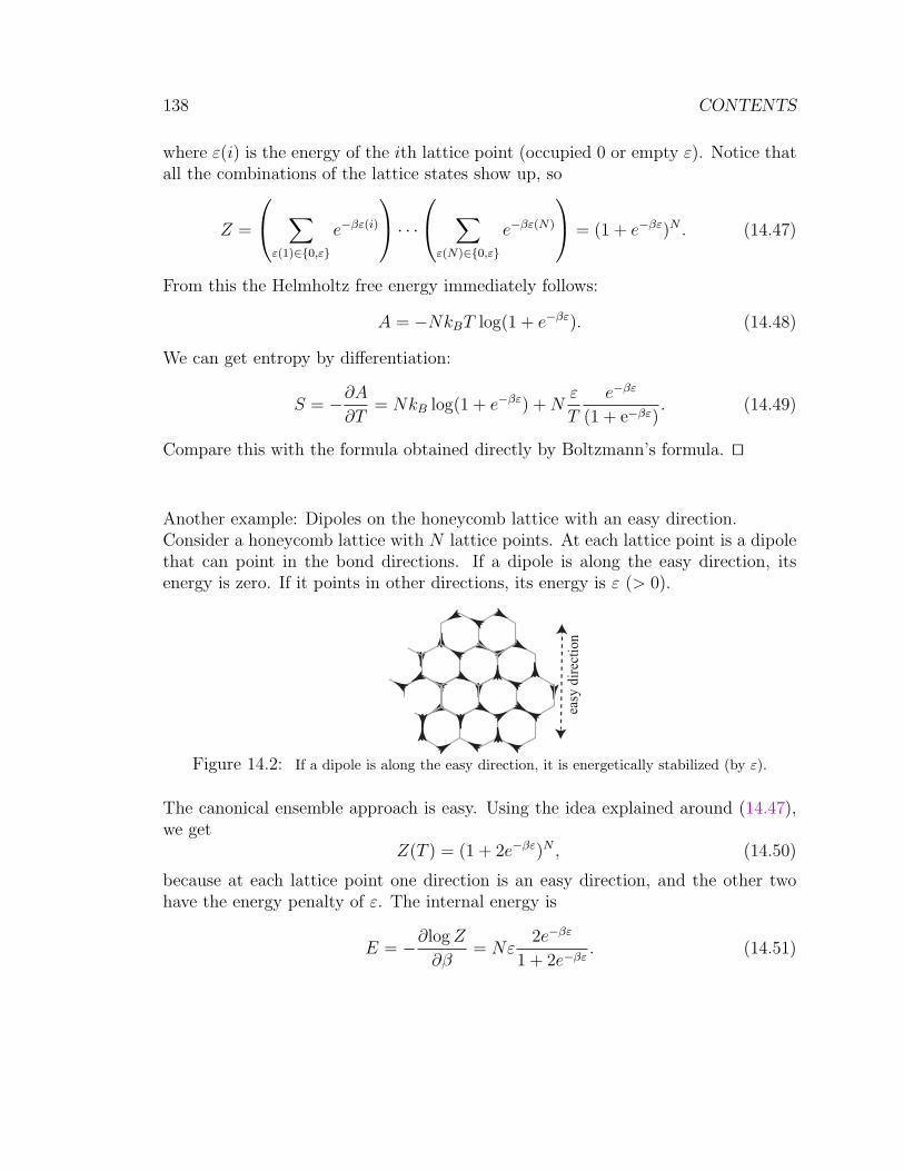
138 CONTENTS
where ε(i) is the energy of the ith lattice point (occupied 0 or empty ε). Notice thatall the combinations of the lattice states show up, so
Z =
∑ε(1)∈0,ε
e−βε(i)
· · · ∑
ε(N)∈0,ε
e−βε(N)
= (1 + e−βε)N . (14.47)
From this the Helmholtz free energy immediately follows:
A = −NkBT log(1 + e−βε). (14.48)
We can get entropy by differentiation:
S = −∂A∂T
= NkB log(1 + e−βε) +Nε
T
e−βε
(1 + e−βε). (14.49)
Compare this with the formula obtained directly by Boltzmann’s formula. ut
Another example: Dipoles on the honeycomb lattice with an easy direction.Consider a honeycomb lattice with N lattice points. At each lattice point is a dipolethat can point in the bond directions. If a dipole is along the easy direction, itsenergy is zero. If it points in other directions, its energy is ε (> 0).
easy
dir
ecti
on
Figure 14.2: If a dipole is along the easy direction, it is energetically stabilized (by ε).
The canonical ensemble approach is easy. Using the idea explained around (14.47),we get
Z(T ) = (1 + 2e−βε)N , (14.50)
because at each lattice point one direction is an easy direction, and the other twohave the energy penalty of ε. The internal energy is
E = −∂logZ
∂β= Nε
2e−βε
1 + 2e−βε. (14.51)
14. LECTURE 14: STATISTICAL MECHANICS OF ISOTHERMAL SYSTEMS139
With the aid of the principle of equal probability, we can ask the probability fora dipole to be in the leftward tilt:
P (left) =e−βε
1 + 2e−βε. (14.52)
Probability to point in the easy direction is
P (easy) =1
1 + 2e−βε. (14.53)
It is rather stupid to study this system with the microcanonical approach, but letus check that we can obtain the same result. Let A be the state of dipole tilting tothe left, B to the right and C in the easy direction. Let nX (X = A,B or C) be thenumber of dipoles in state X. N = nA + nB + nC . The number of microstates withdefinite nA and nB (nC is determined) is (see 1.2A.3 of ‘Invitation’)
N !
nA!nB!nC !. (14.54)
To obtain the microstates with E = ε(N − nC) = ε(nA + nB), we must collect allpossible nA and nB compatible with the energy condition:
w(ε(N − nC)) =∑
nA+nB=N−nC
N !
nA!nB!nC !=
∑nA+nB=N−nC
N !
(N − nC)!nC !
(N − nC)!
nA!nB!.
=
(N
nC
)N−nC∑nA=0
(N − nC)!
nA!nB!=
(N
nC
)2N−nC .
You should have realized that this is easily obtained as follows. First we choosenC sites to place easy-direction dipoles. There are
(NnC
)ways. Then, choose the
remaining dipoles to tilt leftward or rightward. There are 2N−nC ways. Hence, weobtain the above result.
Thus, the entropy is
S = kB logw(ε(N−nC)) = −NkB
[nC
Nlog
nC
N+(1− nC
N
)log(1− nC
N
)]+(N−nC)kB log 2.
(14.55)With the aid of the Gibbs relation (notice that dE = −εdnC)
1
T=∂S
∂E= −1
ε
∂S
∂nC
=kB
εlog
nC
N − nC
+kB
εlog 2. (14.56)
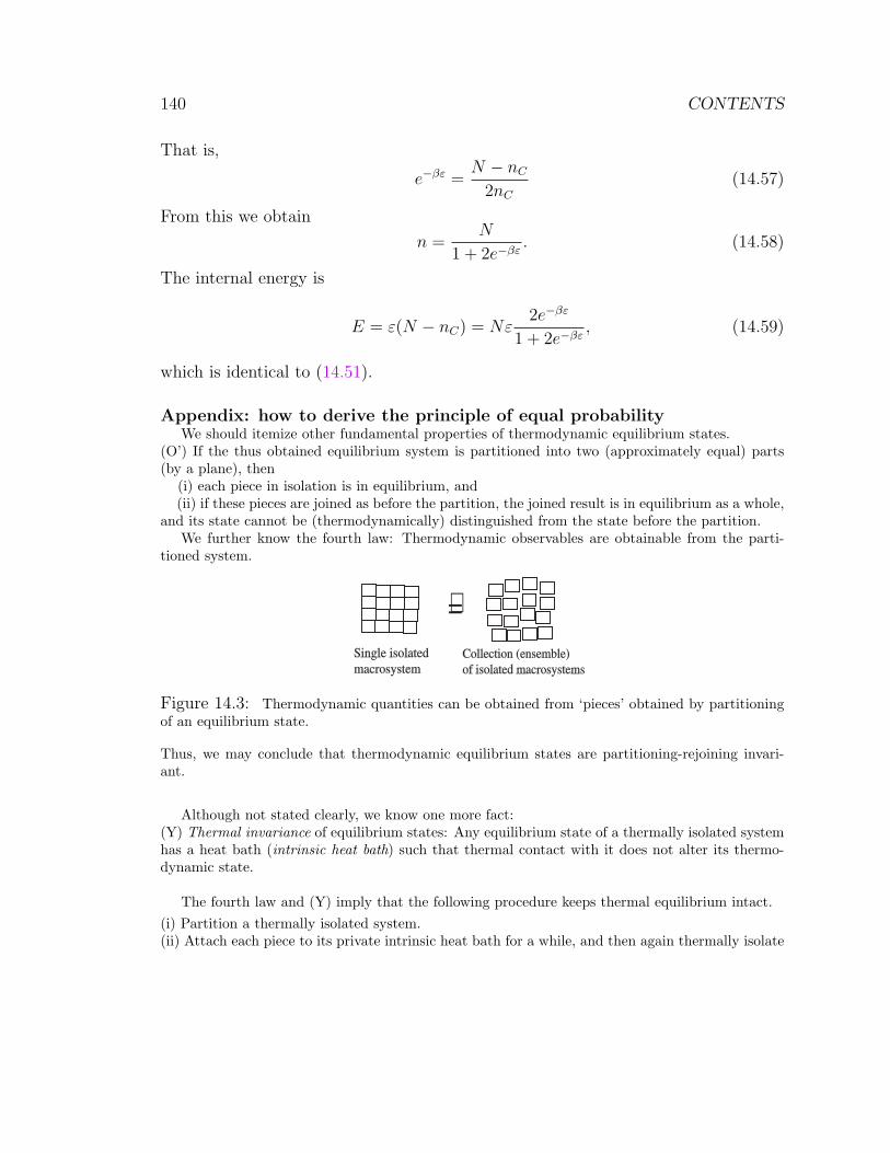
140 CONTENTS
That is,
e−βε =N − nC
2nC
(14.57)
From this we obtain
n =N
1 + 2e−βε. (14.58)
The internal energy is
E = ε(N − nC) = Nε2e−βε
1 + 2e−βε, (14.59)
which is identical to (14.51).
Appendix: how to derive the principle of equal probabilityWe should itemize other fundamental properties of thermodynamic equilibrium states.
(O’) If the thus obtained equilibrium system is partitioned into two (approximately equal) parts(by a plane), then
(i) each piece in isolation is in equilibrium, and(ii) if these pieces are joined as before the partition, the joined result is in equilibrium as a whole,
and its state cannot be (thermodynamically) distinguished from the state before the partition.We further know the fourth law: Thermodynamic observables are obtainable from the parti-
tioned system.
Single isolated
macrosystem
Collection (ensemble)
of isolated macrosystems
=∼
Figure 14.3: Thermodynamic quantities can be obtained from ‘pieces’ obtained by partitioningof an equilibrium state.
Thus, we may conclude that thermodynamic equilibrium states are partitioning-rejoining invari-ant.
Although not stated clearly, we know one more fact:(Y) Thermal invariance of equilibrium states: Any equilibrium state of a thermally isolated systemhas a heat bath (intrinsic heat bath) such that thermal contact with it does not alter its thermo-dynamic state.
The fourth law and (Y) imply that the following procedure keeps thermal equilibrium intact.(i) Partition a thermally isolated system.(ii) Attach each piece to its private intrinsic heat bath for a while, and then again thermally isolate

14. LECTURE 14: STATISTICAL MECHANICS OF ISOTHERMAL SYSTEMS141
Thermally isolated system Intrinsic heat bath
==
Thermodynamically
the same state
Figure 14.4: There is a heat bath that does not destroy a given equilibrium system.
it.(iii) Re-join all the pieces as before to reconstruct the whole piece.
van Hove
partition
Contact with individual
intrinsic heat baths
rejoining
Figure 14.5: An equilibriums system may be replaced by statistically independent pieces toobtain thermodynamic quantities.
The above procedure does not alter thermodynamic observables of the state. Thus, a macro-scopic system in thermal equilibrium may be replaced with a collection of many statistically in-dependent mechanical systems, if we are interested in thermodynamic quantities. In other words,thermodynamics observables are such physical quantities that are quite insensitive to subtle cor-relations (as quantum mechanics implies) among portions of a system. Therefore, we may use abrutal procedure to compute them.
How many such independent pieces can we find in an ordinary macroobject? 1 mm3 is bigenough from the molecules’ point of view, so in a cube with 10 cm edge, we can easily expect morethan106 subsystems; we may safely use the low of large numbers, so thermodynamic quantities donot fluctuate appreciably for such systems.
The reader may even expect that to compute thermodynamic quantities, we may even use theprinciple of equal probability = all the microstates compatible with a given thermodynamic stateare equally probably sampled.
The logic to demonstrate this statement is as follows:(i) The direct product model may be used as a micro-model of a thermodynamic system.(ii) Then, the asymptotic equipartition (see below) implies that the same expectation values areobtained, even if we assume all the energy states are equally probably distributed.(iii) Thus, to obtain thermodynamic, we may assume that all the compatible microstates are equallyprobable. This is called the principle of equal probability traditionally assumed to obtain statisticalmechanics.
The asymptotic equipartition is nothing but the law of large numbers.
1n
log P (x1, · · · , xn) =1n
∑i
log P (xi) converges to s (14.60)

142 CONTENTS
That is, the asymptotic equipartition law:
P (x1, · · · , xn) = ens±o[n]. (14.61)
15. LECTURE 15: CLASSICAL IDEAL GAS AND QUANTUM-CLASSICAL CORRESPONDENCE143
15 Lecture 15: Classical ideal gas and quantum-
classical correspondence
Summary∗ All ensembles are equivalent. You can use any that you can compute most easily.∗ We compute the classical ideal gas partition function. We must treat all gasparticles indistinguishable.∗ The classical canonical partition funciton reads
Z =1
N !h3N
∫dΓ e−βH .
Key wordsensemble, ensemble equivalence, Gibbs paradox, indistinguishability, Frenkel defect
What you should be able to do∗ Get the canonical partition function of a classical gas with dimensional analysis.∗ Be able to explain what the ensemble equivalence means, and the condition thatwe can use any ensemble.
Review:
S = kB logw(E,X) microcanonical formalism, (15.1)
A = −kBT logZ(T,X) canonical formalism. (15.2)
These formalisms are equivalent if logN/N 1. The meaning of ‘equivalence’ is:The free energy computed from S according to (15.1) agrees with that computeddirectly from statistical mechanics according to (15.2); The entropy computed fromA according to (15.2) agrees with S directly computed statistical mechanically from(15.1). In short, you may use any ‘ensemble,’ Here, ‘ensemble’ means the collectionof microscopic states with a definite summation rule (or probability assignment, ifwe use the principle of equal probability).
The principle of equal probability implies that the probability of a microstate γis given by
P (γ) =1
Ze−bH(γ), (15.3)
where H(γ) is the energy of γ.

144 CONTENTS
Let us study an example: the Frenkel defects. As illustrated in Fig. 15.1 particlesleave their original lattice points and wader into non-lattice positions (interstitialpositions). There are N lattice points and M interstitial points. There are totalN particles and n particles leave their lattice points and move into interstitial sites.There is an energy cost of ε to leave a lattice point to move to an interstitial site.The system energy is E = nε. Thus, (we write w(E) as w(n))
Figure 15.1: Particles with darker color are interstitial particles (excited particles), which leavevacancies.
w(n) =
(N
n
)(M
n
), (15.4)
and the canonical partition function reads
Z(T ) =N∑
n=0
w(n)e−βnε =N∑
n=0
(N
n
)(M
n
)e−βnε. (15.5)
Unfortunately, I cannot sum this in a closed form. However, in this case, it isvery easy to prove the ensemble equivalence as follows. Since all the summands arepositive, the following inequalities are obvious:
maxn
[w(n)e−βnε
]≤ Z(T ) ≤ N max
n
[w(n)e−βnε
]. (15.6)
On the other hand, we have
maxn
[w(n)e−βnε
]= exp
[1
kB
maxE
(S − E/T )
], (15.7)
but the ‘honest’ definition of the Helmholtz free energy is
− A = maxE
[TS − E]. (15.8)
15. LECTURE 15: CLASSICAL IDEAL GAS AND QUANTUM-CLASSICAL CORRESPONDENCE145
Therefore, (15.6) reads
− A/kBT ≤ logZ(T ) ≤ −A/kBT + logN. (15.9)
A is an extensive quantity, so it is of order N . Therefore, if you can ignore logN/Nas very small, −kBT logZ(T ) (the free energy directly obtained from statistical me-chanics) and the free energy obtained (using thermodynamics) from entropy (whichis computed statistical-mechanically) are indistinguishable. Although our demon-stration relies on a particular example, the logic we have employed is the key logicto demonstrate the ensemble equivalence generally and rigorously.
You must clearly recognize that the estimations used in statistical mechanics arevery crude. That is why the results are general and very stable.
Let us continue the Frenkel defect problem. Let us compute entropy using Boltz-mann’s principle.
S = kB log
(N
n
)(M
n
). (15.10)
We use Stirling’s approximation, or
log
(A
B
)= −A
[B
AlogBA+
(1− B
A
)log
(1− B
A
)]. (15.11)
We obtain
S/kB = −N[ nN
logn
N+(1− n
N
)log(1− n
N
)]−M
[ nM
logn
M+(1− n
M
)log(1− n
M
)].
(15.12)We need temperature, so we use the Gibbs relation dS = (1/T )dE + (P/T )dV +· · ·:
1
kBT=
(∂S
∂E
)V
, (15.13)
but dE = εdn,99 so
ε
kBT=dS
dn= log
1− nN
nN
+ log1− n
MnM
= log(N − n)(M − n)
n2. (15.14)
Here, notice that when you differentiate log(
Nn
)wrt n, virtually you have only to
differentiate the factors outside log. Usually n is small, we obtain
e−βε =n2
NM. (15.15)
99S is now a function of E, but we do not write it explicitly.
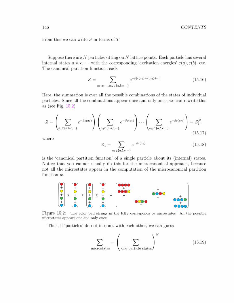
146 CONTENTS
From this we can write S in terms of T
Suppose there are N particles sitting on N lattice points. Each particle has severalinternal states a, b, c, · · · with the corresponding ‘excitation energies’ ε(a), ε(b), etc.The canonical partition function reads
Z =∑
a1,a2,···,aN∈a,b,c,···
e−β[ε(a1)+ε(a2)+···] (15.16)
Here, the summation is over all the possible combinations of the states of individualparticles. Since all the combinations appear once and only once, we can rewrite thisas (see Fig. 15.2)
Z =
∑a1∈a,b,c,···
e−βε(a1)
∑a2∈a,b,c,···
e−βε(a2)
· · · ∑
aN∈a,b,c,···
e−βε(aN )
= ZN1 ,
(15.17)where
Z1 =∑
a1∈a,b,c,···
e−βε(a1) (15.18)
is the ‘canonical partition function’ of a single particle about its (internal) states.Notice that you cannot usually do this for the microcanonical approach, becausenot all the microstates appear in the computation of the microcanonical partitionfunction w.
+
+
+
+
+
+
+
+
+
+
+
+ =x x x
+
+ +
+
+
+
+
+
Figure 15.2: The color ball strings in the RHS corresponds to microstates. All the possiblemicrostates appears one and only once.
Thus, if ‘particles’ do not interact with each other, we can guess
∑microstates
=
∑one particle states
N
(15.19)
15. LECTURE 15: CLASSICAL IDEAL GAS AND QUANTUM-CLASSICAL CORRESPONDENCE147
Let us pursue this strategy for the time being and study the classical ideal gas.
The classical ideal gas is characterized by the total absence of quantum effect:here, quantum effect means that the particles can delocalize. Consider a gas con-sisting of N identical noninteracting particles. Thus, to ignore all quantum effects,the average de Broglie wave length of each particle must be much smaller thanthe average interparticle distance. The de Broglie wave length λ is, on average,(λ = h/p = h/
√2mE and E ∼ kBT )
λ ∼ h/√mkBT , (15.20)
where m is the mass of the particle, and h is Planck’s constant. The mean particledistance is 3
√V/N , so the condition we want is
N
V(mkBT
h2
)3/2
. (15.21)
When this inequality is satisfied, we say the gas is classical.100
Since there are no interactions between particles, each particle cannot sense thedensity. Consequently, the internal energy of the system must be a function of Tonly: E = E(T ). This is a good characterization of ideal gases.
Let us first compute the number of microstates allowed to a single particle in abox of volume V . To this end we solve the Schrodinger equation in a cube with edgesof length L:
− ~2
2m∆ψ = Eψ; (15.22)
∆ is the Laplacian, and a homogeneous Dirichlet boundary condition ψ = 0 at thewall is imposed. As is well-known, the eigenfunctions are:
ψk ∝ sin kxx sin kyy sin kzz, (15.23)
and the boundary condition that the wave function vanishes at the wall requires thefollowing quantization condition:
k ≡ (kx, ky, kz) =π
L(nx, ny, nz) ≡
π
Ln. (15.24)
100Notice that the dynamics of internal degrees of freedom such as vibration and rotation neednot be classical as we will see later.
148 CONTENTS
Here, nx, · · · are positive integers, 1, 2, · · ·. The eigenfunction ψk belongs to theeigenvalue (energy) k2~2/2m.
The number of states with wave vectors k in the range k to k + dk is
#k | k < |k| < k + dk = #
n
∣∣∣∣ Lπ k < |n| < L
π(k + dk)
=
(1
84πn2dn =
)1
8
L3
π34πk2dk =
1
2π2V k2dk. (15.25)
The factor 1/8 is required because the relevant k are only in the first octant (all thecomponents must be positive).
Now we can compute the canonical partition function for a single particle usingits definition:
Z1 =∑
nx>0,ny>0,nz>0
exp(−βE) ' 1
8
V
π3
∫ ∞
0
4πk2dk exp(−βk2~2/2m). (15.26)
The integration is readily performed:
Z1(V ) = V
(2πmkBT
h2
)3/2
. (15.27)
Actually, (15.26) is
Z1(V ) = V1
8π3
∫ ∞
−∞dkx e
−k2x~2/2mkBT
∫ ∞
−∞dky e
−k2y~2/2mkBT
∫ ∞
−∞dkz e
−k2z~2/2mkBT ,
(15.28)and we know ∫ ∞
−∞dx e−ax2
=
√π
a. (15.29)
Therefore,
Z1(V ) = V1
8π3
(2πmkBT
~2
)3/2
= V
(1
4π2
)3/2(8π3mkBT
h2
)3/2
. (15.30)
This is (15.27). The important point of this result is that Z1 ∝ V .
According to our preliminary discussion around (15.19) the partition function Zof the whole ideal gas system consisting of N identical particles should read
“Z = ZN1 ”. (15.31)
15. LECTURE 15: CLASSICAL IDEAL GAS AND QUANTUM-CLASSICAL CORRESPONDENCE149
This impliesA(N, V ) = −NkBT logZ1(V ). (15.32)
Now, prepare two identical systems each of volume V with N particles. The freeenergy of each system is given by A(N, V ). Next, combine these two systems to makea single system. The resultant system has 2N particles and volume 2V , so its freeenergy should be A(2N, 2V ). The fourth law of thermodynamics requires that
A(2N, 2V ) = 2A(N, V ). (15.33)
Unfortunately, as you can easily check, this is not satisfied by (15.32). Z1 ∝ V isthe key feature, so let us write Z1 = cV . Then, Z = (cV )N , so indeed
log(c2V )2N = 2 log(cV )N + log 22N 6= 2 log(cV )N . (15.34)
Thus we must conclude (15.31) is wrong. This is the famous Gibbs paradox.Since the fourth law is an empirical fact, we must modify (15.31) to
Z = f(N)ZN1 = f(N)(cV )N , (15.35)
where f(N) is as yet an unspecified function ofN . The fourth law demands (15.33):
log f(2N) + 2N log(c2V ) = 2 log f(N) + 2N log(cV ). (15.36)
That is,log f(2N) + 2N log 2 = 2 log f(N) (15.37)
orf(N)2 = 22Nf(2N) (more generally, f(N)α = ααNf(αN)). (15.38)
The general solution to this functional equation is (set α = 1/N)
f(N) =
(f(1)
N
)N
∝ (N !)−1. (15.39)
Therefore, thermodynamics forces us to write
Z =1
N !ZN
1 , (15.40)
where we have discarded the unimportant multiplicative factor.
Why do we need 1/N ! for gases and not for lattice systems? The most importantdifference is: while in the case of the lattice system each particle cannot move in
150 CONTENTS
space but simply sits on, say, a lattice point, each gas particle can move around. SeeFig. 15.3. The combinatorial interpretation of N ! (N ! = NPN = P (N,N)) impliesthat the configuration (1) and (2) are distinguishable, but (3) and (4) are not.
We must conclude that each gas particle is indistinguishable from other particles.A configuration of gas particles is just like one pattern on a TV screen; each pixelis indistinguishable. Thermodynamics has forced us to abandon the naive realism;molecules are not the same as the macroscopic objects whose distinguishability wetake for granted.
1 1
0
00 2
0
1 0
1 1
0
0 0
2 1
0
0
12
34
5
6
1
2
3
4
5
6
(1) (2) (3) (4)harmonic oscillators
numbers are quantum numbers
gas particles
numbers denote `different' particles
Figure 15.3: (1) and (2) are distinguishable, but (3) and (4) are not.
Let’s recap. If we ‘honestly count’ the number of quantum states to obtain themicrocanonical partition function (i.e., w(E,X)), we see (→(15.27))
Z1 =1
h3
∫dr
∫pe−p2/2mkBT . (15.41)
Therefore, the canonical partition function in terms of the phase integral reads
Z =1
h3NN !
∫dΓe−β
Pi p
2i /2m, (15.42)
where dΓ = dq1dq2 · · · dqNdp1dp2 · · · dpN is the phase volume element.The prefactors in front of the phase integral are determined while considering a
particular system (the classical ideal gas), so you may think they are rather ad hoc.However, the factor 1/N ! comes form the indistinguishability of the particles, so aslong as particles wander around, this should not be peculiar to ideal gases. Howabout h3N?Z appears in log, so it must be dimensionless (if not, the free energy shifts ac-
cording to the choice of units, for example). Therefore, in front of the integral whose
15. LECTURE 15: CLASSICAL IDEAL GAS AND QUANTUM-CLASSICAL CORRESPONDENCE151
dimension is (action)3N ([pq] = M(L/T )L = M(L/T )2 × T 101), we must have afactor killing this dimension. The most fundamental quantity in physics that hasthe dimension of action is h. Therefore, since we do not expect that the factor isidiosyncratic to the ideal gas, it is natural to expect 1/h3N to appear. Therefore, wedefine the canonical partition function in terms of the phase integral as follows:
Z =1
h3NN !
∫dΓ e−βH. (15.43)
There is a formal demonstration of this relation, but I have never seen any math-ematically respectable proof.
We did a lot of calculation to get Z1 quantum mechanically. However, dimensionalanalysis almost gives you the same result, or, actually, since we may ignore anyconstant factor, we get the correct result by dimensional analysis. Our starting pointis Z1 ∝ V . This is very natural. To make a dimensionless quantity, we need anotherquantity with the dimension of volume, or rather, if we can find a quantity with thedimension of length, we can use it to make Z dimensionless. What length scales dowe have in this problem? The system size (the box size L) is certainly relevant, butwe have already used it V = L3. There is one more length scale, which we havealready discussed: the de Broglie wave length λ ∼
√mkBT/h2. Therefore,
Z1 ∝ V/λ3 = V
(mkBT
h2
)3/2
. (15.44)
Compare this with (15.27). Needless to say, 1/h3 appears naturally.
101Action is energy times time.

152 CONTENTS
16 Lecture 16: Classical ideal gas and harmonic
solid
Summary∗ Canonical partition approach to classical ideal gas. Compute E first, and then useS = (E − A)/T .∗ Classical harmonic solid violate the third law.
Key wordsclassical harmonic oscillator, third law
What you should be able to doGaussian integral, dissecting partition function into one-particle partition functions.
〈〈Ideal gas thermodynamics from the canonical formalism〉〉We have concluded clas-sically the partition function reads
Z(T ) =1
h3NN !
∫dΓ e−βH , (16.1)
where H is the Hamiltonian of the system. Let us finish classical ideal gas.
Z(T ) =1
h3NN !
∫dΓ e−β
Pi p
2i /2m (16.2)
=1
h3NN !
(∫dq
∫dp e−p2/2mkBT
)N
(16.3)
The single-particle canonical partition function in the parentheses is
Z1 =
∫dq
∫dp e−p2/2mkBT = V (2πmkBT )3/2. (16.4)
Therefore, using Stirling’s approximation N ! = (N/e)N , we have (use∫e−ax2
dx =√π/a)
Z =1
N !ZN
1 =
[eV
N
(2πmkBT
h2
)3/2]N
. (16.5)
16. LECTURE 16: CLASSICAL IDEAL GAS AND HARMONIC SOLID 153
The Helmholtz free energy is given by
A = −NkBT logeV
N− 3
2NkBT log
(2πmkBT
h2
). (16.6)
The Gibbs relation reads
dA = −SdT − PdV + µdN. (16.7)
Therefore,
P = −(∂A
∂V
)T
= kBT/V. (16.8)
You can get S by differentiation, but an easier way is to get E first (logZ =−3
2N log β + · · ·)
E = −∂logZ
∂β=
3
2NkBT (16.9)
and
S = (E − A)/T =3
2NkB +NkB log
eV
N
(2πmkBT
h2
)3/2
. (16.10)
If a particle has internal degrees of freedom, we must multiply the corresponding“internal” partition function Zi to get the one particle partition function Z1
Z1(V ) = Zt(V )Zi. (16.11)
For later convenience V is explicitly specified. This formula can easily be understood,because the energy of a particle is a sum of the kinetic energy of its translationalmotion and the energy of its internal degrees of freedom, E = Et + Ei. Each termin this sum does not share any common variable. Zi does not depend on V , becauseinternal degrees of freedom are not affected by the external environment (if the sys-tem is dilute enough).
〈〈Collection of harmonic oscillators〉〉 Let us imagine 1D harmonic oscillators attachedat every lattice point of a solid consisting of N lattice points. Let us assume that
154 CONTENTS
the oscillating mass is m and the spring constant is k (ω2 = k/m is its angularfrequency). The Hamiltonian reads
H =∑
i
(p2
i
2m+k
2q2i
)=∑
i
1
2m(p2
i +mω2q2i ). (16.12)
The canonical partition function is (there is no 1/N !, because oscillators are fixed attheir own individual sites)
Z = ZN1 , (16.13)
where the one particle partition function Z1 is given by
Z1 =1
h
∫dpdq e−β(p2+mω2q2)/2m =
1
h
(2πm
β
2π
mω2β
)1/2
=kBT
~ω. (16.14)
Therefore,
Z =
(kBT
~ω
)N
. (16.15)
The internal energy is
E = N∂
∂βlog(β~ω) = N/β = NkBT. (16.16)
Therefore,
S = (E − A)/T = NkB +NkB log(kBT/~ω) = NkB log T + const. (16.17)
This implies that S −∞ in the T → 0 limit. This is intuitively unthinkable; com-pared to the state at very low temperature T0, S(T ) − S(T0) = NkB log T/T0 1.To describe the state of a harmonic oscillator do we really need indefinitely largeamount of questions to ask?
This is a good occasion to discuss another principle of thermodynamics: the thirdlaw.
Nernst empirically found that all the entropy changes asymptotically vanish inthe T → 0 limit. In particular, all the derivatives of entropy S vanish as T → 0(Nernst’s law). For example,(
∂S
∂P
)T
=∂(S, T )
∂(P, T )=∂(V, P )
∂(P, T )
∂(S, T )
∂(V, P )=∂(V, P )
∂(P, T )= −
(∂V
∂T
)P
→ 0. (16.18)
16. LECTURE 16: CLASSICAL IDEAL GAS AND HARMONIC SOLID 155
All the specific heat vanishes as T → 0. Nernst concluded that entropy becomesconstant (independent of any thermodynamic variables) in the T → 0 limit. Later,Planck chose this constant to be zero (the concept of absolute entropy).
We adopt the following as the third law of thermodynamics:Reversible change of entropy ∆S vanishes in the T → 0 limit.
156 CONTENTS
17 Lecture 17: Specific heat of solid
Summary∗ Quantization forbids incremental increase of energy, so quantization generally re-duces specific heat.∗ If you take into account the proper dispersion relation of a crystal, quantized har-monic oscillators can explain solid specific heat.
Key wordsquantum harmonic oscillator, Debye model, T 3-law, equipartition of energy, Gibbs(-Shannon) formula for entropy, surprisal
What you should be able to do∗ Explain why quantization usually reduces specific heats.
Consider a crystal made of N atoms, having 3N mechanical degrees of freedom.Small displacements of atoms around their mechanical equilibrium positions shouldbe a kind of harmonic oscillation. Thus, we may regard the crystal as a set of 3Nindependent harmonic oscillators (modes) of various frequencies (due to couplingamong atoms). The canonical partition function of the total system is the productof the canonical partition function for each harmonic mode.
Treating the system completely classically and using the definition of the classicalpartition function (15.43), we get for a single harmonic oscillator
Z1 =1
h
∫dp
∫dqe−β(p2+mω2q2)/2m =
kBT
~ω. (17.1)
The contribution of this oscillator to the internal energy is readily obtained as
E1 = kBT. (17.2)
This is independent of the frequency of the oscillator (see equipartition of energybelow), so the total internal energy of the crystal is simply
E = 3NkBT. (17.3)
17. LECTURE 17: SPECIFIC HEAT OF SOLID 157
If the volume is kept constant, the frequencies are also kept constant. Therefore, theconstant volume specific heat CV is given by
CV = 3NkB, (17.4)
which is independent of temperature, a contradiction to the third law of thermody-namics: ∆S → 0 in the T → 0 limit.
Actual experimental results can be summarized as
CV ∼ T 3 (17.5)
at low temperatures. At higher temperatures (17.4) is correct and is called Dulong-Petit’s law.
We must guess that CV 0 should be a quantum effect. Quantization of energyimplies that you cannot pay the energy cost installments. Since T indicates yourenergy payment capability, if T is smaller, then quantize systems are generally harderto excite. Recall Schottky type specific heat: it goes to zero in the T → 0 limitbecause of the energy gap: to excite the system, you must pay this amount atonce.102
Consider a collection of 3N 1-dimensional harmonic oscillators which are not in-teracting with each other at all.
Let us first examine a single oscillator of frequency ν (angular frequency ω = 2πν).Elementary quantum mechanics tells us that the energy of the system is quantizedas
ε =
(1
2+ n
)~ω, n = 0, 1, 2, · · · . (17.6)
Each eigenstate is nondegenerate. Thus, if we specify the quantum number n, themicrostate of a single oscillator is completely specified. The canonical partitionfunction for a single oscillator reads
Z1 =∞∑
n=0
exp
[−β(
1
2+ n
)~ω]. (17.7)
Using (1− x)−1 = 1 + x+ x2 + x3 + · · · (|x| < 1), we get
Z1 = e−β~ω/2(1− e−β~ω)−1 =
(2 sinh
β~ω2
)−1
. (17.8)
102At higher temperatures, the specific heat again goes to zero in this case, because there isnothing remaining to be excite; even if you are rich, now you have nothing to buy.
158 CONTENTS
There are 3N independent oscillators, so the canonical partition function for thesystem should be
Z = Z3N1 . (17.9)
From (17.9) we obtain
A(N) = 3NkBT log
(sinh
β~ω2
), (17.10)
and103
E =3
2N~ω coth
(β~ω
2
)= 3N
(1
2~ω +
~ωeβ~ω − 1
). (17.11)
Hence, the specific heat is
CV = 3NkB
(~ωkBT
)2eβ~ω
(eβ~ω − 1)2. (17.12)
At sufficiently high temperatures (~ω/kBT 1) quantum effects should not beimportant. As expected we recover the classical result (17.4):
CV → 3NkB. (17.13)
For sufficiently low temperatures (~ω/kBT 1) (17.12) reduces to
CV ' 3NkB
(~ωkBT
)2
e−β~ω. (17.14)
Thus, CV vanishes at T = 0, and the third law behavior is exhibited.
However, CV goes to zero exponentially fast at variance with the empirical law(17.5). It is a rule that whenever there is a finite energy gap ε between the ground andthe first excited states, the specific heat behaves like exp(−βε) at low temperatures.The empirical result (17.5) implies that there is no finite energy gap in a real crystal.
There is a distribution in frequencies as can be seen from Fig. 17.1Not all the oscillations contribute significantly to the low temperature heat capacityof solids. Elastic oscillations in a crystal can be classified into two branches, opticaland acoustic (Fig. 17.2).
103
cothx
2=
ex/2 + e−x/2
ex/2 − e−x/2=
ex/2 − e−x/2 + 2e−x/2
ex/2 − e−x/2= 1 +
2ex − 1

17. LECTURE 17: SPECIFIC HEAT OF SOLID 159
Figure 17.1: Above: The lowest frequency mode; Below: The highest frequency mode.
ω
k
optical branch
acoustic branch
optical mode
acoustic mode
Figure 17.2: The optical modes do not displace the crystal lattice points, but the acoustic modes(here a transversal mode is depicted) displaces unit cells. Thus, we must count the number of unitcells to count the number of degrees of freedom relevant to the low temperature heat capacity.
Only the acoustic modes are relevant. We must study the number of modes with agiven angular frequency about ω.
As can be seen from Fig. 17.1 in a 1D direction the possible wavelengths areλ = 2L, 2L/2, · · · , 2L/N or in wave numbers k = π/L, 2π/L, · · · , Nπ/L. We havealready seen such a sequence before: the de Broglie wave length of a free particleconfined in a box which we used to study the classical ideal gas. This implies we cancompute the number of modes in the volume V just as the number of eigenvalues asfollows: ∫ ω
0
D(ω)dω =1
h3
∫dr
∫|p|≤p(ω)
dp, (17.15)
where p(ω) = ~k = ~ω/c (dispersion relation), and c is the sound speed. Therefore,the number of modes between ω and ω + dω is
D(ω) =V
h34πp(ω)2dp(ω)
dω= 4πV
~3
h3c3ω2 =
1
2π2Vω2
c3(17.16)
Actually, there are one longitudinal and two transversal modes for each ω, the actualnumber is this times 3. In contrast to the classical gas case there are two importantdifference. D(ω) ∝ ω2 holds only for low frequency modes where the material maybe regarded as an elastic body. Furthermore, the wavelength cannot be indefinitelysmall as seen from Fig. 17.1. Debye introduced the following approximation:
D(ω) = Aω2Θ(ωD − ω), (17.17)
160 CONTENTS
where ωD is the Debye cutoff frequency (which is a materials ‘constant’ in goodapproximation) and A is fixed to have the total number of modes (= the totalnumber of degrees of freedom 3N) correctly∫ ωD
0
D(ω)dω = 3N. (17.18)
Therefore, A = 9N/ω3D.
Since we know the energy of the mode with ω (17.11), the total energy is
E =
∫dωD(ω)
(1
2~ω +
~ωeβ~ω − 1
), (17.19)
and from (17.12)
CV = kB
∫dωD(ω)
(~ωkBT
)2eβ~ω
(eβ~ω − 1)2. (17.20)
This behaves just as T 3 in the low temperature limit.
〈〈Equipartition of energy〉〉 We know⟨1
2mv2
x
⟩=
1
2kBT (17.21)
independent of mass. This is an example of equipartition of energy. The most generalform is ⟨
xi∂H
∂xj
⟩= kBTδij, (17.22)
where xi are momentum or position coordinates.104⟨xi∂H
∂xj
⟩=
1
Z
∫dΓxi
[−kBT
∂
∂xj
e−βH
], (17.23)
= − 1
ZkBTxie
−βH
∣∣∣∣|x|→∞
+1
ZkBT
∫dΓ
∂xi
∂xj
e−βH . (17.24)
From this we obtain the law of equipartition of energy for classical kinetic energysuch as (no summation convention implied)⟨
p2i
2m
⟩=
1
2kBT, (17.25)
104More precisely, any canonical variables, so angular momenta are admissible.
17. LECTURE 17: SPECIFIC HEAT OF SOLID 161
or ⟨L2
i
2Ii
⟩=
1
2kBT, (17.26)
where m is the mass, Ii is the i-th principal moment of inertia (i-th eigenvalue ofthe inertial moment tensor) and Li is the corresponding component of the angularmomentum.
If the system is governed by a harmonic potential with a spring constant k, weobtain ⟨
kx2
2
⟩=
1
2kBT. (17.27)
Cyclobutanone rings pucker and the oscillation is described by a quartic potentialU = (α/4)x4. The equipartition law is used as follows:⟨
xdU
dx
⟩= α〈x4〉 = kBT, (17.28)
so 〈U〉 = kBT/4.
〈〈Entropy and information〉〉 Let us finalize our understanding of entropy and ‘infor-mation.’
Using the canonical distribution, let us compute entropy explicitly:
S/kB = β(E − A) (17.29)
= logZ + β1
Z
∑He−βH (17.30)
= logZ − 1
Z
∑e−βH log e−βH (17.31)
= −∑ e−βH
Zlog
e−βH
Z. (17.32)
That is,
S = −kB
∑p log p, (17.33)
where p = e−βH/Z is the canonical density operator, or, similarly, classically
S = −kB
∫dΓ p log p, (17.34)
162 CONTENTS
where p is the canonical distribution function. This is the formula first given byGibbs in his famous book on the foundation of statistical mechanics.
The same formula was proposed by Shannon to quantify information, so (18.4) isoften called Shannon’s formula. It is a convenient occasion to see why such a formulais a good measure of information.105
Let us study how much we can quantify our surprise. − log p is sometimes calledsurprisal, i.e., the extent of surprise we feel when an event with probability p actuallyhappens. If an event with large surprisal actually occurs, since this is very rare, wewould feel a large amount of surprise.
Surprisal may be ‘derived’ as follows. Let f(p) be the extent of surprise we feelwhen we know that the event with probability p actually happens. It should havethe following properties:(i) f(p) > 0.(ii) f(p) is a monotone decreasing function of p.(iii) When independent events happen, the extent of surprise is the sum of that ofeach event: f(p1p2) = f(p1) + f(p2).
These imply f(p) ∝ − log p. Therefore, if we have a set of elementary events ithat have probabilities p1, p2, · · · , pn. Then, the expectation value of the surprisal(the expected amount of surprise we feel) from knowing the actual occurrence of anevent is
I(pi) = −∑
i
pi log pi. (17.35)
This agrees with the formula for entropy obtained by Gibbs.
I recommended you to remember
log
(M
N
)= −M
[N
Mlog
N
M+
(1− N
M
)log
(1− N
M
)]. (17.36)
If we define p = N/M this is just I(p, 1 − p) times M . This I is the informationincrease per particle when you place N particles on M sites. If you wish to knowwhether a site is occupied or not, on the average you must ask I YES-NO questions.
105〈〈Textbook of information theory〉〉 The best textbook of information theory (in English)is T. M. Cover and J. A. Thomas, Elements of Information Theory (Wiley, 1991).
18. LECTURE 18: INFORMATION AND ENTROPY; GRAND CANONICAL ENSEMBLE163
18 Lecture 18: Information and entropy; Grand
canonical ensemble
Summary∗ The Gibbs-Shannon formula for entropy/information is explained.∗ For any Legendre-transformed thermodynamic potential G, we can write a parti-tion function Y such that G = −kBT log Y . The ensemble equivalence holds.∗ In particular, the grand partition function Ξ gives PV/T = kB log Ξ.
Key words(Gibbs-)Shannon formula, grand partition function, bosons and fermions, Bose-Einstein distribution
What you should be able to do∗ Explain why the Shannon formula is plausible.∗ You should be able to construct a convenient partition function to obtain a conve-nient thermodynamic potential.∗ For noninteracting particle systems you should be able to compute the grand par-tition functions.∗ Expectation value of the occupation number of a single particle state for bosonsmust be derived.
We have learnedS = −kB
∑p log p = −kB〈log p〉 (18.1)
where p = e−βH/Z is the canonical distribution function. Here, the summation isover all the microstates. Quantum mechanically, this may be written as
S = −kBTrρ log ρ, (18.2)
where
ρ =1
Ze−βH (18.3)
is called the density operator. Classically
S = −kB
∫dΓ p log p, (18.4)
164 CONTENTS
where p is the canonical distribution function. This is the formula first given by Gibbsin his famous book on the foundation of statistical mechanics. Shannon arrived atthe same formula later when he created information theory, so the formula is calledthe Gibbs-Shannon or Shannon formula.
One interpretation of this formula has already been discussed in terms of ‘sur-prisal.’ If we have a set of elementary events i that have probabilities p1, p2, · · · , pn.Then, the expectation value of the surprisal (the expected amount of surprise wefeel) from knowing the actual occurrence of an event is
−∑
i
pi log pi = −〈log p〉. (18.5)
Another approach is as follows. Let η(m) be the ‘information’ per letter we cansend with a message (letter sequence) that is composed of m distinct letters. Here,the word ‘information’ should be understood intuitively. Let us assume that all theletters are used evenly. Also we assume there is no correlation among the symbols.Then, η(m) must be an increasing function of m; if there are only two letters, wecan send, per letter, the information telling whether 1, 2, 3 or 4, 5, 6 as to theoutcome of a single casting of a dice, but if there are three, then more detailed in-formation: 1, 2, 3, 4 or 5, 6 may be sent by a single letter.
Now, let us use simultaneously the second set consisting of n letters. We couldmake compound symbols by juxtaposing them as ab (just as in many Chinese charac-ters). The information carried by each compound symbol should be η(mn), becausethere are mn symbols. We could send the same message by sending all the left halfsymbols first and then the right half symbols later. The amount of information sentby these methods must be equal, so we must conclude that106
η(mn) = η(m) + η(n). (18.6)
Since η is an increasing function, we conclude
η(n) = c log n, (18.7)
where c > 0 is a constant. Its choice is equivalent to the choice of unit of informationper letter and corresponds to the choice of the base of the logarithm in the formula.
106We must send a message explaining how to combine the transferred signals as a part of themessage, but the length of the needed message is finite and independent of the length of the actualmessage we wish to send, so in the long message limit we may ignore this overhead.
18. LECTURE 18: INFORMATION AND ENTROPY; GRAND CANONICAL ENSEMBLE165
If c = 1, we measure information in nat; if we choose c = 1/ log 2 (i.e., η(n) =log2 n), in bit. 1 bit is an amount of information one can obtain from an answer toa single yes-no question.
We have so far assumed that all the symbols are used evenly, but such uniformityis not usual. What is the most sensible generalization of (18.7)? We can write η(n) =− log2(1/n) bits; 1/n is the probability for a particular letter. − log2(1/n) may beinterpreted as the expectation value of − log2(probability of a letter). This suggestsfor the case with not-equal-probability occurrence of n letters with probabilitiesp1, · · · , pn
η(pi) = −n∑
i=1
pi log2 pi. (18.8)
In this way, Shannon arrive at this formula. Naturalness of this interpretation maybe understood as follows.
Suppose we have m + n symbols: a1, · · · , am and b1, · · · bn. If all show up evenly insentences, the information we gain per letter must be log(m + n), since there aren+m letters. Now, assume that unfortunately you cannot see the suffixes. Then, a1
is the same as a3, etc. What information can you obtain? If a∗ show up, you mustask a single m-choice question. This happens with probability m/(m+n). Therefore,the information you can gain must be
η = η(m+ n)− n
n+mη(n)− m
n+mη(m) = − n
n+mlog
n
n+m− m
n+mlog
m
n+m.
(18.9)This is consistent with (18.8).
We may safely conclude that the amount of (the average) information required topinpoint an elementary event in the sample set Ω is proportional to
η = −∑ω∈Ω
p(ω) log p(ω). (18.10)
If you use log2 (i.e., (1/ log 2) log), this is the information in bits (# of averageYES-NO questions you must ask). If you use kB log, you measure information inenergy unit. The entropy S in bits is, according to Boltzmann’s principle, givenby log2w(E,X). This is the number of yes-no questions you must single out amicrostate. Increasing entropy (∆S > 0) implies that to pinpoint a microstate, youmust ask extra questions corresponding to ∆S.
166 CONTENTS
You might wonder what 0.5 yes-no questions imply How can we ask such a ques-tion? Suppose there are 1 red ball and 999 white balls. How many questions doyou need to determine the colors of all the balls? The total entropy is in this case11.4 bits. That is, you need 0.01 Yes-No questions to determine the color of a singleparticle. Let us assume that initially you only know that there are read and whiteballs only First, we divide the balls into two 500 ball sets and ask if one set youchoose is with all the same color or not. If the answer is yes, this single bit questiondetermines the color of 500 balls at once. Thus, it should not be so difficult to un-derstand what a fraction of a question means.
We now introduce another ensemble. We know microcanonical, canonical, andpressure ensembles and also magnetic field ensemble (in HW8). We know that thefourth law tells us
A = E − TS = −PV + µN. (18.11)
Therefore,
PV = −A+ µN = ST − E + µN, (18.12)
That is,PV
T= S − E
T+µ
TN (18.13)
This is a Legendre transformation of entropy, so there must be an ensemble thatdirectly gives PV/T or PV/kBT .
Compare the following formulas:
S = kB logw(E, V,X), (18.14)
−AT
= S − E
T= kB logZ(T, V,X). (18.15)
We know with the aid of Boltzmann’s principle
Z(T, V,X) =
∫dE w(E, V,X)e−E/kBT =
∫dE e[S(E)−E/T ]/kB . (18.16)
Thus, we can easily mimic this to get
PV
T= S − E − µN
T= kB log Ξ(T, V, µ) (18.17)
18. LECTURE 18: INFORMATION AND ENTROPY; GRAND CANONICAL ENSEMBLE167
with
Ξ(T, V, µ) =
∫dE∑N
w(E, V,N)e−(E−µN)/kBT =∞∑
N=0
Z(T, V,N)eβµN . (18.18)
Or more succinctly,
PV
T= −A
T+µN
T= kB log Ξ(T, V, µ) (18.19)
with
Ξ(T, V, µ) =∞∑
N=0
Z(T, V,N)eβµN . (18.20)
Ξ is called the grand (canonical) partition function, which describes the system ther-mostatted and chemostatted with a reservoir at T and chemical potential µ. Recallthat µ is the needed work to push one molecule into the system, so by adjusting µyou can regulate the average number of particles.
The ensemble equivalence holds here as well: If N logN , then you can use anyensemble you wish. For example, if you have about a few thousand particles confinedin a trap, you may use the grand canonical formalism above to describe the system.A standard introduction may be found in Invitation Section 3.5.
From now on for a while we discuss non-interacting quantum particle systems.Since particles do not interact, if we specify the states of individual particles, wecan fix a microstate of the system. Let i (= 1, 2, · · ·) denote the i-th one particlestate, and ni be the number (occupation number) of particles in this state. Since allthe particles are indistinguishable, the table of the occupation numbers n1, n2, · · ·should be sufficient to specify a microstate completely. Thus we may identify thistable and the microstate.
Let εi be the energy of the i-th one particle state. The total energy E and thetotal number of particles N can be written as
E =∑i=1
εini, (18.21)
and
N =∑i=1
ni. (18.22)
168 CONTENTS
Let us compute the grand canonical partition function (18.20) for the system
Ξ(β, µ) =∑
n1,n2,···
e−βE+βµN . (18.23)
Using the microscopic descriptions of E andN ((18.21) and (18.22)), we can rearrangethe summation as
Ξ =∏
i
Ξi, (18.24)
whereΞi ≡
∑ni
exp[−β(εi − µ)ni]. (18.25)
This quantity may be called the grand canonical partition function for the one particlestate i. Here, the term “state” is used here in the sense of “mode” (“i-th mode isoccupied by ni particles”).
In the world it seems that there are only two kinds of particles:bosons: there is no upper bound for the occupation number;fermions: the occupation number can be at most 1 (the Pauli exclusion principle).
This is an empirical fact. Electrons, protons, 3He, etc., are fermions, and 4He, D,etc., are bosons.
There is the so-called spin-statistics relation that the particles with half odd inte-ger spins are fermions, and those with integer spins are bosons. The rule applies alsoto compound particles such as hydrogen atoms. Thus, H and T are bosons, but theirnuclei are fermions. D and 3He are fermions. 4He is a boson, and so is its nucleus.
For bosons, any number of particles can occupy the same one particle state,so
Ξi =∞∑
n=0
e−β(εi−µ)n =(1− e−β(εi−µ)
)−1. (18.26)
The mean occupation number of the i-th state is given by
〈ni〉 =∞∑
n=0
nie−β(εi−µ)n/Ξi, (18.27)
so we conclude
〈ni〉 =
(∂log Ξi
∂βµ
)β
= kBT
(∂log Ξi
∂µ
)T
=1
eβ(εi−µ) − 1. (18.28)
18. LECTURE 18: INFORMATION AND ENTROPY; GRAND CANONICAL ENSEMBLE169
This distribution is called the Bose-Einstein distribution.Notice that the chemical potential must be smaller than the ground state energy
to maintain the positivity of the average occupation number. Usually, the groundstate energy is set to be the origin of the energy scale, µ < 0 is required.
170 CONTENTS
19 Lecture 19: Ideal quantum gas
Summary∗ Let’s have some intuitive understanding of the Bose-Einstein and Fermi-Dirac dis-tributions.∗ Pressures of fermions and and bosons are compared.∗ PV = 2E/3 for ‘any’ ideal gas.
Key wordsFermi energy, hole, density of states.
What you should be able to do∗ Write down the Gibbs relation for d log Ξ.∗ Intuitively understand the consequences of the Pauli exclusion principle.∗ In particular, compare the pressures of boson and fermion systems intuitively.∗ Be able to derive Dt(ε). Note Dt ∝
√ε.
We computed the grand partition functions for free bosons and fermions as
Ξ =∏
i
Ξi, (19.1)
where Ξi is the grand partition function for the ith single particle state given by
Ξi = (1∓ e−β(ε−µ))∓1. (19.2)
The relation to thermodynamics may be recalled easily if you remember the Gibbsrelation
dS =1
TdE +
P
TdV − µ
TdN, (19.3)
which implies S = E/T + PV/T − µN/T , so
S − E
T+µN
T=PV
T. (19.4)
We define the grand partition function as
Ξ(T, V, µ) =∑N
Z(T, V,N)eβµN . (19.5)
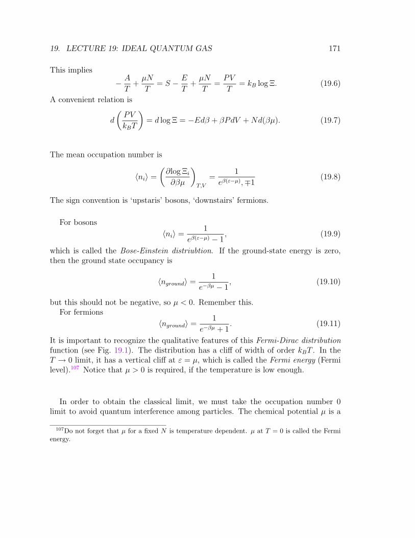
19. LECTURE 19: IDEAL QUANTUM GAS 171
This implies
− A
T+µN
T= S − E
T+µN
T=PV
T= kB log Ξ. (19.6)
A convenient relation is
d
(PV
kBT
)= d log Ξ = −Edβ + βPdV +Nd(βµ). (19.7)
The mean occupation number is
〈ni〉 =
(∂log Ξi
∂βµ
)T,V
=1
eβ(ε−µ),∓1(19.8)
The sign convention is ‘upstaris’ bosons, ‘downstairs’ fermions.
For bosons
〈ni〉 =1
eβ(ε−µ) − 1, (19.9)
which is called the Bose-Einstein distriubtion. If the ground-state energy is zero,then the ground state occupancy is
〈nground〉 =1
e−βµ − 1, (19.10)
but this should not be negative, so µ < 0. Remember this.For fermions
〈nground〉 =1
e−βµ + 1. (19.11)
It is important to recognize the qualitative features of this Fermi-Dirac distributionfunction (see Fig. 19.1). The distribution has a cliff of width of order kBT . In theT → 0 limit, it has a vertical cliff at ε = µ, which is called the Fermi energy (Fermilevel).107 Notice that µ > 0 is required, if the temperature is low enough.
In order to obtain the classical limit, we must take the occupation number 0limit to avoid quantum interference among particles. The chemical potential µ is a
107Do not forget that µ for a fixed N is temperature dependent. µ at T = 0 is called the Fermienergy.
172 CONTENTS
0
1/2
1
expected
occupation
number
μ ε
k TB
symmetric around this point
Figure 19.1: The cliff has a width of order kBT . µ is called the Fermi potential. The symmetrynoted in the figure is the so-called particle-hole symmetry
measure of the “strength” of the chemostat to push particles into the system. Thus,we must make the chemical potential extremely small: µ −∞.
In this limit both Bose-Einstein (19.10) and Fermi-Dirac distributions (19.11)reduce to the Maxwell-Boltzmann distribution as expected:
〈ni〉 → N e−βεi , (19.12)
where N = eβµ is the normalization constant determined by the total number ofparticles in the system.
Notice that µ → −∞ is far away from the situation where quantum effects areimportant µ ' 0 for bosons and µ > 0 for fermions.
Before going to the equations of state, let us to try to build our intuition. Supposethere are only three one-particle states with energies 0, ε and 3ε, and there are threeparticles. Make a table of all the microstates of the system for bosons and fermions.
ε
3ε
0
4ε 0 ε 3ε 2ε 4ε 3ε 5ε 7ε 9εtotal energy 6ε
Figure 19.2: identical particles in three states; fermion (leftmost) and boson cases.
Fermions first:
microstate 0 ε 3ε total energy1 1 1 1 4ε
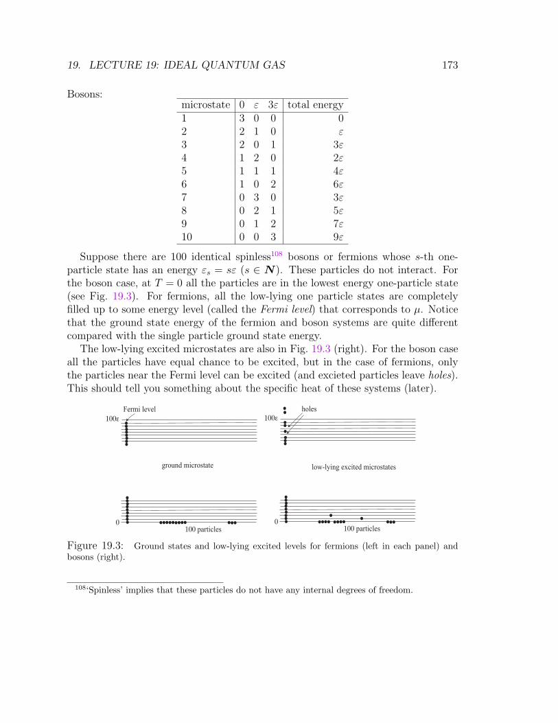
19. LECTURE 19: IDEAL QUANTUM GAS 173
Bosons:microstate 0 ε 3ε total energy1 3 0 0 02 2 1 0 ε3 2 0 1 3ε4 1 2 0 2ε5 1 1 1 4ε6 1 0 2 6ε7 0 3 0 3ε8 0 2 1 5ε9 0 1 2 7ε10 0 0 3 9ε
Suppose there are 100 identical spinless108 bosons or fermions whose s-th one-particle state has an energy εs = sε (s ∈ N ). These particles do not interact. Forthe boson case, at T = 0 all the particles are in the lowest energy one-particle state(see Fig. 19.3). For fermions, all the low-lying one particle states are completelyfilled up to some energy level (called the Fermi level) that corresponds to µ. Noticethat the ground state energy of the fermion and boson systems are quite differentcompared with the single particle ground state energy.
The low-lying excited microstates are also in Fig. 19.3 (right). For the boson caseall the particles have equal chance to be excited, but in the case of fermions, onlythe particles near the Fermi level can be excited (and excieted particles leave holes).This should tell you something about the specific heat of these systems (later).
100ε
0100 particles
100ε
0100 particles
low-lying excited microstatesground microstate
Fermi level holes
Figure 19.3: Ground states and low-lying excited levels for fermions (left in each panel) andbosons (right).
108‘Spinless’ implies that these particles do not have any internal degrees of freedom.
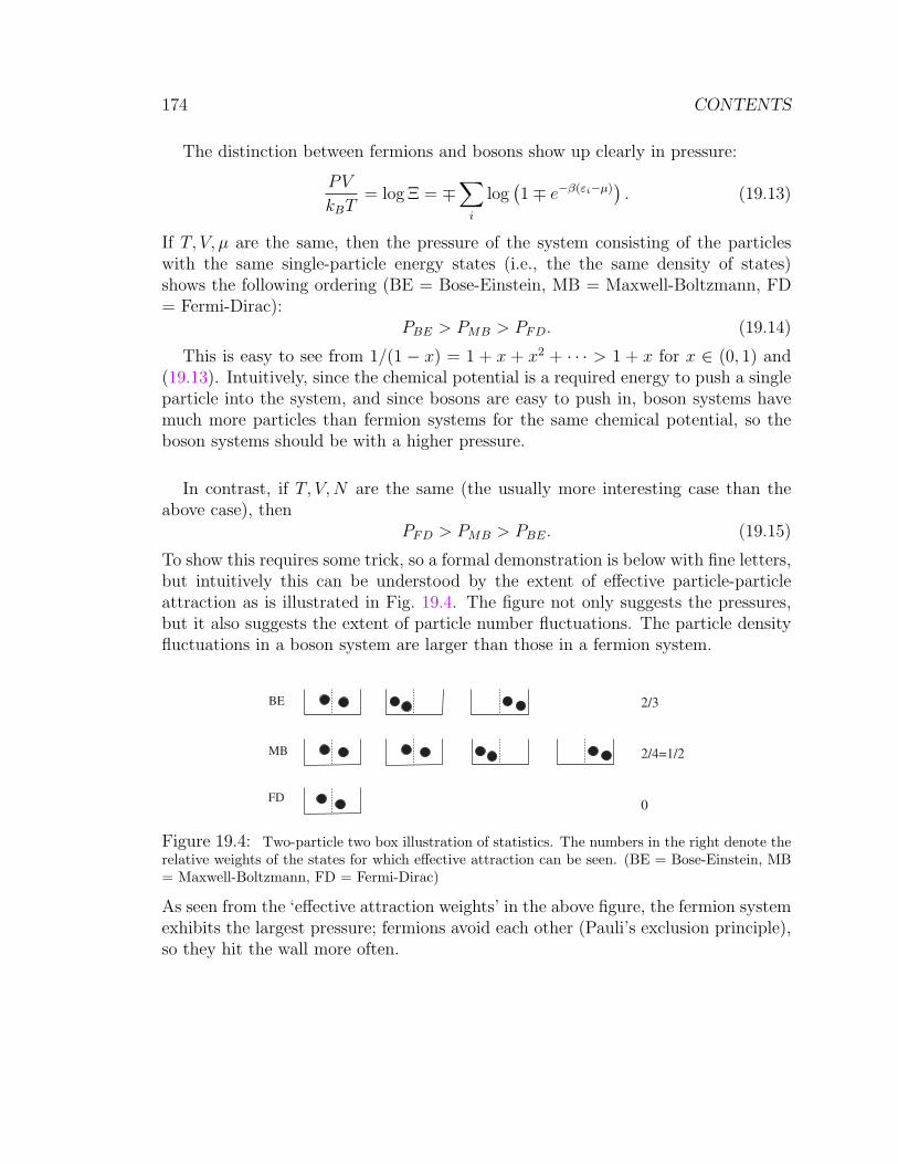
174 CONTENTS
The distinction between fermions and bosons show up clearly in pressure:
PV
kBT= log Ξ = ∓
∑i
log(1∓ e−β(εi−µ)
). (19.13)
If T, V, µ are the same, then the pressure of the system consisting of the particleswith the same single-particle energy states (i.e., the the same density of states)shows the following ordering (BE = Bose-Einstein, MB = Maxwell-Boltzmann, FD= Fermi-Dirac):
PBE > PMB > PFD. (19.14)
This is easy to see from 1/(1 − x) = 1 + x + x2 + · · · > 1 + x for x ∈ (0, 1) and(19.13). Intuitively, since the chemical potential is a required energy to push a singleparticle into the system, and since bosons are easy to push in, boson systems havemuch more particles than fermion systems for the same chemical potential, so theboson systems should be with a higher pressure.
In contrast, if T, V,N are the same (the usually more interesting case than theabove case), then
PFD > PMB > PBE. (19.15)
To show this requires some trick, so a formal demonstration is below with fine letters,but intuitively this can be understood by the extent of effective particle-particleattraction as is illustrated in Fig. 19.4. The figure not only suggests the pressures,but it also suggests the extent of particle number fluctuations. The particle densityfluctuations in a boson system are larger than those in a fermion system.
BE
FD
MB
2/3
2/4=1/2
0
Figure 19.4: Two-particle two box illustration of statistics. The numbers in the right denote therelative weights of the states for which effective attraction can be seen. (BE = Bose-Einstein, MB= Maxwell-Boltzmann, FD = Fermi-Dirac)
As seen from the ‘effective attraction weights’ in the above figure, the fermion systemexhibits the largest pressure; fermions avoid each other (Pauli’s exclusion principle),so they hit the wall more often.

19. LECTURE 19: IDEAL QUANTUM GAS 175
may be demonstrated as follows: Classically, PV = NkBT , so we wish to demonstrate (N and 〈N〉need not be distinguished, since we consider macrosystems)
log ΞFD > 〈N〉 > log ΞBE . (19.16)
Let us see the first inequality:109 Writing xj = e−β(εj−µ), we have
log ΞFD − 〈N〉 =∑
j
[log(1 + xj)−
xj
1 + xj
], (19.17)
where xj = e−β(εj−µ). We are done, because for x > 0110
log(1 + x)− x
1 + x> 0. (19.18)
Similarly, we can prove the second inequality in (19.16).
Let Dt(ε) denote the number of single particle states whose energy is betweenε and ε + dε. This quantity is called the one-particle state density (or density ofstates of one-particle system). If we know this, the pressure (19.13) can be rewrittenas
PV = ∓kBT
∫dεDt(ε) log
(1∓ e−β(ε−µ)
). (19.19)
We know for a classical ideal gas
PV =2
3E, (19.20)
where E is the internal energy. Miraculously, this is true for non-interacting fermionsand bosons (and their mixtures as well). The formulas for PV and E are quitedifferent from the classical case. Here,
E =
∫dεDt(ε)ε〈n(ε)〉 =
∫dεDt(ε)
ε
eβ(ε−µ) ∓ 1. (19.21)
To demonstrate this, we need Dt(ε). I explain a quick way to derive the formulaappropriate in a statistical mechanics course. We count the number of microscopicstates for a single particle up to some energy ε:
1
h3
∫q∈V
dq
∫|p|<
√2mε
dp =
∫ ε
0
dεDt(ε), (19.22)
109The reader might wonder why we cannot use ΞMB to demonstrate the formula; the reasonis that µ in this grand partition function and that in ΞFD or ΞBE are distinct. Remember thatwe keep N ; inevitably µ depends on statistics, so we cannot easily compare the Boltzmann factoreβ(ε−µ) in each term.
110Consider the derivatives.
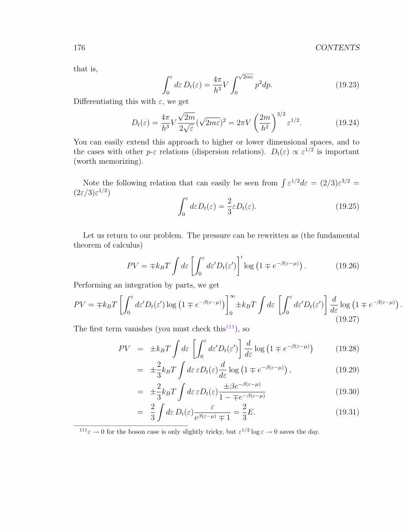
176 CONTENTS
that is, ∫ ε
0
dεDt(ε) =4π
h3V
∫ √2mε
0
p2dp. (19.23)
Differentiating this with ε, we get
Dt(ε) =4π
h3V
√2m
2√ε
(√
2mε)2 = 2πV
(2m
h2
)3/2
ε1/2. (19.24)
You can easily extend this approach to higher or lower dimensional spaces, and tothe cases with other p-ε relations (dispersion relations). Dt(ε) ∝ ε1/2 is important(worth memorizing).
Note the following relation that can easily be seen from∫ε1/2dε = (2/3)ε3/2 =
(2ε/3)ε1/2) ∫ ε
0
dεDt(ε) =2
3εDt(ε). (19.25)
Let us return to our problem. The pressure can be rewritten as (the fundamentaltheorem of calculus)
PV = ∓kBT
∫dε
[∫ ε
0
dε′Dt(ε′)
]′log(1∓ e−β(ε−µ)
). (19.26)
Performing an integration by parts, we get
PV = ∓kBT
[∫ ε
0
dε′Dt(ε′) log
(1∓ e−β(ε−µ)
)]∞0
±kBT
∫dε
[∫ ε
0
dε′Dt(ε′)
]d
dεlog(1∓ e−β(ε−µ)
).
(19.27)The first term vanishes (you must check this111), so
PV = ±kBT
∫dε
[∫ ε
0
dε′Dt(ε′)
]d
dεlog(1∓ e−β(ε−µ)
)(19.28)
= ±2
3kBT
∫dε εDt(ε)
d
dεlog(1∓ e−β(ε−µ)
), (19.29)
= ±2
3kBT
∫dε εDt(ε)
±βe−β(ε−µ)
1−∓e−β(ε−µ)(19.30)
=2
3
∫dεDt(ε)
ε
eβ(ε−µ) ∓ 1=
2
3E. (19.31)
111ε→ 0 for the boson case is only slightly tricky, but ε1/2 log ε→ 0 saves the day.
19. LECTURE 19: IDEAL QUANTUM GAS 177
Now, a bomb making question. There is an isolated metal container of volumeV and energy E with N fermions. These bosons are adiabatically converted intobosons. Can we use this mechanism to make a bomb? Notice that since E and Vare unchanged, the pressure does not change.
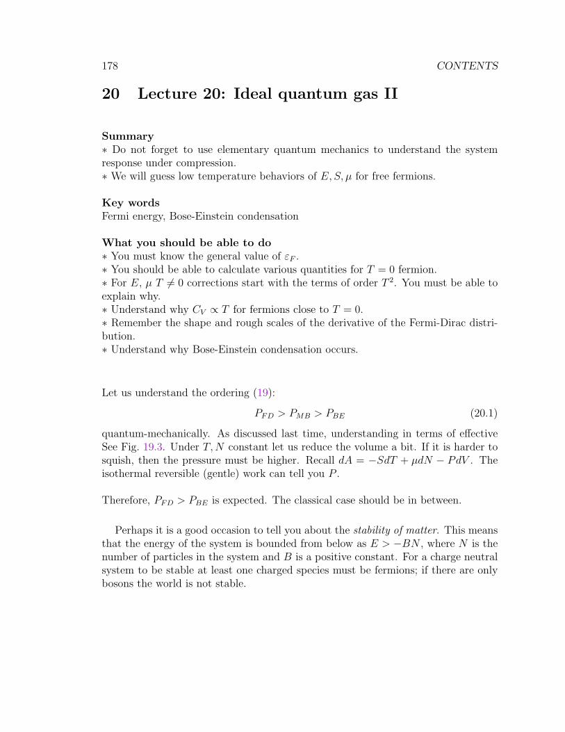
178 CONTENTS
20 Lecture 20: Ideal quantum gas II
Summary∗ Do not forget to use elementary quantum mechanics to understand the systemresponse under compression.∗ We will guess low temperature behaviors of E, S, µ for free fermions.
Key wordsFermi energy, Bose-Einstein condensation
What you should be able to do∗ You must know the general value of εF .∗ You should be able to calculate various quantities for T = 0 fermion.∗ For E, µ T 6= 0 corrections start with the terms of order T 2. You must be able toexplain why.∗ Understand why CV ∝ T for fermions close to T = 0.∗ Remember the shape and rough scales of the derivative of the Fermi-Dirac distri-bution.∗ Understand why Bose-Einstein condensation occurs.
Let us understand the ordering (19):
PFD > PMB > PBE (20.1)
quantum-mechanically. As discussed last time, understanding in terms of effectiveSee Fig. 19.3. Under T,N constant let us reduce the volume a bit. If it is harder tosquish, then the pressure must be higher. Recall dA = −SdT + µdN − PdV . Theisothermal reversible (gentle) work can tell you P .
Therefore, PFD > PBE is expected. The classical case should be in between.
Perhaps it is a good occasion to tell you about the stability of matter. This meansthat the energy of the system is bounded from below as E > −BN , where N is thenumber of particles in the system and B is a positive constant. For a charge neutralsystem to be stable at least one charged species must be fermions; if there are onlybosons the world is not stable.
20. LECTURE 20: IDEAL QUANTUM GAS II 179
Figure 20.1: If the box is compressed, the one-particle energy level spacings increase. Forfermions, the particles tend to move up with the levels because of the Pauli principle, so moreenergy is needed to compress. For bosons, this does not happen. Actually, the ground state actsas a ‘pressure absorber.’
As an application of the Fermi-Dirac distribution, let us consider a free electrongas. Electrons are negatively charged particles, so that the Coulomb interactionamong them is very strong. However, in a metal, the positive charges on the latticeneutralize the total charge, and due to the screening effect even the charge densityfluctuations do not interact strongly. Thus, the free electron model of metals is atleast a good “zeroth order” model of real metals.
Thanks to the ensemble equivalence we can apply the grand canonical scheme toa piece of metal. However, we must choose the chemical potential properly to mimicthe constant particle number N (i.e., density). The total number of particles mustbe
N =∑
i
〈ni〉. (20.2)
The sum is over all the different one particle states of the free electron. The stateof a free electron is completely fixed by its spin (up or down) and its momentum p.There fore, the density of state of free electrons D(ε) = 2Dt(ε), where Dt(ε) is thedensity of states for translational motion (the one already discussed). We alreadyknow the density of states for free particles, but let us repeat this derivation. In thegeneral d-dimensional space, the translational energy density satisfies∫ ε
0
Dt(ε)dε =1
hd
∫V
ddq
∫ε(p)≤ε
ddp (20.3)
If the area (volume) of the d− 1-sphere is written as Sd−1 (S2 = 4π, S1 = 2π), andp(ε) is the magnitude of the momentum given ε (i.e., ε(p(ε)) = ε), then∫ ε
0
D(ε)dε =Sd−1
hdV
∫ p(ε)
0
pd−1dp, (20.4)

180 CONTENTS
so differentiating the both sides with ε, we get
Dt(ε) =Sd−1
hdV p(ε)d−1dp(ε)
dε. (20.5)
In our case p(ε) =√
2mε. In this way, we can derive the density of states for, e.g.,superrelativistic particles with ε = c|p(ε)|.
In this way the density of states D(ε) for the free electron should read
D(ε) = 2Dt(ε) =4πV
h3(2m)3/2ε1/2. (20.6)
Remember the following structure D(ε) = γV ε1/2, where γ is a positive constant.Thus, we have arrived at
N =4πV
h3(2m)3/2
∫ ∞
0
dεε1/2
eβ(ε−µ) + 1, (20.7)
which implicitly fixes µ as a function of T, V and N . We are interested in the systemwith a constant N , so if T changes you must fine-tune µ as a function µ(T ) of T .µ(T ) is determined by solving (20.7). We will look at the beginning step of thisdetermination below, but will not work it out.
At T = 0, the Fermi-Dirac distribution is a step function:
〈n(ε)〉 = θ(εF − ε), (20.8)
where εF = µ is the Fermi energy. Therefore, it is easy to explicitly compute theintegral in (20.7) to get
N =4πV
h3(2m)3/2 2
3ε3/2F , (20.9)
(notice N = (2/3)γV µ(0)3/2.)
εF =h2
2m
(3N
8πV
)2/3
= µ(0). (20.10)
For ordinary metals, εF is of the order of a few eV112 (for copper 7.00 eV, for gold5.90 eV). This kinetic energy corresponds to a speed of electrons of order 1% the
112Remember that 1 eV corresponds to 11604.505kB , that is, about 104 K. The surface temper-ature of the sun is about 6000 K.
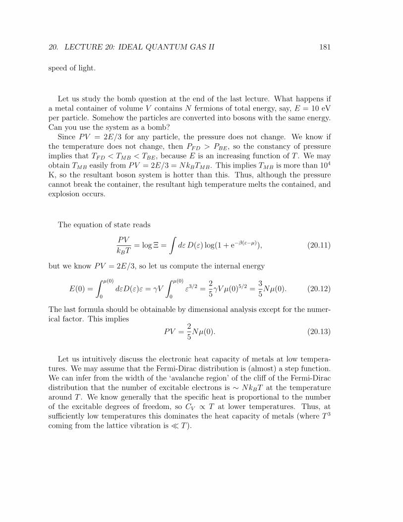
20. LECTURE 20: IDEAL QUANTUM GAS II 181
speed of light.
Let us study the bomb question at the end of the last lecture. What happens ifa metal container of volume V contains N fermions of total energy, say, E = 10 eVper particle. Somehow the particles are converted into bosons with the same energy.Can you use the system as a bomb?
Since PV = 2E/3 for any particle, the pressure does not change. We know ifthe temperature does not change, then PFD > PBE, so the constancy of pressureimplies that TFD < TMB < TBE, because E is an increasing function of T . We mayobtain TMB easily from PV = 2E/3 = NkBTMB. This implies TMB is more than 104
K, so the resultant boson system is hotter than this. Thus, although the pressurecannot break the container, the resultant high temperature melts the contained, andexplosion occurs.
The equation of state reads
PV
kBT= log Ξ =
∫dεD(ε) log(1 + e−β(ε−µ)), (20.11)
but we know PV = 2E/3, so let us compute the internal energy
E(0) =
∫ µ(0)
0
dεD(ε)ε = γV
∫ µ(0)
0
ε3/2 =2
5γV µ(0)5/2 =
3
5Nµ(0). (20.12)
The last formula should be obtainable by dimensional analysis except for the numer-ical factor. This implies
PV =2
5Nµ(0). (20.13)
Let us intuitively discuss the electronic heat capacity of metals at low tempera-tures. We may assume that the Fermi-Dirac distribution is (almost) a step function.We can infer from the width of the ‘avalanche region’ of the cliff of the Fermi-Diracdistribution that the number of excitable electrons is ∼ NkBT at the temperaturearound T . We know generally that the specific heat is proportional to the numberof the excitable degrees of freedom, so CV ∝ T at lower temperatures. Thus, atsufficiently low temperatures this dominates the heat capacity of metals (where T 3
coming from the lattice vibration is T ).
182 CONTENTS
To get this result more quantitatively, we need a way to estimate the contributionof the cliff width. Let us look at the formula for N :
N =
∫ ∞
0
D(ε)1
eβ(ε−µ) − 1(20.14)
Since the FD distribution is almost a step function, its derivative must be sharparound ε = µ:
0_5kT 5kT 10kT10kT_ε _
0.1
0.2
0.3
kT
df
εε
dε
dε
__
μFigure 20.2: The derivative of the Fermi distribution. Its width is about 5kBT . and the heightis β/4.
Let f(ε) = 1/(eβ(ε−µ) − 1). Since we know −f ′(ε) is concentrated sharply aroundε = µ (Fig. 20.2), we wish to use this:∫ ∞
0
[∫ ε
0
D(ε′)dε′]′f(ε)dε =
∫ ε
0
D(ε′)dε′f(ε)
∣∣∣∣∞ε=0
−∫ ∞
0
dε
[∫ ε
0
D(ε′)dε′]f ′(ε)
= −∫ ∞
0
dε
[∫ ε
0
D(ε′)dε′]f ′(ε). (20.15)
Now, f ′ is localized around µ we may expand as follows:
−∫ ∞
0
[∫ µ
0
D(ε′)dε′ +D(µ)(ε− µ) +1
2D′(µ)(ε− µ)2 + · · ·
]f ′(ε)dε
=
∫ µ
0
D(ε′)dε′ − 1
2D′(µ)
∫ ∞
0
(ε− µ)2f ′(ε)dε+ · · · . (20.16)
Detailed calculation is not given here, but it is clear that the correction is of orderT 2; the integral has the dimension of energy squares, so it must be proportional to(kBT )2. If we wish to compute E in the above calculation D is replaced by εD, butthe expansion method is exactly the same, so the correction term is proportional to
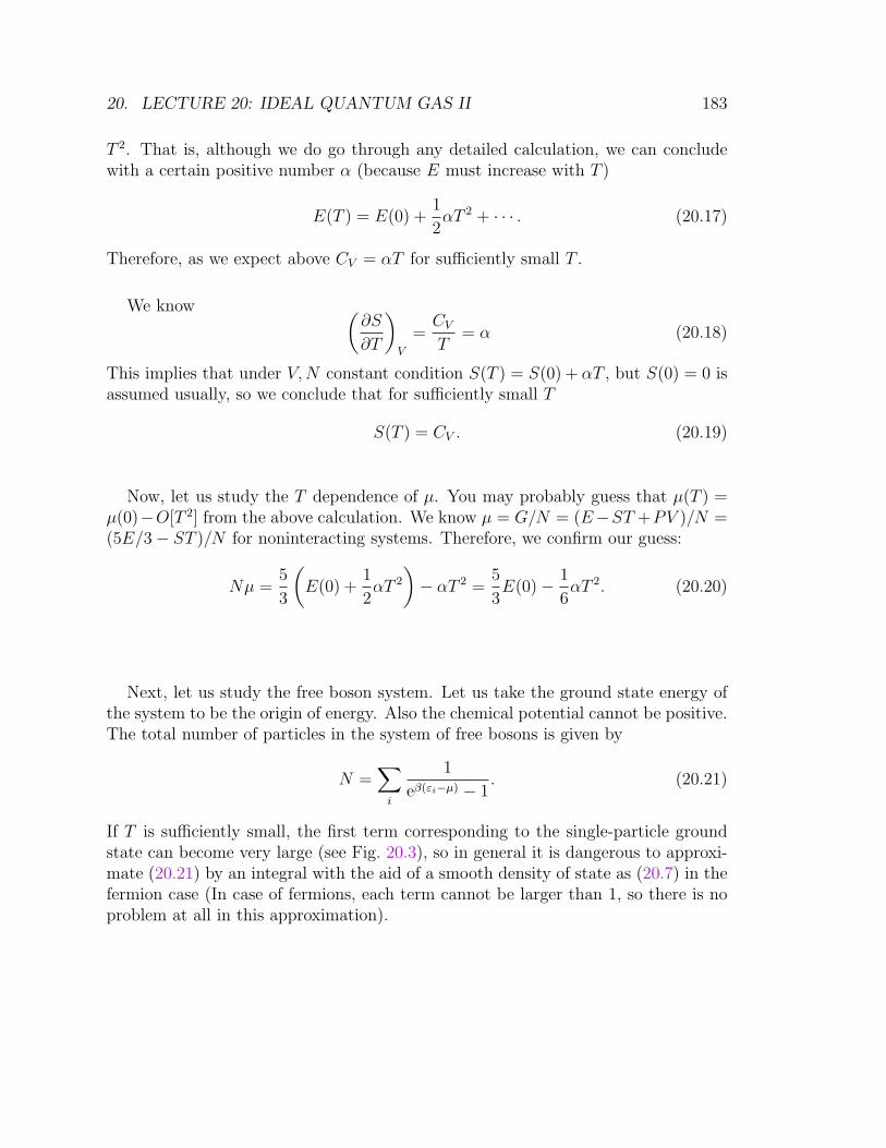
20. LECTURE 20: IDEAL QUANTUM GAS II 183
T 2. That is, although we do go through any detailed calculation, we can concludewith a certain positive number α (because E must increase with T )
E(T ) = E(0) +1
2αT 2 + · · · . (20.17)
Therefore, as we expect above CV = αT for sufficiently small T .
We know (∂S
∂T
)V
=CV
T= α (20.18)
This implies that under V,N constant condition S(T ) = S(0) + αT , but S(0) = 0 isassumed usually, so we conclude that for sufficiently small T
S(T ) = CV . (20.19)
Now, let us study the T dependence of µ. You may probably guess that µ(T ) =µ(0)−O[T 2] from the above calculation. We know µ = G/N = (E−ST +PV )/N =(5E/3− ST )/N for noninteracting systems. Therefore, we confirm our guess:
Nµ =5
3
(E(0) +
1
2αT 2
)− αT 2 =
5
3E(0)− 1
6αT 2. (20.20)
Next, let us study the free boson system. Let us take the ground state energy ofthe system to be the origin of energy. Also the chemical potential cannot be positive.The total number of particles in the system of free bosons is given by
N =∑
i
1
eβ(εi−µ) − 1. (20.21)
If T is sufficiently small, the first term corresponding to the single-particle groundstate can become very large (see Fig. 20.3), so in general it is dangerous to approxi-mate (20.21) by an integral with the aid of a smooth density of state as (20.7) in thefermion case (In case of fermions, each term cannot be larger than 1, so there is noproblem at all in this approximation).
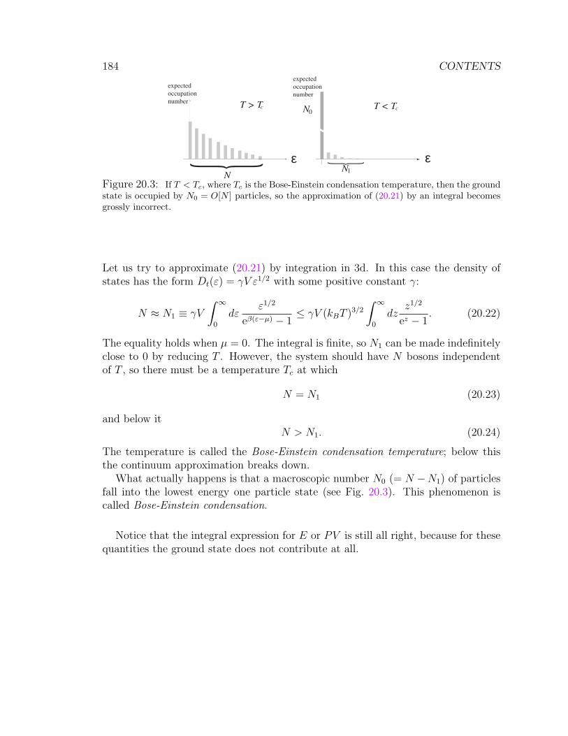
184 CONTENTS
T < T
N
T > Tc c
N
N0
1
εε
expected
occupation
number
expected
occupation
number
Figure 20.3: If T < Tc, where Tc is the Bose-Einstein condensation temperature, then the groundstate is occupied by N0 = O[N ] particles, so the approximation of (20.21) by an integral becomesgrossly incorrect.
Let us try to approximate (20.21) by integration in 3d. In this case the density ofstates has the form Dt(ε) = γV ε1/2 with some positive constant γ:
N ≈ N1 ≡ γV
∫ ∞
0
dεε1/2
eβ(ε−µ) − 1≤ γV (kBT )3/2
∫ ∞
0
dzz1/2
ez − 1. (20.22)
The equality holds when µ = 0. The integral is finite, so N1 can be made indefinitelyclose to 0 by reducing T . However, the system should have N bosons independentof T , so there must be a temperature Tc at which
N = N1 (20.23)
and below itN > N1. (20.24)
The temperature is called the Bose-Einstein condensation temperature; below thisthe continuum approximation breaks down.
What actually happens is that a macroscopic number N0 (= N −N1) of particlesfall into the lowest energy one particle state (see Fig. 20.3). This phenomenon iscalled Bose-Einstein condensation.
Notice that the integral expression for E or PV is still all right, because for thesequantities the ground state does not contribute at all.
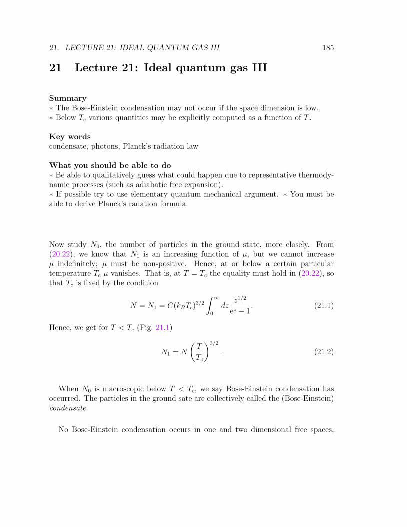
21. LECTURE 21: IDEAL QUANTUM GAS III 185
21 Lecture 21: Ideal quantum gas III
Summary∗ The Bose-Einstein condensation may not occur if the space dimension is low.∗ Below Tc various quantities may be explicitly computed as a function of T .
Key wordscondensate, photons, Planck’s radiation law
What you should be able to do∗ Be able to qualitatively guess what could happen due to representative thermody-namic processes (such as adiabatic free expansion).∗ If possible try to use elementary quantum mechanical argument. ∗ You must beable to derive Planck’s radation formula.
Now study N0, the number of particles in the ground state, more closely. From(20.22), we know that N1 is an increasing function of µ, but we cannot increaseµ indefinitely; µ must be non-positive. Hence, at or below a certain particulartemperature Tc µ vanishes. That is, at T = Tc the equality must hold in (20.22), sothat Tc is fixed by the condition
N = N1 = C(kBTc)3/2
∫ ∞
0
dzz1/2
ez − 1. (21.1)
Hence, we get for T < Tc (Fig. 21.1)
N1 = N
(T
Tc
)3/2
. (21.2)
When N0 is macroscopic below T < Tc, we say Bose-Einstein condensation hasoccurred. The particles in the ground sate are collectively called the (Bose-Einstein)condensate.
No Bose-Einstein condensation occurs in one and two dimensional free spaces,
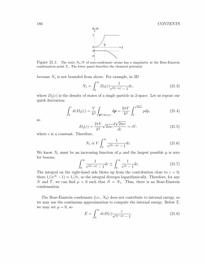
186 CONTENTS
T
N /N
Tc0
1
1
μ0
Figure 21.1: The ratio N1/N of non-condensate atoms has a singularity at the Bose-Einsteincondensation point Tc. The lower panel describes the chemical potential.
because N1 is not bounded from above. For example, in 2D
N1 =
∫ ∞
0
D2(ε)1
eβ(ε−µ) − 1dε, (21.3)
where D2(ε) is the density of states of a single particle in 2-space. Let us repeat ourquick derivation: ∫ ε
0
dεD2(ε) =V
h2
∫p2/2m≤ε
dp =2πV
h2
∫ √2mε
0
pdp, (21.4)
so
D2(ε) =2πV
h2
√2mε
d√
2mε
dε= cV, (21.5)
where c is a constant. Therefore,
N1 ∝ V
∫ ∞
0
1
eβ(ε−µ) − 1dε. (21.6)
We know N1 must be an increasing function of µ and the largest possible µ is zerofor bosons, ∫ ∞
0
1
eβ(ε−µ) − 1dε ≤
∫ ∞
0
1
eβε − 1dε. (21.7)
The integral on the right-hand side blows up from the contribution close to ε = 0;there 1/(eβε− 1) ' 1/βε, so the integral diverges logarithmically. Therefore, for anyN and T , we can find µ < 0 such that N = N1. Thus, there is no Bose-Einsteincondensation.
The Bose-Einstein condensate (i.e., N0) does not contribute to internal energy, sowe may use the continuum approximation to compute the internal energy. Below Tc
we may set µ = 0, so
E =
∫ ∞
0
dεD(ε)ε
eβ(ε−µ) − 1. (21.8)
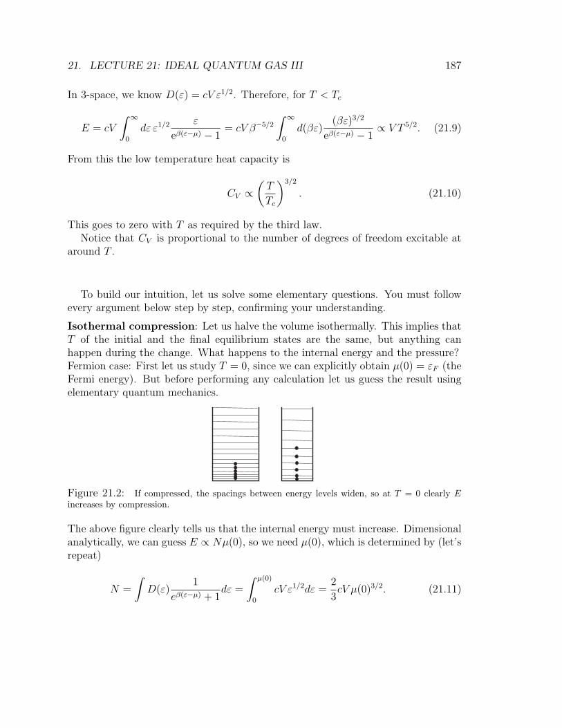
21. LECTURE 21: IDEAL QUANTUM GAS III 187
In 3-space, we know D(ε) = cV ε1/2. Therefore, for T < Tc
E = cV
∫ ∞
0
dε ε1/2 ε
eβ(ε−µ) − 1= cV β−5/2
∫ ∞
0
d(βε)(βε)3/2
eβ(ε−µ) − 1∝ V T 5/2. (21.9)
From this the low temperature heat capacity is
CV ∝(T
Tc
)3/2
. (21.10)
This goes to zero with T as required by the third law.Notice that CV is proportional to the number of degrees of freedom excitable at
around T .
To build our intuition, let us solve some elementary questions. You must followevery argument below step by step, confirming your understanding.
Isothermal compression: Let us halve the volume isothermally. This implies thatT of the initial and the final equilibrium states are the same, but anything canhappen during the change. What happens to the internal energy and the pressure?Fermion case: First let us study T = 0, since we can explicitly obtain µ(0) = εF (theFermi energy). But before performing any calculation let us guess the result usingelementary quantum mechanics.
Figure 21.2: If compressed, the spacings between energy levels widen, so at T = 0 clearly Eincreases by compression.
The above figure clearly tells us that the internal energy must increase. Dimensionalanalytically, we can guess E ∝ Nµ(0), so we need µ(0), which is determined by (let’srepeat)
N =
∫D(ε)
1
eβ(ε−µ) + 1dε =
∫ µ(0)
0
cV ε1/2dε =2
3cV µ(0)3/2. (21.11)
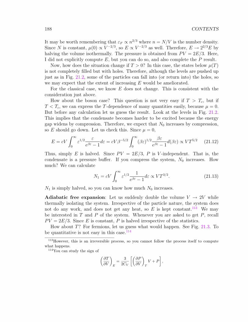
188 CONTENTS
It may be worth remembering that εF ∝ n2/3 where n = N/V is the number density.Since N is constant, µ(0) ∝ V −2/3, so E ∝ V −2/3 as well. Therefore, E → 22/3E byhalving the volume isothermally. The pressure is obtained from PV = 2E/3. Here,I did not explicitly compute E, but you can do so, and also complete the P result.
Now, how does the situation change if T > 0? In this case, the states below µ(T )is not completely filled but with holes. Therefore, although the levels are pushed upjust as in Fig. 21.2, some of the particles can fall into (or return into) the holes, sowe may expect that the extent of increasing E would be ameliorated.
For the classical case, we know E does not change. This is consistent with theconsideration just above.
How about the boson case? This question is not very easy if T > Tc, but ifT < Tc, we can express the T -dependence of many quantities easily, because µ = 0.But before any calculation let us guess the result. Look at the levels in Fig. 21.2.This implies that the condensate becomes harder to be excited because the energygap widens by compression. Therefore, we expect that N0 increases by compression,so E should go down. Let us check this. Since µ = 0,
E = cV
∫ ∞
0
ε1/2 ε
eβε − 1dε = cV β−5/2
∫ ∞
0
(βε)1/2 βε
eβε − 1d(βε) ∝ V T 5/2 (21.12)
Thus, simply E is halved. Since PV = 2E/3, P is V -independent. That is, thecondensate is a pressure buffer. If you compress the system, N0 increases. Howmuch? We can calculate
N1 = cV
∫ ∞
0
ε1/2 1
eβε − 1dε ∝ V T 3/2. (21.13)
N1 is simply halved, so you can know how much N0 increases.
Adiabatic free expansion: Let us suddenly double the volume V → 2V whilethermally isolating the system. Irrespective of the particle nature, the system doesnot do any work, and does not get any heat, so E is kept constant.113 We maybe interested in T and P of the system. Whenever you are asked to get P , recallPV = 2E/3. Since E is constant, P is halved irrespective of the statistics.
How about T? For fermions, let us guess what would happen. See Fig. 21.3. Tobe quantitative is not easy in this case.114
113However, this is an irreversible process, so you cannot follow the process itself to computewhat happens.
114You can study the sign of (∂T
∂V
)E
=3
2CV
[(∂P
∂V
)T
V + P
],
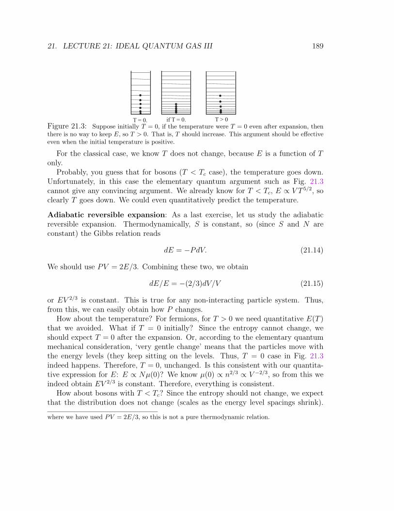
21. LECTURE 21: IDEAL QUANTUM GAS III 189
if T = 0.T = 0. T > 0
Figure 21.3: Suppose initially T = 0, if the temperature were T = 0 even after expansion, thenthere is no way to keep E, so T > 0. That is, T should increase. This argument should be effectiveeven when the initial temperature is positive.
For the classical case, we know T does not change, because E is a function of Tonly.
Probably, you guess that for bosons (T < Tc case), the temperature goes down.Unfortunately, in this case the elementary quantum argument such as Fig. 21.3cannot give any convincing argument. We already know for T < Tc, E ∝ V T 5/2, soclearly T goes down. We could even quantitatively predict the temperature.
Adiabatic reversible expansion: As a last exercise, let us study the adiabaticreversible expansion. Thermodynamically, S is constant, so (since S and N areconstant) the Gibbs relation reads
dE = −PdV. (21.14)
We should use PV = 2E/3. Combining these two, we obtain
dE/E = −(2/3)dV/V (21.15)
or EV 2/3 is constant. This is true for any non-interacting particle system. Thus,from this, we can easily obtain how P changes.
How about the temperature? For fermions, for T > 0 we need quantitative E(T )that we avoided. What if T = 0 initially? Since the entropy cannot change, weshould expect T = 0 after the expansion. Or, according to the elementary quantummechanical consideration, ‘very gentle change’ means that the particles move withthe energy levels (they keep sitting on the levels. Thus, T = 0 case in Fig. 21.3indeed happens. Therefore, T = 0, unchanged. Is this consistent with our quantita-tive expression for E: E ∝ Nµ(0)? We know µ(0) ∝ n2/3 ∝ V −2/3, so from this weindeed obtain EV 2/3 is constant. Therefore, everything is consistent.
How about bosons with T < Tc? Since the entropy should not change, we expectthat the distribution does not change (scales as the energy level spacings shrink).
where we have used PV = 2E/3, so this is not a pure thermodynamic relation.
190 CONTENTS
Therefore, we expect N0 does not change. Of course, the elementary quantum ar-gument tells you the same. Is this correct? Since E ∝ V T 5/2 and EV 2/3 must beconstant, V 5/3T 5/2 or V T 3/2 must be constant. We know N1 ∝ V T 3/2, so indeed N1
is constant.
Photons and phonons are obtained through quantization of the systems that canbe described as a collection of harmonic oscillators.115 Possible energy levels for thei-th mode whose angular frequency is ωi
116 are (n+1/2)~ωi. The canonical partitionfunction of the whole systems is given by
Z(β) =∏
i
(∑ni
e−β(ni+1/2)~ωi
), (21.16)
since no modes interact each other. Here, the product is over all the modes. Thesum in the parentheses gives the canonical partition function for a single harmonicoscillator, which we have already computed. The canonical partition function maybe rewritten as:
Z(β) =∏
i
(e−β~ωi/2
)Ξ(β, 0). (21.17)
Here, we have used the formula
Ξ(β, 0) =∏
i
(∞∑
n=0
e−βn~ωi
), (21.18)
which may be obtained from the definition of the grand partition function by settingεi = ~ωi, and µ = 0. As long as we consider a single system, the total zero-point energy of the system
∑i ~ωi/2 may be ignored by shifting the energy origin.117
115That is, the system whose Hamiltonian is quadratic in canonical coordinates (quantum me-chanically in the corresponding operators).
116A system with a quadratic Hamiltonian may be described in terms of canonical coordinates(or corresponding operators) that makes the Hamiltonian diagonal. In other words, the systemmay be described as a collection of independent harmonic oscillators. The motion correspondingto each such harmonic oscillator is called a mode. If more than one modes have identical angularfrequencies, modes cannot be uniquely chosen, but this does not cause any problem to us becausepartition functions need the system energies and their degeneracies only.
117However, if the system is deformed or chemical reactions occur, the system zero-point energycan change, so we must go back to the original formula with the total zero-point energy and take intoaccount its contribution. We have already seen this when we computed the chemical equilibriumconstant. Furthermore, for electromagnetic field, the change of the total zero-point energy may beobserved as force. This is the Casimir effect.
21. LECTURE 21: IDEAL QUANTUM GAS III 191
Therefore, the canonical partition function of the system consisting of photons orphonons may be written as ΞBE(β, 0). That is, it is written as the bosonic grandpartition function with a zero chemical potential.
The thermodynamic potential for the system consisting of photons or phononsis the Helmholtz free energy A whose independent variables are T and V , becausethe expected number 〈ni〉 of phonons (photons) of mode i is determined, if thetemperature T and the volume V are given. Notice that we do not have any more‘handle’ like µ to modify the expectation value. Since dA = −SdT − PdV , we haveA = −PV . That is, our observation logZ(β) = log Ξ(β, 0) holds as a thermodynamicrelation for a system that can be described by a collection of harmonic oscillators(as long as we ignore the zero-point energy). Thus, we may conclude that systemsconsisting of phonons or photons can be described consistently by the grand partitionfunction with a zero chemical potential. For example, the pressure of the photon orphonon system can be computed immediately as we see below.
However, do not understand this relation to indicate that the chemical potentialsof photons and phonons are indeed zero; actually they cannot be defined. Therelation is only a mathematical formal relation that can be sometimes useful.
The µ = 0 boson analogy118 tells us that the average number of phonons of aharmonic mode is given by
〈n〉 =1
e+β~ω − 1. (21.19)
The phonon contribution to the internal energy of a system may be computed justas we did for the Debye model. We need the density of states (i.e, phonon spectrum)f(ω). The internal energy of all the phonons is given by
E =∑
modes
〈n(ω)〉~ω =
∫dωf(ω)
~ωe+β~ω − 1
. (21.20)
This is the internal energy without the contribution of zero-point energy. The lattercontribution is a mere constant shifting the origin of energy, so it is thermodynami-cally irrelevant.
118They are bosons. This is all right. What is not correct is the statement that phonons orphotons have chemical potentials. Intuitively speaking, chemical potential may be defined only forparticles you can ‘pick up.’ More precisely speaking, if no charge of some kind (say, electric charge,baryon number) is associated with the particle, its chemical potential is a dubious concept.
192 CONTENTS
Photons are quanta of light or electromagnetic wave. Photons have spin 1, butthey travel at the speed of light, so the z-component of its spin takes only ±1.This corresponds to the polarization vector of light. As with phonons, there is noconstraint on the number of photons. Photons result from quantization of electro-magnetic waves, so mathematically they just behave as phonons. Thus, formally, wemay treat photons as bosons with two internal states and with µ = 0. Hence, thenumber of photons of a given mode reads exactly the same as (21.19).
Let f(ω)dω be the number of modes with angular frequency between ω and ω+dω(the photon spectrum). The internal energy dEω and the number dNω of photons inthis range are given by
dEω = 2f(ω)~ω
e+β~ω − 1dω, (21.21)
dNω = 2f(ω)1
eβ~ω − 1dω. (21.22)
The factor 2 comes from the polarization states.A standard way to obtain the density of states f(ω) is to study the wave equation
governing the electromagnetic waves, but here we use a shortcut. The dispersionrelation for photons is ε = c|p| = ~ω, so∫ ω
0
f(ω′)dω′ =V
h3
∫|p|≤~ω/c
d3p (21.23)
Here, we do not include the factor 2 due to polarization states. Therefore. differen-tiating the above equality, we obtain
f(ω) =4πV
h3
(~ωc
)2 ~c
=V ω2
2π2c3(21.24)
Therefore, the energy density u(T., ω) at temperature T due to the photons with theangular frequencies around ω reads
u(T, ω) =V ω2
π2c3~ω
eβ~ω − 1. (21.25)
This is Planck’s radiation formula.It is important to know some qualitative features of this law (Fig. 21.4).
Planck’s law can explain why the spectrum blue-shifts as temperature increases; thiswas not possible within the classical theory.

21. LECTURE 21: IDEAL QUANTUM GAS III 193
Figure 21.4: Classical electrodynamics gives the Rayleigh-Jeans formula (21.27) (green); thisis the result of equipartition of energy and due to many UV modes, the density is not integrable(the total energy diverges). Wien reached (21.28) empirically (red). Planck arrived at his formula(black) originally by interpolation of these two results. Notice that the peak position is proportionalto the temperature.
The total energy density u(T ) = E/V of a radiation field is obtained by integra-tion:
u(T ) =
∫ ∞
0
dω u(T, ω). (21.26)
With Planck’s law (21.25) this is always finite. If the limit ~ → 0 is taken (theclassical limit), we get
u(T, ω) =kBTω
2
π2c3( = 2f(ω)kBT ) , (21.27)
which is the formula obtained by classical physics. Upon integration, the classicallimit gives an infinite u(T ). The reason for this divergence is obviously due to the con-tribution from the high frequency modes. Thus this difficulty is called the ultravioletcatastrophe, which destroyed classical physics. Empirically, Wien proposed
u(T, ω) ' kBT
π2c3ω2e−β~ω. (21.28)
The formula can be obtained from Planck’s law in the limiting case ~ω kBT .
194 CONTENTS
22 Lecture 22: Quantum internal degrees, Fluc-
tuations and response
Summary∗ The Stefan-Boltzmann law can be derived if we know the photn pressur PV = E/3and thermodynamics.∗ The quantization effect of the internal degrees of freedom may not be ignored evenfor classical ideal gas.∗ Fluctuation and susceptibility are closely related (fluctuation-response relation).∗ Einstein’s theory of thermodynamic fluctuation.
Key wordsStefan-Boltzmann relation, internal degreez of freedom, fluctuation-response relation,large deviation rate function, fundamental formula for thermodynamic fluctuations
What you should be able to do∗ Explain CV intuitively (see Fig. 22.1).∗ Explain internal degrees of freedom and be able to sketch the CV -T curve.∗ Explain the major features understanable fluctuation-response relations.
Let us finish the statistical mechanics of back-body radiation. Let us find theequation of state of the radiation field (i.e., the photon pressure). First let us reviewwhat we learned.
We can obtain the density of states with the aid of∫ ε
0
dεD(ε) = 2× V
h34π
∫ ε/c
0
p2dp, (22.1)
where we have used the dispersion relation ε = cp; the factor 2 in front of the RHSis the state multiplicity of photons due to polarization. Thus,
D(ε) =8πV
c3h3ε2. (22.2)
Planck actually wanted the density of state f(ω) in terms of ω. Since ε = ~ω, wehave
f(ω)dω = D(ε)dε ⇒ f(ω) = D(~ω)~.
22. LECTURE 22: QUANTUM INTERNAL DEGREES, FLUCTUATIONS AND RESPONSE195
Therefore,
f(ω) =8πV
c3h3(~ω)2~ =
8πV
c38π3ω2 =
ω2
π2c3V, (22.3)
which is identical to the result we got in the last lecture.Thus, the energy density in [ω, ω + dω) is (notice that our D or f contains the
volume V to study the whole system, so this V must be factored out to obtain thedensity)
u(ω, T ) =ω2
π2c3~ω
eβ~ω − 1. (22.4)
The total energy density E/V at temperature T is
u(T ) =
∫ ∞
0
ω2
π2c3~ω
eβ~ω − 1dω = β−4
∫ ∞
0
(βω)2
π2c3~βω
eβ~ω − 1d(βω). (22.5)
This immediately implies (as seen above)
u(T ) ∝ T 4. (22.6)
which is called the Stefan-Boltzmann law.
Since we know the T 3-law of the phonon low temperature specific heat (the Debyetheory), this should be expected. This is understandable by counting the numberof degrees of freedom (Fig. 22.1). Although we did not calculate the proportionalityconstant, if you follow the above calculation you can get it. This proportionality wasobtained purely thermodynamically by Boltzmann before the advent of quantummechanics. The proportionality constant contains ~, so it was impossible to theo-retically obtain the proportionality constant before Planck (Stefan experimentallyobtained it).
Photons may be treated as ideal bosons with µ = 0,119 so the equation of state isimmediately obtained as
PV
kBT= log Ξ = −
∫dεD(ε) log(1− e−βε). (22.7)
For 3D superrelativistic particles, D(ε) ∝ ε2, so∫ ε
0
dεD(ε) =1
3εD(ε). (22.8)
119If µ = 0, then A = −PV = −kBT log Z.
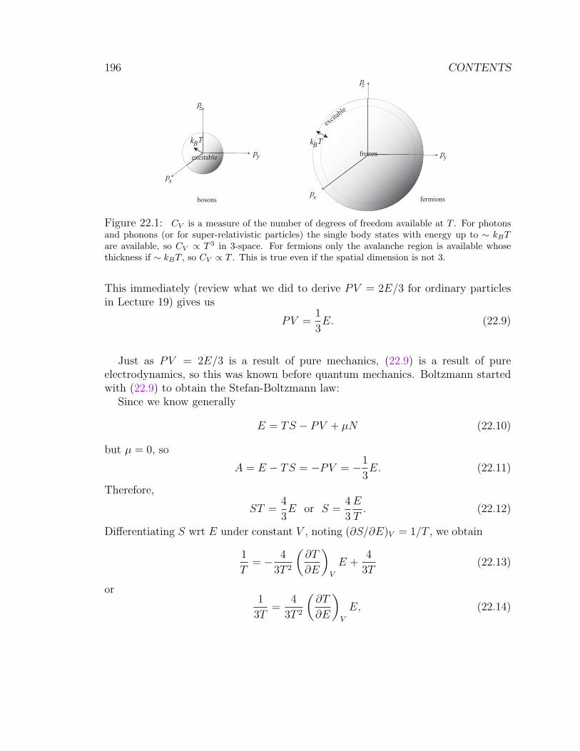
196 CONTENTS
p
p
px
z
y
Bk T
p
p
px
z
y
Bk T
excitable
frozenexcitable
bosons fermions
Figure 22.1: CV is a measure of the number of degrees of freedom available at T . For photonsand phonons (or for super-relativistic particles) the single body states with energy up to ∼ kBTare available, so CV ∝ T 3 in 3-space. For fermions only the avalanche region is available whosethickness if ∼ kBT , so CV ∝ T . This is true even if the spatial dimension is not 3.
This immediately (review what we did to derive PV = 2E/3 for ordinary particlesin Lecture 19) gives us
PV =1
3E. (22.9)
Just as PV = 2E/3 is a result of pure mechanics, (22.9) is a result of pureelectrodynamics, so this was known before quantum mechanics. Boltzmann startedwith (22.9) to obtain the Stefan-Boltzmann law:
Since we know generally
E = TS − PV + µN (22.10)
but µ = 0, so
A = E − TS = −PV = −1
3E. (22.11)
Therefore,
ST =4
3E or S =
4
3
E
T. (22.12)
Differentiating S wrt E under constant V , noting (∂S/∂E)V = 1/T , we obtain
1
T= − 4
3T 2
(∂T
∂E
)V
E +4
3T(22.13)
or1
3T=
4
3T 2
(∂T
∂E
)V
E, (22.14)
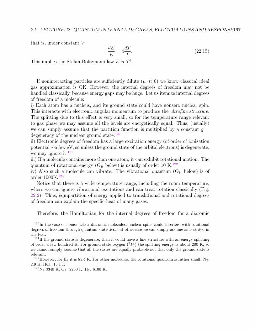
22. LECTURE 22: QUANTUM INTERNAL DEGREES, FLUCTUATIONS AND RESPONSE197
that is, under constant VdE
E= 4
dT
T. (22.15)
This implies the Stefan-Boltzmann law E ∝ T 4.
If noninteracting particles are sufficiently dilute (µ 0) we know classical idealgas approximation is OK. However, the internal degrees of freedom may not behandled classically, because energy gaps may be huge. Let us itemize internal degreesof freedom of a molecule:i) Each atom has a nucleus, and its ground state could have nonzero nuclear spin.This interacts with electronic angular momentum to produce the ultrafine structure.The splitting due to this effect is very small, so for the temperature range relevantto gas phase we may assume all the levels are energetically equal. Thus, (usually)we can simply assume that the partition function is multiplied by a constant g =degeneracy of the nuclear ground state.120
ii) Electronic degrees of freedom has a large excitation energy (of order of ionizationpotential ∼a few eV, so unless the ground state of the orbital electrons) is degenerate,we may ignore it.121
iii) If a molecule contains more than one atom, it can exhibit rotational motion. Thequantum of rotational energy (ΘR below) is usually of order 10 K.122
iv) Also such a molecule can vibrate. The vibrational quantum (ΘV below) is oforder 1000K.123
Notice that there is a wide temperature range, including the room temperature,where we can ignore vibrational excitations and can treat rotation classically (Fig.22.2). Thus, equipartition of energy applied to translational and rotational degreesof freedom can explain the specific heat of many gases.
Therefore, the Hamiltonian for the internal degrees of freedom for a diatomic
120In the case of homonuclear diatomic molecules, nuclear spins could interfere with rotationaldegrees of freedom through quantum statistics, but otherwise we can simply assume as is stated inthe text.
121If the ground state is degenerate, then it could have a fine structure with an energy splittingof order a few hundred K. For ground state oxygen (3P2) the splitting energy is about 200 K, sowe cannot simply assume that all the states are equally probable nor that only the ground slate isrelevant.
122However, for H2 it is 85.4 K. For other molecules, the rotational quantum is rather small: N2:2.9 K; HCl: 15.1 K.
123N2 3340 K; O2: 2260 K; H2: 6100 K.
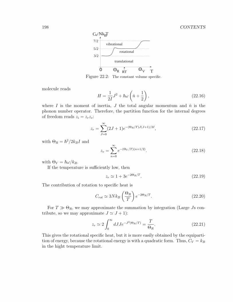
198 CONTENTS
vibrational
rotational
translational
vC /Nk TB
TΘ ΘR V0
3/2
5/2
7/2
RT
Figure 22.2: The constant volume specific.
molecule reads
H =1
2IJ2 + ~ω
(n+
1
2
), (22.16)
where I is the moment of inertia, J the total angular momentum and n is thephonon number operator. Therefore, the partition function for the internal degreesof freedom reads zi = zrzv:
zr =∞∑
J=0
(2J + 1)e−(ΘR/T )J(J+1)/2I , (22.17)
with ΘR = ~2/2kBI and
zv =∞∑
n=0
e−(ΘV /T )(n+1/2). (22.18)
with ΘV = ~ω/kB.If the temperature is sufficiently low, then
zr ' 1 + 3e−2ΘR/T . (22.19)
The contribution of rotation to specific heat is
Crot ' 3NkB
(ΘR
T
)e−2ΘR/T . (22.20)
For T ΘR, we may approximate the summation by integration (Large Js con-tribute, so we may approximate J ' J + 1):
zr ' 2
∫ ∞
0
dJJe−J2(ΘR/T ) =T
ΘR
. (22.21)
This gives the rotational specific heat, but it is more easily obtained by the equiparti-tion of energy, because the rotational energy is with a quadratic form. Thus, CV = kB
in the hight temperature limit.
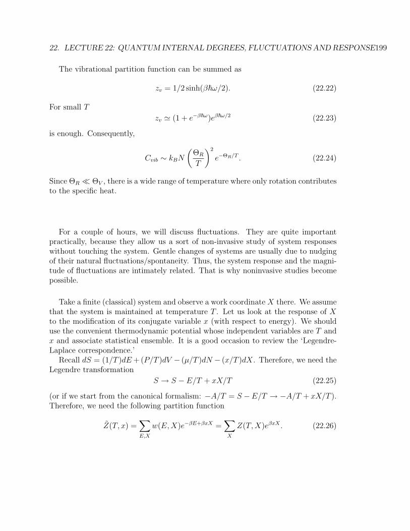
22. LECTURE 22: QUANTUM INTERNAL DEGREES, FLUCTUATIONS AND RESPONSE199
The vibrational partition function can be summed as
zv = 1/2 sinh(β~ω/2). (22.22)
For small T
zv ' (1 + e−β~ω)eβ~ω/2 (22.23)
is enough. Consequently,
Cvib ∼ kBN
(ΘR
T
)2
e−ΘR/T . (22.24)
Since ΘR ΘV , there is a wide range of temperature where only rotation contributesto the specific heat.
For a couple of hours, we will discuss fluctuations. They are quite importantpractically, because they allow us a sort of non-invasive study of system responseswithout touching the system. Gentle changes of systems are usually due to nudgingof their natural fluctuations/spontaneity. Thus, the system response and the magni-tude of fluctuations are intimately related. That is why noninvasive studies becomepossible.
Take a finite (classical) system and observe a work coordinateX there. We assumethat the system is maintained at temperature T . Let us look at the response of Xto the modification of its conjugate variable x (with respect to energy). We shoulduse the convenient thermodynamic potential whose independent variables are T andx and associate statistical ensemble. It is a good occasion to review the ‘Legendre-Laplace correspondence.’
Recall dS = (1/T )dE+(P/T )dV − (µ/T )dN − (x/T )dX. Therefore, we need theLegendre transformation
S → S − E/T + xX/T (22.25)
(or if we start from the canonical formalism: −A/T = S −E/T → −A/T + xX/T ).Therefore, we need the following partition function
Z(T, x) =∑E,X
w(E,X)e−βE+βxX =∑X
Z(T,X)eβxX . (22.26)
200 CONTENTS
Here,∑
implies summation or integration. Z is a generalized canonical parti-tion function (compare this with the grand partition function) and amy be writtenas
Z(T, x) = Tre−βH+βxX , (22.27)
where X is the microscopic description of the work coordinate X (= 〈X〉). Thefundamental relation is
S − E
T+xX
T= kB log Z(T, x). (22.28)
Since d(S − E/T + xX/T ) = −Ed(1/T )− (P/T )dV +Xd(x/T ), we have
d log Z(β, x) = −Edβ − βPdV +Xd(βx). (22.29)
The susceptibility χ = (∂X/∂x)T,V of the responseX to the change of x reads
χ = β∂2 log Z
∂(βx)2. (22.30)
X =∂log Z
∂βx=
1
Z
∑Xe−βH+βxX . (22.31)
Let’s differentiate this once more:
χ = β∂X
∂βx= − 1
Z2
(∑Xe−βH+βxX
)2
+1
Z
∑X2e−βH+βxX . (22.32)
That is,
= β(〈X2〉 − 〈X〉2
)= β〈δX2〉 ≥ 0, (22.33)
where δX = X − 〈X〉. This is the fluctuation-response relation.
We can make three important observations from the fluctuation-response relation(22.33):(i) The ‘ease’ of response results from ‘large’ fluctuations. Notice that χ describesthe response to an external perturbation, but the variance of X is due to spontaneousthermal fluctuations. Gentle nudging of the system (reversible change) must respectthe spontaneity of the system.(ii) Since X is extensive and x is intensive, χ must be extensive (proportional to the
22. LECTURE 22: QUANTUM INTERNAL DEGREES, FLUCTUATIONS AND RESPONSE201
number of particles there, N). Therefore, δX = O[√N ].124
(iii) χ cannot be negative. This is the manifestation of the stability of the equilibriumstate (free energy minimum) as we will see in more detail later.
Can you guess the general formula when there are many variables?
Thus, we have realized that studying fluctuation is quite important; it couldbe a non-invasive method to study the system response. The study of fluctuationis a mesoscopic scale study of the system, so it is the study of large deviation.Thus, if we know the rate function I, we are done. Einstein gave I for equilibriumfluctuations.
So far we have studied very large systems (thermodynamic limit). There, the law oflarge numbers reigns: for any ε > 0
P
(∣∣∣∣ 1V X(V )− 〈X〉∣∣∣∣ > ε
)→ 0 (22.34)
in the V → ∞ limit, where V is the volume of the domain we observe, X(V ) isthe observed result there,125 and 〈X〉 is the equilibrium value.126 If we observe avolume that is not large, then, the probability above is positive. That is, we observefluctuations.
We know such deviations from the law of large numbers can be studied with theaid of the large deviation theory (e.g., Lecture 6):
P
(1
VX(V ) ∼ y
)≈ e−V I(y), (22.35)
where I is the large deviation function (or rate function). If we know I, basically weknow everything we wish to know about fluctuations.
In practice, even if we say the volume we observe is tiny, since we are macroscopicorganisms, the volume is sufficiently large from the microscopic point of view. There-fore, fluctuations should not be very large, and we have only to consider the second
124away from critical points. There, χ can diverge, so nothing can be said from this argument.125If X is extensive, X(V ) is the total amount in V (i.e., X(V )/V is its density). If X is intensive,
then X(V )/V should be interpreted as the average value in the volume V .126If X is extensive, it is the corresponding density; if X is intensive, it is the equilibrium value.
202 CONTENTS
moments to quantify fluctuations.127 That is, we need the quadratic approximationto I, which was provided by Einstein.
Einstein in 1910128 studied the deviation of thermodynamic observables in a smalldomain of a system from their equilibrium values in order to understand criticalfluctuations.129 To obtain the probability of fluctuations, he inverted the Boltzmannprinciple as
w(X) = eS(X)/kB , (22.36)
where X collectively denotes extensive variables. Then, he postulated that thestatistical weight for the value of X deviated from its equilibrium value may alsobe obtained by (22.36). Since we know the statistical weights, we can compute theprobability of observing X as
P (X) =w(X)∑Xw(X)
. (22.37)
The denominator may be replaced with the largest term in the summands, so wemay rewrite the formula as
P (X) ' w(X)w(Xeq)
= e[S(X)−S(Xeq)]/kB = e−|∆S|/kB , (22.38)
where ' implies the equality up to a certain unimportant numerical coefficient, andXeq is the value of X that gives the largest w (maximizes the entropy), that is,the equilibrium value. ∆S = S(X)− S(Xeq) is written as −|∆S| to emphasizethe sign of ∆S (i.e., negative). To the second order
P (δX) ∝ e−|δ2S|/kB . (22.39)
Einstein proposed this as the fundamental formula for small fluctuations in a smallportion of any equilibrium system.
127If the reader remembers theory, she will realize that we are discussing the quadratic approxi-mation of the rate function.
128[This year, Russel and Whitehead started to publish Principia Mathematica (∼1913), theMexican revolution began, Tolstoy died (11/20, 1817∼) Nightingale died.]
129A. Einstein, “Theorie der Opaleszenz von homogenen Flussigkeitsgemischen in der Nahe deskritischen Zustandes,” Ann. Phys., 33, 1275-1298 (1910). [Theory of critical opalescence of homo-geneous fluid mixture near the critical state]. J. D. Jackson, Classical Electrodynamics, 2nd Edition(Wiley, 1975) Sect. 9.7 is a good summary of related topics.
23. LECTURE 23: MESOSCOPIC FLUCTUATIONS; TIME-DEPENDENCE AS WELL203
23 Lecture 23: Mesoscopic fluctuations; time-dependence
as well
Summary∗ How to use Einstein’s thermodynamic fluctuation theory.∗ Onsager theory of linear nonequilibrium phenomena is outlined. Large deviationtheory can unify the theoretical framework.
Key wordsOnsager coefficient, Onsager’s principle, Onsager’s reciprocity relation, Green-Kuborelation.
What you should be able to do∗ You must be able to write down the practical formula governing the fluctuationprobability.∗ It may be a good occasion to be familiar with the multivariate Gaussian distribu-tion.
Thesis Topic: Generalize the Large deviation theoretical unification to quantumcases.
Let us review the fluctuation-response relation
χij =
(∂Xi
∂xj
)xk
= β〈(Xi − 〈Xi〉)(Xj − 〈Xj〉)〉. (23.1)
This implies something about the stability, size of the fluctuation, and general ‘causeof response to external gentle forcing’: it is spontaneous fluctuation in the system.Also, this tells you Maxwell’s relation(
∂Xi
∂xj
)···
=
(∂Xj
∂xi
)···. (23.2)
Since Xx has the dimension of energy, β appears on the RHS.
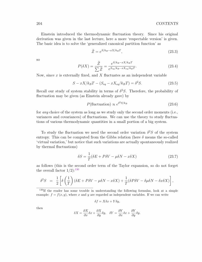
204 CONTENTS
Einstein introduced the thermodynamic fluctuation theory. Since his originalderivation was given in the last lecture, here a more ‘respectable version’ is given.The basic idea is to solve the ‘generalized canonical partition function’ as
Z = eS/kB−xX/kBT , (23.3)
so
P (δX) =Z∑Z
=eS/kB−xX/kBT
eSeq/kB−xXeq/kBT. (23.4)
Now, since x is externally fixed, and X fluctuates as an independent variable
S − xX/kBT − (Seq − xXeq/kBT ) = δ2S. (23.5)
Recall our study of system stability in terms of δ2S. Therefore, the probability offluctuation may be given (as Einstein already gave) by
P (fluctuation) ∝ eδ2S/kB (23.6)
for any choice of the system as long as we study only the second order moments (i.e.,variances and covariances) of fluctuations. We can use the theory to study fluctua-tions of various thermodynamic quantities in a small portion of a big system.
To study the fluctuation we need the second order variation δ2S of the systementropy. This can be computed from the Gibbs relation (here δ means the so-called‘virtual variation,’ but notice that such variations are actually spontaneously realizedby thermal fluctuations)
δS =1
T(δE + PδV − µδN − xδX) (23.7)
as follows (this is the second order term of the Taylor expansion, so do not forgetthe overall factor 1/2):130
δ2S =1
2
[δ
(1
T
)(δE + PδV − µδN − xδX) +
1
T(δPδV − δµδN − δxδX)
],
130If the reader has some trouble in understanding the following formulas, look at a simpleexample: f = f(x, y), where x and y are regarded as independent variables. If we can write
δf = Xδx + Y δy,
thenδX =
∂X
∂xδx +
∂X
∂yδy, δY =
∂Y
∂xδx +
∂Y
∂yδy.
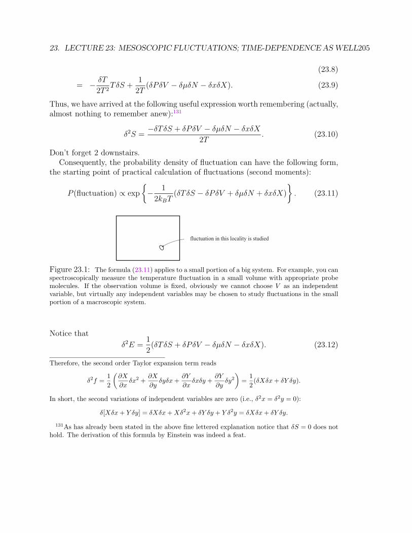
23. LECTURE 23: MESOSCOPIC FLUCTUATIONS; TIME-DEPENDENCE AS WELL205
(23.8)
= − δT
2T 2TδS +
1
2T(δPδV − δµδN − δxδX). (23.9)
Thus, we have arrived at the following useful expression worth remembering (actually,almost nothing to remember anew):131
δ2S =−δTδS + δPδV − δµδN − δxδX
2T. (23.10)
Don’t forget 2 downstairs.Consequently, the probability density of fluctuation can have the following form,
the starting point of practical calculation of fluctuations (second moments):
P (fluctuation) ∝ exp
− 1
2kBT(δTδS − δPδV + δµδN + δxδX)
. (23.11)
fluctuation in this locality is studied
Figure 23.1: The formula (23.11) applies to a small portion of a big system. For example, you canspectroscopically measure the temperature fluctuation in a small volume with appropriate probemolecules. If the observation volume is fixed, obviously we cannot choose V as an independentvariable, but virtually any independent variables may be chosen to study fluctuations in the smallportion of a macroscopic system.
Notice that
δ2E =1
2(δTδS + δPδV − δµδN − δxδX). (23.12)
Therefore, the second order Taylor expansion term reads
δ2f =12
(∂X
∂xδx2 +
∂X
∂yδyδx +
∂Y
∂xδxδy +
∂Y
∂yδy2
)=
12(δXδx + δY δy).
In short, the second variations of independent variables are zero (i.e., δ2x = δ2y = 0):
δ[Xδx + Y δy] = δXδx + Xδ2x + δY δy + Y δ2y = δXδx + δY δy.
131As has already been stated in the above fine lettered explanation notice that δS = 0 does nothold. The derivation of this formula by Einstein was indeed a feat.
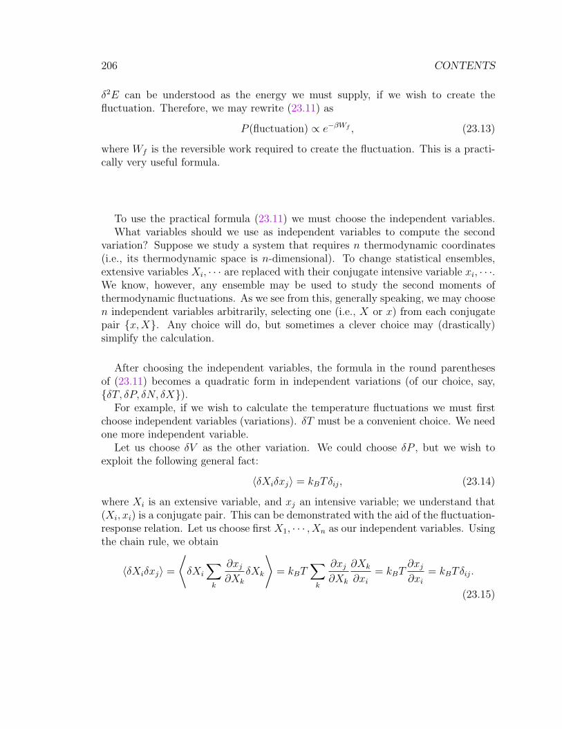
206 CONTENTS
δ2E can be understood as the energy we must supply, if we wish to create thefluctuation. Therefore, we may rewrite (23.11) as
P (fluctuation) ∝ e−βWf , (23.13)
where Wf is the reversible work required to create the fluctuation. This is a practi-cally very useful formula.
To use the practical formula (23.11) we must choose the independent variables.What variables should we use as independent variables to compute the second
variation? Suppose we study a system that requires n thermodynamic coordinates(i.e., its thermodynamic space is n-dimensional). To change statistical ensembles,extensive variables Xi, · · · are replaced with their conjugate intensive variable xi, · · ·.We know, however, any ensemble may be used to study the second moments ofthermodynamic fluctuations. As we see from this, generally speaking, we may choosen independent variables arbitrarily, selecting one (i.e., X or x) from each conjugatepair x,X. Any choice will do, but sometimes a clever choice may (drastically)simplify the calculation.
After choosing the independent variables, the formula in the round parenthesesof (23.11) becomes a quadratic form in independent variations (of our choice, say,δT, δP, δN, δX).
For example, if we wish to calculate the temperature fluctuations we must firstchoose independent variables (variations). δT must be a convenient choice. We needone more independent variable.
Let us choose δV as the other variation. We could choose δP , but we wish toexploit the following general fact:
〈δXiδxj〉 = kBTδij, (23.14)
where Xi is an extensive variable, and xj an intensive variable; we understand that(Xi, xi) is a conjugate pair. This can be demonstrated with the aid of the fluctuation-response relation. Let us choose first X1, · · · , Xn as our independent variables. Usingthe chain rule, we obtain
〈δXiδxj〉 =
⟨δXi
∑k
∂xj
∂Xk
δXk
⟩= kBT
∑k
∂xj
∂Xk
∂Xk
∂xi
= kBT∂xj
∂xi
= kBTδij.
(23.15)
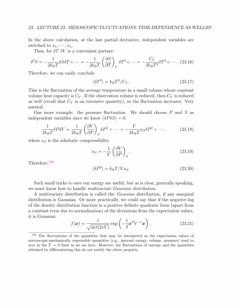
23. LECTURE 23: MESOSCOPIC FLUCTUATIONS; TIME-DEPENDENCE AS WELL207
In the above calculation, at the last partial derivative, independent variables areswitched to x1, · · · , xn.
Thus, for δT δV is a convenient partner:
δ2S = − 1
2kBTδSδT+· · · = − 1
2kBT
(∂S
∂T
)V
δT 2+· · · = − CV
2kBT 2δT 2+· · · . (23.16)
Therefore, we can easily conclude
〈δT 2〉 = kBT2/CV . (23.17)
This is the fluctuation of the average temperature in a small volume whose constantvolume heat capacity is CV . If the observation volume is reduced, then CV is reducedas well (recall that CV is an extensive quantity), so the fluctuation increases. Verynatural.
One more example: the pressure fluctuation. We should choose P and S asindependent variables since we know 〈δPδS〉 = 0:
1
2kBTδPδV =
1
2kBT
(∂V
∂P
)S
δP 2 + · · · = − V
2kBTκSδP
2 + · · · , (23.18)
where κS is the adiabatic compressibility
κS = − 1
V
(∂V
∂P
)S
. (23.19)
Therefore,132
〈δP 2〉 = kBT/V κS. (23.20)
Such small tricks to save our energy are useful, but as is clear, generally speaking,we must know how to handle multivariate Gaussian distribution.
A multivariate distribution is called the Gaussian distribution, if any marginaldistribution is Gaussian. Or more practically, we could say that if the negative logof the density distribution function is a positive definite quadratic form (apart froma constant term due to normalization) of the deviations from the expectation values,it is Gaussian:
f(x) =1√
det(2πV )exp
(−1
2xTV −1x
), (23.21)
132 The fluctuations of the quantities that may be interpreted as the expectation values ofmicroscopic-mechanically expressible quantities (e.g., internal energy, volume, pressure) tend tozero in the T → 0 limit as we see here. However, the fluctuations of entropy and the quantitiesobtained by differentiating this do not satisfy the above property.
208 CONTENTS
where V is the covariance matrix defined by (do not forget that our vectors arecolumn vectors)
V = 〈xxT 〉. (23.22)
If the mean value of x is nonzero 〈x〉 = m, simply replace x in the above with x−m.The reader must not have any difficulty in demonstrating that (23.21) is correctlynormalized. [Hint: choose eigendirections of V as the orthogonal coordinates.]
In particular, for the two variable case:
f(x, y) ∝ exp
−1
2
(ax2 + 2bxy + cy2
), (23.23)
then
V = Λ−1 =
(a bb c
)−1
=1
detΛ
(c −b−b a
)(23.24)
That is,
〈x2〉 = c/detΛ, 〈xy〉 = −b/detΛ, 〈y2〉 = a/detΛ. (23.25)
The following topic requires a couple of weeks, but here it is outlined as a ‘col-loquium’ before one week recess. After Thanksgiving, we still have 8 lectures, so Ihope we can cover interesting topics related to phase transitions, the real statisticalmechanics.
We wish to discuss nonequilibrium dissipative phenomena. However, we are notvery ambitious to study general nonequilibrium; we study small deviations that maybe governed by linear phenomenological laws.
If a macroscopic system is not in equilibrium but slightly away from equilibrium,the system may still be described in terms of thermodynamic variables. These vari-ables will be time-dependent. Since the deviation of entropy from its maximum valuedescribes the extent of nonequilibrium, entropy S suitably extended to the near-equilibrium states must determine the driving force for nonequilibrium processes.Thus, the phenomenological macroscopic laws have the following form:
dX
dt= L
∂S
∂X, (23.26)
23. LECTURE 23: MESOSCOPIC FLUCTUATIONS; TIME-DEPENDENCE AS WELL209
where L is called an Onsager coefficient. Here, we consider the simplest case de-scribed by a single extensive quantity X (without spatial inhomogeneity). For sim-plicity we assume X = 0 in equilibrium. S(X) is not the true equilibrium entropy;since we have only to study linear evolution laws, we need S(X) to order X2, andthe coefficient may be computed from the second derivative of S around equilibriumstates.133
Let us try to describe the nonequilibrium system on the mesoscopic scale. We canexpect a Langevin equation
dX
dT= L
∂S
∂X+ w. (23.27)
Since the time derivative in this equation is not truly microscopic time derivative,but the coarse-grained one, let us denote it as ∆/∆t: it is the true time derivatived/dt averaged over mesoscopically small time ∆t. We assume the large deviationframework of the following form:
P
(∆X
∆t∼ X
)≈ exp[−∆tI(X)], (23.28)
where the rate function I is zero if
X = L∂S
∂X, (23.29)
the phenomenological law. This means that the most probable time evolution isaccording to the linear phenomenology. This assertion is called Onsager’s princi-ple (interpreted in a modern fashion proposed by the lecturer long ago). Onsagerassumed a simple quadratic form for the rate function:
I(X) =1
4Γ
(X − L ∂S
∂X
)2
, (23.30)
where Γ is a positive constant describing the magnitude of the fluctuation. That is,the noise w is governed by the following Gaussian distribution:
P (w) ∝ e−∆tΓw2/4. (23.31)
133The reader may say that we should use a more appropriate thermodynamic potential insteadof S, but as explained before, since we need only the quadratic order results for the potential, weneed not worry about this question.
210 CONTENTS
Therefore, this Gaussian approximation for I is quite reasonable.
The numerical factor Γ may be related to the variance of X. Let us compute it.Obviously,
2
Γ= ∆t
(〈X2〉 − 〈X〉2
). (23.32)
Here, 〈 〉 implies the ensemble average (you repeat experiments!). Notice that Xconsists of two parts, the systematic part L∂S/∂X and the noise w. Note that∆t〈X2〉 = O[1], and 〈X〉 = O[1], so the first term on the RHS of (23.32) is muchlarger than the second term (because of noise squared):
1
Γ=
1
2∆t〈X2〉 =
1
2∆t
∫ ∆t
0
ds
∫ ∆t
0
ds′⟨dX
dt(s)
dX
dt(s′)
⟩. (23.33)
This double integration may be decomposed as∫ ∆t
0
ds
∫ ∆t
0
ds′ =
∫ ∆t
0
ds
∫ s
0
ds′ +
∫ ∆t
0
ds′∫ s
0
ds = 2
∫ ∆t
0
ds
∫ s
0
ds′, (23.34)
so1
Γ=
1
∆t
∫ ∆t
0
ds
∫ s
0
ds′⟨dX
dt(s)
dX
dt(s′)
⟩. (23.35)
Within the range of ∆t (very short from our point of view), the system may beassumed to be stationary (i.e., from the microscopic point of view ∆t is large andthis time span is rather uniform), so
1
Γ=
1
∆t
∫ ∆t
0
ds
∫ s
0
ds′⟨dX
dt(s− s′)dX
dt(0)
⟩=
1
∆t
∫ ∆t
0
ds
∫ s
0
dτ
⟨dX
dt(τ)
dX
dt(0)
⟩.
(23.36)We know the noise is uncorrelated, so the upper bound of the integral for τ does notdepend on s (even if it is replaced by ∞ the result does not change). Hence,
1
Γ=
∫ ∞
0
dτ
⟨dX
dt(τ)
dX
dt(0)
⟩. (23.37)
We know, from our experience with the Brownian motion, that Γ cannot be chosenfreely for the system. The noise amplitude and the dissipation rate L are related(fluctuation-dissipation relation we learned long ago):
L =1
kBΓ. (23.38)
23. LECTURE 23: MESOSCOPIC FLUCTUATIONS; TIME-DEPENDENCE AS WELL211
This implies that the kinetic coefficient L can be described in terms of the correlationfunction:
L =1
kB
∫ ∞
0
dt
⟨dX
dt(t)dX
dt(0)
⟩. (23.39)
This is called the Green-Kubo relation. Basically, the transport coefficient L is de-scribed in terms of a time correlation function of the ‘changes.’
Let us summarize what we have learned, while generalizing the formulas to themany variable case.
The phenomenological law is (corresponding to (23.29))
Xi =∑
j
Lij∂S
∂Xj
, (23.40)
where Lij are Onsager coefficients. The rate function for Xi is (corresponding to(23.30))
I(Xi(t)|Xi(t)) =1
4
∑ij
Γij
(Xi(t)−
∑i′
Lii′∂S(t)
∂Xi′(t)
)(Xj(t)−
∑j′
Ljj′∂S(t)
∂Xj′(t)
),
(23.41)where
kBΓij = (L−1)ij (23.42)
is the fluctuation-dissipation relation with an explicit form corresponding to (23.39):
Lij =1
kB
∫ ∞
0
ds
⟨dXi
dt(s)
dXj
dt(0)
⟩. (23.43)
The Langevin equation is (corresponding to (23.27))
Xi =∑
j
Lij∂S
∂Xj
+ wi (23.44)
with the noise satisfying 〈wi〉 = 0 and
〈wi(t)wj(s)〉 = 2LijkBδ(t− s). (23.45)
The average appearing in the formula for Lij is computed in the equilibrium state,so it does not depend on the absolute time. Therefore,⟨
dXi
dt(s)
dXj
dt(0)
⟩=
⟨dXi
dt(0)
dXj
dt(−s)
⟩=
⟨dXj
dt(−s)dXi
dt(0)
⟩. (23.46)
212 CONTENTS
Microscopic mechanics is time-reversal symmetric, so this implies⟨dXi
dt(s)
dXj
dt(0)
⟩= =
⟨dXj
dt(s)
dXi
dt(0)
⟩. (23.47)
Hence, we concludeLij = Lji. (23.48)
This is called Onsager’s reciprocity relation.
Appendix: Green-Kubo formula for transport coefficientsWe have given a general expression for the Onsager coefficients L in (23.43), but for spatially uniformsystems. The general nonequilibrium states are spatially nonuniform, so we need phenomenologyfor densities xi of extensive quantities Xi.
Probably, the easiest approach is to divide the space into cells and the variables in each cell xare denoted with the representative cell position as x(r). Then, we interpret (23.40) as (we write∂S/∂x = F )
∂x(r)∂t
=∑r′
L(r, r′)F (r′). (23.49)
Extending (23.43), let us first proceed quite formally without paying attention to the convergenceof the time integral:∑
r′
L(r, r′)F (r′) =1
kB
∫ ∞
0
dt∑r′
⟨∂x(r, t)
∂t
∂x(r′)T
∂t
⟩F (r′), (23.50)
=1
kB
∫ ∞
0
dt∑r′
〈div j(r, t) div j(r′)T 〉F (r′), (23.51)
= −divr
∫ ∞
0
dt∑r′
〈j(r, t)j(r′)T 〉∇r′F (r′) (23.52)
Here, j is the fluctuating part of the flux (non-systematic part): here we discuss the phenomenologyof the following form
∂x(r)∂t
= −divj(r) + σ, (23.53)
where σ is a source term we do not discuss, and j is the flux of x. Heat conduction, hydrodynamics,electric conduction, etc., are all in this form. The linear phenomenological law assumes the followingform for the flux (we discussed this when we learned viscosity):
j = L∇F. (23.54)
If F changes slowly compared with the correlation length of fluctuating flux, we may set r′ = r inF , and we arrive at
L =1
kB
∫ ∞
0
dt
∫dr⟨j(r, t)j(0)T
⟩. (23.55)
If we introduceJ(t) =
∫dr j(r, t), (23.56)
23. LECTURE 23: MESOSCOPIC FLUCTUATIONS; TIME-DEPENDENCE AS WELL213
thenL =
1V kB
∫ ∞
0
dt⟨J(t)J(0)T
⟩. (23.57)
Here, V is the volume of the system (or the domain being paid attention). This is almost the finalresult.
However, the time integral in (23.57) may not exist, because limt→∞ J may not be zero. Toavoid this, we can simply subtract this value from J , and define J− = J − limt→∞ J to obtain thefinal result:
L =1
V kB
∫ ∞
0
dt 〈J−(t)J−(0)T 〉. (23.58)
This is the Green-Kubo formula for transport coefficients.
214 CONTENTS
24 Lecture 24: Phases and phase transitions
Summary∗ Qualitative change of phases is the phase transition, which corresponds to somesingularities of thermodynamic potentials.∗ Phase coexistence conditions (under given T and P ) are a set of equalities amongchemical potentials. Gibbs’ phase rule follows from the condition.∗ Thermodynamic limit is absolutely needed to rationalize phase transitions statistical-mechanically.
Key wordsphase, phase transition, phase diagram, coexistence curve, triple point, kelvin scale,Clausius-Clapeyron equation, Gibbs’ phase rule, first order phase transition, higherorder phase transition, Ising model, thermodynamic limit.
What you should be able to do∗ You must be able to draw the phase diagram of a ordinary one-component fluidon the PT plane.∗ You must be able to sketch G(T, P ) for an ordinary fluid.
So far we have not discussed systems with interactions. If there are interactions,there are various phases as is exemplified by ice, liquid and vapor of water. First,let us discuss how to describe what we experience thermodynamically. Then, let usdiscuss whether statistical mechanics can discuss phase transitions.
What is a phase?Intuitively, under different conditions (say, at various (T, P )) a system can exhibit
qualitatively different properties; we say the system is in different phases.134 To un-derstand a substance is to understand its various phases. Therefore, we wish to mapout what happens at various points in the thermodynamic space or at least in termsof thermodynamic parameters (e.g., T , P , etc.), i.e., we wish to construct the phasediagram (see, e.g., Fig. 24.1). To understand the world map we must understandwhere the state boundaries are and what the features of the territories are. To un-
134We may say an equilibrium state is in a single phase, if it is macroscopically homogeneous.
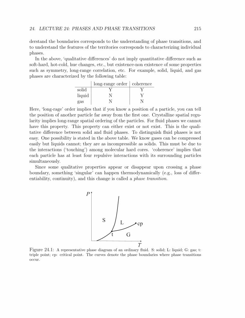
24. LECTURE 24: PHASES AND PHASE TRANSITIONS 215
derstand the boundaries corresponds to the understanding of phase transitions, andto understand the features of the territories corresponds to characterizing individualphases.
In the above, ‘qualitative differences’ do not imply quantitative difference such assoft-hard, hot-cold, hue changes, etc., but existence-non existence of some propertiessuch as symmetry, long-range correlation, etc. For example, solid, liquid, and gasphases are characterized by the following table:
long-range order coherencesolid Y Yliquid N Ygas N N
Here, ‘long-rage’ order implies that if you know a position of a particle, you can tellthe position of another particle far away from the first one. Crystalline spatial regu-larity implies long-range spatial ordering of the particles. For fluid phases we cannothave this property. This property can either exist or not exist. This is the quali-tative difference between solid and fluid phases. To distinguish fluid phases is noteasy. One possibility is stated in the above table. We know gases can be compressedeasily but liquids cannot; they are as incompressible as solids. This must be due tothe interactions (‘touching’) among molecular hard cores. ‘coherence’ implies thateach particle has at least four repulsive interactions with its surrounding particlessimultaneously.
Since some qualitative properties appear or disappear upon crossing a phaseboundary, something ‘singular’ can happen thermodynamically (e.g., loss of differ-entiability, continuity), and this change is called a phase transition.
T
P
LS
Gt
cp
Figure 24.1: A representative phase diagram of an ordinary fluid. S: solid; L: liquid; G: gas; t:triple point; cp: critical point. The curves denote the phase boundaries where phase transitionsoccur.
216 CONTENTS
However, a precise definition of ‘phase’ is actually rather difficult. Near the phaseboundaries we may clearly distinguish the phases, but the ‘territory where a phaseoccupies’ may not be well-defined as in the case of gases and liquids. Therefore,here, the concept of ‘phase’ is used ‘locally’ when precise statements are needed. Wesay the states (near the phase transition point) that cannot be changed into eachother without a phase transition (= thermodynamic singularity) are distinct (nearthe phase transition).
First, let us summarize thermodynamic aspects of phases and phase transitions.If there is a phase transition from one phase to another, there may or may not be acoexistence of these phases. Let us assume the phase coexistence is possible (as inthe case of ice and liquid water) and discuss what is required for phases to coexistand what the requirements entail.135
Suppose a system is described by its thermodynamic coordinates (E,X) and twophases I and II coexist in equilibrium while E and X exchange being allowed betweenthe phases (in an isolated box). We know S = SI + SII must be maximized, so theequilibrium condition is the identity of T and x/T as we discussed long ago. Let usreview it. The Gibbs relation implies
δS =1
TδE − x
TδX. (24.1)
Here, δ implies variation or virtual change, BUT in reality fluctuations actuallyrealize these needed changes spontaneously. δEI + δEII = 0 and dXI + δXII = 0imply the following equilibrium condition:
δS =1
TIδEI−
xITIδXI +
1
TIIδEII−
xIITII
δXII =
(1
TI− 1
TII
)δEI−
(xITI− xIITII
)δXI = 0
(24.2)Therefore, TI = TII and xI = xII are required in general. Usually, X = V and N , soT, P and µ must be identical between two phases:
TI = TII, PI = PII, µI = µII. (24.3)
The last equality in (24.3) is
µI(T, P ) = µII(T, P ). (24.4)
135However, it is impossible to know whether the given two phases coexist or not purely thermo-dynamically, although, usually, we may say the phases satisfying the thermodynamic coexistenceconditions do coexist.
24. LECTURE 24: PHASES AND PHASE TRANSITIONS 217
This functional relation determines a curve called the coexistence curve in the T -Pdiagram (see Fig. 24.1).136
Along this line the Gibbs free energy G of the whole system may be writtenas
G = NIµI +NIIµII. (24.5)
Thus, without changing the value ofG, any mass ratio of the two phases is admissible.This implies that in the phase diagram described in the thermodynamic space phasecoexistence is described as a boundary ‘mine field’ instead of a line.
How many phases can coexist at a given T and P? Suppose we have X coexistingphases. The following conditions must be satisfied:
µI(T, P ) = µII(T, P ) = · · · = µX(T, P ). (24.6)
We believe that for the generic case, µ’s are sufficiently functionally independent. Tobe able to solve for T and P , we can allow at most two independent relations. Thatis, at most three phases can coexist at a given T and P for a pure substance.
For a pure substance, if three phases coexist, T and P are uniquely fixed. Thispoint on the T -P diagram is called the triple point. The kelvin scale of temperatureis defined so that triple point of water is at T = 273.16K (since 1954). t = T −273.15is the temperature in Celsius. Again, this is the definition of C.
How can we draw the coexistence curve? For a pure substance, as we have seen,the chemical potentials of coexisting phases must be identical. Before and after thephase transition from phase I to II or vice versa, there is no change of the Gibbs freeenergy
∆GCC = 0, (24.7)
where CC means “along the coexistence curve” and ∆ implies the difference acrossthe coexistence curve (say, phase I − phase II). This should be true even if we changeT and P simultaneously along the coexistence curve. Hence, along CC (i.e., (T, P )and (T + dT, P + dP ) are both on the coexistence curve)
−∆SdT + ∆V dP = 0⇒(∂P
∂T
)CC
=∆S
∆V. (24.8)
136(24.4) may be obtained by minimizing the Gibbs free energy under constant T and P , becausein the thermodynamic limit (i.e., if the system is large enough) what we can obtain from anisolated system and the same system under T, P constant condition with the consistent T and Pare indistinguishable (ensemble equivalence).
218 CONTENTS
At the phase transition ∆H = T∆S, where ∆H is the latent heat and T the phasetransition temperature. Thus, we can rewrite (24.8) as(
∂P
∂T
)CC
=∆I→IIH
T∆I→IIV, (24.9)
where ∆I→IIX denotes XII −XI. This relation is called the Clapeyron-Clausius re-lation.
Consider a more general case of a system consisting of c chemically independentcomponents (i.e., the number of components we can change independently). Forexample, H3O
+ in pure water should not be counted, if we count H2O among theindependent chemical components.
Suppose there are φ coexisting phases. The equilibrium conditions are:(1) T and P must be common to all the phases,(2) The chemical potentials of the c chemical species must be common to all thephases.
To specify the composition of a phase we need c − 1 variables, because we needonly the concentration ratio. Thus, the chemical potential for a chemical speciesdepends on T , P and c−1 mole fractions (x1, x2, · · · , xc−1), which are not necessarilycommon to all the phases (we must add a suffix to denote the phases). That is, µ’sare c + 1 variable functions, and we have 2 + φ(c− 1) unknown variables. We haveφ− 1 equalities among the chemical potentials in different phases for each chemicalspecies, so the number of equalities we have is (φ − 1) × c. Look at the followingsimultaneous equations:
µ1I(T, P, x
1I , x
2I , · · ·x
c−1I ) = µ1
II(T, P, x1II, x
2II, · · ·x
c−1II ) = · · · = µ1
φ(T, P, x1φ, x
2φ, · · ·xc−1
φ ),
· · ·µj
I(T, P, x1I , x
2I , · · ·x
c−1I ) = µj
II(T, P, x1II, x
2II, · · ·x
c−1II ) = · · · = µj
φ(T, P, x1φ, x
2φ, · · ·xc−1
φ ),
· · ·µc
I(T, P, x1I , x
2I , · · ·x
c−1I ) = µc
II(T, P, x1II, x
2II, · · ·x
c−1II ) = · · · = µc
φ(T, P, x1φ, x
2φ, · · ·xc−1
φ ),
(24.10)
Consequently, for the generic case we can choose f = 2+φ(c−1)−c(φ−1) = c+2−φvariables freely. This number f is called the number of thermodynamic degrees offreedom. We have arrived at the Gibbs phase rule:137
f = c+ 2− φ. (24.11)
137As astute readers have probably sensed already, the derivation is not water tight. Rigorously
24. LECTURE 24: PHASES AND PHASE TRANSITIONS 219
What happens to the Gibbs free energy at the phase transition point under con-stant T and P ? You must be able to sketch it in the ordinary fluid case. Note theusual Gibbs relation:
dG = −SdT + V dP. (24.12)
Under constant P , G may be sketched as follows:
T
G
SL
G
melting
point
boiling
point
Figure 24.2: Typical behavior of Gibbs free energy for a pure substance. The free energy losesdifferentiability at first order phase transition points.
When P is the critical pressure, then the liquid-gas transition ‘break’ disappears:G becomes differentiable. However, the specific heat has a singular behavior at thecritical temperature. That is, the LG transition becomes second order.
Try to sketch G nder constant T as a function of P .
Usually, phase transitions are classified into first order phase transitions and therest called continuous phase transitions or second-order phase transitions. In the firstorder phase transition at least one thermodynamic density (= extensive quantity pervolume) changes discontinuously, but in the second order phase transitions there isno discontinuity in thermodynamic densities. The liquid-gas transition at the criticalpressure is a second-order phase transition as noted just above.
You might think that first order phase transitions are much more drastic and typi-cal phase transitions, but actually as we will see later, it is not. Phase transitions arealways between more ordered and less ordered phases; it is between the low entropystate and the high energy (enthalpy) state. For example melting is the transitionfrom low entropy solid to high energy liquid. Protein folding is the transition fromhigher energy random coil state to low entropy folded state.138
speaking, we cannot derive the phase rule from the fundamental laws of thermodynamics (norequilibrium statistical mechanics, either).
138However, do not have a prejudice that natural states of proteins are equilibrium states. Manylarge proteins are likely to be in metastable states when they function biologically normally.
220 CONTENTS
A first order phase transition occurs when the ordered phase loses its stability‘prematurely.’ In other words the first order phase transition occurs when the orderbecomes fragile against small thermal fluctuations. In contrast, in the case of secondorder phase transitions the ordered phase persists until it completely loses its order.Thus, the second order phase transition is theoretically the most interesting. There-fore, we discuss the second order phase transition first.
A typical second order phase transition is the one from the paramagnetic to theferromagnetic phase.
A magnet can be understood as a lattice of spins interacting with each otherlocally in space. The interaction between two spins has a tendency to align themparallelly. At higher temperatures, due to vigorous thermal motions, this interactioncannot quite make order among spins, but at lower temperatures the entropic effectbecomes less significant, so spins order globally. There is a special temperature Tc
below which this ordering occurs. We say an order-disorder transition occurs at thistemperature.
The Ising model is the simplest model of this transition. At each lattice point isa (classical) spin σ which takes only +1 (up) or −1 (down). A nearest neighbor spinpair has the following interaction energy:
− Jσiσj, (24.13)
where J is called the coupling constant, which is positive in our example (ferromag-netic case). We assume all the spin-spin interaction energies are superposable, so thetotal energy of the system for a lattice is given by
H = −∑〈i,j〉
Jσiσj −∑
i
hσi, (24.14)
where 〈 〉 implies the nearest neighbor pairs, and h is the external magnetic field.The (generalized canonical) partition function for this system reads
Z =∑
σi=±1
e−βH. (24.15)
Here, the sum is over all spin configurations.139
139What is −kBT log Z in this case? It is NOT the Helmholtz free energy in the original sense.
24. LECTURE 24: PHASES AND PHASE TRANSITIONS 221
So far phenomenologically, we accepted the existence of phase transitions, and dis-cussed how to describe/handle them. From the statistical mechanics point of view,the most important question is why such qualitative changes can occur at all. Actu-ally, a more fundamental question is: can statistical mechanics ever describe phasetransitions? Up to early 1930s such doubts existed. Now, in the 21st century, we aresure that statistical mechanics correctly describes various phase transitions. HOW-EVER, do not forget that we cannot yet explain why ordinary molecules can makecrystals statistical mechanically below some finite temperature. Does the partitionfunction contain a crystal? We believe so, but no one has demonstrated this.
If the system size is finite, the sum in (24.15) is a finite sum of positive terms.Each term in this sum is analytic in T and h, so the sum itself becomes analytic inT and h (i.e., very smooth). Furthermore, Z cannot be zero, because each term inthe sum is strictly positive. Therefore, its logarithm is analytic in T and h; the freeenergy of the finite lattice system cannot exhibit any singularity. That is, there is nothermodynamic singularity, and consequently, there is no phase transition for thissystem.140
Even in the actual system we study experimentally, there are only a finite numberof atoms, but this number is huge. Thus, the question of phase transitions from thestatistical mechanics point of view is: is there any singularity in A = −kBT logZ inthe large system limit? The large system limit, with proper caution not to increaseits surface area more than the order of V 2/3, where V is the system volume, is calledthe thermodynamic limit. Strictly speaking, phase transitions can occur only in thislimit.
Notice that qualitative changes require loss of analyticity.
We started to discuss Peierls’ argument: Peierls proved that Z contains a ferro-magnetic phase transition in the thermodynamic limit. Let us continue this the dayafter tomorrow.
140Strictly speaking, there is no phase transition for any finite system, unless each spin hasinfinitely many states.
222 CONTENTS
25 Lecture 25: Spatial dimensionality and inter-
action range are crucial
Summary∗ Statistical mechanics seems to be able to explain various phases and phase transi-tions rationally in the thermodynamic limit.∗ Spatial dimensionality is crucial to the phase ordering and existence of the order-disorder phase transition. Peierls’ argument can often tell whether a system canorder when sufficiently cooled.∗ If the interaction is long-ranged, phase transitions can happen even in 1-space.(Augmented) van der Waals gas in 1D is a typical example.∗ The second order phase transition for magnets, fluids and binary fluid mixturesmay be understood in a unified fashion.
Key wordsPeierls’ argument, Kac potential, van der Waals gas, Maxwell’s rule, Tonks’ gas,
What you should be able to do∗ Intuitively understand why spatial dimensionality matters.∗ You must be able to explain Peierls’ argument.∗ Derivation of Tonk’s equation of state should be a good exercise.
Whether statistical mechanics can understand phase transitions or not in thethermodynamic limit is a fundamental question. Peierls definitely settled the issueby demonstrating that the 2D Ising model has an ordered phase. His demonstrationmakes it clear that spatial dimensionality is crucial.
The Ising model due to Lenz was introduced in the preceding lecture, whoseHamiltonian reads
H = −J∑〈i,j〉
σiσj − h∑
i
σi. (25.1)
We can interpret this as a lattice model of a gas (lattice gas) with the followingcorrespondence ‘down’ (‘up’) → lattice point ‘occupied’ (‘empty’). h may be inter-preted as the chemical potential (large positive h implies more down spins = more
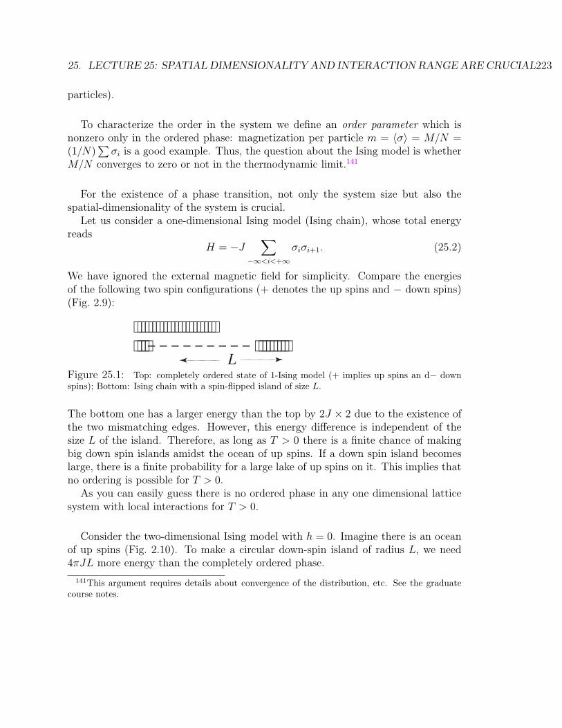
25. LECTURE 25: SPATIAL DIMENSIONALITY AND INTERACTION RANGE ARE CRUCIAL223
particles).
To characterize the order in the system we define an order parameter which isnonzero only in the ordered phase: magnetization per particle m = 〈σ〉 = M/N =(1/N)
∑σi is a good example. Thus, the question about the Ising model is whether
M/N converges to zero or not in the thermodynamic limit.141
For the existence of a phase transition, not only the system size but also thespatial-dimensionality of the system is crucial.
Let us consider a one-dimensional Ising model (Ising chain), whose total energyreads
H = −J∑
−∞<i<+∞
σiσi+1. (25.2)
We have ignored the external magnetic field for simplicity. Compare the energiesof the following two spin configurations (+ denotes the up spins and − down spins)(Fig. 2.9):
+ + + + + + + + + + + + + + + + + + + + + + + + + + − − − − − − − − − + + + + + + + + +
L
Figure 25.1: Top: completely ordered state of 1-Ising model (+ implies up spins an d− downspins); Bottom: Ising chain with a spin-flipped island of size L.
The bottom one has a larger energy than the top by 2J × 2 due to the existence ofthe two mismatching edges. However, this energy difference is independent of thesize L of the island. Therefore, as long as T > 0 there is a finite chance of makingbig down spin islands amidst the ocean of up spins. If a down spin island becomeslarge, there is a finite probability for a large lake of up spins on it. This implies thatno ordering is possible for T > 0.
As you can easily guess there is no ordered phase in any one dimensional latticesystem with local interactions for T > 0.
Consider the two-dimensional Ising model with h = 0. Imagine there is an oceanof up spins (Fig. 2.10). To make a circular down-spin island of radius L, we need4πJL more energy than the completely ordered phase.
141This argument requires details about convergence of the distribution, etc. See the graduatecourse notes.
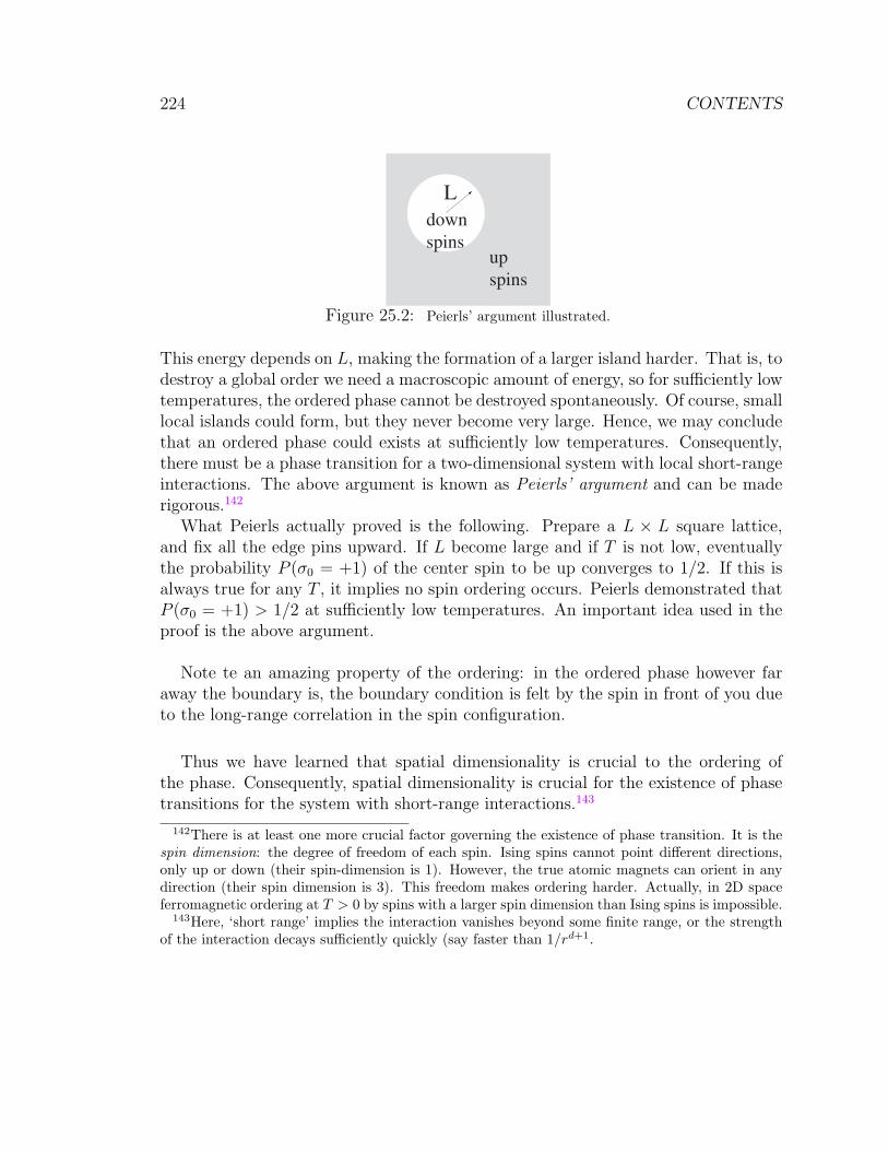
224 CONTENTS
L
up
spins
down
spins
Figure 25.2: Peierls’ argument illustrated.
This energy depends on L, making the formation of a larger island harder. That is, todestroy a global order we need a macroscopic amount of energy, so for sufficiently lowtemperatures, the ordered phase cannot be destroyed spontaneously. Of course, smalllocal islands could form, but they never become very large. Hence, we may concludethat an ordered phase could exists at sufficiently low temperatures. Consequently,there must be a phase transition for a two-dimensional system with local short-rangeinteractions. The above argument is known as Peierls’ argument and can be maderigorous.142
What Peierls actually proved is the following. Prepare a L × L square lattice,and fix all the edge pins upward. If L become large and if T is not low, eventuallythe probability P (σ0 = +1) of the center spin to be up converges to 1/2. If this isalways true for any T , it implies no spin ordering occurs. Peierls demonstrated thatP (σ0 = +1) > 1/2 at sufficiently low temperatures. An important idea used in theproof is the above argument.
Note te an amazing property of the ordering: in the ordered phase however faraway the boundary is, the boundary condition is felt by the spin in front of you dueto the long-range correlation in the spin configuration.
Thus we have learned that spatial dimensionality is crucial to the ordering ofthe phase. Consequently, spatial dimensionality is crucial for the existence of phasetransitions for the system with short-range interactions.143
142There is at least one more crucial factor governing the existence of phase transition. It is thespin dimension: the degree of freedom of each spin. Ising spins cannot point different directions,only up or down (their spin-dimension is 1). However, the true atomic magnets can orient in anydirection (their spin dimension is 3). This freedom makes ordering harder. Actually, in 2D spaceferromagnetic ordering at T > 0 by spins with a larger spin dimension than Ising spins is impossible.
143Here, ‘short range’ implies the interaction vanishes beyond some finite range, or the strengthof the interaction decays sufficiently quickly (say faster than 1/rd+1.
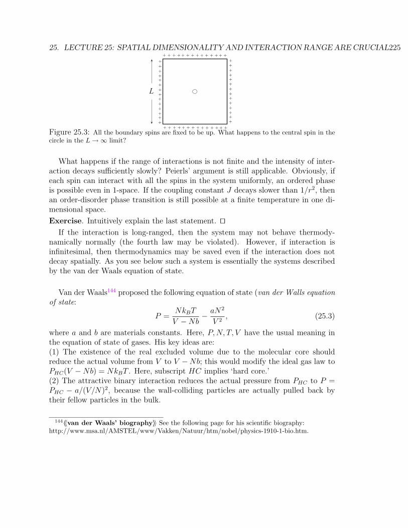
25. LECTURE 25: SPATIAL DIMENSIONALITY AND INTERACTION RANGE ARE CRUCIAL225
+
+
+
++
+
+
+
+
+
+
++
+
+
+
+
++
+
+
+
+
+
+
++
+
+ + + + + + + + + + + + + +
+ + + + + + + + + + + + + +
L
Figure 25.3: All the boundary spins are fixed to be up. What happens to the central spin in thecircle in the L→∞ limit?
What happens if the range of interactions is not finite and the intensity of inter-action decays sufficiently slowly? Peierls’ argument is still applicable. Obviously, ifeach spin can interact with all the spins in the system uniformly, an ordered phaseis possible even in 1-space. If the coupling constant J decays slower than 1/r2, thenan order-disorder phase transition is still possible at a finite temperature in one di-mensional space.
Exercise. Intuitively explain the last statement. utIf the interaction is long-ranged, then the system may not behave thermody-
namically normally (the fourth law may be violated). However, if interaction isinfinitesimal, then thermodynamics may be saved even if the interaction does notdecay spatially. As you see below such a system is essentially the systems describedby the van der Waals equation of state.
Van der Waals144 proposed the following equation of state (van der Walls equationof state:
P =NkBT
V −Nb− aN2
V 2, (25.3)
where a and b are materials constants. Here, P,N, T, V have the usual meaning inthe equation of state of gases. His key ideas are:(1) The existence of the real excluded volume due to the molecular core shouldreduce the actual volume from V to V −Nb; this would modify the ideal gas law toPHC(V −Nb) = NkBT . Here, subscript HC implies ‘hard core.’(2) The attractive binary interaction reduces the actual pressure from PHC to P =PHC − a/(V/N)2, because the wall-colliding particles are actually pulled back bytheir fellow particles in the bulk.
144〈〈van der Waals’ biography〉〉 See the following page for his scientific biography:http://www.msa.nl/AMSTEL/www/Vakken/Natuur/htm/nobel/physics-1910-1-bio.htm.
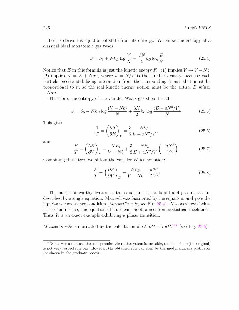
226 CONTENTS
Let us derive his equation of state from its entropy. We know the entropy of aclassical ideal monatomic gas reads
S = S0 +NkB logV
N+
3N
2kB log
E
N(25.4)
Notice that E in this formula is just the kinetic energy K. (1) implies V → V −Nb,(2) implies K = E + Nan, where n = N/V is the number density, because eachparticle receive stabilizing interaction from the surrounding ‘mass’ that must beproportional to n, so the real kinetic energy potion must be the actual E minus−Nan.
Therefore, the entropy of the van der Waals gas should read
S = S0 +NkB log(V −Nb)
N+
3N
2kB log
(E + aN2/V )
N. (25.5)
This gives1
T=
(∂S
∂E
)V
=3
2
NkB
E + aN2/V, (25.6)
andP
T=
(∂S
∂V
)E
=NkB
V −Nb+
3
2
NkB
E + aN2/V
(−aN
2
V 2
). (25.7)
Combining these two, we obtain the van der Waals equation:
P
T=
(∂S
∂V
)E
=NkB
V −Nb− aN2
TV 2. (25.8)
The most noteworthy feature of the equation is that liquid and gas phases aredescribed by a single equation. Maxwell was fascinated by the equation, and gave theliquid-gas coexistence condition (Maxwell’s rule, see Fig. 25.4). Also as shown belowin a certain sense, the equation of state can be obtained from statistical mechanics.Thus, it is an exact example exhibiting a phase transition.
Maxwell’s rule is motivated by the calculation of G: dG = V dP .145 (see Fig. 25.5)
145Since we cannot use thermodynamics where the system is unstable, the demo here (the original)is not very respectable one. However, the obtained rule can even be thermodynamically justifiable(as shown in the graduate notes).
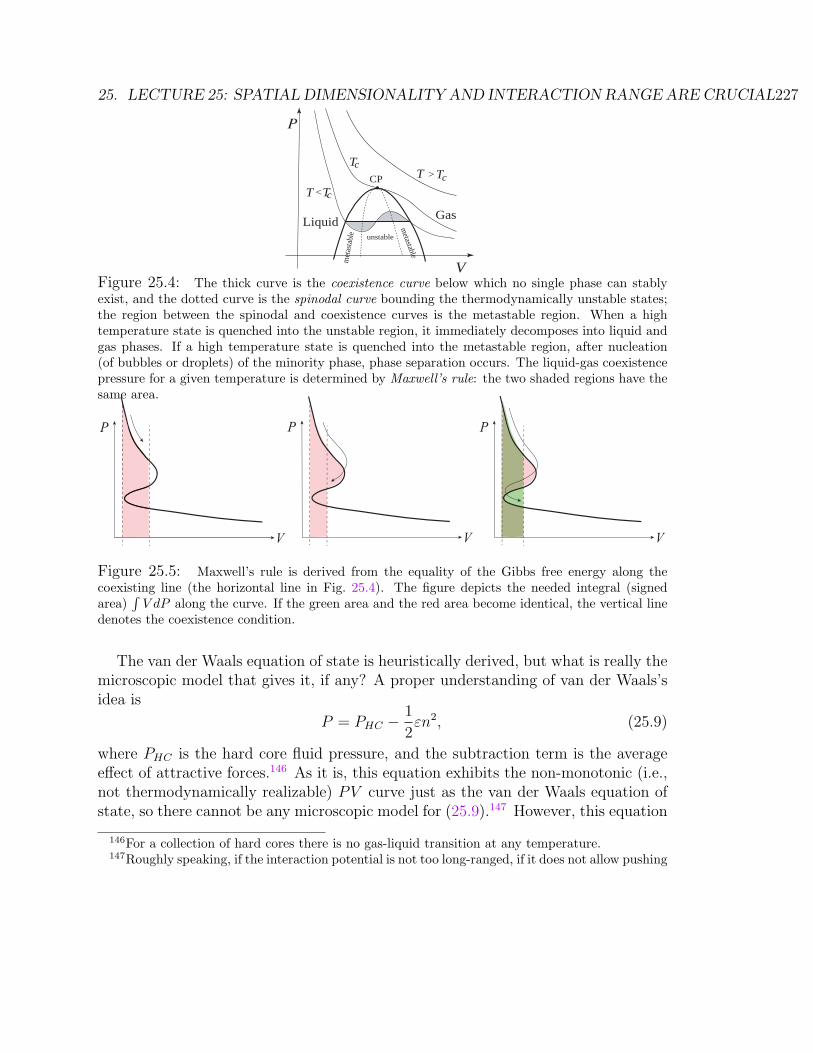
25. LECTURE 25: SPATIAL DIMENSIONALITY AND INTERACTION RANGE ARE CRUCIAL227
TT
Tc
c
c
T
T>
<CP
met
asta
ble
metastable
unstable
GasLiquid
V
P
Figure 25.4: The thick curve is the coexistence curve below which no single phase can stablyexist, and the dotted curve is the spinodal curve bounding the thermodynamically unstable states;the region between the spinodal and coexistence curves is the metastable region. When a hightemperature state is quenched into the unstable region, it immediately decomposes into liquid andgas phases. If a high temperature state is quenched into the metastable region, after nucleation(of bubbles or droplets) of the minority phase, phase separation occurs. The liquid-gas coexistencepressure for a given temperature is determined by Maxwell’s rule: the two shaded regions have thesame area.
P
V
P
V
P
V
Figure 25.5: Maxwell’s rule is derived from the equality of the Gibbs free energy along thecoexisting line (the horizontal line in Fig. 25.4). The figure depicts the needed integral (signedarea)
∫V dP along the curve. If the green area and the red area become identical, the vertical line
denotes the coexistence condition.
The van der Waals equation of state is heuristically derived, but what is really themicroscopic model that gives it, if any? A proper understanding of van der Waals’sidea is
P = PHC −1
2εn2, (25.9)
where PHC is the hard core fluid pressure, and the subtraction term is the averageeffect of attractive forces.146 As it is, this equation exhibits the non-monotonic (i.e.,not thermodynamically realizable) PV curve just as the van der Waals equation ofstate, so there cannot be any microscopic model for (25.9).147 However, this equation
146For a collection of hard cores there is no gas-liquid transition at any temperature.147Roughly speaking, if the interaction potential is not too long-ranged, if it does not allow pushing
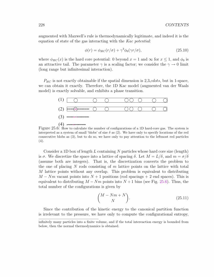
228 CONTENTS
augmented with Maxwell’s rule is thermodynamically legitimate, and indeed it is theequation of state of the gas interacting with the Kac potential:
φ(r) = φHC(r/σ) + γ3φ0(γr/σ), (25.10)
where φHC(x) is the hard core potential: 0 beyond x = 1 and∞ for x ≤ 1, and φ0 isan attractive tail. The parameter γ is a scaling factor; we consider the γ → 0 limit(long range but infinitesimal interaction).
PHC is not exactly obtainable if the spatial dimension is 2,3,cdots, but in 1-space,we can obtain it exactly. Therefore, the 1D Kac model (augmented van der Waalsmodel) is exactly solvable, and exhibits a phase transition.
(1)
(2)
(3)
(4)Figure 25.6: How to calculate the number of configurations of a 1D hard-core gas. The system isinterpreted as a system of small ‘blobs’ of size δ as (2). We have only to specify locations of the redconsecutive blobs as (3), but to do so, we have only to pay attention to the leftmost red particles(4).
Consider a 1D box of length L containing N particles whose hard core size (length)is σ. We discretize the space into a lattice of spacing δ. Let M = L/δ, and m = σ/δ(assume both are integers). That is, the discretization converts the problem tothe one of placing N rods consisting of m lattice points on the lattice with totalM lattice points without any overlap. This problem is equivalent to distributingM −Nm vacant points into N + 1 positions (rod spacings + 2 end spaces). This isequivalent to distributing M −Nm points into N + 1 bins (see Fig. 25.6). Thus, thetotal number of the configurations is given by(
M −Nm+N
N
). (25.11)
Since the contribution of the kinetic energy to the canonical partition functionis irrelevant to the pressure, we have only to compute the configurational entropy,
infinitely many particles into a finite volume, and if the total intereaction energy is bounded frombelow, then the normal thermodynamics is obtained.
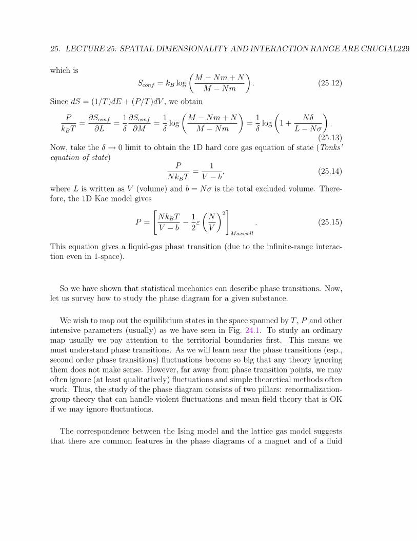
25. LECTURE 25: SPATIAL DIMENSIONALITY AND INTERACTION RANGE ARE CRUCIAL229
which is
Sconf = kB log
(M −Nm+N
M −Nm
). (25.12)
Since dS = (1/T )dE + (P/T )dV , we obtain
P
kBT=∂Sconf
∂L=
1
δ
∂Sconf
∂M=
1
δlog
(M −Nm+N
M −Nm
)=
1
δlog
(1 +
Nδ
L−Nσ
).
(25.13)Now, take the δ → 0 limit to obtain the 1D hard core gas equation of state (Tonks’equation of state)
P
NkBT=
1
V − b, (25.14)
where L is written as V (volume) and b = Nσ is the total excluded volume. There-fore, the 1D Kac model gives
P =
[NkBT
V − b− 1
2ε
(N
V
)2]
Maxwell
. (25.15)
This equation gives a liquid-gas phase transition (due to the infinite-range interac-tion even in 1-space).
So we have shown that statistical mechanics can describe phase transitions. Now,let us survey how to study the phase diagram for a given substance.
We wish to map out the equilibrium states in the space spanned by T , P and otherintensive parameters (usually) as we have seen in Fig. 24.1. To study an ordinarymap usually we pay attention to the territorial boundaries first. This means wemust understand phase transitions. As we will learn near the phase transitions (esp.,second order phase transitions) fluctuations become so big that any theory ignoringthem does not make sense. However, far away from phase transition points, we mayoften ignore (at least qualitatively) fluctuations and simple theoretical methods oftenwork. Thus, the study of the phase diagram consists of two pillars: renormalization-group theory that can handle violent fluctuations and mean-field theory that is OKif we may ignore fluctuations.
The correspondence between the Ising model and the lattice gas model suggeststhat there are common features in the phase diagrams of a magnet and of a fluid
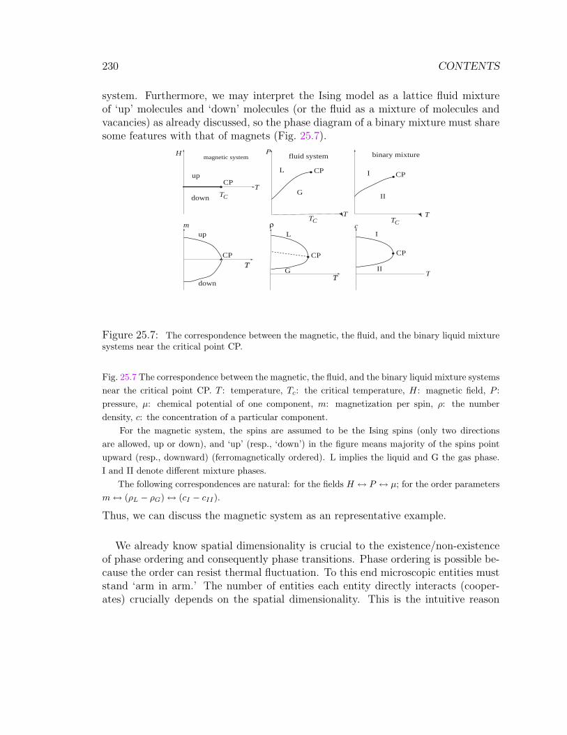
230 CONTENTS
system. Furthermore, we may interpret the Ising model as a lattice fluid mixtureof ‘up’ molecules and ‘down’ molecules (or the fluid as a mixture of molecules andvacancies) as already discussed, so the phase diagram of a binary mixture must sharesome features with that of magnets (Fig. 25.7).
T
T
H P
TC
TC
magnetic system
L
G
CP
fluid system
T
μ
TC
I
II
CP
binary mixture
T
cI
II
ρ
T
L
G
CP CP
T
up
down
CP
m
CPup
down
Figure 25.7: The correspondence between the magnetic, the fluid, and the binary liquid mixturesystems near the critical point CP.
Fig. 25.7 The correspondence between the magnetic, the fluid, and the binary liquid mixture systemsnear the critical point CP. T : temperature, Tc: the critical temperature, H: magnetic field, P :pressure, µ: chemical potential of one component, m: magnetization per spin, ρ: the numberdensity, c: the concentration of a particular component.
For the magnetic system, the spins are assumed to be the Ising spins (only two directionsare allowed, up or down), and ‘up’ (resp., ‘down’) in the figure means majority of the spins pointupward (resp., downward) (ferromagnetically ordered). L implies the liquid and G the gas phase.I and II denote different mixture phases.
The following correspondences are natural: for the fields H ↔ P ↔ µ; for the order parametersm↔ (ρL − ρG)↔ (cI − cII).
Thus, we can discuss the magnetic system as an representative example.
We already know spatial dimensionality is crucial to the existence/non-existenceof phase ordering and consequently phase transitions. Phase ordering is possible be-cause the order can resist thermal fluctuation. To this end microscopic entities muststand ‘arm in arm.’ The number of entities each entity directly interacts (cooper-ates) crucially depends on the spatial dimensionality. This is the intuitive reason
25. LECTURE 25: SPATIAL DIMENSIONALITY AND INTERACTION RANGE ARE CRUCIAL231
why spatial dimensionality matters,Let us look at the effect of spatial dimensionality on the Ising model.
1-Ising model: We can obtain the free energy (with magnetic field) exactly as wewill see later by, e.g., the transfer matrix method; the phase transition does not occurfor T > 0 as we have intuitively seen above (Peierls’ argument).148
2-Ising model: (1) The Onsager solution gives the free energy without magneticfield.149 There is a phase transition at Tc > 0 as we already know.(2) Below the phase transition temperature Tc there are only two phases correspond-ing to the up spin phase and the down spin phase, and there is no phase coexis-tence.150 That is, up and down phases cannot coexist (see Fig. 25.8).
+ ++ +
++ ++ +
+
++
++
++
_ _ _ _
_
___
__
__
_ _ _ _
+_
__
__
++
Figure 25.8: Even the half up and half down fixed boundary spin configuration cannot stabilizethe interface location between up and down phases for 2D Ising model below Tc.
Fig. 25.8 Even the half up and half down fixed boundary spin configuration cannot stabilize theinterface location between up and down phases for 2D Ising model below Tc. The interface may beunderstood as a trajectory of a Brownian particle connecting the two phase boundary points at theboundary (Brownian bridge). If the system size is L, then its amplitude is
√L. In the thermody-
namic limit almost surely the observer at a fixed point (say, at the center) who can observe only afinite volume can observe only one of the phases, and can never see the spin flip in her lifetime.
(3) Near Tc there are various nontrivial critical divergences.151
3-Ising model: (1) No exact evaluation of the free energy is known, but it is easyto demonstrate that Tc > 0 (see Peierls’ argument). It is known that at sufficientlylow temperatures there are phase coexistence.152
148It is not hard to show that T = 0 is a phase transition point for this model.149due to L. Onsager.150Independently due to M. Aizenman and Y. Higuchi.151Here, ‘non-trivial’ means that the fluctuation is so large that we cannot use mean-field theory
to study the divergent behavior correctly.152due to R. L. Dobrushin
232 CONTENTS
(2) The critical divergences are non-trivial just as in 2-space.
Beyond 3-space: Although no exact free energy is known, the existence of positiveTc is easy to demonstrate, and the critical divergences around this point are believedto be the same for all d ≥ 4. This has been established for the dimension strictlygreater than 4.153
153due to M. Aizenman. 4-Ising model still defies mathematical studies.
26. LECTURE 26: WHY CRITICAL PHENOMENA ARE DIFFICULT; MEAN-FIELD THEORY233
26 Lecture 26: Why critical phenomena are diffi-
cult; mean-field theory
Summary∗ How order is lost upon changing T is discussed.∗ It is explained why the second order phase transition is difficult to study.∗ To understand the phase diagram we need renormalization group and mean-fieldtheory.∗ The mean field theory is formulated with the aid of conditional expectations.
Key wordscorrelation length, central limit theorem, renormalization group, (genuine and triv-ial) universality, mean-field theory, bifurcation.
What you should be able to do∗ You must be able to illustrate what happens if you approach a second order phasetransition by changing T .∗ You must be able to set us the mean-field equation. There are many ways, but theformulation in terms of the conditional probability is the most elegant, so memorizethe approach.∗ You should know qualitative feature of tanh x.∗ How to solve (or qualitatively understand) mean-field equation graphically.
Let us review what we did last week.
What is the phase transition? If a thermodynamic variable is varied and if amathematical singularity (loss of continuity, loss of differentiability, etc.; loss of an-alyticity in short) in a thermodynamic potential is observed, we say there is a phasetransition. That is, a phase transition is characterized by a mathematical singularityof a thermodynamic potential.
The existence of a singularity requires a very large system (strictly speaking, aninfinitely large system). Thus, to formulate singularities mathematically, we needthe thermodynamic limit. In the thermodynamic limit extensive quantities are allinfinite, so we define thermodynamic densities (extensive quantities per particle). Aphase transition may also be characterized by a mathematical singularity of a ther-
234 CONTENTS
modynamic density.We have seen that statistical mechanics can describe phase transitions. Peierls
demonstrated that the Ising model in d (≥ 2)-space can order: the magnetizationbecomes non-zero. We have also computed the 1D Kac-model (' van der Waalsfluid).
Phase transitions are often studied by changing intensive parameters (e.g., tem-perature and pressure). When two phases coexist, they share the same intensiveparameters (fields). Therefore, a convenient thermodynamic potential is the general-ized Gibbs free energy for a given amount of material (N); for example, that obtainedby Legendre transformation of internal energy with respect to entropy, volume, mag-netization, etc., except for the number of particles N . The Gibbs free energy maylose differentiability with respect to its natural independent variables (intensive pa-rameters, which is often called fields as mentioned already).154 If the differentiabilityis lost, we say a first order phase transition occurs. If the singularity in Gibbs freeenergy is less drastic, generally we say there is a second order phase transition.155
Let us consider how an order is lost upon changing temperature. If somethingcatastrophic (cooperative loss of order) is the trigger of phase transition, it is likelya first order phase transition.156 If something ‘bad’ happens locally in the solid,there is a domino effect of order deterioration, and quickly the whole system losesthe order. As we discussed before, first order phase transition is a ‘premature’ lossof order.
As a typical second order phase transition, let us consider the Ising model. Letus approach the phase transition from the high temperature side. Up and downspin islands grow as T is reduced (see Fig. 26.1; the figure is constructed using
154G must be continuous. Why?155There is an infinite order phase transition, where G maintains to be C∞ (infinite-times differ-
entiable) but loses analyticity, that is, formal Taylor expansion ceases to converge. This actuallyhappens in 2D XY model. Also such a singularity occurs between the stable and metastablebranches of the free energy.
156The Lindemann criterion illustrates this point; although the phase transition is determinedby the equilibrium condition of the chemical potentials in the ordered and the disordered phases,instability in the ordered phase is sufficiently close to the equilibrium order-disorder phase transitionpoint in the solid-liquid phase transition case.
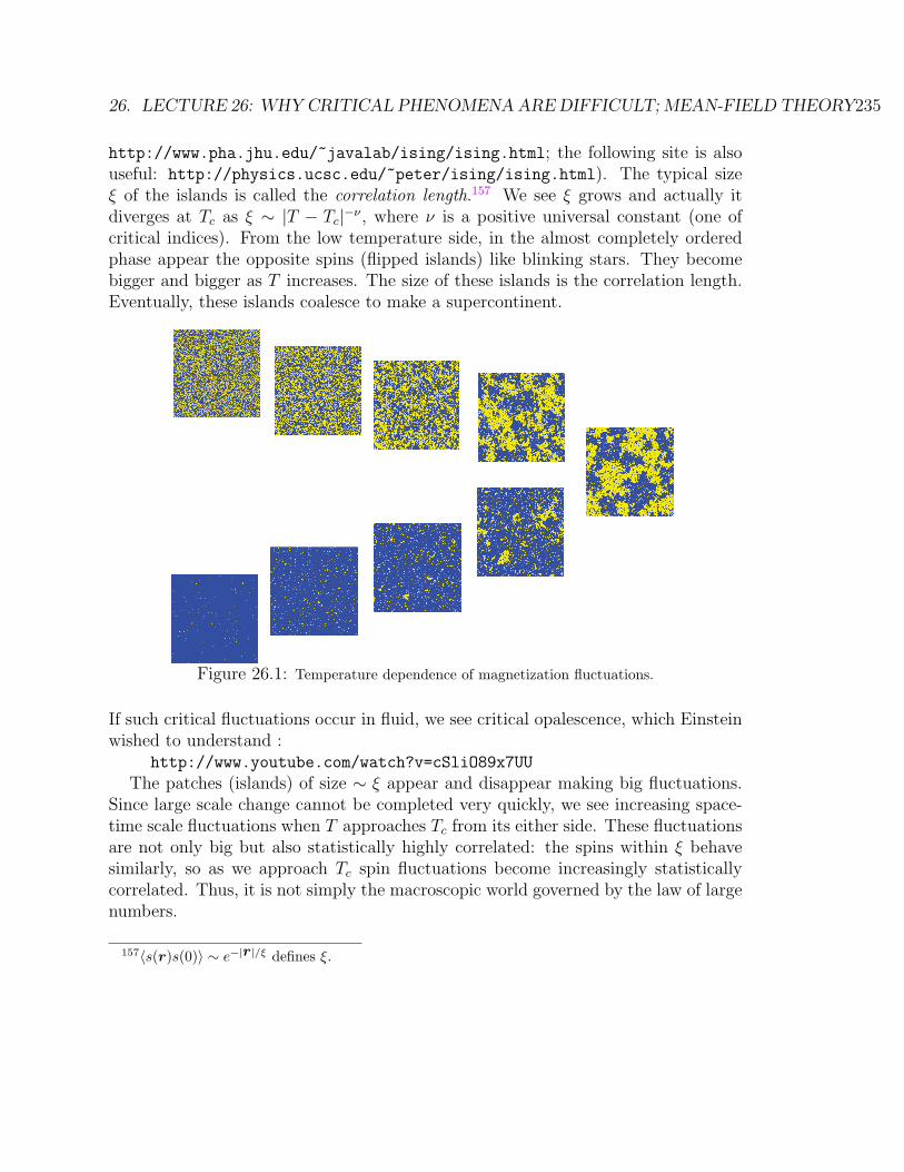
26. LECTURE 26: WHY CRITICAL PHENOMENA ARE DIFFICULT; MEAN-FIELD THEORY235
http://www.pha.jhu.edu/~javalab/ising/ising.html; the following site is alsouseful: http://physics.ucsc.edu/~peter/ising/ising.html). The typical sizeξ of the islands is called the correlation length.157 We see ξ grows and actually itdiverges at Tc as ξ ∼ |T − Tc|−ν , where ν is a positive universal constant (one ofcritical indices). From the low temperature side, in the almost completely orderedphase appear the opposite spins (flipped islands) like blinking stars. They becomebigger and bigger as T increases. The size of these islands is the correlation length.Eventually, these islands coalesce to make a supercontinent.
Figure 26.1: Temperature dependence of magnetization fluctuations.
If such critical fluctuations occur in fluid, we see critical opalescence, which Einsteinwished to understand :
http://www.youtube.com/watch?v=cSliO89x7UU
The patches (islands) of size ∼ ξ appear and disappear making big fluctuations.Since large scale change cannot be completed very quickly, we see increasing space-time scale fluctuations when T approaches Tc from its either side. These fluctuationsare not only big but also statistically highly correlated: the spins within ξ behavesimilarly, so as we approach Tc spin fluctuations become increasingly statisticallycorrelated. Thus, it is not simply the macroscopic world governed by the law of largenumbers.
157〈s(r)s(0)〉 ∼ e−|r|/ξ defines ξ.
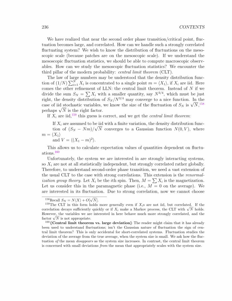
236 CONTENTS
We have realized that near the second order phase transition/critical point, fluc-tuation becomes large, and correlated. How can we handle such a strongly correlatedfluctuating system? We wish to know the distribution of fluctuations on the meso-scopic scale (because patches are on the mesoscopic scale). If we understand themesoscopic fluctuation statistics, we should be able to compute macroscopic observ-ables. How can we study the mesoscopic fluctuation statistics? We encounter thethird pillar of the modern probability: central limit theorem (CLT).
The law of large numbers may be understood that the density distribution func-tion of (1/N)
∑Ni=1Xi is concentrated to a single point m = 〈X1〉, if Xi are iid. Here
comes the other refinement of LLN: the central limit theorem. Instead of N if wedivide the sum SN =
∑Xi with a smaller quantity, say N3/4, which must be just
right, the density distribution of SN/N3/4 may converge to a nice function. In the
case of iid stochastic variables, we know the size of the fluctuation of SN is√N ,158
perhaps√N is the right factor.
If Xi are iid,159 this guess is correct, and we get the central limit theorem:
If Xi are assumed to be iid with a finite variation, the density distribution func-tion of (SN − Nm)/
√N converges to a Gaussian function N(0, V ), where
m = 〈X1〉and V = 〈(X1 −m)2〉.
This allows us to calculate expectation values of quantities dependent on fluctu-ations.160
Unfortunately, the system we are interested in are strongly interacting systems,so Xi are not at all statistically independent, but strongly correlated rather globally.Therefore, to understand second-order phase transition, we need a vast extension ofthe usual CLT to the case with strong correlations. This extension is the renormal-ization group theory. Let Xi be the ith spin. Then, M =
∑Xi is the magnetization.
Let us consider this in the paramagnetic phase (i.e., M = 0 on the average). Weare interested in its fluctuation. Due to strong correlation, now we cannot choose
158Recall SN = N〈X〉+ O[√
N ].159The CLT in this form holds more generally even if Xis are not iid, but correlated. If the
correlation decays sufficiently quickly or if Xi make a Markov process, the CLT with√
N holds.However, the variables we are interested in here behave much more strongly correlated, and thefactor
√N is not appropriate.
160〈〈Central limit theorem vs. large deviation〉〉 The reader might claim that it has alreadybeen used to understand fluctuations; isn’t the Gaussian nature of fluctuation the sign of cen-tral limit theorem? This is only accidental for short-correlated systems. Fluctuation studies thedeviation of the average from the true average, when the system size is small. We ask how the fluc-tuation of the mean disappears as the system size increases. In contrast, the central limit theoremis concerned with small deviations from the mean that appropriately scales with the system size.
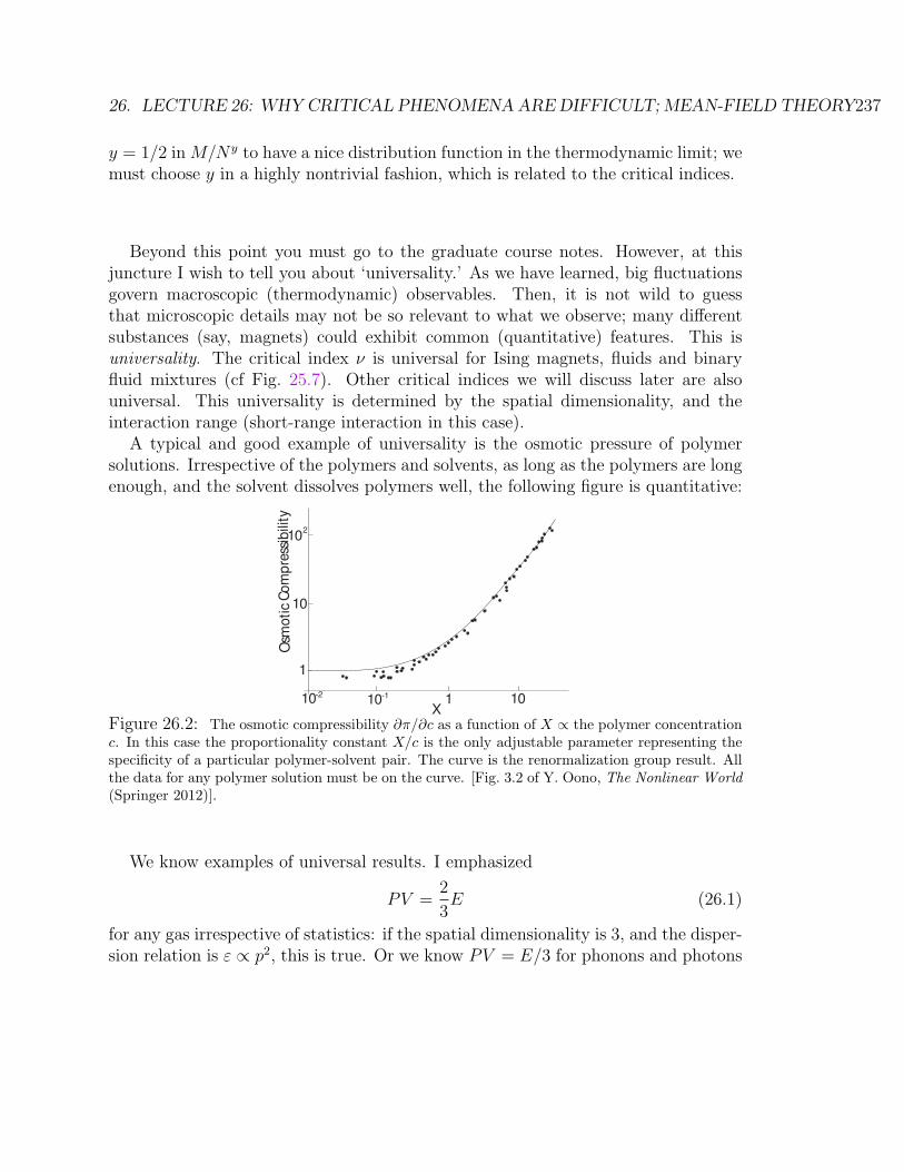
26. LECTURE 26: WHY CRITICAL PHENOMENA ARE DIFFICULT; MEAN-FIELD THEORY237
y = 1/2 in M/Ny to have a nice distribution function in the thermodynamic limit; wemust choose y in a highly nontrivial fashion, which is related to the critical indices.
Beyond this point you must go to the graduate course notes. However, at thisjuncture I wish to tell you about ‘universality.’ As we have learned, big fluctuationsgovern macroscopic (thermodynamic) observables. Then, it is not wild to guessthat microscopic details may not be so relevant to what we observe; many differentsubstances (say, magnets) could exhibit common (quantitative) features. This isuniversality. The critical index ν is universal for Ising magnets, fluids and binaryfluid mixtures (cf Fig. 25.7). Other critical indices we will discuss later are alsouniversal. This universality is determined by the spatial dimensionality, and theinteraction range (short-range interaction in this case).
A typical and good example of universality is the osmotic pressure of polymersolutions. Irrespective of the polymers and solvents, as long as the polymers are longenough, and the solvent dissolves polymers well, the following figure is quantitative:
10 10 10
1
1
10
102
-2 -1
X
Osm
oti
c C
om
pre
ssib
ility
Figure 26.2: The osmotic compressibility ∂π/∂c as a function of X ∝ the polymer concentrationc. In this case the proportionality constant X/c is the only adjustable parameter representing thespecificity of a particular polymer-solvent pair. The curve is the renormalization group result. Allthe data for any polymer solution must be on the curve. [Fig. 3.2 of Y. Oono, The Nonlinear World(Springer 2012)].
We know examples of universal results. I emphasized
PV =2
3E (26.1)
for any gas irrespective of statistics: if the spatial dimensionality is 3, and the disper-sion relation is ε ∝ p2, this is true. Or we know PV = E/3 for phonons and photons
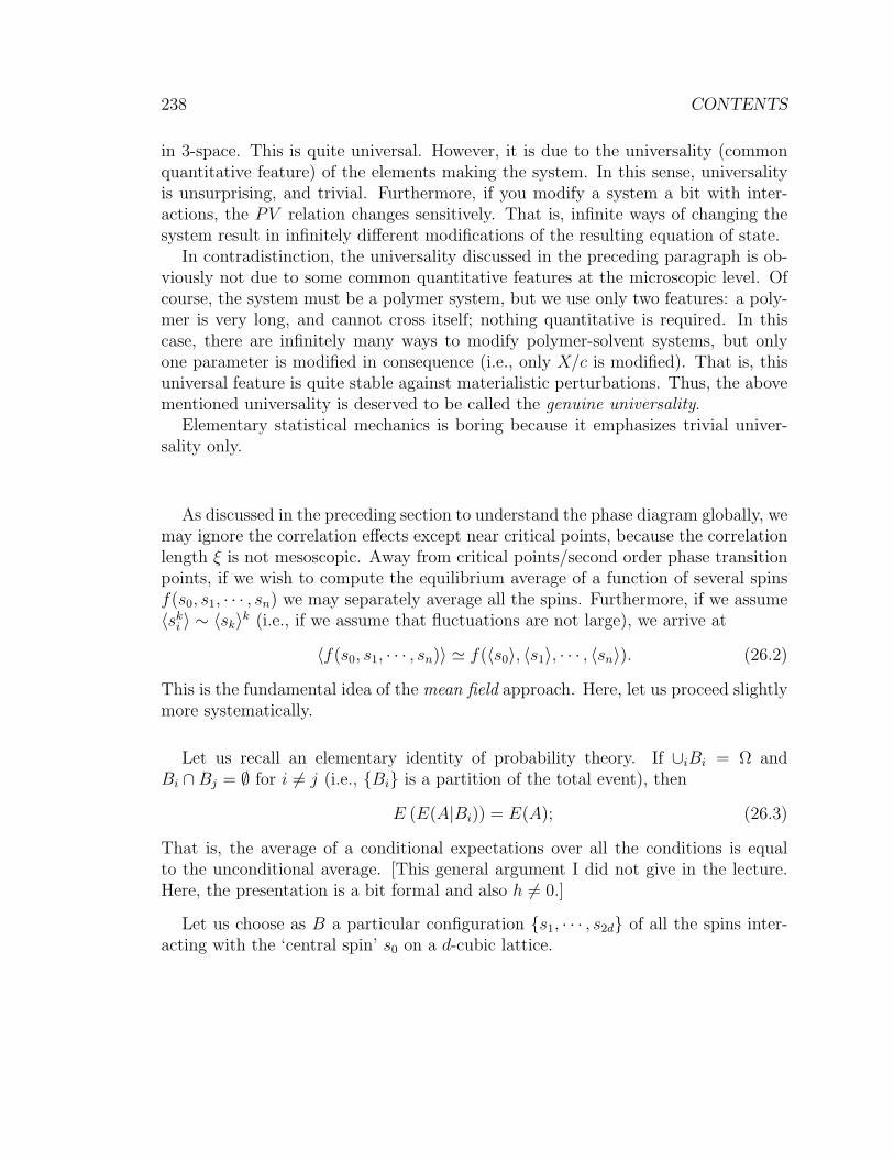
238 CONTENTS
in 3-space. This is quite universal. However, it is due to the universality (commonquantitative feature) of the elements making the system. In this sense, universalityis unsurprising, and trivial. Furthermore, if you modify a system a bit with inter-actions, the PV relation changes sensitively. That is, infinite ways of changing thesystem result in infinitely different modifications of the resulting equation of state.
In contradistinction, the universality discussed in the preceding paragraph is ob-viously not due to some common quantitative features at the microscopic level. Ofcourse, the system must be a polymer system, but we use only two features: a poly-mer is very long, and cannot cross itself; nothing quantitative is required. In thiscase, there are infinitely many ways to modify polymer-solvent systems, but onlyone parameter is modified in consequence (i.e., only X/c is modified). That is, thisuniversal feature is quite stable against materialistic perturbations. Thus, the abovementioned universality is deserved to be called the genuine universality.
Elementary statistical mechanics is boring because it emphasizes trivial univer-sality only.
As discussed in the preceding section to understand the phase diagram globally, wemay ignore the correlation effects except near critical points, because the correlationlength ξ is not mesoscopic. Away from critical points/second order phase transitionpoints, if we wish to compute the equilibrium average of a function of several spinsf(s0, s1, · · · , sn) we may separately average all the spins. Furthermore, if we assume〈sk
i 〉 ∼ 〈sk〉k (i.e., if we assume that fluctuations are not large), we arrive at
〈f(s0, s1, · · · , sn)〉 ' f(〈s0〉, 〈s1〉, · · · , 〈sn〉). (26.2)
This is the fundamental idea of the mean field approach. Here, let us proceed slightlymore systematically.
Let us recall an elementary identity of probability theory. If ∪iBi = Ω andBi ∩Bj = ∅ for i 6= j (i.e., Bi is a partition of the total event), then
E (E(A|Bi)) = E(A); (26.3)
That is, the average of a conditional expectations over all the conditions is equalto the unconditional average. [This general argument I did not give in the lecture.Here, the presentation is a bit formal and also h 6= 0.]
Let us choose as B a particular configuration s1, · · · , s2d of all the spins inter-acting with the ‘central spin’ s0 on a d-cubic lattice.
26. LECTURE 26: WHY CRITICAL PHENOMENA ARE DIFFICULT; MEAN-FIELD THEORY239
sss
ss0 1
2
3
4
Figure 26.3: The central spin s0 and its nearest neighbor surrounding spins s1, · · · , s2d.
We can compute the following conditional average for the d-Ising model on the (hy-per)cubic lattice exactly:
E(s0|s1, · · · , s2d) =
∑s0s0e
βJs0(s1+···+s2d)+βhs0∑s0eβJs0(s1+···+s2d)+βhs0
= tanh[βh+βJ(s1+· · ·+s2d)]. (26.4)
Because E(s0) = E (E(s0|s1, · · · s2d)), we obtain
〈s0〉 = 〈tanh [βh+ βJ(s1 + · · ·+ s2d)]〉. (26.5)
This is an exact relation into which we may introduce various approximations toconstruct mean field approaches.
Now, to compute the RHS of (26.5), we must introduce some approximation. Themost popular (and simple-minded) version is (26.2):
〈tanh[βh+ βJ(s1 + · · ·+ s2d)]〉 ' tanh[βh+ βJ〈s1 + · · ·+ s2d〉]. (26.6)
Therefore, for m = 〈s0〉, we obtain a closed equation
m = tanh[β(2dJm+ h)]. (26.7)
2dJm may be understood as an effective field acting on s0, so this is called the meanfield (sometimes called the molecular field as well). This is the etymology of thename of the approximation method being considered.
Let 2dβJm = x. (26.7) reads
x = 2dβJ tanh(x+ βh). (26.8)
For simplicity, let us assume h = 0. We have to solve
x = 2dβJ tanh x. (26.9)
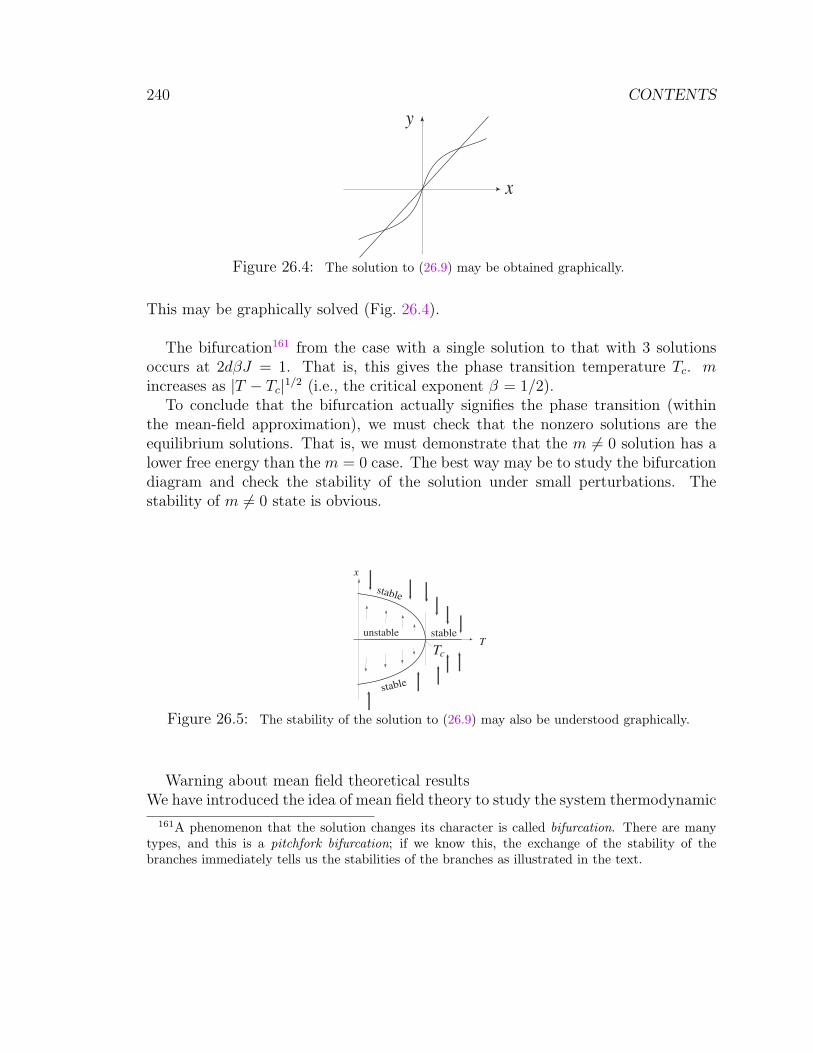
240 CONTENTS
x
y
Figure 26.4: The solution to (26.9) may be obtained graphically.
This may be graphically solved (Fig. 26.4).
The bifurcation161 from the case with a single solution to that with 3 solutionsoccurs at 2dβJ = 1. That is, this gives the phase transition temperature Tc. mincreases as |T − Tc|1/2 (i.e., the critical exponent β = 1/2).
To conclude that the bifurcation actually signifies the phase transition (withinthe mean-field approximation), we must check that the nonzero solutions are theequilibrium solutions. That is, we must demonstrate that the m 6= 0 solution has alower free energy than the m = 0 case. The best way may be to study the bifurcationdiagram and check the stability of the solution under small perturbations. Thestability of m 6= 0 state is obvious.
x
Tc
Tstable
stable
stable
unstable
Figure 26.5: The stability of the solution to (26.9) may also be understood graphically.
Warning about mean field theoretical resultsWe have introduced the idea of mean field theory to study the system thermodynamic
161A phenomenon that the solution changes its character is called bifurcation. There are manytypes, and this is a pitchfork bifurcation; if we know this, the exchange of the stability of thebranches immediately tells us the stabilities of the branches as illustrated in the text.
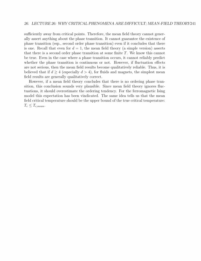
26. LECTURE 26: WHY CRITICAL PHENOMENA ARE DIFFICULT; MEAN-FIELD THEORY241
sufficiently away from critical points. Therefore, the mean field theory cannot gener-ally assert anything about the phase transition. It cannot guarantee the existence ofphase transition (esp., second order phase transition) even if it concludes that thereis one. Recall that even for d = 1, the mean field theory (a simple version) assertsthat there is a second order phase transition at some finite T . We know this cannotbe true. Even in the case where a phase transition occurs, it cannot reliably predictwhether the phase transition is continuous or not. However, if fluctuation effectsare not serious, then the mean field results become qualitatively reliable. Thus, it isbelieved that if d ≥ 4 (especially d > 4), for fluids and magnets, the simplest meanfield results are generally qualitatively correct.
However, if a mean field theory concludes that there is no ordering phase tran-sition, this conclusion sounds very plausible. Since mean field theory ignores fluc-tuations, it should overestimate the ordering tendency. For the ferromagnetic Isingmodel this expectation has been vindicated. The same idea tells us that the meanfield critical temperature should be the upper bound of the true critical temperature:Tc ≤ Tc,mean.

Index
absolute entropy, 155absolute temperature, 84adiabat, 82adiabatic cooling, 110adiabatic process, 80adiabatic wall, 80Aristotelian physics, 15Aristotle (384-322 BCE), 15asymptotic equipartition, 141atmospheric pressure, 16atomism, 5atoms, 5Avogadro’s hypothesis, 18Avogadro, A. (1776-1856), 18
Bernoulli’s equation, 20, 39Bernoulli, D. (1700-1782), 17Brnoulll, J (1654-1705), 30bifurcation, 240binary mixture, 230binomial theorem, 137Boltzmann factor, 40Boltzmann, L (1844-1906), 70Bose-Einstein distribution, 169Bose-Einstein condensation, 184Bose-Einstein distriubtion, 171boson, 168Boyle, Robert (1627-1691), 16Braun, K. F. 1850-1918, 117Brownian motion, 11Buys-Ballot, C H D (1817-1890), 41
Cannizzaro, S (1826-1910), 18canonical partition function, 136Casimir effect, 190cell, 6cell theory, 6central limit theorem, 236Charles’ law, 18Chebyshev’s inequality, 32chemical potential, 79chemical reaction, 118Clapeyron-Clausius relation, 218classical gas, 147Clausius, R (1822-1888), 18Clausius’ inequality, 87Clausius’ law, 80coexistence curve, 217complex systems, 7condensate, 185conditional probability, 25convex curve, 100correlation length, 235covariance, 29covariance matrix, 208critical divergence, 231critical fluctuation, 202
Dalton, J. (1766-1844), 18Democritus, 5density of states, 175density operator, 163detailed balance, 118
257
258 INDEX
diffusion equation, 45, 57dimensional analysis, 7, 47Dulong-Petit’s law, 157
Einstein, 202Einstein, A (1879-1955), 56, 70Einstein’s relation, 57elementary event, 22Empedocles (ca 490-430 BCE), 15end-to-end distance, 54ensemble, 143entropic elasticity, 109entropy, 84entropy maximization principle, 84, 87Epicurus, 6equipartition of energy, 156event, 22expectation value, 27extensive quantity, 69
Fenchel’s equality, 101Fermi energy, 180Fermi level, 173Fermi-Dirac distribution, 171fermion, 168ferromagnetic phase transition, 220Fick’s law, 56first order phase transition, 234fluctuation, 11, 205fluctuation-dissipation relation, 13, 65fluctuation-response relation, 200flux, 44Fourier transformation, 38fourth law, 74free electron gas, 179Frenkel defect, 144
Galileo Galilei (1564-1642), 15gambler’s fallacy, 31
Gay-Lussac, J. L. (1778-1850), 18generalized canonical partition function,
200generalized Gibbs free energy, 234generating function, 38Gibbs paradox, 149Gibbs phase rule, 218Gibbs relation, 84Gibbs-Duhem relation, 118Gibbs-Helmholtz formula, 137Gouy, L G (1854-1926), 50Green-Kubo formula, 213Green-Kubo relation, 211
harmonic system, 161Helmholtz free energy, 98hole, 173
iid, 31independence, 27information, 162intensive quantity, 69internal energy, 67, 78intrinsic heat bath, 140ionization potential, 197Ising model, 220
Jacobian technique, 106Joule-Thomson experiment, 19Joule-Thomson effect, 19Joule-Thomson process, 19
Kac potential, 228Kelvin’s law, 80
Langevin equation, 11Laplace transformation, 38Laplacian, 58large deviation function, 61large deviation principle, 12
INDEX 259
lattice gas, 222law of combining volume, 18law of partial pressure, 18Le Chatelier’s principle, 116Le Chatelier, H. L. 1850-1936, 116Le Chatelier-Braun’s principle, 117Legendre transformation, 99, 100Leucippus (5th c, BCE), 5Lindemann criterion, 234Loschmidt, J J (1821-1895), 70
mass action, 78Maxwell, J C (1831-1879), 17Maxwell’s distribution, 38, 129Maxwell’s relation, 106Maxwell’s rule, 226Maxwell’s relation in terms of Jacobian,
108Mayer’s cycle, 89Mayer’s relation, 89mean field, 238mean field theory, reliability, 240mean free path, 41mean free time, 48megaeukaryote, 7mesoscopic scale, 56mode, 190Monte Carlo integration, 33, 34
Nernst’s law, 154no-ghost principle, 7nuclear spin, 197
Onsager coefficient, 209Onsager solution, 231Onsager’s principle, 209Onsager’s reciprocity relation, 212Onsager’s regression hypothesis, 11Onsager-Machlup-Hashitsume formalism,
13
open system, 78order parameter, 223order-disorder phase transition, 220
partial sum, 31partition function, 11Pascal, B (1623-1662), 16Pauli exclusion principle, 168Peierls’ argument, 224phase diagram, 214phase transition, 215, 233phenomenological approach, 73phonon, 190photon, 190, 192Planck M (1858-1947), 70Planck’s law, 80Planck’s radation formula, 192Poincare, H (1854-1912), 50Poison’s relation, 90polarization vector, 192polymer, 54principle of equal probability, 141probability, 23Protagoras, 7
quadratic Hamiltonian, 190quasistatic process, 75
random variable, 27random walk, 53rate function, 61redundancy, 8regression hypothesis, 59reificationism, 16renormalization group theory, 236reservoir, 86response, 199rotational motion, 197
sample space, 22
260 INDEX
Schottky defect, 132Schottky type specific heat, 133second law, 80second order phase transition, 234sedimentation equilibrium, 40Shannon’s formula, 162shear viscosity, of gas, 47sign convention, of energy exchange, 79Sinai billiard, 8Smoluchowski equation, 66spin-statistics relation, 168stability of matter, 178standard deviation, 28state function, 76statistical independence, 29Stefan-Boltzmann law, 195Stirling’s formula, 132stochastic variable, 27surprisal, 162
temperature, 76thermal contact, 76thermal equilibrium, 73, 76thermal motion, 6thermodynamic degrees of freedom, 218thermodynamic density, 233thermodynamic limit, 11, 221thermodynamic space, 74third law, 155, 157throttling process, 19Tonks’ gas, 229Torricelli, E (1608-1647), 16total mechanical energy, 67transport coefficient, 45transport phenomenon, 44triple point, 217
ultrafine structure, 197universality, 237
vacuum, 16van der Waals, 225van der Waals, J D (1937-1923), 48van der Walls equation of state, 225van Hove volume, 68variance, 28von Guericke, O (1602-1686), 16
work coordinates, 74work, required to create fluctuations, 206
Zermelo E (1871-1953), 70