Embed Size (px)
Citation preview
Flow Turbulence Combust (2016) 97:369–399DOI 10.1007/s10494-015-9701-6
Statistical Models of Large Scale Turbulent Flow
J. J. H. Brouwers1,2
Received: 8 April 2015 / Accepted: 29 December 2015 / Published online: 27 January 2016© The Author(s) 2016. This article is published with open access at Springerlink.com
Abstract The Langevin and diffusion equations for statistical velocity and displacement ofmarked fluid particles are formulated for turbulent flow at large Reynolds number for whichLagrangian Kolmogorov K-41 theory holds. The damping and diffusion terms in these equa-tions are specified by the first two terms of a general expansion in powers of C−1
0 whereC0 is Lagrangian based universal Kolmogorov constant: 6 � C0 � 7. The equations enablethe derivation of descriptions for transport by turbulent fluctuations of conserved scalars,momentum, kinetic energy, pressure and energy dissipation as a function of the derivative oftheir mean values. Except for pressure and kinetic energy, the diffusion coefficients of theserelations are specified in closed-form with C−1
0 as constant of proportionality. The relationsare verified with DNS results of channel flow at Reτ = 2000. The presented results canserve to improve or replace the diffusion models of current CFD models.
Keywords Langevin equation · Diffusion equation · Anisotropic turbulence · Kolmogorovtheory
1 Introduction
A general statistical description of turbulent flow has yet to be delivered [1, 2]. What isknown are partial results: see e.g. [1, 3]. Renowned are the descriptions of the statisticalstructure of the viscous and inertial subrange scales of turbulence according to the similarity
� J. J. H. [email protected]
1 Department of Mechanical Engineering, Eindhoven University of Technology, Eindhoven,The Netherlands
2 Department of Molecular Physics, National Research Nuclear University MEPhI, Moscow,Russian Federation
370 Flow Turbulence Combust (2016) 97:369–399
theory of Kolmogorov, Obukhov and co-workers: see [1], vol. II, ch. 8. Several aspectsof this theory have in the mean time been confirmed by experiment [1, 4], theory [5] anddirect numerical simulations (DNS) of the Navier-Stokes equations [3]. This includes theLagrangian version of Kolmogorov K-41 similarity theory which is of particular interest tothe present analysis. Studies in the past decade confirm several of the universal statisticalproperties of Lagrangian Kolmogorov Theory [6–9].
Kolmogorov theory provides a solid basis for the statistical description of the smallscales. However, it does not give an answer on how to describe the statistical variables gov-erned by the large scales such as velocities, temperature and admixture dispersion which isthe focus of the present analysis. One aspect of Kolmogorov similarity theory which makesit important for the description of the large scale variables is that it yields a connection at theinertial subrange. To be consistent with the statistical structure of turbulence as a whole, sta-tistical descriptions of the large scale variables preferably match with the inertial subrangerepresentations of Kolmogorov theory.
Statistical models for the large-scale variables are less well-established. An old andstill widely used approach is to average the Navier-Stokes equations and to introduce asemi-empirical description for turbulent momentum and scalar transport. It involves imple-menting some form of gradient hypothesis as answer to the closure problem. Proposals ofthe gradient hypothesis date back to the pioneers of turbulence theory: Taylor, Von Karmanand Prandtl [10, 11]. Methods of computational fluid dynamics (CFD) widely used to ana-lyze practical problems of turbulence, notably methods based on the k-ε model, rely onthis approach [12–14]. Its approximate nature is reflected in a number of tunable constantspreceding the gradient hypotheses adopted at various places in these models.
Several approaches have been presented aimed at arriving at a more detailed descriptionof Eulerian-based statistics of the large scales. To mention: Von Karman’s hypothesis ofself-preservation, Millionshchikov’s zero-fourth-order cumulated approximation, Kraich-nan’s direct -interaction approximation and renormalization-group analysis: see [1], vol. II,ch. 7 and [15]. The approaches were applied to averaged Navier-Stokes equations. Theyyielded insights in several aspects of Eulerian statistical turbulence. At the same time theyhave not come to widespread application or implementation in today’s CFD-codes. One ofthe reasons is that the applied approximation schemes could not be linked to a small dimen-sionless parameter or dimensionless number enabling a convergent expansion scheme forgeneral forms of turbulence. Absence of a small parameter was also an obstacle in deriv-ing a solution for the simplest problem of them all: the diffusion equation of a conservedscalar. There were even doubts whether the formulation of the equation is valid altogetherfor general inhomogeneous anisotropic turbulent flow: see [1], vol. I, ch. 10 and [16, 17].Stochastic theory only provides a derivation of the diffusion equation for the theoreticalabstraction of homogeneous turbulence [1, 16, 17].
The formulation of a statistical model on the basis of merely statistical averaging of theNavier-Stokes equations is bound to be difficult. A similar situation is seen in moleculardynamics where derivation of statistical descriptions by averaging Hamiltonian equations ofmotion of the molecules has proven to be a cumbersome and long-lasting process. Insteadstatistical models of molecular motion were already formulated by renowned physicists inthe beginning of 1900 by adoptingMarkov-type of approaches: see e.g. [18–20]. The modelswere specified by arguments of symmetry and general principles of underlying physics, notby solving Hamiltonian dynamics in detail. The precise connection between the statisticalmodels at macro-level and detailed physics at micro-level is even today a not fully resolvedissue [18]. It are the statistical models at macro-level which delivered expressions for the
Flow Turbulence Combust (2016) 97:369–399 371
much used laminar coefficients of viscosity, thermal conductivity and diffusivity in termsof molecular constants: e.g. [19, 21]. Kolmogorov’s similarity theory is an example of anapproach at macro-level. It forms an important anchor in the development of a statisticalmodel of turbulence.
Also in turbulence there is room for a Markov approach. More specifically, a Markovmodel for the velocity of fluid particles. Such a model is consistent with the asymptoticstructure of turbulence at large Reynolds number where correlations of particle accelera-tions becomemore and more δ-related with increasing Reynolds number: e.g. see [1], vol. II,Section 21.5. Moreover the Langevin equation associated with the Markov model matchesthe inertial subrange limit of ordinary (K41) Kolmogorov theory [3]. The effects of (inter-nal) intermittency are disregarded in this approach. This can be justified on grounds that itseffect is limited in the statistics of velocities and displacements. This is apparent from (i)evaluations based on refined Kolmogorov theory, see [1], vol II, Section 25 and [3], Section6.7.5; (ii) from results of fractal models dealing with intermittency [22] and (iii)from themany results of measurements and DNS showing limited deviations from Gaussian behav-ior of velocities [4, 23–26]. In the present analysis we leave the refinement of intermittencyaside. The focus is on a statistical description of the large scale variables which starts fromthe Markov model and which is applicable to configurations of turbulent flow which areotherwise as general as possible.
The Langevin equation is a Lagrangian description of statistical fluid particle motion.It describes velocity while moving with the particle in contrast to the more familiar Eule-rian description employed in fluid dynamics where the fluid velocity is specified at a fixedposition. A first version of the equation appropriate for homogeneous isotropic turbulencewas already formulated by Taylor [27] in 1922. A more general formulation applicable toinhomogeneous anisotropic turbulence was brought forward in the eighties and nineties: seee.g. [3, 16, 28, 29]. Problem however was that the damping function in the equation couldnot be specified in a unique manner. The issue was in part solved by imposing Thomson’swell-mixed condition [16] which provides a match with statistical Eulerian flow. The solu-tion procedure was completed by introducing a perturbation expansion whereby the inverseof the Kolmogorov constant C0 served as small parameter [30–32]. The constant entersinto the Langevin equation through the connection with the inertial subrange representationof Lagrangian Kolmogorov theory. Recent results of Lagrangian based DNS and measure-ments indicate that the value of the universal constant C0 should be somewhere between6 and 7: see [8, 9, 30–32], Ref. [3], p. 504. The C−1
0 -expansion yielded an expression inclosed-form for the damping function in the Langevin equation which enables specificationof particle velocity statistics up to a relative error of O(C−1
0 ). Moreover, through the C−10 -
expansion it was possible to derive a diffusion equation for the position of a marked fluidparticle or passive admixture concentration which is accurate up toO(C−2
0 ). Results agreedwithin the specified bounds of error with values of statistical parameters obtained by DNS,measurement and theory for a number of relevant cases of turbulent flow. A summary ofthis work including some extensions is given in Sections 2–4.
The diffusion equation for the position of a marked fluid particle entails an Eulerian-based description of turbulent transport of a conserved scalar. It was derived from theLangevin equation for statistical fluid particle velocity which is a Lagrangian-based descrip-tion. In this paper we shall elaborate on the Lagrangian-Eulerian connection (see Section 5).We shall use the Lagrangian-based descriptions of statistical particle velocity to deriveEulerian based expressions for turbulent transport of momentum (Sections 6 and 7),and of kinetic energy, pressure and energy dissipation rate (Section 8). Predictions are
372 Flow Turbulence Combust (2016) 97:369–399
verified against results of DNS of turbulent channel flow at Reτ = 2000 [33, 34] (Section 9).Implementation of the results in CFD is discussed in Section 10.
2 Langevin Equation of Fluid Particle Velocity
We consider turbulent flow of an incompressible or almost incompressible fluid, e.g. a liq-uid or a gas flowing at speeds much less then the speed of sound. In accordance withcases of real-life turbulent flow, the Eulerian statistical field is stationary, anisotropic andinhomogeneous in space. Statistical averages of fluctuating flow variables assessed at afixed point in space are constant in time. Their values can be obtained by time-averagingat the point of concern. The thus obtained values vary in space and direction. We denotethe fluid velocity at a fixed point in space, i.e. Eulerian fluid velocity, by ui = ui(x, t)
where i = 1, 2, 3 is direction in space, x is position in space and t is time. Fixed-pointstatistical averages are denoted by angled brackets < >. Fixed-point average of Eule-rian velocity is denoted by ui
0 =< ui(x, t) >= ui0(x), fixed-point mean-square average
of fluctuating velocities u′i (x, t) = ui(x, t) − ui
0(x) by < u′iu
′j >= σij (x) = σij , also
known as Reynolds stress divided by density. Mean energy dissipation rate is denoted byε = ε(x) = 1
2ν < ((∂/∂xj )u′i +(∂/∂xi)u
′j )
2 > where ν is kinematic viscosity and repeatedindices i or j imply summation.
A description is sought for the randommotion of a marked fluid particle or tracer particlewhich moves with the fluid as if it is part of it. Attention is focused to turbulent flow atlarge Reynolds number Re = k1/2L0ν
−1, where k = 12
∑i σii is mean kinetic energy of
fluctuations and L0 is external length scale, e.g. distance from a wall; for L0 we can takek3/2ε−1. When Re >> 1 the statistical descriptions known for large Reynolds turbulencecan be invoked [1]. Effects of intermittency will be disregarded. They are mostly apparentin acceleration statistics but less visible in velocity and displacement statistics [22]. Underthese conditions the statistical velocity of a fluid particle can be conveniently modelledaccording to a Markov process. It obeys a Langevin equation of the form
dv′i
dt= a′
i (v′, x) + (C0ε(x))1/2wi(t), i = 1, 2, 3 (1)
where v′i = v′
i (t) is the statistical representation of fluctuating fluid particle velocity relativeto Eulerian mean velocity u0i (x) evaluated at particle position x = x(t). Velocity is relatedto position by
dxi
dt= u0i (x) + v′
i (2)
In Eq. 1 a′i = a′
i (v′, x) is damping function and wi(t) is Gaussian white noise of unit
intensity. The excitation term in Eq. 1 is in accordance with the inertial sub-range limit ofnon-intermittent Lagrangian Kolmogorov theory with C0 as universal constant: 6<∼C0
<∼7.Descriptions for the damping function can be obtained by employing an expansion pro-
cedure in which C−10 is used as small parameter [30–32]. The procedure is based on the
notion that solutions of the Langevin equation and the Fokker Planck equation associatedwith it will depend on C0. It is assumed that for small values of C−1
0 this dependency can
be captured by describing the solution by a perturbation expansion in powers of C−10 . The
dependency of the variables in the equations on C0 can be based on general scaling rulesof turbulence. It enables to equate terms of equal order in C−1
0 thus resulting in simplifiedequations which specify the separate terms of the expansion which describe the solution.

Flow Turbulence Combust (2016) 97:369–399 373
The basic structure of the perturbation scheme can be inferred from the Kolmogorov-based representation of the white noise term in the Langevin equation [31, 32]. The Eulerianversion of the Fokker Planck equation associated with the Langevin equation describes theprobability distribution of Eulerian velocities [16]. Physically acceptable solutions of thisequation are only obtained if the damping function which is next to the diffusion termbased on Kolmogorov theory does not vanish in the limit procedure C−1
0 → 0 relativeto the diffusion term. For this to happen the damping term must be proportional to C0[31, 32]. This is also the condition for which the Eulerian-based averages of fluctuatingvelocities derived from this equation are to leading order not dependent on C0. These aregoverned by the large scales of turbulence which are determined by the external conditionsof the configuration: [1], Vol.2,sec.21.3.The dominant time scale of fluctuations of particlevelocity and of velocity correlations now follows from Eq. 1 as being proportional to C−1
0 .
These time scales and related scales of particle displacement are a factor C−10 smaller than
the time scale and scales of spatial variation of the Eulerian-based averages which will notdepend on C0. They will scale with L0k
−1/2 and L0, respectively, where L0 is externallength scale of the configuration and where the square root of kinetic energy k is used torepresent the magnitude of the velocity fluctuations. It are these proportionalities or scalingswith respect to C0 which determine the structure of the expansion scheme and which permitapproximation. They rest on general principles of perturbation techniques and scaling lawsof turbulence. The results hold for turbulence for which Lagrangian Kolmogorov theory andthe Langevin model are valid. The accuracy of the results and evidence obtained so far arediscussed in Section 4. The result for the damping function is [31, 32]
a′i = −1
2C0λij εv
′j + 1
2λjmu0k
∂σmi
∂xk
v′j + 1
2λjn
∂σij
∂xm
(v′mv′
n + σmn) + a′iH (3)
where λij = λij (x) = σ−1ij is inverse of the co-variance tensor and where the term a′
iH is
defined and discussed below.The leading linear term in the expression for damping corresponds to a Hamiltonian base
case. The typical time-scale over which velocities fluctuate and over which correlationsbetween velocities decay isC−1
0 L0k−1/2. During such times the displacement of the particle
because of fluctuation is typically C−10 L0. This is small compared to the length scale over
which the Eulerian parameters in the Langevin equation vary when C−10 � 1. In the leading
order formulation with respect to C−10 we thus can assume that the statistical process of
velocity fluctuations takes place in a local homogeneous area of the Eulerian statisticalfield. Furthermore, energy production and dissipation occurs on the time scale kε−1 orL0k
−1/2 which is much larger than the time scale of the velocity process if C−10 � 1. It
gives ground to consider the underlying physics of velocity fluctuations in the leading orderformulation as that of a Hamiltonian process. The formulation of the leading term in thedamping function can then be specified by applying the fluctuation-dissipation theorem andOnsager symmetry.
Hamiltonian behavior and Onsager symmetry can not be required to hold for next-to-leading order formulations, i.e. the second, third and fourth term on the right hand side ofEq. 3. When specifying these terms use has been made of Thomson’s condition of well-mixing with Eulerian flow statistics [16]. Implementation of this condition, however, doesnot lead to complete specification. This is reflected by the presence of the term a′H
i =a′H
i
(v′, x
)in Eq. 3. To satisfy well-mixing a′H
i should satisfy a first order differential
equation in v′ for which a multitude of solutions exist [16, 31, 32]: a′Hi = 0 leads to
a Langevin model proposed by Thomson [16]. What can be said is that according to the
374 Flow Turbulence Combust (2016) 97:369–399
outcome of the C−10 -expansion, whatever the form of a′H
i , its contribution to the damping
term is limited to one of relative magnitude O(C−10 ) compared to the leading linear term.
Its contribution reduces even to one of relative magnitude O(C−20 ) in the description of the
statistics of particle velocity and position on the time-scale of the diffusion limit. This underthe proviso that a′H
i satisfies the well-mixed condition [31, 32].
3 The Diffusion Limit
Statistics of particle displacement can be calculated from time simulations based onEqs. 1–3. A more direct way to describe these statistics is provided by the diffusion equa-tion. It can formally be derived from the Fokker-Planck equation associated with Eqs. 1–3by expanding in powers of C−1
0 and stretching time by C0 [30–32]. An alternative and moreconcise derivation has been presented in the Appendix. The result is the diffusion equationfor mean passive admixture concentration G0 = G0 (x, t), or equivalently the probabil-ity density distribution of marked fluid particles p(x, t) = G0. The probability density isrelated to the joint density of v′ and x by p (x, t) = ∫ ∞
−∞ p(v′, x, t) dv′ where the joint den-sity is determined by the Fokker-Planck equation associated with Eqs. 1–3. The diffusionequation is given by
∂G0
∂t+ u0i
∂G0
∂xi
= ∂
∂xi
(
Dij
∂G0
∂xj
)
(4)
where Dij is turbulent diffusion coefficient
Dij = 2C−10 ε−1σinσnj + 2C−2
0 ε−2σliσjku0n
∂σlk
∂xn
(5)
−4C−20 ε−1σkju
0n
∂
∂xn
(ε−1σimσmk
)
The above descriptions involve a truncation error of relative magnitude O(C−20
)com-
pared to the leading term. Compared to previous results [31, 32] the diffusion coefficientcontains an extra next-to-leading order term, i.e. the third term on the r.h.s. of Eq. 5. It is dueto change in mean flow direction of the leading order term in the diffusion coefficient. This
change was assumed to be smaller thanO(C−10
)and therefore negligibly small in previous
derivations [31, 32]. The extra term makes the specification of next-to-leading order termscomplete.
The second term in the diffusion coefficient stems from the second term in the dampingfunction, cf. Eq. 3. All other terms of next-to-leading order in the damping function, viz. thethird and fourth term in Eq. 3, do not contribute to the same order in the diffusion model.
Their contributions all reduce to relative magnitude O(C−20
). It is a consequence of the
Gaussian structure of the leading order process and of satisfying the well-mixed conditionensuring matching with the Eulerian statistical field: see Appendix.
While the first term in Eq. 5 constitutes a symmetric tensor, the other termsdo not. However, within the approximation scheme of terms up to relative mag-
nitude O(C−20
)the anti-symmetric part can be disregarded. This becomes appar-
ent noting that (∂/∂xi)(Dij
(∂/∂xj
)G0
) = (∂/∂xi)((
Dsij + Da
ij
) (∂/∂xj
)G0
)=
(∂/∂xi)(Ds
ij
(∂/∂xj
)G0
)+
((∂/∂xi) Da
ij
) (∂/∂xj
)G0 where upper-scripts s and a refer to
Flow Turbulence Combust (2016) 97:369–399 375
symmetric and anti-symmetric parts respectively. The anti-symmetric part becomes a con-
vection term. Because the anti-symmetric part isO(C−20
), its relative magnitude compared
to the leading part of the convection term is an order smaller than that specified by the two-term approximation scheme. We thus can make the diffusion coefficient symmetric without
losing accuracy up to and including relative magnitudes of O(C−10
)which is the overall
accuracy of the presented results.In case of uni-directional mean flow such as in developed flow in pipes and channels,
only the leading first term in the diffusion coefficient matters. The second and third termare zero because the Eulerian statistical averages are constant in the direction of the meanflow. For homogeneous decaying turbulence behind a grid the decay will lead to a non-zerovalue of the second term in Eq. 5. The third term, on the other hand, tends to zero in thelimit of large Reynolds number: the combination of parameters ε−1σimσmk happens thento be constant in mean flow direction [31, 32]. When dealing with more general cases ofchanging Eulerian statistical averages in the mean flow direction, e.g. turbulent boundarylayers, jets, wakes, the second and third term in Eq. 5 are both to be taken into account.The second and third term scale as C−1
0 which is in accordance with the Eulerian time scale
kε−1 to be taken for[uo
n (∂/∂xn)]−1. The Eulerian time scale is the scale which applies to a
balance between the convective terms in averaged versions of the Navier-Stokes equations.The balance complies with continuous transfer of energy from large to small scales leadingto Kolmogorov’s hypotheses.
From result (5) it is seen that the diffusion coefficient is proportional to C−10 . The depen-
dency will cause the diffusion term in diffusion equation (4) to vanish when taking the limitC−10 → 0. The anomaly disappears once we stretch the coordinate in mean flow direction
or the time in a frame which moves with the mean flow by the factor C0. This is what isdone in the mathematical procedures leading to the diffusion equation of [31, 32]. The phys-ical interpretation is that although diffusion by turbulence is much larger than diffusion bymolecular motion, it is of limited magnitude compared with convective transport by meanflow. This feature can be observed in turbulent plumes.
4 Evidence of the C−10 -Expansion
Central in the derivation of the Langevin and diffusion equation is the expansion proce-dure based on powers of C−1
0 . The expansion was made possible by the position of C0 asautonomous parameter in the governing equations and the scalings related to it. The param-eter originates from the inertial sub-range limit of the small viscous scales of turbulence.In accordance with ordinary K-41 Kolmogorov theory, with increasing Reynolds number,except from the mean energy dissipation rate, the statistical behavior of the small viscouscontrolled scales of the velocity field decouples from that of the large non-viscid scales ofturbulence where instability governs the flow: see [1],vol.2, Section 21.3. Eulerian-basedstatistical quantities which appear as parameters in the Langevin and Fokker-Planck equa-tions and whose values are governed by the large scales of turbulence, viz. mean fluidvelocity, mean energy dissipation rate and covariance of velocity are determined by theexternal conditions of the flow configuration ([1],vol.2, Section 21.3) and are assumed tobe independent on C0 at leading order. An example where such lack of dependency onC0 can be observed in explicit terms are the exact descriptions and solutions of Langevinand Fokker-Planck equations of decaying turbulence behind a grid: see appendices of [31,32]. In particular cases such as the log-layer of wall-induced turbulence a refinement of the
376 Flow Turbulence Combust (2016) 97:369–399
expansion scheme may be appropriate. This is indicated in the discussion of Fig. 1 in Sec-tion 9 where the dependency on C−1
0 of subsequent terms is rearranged in hindsight usingthe results of the basic expansion.
The C−10 expansion can be executed as a mathematically well-defined perturbation tech-
nique. Subsequent terms decrease in magnitude with C−10 by their dependency on C−1
0 . The
expansion can be subjected to the limit procedure C−10 → 0 leading to limiting situations
which allow physical interpretation. Question is whether the value of C−10 of about 0.15
is small enough to describe variables by a limited number of terms and whether the limit-ing situations which are identified agree with observations. Investigations have yielded thefollowing evidence:
1. In the leading order formulation with respect to C−10 the underlying stochastic process
is locally Hamiltonian implying that the statistical distributions of velocity are Gaussian
to O(C−10
). This is in line with the many results of measurements and DNS obtained
for various cases of turbulence: grid turbulence [23], turbulent pipe and channel flow[24, 25, 33, 34], turbulent boundary layers [26] and turbulence between counter rotatingdisks [4]. They revealed limited values of skewness and kurtosis (= flatness − 3) ofabout 0.4 or less.
2. The concept of locally homogeneous Hamiltonian behavior has been tested againstresults for Lagrangian velocity correlations. The Hamiltonian base case is obtained byimplementing the leading linear representation of damping and taking coefficients con-stant in space in Eqs. 1 and 3. It is then possible to derive from the Langevin equationexpressions in closed-form for velocity correlations. These correlations compare wellwith exact results for decaying grid turbulence [32], with Lagrangian DNS results ofpipe, channel and uniform shear [9, 30, 32] and with Lagrangian based experimentalresults of pipe flow using particle tracking velocimetry [32].
3. Onsager symmetry should hold in the leading order formulation. This is confirmedby a relatively small anti-symmetric part of the cross-correlation functions of particlevelocity found for cases of anisotropic turbulence: viz. pipe and channel flow and non-stationary homogeneous anisotropic shear flow [9, 31, 35]. Results originated fromDNS and particle tracking velocimitry. The anti-symmetric part of the cross-correlationfunctions was not more than 20% of the symmetric part, which is in line with a relative
error ofO(C−10
).
4. Predictions based on the diffusion limit have been verified against results obtainedfrom time-domain simulations using the Langevin equation. This was done for thelog-layer of wall-induced turbulence for which there exist asymptotically exact expres-sions for u0i (x), ε (x) and σij (x). These expressions were implemented in Eqs. 1–3to simulate particle tracks. Their statistics were found to compare favourably with ana-lytical results derived from the corresponding diffusion equation [30]. Deliberatelyintroduced anti-symmetry by giving a′H
i , a non-zero value of O (1)) in the dampingfunction revealed minimal effect on displacement statistics [30]. Furthermore it wasfound that displacement statistics were strongly non-Gaussian because of inhomogene-ity of the coefficients in the Langevin and diffusion equation. Values of skewness andkurtosis of wall-normal displacement amounted to 2 and 6, respectively [30]. It con-trasts with velocity statistics where these parameters of non-Gaussian behavior are lessthen 0.4.
5. Exact formulations exist for the Langevin and diffusion equation of decaying gridturbulence at large Reynolds number: see appendices of [31, 32]. The solutions for
Flow Turbulence Combust (2016) 97:369–399 377
correlation functions and diffusion coefficients derived from these equations can beexpanded for small C−1
0 . It yields the same results as those of the presented expan-
sion method up to and including O(C−10
). The exact result enables to determine the
truncation error in the diffusion coefficient: 49C
−20 . For C0 = 6, this implies an error
of 1.2 % in the diffusion coefficient of Eq. 5. The second term in the diffusion coef-ficient describes the effect of the decay. It contributes by a term of relative magnitude(2/3) C−1
0 compared to unity. It confirms the decreasing contribution of higher orderterms.
6. When dealing with more general cases of changing Eulerian statistical averages in themean flow direction, e.g. turbulent boundary layers, jets, wakes, the second and thirdterm in Eq. 5 describe the effect of the change in the mean flow direction in addi-tion to the basic form of diffusion described by the first term. Verification has yetto come.
7. Lagrangian DNS results of channel flow have been used to determine the wall-normal diffusion coefficient versus wall-normal distance [9]. Results compare well withtheoretical predictions based on Eq. 5.
8. Matching results from the Langevin and diffusion equation with large-Reynolds datafrom external sources consistently yield a value of the Kolmogorov constant which liesbetween 6 and 7 approximately. Data stem from Lagrangian-based DNS and measure-ments of homogeneous grid turbulence [8] and inhomogeneous anisotropic turbulencein channels and pipes [9, 30–32].
9. The expressions for wall-normal diffusion coefficient lead to values of wall-normaltransport of heat and mass which agree with the many experimental results for thesequantities reported over the last 50 years [30].
The predictions based on the results of the C−10 -expansion are in many respects in agree-
ment with the results of theory, measurement and DNS for the various cases of differentturbulent flow which were considered. Deviations are in line with what is to be expectedaccording to the error terms of the expansion schemes. Verification of other cases has yetto come. In the next sections we will extend the diffusion limit to describe diffusion byturbulent fluctuations of fluid momentum, of pressure, of kinetic energy and of energy dissi-pation rate. Here truncation errors for certain variables become larger because of additionalapproximations.
5 Turbulent Transport of a Conserved Scalar: The Lagrangian-EulerianConnection
Omitting diffusion by molecular motion, a passive scalar χ carried by a fluid satisfies theconservation equation
∂χ
∂t+ ∂
∂xi
(uiχ) = 0 (6)
The conserved scalar can be fluctuating concentrations of a passive admixture such assmoke or fumes or fluctuating temperature of an incompressible or almost incompressiblefluid: e.g. a liquid or a gas at subsonic speed. Now average the above equation at a fixedpoint in space and note that 〈χ〉 = G0 is mean concentration. Noting that ui = u0i + u′
i wehave:
∂G0
∂t+ ∂qi
∂xi
= 0 (7)
378 Flow Turbulence Combust (2016) 97:369–399
where
qi = u0i G0 + ⟨u′
iχ⟩
(8)
is average transport of admixture through the surface x = xi . Finding an expression forturbulent transport
⟨u′
iχ⟩as a function of mean statistical values of flow field and mean
concentration is known as the scalar closure problem. The solution is found by connectingEq. 4 with Eqs. 7 and 8:
⟨u′
iχ⟩ = −Dij
∂G0
∂xj
(9)
with a relative error of O(C−20
). It shows that turbulent transport of conserved scalars can
be described in a manner which is analogous to that of molecular diffusion.Equation 9 is the result of connecting the Eulerian-based description of turbulent trans-
port in direction i at the point x according to Eqs. 7 and 8 with the solution according toEq. 4 which originated from Lagrangian-based analysis. In the Lagrangian analysis we areconcerned with trajectories of particles which arrive at the point x = x (0) at time t = 0. Attime t = −τ , τ > 0, the average transport of admixture in direction i can be expressed by
qLi (−τ) = χ (x (−τ) , −τ) ui (x (−τ) ,−τ) (10)
where the overbar denotes Lagrangian averaging, that is, averaging over realisations of par-ticle trajectories. The trajectories all arrive at the same position x = x (0) at time zero withlocal Eulerian velocity ui while being at positions x = x (−τ) at time −τ which are differ-ent for every individual realisation. Trajectories can be simulated by backward integrationof the fluctuation equations of the Langevin model starting from the point x. To complywith passive marking, the starting velocity of each realization is chosen randomly in accor-dance with the Eulerian probability distribution of velocity at the point x. The average valueof a quantity q
(v′, x, t
)at time t follows from adding the calculated values of q
(v′, x, t
)
at time t obtained for every realization and dividing by the number of realizations N whereN is very large. In case of passive admixture of concentration χ or an otherwise conservedscalar, its value is labeled to the fluid particle. Variations in space of χ at time −τ willonly occur because of different particle positions at time −τ for every realization. Underthese circumstances we can replace χ (x (−τ) ,−τ) in Eq. 10 by the distribution of particleposition G0 (x (−τ)) so that
qLi (−τ) = G0 (x (−τ)) u0i (x (−τ)) + G0 (x (−τ)) v′
i (−τ) (11)
where in agreement with the Lagrangian notation of the Langevin equation (cf. Eq. 2) wesubstituted
ui (x (−τ) , −τ) = u0i (x (−τ)) + v′i (−τ) . (12)
For small x (−τ) − x (0), the second term on the r.h.s. of Eq. 11 can be approximatelydescribed by the second term of a Taylor series expansion as
G0 (x (−τ)) v′i (−τ) = ∂G0 (x)
∂xj
(xj (−τ) − xj (0)
)v′i (−τ) (13)
= −∂G0 (x)
∂xj
∫ 0
−τ
v′j (t) v′
i (−τ) dt
We focus now on the description of diffusion in the leading order formulation withrespect to C−1
0 . To leading order in C−10 the coefficients in the Langevin equation can be
taken constant and equal to their values at the point x. It makes the stochastic process
Flow Turbulence Combust (2016) 97:369–399 379
of v′ (t) stationary and facilitates shifting time in the correlation functions to the positivedomain so that
∫ 0
−τ
v′j (t) v′
i (−τ) dt =∫ 0
−τ
v′j (t + τ) v′
i (0) dt =∫ τ
0v′j (t1) v′
i (0) dt1 , (14)
with the result that Eq. 11 becomes
qLi (−τ) = G0 (x (−τ)) u0i (x (−τ)) − ∂G0 (x)
∂xj
∫ τ
0v′j (t1) v′
i (0) dt1 , (15)
The diffusion limit now arrives as follows: [35], Sections 6.7 and 6.8. Velocity corre-lations decay on the time scale τc = C−1
0 kε−1. With decreasing C−10 the correlation time
becomes smaller and smaller and the correlation time approaches that of a delta-correlatedprocess. The time-scale of large scale transport which equals kε−1 remains the same withincreasing C−1
0 . We can take τ very large in the calculation of the integral of the correlationfunction while letting τ → 0 in the description of the large scales. More specifically, wecan write
qLi (−τ)||τ |τc,τ→0 = G0 (x) u0i (x) − ∂G0 (x)
∂xj
∫ ∞
0v′j (t1) v′
i (0) dt , (16)
The integral can be evaluated by substituting the leading order solutions for correlationfunctions. It results in the first term of the diffusion coefficient of Eq. 5: 2C−1
0 ε−1σinσnj
[31, 32]. The Eulerian representation of mean transport of admixture or marked particles atthe point x is given by 〈uiχ〉 = uo
i G0 + ⟨u′
iχ⟩, 〈χ〉 = G0. Equating this with the above
result obtained from Lagrangian-based analysis yields the gradient expression of turbulenttransport (cf. Eq.9) to leading order in C−1
0 .In the leading order formulation the area of correlation is treated as homogeneous. It
allowed shifting time in the evaluation of the integral of the correlation functions: cf. Eq. 14.In the next-to-leading order formulation this is no longer allowed. Spatial variations of thecoefficients are to be considered in the Langevin model to calculate diffusion. The some-what more complex procedure which is necessary in this case has been presented in theAppendix. It yields the expression for diffusion of Eq. 5.
The above treatment of turbulent transport through Lagrangian-based representationsbears resemblance with the analysis applied to diffusion by molecular motion: [18],sec.11B5 and [21], Sections 1.4, 9.3 and 17.3. Different in the present case is that we con-sidered the case of an anisotropic stochastic process. Furthermore, we had to deal withinhomogeneity of the turbulent flow field. In diffusion by molecular motion this is muchless of an issue. The area where there is correlation between molecule velocities scaleswith the free molecular length.The Knudsen number Kn relates this length to the externallength scale of the flow configuration and is generally very small. In the present case inho-mogeneity occurs over lengths k3/2ε−1 while particle velocities correlate over distancesC−10 k3/2ε−1. It is C−1
0 which determines the relative size of the locally homogeneous area.
As C−10 is of limited smallness the area which is brought back to a point in the diffusion
approximation is thus comparatively large. Nevertheless as outlined in Section 4, the C−10 -
expansion seems to work well, also in the area of strong inhomogeneity of the log-layer ofwall-induced turbulence [30]. One reason is that correlations decay exponentially. The dif-fusion limit becomes already effective for lengths which exceed the correlation length to alimited extent. Improved accuracy is also obtained by incorporating terms of next-to-leading
order in C−10 , thus reducing errors to O
(C−20
).
380 Flow Turbulence Combust (2016) 97:369–399
6 Turbulent Transport of Momentum
The averaged version of the equation of conservation of momentum of a fluid in Eulerianrepresentation is given by:
∂Mij
∂xj
= − 1
ρ
∂p0
∂xi
(17)
where p0 is mean fluid pressure, ρ fluid density and
Mij =< uiuj > (18)
mean fluid momentum. In Eq. 17 effects of viscosity have been disregarded; in highReynolds number turbulent flow their effects are usually confined to very thin layers alongwalls. A connection to the Lagrangian description of fluid momentum can be made inanalogy with Eq. 10:
MLij (−τ) = ui (x (−τ) , −τ) uj (x (−τ) ,−τ) (19)
where the overbar stands for Lagrangian averaging over realisations of velocities of particleswhich all are at x = x (0) at time zero while being at position x = x (−τ) at time −τ
which is different for every realisation. Particle velocities can be decomposed by their valueaccording to the mean flow and a fluctuating component in accordance with Eq. 2 by which
MLij (−τ) = u0i (x (−τ)) u0j (x (−τ)) + v′
i (−τ) v′j (−τ) + (20)
u0i (x (−τ)) v′j (−τ) + u0j (x (−τ)) v′
i (−τ) .
Analogous to the procedure of Eqs. 11–16, the last two terms in this equation can bedescribed by the diffusion representation when C−1
0 → 0: i.e.
MLij (−τ)||τ |τc,τ→0 = u0i u
0j + v′
i (0) v′j (0) − Djk
∂u0i
∂xk
− Dik
∂u0j
∂xk
. (21)
The Eulerian description of Mij = Mij (x) is given by
Mij = u0i u0j + σij (22)
where σij =⟨u′
iu′j
⟩is co-variance or Reynolds stress divided by density; σij describes the
average momentum by turbulent fluctuations. Equating the r.h.s. of Eqs. 21 and 22 we have
σij = v′i (0) v′
j (0) − Djk
∂u0i
∂xk
− Dik
∂u0j
∂xk
. (23)
The first term on the r.h.s. is extra compared to the results for passive admixture: cf.Eq. 9. Averages of products of concentration fluctuations of passive admixture with v′ atτ = 0 are zero whereas averages of products of velocity fluctuations are not. The presenceof the extra term necessitates the introduction of additional approximations in order to arriveat workable relations. The approximation concerns describing momentum due to gradientsof the mean flow as a perturbation on an isotropic state. Such an approach is also knownfrom analysis of momentum transport by molecular motion [18, 21]. In case of isotropicbehavior we have v′
i (0) v′j (0) = 2
3k0δij , where k0 is kinetic energy of the isotropic state.Equation 23 then becomes
σij = 2
3k0δij − Djk
∂u0i
∂xk
− Dik
∂u0j
∂xk
. (24)
Flow Turbulence Combust (2016) 97:369–399 381
The equation describes the change of the isotropic state due to mean shear. Because of
diffusion coefficients areO(C−10
), changes of the isotropic state are small and the diffusion
coefficients can be evaluated taking for σij the isotropic state. It yields
σij = 2
3k0δij − 8k20
9C0ε
(∂u0i
∂xj
+ ∂u0j
∂xi
)
(25)
The description is analogous to that of molecular momentum in continua. The first termon the right and side of Eq. 25 describes pressure per unit density caused by isotropic turbu-lent fluctuations. The second term stresses per unit density caused by gradients of the meanflow. The stresses are linearly proportional to the gradients with a constant of proportionally8k20/ (9C0ε) being the equivalent of kinematic viscosity of fluids. A linear proportionalitywith a constant of proportionality often called Eddy viscosity has been proposed alreadyin the early stages of turbulence theory [11, 24]. Its validity and the functional form of theconstant describing its spatial dependency has been debated up to to date. The present anal-ysis confirms the linear relationship for the leading order formulation in powers of C−1
0and reveals the functional form of the coefficient, i.e. its dependency on k0 and ε ,withthe inverse Kolmogorov constant as a factor of proportionality. The functional form k20/ε
is identical to that employed in the k–ε model widely used in CFD packages to calculateturbulent flow [13, 14]. In the k–ε model the functional form k2/ε is proceeded by an empir-ical factor Cμ whose value is assessed by matching with results known for the log-layer inwall induced turbulence: Cμ = 0.09. The constant is less than the factor 8/ (9C0) = 0.15obtained when C0 = 6. This may be ascribed to the absence of anisotropy in the linearmodel. The value Cμ = 0.09 is due to matching the linear model to a case of anisotropicflow. This is no longer necessary when the non-linear descriptions of the next section areincluded. A good match with log-layer results is then obtained without a need to adapt thevalue of the factor 8/9C0: see Section 9.
7 Non-Linear Momentum Transport
As implied by Eq. 25, gradients of the mean flow change the co-variance tensor and therebythe isotropic state. Equation 24 from which result (25) has been derived, however, does notonly hold for changes of the isotropic state but of any other state as well. The underlyingreason is that the expression for turbulent diffusion given by Eq. 5 and to be used in Eq. 24was derived on the basis of a local anisotropic equilibrium valid at each spatial positionwhen C−1
0 << 1. It opens the possibility for extending result (25) by iteration: treat σij
according to Eq. 25 as basic state and calculate from Eq. 24 the new state. Collecting terms
toO(C−20
), we have
σij = 2
3k0
[
δij − C−10 s0ij + 2C−2
0 a0ij + 2
3C−20 εk−2
0 u0n∂
∂xn
(ε−2k30
)s0ij
]
(26)
where
u0ij = 4
3
k0
ε
∂u0i
∂xj
, s0ij = u0ij + u0ji , a0ij = s0inu0jn + s0jnu
0in (27)
The third term between brackets in Eq. 26 describes the quadratic contribution of meanvelocity gradients on the change of the isotropic state. The fourth term the contribution ofchanging k0 in the direction of the mean flow.
382 Flow Turbulence Combust (2016) 97:369–399
Subsequent terms in the above expansion have relative magnitudes C−10 u0ij . They will
grow with gradient of the mean flow; the accuracy of the truncated expansion will thendeteriorate. This behavior does not occur in the original expansion for diffusivity, cf. Eq. 5,from which Eq. 26 via Eq. 24 has been derived. Its coefficients do not depend on mean flowgradient but on co-variances. It indicates that in case of large gradients we can improve theaccuracy of Eq. 26 by extending the expansion to higher order. Large mean flow gradientsoccur in the inertial sub-region and log-layer, the region adjacent to the laminar viscousregion near a wall along which fluid flows. Here, turbulence is produced by shear. Pro-duction equals −σij (∂/∂xj )u
0i and is according to the next but leading terms of Eq. 26
proportional to k20C−10 ε−1((∂/∂xj )u
0i )
2; note that the leading isotropic term in Eq. 26 doesnot cause production as (∂/∂xi)u
0i = 0. Taking production and dissipation of equal order
of magnitude, −σij (∂/∂xj )u0i = ε, we find that u0ij scales as C
1/20 . Consecutive terms in
the expansion of Eq. 26 then decrease by powers of C−1/20 instead of C−1
0 and the expan-
sion expels at O(C−10
). To exploit the accuracy of the original expansion for diffusivity
which is accurate to O(C−20
)we extend the expansion for σij by further iteration by two
subsequent terms:− C−3
0 b0ij + 2C−40 c0ij (28)
which has to be added to the terms between square brackets in Eq. 26. In Eq. 28,
b0ij =(4a0ik + s0il s
0lk
)u0jk +
(4a0jk + s0j l s
0lk
)u0ik (29)
c0ij =(b0ik + s0il a
0lk + a0il s
0lk
)u0jk +
(b0jk + s0j l a
0lk + a0j l s
0lk
)u0ik (30)
From Eqs. 26–30 we find for the mean kinetic energy the expression
k = k0
[
1 + 2
3C−20
∑
n
a0nn − 1
3C−30
∑
n
b0nn + 2
3C−40
∑
n
c0nn
]
(31)
which describes the change of the kinetic energy of the isotropic case k0 by anisotropy ofthe turbulent flow field. The implications of the above extension for predictions of σij in thelog-layer of wall-induced turbulence are illustrated in Section 9.2.
The above descriptions for co-variances are the result of expanding σij in powers of C−10
and equating terms of equal magnitude in basic relations (24). An alternative is to solve thesix equations according to Eq. 24 directly for σij with the other variables as parameters.Equation 24 then constitute an algebraic stress model which can be made part of a closed-setof equations for calculating mean values of large scale variables of turbulent flow. But theapproach does not provide an intrinsic improvement to the approximation scheme underly-ing Eq. 24. The scheme is based on a perturbation on isotropic turbulence represented bythe first term on the r.h.s. of Eq. 24. Solutions for σij derived from this equation can beexpected to be accurate only when anisotropy is not to dominant. Such a limitation does notexist for the expansion for diffusion of passive admixture or marked fluid particles whichwas based on a perturbation of a local equilibrium of anisotropic turbulence. The expan-sion for momentum can thus be expected to have a less wider range of validity than thatfor passive admixture whose appropriateness was discussed in Section 4. In Section 9 weshall investigate the accuracy of the momentum expansion for the case of highly anisotropicchannel flow.
Several non-linear models and algebraic stress models for turbulent transport of momen-tum have been presented: see [3], Section 11.9.2 and [13], sec.8.6. They are based on
Flow Turbulence Combust (2016) 97:369–399 383
proposed constitutive relations subject to constraints of a hypothetical nature. It has not beenpossible to relate these models to the present results. Also in the more simple case of tur-bulence in uni-directional flow where turbulent fluctuations are constant in the direction ofthe mean flow (e.g. developed pipe and channel flow), no correspondence with the presentdescriptions has been found.
8 Equations for Kinetic Energy k and Energy Dissipation Rate ε
The previously derived expressions for turbulent transport of conserved scalars and momen-tum contain the unspecified quantities k and ε. Equations which describe these variablescan be derived from the Navier-Stokes equations [3, 13, 14]. Noting that we are concernedwith statistically stationary flow in the fixed inertial frame we have
∂
∂xi
(1
2
⟨uiu
′j2⟩+ ρ−1 ⟨
u′ip
′⟩)
= P − ε, (32)
∂
∂xi
⟨ui
(ε + ε′)⟩ = F, (33)
where P is mean production of turbulent fluctuations defined by
P = −σij
∂u0i
∂xj
(34)
while p′ and ε′ are the fluctuation parts of pressure and energy dissipation. The contributionsof molecular diffusion have been disregarded in Eqs. 32 and 33.
The function F in the equation for ε is of a complicated nature [13, 14]. Its behavioris dominated by quantities whose statistical values are governed by the small scales of tur-bulence. The term dominates over the l.h.s. for growing Reynolds number. Way out is toassume that a lower order representation which is governed by the large scales balances thel.h,s. [13, 14]. This lower order representation is subsequently described by a relation whichmatches results known for two limiting cases [13, 14]. One case corresponds to decayinggrid turbulence where production of turbulence is absent: P = 0. The other is the log-layerof wall induced turbulence for which case it can be shown by inertial sub-range asymptoticssimilar to those leading to the logarithmic velocity profile [10], that production and dissipa-tion are equal: P = ε (see [36]). For the moment we postpone the derivation of a descriptionof F . We first consider the turbulent transport terms in Eqs. 32 and 33.
Similar to Eq. 20 turbulent transport of kinetic energy in the direction i can be describedin Lagrangian terms by
eLi (−τ) = uo
i (x (−τ)) k (x (−τ)) + v′i (−τ) k′ (−τ) (35)
+u0i (x (−τ)) k′ (−τ) + k (x (−τ)) v′i (−τ),
where k (x (−τ)) is Eulerian mean kinetic energy of fluctuating particle velocities evaluatedat x (−τ) for particles which arrive at time zero at the point x = x (0) while k′ (−τ) isremaining fluctuating component at x (−τ). In case of zero mean-flow-gradient the gradientof k will be zero as well and the value of v′
i (−τ) k′ (−τ) as τ → 0 will be equal to that ofhomogeneous isotropic turbulence which is Gaussian and whose triple correlations are zero.We therefore drop the second term on the r.h.s. of Eq. 35. Applying the diffusion limit tothe third and fourth term, letting τ → 0 and equating Lagrangian-based and Eulerian-based
384 Flow Turbulence Combust (2016) 97:369–399
average, i.e. 12 〈uiu
′j2〉 = eL
i (−τ)||τ |τc,τ→0, we obtain
1
2
⟨uiu
′j2⟩= u0i k + ⟨
u′ik
′⟩ (36)
⟨u′
ik′⟩ = −Din
∂k
∂xn
+∫ −∞
0v′j (t) k′ (−τ) dt
∂u0i
∂xj
, (37)
Because the velocity process is in the leading order formulation with respect to C−10
Gaussian, the Lagrangian correlation v′j (t) k′ (−τ) will be zero to the same order. In
the next-to-leading order formulation this is no longer the case while in shear inducedturbulence the gradient of the mean flow is large. We can summarize all this by writing
⟨u′
ik′⟩ = −Din
∂k
∂xn
(1 + O (1)) (38)
where O (1) stands for a relative error of unit order of magnitude. A more detailed spec-ification is not at hand because a statistical model for k′ enabling the description for thecorrelation function v′
j (t) k′ (−τ) and the resulting diffusion coefficient is missing. A sim-ilar situation occurs in the specification of turbulent transport of pressure. In the absence ofa description of correlation between pressure and velocity, it can be summarized as
⟨u′
ip′⟩ = −Din
∂p0
∂xn
(1 + O (1)) . (39)
Both Eqs. 38 and 39 will be analyzed in more detail by comparison with DNS resultsof channel flow: Section 9. From results of pipe and channel flow it is known that thecontributions according to Eqs. 38 and 39 in the energy balance equation are small. It givesrise to the engineering approach in which Eqs. 38 and 39 are combined according to
⟨u′
ik′⟩ + ρ−1 ⟨
u′ip
′⟩ = −Din
(
ck
∂k
∂xn
+ ρ−1cp
∂p0
∂xn
)
(40)
where ck and cp are tunable constants. Comparison with DNS data of channel flow revealsvalues for ck and cp of about 1.45 and 1.0 respectively (Fig. 7).
A more fortunate situation exists in case of turbulent transport of energy dissipation.When following a fluid particle, energy dissipations fluctuate on the small viscous scale ofturbulence which is a factor Re−1/2 smaller than that of velocity fluctuations. Averages ofproducts of ’rapidly’ fluctuating ε′ and ’slowly’varying ui are likely to become very smallwhen Re >> 1. The average Lagrangian-based transport of energy dissipation at timet = −τ by particles being all at x = x (0) at time t = 0 can then be represented byuo
i (x (−τ)) ε (x (−τ)) + v′i (−τ) ε (x (−τ)). Applying the diffusion limit to the last term,
letting τ → 0 and equating the result with the Eulerian-based average yields⟨ui
(ε + ε′)⟩ = u0i ε − Din
∂ε
∂xn
. (41)
The function F in the equation for mean energy dissipation can be specified by requir-ing matching to the case of decaying grid turbulence and to the log-layer of wall-inducedturbulence [13, 14]:
F = −c1εP
k+ 2 (P − ε)
ε
k. (42)
The factor 2 leads to agreement with the large Reynolds number limit of decaying gridturbulence. A correction is usually introduced for finite Reynolds number [13, 14]. Thefactor c1 follows from matching with the results for the log-layer; that is implementing
Flow Turbulence Combust (2016) 97:369–399 385
Eq. 41 for diffusion of dissipation, the results for wall-induced turbulence of Section 9 andadopting the inertial subrange representations of uo
i and ε appropriate for the log-layer. Onethen obtains
c1 = 3
23/2κ2C
1/20
k
k0
(1 − C−1
0
)(43)
where κ is the Von Karman constant (κ ≈ 0.4). Note here that calibration constant c1 is dif-ferent from the one seen in k-ε models [3, 13, 14]. This is due to differences in the turbulentdiffusion coefficients used in the k-ε and present model. Both models are compared withDNS results in Section 9. One can object to the above result as it will lead to unboundedgrowth of c1 in the limit procedure C−1
0 → 0. It is a consequence of the feature that in the
log-layer εP scales as C−3/20 while turbulent diffusion of dissipation scales as C−1
0 . Theunbalance is overcome by a preferred somewhat different formulation which matches thetwo limit cases of decaying grid turbulence and the log-layer of wall-induced turbulenceequally well and which remains finite as C−1
0 → 0:
F = −κ2D1/2ε + 2(P − ε)ε
k(44)
where D1/2 is mean strain rate:
D = 1
2
∑
i,j
(∂u0i
∂xj
+ ∂u0j
∂xi
)2
. (45)
Either formulations according to Eqs. 42 and 43 or Eqs. 44 and 45 do not lead to theintroduction of empirical constants. Both formulations are combinations of the results forgrid turbulence and log-layer turbulence which will lead to agreement with the results validfor these cases when the combination is applied to these cases. What one hopes is thatsuch combination will also lead to acceptable results for other cases. This is more likely tohappen if these other cases are in one or the other way hybrid versions of the two cases werethe combination is based upon. It is an approach which is more often applied to problemswhere general solutions do not exist.
For the equation for mean kinetic energy we now have
∂
∂xi
(u0i k
)= ∂
∂xi
(
Dij
(
ck
∂k
∂xj
+ ρ−1cp
∂p0
∂xj
))
+ P − ε, (46)
and for mean energy dissipation rate
∂
∂xi
(u0i ε
)= ∂
∂xi
(
Dij
∂ε
∂xi
)
− κ2D1/2ε + 2(P − ε)ε
k(47)
In both equations approximations have entered which are in addition to those due to theC−10 -expansion method. In Eq. 46 these occur through the empirical constants ck and cp .
Fortunately they model terms which are known to contribute in a limited manner to the totalenergy balance [13, 14]. Ignoring inaccuracies in the prediction of these terms itself, theeffect on predictions on other quantities governed by the large scales of turbulence will besmall. Another additional approximation enters through the modeling of the function F bythe last two terms on the r.h.s. of Eq. 47. Its accuracy may be verified by comparison withresults for cases others than those on which the calibration was based upon.
386 Flow Turbulence Combust (2016) 97:369–399
9 Wall-Induced Turbulence
9.1 Model results
Turbulence is a well-known feature of flows in pipes and channels and in boundary layersalong walls including the earth’s surface. A common strategy to analyze such flows is toconsider the case where the mean flow is uni-directional parallel to the wall, in our casein direction x1, and where Eulerian statistical values vary only in the wall-normal directionx2. Under these conditions the basic equations for co-variances specified by Eq. 24 and 5become:
σ11 = 23k0 − 2D12
du01dx2
(a)D12 = 2 (εC0)
−1 σ12 (σ22 + σ11) (b)σ22 = σ33 = 2
3k0 (c)
σ12 = −D22du01dx2
(d)D22 = 2 (εC0)
−1 (σ 212 + σ 2
22
)(e)
k = 12
(σ 211 + σ 2
22 + σ 233
)(f) (48)
all other σij are zero. The basic relations for σij were the basis of an iterative expansionin powers of C−1
0 resulting in Eqs. 26–31. Under the conditions of uni-directional flow wehave for the coefficients in the expansions
u012 = 4k03ε
du01
dx2, s012 = s021 = u012, a011 = 2(u012)
2,
b012 = (u012)3, c011 = 6(u012)
4 (49)
all other coefficients are zero. It results in the following expressions for co-variances:
σ11 = 23k0[1 + 4C−2
0 (u012)2 + 12C−4
0 (u012)4] (a)
σ22 = σ33 = 23k0 (b)
σ12 = − 23k0C
−10 u012[1 + C−2
0 (u012)2] (c)
k = k0[1 + 43C
−20 (u012)
2 + 4C−40 (u012)
4] (d) (50)
The above results are also obtained when applying the iterative expansion proceduredirectly to Eq. 48.
9.2 Comparison with DNS results
An excellent opportunity for verifying the present results is given by the DNS data of Hoyasand Jimenez of turbulent channel flow [33, 34]. They presented an extensive set of data for arange of statistical parameters for the relatively large Reynolds number Reτ = 2000, whereReτ = uτh/ν, uτ = √
τ0/ρ is shear velocity, τ0 wall shear stress and h channel half height.
Co-variances In Figs. 1, 2 and 3 we have plotted the results of DNS for variance in longitu-dinal direction
⟨u′1u
′1
⟩, co-variance
⟨u′1u
′2
⟩(shear stress divided by density) and mean kinetic
energy 12
⟨u′12 + u′
22 + u′
32⟩versus wall distance normalized with channel half-height h.
Velocities have been normalized by uτ . Furthermore we have shown in Figs. 1–3 the modelresults according to Eq. 50a, c and d. Subsequent terms on the right hand sides of theseequations where calculated using the DNS data for (d/dx2) u01 and ε; k0 was calculated viathe relation k0 = (3/2)
⟨u′2u
′2
⟩(cf. Eq. 50b) with
⟨u′2u
′2
⟩according to the DNS data. Also the
outcome of the basic model given by Eq. 48 has been verified against the DNS data. More
Flow Turbulence Combust (2016) 97:369–399 387
0 0.2 0.4 0.6 0.8 10
1
2
3
4
5
6
7
8
9
10
long
itudi
nal s
tres
s / (
ρ u
τ2 )
wall−normal distance / h
C0 = 6.2
< u’1u’
1 >
σ11 1term
(= < u’2u’
2 >)
σ11 2terms
σ11 3terms
σ11 basic
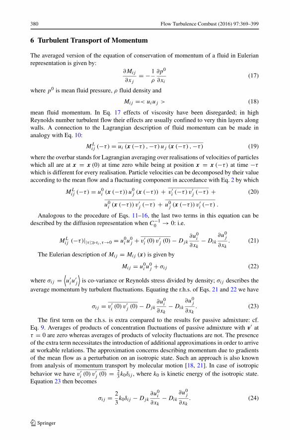
Fig. 1 Longitudinal stress versus wall-normal distance where⟨u′1u
′1
⟩is variance in longitudinal direction
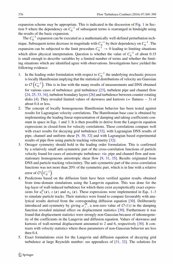
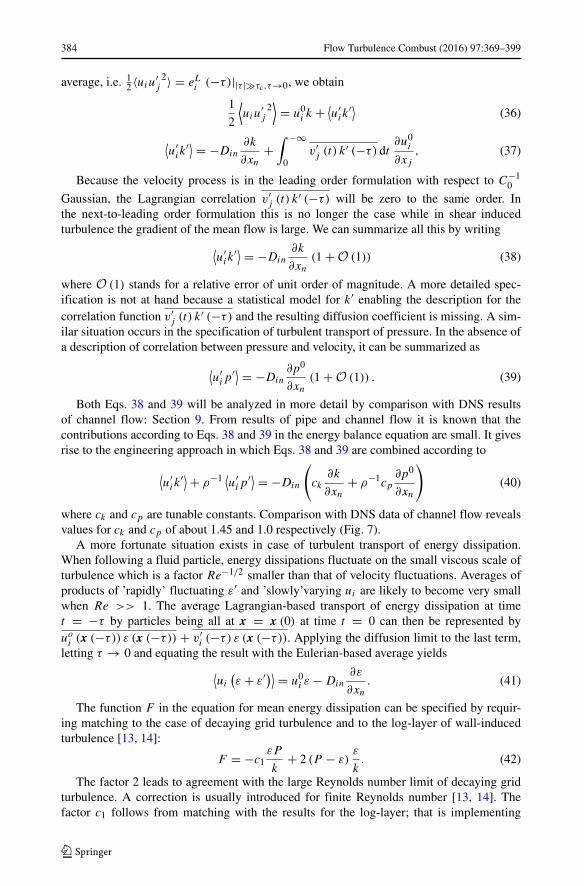
according to DNS, σ11,1 term, σ11,2 terms and σ11,3 terms according to Eq. 50a with each term on the r.h.s.evaluated with the DNS data, and σ11basic according to Eq. 48a with the r.h.s. evaluated with the DNS data
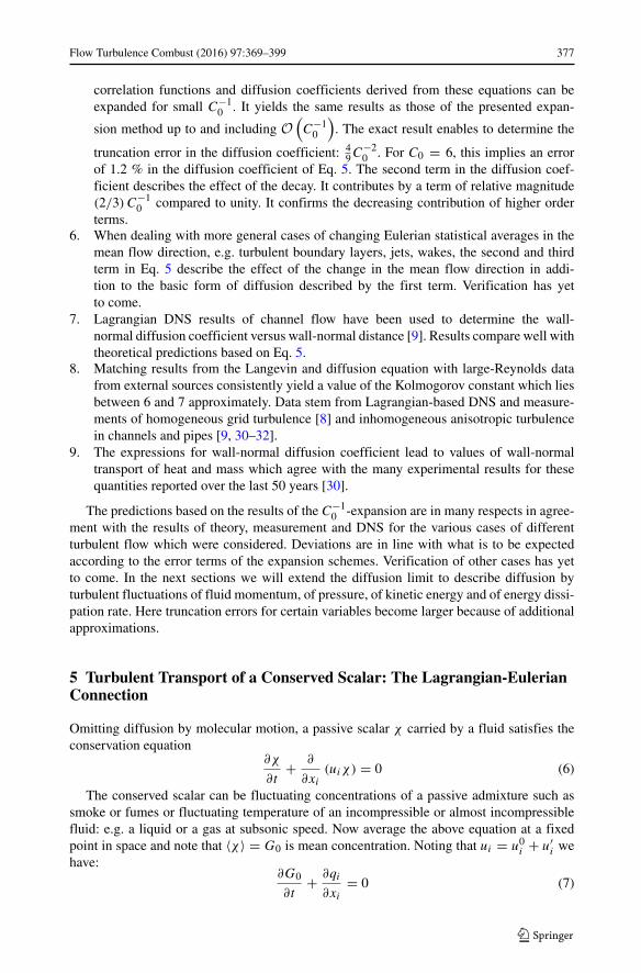
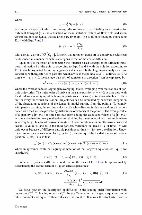
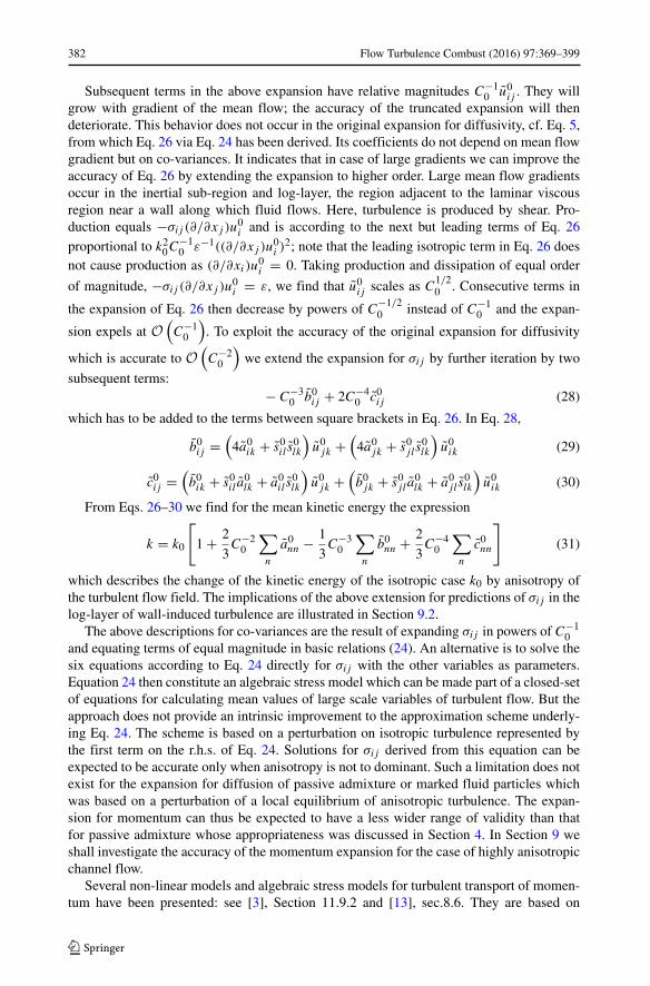
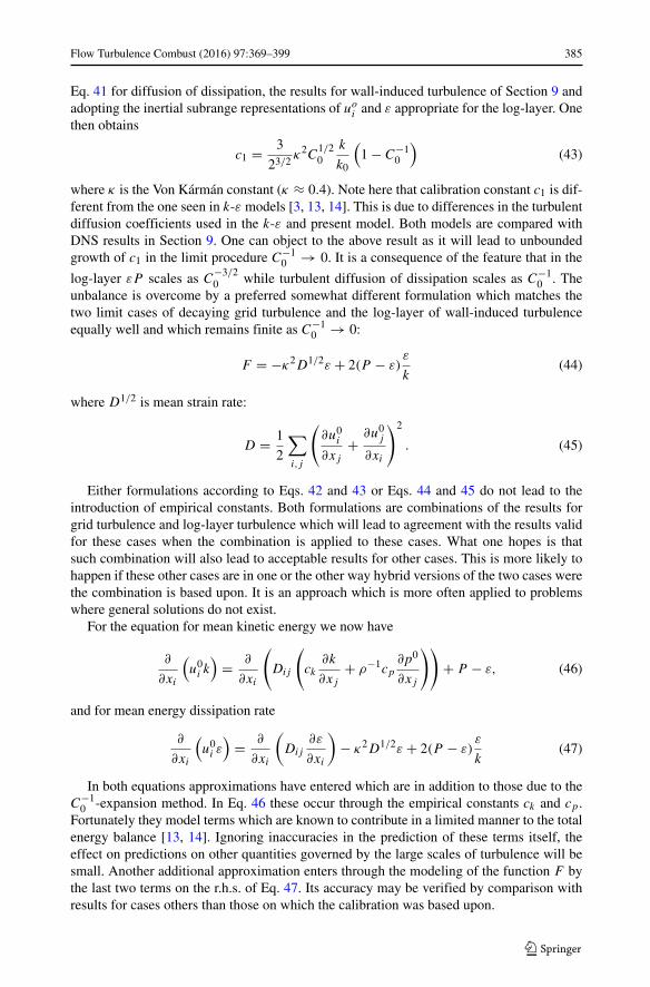
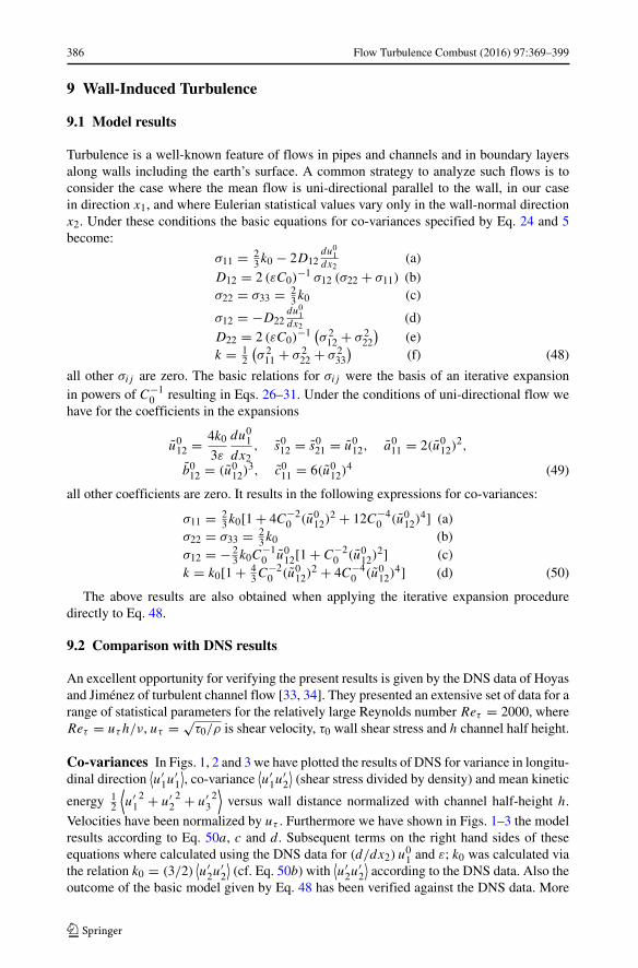
specifically, the results for σ11, σ21 and k according to Eq. 48 using the DNS data to calcu-late the right hand sides have been presented in Figs. 1–3. In all cases we took C0 = 6.2,a value which is in line with previous claims for the value of C0 and which leads to bestoverall agreement.
It is seen that in case of shear stress (Fig. 2) and kinetic energy (Fig. 3) there is goodagreement between the results of DNS and the predictions of the basic model. The agree-ment is somewhat less in case of the longitudinal stress (Fig. 1). It is also seen that theone, two and three term representations according to Eq. 50 tend to come closer to thebasic and DNS results. But the convergence is rather slow indicating that the expansion isat its limit of validity due to large mean-flow-gradient. This may be ascribed to the partic-ular situation in the log-layer. Inserting the asymptotic expressions for u0i and ε valid forthis region and using the leading order scaling for σ12 according to Eq. 50c one finds that
the coefficients in the expansions according to Eqs. 50a − d change from C−20
(u012
)2to
2C−10
(1 − 2C−1
0
). The coefficients in the expansion thus reduce from quadratic to single
powers in C−10 implying slower convergence. The unique position of C−1
0 as scaling param-eter, however, is retained. We also note that according to Eq. 50b, stresses in wall-normaland spanwise directions are equal. On the other hand, the DNS results reveal values forstandard deviations of spanwise velocities which are 15 % larger than those of wall-normalvelocities [33]. Anisotropy in spanwise direction is apparently not captured by the model.This in contrast to the much larger anisotropy seen in longitudinal direction (Fig. 1) and theoverall effect of anisotropy seen in the kinetic energy (Fig. 3): these are reasonably wellpredicted by the basic model. Underprediction of spanwise fluctuations is compensated byover prediction of longitudinal fluctuations, resulting in agreement of kinetic energy for the
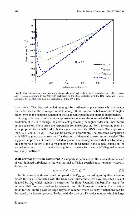
388 Flow Turbulence Combust (2016) 97:369–399
0 0.2 0.4 0.6 0.8 1−1
−0.9
−0.8
−0.7
−0.6
−0.5
−0.4
−0.3
−0.2
−0.1
0
wall−normal distance / h
shea
r st
ress
/ ( ρ
u τ2 )
C0 = 6.2
< u’1u’
2 >
σ12 1term
σ12 2terms
σ12 basic
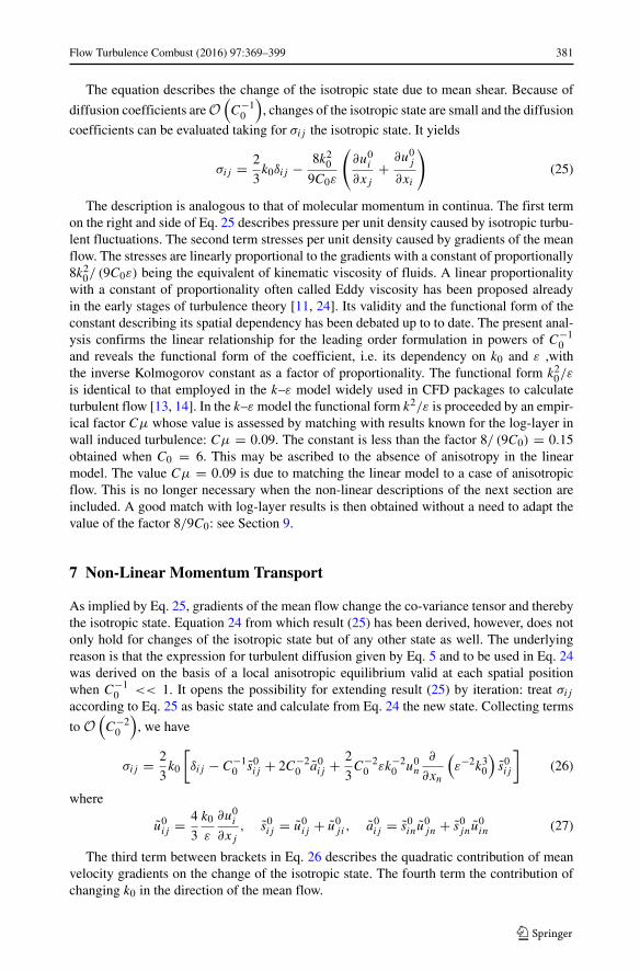
Fig. 2 Shear stress versus wall-normal distance where⟨u′1u
′2
⟩is shear stress according to DNS, σ12,1 term
and σ12,2 terms according to Eq. 50c with each term on the r.h.s. evaluated with the DNS data, and σ12basic
according to Eq. 48d with the r.h.s. evaluated with the DNS data
basic model. The observed deviations might be attributed to phenomena which have notbeen addressed in the developed model: among others, non-linear behavior due to higherorder terms in the damping function of the Langevin equation and internal intermittency.
A pragmatic way to repair in an approximate manner the observed deficiency in theprediction of σ11 is to enlarge the coefficients preceding the higher order non-linear termsin the expansion. These terms are responsible for anisotropy: cf. (50a). Increasing them byan appropriate factor will lead to better agreement with the DNS results. The expressionfor k = (1/2) (σ11 + σ22 + σ33) can be corrected accordingly. The presented comparisonwith DNS suggests that corrections for shear or off-diagonal stresses are not needed. Thesuggested improvement can be extended to general non-homogeneous turbulence by addingthe appropriate factors to the corresponding non-linear terms in the general expansion fornormal stresses σij , i = j , while leaving the expansions for shear or off-diagonal stressesσij , i �= j unaffected.
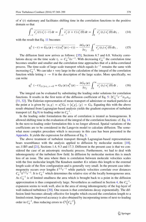
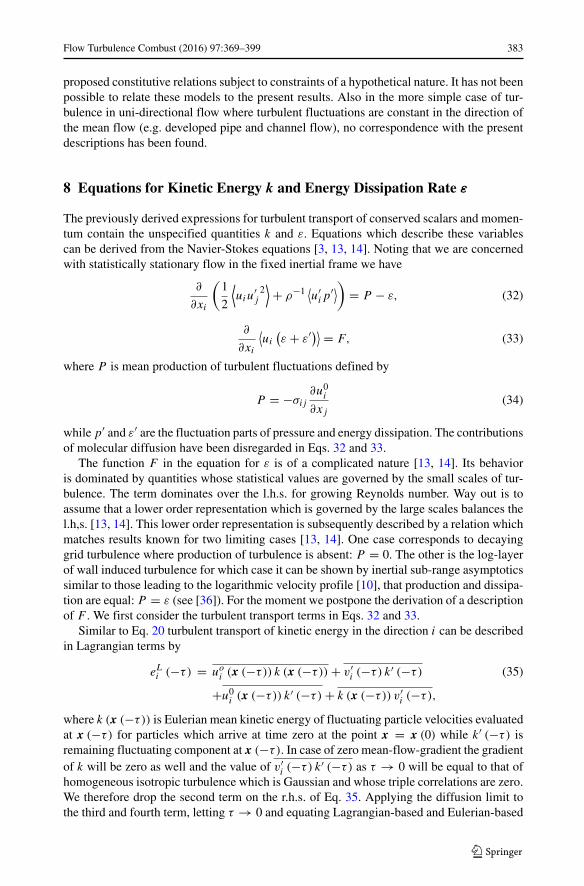
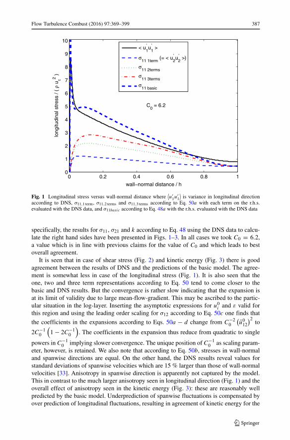
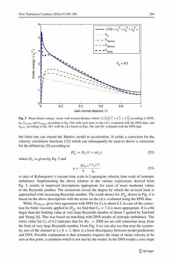
Wall-normal diffusion coefficient An important parameter in the momentum balanceof wall-induced turbulence is the wall-normal diffusion coefficient or turbulent viscositydefined as
νt = −⟨u′1u
′2
⟩/ (∂/∂x2) u01. (51)
In Fig. 4 we have shown νt and compared with D22basic according to Eq. 48e, where asbefore the r.h.s. is evaluated with the DNS data. Furthermore, we have presented a resultdenoted by Dc
22 which includes a correction for finite Reynolds number. The results forturbulent diffusion presented so far originate from the Langevin equation. The equationholds for the limiting case of large Reynolds number where velocity fluctuations can bedescribed by a Markov process. To deal with the case of a Reynolds number which is large
Flow Turbulence Combust (2016) 97:369–399 389
0 0.2 0.4 0.6 0.8 10
1
2
3
4
5
6
kine
tic e
nerg
y / (
uτ2 )
wall−normal distance / h
C0 = 6.2
(1/2) < u’ 21
+ u’ 22
+ u’ 23
>
k0
k2terms
k3terms
kbasic
Fig. 3 Mean kinetic energy versus wall-normal distance where (1/2)⟨u′2
1 + u′22 + u′2
3
⟩according to DNS,
k0, k2 terms and k3 terms according to Eq. 50d with each term on the r.h.s. evaluated with the DNS data, andkbasic according to Eq. 48f with the r.h.s.based on Eqs. 48a and 48c evaluated with the DNS data
but finite one can extend the Markov model to acceleration. It yields a correction for thevelocity correlation functions [32] which can subsequently be used to derive a correctionfor the diffusivity [9] according to
Dcij = Dij (1 + ηδij ) (52)
where Dij is given by Eq. 5 and
η = 3C0
4
ε1/2ν1/2
ko
(53)
is ratio of Kolmogorov’s viscous time scale to Lagrangian velocity time scale of isotropicturbulence. Implementing the above relation in the various expressions derived fromEq. 5, results in improved descriptions appropriate for cases of more moderate valuesof the Reynolds number. The extensions reveal the degree by which the inviscid limit isapproached with increasing Reynolds number. The result shown for Dc
22 shown in Fig. 4 isbased on the above descriptions with the terms on the r.h.s. evaluated using the DNS data.
While D22basic gives best agreement with DNS for C0 is about 6.2, in case of the correc-tion for finite viscosity applied in Dc
22, we find that C0 = 7.4 is more appropriate. It is a bitlarger than the limiting value at very large Reynolds number of about 7 quoted by Sawfordand Yeung [8]. This was based on matching with DNS results of isotropic turbulence. Thelower value for C0 of 6.2 indicates that for Reτ = 2000 we are still somewhat away fromthe limit of very large Reynolds number. From Fig. 4 we can also see that near the symme-try axis of the channel at x2/h = 1, there is a local discrepancy between model predictionsand DNS. Possible explanation is that symmetry requires the slope of mean velocity to bezero at this point, a condition which is not met by the model. In the DNS results a zero slope
390 Flow Turbulence Combust (2016) 97:369–399
0 0.2 0.4 0.6 0.8 10
0.02
0.04
0.06
0.08
0.1
0.12
u τ h
)
wall−normal distance /
diffu
sion
coe
ffici
ent /
(
h
D22c (C
0=7.4)
D22basic
(C0=6.2)
νt
νtk ε
Fig. 4 Turbulent diffusion coefficients according to models and DNS eddy viscosity versus wall-normaldistance, where νt turbulent eddy viscosity defined by Eq. 51 with the r.h.s evaluated using the DNS data,D22basic according to Eq. 48e with the terms on the r.h.s. evaluated using the DNS data, Dc
22 according toEqs. 52 and 53 with the r.h.s evaluated using the DNS data, and νkε
t turbulent viscosity of the k − ε modeldefined by Eq. 54 with the r.h.s. evaluated using the DNS data
is accomplished by the action of viscosity which is absent in the model. Furthermore, wehave presented in Fig. 4 the result of the k–ε model where turbulent viscosity is describedaccording to
νkεt = cμk2 / ε (54)
where cμ = 0.09 and the r.h.s. evaluated using the DNS data. This result will be discussedin Section 9.3.
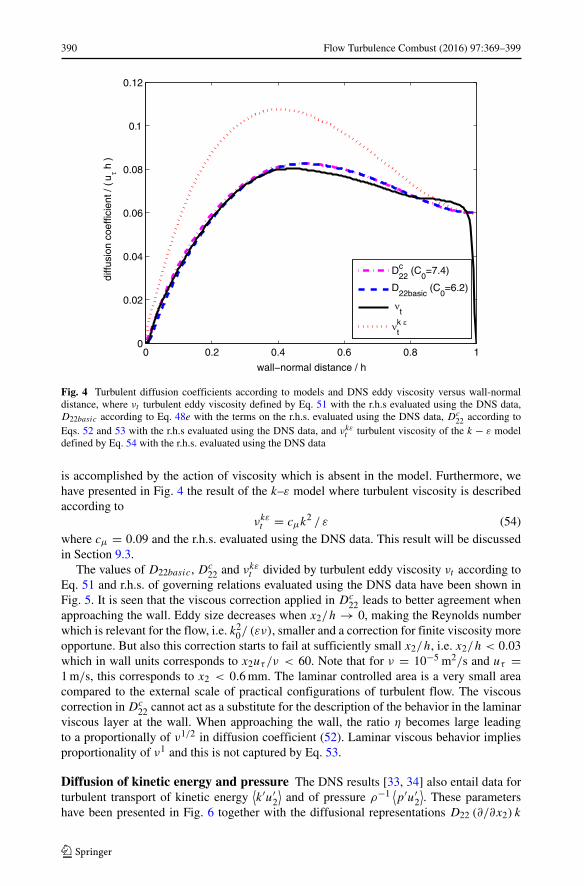
The values of D22basic, Dc22 and νkε
t divided by turbulent eddy viscosity νt according toEq. 51 and r.h.s. of governing relations evaluated using the DNS data have been shown inFig. 5. It is seen that the viscous correction applied in Dc
22 leads to better agreement whenapproaching the wall. Eddy size decreases when x2/h → 0, making the Reynolds numberwhich is relevant for the flow, i.e. k20/ (εν), smaller and a correction for finite viscosity moreopportune. But also this correction starts to fail at sufficiently small x2/h, i.e. x2/h < 0.03which in wall units corresponds to x2uτ /ν < 60. Note that for ν = 10−5 m2/s and uτ =1m/s, this corresponds to x2 < 0.6mm. The laminar controlled area is a very small areacompared to the external scale of practical configurations of turbulent flow. The viscouscorrection in Dc
22 cannot act as a substitute for the description of the behavior in the laminarviscous layer at the wall. When approaching the wall, the ratio η becomes large leadingto a proportionally of ν1/2 in diffusion coefficient (52). Laminar viscous behavior impliesproportionality of ν1 and this is not captured by Eq. 53.
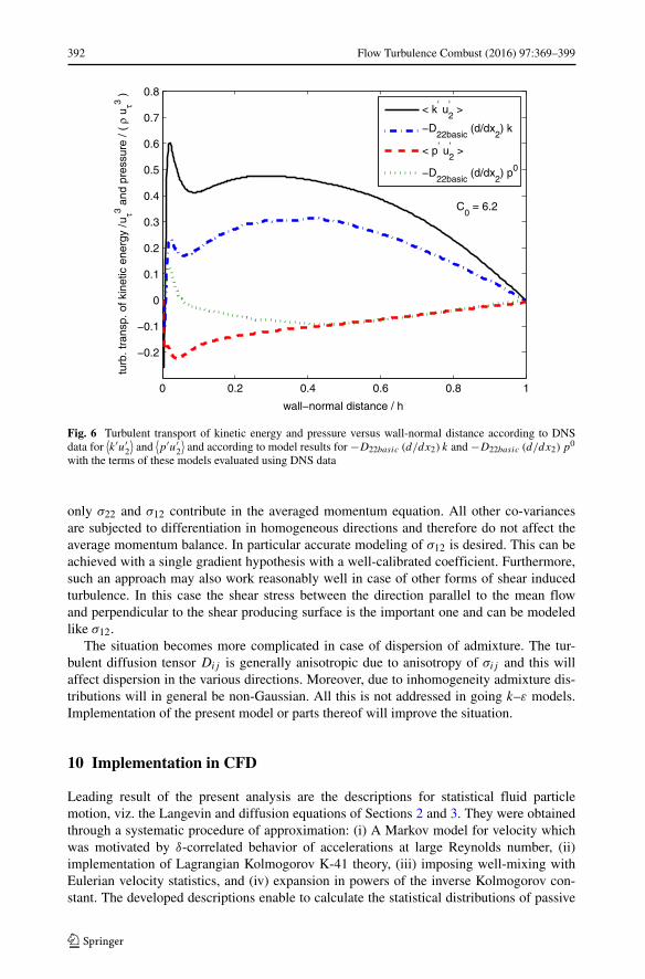
Diffusion of kinetic energy and pressure The DNS results [33, 34] also entail data forturbulent transport of kinetic energy
⟨k′u′
2
⟩and of pressure ρ−1
⟨p′u′
2
⟩. These parameters
have been presented in Fig. 6 together with the diffusional representations D22 (∂/∂x2) k
Flow Turbulence Combust (2016) 97:369–399 391
0 0.2 0.4 0.6 0.8 10
0.5
1
1.5
2
2.5
wall−normal distance /
diffu
sion
coe
ffici
ent /
turb
ulen
t vis
cosi
ty
h
D22c / ν
t (C
0=7.4)
D22basic
/ νt (C
0=6.2)
νtk ε / ν
t
Fig. 5 Diffusion coefficients divided by turbulent viscosity versus wall-normal distance, where all variablesare as defined in Fig. 3
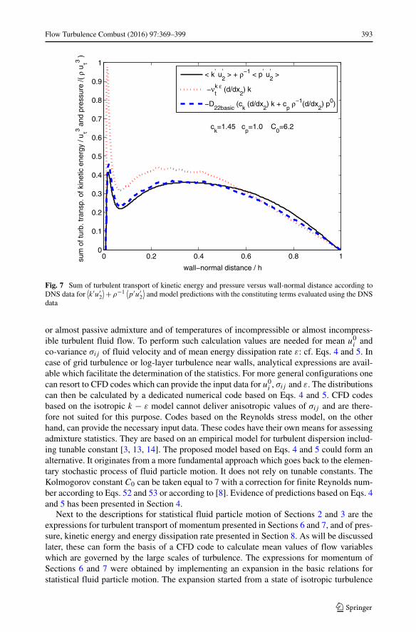
and ρ−1D22(∂/∂x2)p0. The differences are in line with Eqs. 38 and 39 and accompanying
statements. In Fig. 7 we have compared the sum of⟨k′u′
2
⟩and ρ−1
⟨p′u′
2
⟩with the diffusional
representation of Eq. 40 taking ck = 1.45 and cp = 1.0. Furthermore, we have shown thediffusional representation used in the k–ε model [13, 14]:
⟨k′u′
2
⟩ + ρ−1 ⟨p′u′
2
⟩ = −cμ
σk
k2
ε
dk
dx2(55)
with cμ = 0.09 and σk = 1.
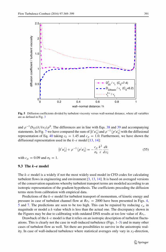
9.3 The k–ε model
The k–ε model is a widely if not the most widely used model in CFD codes for calculatingturbulent flows in engineering and environment [3, 13, 14]. It is based on averaged versionsof the conservation equations whereby turbulent transport terms are modeled according to anisotropic representation of the gradient hypothesis. The coefficients preceding the diffusionterms stem from calibration with empirical data.
Predictions of the k–ε model for turbulent transport of momentum, of kinetic energy andpressure in case of turbulent channel flow at Reτ = 2000 have been presented in Figs. 4,5 and 7. The predictions are seen to be too high. This can be repaired by reducing cμ inmagnitude or model a k-value which is less than the actual one. The discrepancy shown inthe Figures may be due to calibrating with outdated DNS results at too low value of Reτ .
Drawback of the k–ε model is that it relies on an isotropic description of turbulent fluctu-ations. This is clearly not the case in wall-induced turbulence (Figs. 1–3) and in many othercases of turbulent flow as well. Yet there are possibilities to survive in the anisotropic real-ity. In case of wall-induced turbulence where statistical averages only vary in x2-direction,
392 Flow Turbulence Combust (2016) 97:369–399
0 0.2 0.4 0.6 0.8 1
−0.2
−0.1
0
0.1
0.2
0.3
0.4
0.5
0.6
0.7
0.8
wall−normal distance / h
turb
. tra
nsp.
of k
inet
ic e
nerg
y / u
τ3 and
pre
ssur
e / (
ρ u
τ3 )
C0 = 6.2
< k’ u’2 >
−D22basic
(d/dx2) k
< p’ u’2 >
−D22basic
(d/dx2) p0
Fig. 6 Turbulent transport of kinetic energy and pressure versus wall-normal distance according to DNSdata for
⟨k′u′
2
⟩and
⟨p′u′
2
⟩and according to model results for −D22basic (d/dx2) k and −D22basic (d/dx2) p0
with the terms of these models evaluated using DNS data
only σ22 and σ12 contribute in the averaged momentum equation. All other co-variancesare subjected to differentiation in homogeneous directions and therefore do not affect theaverage momentum balance. In particular accurate modeling of σ12 is desired. This can beachieved with a single gradient hypothesis with a well-calibrated coefficient. Furthermore,such an approach may also work reasonably well in case of other forms of shear inducedturbulence. In this case the shear stress between the direction parallel to the mean flowand perpendicular to the shear producing surface is the important one and can be modeledlike σ12.
The situation becomes more complicated in case of dispersion of admixture. The tur-bulent diffusion tensor Dij is generally anisotropic due to anisotropy of σij and this willaffect dispersion in the various directions. Moreover, due to inhomogeneity admixture dis-tributions will in general be non-Gaussian. All this is not addressed in going k–ε models.Implementation of the present model or parts thereof will improve the situation.
10 Implementation in CFD
Leading result of the present analysis are the descriptions for statistical fluid particlemotion, viz. the Langevin and diffusion equations of Sections 2 and 3. They were obtainedthrough a systematic procedure of approximation: (i) A Markov model for velocity whichwas motivated by δ-correlated behavior of accelerations at large Reynolds number, (ii)implementation of Lagrangian Kolmogorov K-41 theory, (iii) imposing well-mixing withEulerian velocity statistics, and (iv) expansion in powers of the inverse Kolmogorov con-stant. The developed descriptions enable to calculate the statistical distributions of passive
Flow Turbulence Combust (2016) 97:369–399 393
0 0.2 0.4 0.6 0.8 10
0.1
0.2
0.3
0.4
0.5
0.6
0.7
0.8
0.9
1
wall−normal distance / h
sum
of t
urb.
tran
sp. o
f kin
etic
ene
rgy
/ uτ3 a
nd p
ress
ure
/( ρ
uτ3 )
ck=1.45 c
p=1.0 C
0=6.2
< k’ u’2 > + ρ−1 < p’ u’
2 >
−νtk ε (d/dx
2) k
−D22basic
(ck (d/dx
2) k + c
pρ−1(d/dx
2) p0)
Fig. 7 Sum of turbulent transport of kinetic energy and pressure versus wall-normal distance according toDNS data for
⟨k′u′
2
⟩+ρ−1⟨p′u′
2
⟩and model predictions with the constituting terms evaluated using the DNS
data
or almost passive admixture and of temperatures of incompressible or almost incompress-ible turbulent fluid flow. To perform such calculation values are needed for mean u0i andco-variance σij of fluid velocity and of mean energy dissipation rate ε: cf. Eqs. 4 and 5. Incase of grid turbulence or log-layer turbulence near walls, analytical expressions are avail-able which facilitate the determination of the statistics. For more general configurations onecan resort to CFD codes which can provide the input data for u0i , σij and ε. The distributionscan then be calculated by a dedicated numerical code based on Eqs. 4 and 5. CFD codesbased on the isotropic k − ε model cannot deliver anisotropic values of σij and are there-fore not suited for this purpose. Codes based on the Reynolds stress model, on the otherhand, can provide the necessary input data. These codes have their own means for assessingadmixture statistics. They are based on an empirical model for turbulent dispersion includ-ing tunable constant [3, 13, 14]. The proposed model based on Eqs. 4 and 5 could form analternative. It originates from a more fundamental approach which goes back to the elemen-tary stochastic process of fluid particle motion. It does not rely on tunable constants. TheKolmogorov constant C0 can be taken equal to 7 with a correction for finite Reynolds num-ber according to Eqs. 52 and 53 or according to [8]. Evidence of predictions based on Eqs. 4and 5 has been presented in Section 4.
Next to the descriptions for statistical fluid particle motion of Sections 2 and 3 are theexpressions for turbulent transport of momentum presented in Sections 6 and 7, and of pres-sure, kinetic energy and energy dissipation rate presented in Section 8. As will be discussedlater, these can form the basis of a CFD code to calculate mean values of flow variableswhich are governed by the large scales of turbulence. The expressions for momentum ofSections 6 and 7 were obtained by implementing an expansion in the basic relations forstatistical fluid particle motion. The expansion started from a state of isotropic turbulence
394 Flow Turbulence Combust (2016) 97:369–399
(Section 6). In this way the statistical structure of the k − ε model was recovered. Different,however, was the coefficient of turbulent diffusion which no longer resorted to a tunableconstant but was defined by the Kolmogorov constant. Descriptions for anisotropy resultedfrom the higher order terms of the expansion. Comparing the results with DNS results ofchannel flow at Reτ =2000 [33, 34] revealed some interesting results (Section 9). Despitestrong anisotropy and inhomogeneity, values of shear stress (Fig. 2), kinetic energy (Fig. 3)and wall-normal diffusion (Figs. 4 and 5) were predicted in a satisfactory manner at all wallnormal distances except from the narrow viscous controlled areas near the boundaries. Thelarge longitudinal stress was less well predicted (Fig. 1) and differences between statisticalvalues of span-wise and wall-normal fluctuations were absent altogether. Apparently higherorder terms in the expansion no longer fully address the features of anisotropy in parts of thestress tensor when anisotropy is very large. A numerical code based on the presented equa-tions could partly repair such inaccuracy by applying correction factors in front of the higherorder terms of the expansion for normal stress in mean flow direction. The fundamentallybased core of the model remains intact.
The presented equations for mean momentum and co-variances contain as unknownsmean kinetic energy k and mean energy dissipation rate ε. Equations which specify thesevariables can be formulated in a manner similar to the procedures underlying the conven-tional k − ε model equations [3, 13, 14]. Different in the present case is that expressionsfor turbulent transport in these equations can be deduced from the more fundamentallybased relations for statistical fluid particle motion. In case of transport of kinetic energy andpressure, however, only an approximate result could be obtained. Adjustable constants hadto be introduced in the formulation of the diffusion terms in the k-equation whose valuescould be calibrated by matching DNS results of channel flow (Figs. 6 and 7). The deriva-tion of an asymptotically exact result for the diffusion terms was hindered by the absenceof a stochastic model for fluctuations of kinetic energy and pressure. Fortunately contribu-tions of these terms in the k-equation are limited causing limited inaccuracy because of theapproximations.
The equation for mean energy dissipation rate contains production and dissipation termswhich originate from turbulent motions occurring at the small viscous scales. In currentCFD codes these terms are modeled in a semi-empirical manner. The present analysisdoes not provide an alternative. An improvement could come from the diffusion term inthe ε-equation. In the presented ε-equation it has been described in accordance with thefundamentally based relations for statistical fluid particle motion.
Using the presented relations it is possible to formulate a closed system of equationswhich can form the basis of a CFD code. The code enables determination of the Eulerian-based statistical parameters which are governed by the large scales in incompressible oralmost incompressible turbulent flow: mean velocity, anisotropic co-variances, mean pres-sure, mean kinetic energy and mean energy dissipation rate. Next to the equation preservingcontinuity (∂/∂xi)u
oi = 0, the closed system of equations underlying the code consists of:
– Averaged conservation of momentum specified by Eqs. 17 and 22.– The equations for Reynolds stresses which depend non-linearly on the gradient of the
mean velocity, cf. Eqs. 26–31, possibly corrected for effects of large anisotropy onnormal stress in longitudinal direction.
– The equations for k and ε, cf. Eqs. 46 and 47.
In total 13 equations for the variables u0i , p0, σij , k, k0 and ε.The calculated values of u0i , σij , and ε can be used to determine the distributions of
passive or almost passive admixture and of temperatures in turbulent flow at low Mach
Flow Turbulence Combust (2016) 97:369–399 395
number using Eqs. 4 and 5. Boundary conditions can be formulated analogous to thosein conventional CFD models [3, 13, 14]. The closed system of equations is of a similarstructure as that of the CFD code of the k − ε model. The numerical code can be relativelyeasily accomplished by adapting and modifying an existing k − ε based code.
Acknowledgment H.S.Janssen, R.J. van Benthum and H.P. van Kemenade are acknowledged for workingout the DNS data of Hoyas and Jimenez to generate the results of Figs. 1–7.
Open Access This article is distributed under the terms of the Creative Commons Attribution 4.0 Inter-national License (http://creativecommons.org/licenses/by/4.0/), which permits unrestricted use, distribution,and reproduction in any medium, provided you give appropriate credit to the original author(s) and the source,provide a link to the Creative Commons license, and indicate if changes were made.
Appendix: Derivation of the Turbulent Diffusion Modelfrom Lagrangian-Based Statistical Descriptions Using C−1
0 -Expansions
1. Starting point is the Langevin model for Lagrangian-based statistical velocity devel-oped previously [31, 32]. The model is centered around fluctuating particle velocityrelative to mean velocity: cf. Eqs. 1–3. In line with this representation we describe dis-placement of a fluid particle by the sum of a non-random component due to mean flowand a component representing zero-mean random displacement (see also Ref. [17] andRef. [19], Section XVI.5):
xi(t) = xti0 + x′
i (t) (56)
where xti0 is particle track according to Eulerian mean velocity:
dxti0
dt= u0i (x
t0) , xt
i0 = xi0 at t = 0 (57)
where x = x0 is particle position at t = 0.2. For general inhomogeneous turbulent flow the Eulerian-based coefficients in the
Langevin model will vary in magnitude with space coordinate. It makes the coefficientstime-dependent in the Lagrangian-based description of the Langevin model. Repre-senting displacement by Eq. 56 the time dependency occurs in two ways: (i) throughspatial variations when following the particle according to the mean velocity xt
0, and(ii) through dependency on random displacement x′:
λij = λij
(xt0 + x′) , ε = ε
(xt0 + x′) , σij = σij
(xt0 + x′) , (58)
u0i = u0i(xt0 + x′) , a′H
i = a′Hi
(v′, xt
0 + x′)
In the next analysis we shall disregard the dependency on x′. Furthermore we dis-regard the non-linear third term in the damping function as well as a′H
i . We shallshow under point 5,6 and 7 that all these terms yield contributions of relative magni-tude O(C−2
0 ) in the diffusion model. Specification to this order is beyond the scopeof this analysis. The Langevin model which specifies diffusion to leading order andnext-to-leading order now follows from Eqs. 1 and 3 as
dv′i
dt=
(
−1
2C0λij
(xt0
)ε(xt0
) + 1
2λjm
(xt0
)u0k
(xt0
) ∂σmi
(xt0
)
∂xtk0
)
v′j (59)
+ (C0ε
(xt0
))1/2wi (t)
396 Flow Turbulence Combust (2016) 97:369–399
From Eqs. 2, 56 and 57 we obtain
v′i = dx′
i
dt(60)
3. Fluctuating equations (59) and (60) can be transformed into a Fokker-Planck equationfor the joint probability of v′ and x′. The solution is a multi-dimensional Gaussiandistribution with time-dependent parameters: [19], sec.VIII.6. The probability densityfor particle position x′ is specified by the diffusion equation
∂p(x′, t ′
)
∂t ′= ∂
∂x′i
(
x′kv
′i
∂p(x′, t ′
)
∂x′k
)
(61)
subject to a suitably chosen initial distribution at t ′ = 0, i.e. the delta pulse δ(x′) in
case of passive marking of particles at t ′ = 0 and x ′ = 0. Note that the time derivativein the above Eulerian description applies to the coordinate system which moves withthe mean velocity according to Eqs. 56 and 57. To evaluate the diffusion coefficientx′kv
′i we note that
d
dtx′kv
′i = v′
kv′i + x′
k
dv′i
dt= σki(x
t0) + x′
k
dv′i
dt(62)
where the latter term can be calculated by multiplying Eq. 59 with x′k and averaging
x′k
dv′i
dt= −1
2C0λij (x
t0)ε(x
t0)x
′kv
′j + 1
2λjm(xt
0)u0n(x
t0)
∂σmi(xt0)
∂xtn0
x′kv
′j (63)
There is no contribution of the last term of Langevin equation (59) because wi(t)
is only correlated with vi(t). Substituting Eq. 63 into the r.h.s of Eq. 62 results in thefollowing first order differential equation for the diffusion coefficient
d
dt
(xkv
′i
)+ 1
2C0 λij (x
t0) ε(xt
0)x′kv
′j = (64)
σki(xt0) + 1
2λjm(xt
0)u0n(x
t0)
∂σmi(xt0)
∂xtn0
x′kv
′j
subject to the initial condition x′kv
′i = 0 at t ′ = 0. The equation describes the transient
of the diffusion coefficient towards its value valid in the diffusion limit when t τc.This limit value can be time-dependent on the time-scale t τc and can be obtainedby iteration using C−1
0 as small parameter. The leading order follows from a balancebetween the second term on the l.h.s. and the first term on the r.h.s. Substituting thissolution into the neglected other terms and noting that according to our definitionsx′kv
′i = Dki when t τc we obtain in terms of the coordinates of the non-moving
frame
Dkn = 2C−10 ε−1σkiσin + 2C−2
0 ε−2σinσkmu0l∂σmi
∂xl
(65)
− 4C−20 ε−1σinu
0l
∂
∂xl
(ε−1σkmσmi
)
Comparison with previous results [31, 32] reveals an extra contribution of next-to-leading order. It is due to presumed change of the leading order value of the diffusioncoefficient in the direction of the mean flow. Such change was in previous analysisdisregarded: [31], Eq. (44) and subsequent statements.
Flow Turbulence Combust (2016) 97:369–399 397
4. Equation 10 describes how the Eulerian-based representation of transport of fluid par-ticles at the fixed point x can be related to a Lagrangian-based expression involvingparticles moving through this point. We shall here repeat this analysis in a more concisemanner while making use of the moving coordinate system of Eqs. 56 and 57. For theLagrangian-based average of passive admixture transport at time t = −τ we have
qLi (−τ) = G0 (x (−τ)) v′
i (−τ) (66)
where x (−τ) is position of particles at time t = −τ and v′i (−τ) their velocities. For
small values of τ and x′ (−τ) we can approximate the Lagrangian average by using aTaylor expansion:
qLi (−τ) = ∂G0
∂xj0x′j (−τ) v′
i (−τ) . (67)
Applying the diffusion limit, |τ | τc, and letting τ → 0, the Lagrangian averagebecomes equal to the r.h.s. of Eq. 65 except that we have to add a minus sign to cor-rect for the negative sign which appears in the Langevin equation when applied in thenegative time-domain. The Eulerian-based description of average turbulent transport ofadmixture whose concentration reads as χ = 〈χ〉 + χ ′, 〈χ〉 = G0 is given by
⟨χ ′u′
i
⟩.
Setting this description equal to the result derived above, having applied the diffusionlimit yields the gradient expression for admixture transport of Eq. 9.
5. The above results for diffusion were obtained by adopting a number of approximations.This includes disregarding the changes in the coefficients of the Langevin equation dueto random displacement x′: cf. Eq. 59. Its effect can be assessed by Taylor expansionaround x′ = 0. For example: ε(xt
0 + x′) = ε(xt0) + x′
j [(∂/∂xj )ε(x)]x ′=0 + ...., where
x′j = ∫ t
0v′kdt . Here t scales as C−1
0 t∗, t∗ = O (1), in accordance with the correlationtime of fluid particle velocity. Displacements due to random motion are thus small andO(C−1
0 ) during times of correlation. It implies that the second term of the Taylor expan-sion yields a contribution in the leading order term of the damping function which isnext-to-leading order. But this contribution no longer counts when applying averagingto the Langevin equation according to Eq. 63 leading to the specification of the diffu-sion coefficient. The contribution vanishes because it becomes a triple correlation ofzero-mean velocities and displacements. It is zero to first order as velocities and dis-placements are Gaussian to first order. Summarizing, we can replace σie(x
t0) and ε(xt
0)
by σie(xt0+x′) and ε(xt
0+x′)without affecting the accuracy of the two-term expansion.6. Another approximation concerned the neglect of the non-linear third term of the damp-
ing function in Eq. 3. The term is next-to-leading order in the expansion scheme.Implementing this non-linear term in the procedure leading to Eq. 63 leads to meanvalues and triple correlations involving x′ and v′ which are zero because of zero-meanGaussian distributions of x′ and v′. The same happens with the third order term in theTaylor expansion which was disregarded in Eq. 67. Also this term vanishes for zero-mean Gaussian distribution of x′ and v′ making Eq. 67 accurate up to a truncation errorofO(C−2
0 ).7. The fourth term on the r.h.s of Eq. 3 represents the contribution due to non-uniqueness.
As this term is next-leading order we can evaluate its contribution in the diffusion coef-ficient taking the leading order statistical formulations for x′ and v′. To leading orderthe Langevin equation can be expressed as
dv′i
dt= −1
2C0λij0ε0v
′i + (C0ε0)
1/2 wi (t) (68)
398 Flow Turbulence Combust (2016) 97:369–399
where ε0 = ε(x0) and λij0 = λij (x0). Multiply l.h.s and r.h.s. with a′k0
H(v′
0) where
a′k0
H(v′
0) = a′Hk (v′
0, x0) and v′0 = v′(t = 0). Averaging both sides yields
d
dt
(a′k0
H(v′
0)v′i (t)
)= −1
2C0λij0ε0 a′
k0H
(v′0)v
′j (t) (69)
= −1
2C0λij0ε0
d
dt
(a′k0
H(v′
0)x′j (t)
)
= −1
2C0λij0ε0
d
dt
(a′k0
H(v′(τ ))x′
j (t + τ))
Integrating with respect to time from t = −τ to t = 0 where τ |τc| so thatcorrelations have vanished we have
a′k0
Hv′i = 1
2C0λij0ε0 a′
k0H
x′j (70)
Note that we used the property that a′k0
Hv′i = a′
k0H
(t)v′i (t) and a′
k0H
x′j =
a′k0
H(t)x′
j (t) constitute stationary processes whose statistical values do not vary withtime. Eq. 70 can be converted to
a′k0
Hx′n = 2C−1
0 ε−10 σin0 a′
k0H
v′i (71)
where σin0 = σin(x0). Taking a′k0
H = v′k this relation reduces to the leading order
formulation of the diffusion coefficient. Incorporating the above term into the r.h.s. ofEq. 63 or 64 will lead to an extra term on the r.h.s. of diffusion coefficient (65) whichis given by
4C−20 ε−2
0 σki0σml0 a′i0
Hv′m0 (72)
For general forms of a′iH the term will be next-leading order. However, a special sit-
uation arises when a′iH satisfies the well-mixed condition, as should be. It can then be
shown that the above term becomes an anti-symmetric tensor. Its inclusion in the diffu-sion equation results in a convective term only. Its relative magnitude is then O(C−2
0 ):see [31], Eq. (52) and accompanying statements, and [32], Eq. (58) and accompany-ing statements. The contribution of the non-unique term in the Langevin equation todiffusion is thus limited to one of relative magnitude O(C−2
0 ).
8. Outcome of the C−10 -expansion is that Gaussianity can only be required to exist in
the leading order formulation. To model non-Gaussianity in the next-to-leading orderformulation a general term in the damping function has to added which captures thecontribution of cumulants of third and higher order of Eulerian velocities [31, 32].Applying an analysis similar to that under 7 above then shows again that such extraterm only yields contributions in the diffusion model which are O(C−2
0 ).
References
1. Monin, A.S., Yaglom, A.M.: Statistical Fluid Mechanics. Dover Publications (2007)2. Lumley, J.L., Yaglom, A.M.: A century of turbulence. Flow Turbul. Combust. 66(3), 241–286 (2001)3. Pope, S.B.: Turbulent Flows. Cambridge University Press (2000)4. Voth, G.A., La Porta, A., Crawford, A.M., Alexander, J., Bodenschatz, E.: Measurements of particle
accelerations in fully developed turbulence. J. Fluid Mech. 469(1), 121–160 (2002)5. Frisch, U.: Turbulence. Cambridge University Press (1998)6. La Porta, A., Voth, G.A., Crawford, A.M., Alexander, J., Bodenschatz, E.: Fluid particle accelerations in
fully developed turbulence. Nature 409, 1017–1019 (2001)
Flow Turbulence Combust (2016) 97:369–399 399
7. Arneodo, A., et al.: Universal intermittent properties of particle trajectories in highly turbulent flows.Phys. Rev. Lett. 100, 254504 (2008)
8. Sawford, B.L., Yeung, P.: Kolmogorov similarity scaling for one-particle lagrangian statistics. Phys.Fluids 23, 091704 (2011)
9. Kuerten, J.G.M., Brouwers, J.J.H.: Lagrangian statistics of turbulent channel flow at Reτ = 950calculated with direct numerical simulation and langevin models. Phys. Fluids 25(10), 105108 (2013)
10. Tennekes, H., Lumley, J.L.: A First Course in Turbulence. MIT Press (1972)11. Schlichting, H. Boundary-Layer Theory, 7th edn. McGraw-Hill (1987)12. Launder, B.E., Spalding, D.B.: Lectures in Mathematical Models of Turbulence. Academic Press (1987)13. Bernard, P.S., Wallace, J.M.: Turbulent Flow, Analysis, Measurement and Prediction. Wiley (2002)14. Hanjalic, K., Launder, B.E.: Modelling Turbulence in Engineering and the Environment: Second-
Moment Routes to Closure. Cambridge University Press (2011)15. Smith, L.M., Woodruff, S.L.: Renormalization-group analysis of turbulence. Annu. Rev. Fluid Mech. 30,
275–310 (1998)16. Thomson, D.J.: Criteria for the selection of stochastic models of particle trajectories in turbulent flows.
J. Fluid Mech. 180(1), 529–556 (1987)17. Brouwers, J.J.H.: On diffusion theory in turbulence. J. Eng. Math. 44(3), 277–295 (2002)18. Reichl, L.E.: A Modern Course in Statistical Physics. Wiley-VCH (2004)19. van Kampen, N.G. Stochastic Processes in Physics and Chemistry, 3rd edn. Elsevier (2007)20. Landau, L.D., Lifshitz, E.M.: Statistical Physics, Part 1. Elsevier, Amsterdam (2007)21. Bird, R.B., Stewart, W.E., Lightfoot, E.N.: Transport Phenomena. Wiley, New York (2007)22. Borgas, M.S.: The multifractal Lagrangian nature of turbulence. Phil. Trans. R. Soc. Lond. A 342(1665),
379–411 (1993)23. Townsend, A.A.: The measurement of double and triple correlation derivatives in isotropic turbulence.
Proc. Camb. Philos. Soc. 43(04), 560 (1947)24. Laufer, J.: The Structure of Turbulence in Fully Developed Pipe Flow. Technical Report 1174, Nat.
Advisory Comm. Aeronaut. (1954)25. Morrison, J.F., McKeon, B.J., Jiang, W., Smits, A.J.: Scaling of the streamwise velocity component in
turbulent pipe flow. J. Fluid Mech. 508, 99–131 (2004)26. Klebanoff, P.S.: Characteristics of Turbulence in a Boundary Layer with Zero Pressure Gradient.
Technical Report 1247, Nat. Advisory Comm. Aeronaut. (1955)27. Taylor, G.I.: Diffusion by continuous movements. Proc. London Math. Soc. s2–20(1), 196–212 (1922)28. Sawford, B.L.: Recent developments in the lagrangian stochastic theory of turbulent dispersion. Bound.-
Layer Meteorol. 62(1–4), 197–215 (1993)29. Wilson, J.D., Sawford, B.L.: Review of Lagrangian stochastic models for trajectories in the turbulent
atmosphere. Bound.-Layer Meteorol. 78(1–2), 191–210 (1996)30. Brouwers, J.J.H.: Langevin equation of a fluid particle in wall-induced turbulence. Theor. and Math.
Phys. 163(2), 677–695 (2010). [open access]31. Brouwers, J.J.H.: Langevin and diffusion equation of turbulent fluid flow. Phys. Fluids 22(8), 085102
(2010). [open access]32. Brouwers, J.J.H.: Statistical description of turbulent dispersion. Phys. Rev. E 86(6), 066309 (2012).
[open access]33. Hoyas, S., Jimenez, J.: Scaling of the velocity fluctuations in turbulent channels up to Reτ = 2003. Phys.
Fluids 18(011702) (2006)34. Hoyas, S., Jimenez, J.: Reynolds number effects on the reynolds-stress budgets in turbulent channels.
Phys. Fluids 20(101511) (2008)35. Stratonovich, R.L.: Topics in the theory of random noise, vol. I. Gordon & Breach, New York (1981)36. Brouwers, J.J.H.: Dissipation equals production in the log layer of wall-induced turbulence. Phys. Fluids
19(10), 101702 (2007)


![Statistical analysis of turbulent pipe flow : a numerical ... · erally accepted phenomena of a turbulent flow (see e.g. [61] or [94]). Other features that have been addressed are](https://img.pdfslide.us/doc/110x75/5fb15129e7cb77378d7f3ce5/statistical-analysis-of-turbulent-pipe-flow-a-numerical-erally-accepted-phenomena.jpg)