Statistical Models of Criminal Behavior:

The Effects of Law Enforcement Actions

Paul A. Jones1, P. Jeffrey Brantingham2 and Lincoln R. Chayes1

September 11, 2009

1Department of Mathematics, UCLA, Los Angeles, CA 90059–1555 USA2Department of Anthropology, UCLA, Los Angeles, CA 90059–1553 USA

Abstract: We extend an agent–based model of crime–pattern formation initiated in Short et al. by

incorporating the effects of law enforcement agents. We investigate the effect that these agents have on

the spatial distribution and overall level of criminal activity in a simulated urban setting. Our focus is

on a two–dimensional lattice model of residential burglaries, where each site (target) is characterized by

a dynamic attractiveness to burglary and where criminal and law enforcement agents are represented

by random walkers. The dynamics of the criminal agents and the target–attractiveness field are, with

certain modifications, as described in Short et al. Here the dynamics of enforcement agents are affected

by the attractiveness field via a biasing of the walk, the detailed rules of which define a deployment strat-

egy. We observe that law enforcement agents, if properly deployed, will in fact reduce the total amount

of crime, but their relative effectiveness depends on the number of agents deployed, the deployment

strategy used, and spatial distribution of criminal activity. For certain policing strategies, continuum

PDE models can be derived from the discrete systems. The continuum models are qualitatively similar

to the discrete systems at large system sizes.

1 Introduction

In a previous work [42] a model of criminal behavior was introduced, the purpose of which was todescribe, at the statistical level, evolving patterns of criminal activity. The essential componentsof the model are (a) itinerant criminal agents and (b) target attractiveness. An important featureof the model is that the attractiveness is dynamically updated in response to the history of activityat the target. This in turn has led – at least within the context of the model – to the successfulprediction of crime hotspots. The purpose of the current work is to introduce and study the effectsof a third (essential) component in the model, namely the presence of law enforcement agents.

We remark that, in the context of this and the earlier work, no serious effort is made to calibratethe model to correspond with actual criminal activities on realistic time scales. This is possible, butis the subject of ongoing research. The goal of these studies is to gain a mechanistic understanding

1

of the observed phenomena. It is our belief that the observed large–scale, long-time events are aconsequence of cooperative behavior among many interacting constituents. Hence, in accord withthe understanding of other cooperative phenomena (e.g., phase transitions in condensed matterphysics), once the essential features have been encapsulated, the correct phenomenology will beexhibited independent of the finer details. It is our hope that with the general understandinggained concerning the nature of crime hotspots and a general ansatz concerning the nature ofpolice/criminal interactions, it will be possible to suggest strategies for the allocation of policeresources to efficiently combat real-world crime.

1.1 Background

It is known that crime is not distributed evenly spatially or temporally. Indeed, even at the locallevel, a burglary at a particular location evidently enhances the prospects of future criminal activityat the same and at nearby locations [1, 25, 26, 27, 28, 42]. One explanation for this effect is found inthe “broken windows” theory [50] which posits that the disorder that results from criminal activity– graffiti, broken doors and windows – increases the future rate of such activities [29]. In particular,it is not unreasonable to suppose that after a successful burglary the criminal or an associate is morelikely to revisit the “easy” target [28, 51]. Moreover, there are mid and long–range correlations:Some neighborhoods are simply “worse” (i.e. enhance and attract criminal activities more) thanothers [6, 7, 10, 23, 38]. However, quite apart from these intrinsic “background” considerations, itappears that the local mechanism has the potential to create hotspots – areas where the burglaryrate is substantially higher than that of its surroundings.

With these considerations in mind, let us proceed with an informal description of the model inShort et al. [42]; a more precise description will be provided in the next subsection. The brokenwindows effect is reflected in a dynamical property of the targets: associated with each target(house) there is a number which represents the “attractiveness” of the location for burglary bycriminal agents. This attractiveness plays two roles: (i) it biases movement of the agents towardtargets of higher attractiveness and (ii) determines the rate at which (or probability that) a target isburglarized given that a criminal agent is at the target location. Moreover, the value itself representsthe sum of two terms. One component is static and is derived from the intrinsic properties of thehouse and its neighborhood [2, 12, 21, 35, 39, 40]. The other component is dynamic and is relatedto local burglary events. How the dynamical component evolves in time will be described shortly.

Thus, effectively, a criminal agent at a particular location has a choice: The agent can eithercommit a burglary, the probability of which increases with the attractiveness value, or the agent“chooses” to move to a neighboring house. If burglary has been chosen, then the agent is removedfrom the model. This represents the criminal returning home with the illicit acquisitions. On theother hand, if the criminal agent chooses to move, a neighboring location is selected with a biasfavoring neighbors with greater attractiveness.

Next, let us briefly discuss how criminals enter and leave the system. As mentioned above, aftera criminal agent has committed a burglary the agent is removed from the system. Criminals can

2

also be randomly removed from the system. Indeed since most (low profile) house burglaries arecommitted by criminal agents who live relatively close to their target [11, 39, 5, 6, 43], it seemsreasonable to incorporate a mechanism that limits how far criminals wander from their startingpoint. To this end, a rate of removal from the system is introduced which may, in the abovevernacular, be regarded as a third choice: With some relatively low probability, the agent is simplyremoved from the environment without having committed a burglary. This probability representshow long, on average, a criminal agent is willing to wander before giving up and returning home.Finally, to model the agents starting from their homes and commencing their searches for a suitabletarget, criminals are introduced at each site with a given rate.

It is evident that the behavior of criminal agents is strongly tied to the attractiveness valuesin their local environments. The key feature of the model is a feedback mechanism whereby theconverse is also true: local attractiveness values are increased by criminal activities. Specifically, inthe event that a house is burglarized, the dynamic attractiveness of the targeted house is increasedby a fixed amount [27, 28]. 1 This does not represent a permanent change, nor is this the onlymechanism for increase of attractiveness. First, the dynamic attractiveness of each house decaysin time; thus, if not subjected to further criminal activity, the total attractiveness value of a targetreturns to its baseline value. Second, the dynamic attractiveness is spatially diffusive: local valuesare adjusted in accord with the average among neighboring houses.

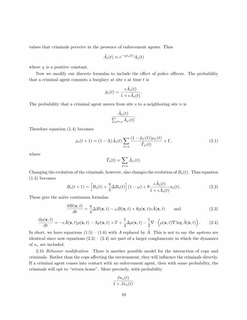
In the present work, police agents will be introduced into the above model; a schematic overviewof the entire setup is provided in Figure 1. Police agents will be permitted to explore the urbanenvironment according to various strategies (for general background see [34, 37, 48]) the centralpurpose of this work is to investigate different strategies in order to ascertain their relative effec-tiveness at reducing criminal activity. To accomplish this, we must first decide how to model theinteraction of police agents with the criminal agents and/or the urban environment. The vast ma-jority of burglaries go unsolved [52] and, in any case, on-the-spot arrests of burglars are rare. Thusno attempt will be made to model apprehension of criminals by law enforcement agents. Instead,we will aim to incorporate the deterrent effect of police into the system.

Deterrent effects will be modeled in two ways, the first of which impacts criminals directlyand the second via a short-term effect of police agents on the urban environment. In general, onthe basis of obvious considerations, criminals will avoid committing crimes in the presence of lawenforcement. See discussion in [17]. Thus one reasonable mode of interaction is that on encounterwith a police agent, a criminal agent might – prematurely – decide to return home. The secondmode alters the environment: proximity of police will tend to make the local environment lessattractive to the criminal elements. Hence by reducing the attractiveness value in accord with the

1It is important to note that, in the context of the model, not all criminal actions need be interpreted as actual

burglary events. Thus the so called “burglary events” – standing notation to which we will adhere – can represent

any criminal activity that increases the perceived attractiveness of the target. Crimes, such as attempted burglaries

and vandalism, that are committed on a property may indeed raise that house’s attractiveness to criminal elements.

Further, see other low level criminal activities done in the neighboring environment, such as a hole cut in a fence to

facilitate a getaway, will also increase the rate of future burglaries [29].

3

presence of police agents there will be a diminished rate of criminal activity and a tendency forcriminals to move away from regions with a high concentration of police agents. It is remarkedthat both modes are enforcing the same tendencies. Due to limitations of our own resources, wehave chosen to focus our attentions on the second option.

For each criminal

For each law enforcement agentFor each house

Intial State Return home?

Yes

No

Remove criminal

from simulation

Burgle?

Yes

No

Move criminal

Update BAdd criminals

to simulation

Move law en-

forcement agent

Figure 1: Flowchart summarizing the discrete simulation

1.2 Formulation of the Model

We shall now give a more precise description of the model without police agents. The model can bedefined on any graph G (the geometry of which can closely reflect that of an actual city). Howeverfor simplicity, we shall place the target houses at points on the 2D square lattice Z2. We denotea generic position (site) by s = (i, j) with, e.g. 0 ≤ i ≤ M , 0 ≤ j ≤ N . At each site s, thenumber As(t) represents the attractiveness of the target at s at the integer time t. As noted in theprevious subsection, attractiveness is the sum of two components, As(t) = A0

s +Bs(t), where A0s is

the time-independent component and, Bs(t), evolves dynamically.The evolution in time of Bs(t) is driven by burglary events near s. The probability that a

criminal agent at site s will choose to commit a burglary is

ps(t) =εAs(t)

1 + εAs(t)(1.1)

where ε > 0 determines the effectiveness of As in this context. 2 The increase in the dynamic2The equation (1.1) differs somewhat from its counterpart in [42] since, in that context, the model was driven

by rates rather than probabilities. Although there is a technical distinction between the two approaches, we do not

4

attractiveness at site s that results from Es(t), the number of burglary events at time t, is:

Bs(t+ 1) = Bs(t) + θEs(t)

where θ is the increase in attractiveness from a single burglary.Now the decay of attractiveness over a time step 3 is

Bs(t+ 1) = (1− ω)Bs(t)

where ω, the rate of decay, is a constant between 0 and 1. Finally, the diffusion of attractiveness ismodeled by

Bs(t+ 1) = (1− η)Bs(t) +η

4

∑s′∼s

Bs′(t) (1.2)

where η, the rate of diffusion, is a constant between 0 and 1 and s′ ∼ s denotes s′ is a neighbor ofs – that is ‖s′ − s‖ = 1. Equation (1.2) can be rewritten as

Bs(t+ 1) = Bs(t) +η

4∆Bs(t)

where ∆ is the discrete Laplacian

∆Bs(t) =∑s′∼s

Bs′(t)− 4Bs(t).

Thus, if ns(t) denotes the number of criminal agents at the site s at time t, we may combine all ofthe above to obtain:

Bs(t+ 1) =[Bs(t) +

η

4∆Bs(t)

](1− ω) + θps(t)ns(t). (1.3)

Remark 1. We remark that the equation (1.3) is in actuality a formal identity since, strictlyspeaking, the right hand side is the average value of Bs at time t + 1 given the (random) valuesof the various other quantities at time t. It is not possible to fully justify equation (1.3) by takingthe average of the right side since the random variables ns and ps are not necessarily independent.While, from a mathematical perspective, we consider these points to be important, we do notanticipate a significant impact on the large–scale, long–time behavior of the system to result fromthe neglect of these considerations. This anticipation has been born out by the close similaritiesbetween the discrete agent based models (which, necessarily, includes correlations) and the naıvecontinuum limiting PDE in which these effects have been neglected. Approximations of this sortare not without precedent: In particular, the philosophy, as discussed in Spohn [44], is that theimportant (large–scale) correlations are reflected in the intrinsic non–linearities of the continuum

regard such differences as important. Indeed in the naıve continuum limit, the denominator washes out and thus

coincides with the version of equation (1.1) according to rates.3For present purposes, a single time step is the time scale in which each agent or target is typically updated once.

In the vernacular of spin–systems, this is one Monte Carlo step per spin.

5

limit. In all examples of similar models that have been mathematically analyzed (not to mentiona plethora of systems that have received attention in the physics community), the appropriatecontinuum limit turns out to be essentially that which is obtained by the neglect of local correlations.However, it is not necessarily the case that the continuum parameters are exactly the parametersobtained by the so called naıve scaling. Notwithstanding, in the context of the present work weshall adhere to this ideology and will consider the continuum systems obtained by naive scalingwith neglect of correlations.

In the event that a criminal agent does not commit a burglary, the agent will be removed ormoved to a neighboring site. In the latter case, the site will be chosen randomly, but biased in thedirection of high attractiveness. Here the probability a criminal agent will move from site s to aneighbor r is given by

Ar(t)∑s′∼s

As′(t).

Given the number of criminals, ns(t) at site s, let us now calculate the number that will be atthe site at time t+1. The model, in fact, demands that all of the criminals at site s at time t will begone by time t+1 (criminals agents are allowed one of the following three options: move to anothersite, commit a burglary – in which case they are removed – or be removed without committing aburglary). Thus the expected number of criminals at site s at time t+ 1 is given by the influx fromneighboring sites plus a term accounting for their spontaneous creation:

ρs(t+ 1) = (1− Λ)As(t)∑s′∼s

(1− ps′(t))ρs′(t)Ts′(t)

+ Γ. (1.4)

In the above, Λ is the probability that a criminal will be removed without committing a burglary,Γ is the probability at a criminal will be added the site (representing a new criminal “starting fromhome”) and Ts(t) =

∑s′∼sAs′(t).

This describes the discrete model. In Short et al. [42] the “naıve” continuum limit (c.f. aboveremark) for the above system was derived using a common procedure in mathematical biology[3, 4, 15, 16, 20, 21, 24, 32, 35, 36, 45]:

∂B(x, t)∂t

=η

4∆B(x, t)− ωB(x, t) + θρ(x, t)εA(x, t) (1.5)

∂ρ(x, t)∂t

= −εA(x, t)ρ(x, t)− Λρ(x, t) + Γ +14

∆ρ(x, t)− 12∇ · (ρ(x, t)∇ logA(x, t)) . (1.6)

These resulting equations are closely related to the Keller–Segel model for chemotaxis [13, 14, 19,22, 26, 30, 33, 41, 46, 47].

As the model evolves in time it is noticed that, dependent on parameters and initial conditions,only three distinct types of behaviors of the attractiveness field appear to be possible [42]; outputfrom computer simulations can be found in Figure 2. The simplest is spatial homogeneity (Figure2 i) with an attractiveness field that is essentially the same everywhere. The next possible behavior

6

is dynamic hotspots (not shown). In this regime, hotspots – regions of large value of A and/or highrate of burglary – appear and disappear as time evolves. Hotspots may reappear in the same placesrepeatedly, or they may appear in seemingly random locations. However, it seems that this sortof behavior is a result of random noise augmented by the finite size of the system. In particular,no such behavior is observed in the continuum PDE and in the discrete model, noisy/dynamicbehavior does not persist in large scale systems. This does not imply that the effect is unimportantor irrelevant to actual urban activities. Indeed, it is worth remarking that the latter is moreaccurately modeled by a discrete system than the continuum limit thereof. The third and finalregime is that of stationary hotspots (Figures 2ii–iii). This regime is described by hotspots thatnucleate, grow to a characteristic size, and then remain stationary “for as long as one cares toobserve”; see [18]. Here the system is apparently exhibiting one of many possible long–lived steadystates.

To perform any meaningful analysis on our simulations, we need a metric to determine theamount of criminal activity. Ostensibly, we could use the number of burglary events, but this hasa few drawbacks. First, there are families of systems with the same behavior, but different levels ofcriminal activity for example, the crime patterns in two instances may be the same, but the numberof criminals vary – an effect that can be achieved by reducing θ and increasing Γ. Moreover it ispossible to produce two systems of different sizes with the same crime patterns. Second, burglary isa relativity rare event; the number of burglaries that occur in any given time–step may vary widely.Thus, to draw any meaningful information from the number of burglaries, a temporal average mustbe taken.

The spatial average of Bs(t), which we denote BAv(t), is related to the amount of criminalactivity. For any time, T ,

BAv(T ) = (1− ω)TBAv(0) + θT∑n=1

(1− ω)n−1EAv(T − n+ 1)

where EAv(t) is the spatial average of number of burglaries that occurred at each site at time t.As 0 < ω < 1, BAv(t) provides a reasonable proxy for amount of criminal activity, while averagingout some of the volatility. Thus in what follows, we will we equate BAv(t) to the level of criminalactivity.

This leads to natural question: how much crime do we expect? To answer we exploit therelationship between the discrete and continuum models. Following the procedure used to cal-culate equations (3.4) and (3.5) we estimate the attractiveness and criminal density of spatiallyhomogeneous steady state solutions

B ≡εωA0 + εθΓ− ωΛ +

√(εωA0 + εθΓ− ωΛ)2 + 4εω2A0Λ

2εω−A0 and (1.7)

ρ ≡εωA0 + εθΓ + ωΛ−

√(εωA0 + εθΓ + ωΛ)2 − 4εωΓΛθ

2εΛθ, (1.8)

7

where A0 is the spatial average of A0s. Strictly speaking, these equations are only valid for the

continuum model, but for large enough system sizes the two models behave similarly. Thus, theabove quantities in equations (1.7)–(1.8) provide a reasonable estimate for a steady state solutionwith no hotspots.

When crime hotspots are present, the estimates provided by equations (1.7)–(1.8) are no longervalid. Figure 2 shows that we can expect much higher levels of criminal activity when hotspots arepresent.

2 Law Enforcement

In this section we add law enforcement agents to the above model with the goal of reducing theamount of criminal activity in the system. In the simulations and the linear stability analysispresented by Short et al. [42], it is clear that the presence or absence of hotspots is a thresholdphenomenon – small changes in parameters can create a large change in the system. Furthermore,as demonstrated by simulations of the model used in this present work (Figure 2), the presence ofhotspots may increase the overall level of criminal activity while the total number of active criminalagents may decline. These two points suggest that a relativity small number of law enforcementagents acting appropriately can have a dramatic effect.

The remainder of this section is divided into three parts. First, in modeling law enforcementagents we must consider their effect on the environment and how criminal agents respond to theirpresence. We then present three different methods to determine the agents’ patrol routes. Finally,we examine the effect of the law enforcement agents in computer simulations. We will observe thatthe primary factor in the law enforcement agents’ effectiveness is their deployment strategy.

2.1 Modeling the Effects of Law Enforcement

We add law enforcement agents to the model starting with the lattice version. Let κs(t) be thenumber of enforcement agents at the site s at time t. These agents will only attempt to deter thecriminal agents from committing burglary events. Below, we will present two mechanisms: Thefirst modifies how criminal agents perceive their environments. The other has a direct effect on theagents’ actions.

2.1a Perception modification In the context of the model, both the movement of a criminalagent and the criminal agent’s “decision” to commit a burglary are affected only by the local targetattractiveness values. If we allow enforcement agents to modify the attractiveness values, they willultimately be able to control the level of criminal activity. However, the law enforcement effectmust not be permanent; if there is no longer a law enforcement presence, criminal agents will onceagain find the house attractive to burglary.

With these considerations in mind, we introduce a variable that represents the attractiveness

8

(a) t = 1× 103

ACA = 169

BAv = 0.598

(b) t = 32× 103

ACA = 180

BAv = 0.596

(c) t = 128× 103

ACA = 187

BAv = 0.604

(I) Low Activity. Parameters of the

model insufficient to cause hotspots.

The system is nearly spatially homo-

geneous and in particular is close to

the predicted value:

BAv

`128× 103´

= 0.604

and B = 0.598.

(a) t = 1× 103

ACA = 2310

BAv = 0.525

(b) t = 32× 103

ACA = 1903

BAv = 0.732

(c) t = 128× 103

ACA = 1755

BAv = 0.751

(II) Small Hotspots. Here the spa-

tial average, BAv(128 × 103) =

0.751, is much higher than the

predicted homogeneous equilibrium

value, B = 0.352. So we see that

the formation of hotspots does not

just simply redistribute criminal ac-

tivity, instead it more than doubles

the crime rate.

(a) t = 1× 103

ACA = 2891

BAv = 0.359

(b) t = 32× 103

ACA = 2761

BAv = 0.396

(c) t = 128× 103

ACA = 1772

BAv = 0.728

(III) Large Hotspots. Here again we

note that the spatial average, which

is BAv(128 × 103) = 0.773, is much

higher than the predicted homoge-

neous equilibrium value, B = 0.352.

Due to the scaling of the parame-

ters, hotspots take longer to form in

this simulation.

Figure 2: Simulations showing the formation of hotspots. All simulations were run on a 100×100 grid with background

attractiveness, A0 ≡ A0s = 0.1. We output the results of the simulations as a color map using the predicted average

attractiveness, A, as the midpoint. Values of As(t) that satisfy 0 ≤ As(t) ≤ A are represented with colors ranging

from dark blue to light blue to light yellow. The colors light yellow to orange to dark red represent values of As(t)

between A and 5A. Attractiveness values above 5A are also represented with dark red. Each simulation was started

with initial conditions b10000ρc randomly placed criminals and As(0) = A. In Ia – Ic, the simulation was run with

the parameters η = 0.05, θ = 1.0, ω = 4 × 10−4, ε = 0.02, Γ = 2.5 × 10−4, and Λ = 6.25 × 10−4. In IIa–IIc the

simulation was run with parameters η = 0.05, θ = 1.0, ω = 3× 10−3, ε = 8× 10−3, Γ = 4× 10−3, and Λ = 4× 10−3.

Finally, IIIa–IIIc displays the results of a simulation run with parameters η = 0.05, θ = 1.0, ω = 1.875 × 10−4,

ε = 5× 10−4, Γ = 2.5× 10−4, and Λ = 6.25× 10−4. In all of the above, ACA denotes the number of active criminal

agents.

9

values that criminals perceive in the presence of enforcement agents. Thus

As(t) ≡ e−χκs(t)As(t)

where χ is a positive constant.Now we modify our discrete formulas to include the effect of police officers. The probability

that a criminal agent commits a burglary at site s at time t is

ps(t) =εAs(t)

1 + εAs(t).

The probability that a criminal agent moves from site s to a neighboring site n is

An(t)∑s′∼s As′(t)

.

Therefore equation (1.4) becomes

ρs(t+ 1) = (1− Λ)As(t)∑s′∼s

(1− ps′(t))ρs′(t)Ts′(t)

+ Γ, (2.1)

whereTs(t) =

∑s′∼s

As′(t).

Changing the evolution of the criminals, however, also changes the evolution ofBs(t). Thus equation(1.3) becomes

Bs(t+ 1) =[Bs(t) +

η

4∆Bs(t)

](1− ω) + θ

εAs(t)1 + εAs(t)

ns(t). (2.2)

These give the naıve continuum formulas

∂B(x, t)∂t

=η

4∆B(x, t)− ωB(x, t) + θρ(x, t)εA(x, t) and (2.3)

∂ρ(x, t)∂t

= −εA(x, t)ρ(x, t)− Λρ(x, t) + Γ +14

∆ρ(x, t)− 12∇ ·(ρ(x, t)∇ log A(x, t)

). (2.4)

In short, we have equations (1.5) – (1.6) with A replaced by A. This is not to say the systems areidentical since now equations (2.3) – (2.4) are part of a larger conglomerate in which the dynamicsof κs are included.

2.1b Behavior modification There is another possible model for the interaction of cops andcriminals. Rather than the cops affecting the environment, they will influence the criminals directly.If a criminal agent comes into contact with an enforcement agent, then with some probability, thecriminals will opt to “return home”. More precisely, with probability

Jκs(t)1 + Jκs(t)

,

10

a criminal agent at site s will be removed. Here J is a positive constant. Thus equation (1.4)becomes

ρs(t+ 1) = (1− Λ)As(t)∑s′∼s

11 + Jκs′(t)

(1− ps′(t))ρs′(t)Ts′(t)

+ Γ

and the corresponding continuum equation becomes

∂ρ(x, t)∂t

= (−εA(x, t)− Λ− Jκ(x, t)) ρ(x, t) + Γ +14

∆ρ(x, t)− 12∇ · (ρ(x, t)∇ logA(x, t)) . (2.5)

2.2 Dynamics of Law Enforcement

As eluded to earlier, the above only covers part of the relationship between law enforcement,criminals, and their environment; the choice of the law enforcement agents’ patrol routes will alsoinfluence the evolution of the rest of the system. To proceed, we make a couple of simplifyingassumptions on the behavior of the enforcement agents: First, we will demand that the number ofagents on patrol is constant. This reflects, in part, the reality of the limited resources of the policedepartment. We will also assume that the agents move through the city on the ground (i.e., onfoot, car, or some other vehicle). In other words, law enforcement will move through the system,house to house, like the criminal agents. We will propose various strategies that satisfy the abovecriteria and compare their relative effectiveness.2.2a Random Walkers One possibility is for law enforcement agents to patrol random routes. Herepolice do not focus their attention in any particular place. The hope is that criminal activity willbe reduced, as the criminal agents will never know when an enforcement agent will be near. Thismethod has been tried, without much success, in Kansas City [31]. We model the patrols by havingthe law enforcement agents perform an unbiased simple random walk. Thus, the expected numberof law enforcement agents at site s and at time t+ 1 is

κs(t+ 1) =14

∑s′∼s

κs′(t) = κs(t) +14

∆κs(t).

This leads to the continuum equation

∂κ(x, t)∂t

=14

∆κ(x, t). (2.6)

The random patrol method has an obvious downside: enforcement agents will often be locatedin places where the level of criminal activity is already low. We will now introduce two alternativeschemes in which police will concentrate their attention in areas where their presence will have agreater effect.2.2b Cops on the Dots In this scheme the law enforcement agents move randomly but with a biasin the direction of high attractiveness. We will call this method of policing cops on the dots.

Traditionally, some police departments have marked criminal events with markers or dots ona centrally located map. Police officers are then directed to focus on patrolling the areas denoted

11

by the dots. Similarly, in our model the law enforcement agents will tend to patrol areas withrelatively high attractiveness – areas correlated with a high number of individual burglary events.

As we will see, cops on the dots is effective in reducing criminal activity. In the model, criminalagents tend to move from areas of low attractiveness to places where it is higher. Furthermore,criminal agents are more likely to commit crimes in these areas of higher attractiveness. Cops on thedots enforces the reverse tendency. Law enforcement agents patrol areas with high attractivenesswhich reduces the likelihood that criminal agents will commit crimes in these areas (and, in theperception modification model, biases them toward locations with lower attractiveness – placeswhere they are less likely to commit crime). A criminal agent in this situation is more likely toreturn home without having performed any criminal activity. The overall effect is that the globalstatistical rate of burglary is lowered.

We model cops on the dots as follows: The probability a law enforcement agent moves from asite s to a neighboring site d is

Ad(t)∑s′∼sAs′(t)

.

We then see that the expected number of law enforcement agents at site s at time t+ 1 is

As(t)∑s′∼s

κs′(t)Ts′(t)

.

The corresponding continuum equation reads

∂κ(x, t)∂t

=14

∆κ(x, t)− 12∇ · (κ(x, t)∇ logA(x, t)) . (2.7)

2.2c Peripheral Interdiction To maximize the deterrent effect given the constraint of limited re-sources, we introduce another scheme. We will send the law enforcement agents to the perimetersof the hotspots rather than the centers. Since the area of a hotspot grows as a square of its radius,but the perimeter grows only linearly, we expect that this method will be more effective for largerhotspots.

Like cops on the dots, this method reduces criminal activity in areas where the rate is the highest.We have already observed that criminals tend to move to areas with high attractiveness. In fact,this mechanism is largely responsible for the higher rate of criminal activity in these locations.When the law enforcement agents encircle the hotspot they are reducing the rate at which thisadvection occurs, thereby lowering the rate of criminal activity. We call this method of policingperipheral interdiction.

An artifact of the model is a technical difficulty in biasing the enforcement agents towards theperipheries of the hotspots. Of course in realistic situations, this would be achieved by dispatchingunder a centralized control. For our purposes, the steps s→ s′ of the enforcement agents are biasedby weights proportional to exp−|c1Bs′ − c2| where c1 and c2 are constants chosen according tothe parameters of the simulation. This term biases the agents to a certain level of Bs′ ; in ourcase, to a level of attractiveness found on the perimeter of the hotspots. Unfortunately, considering

12

the difficulty of these sorts of biases – not to mention the unrealistic assumption of enforcementagents moving autonomously according to such a bias – a continuum PDE analysis of the peripheralinterdiction strategy is impractical. In this work, we will be content with the results of the discretesimulations.

2.3 Results of Discrete Simulations

In this section we will describe the results of computer simulations of the discrete model outlinedin this work. Here, we only present the output using the perception modification model, but wenote that both schemes are effective in performing the task that they were created for – namelythe reduction of crime.

Regardless of which policing scheme is used we notice some general trends. First, a reductionin criminal activity is correlated with an increase in the number of active criminal agents in oursystem. While surprising at first, this is to be expected. Criminals are removed from the systemwhen they commit a burglary and reintroduced at a rate that is independent of all other quantities.Thus, if there are fewer burglaries there will be more active criminal agents searching for viable tar-gets. Both aspects of the model though simplified, are consistent with criminological observations.The propensity to offend is widely distributed within populations and the suppression of criminalopportunity, though reducing crime, does not eliminate criminal propensity [25].

We also note that even after law enforcement agents have eliminated a hotspot it may be thecase that, nearby, another hotspot will emerge. Indeed, even with law enforcement agents present,a region may be on the verge of instability which means that a hotspot will nucleate with theirdiminished presence. Thus, under certain circumstances, even after hotspots haver been eliminated,we may expect their reappearance – at least temporarily. This effect will be more noticeable withsmall hotspots as they tend to form more quickly while the time it takes the law enforcement agentsto react and respond to a new hotspot does not depend on its size.

The elimination of crime hotspots may have another unfortunate side effect: while crime isreduced in the areas with the highest criminal activity it may actually be increased in areas wherethe criminal activity is lower. Displacement of crime has been one outcome observed in field–basedtests of hotspot policing [9]. If criminal agents are spending more time outside the center of a crimehotspot, they will be more likely to commit crimes in low crime areas.

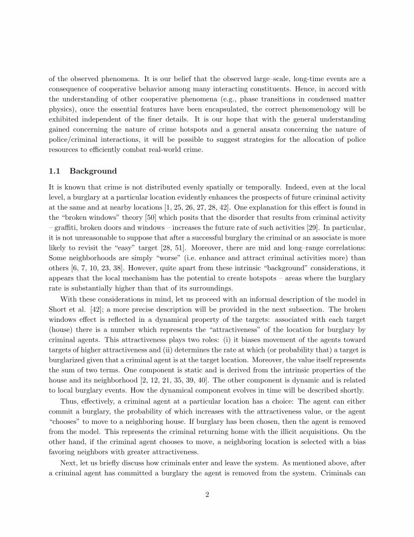
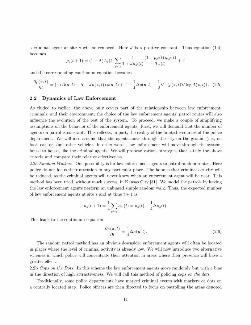
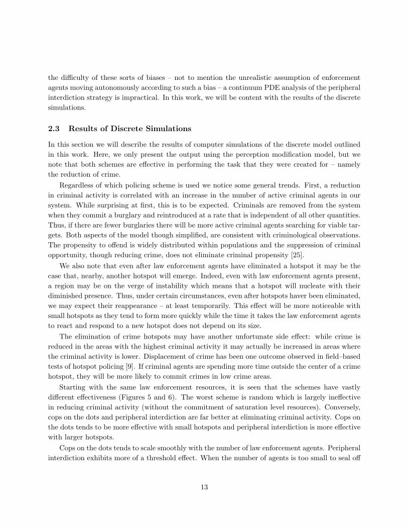
Starting with the same law enforcement resources, it is seen that the schemes have vastlydifferent effectiveness (Figures 5 and 6). The worst scheme is random which is largely ineffectivein reducing criminal activity (without the commitment of saturation level resources). Conversely,cops on the dots and peripheral interdiction are far better at eliminating criminal activity. Cops onthe dots tends to be more effective with small hotspots and peripheral interdiction is more effectivewith larger hotspots.

Cops on the dots tends to scale smoothly with the number of law enforcement agents. Peripheralinterdiction exhibits more of a threshold effect. When the number of agents is too small to seal off

13

the perimeter of even a single hotspot, peripheral interdiction is largely ineffective. However oncethe number of agents has passed a minimum threshold, peripheral interdiction is suddenly effective.This suggests that under extreme conditions of high criminal activity and limited enforcementresources, cops on the dots is the better scheme.

Finally, we see that cops on the dots seems to eliminate hotspots faster than peripheral inter-diction. This is mostly due to the fact that, in the context of the model, there is a delay time forthe biased random movements of the enforcement agents to find a hotspot and set up a perimeter.In practice this would be mitigated by a centralized dispatching scheme: By telling enforcementagents exactly where to patrol, an effective perimeter will be set up almost immediately.

We also notice that the hotspots tend to be eliminated sequentially, when peripheral. Once onehotspot has been eliminated, law enforcement agents are free to move to other hotspots, initiatingaction or helping to seal off their perimeters.

0

0.2

0.4

0.6

0.8

1

0 100 200 300 400 500

BA

v(2

56×

103)

Number of Law Enforcement Agents

RandomCops on the Dots

Peripheral InterdictionEstimated Homogeneous

Figure 3: The relative effectiveness of law enforcement schemes with small hotspots. Each simulation is a continuation

of the one displayed in Figure 2 II – that is, the parameters are the same and initial conditions are given by the state

of the system at Figure 2 IIc (t = 128× 103). The unbiased walkers scheme performs poorly. Peripheral interdiction

and cops on the dots are roughly comparable.

3 Analysis

In this section we will analyze the continuum equations to determine the effect of law enforcementagents. The first step is to simplify equations (2.3) and (2.4). If we assume that A0 is spatially (andtemporally) homogeneous then equation (2.3) can be written in terms of A alone. Furthermore, byvarious rescalings and redefinitions (ρ? = θρ, Γ? = θΓ, η? = 1

4η and C = ωA0 and omitting the ?’s)

14

0

0.2

0.4

0.6

0.8

1

0 100 200 300 400 500

BA

v(2

56×

103)

Number of Law Enforcement Agents

RandomCops on the Dots

Peripheral InterdictionEstimated Homogeneous

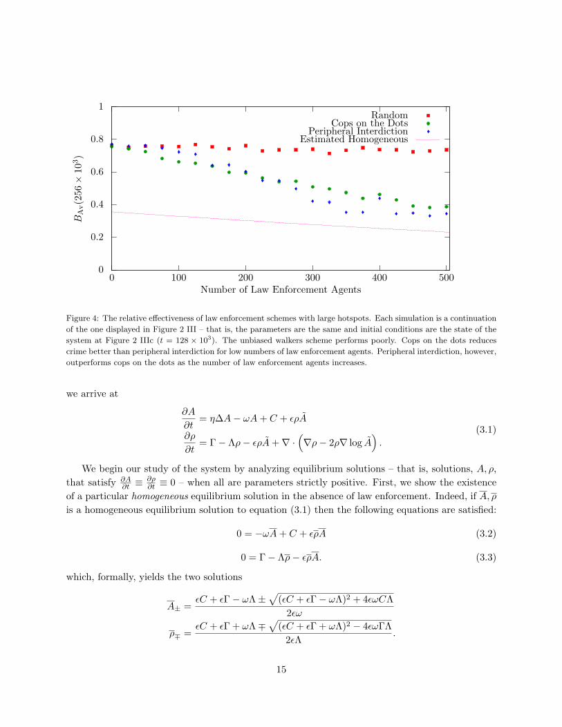
Figure 4: The relative effectiveness of law enforcement schemes with large hotspots. Each simulation is a continuation

of the one displayed in Figure 2 III – that is, the parameters are the same and initial conditions are the state of the

system at Figure 2 IIIc (t = 128 × 103). The unbiased walkers scheme performs poorly. Cops on the dots reduces

crime better than peripheral interdiction for low numbers of law enforcement agents. Peripheral interdiction, however,

outperforms cops on the dots as the number of law enforcement agents increases.

we arrive at

∂A

∂t= η∆A− ωA+ C + ερA

∂ρ

∂t= Γ− Λρ− ερA+∇ ·

(∇ρ− 2ρ∇ log A

).

(3.1)

We begin our study of the system by analyzing equilibrium solutions – that is, solutions, A, ρ,that satisfy ∂A

∂t ≡ ∂ρ∂t ≡ 0 – when all are parameters strictly positive. First, we show the existence

of a particular homogeneous equilibrium solution in the absence of law enforcement. Indeed, if A, ρis a homogeneous equilibrium solution to equation (3.1) then the following equations are satisfied:

0 = −ωA+ C + ερA (3.2)

0 = Γ− Λρ− ερA. (3.3)

which, formally, yields the two solutions

A± =εC + εΓ− ωΛ±√(εC + εΓ− ωΛ)2 + 4εωCΛ

2εω

ρ∓ =εC + εΓ + ωΛ∓√(εC + εΓ + ωΛ)2 − 4εωΓΛ

2εΛ.

15

(a) t = 1× 103

ACA = 1784

BAv = 0.734

(b) t = 8× 103

ACA = 1829

BAv = 0.733

(c) t = 64× 103

ACA = 1772

BAv = 0.721

(I) Unbiased Walkers. This method

is largely ineffective in criminal ac-

tivity. Crime hotspots persist de-

spite law enforcement intervention.

Only a small reduction in criminal

activity, BAv(64 × 103) = 0.721, is

observed from the initial attractive-

ness, BAv(0) = 0.751.

(a) t = 1× 103

ACA = 2247

BAv = 0.604

(b) t = 8× 103

ACA = 2481

BAv = 0.513

(c) t = 64× 103

ACA = 2397

BAv = 0.515

(II) Cops on the Dots. Criminal ac-

tivity is reduced. The intensity of

crime hotspots has been lowered.

There has been a fair reduction in

criminal activity, BAv(64 × 103) =

0.515 a decrease from the initial

value of BAv(0) = 0.751.

(a) t = 1× 103

ACA = 1997

BAv = 0.682

(b) t = 8× 103

ACA = 2394

BAv = 0.519

(c) t = 64× 103

ACA = 2500

BAv = 0.523

(III) Peripheral Interdiction. Crimi-

nal activity has been reduced. Some

crime hotspots have been eradicated

and the remaining ones have lower

intensity. Criminal Activity is re-

duced: BAv(64× 103) = 0.523 com-

pared with BAv(0) = 0.751.

Figure 5: Subfigures I, II, and III compare the relative effectiveness of different law enforcement strategies on a

system with pre-existing hotspots. In each case, 300 law enforcement agents are added. To make a law enforcement

agent 99% effective at preventing crime at its current site, χ = 4.605170. The simulations are continuations of the

simulation displayed in Figure 2 II – that is, the parameters are the same and initial conditions are the state of the

system at Figure 2 IIc (t = 128×103). The unbiased walker patrol method performs the worst. Cops on the dots and

peripheral interdiction are roughly comparable after some time, but latter method is less effective for short times.

Note that a peculiar side effect of our model is that a reduction in crime is associated with an increase in active

criminal agents. This is a result of the fact that fewer criminals committing burglaries implies fewer criminals are

being removed from the system.

16

(a) t = 8× 103

ACA = 1785

BAv = 0.733

(b) t = 32× 103

ACA = 1803

BAv = 0.738

(c) t = 128× 103

ACA = 1703

BAv = 0.754

(I) Unbiased Walkers. This method

is ineffective in reducing criminal ac-

tivity. Crime hotspots persist de-

spite law enforcement intervention.

There is a slight increase in the at-

tractiveness, BAv(64×103) = 0.754,

is observed from the initial value,

BAv(0) = 0.728.

(a) t = 8× 103

ACA = 2199

BAv = 0.647

(b) t = 32× 103

ACA = 2559

BAv = 0.515

(c) t = 128× 103

ACA = 2389

BAv = 0.524

(II) Cops on the Dots. Criminal ac-

tivity is reduced. The intensity of

crime hotspots has been lowered.

There has been a fair reduction in

the attractiveness, BAv(64× 103) =

0.524, a decrease from the initial

value of BAv(0) = 0.728.

(a) t = 8× 103

ACA = 2136

BAv = 0.675

(b) t = 32× 103

ACA = 2438

BAv = 0.523

(c) t = 128× 103

ACA = 2814

BAv = 0.410

(III) Peripheral Interdiction. Crimi-

nal activity has been reduced. The

crime hotspots have been eradi-

cated. The attractiveness has been

dramatically lowered: BAv(64 ×103) = 0.410 compared with

BAv(0) = 0.728.

Figure 6: Subfigures I, II, and III compare the relative effectiveness of different law enforcement strategies on a system

with pre-existing hotspots. In each case, we add 300 law enforcement agents. We set χ = 4.605170; this implies that

one law enforcement agent is 99% effective at preventing crime at its current site. The simulations are continuations

of the simulation displayed in Figure 2 III – that is, they share the same parameters and initial conditions as the

state of the system at Figure 2 IIIc (t = 128×103). Again, the unbiased walkers scheme is ineffective. Although cops

on the dots performs slightly better for short periods of time, peripheral interdiction is the best method in the long

run.

17

However sinceεC + εΓ− ωΛ <

√(εC + εΓ− ωΛ)2 + 4εωCΛ,

A− < 0 and hence “aphysical” (i.e., does not correspond to an actual situation). We may thereforeeliminate from consideration the pair (A−, ρ+) and have thus proved the following:

Proposition 3.1 If κ(x, t) ≡ 0, and Γ,Λ, C, ε, and ω are positive then there is a unique spatiallyhomogeneous solution of equation(3.1) given by

A =εC + εΓ− ωΛ +

√(εC + εΓ− ωΛ)2 + 4εωCΛ

2εω(3.4)

ρ =εC + εΓ + ωΛ−√(εC + εΓ + ωΛ)2 − 4εωΓΛ

2εΛ. (3.5)

We are now in a position to examine the effect of law enforcement agents on the equilibriumsolution. Suppose that the law enforcement agents are patrolling randomly, that is they are evolvingaccording to equation (2.6).

Eventually, the law enforcement agent density tends to a constant – that is, κ(x, t) = κ0 – andit is seen that in the system (3.1) we may remove all tildes at the expense of ε→ e−κ0χε. Therefore,with the random strategy, an increase in the number of law enforcement agents is equivalent toa decrease in ε. The purpose of adding law enforcement agents to the system was to reduce theamount of crime being committed. Thus, as far as the random strategy is concerned, this amountsto showing that a decrease in ε causes a reduction in crime. First, we must pause to determine howto define “reduction in crime”.

In equilibrium, the total attractiveness of the system ‖A‖L1 is a linearly related to the rate ofburglaries as can be seen directly from Eq.(3.2). Moreover, with periodic or Neumann boundaryconditions, this is true for long time averages – appropriate limits taken. Indeed, integrating andaveraging:

∂A

∂t= η∆A− ωA+ C + εAρ = 0,

〈‖A‖L1〉 =1ω

(C + 〈‖εAρ‖L1〉) .which is just the equilibrium result. Thus in what follows, we will consider a reduction in A to beequivalent to a reduction in criminal activity.

Since in this section we are concerned with the effect of law enforcement and we have shown therelationship between ε and the equilibrium number of cops, from this point forward we will treatε ∈ R+ as a parameter. And we will treat various variables as functions of ε when convenient.

The following lemma proves in part a weak version of the statement that an addition of lawenforcement officers causes a reduction in the amount of criminal activity.

Lemma 3.2 The equilibrium solution, A, is an increasing function of ε. Likewise, the equilibriumsolution, ρ, is a decreasing function of ε.

18

Proof. By differentiating equation (3.4) with respect to ε we see that

∂A

∂ε=

Λ

2ε2√(

C + Γ− ωΛε

)2 + 4ωΛε C

√(C + Γ− ωΛε

)2

+ 4ωΛεC − C + Γ− ωΛ

ε

>

Λ

2ε2√(

C + Γ− ωΛε

)2 + 4ωΛε C

[∣∣∣∣C − Γ +ωΛε

∣∣∣∣− ∣∣∣∣C − Γ +ωΛε

∣∣∣∣]≥ 0.

The first inequality follows from(C + Γ− ωΛ

ε

)2

+ 4ωΛεC >

(C + Γ− ωΛ

ε

)2

+ 4ωΛεC − 4CΓ

=(C − Γ +

ωΛε

)2

.

It is noted directly from the combination of Eqs.(3.2)–(3.3) that since ωA+ Λρ is constant thenif one increases the other decreases. Nevertheless, we attack ρ directly:

∂ρ

∂ε= − ω

2ε2√(

C + Γ + ωΛε

)2 − 4ωΛε

√(C + Γ +ωΛε

)2

− 4ωΛε− C + Γ− ωΛ

ε

.< − ω

2ε2√(

C + Γ + ωΛε

)2 − 4ωΛε

[∣∣∣∣C − Γ +ωΛε

∣∣∣∣− ∣∣∣∣C − Γ +ωΛε

∣∣∣∣]≤ 0.

Where the first equality follows from(C + Γ +

ωΛε

)2

− 4ωΛε>

(C + Γ +

ωΛε

)2

− 4ωΛε− 4ΓC =

(C − Γ +

ωΛε

)2

.

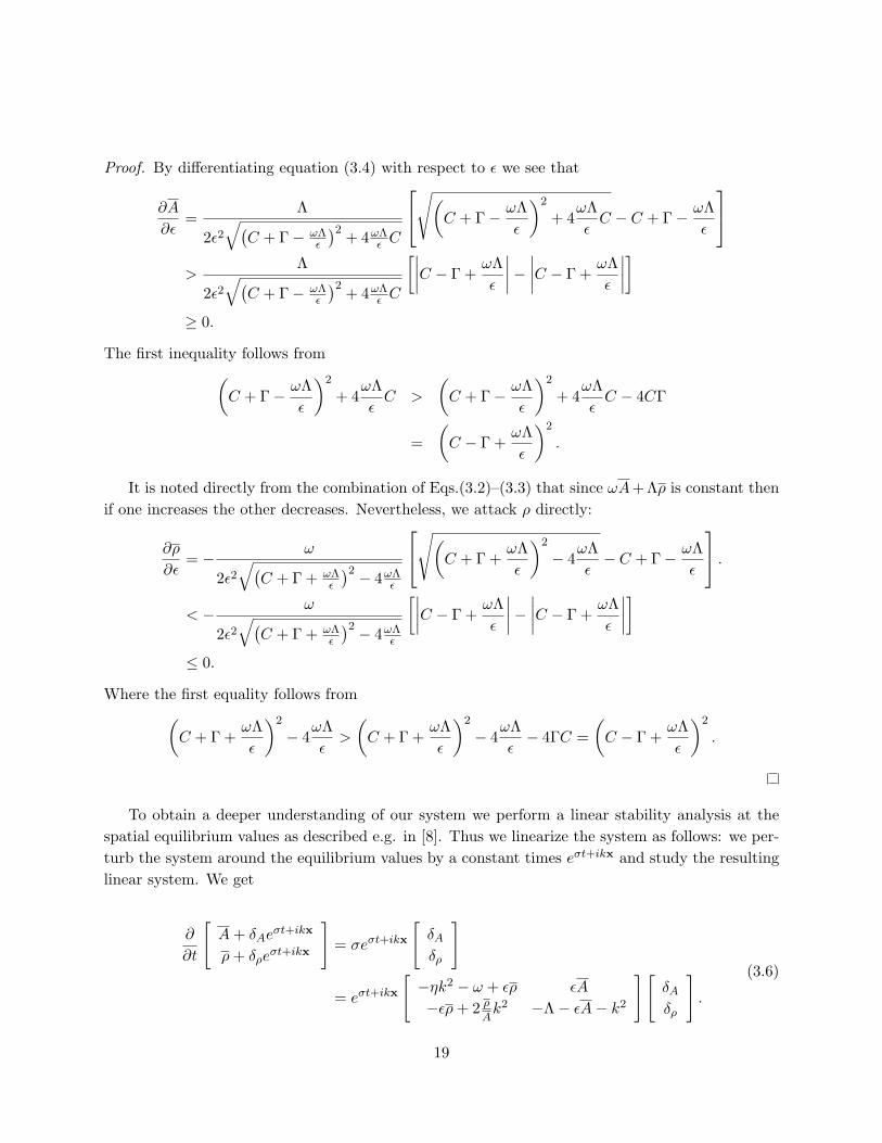
To obtain a deeper understanding of our system we perform a linear stability analysis at thespatial equilibrium values as described e.g. in [8]. Thus we linearize the system as follows: we per-turb the system around the equilibrium values by a constant times eσt+ikx and study the resultinglinear system. We get

∂

∂t

[A+ δAe

σt+ikx

ρ+ δρeσt+ikx

]= σeσt+ikx

[δAδρ

]

= eσt+ikx

[−ηk2 − ω + ερ εA

−ερ+ 2 ρAk2 −Λ− εA− k2

][δAδρ

].

(3.6)

19

By studying the eigenvalues of the above matrix we can determine when the system is linearlyunstable. The two eigenvalues of the system are

λ± = TrM

2±√(

TrM

2

)2

− detM,

where M is the 2× 2 matrix featured in equation (3.6).Tr M < 0 as −Λ− εA− k2 < 0 and

−ηk2 − ω + ερ = −ηk2 − C

A< 0

where the equality in the above display follows from equation (3.2). Since λ− < 0 the spatialequilibrium is stable – that is λ+ > 0 if and only if detM < 0. A simple calculation shows that

detM = ηk4 +(C

A+ ηΛ + ηεA− 2ερ

)k2 + Λ

C

A+ εC + ε2ρA. (3.7)

For the time being we will ignore the question of when the spatially homogeneous equilibrium isunstable and only assert that unstable regions exist. Instead we will consider how an unstablesystem behaves as ε is changed.

Theorem 3.3 Consider fixed constants η, ω, C,Γ,Λ > 0. Then there exists constants ε1, ε2 so thatif ε < ε1 or ε > ε2 then the solution A(ε), ρ(ε) is linearly stable.

Proof. To show that a spatially homogeneous solution, A(ε), ρ(ε), is stable we must prove thatdetM(ε) > 0 for all k. Note that the terms which are quartic and constant in k are manifestlypositive. Thus it is enough to show that for ε sufficiently small/large the coefficient of k2 is alsopositive. We use the facts:

limε→0

A(ε) =C

ωand lim

ε→0ρ(ε) =

ΓΛ, (3.8)

we can see that

limε→0

(C

A+ ηΛ + ηεA− 2ερ

)= (ηΛ + ω)

Thus by the continuity there exists ε1 > 0, such that the object under the limit is positive for0 < ε < ε1 which implies that for all k, detM(ε) > 0. This completes one half of the proof.

Since

limε→∞

ερ(ε) =2ωΓΛC + Γ

and

limε→∞

A(ε) =C + Γω

,

it is clear thatlimε→∞

C

A(ε)+ ηΛ + ηεA(ε)− 2ερ(ε) =∞.

20

Thus there exists ε2 > 0 so that for ε > ε2 we have

C

A(ε)+ ηΛ + ηεA(ε)− 2ερ(ε) > 0

and thus, for all k, detM(ε) > 0 for ε > ε2.

Under most conditions, and by most criteria, the presence of law enforcement agents has thedesired effect of reducing criminal activity. However with special regards to the ε > ε2 portionof the preceding, the preliminary implication is that the addition of law enforcement agents candestabilize a quiescent environment. The statement must be quantified:

1. Although in this regime crime hotspots do emerge with the injection of law enforcementagents – thereby exhibiting increased criminal activity in certain locales – it appears that theoverall level of criminal activity actually decreases. Indeed, numerical simulations suggestmonotonicity of the total amount of crime with respect to ε. Figure 7 clearly shows that‖A(·, ε)‖L1 is increasing in ε.

2. While no attempt has been in this work to calibrate the simulation dynamics with actualcrime statistics, in the authors’ opinion the worst (domestic) scenarios roughly correspond tothe vicinity of ε = ε1. The activity level for ε ≥ ε2 may correspond to circumstances wheredrastic alternative modes of response must be considered.

We have seen that, under the full dynamics, cops on the dots tends to outperform the randomstrategy. By and large, this trend persists with regards to the stability analysis; especially undercircumstances of “limited resources”.

Theorem 3.4 Let A, ρ, κ be a spatially homogeneous equilibrium solution of equations (3.1) and(2.6). If the solution is stable and χκ < ΛC

4Γω then A, ρ, κ is a a stable solution of equations (3.1)and (2.7).

We start with a preliminary result:

Lemma 3.5 Suppose f(x) is a monic cubic polynomial satisfying

f(x) = (x+A)(x2 +Bx+ C

)A,B,C > 0. (3.9)

If h(x) ≡ f(x) +DAx+αDA2 where α > 1, D > 0, and (α− 1)D < B then h(x) can be written inthe form

h(x) = (x+ E)(x2 + Fx+G

)E,F,G > 0. (3.10)

Proof. Let g(x) ≡ DAx + αDA2. First we note that limx→−∞ h(x) = −∞. As h(−A) = (α −1)DA2 > 0 we see that h(x) has a root, x0, in [−∞,−A). Let E = −x0 > A > 0. Since h(0) =EG = AC + αDA2, we have

G =h(0)E

<AC + αDA2

A= C + αDA < DA+AB + C = h′(0) = EF +G.

21

0

10000

20000

30000

40000

50000

60000

0.0001 0.001 0.01 0.1 1

‖A‖ L

1

ε

Stable Region Unstable Region Stable Region

Numerical SolutionSpatially Homogeneous Solution

Figure 7: Shows the relationship between the actual and predicted levels of attractiveness. Each numerical simulation

was run with parameters η = 0.0125, θ = 1.0, ω = 3×10−3, Γ = 4×10−3, and Λ = 4×10−3 on Ω = [0, 200]×[0, 200] ⊂R2 with Neumann boundary conditions. The system was run to equilibrium. The formation of crime hotspots causes

total level of crime to be much larger than the spatially homogeneous level for some values of ε.

where the last inequality follows from (α − 1)D < B. Thus we see that F > 0. Finally, we notethat

G =h(0)E

> 0.

to complete the proof.

Proof of Theorem 3.4. We begin by perturbing the system around its equilibrium values. We have

∂

∂t

A+ δAeσt+ikx

ρ+ δρeσt+ikx

κ+ δκeσt+ikx

= σeσt+ikx

δAδρδκ

= eσt+ikx

−ηk2 − ω + εe−χκρ εe−χκA −χεAe−χκρ−εe−χκρ+ 2 ρ

Ak2 −Λ− εe−χκA− k2 χεAe−χκρ− 2χρk2

2 κAk2 0 −k2

δAδρδκ

.(3.11)

We denote the matrix in (3.11) N and the 2×2 upper-left sub-matrix of N as M . Thus characteristicpolynomial of N , pN (λ), is

pN (λ) = −(λ+ k2)pM (λ)− 2χκεe−χκρk2(3k2 + λ

). (3.12)

22

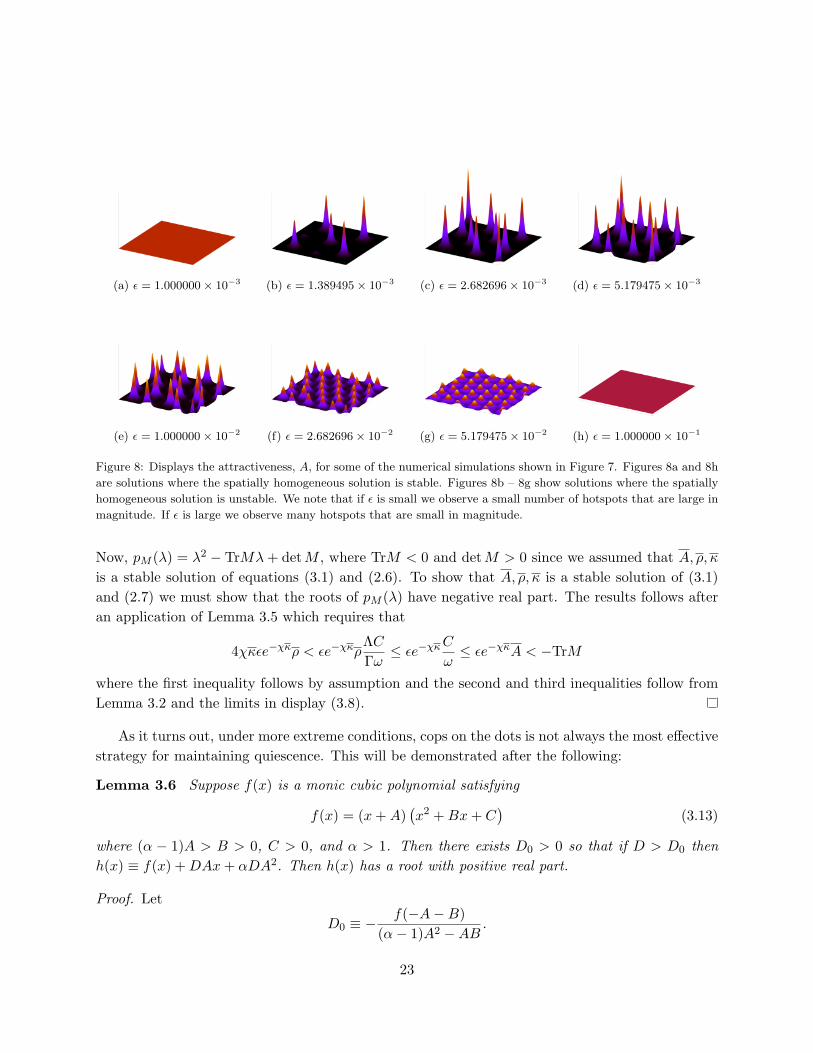
(a) ε = 1.000000× 10−3 (b) ε = 1.389495× 10−3 (c) ε = 2.682696× 10−3 (d) ε = 5.179475× 10−3

(e) ε = 1.000000× 10−2 (f) ε = 2.682696× 10−2 (g) ε = 5.179475× 10−2 (h) ε = 1.000000× 10−1

Figure 8: Displays the attractiveness, A, for some of the numerical simulations shown in Figure 7. Figures 8a and 8h

are solutions where the spatially homogeneous solution is stable. Figures 8b – 8g show solutions where the spatially

homogeneous solution is unstable. We note that if ε is small we observe a small number of hotspots that are large in

magnitude. If ε is large we observe many hotspots that are small in magnitude.

Now, pM (λ) = λ2 − TrMλ+ detM , where TrM < 0 and detM > 0 since we assumed that A, ρ, κis a stable solution of equations (3.1) and (2.6). To show that A, ρ, κ is a stable solution of (3.1)and (2.7) we must show that the roots of pM (λ) have negative real part. The results follows afteran application of Lemma 3.5 which requires that

4χκεe−χκρ < εe−χκρΛCΓω≤ εe−χκC

ω≤ εe−χκA < −TrM

where the first inequality follows by assumption and the second and third inequalities follow fromLemma 3.2 and the limits in display (3.8).

As it turns out, under more extreme conditions, cops on the dots is not always the most effectivestrategy for maintaining quiescence. This will be demonstrated after the following:

Lemma 3.6 Suppose f(x) is a monic cubic polynomial satisfying

f(x) = (x+A)(x2 +Bx+ C

)(3.13)

where (α − 1)A > B > 0, C > 0, and α > 1. Then there exists D0 > 0 so that if D > D0 thenh(x) ≡ f(x) +DAx+ αDA2. Then h(x) has a root with positive real part.

Proof. Let

D0 ≡ − f(−A−B)(α− 1)A2 −AB .

23

Then for D > D0 we have

h(−A−B)) = f((−A−B) +DA2 −DA(A+B) > 0.

We also note thath(−αA) = f(−αA) < 0

since the assumption B < (α − 1)A implies that any real root of f(x) is greater than (1− α)A asthe smallest real root of x2 +Bx+C is bounded below by −B. Thus h(x) has a root, x0, satisfyingx0 ∈ (−αA,−A−B). Now indeed we can write h(x) in the form

h(x) = (x− x0)(x2 + Fx+G)

for some constants F,G. But since

−x0 + F = h′′(0) = f ′′(0) = A+B,

we must haveF = x0 +A+B < (−A−B) +A+B < 0.

Thus h(x) has a root with positive real part.

With Lemma 3.6 we can show that cops on the dots is not always linearly stable when therandom patrol method is linearly stable. If η < 1 we can choose k2 such that −TrM < 2k2. Bychanging κ, χ and ε we can make the factor in equation 3.12

2χκεe−χκρ

arbitrarily large while keeping εe−χκ, and thus every other term, constant. Thus we can applyLemma 3.6 with D = 2χκεe−χκρ to get the result. However, we reemphasize that the circumstancesof this “exchanged stability” are not likely to correspond to realistic urban scenarios.

4 Summary

In this paper, we have examined the impact of introducing police into models involving mobilecriminal offenders and stationary targets, which are known to generate crime hotspot patterns. Westudied both discrete agent-based models and related continuum models and find that the intro-duction of structured policing strategies can eradicate crime hotspots. Specifically, so-called “copson the dots” is an effective strategy for eliminating smaller hotspots, while so-called “peripheralinterdiction” is more effective with larger hotspots. A baseline comparison shows that randompatrol does not lead to effective hotspot dissipation. Combined, our results suggest that it may bepossible to design spatial policing strategies from first principles.

24

Acknowledgments

This work benefitted immensely from the constructive criticism of Professor Andrea Bertozzi andthe advice of Professor Chris Anderson. This research was supported by the NSF under the grantDMS–03–06167 and, for L.C., DMS–08–054856.

References

[1] L. Anselin, J. Cohen, D. Cook, W. Gorr and G. Tita, Criminal Justice 2000, Vol. 4 (NationalInstitute of Justice, 2000), pp. 213-262.

[2] D. Beavon, P. L. Brantingham and P. J. Brantingham, Crime Prevention Studies, Vol. 2 (WillowTree Press, 1994), pp. 115-148.

[3] N. Bellomo, A. Bellouquid, J. Nieto and J. J. Soler, Multicellular growing systems: Hyperboliclimits towards macroscopic description, Math. Mod. Meth. Appl. Sci. 17 (2007) 1675-1693.

[4] M. Bendahmame, K. H. Karlsen and J. M. Urbano, On a two-sidely dengenerate chemotaxismodel with volume-filling effects, Math. Mod. Meth. Appl. Sci. 17 (2007) 783-804.

[5] W. Bernasco and F. Luykx, Effects of attractiveness, opportunity and accessibility to burglarson residential burglary rates of urban neighborhoods, Brit. J. Criminology 45 (2005) 296-315.

[6] W. Bernasco and P. Nieuwbeerta, How Do Residential Burglars Select Target Areas? TheBritish Journal of Criminology, 45, (2005) 297-315.

[7] A. E. Bottoms and P. Wiles, Crime, Policing and Place: Essays in Environmental Criminology(Routledge, 1992), pp. 11-35.

[8] J. P. Boyd, Chebyshev and Fourier Spectral Methods, 2nd edn. (Dover, 2001).

[9] A. Braga, The Effects of Hot Spots Policing on Crime Annals of the American Academy ofPolitical and Social Science, Vol. 578, What Works in Preventing Crime? Systematic Reviewsof Experimental and Quasi-Experimental Research, (2001) 104-125.

[10] P. J. Brantingham and P. L. Brantingham, Patterns in Crime (Macmillan, 1984).

[11] P. J. Brantingham and P. L. Brantingham, Environmental Criminology, 2nd edn. (WavelandPress, 1991), pp. 27-54.

[12] P. J. Brantingham and P. L. Brantingham, Criminality of place: Crime generators and crimeattractors, Euro. J. Criminal Policy Res. 3 (1995) 4-26.

25

[13] M. Burger, M. Di Francesco and Y. Dolak-Struss, The Keller-Segel model for chemotaxis withprevention of overcrowding: Linear vs. nonlinear diffusion, SIAM J. Math. Anal. 38 (2006)1288-1315.

[14] H. M. Byrne and M. R. Owen, A new interpretation of the Keller-Segel model based on multi-phase modelling, J. Math. Biol. 49 (2004) 604-626.

[15] F. A. Chalub, IY. Dolak-Struss, P. Markowich, D. Oeltz, C. Schmeiser and A. Soref, Modelhierarchies for cell aggregation by chemotaxis, Math Mod Meth. Appl. Sci. 16 (2006) 1173.

[16] F. A. Chalub, P. A. Markovich, B. Perthame and C. Scheiser, Kinetic models for chemotaxisand their drift-diffusion limits, Mon. Math. 142 (2004) 123.

[17] L. Cohen and M. Felson, Social-Change And Crime Rate Trends - Routine Activity ApproachAmerican Sociological Review 44, (1979) 588-608.

[18] M. C. Cross and P. C. Hohenberg, Pattern formation outside of equilibrium, Rev. Mod. Phys.65 (1993) 851-1112.

[19] M. del Pino and J. Wei, Collapsing steady states of the Keller-Segel system, Nonlinearity 19(2006) 661-684.

[20] Y. Dolak and C. Schmeiser, Kinetic models for chemotaxis: Hydrodynamics limits and spatiotemporal mechanisms J. Math. Biol. 51 (2005) 595-615.

[21] R. Erban and H. G. Othmer, From individual to collective behavioiur in chemotaxis, SIAM J.Appl. Math 65 (2004) 361-391.

[22] C. Escudero, The fractional Keller-Segel model, Nonlinearity 19 (2006) 2909-2918.

[23] M. K. Felson, Crime and Nature Sage Publications, 2006).

[24] F. Filbet, P. Laurencot and B. Perthame, Derivation of hyperbolic models for chemosensitivemovement, J. Math. Biol. 50 (2005) 189-207.

[25] Gottfredson, Michael R., and Travis Hirschi, A General Theory of Crime. Stanford UniversityPress, Stanford, California (1990).

[26] M. A. Herrero and J. J. L. Velazquez, Chemotactic collaspse for the Keller-Segel model, J.Math. Biol. 35 (1996) 177-194.

[27] S. D. Johnson, W. Bernasco, K. J. Bowers, H. Elffers, J. Ratcliffe, G. Rengert and M. Townsley,Space-time patterns of risk: A cross national assessment of residential burglary victimization,J. Quantitative Criminology 23 (2007) 201-219.

[28] S. Johnson, K. Bowers, and A. Hirschfield, New insights into the spatial and temporal distri-bution of repeat victimisation, The British Journal of Criminology 37, (1997) 224.

26

[29] K. Keizer, S. Lindenberg and L. Steg, The Spreading of Disorder Science:1161405, (2008).

[30] E. F. Keller and L. A. Segel, Initiation of slime mold aggregation viewed as an instability, J.Theor. Biol. 26 (1970) 399-415.

[31] G. Kelling, T. Pate, D. Dieckman, and C.E. Brown The Kansas City Preventive Patrol Exper-iment: A Summary Report Washington, D.C.: Police Foundation, (1974).

[32] M. Lewis, K. White and J. Murray, Analysis of a model for wolf territories, J. Math. Biol. 35(1997) 749-774.

[33] S. Luckhaus and Y. Sugiyama, Large time behavior of solutions in super-critical cases to de-generate Keller–Segel systems, Math. Model. Numer. Anal. 40 (2006) 597-621.

[34] L. McLaughlin, S. D. Johnson, D. Birks, K. J. Bowers, and K. Pease, Police perceptions of thelong and short term spatial distributions of residential burglary, Int. J. Police Sci. Management9 (2007) 99-111.

[35] P.R. Moorcroft, M.A. Lewis and R. Crabtree, Mechanistic home range models predict patternsof coyote territories in yellowstone, Proc. Roy. Soc. London B 273 (2006) 1651-1659.

[36] H.G. Othmer and T. Hillen, The diffusion limit of transport equations II: Chemotaxis equations,SIAM J. Appl. Math. 62 (2002) 1222-1250.

[37] J. H. Ratcliffe, Crime mapping and the training needs of law enforcement, Eur. J. CriminalPolicy Res. 10 (2004) 65-83.

[38] G. F. Rengert, Crime, Policing and Place: Essays in Environmental Criminology, (Routledge,1992), pp. 109-117.

[39] G. Rengert, Alex Piquero and P. Jones, Distance Decay Reexamined Criminology, 37, (1999)427-446.

[40] D. Roncek, and R. Bell, Bars, blocks and crime, J. Environ. Sys. 11 (1981) 35-47.

[41] T. Senba, Type II blowup of solutions to a simplified Keller–Segel system in two–dimensionaldomains, Nonlinear Anal. Th. Meth. Appl. Int. Multidisciplinary J. Ser. A: Th. Meth 66 (2007)1817-1839.

[42] M. B. Short, M. R. D’Orsogna, V. B. Pasour, G. E. Tita, P. J. Brantingham, A. L. Bertozzi,and L. B. Chayes, A Statistical Model of Criminal Behavior Mathematical Models and Methodsin Applied Sciences, 18, Suppl. (2008).

[43] B. Snook, Individual Differences in Distance Travelled by Serial Burglars Journal of Investiga-tive Psychology and Offender Profiling, 1 (2004) 53-66.

27

[44] H. Spohn, Large Scale Dynamics of Interacting Particles, Texts and Monographs in Physics,Springer–Verlag, Heidelberg, New York (1991).

[45] A. Stevens, The derivation of chemotaxis equations as limit dynamics of moderately interactingstochastic many–particle systems, SIAM J. Appl. Math. 61 (2002) 183-212.

[46] Y. Sugiyama, Global existence in sub–critical cases and finite blow–up in super–critical casesto degenerate Keller–Segel systems, Differential and Integral Equations Int. J. Th. Appl. 19(2006) 841-876.

[47] J. J. L. Velazquez, Well–posedness of a model of point dynamics for a limit of the Keller-Segelsystem, J. Diff. Eqs. 206 (2004) 315-352.

[48] W. F. Walsh, Compstat: An analysis of an emerging police and neighborhood safety, AtlanticMon. 249 (19822002) 29-38.

[49] D. Weisburd and J. E. Eck, What Can Police Do to Reduce Crime, Disorder, and Fear? TheANNALS of the American Academy of Political and Social Science, 593, (2004) 42-65.

[50] J. Wilson and G. Kelling, Broken windows and police and neighborhood safety, Atlantic Mon.249, (1982) 29.

[51] R. Wright and S. Decker, Burglars on the Jobs (Northeastern University Press, Boston, 1994).

[52] Federal Bureau of Investigation - Uniform Crime Reports, http://www.fbi.gov/ucr/ucr.htm(Dec 10, 2008).

28