Embed Size (px)
Citation preview
Statistical Modelling of EqualRisk Portfolio Optimization withEmphasis on Projection Methods
Master ThesisJune 2015
Sabrina Neumann
Aalborg UniversityDepartment of Mathematical SciencesIn collaboration with Department of Business & Management
Autumn 2014/Spring 2015

Department of Mathematical SciencesFredrik Bajers Vej 7G
9220 Aalborg ØTelephone 99 40 99 40
Fax 9940 3548http://www.math.aau.dk/
Title:Statistical Modelling of EqualRisk Portfolio Optimization withEmphasis on Projection Methods
Project period:September 2, 2014 -June 10, 2015
Author:Sabrina Neumann
Supervisors:Torben TvedebrinkLasse Bork
Circulation:7
Number of pages:118
Completed:June 10, 2015
Synopsis:
The objective of this thesis is to in-vestigate the Equal Risk asset al-location strategy that makes useof latent risk factors in a portfo-lio. This strategy can be consid-ered from different points of view,but in general it aims to equal-ize the risk contributions of theassets in a portfolio. There isplaced much emphasis on projec-tion methods such as principal com-ponent analysis and its functionalvariant, functional principal compo-nent analysis, which are used to ex-tract the latent risk factors. For thepurpose of investigating the perfor-mance of the Equal Risk strategycompared to other allocation strate-gies, e.g. the Equally-Weighted orMinimum Variance strategy, there isconsidered a walk-forward backtestwith a rolling estimation window onhistorical data. Data is kindly pro-vided by Jyske Bank A/S and in-cludes different types of assets.
© Sabrina Neumann

Preface
This master thesis is written by Sabrina Neumann during the period from September2, 2014 to June 10, 2015. The thesis is composed at the Department of MathematicalSciences at Aalborg University in collaboration with the Department of Business andManagement at Aalborg University, and with Jyske Bank A/S in Silkeborg.
The thesis deals with investigating the Equal Risk allocation strategy that is basedon latent risk factors, where the emphasis is on projection methods. In order tobacktest the different allocation strategies, Jyske Bank A/S kindly provides datathat includes different types of assets and some R code, which are treated confiden-tially.
Bibliographical references in the thesis are done with [author,year], and these can befound in the bibliography at the end of the thesis before the appendix. Referencesto definitions, theorems, etc. which start with ’A’ refer to the appendix. All figuresand code are implemented with the software R.
It is expected that the reader has basic knowledge equivalent to a bachelor degree inMathematics and Statistics from Aalborg University. In addtion, basic knowledgewithin measure theory is an advantage.
I would like to thank my supervisors, Assistant Professor Torben Tvedebrink, De-partment of Mathematical Sciences at Aalborg Univeristy, and Assistant ProfessorLasse Bork, Department of Business and Management at Aalborg University, forfor their enthusiasm and great help during the thesis. I would also like to thankJyske Bank A/S for providing data, R code, and inside knowledge, and in particularAnders Hartelius Haaning for an introduction to the topic, and his great help andcommitment.
Sabrina NeumannAalborg, June 2015
v

Resumé
Formålet med denne specialeafhandling er at betragte aktivallokerings strategier,der er baseret på risikofaktorer i stedet for traditionelle strategier, der allokererved hjælp af aktivklasser. Motivationen for at betragte risiko-baserede strategierligger i problemstillingen at strategier der udelukkende er baseret på estimater afmiddelværdi og varians, som eksempelvis Markowitz mean-variance strategien, ikkekan fange den tunge venstre hale i afkastfordelingen i perioder af høj volatilitet,som for eksempel finanskrisen i 2008/2009. For at opnå en bedre forståelse af denøkonomiske tankegang bag risiko-baserede modeller, gives der en introduktion tilvigtige økonomiske faktor-baserede modeller, såsom Capital Asset Pricing Model,Arbitrage Pricing Theory og Fama og Frenchs tre faktor model.
For at kunne finde de underliggende risikofaktorer af en portefølje betragtes principalcomponent analysis, som er en statistisk metode til at transformere det oprindeligaktivrum i et lavere dimensionalt rum, der netop udgør risikofaktorerne. Dennemetode betragtes også fra en funktionel tilgang: functional principal componentanalysis. Her arbejdes med de samme principper som i principal component analysis,men det antages, at data har en underliggende funktionel from. Dermed arbejdesder med egenfunktioner, som observeres over tid i stedet for egenvektorer, der baregiver statiske og ikke-temporære estimater. For at kunne arbejde med functionalprincipal component analysis skal data transformeres til funktioner, hvilket gøresved hjælp af B-splines. Samtidig udglattes data ved at bruge en penalized weightedleast squares metode, hvilket øger signal-to-noise ratioen af data. Motivationenfor at betragte den funktionelle tilgang ligger i antagelsen om, at nøjagtigheden afallokerings strategierne kan øges. Derudover er det teoretisk set muligt at indkludereaktiver med forskellige samplingfrekvens i en portefølje, hvilket ikke er muligt i enmultivariat tilgang, hvor data betragtes som enkelte observationer.
Der fokuseres specielt på Equal Risk strategien, der kan betragtes med forskelligetilgange. Enten kan den betragtes som en optimering der har til formål at vælgeporteføljevægtene sådan, at risiko bidragene fra hvert enkelt aktiv er lige store.Eller den kan betragtes som en optimering, hvor vægtene af de enkelte aktiver i enportefølje vælges sådan, at en principal component analysis på de historiske afkast-serier giver så ens som mulig standardafvigelse i principal komponentretningerne.Equal Risk strategien sammenlignes med fast allokering, Equally-Weighted, og dentraditionelle Minimum Variance strategi.
vii
For at kunne sammenligne præstationen af de forskellige strategier betragtes enbacktest med rullende estimationsvindue på historiske afkastserier. Der undersøgesforskellige estimationsvinduer, og det antages, at short-selling ikke er tilladt. Back-testen baseres på tre forskellige portføljer, der indeholder flere aktivklasser samt etforskelligt antal af aktiver. Det observeres, at både længden af estimationsvinduetog sammensætningen af porteføljen har en indflydelse på den profit, der kan opnåsved de forskellige allokerings strategier. Der er lagt meget vægt på at undersøgeeffekten af at udelade nogle principal komponenter, det vil sige at betragte et min-dre antal underliggende risikofaktorer. Der findes ikke et entydig resultat for omdenne effekt har en positiv eller negativ indflydelse på allokerings strategierne, mendet har været muligt at øge profitten i en af porteføljerne ved at betragte et mindreantal principal komponenter. Desuden kan det konkluderes udfra backtesten, atEqually-Weighted strategien det meste af tiden har en højere profit end de andretestede strategier, men at den ikke performer godt igennem finanskrisen. Der er detnetop nogle af de betragtede risiko-baserede strategier, der performer stabilt, hvilketmotiverer brugen af disse strategier. Den funktionelle tilgang kan ikke outperformede andre risiko-baserede strategier igennem finanskrisen, men har i nogle porteføljesammensætninger en meget aktraktiv afkast i normale tider. Desuden har de risiko-baserede strategier en mindre volatil profit end Equally-Weighted strategien, hvilketer en vigtig egenskab for de fleste investorer.
viii
Contents
1 Introduction 11.1 Portfolio Theory . . . . . . . . . . . . . . . . . . . . . . . . . . . . . 2
1.1.1 Portfolio Mean and Variance, and other Measures of Risk . . . 41.2 Factor Models and Risk Factors . . . . . . . . . . . . . . . . . . . . . 7
1.2.1 The Capital Asset Pricing Model . . . . . . . . . . . . . . . . 71.2.2 Multifactor Models and the Arbitrage Pricing Theory . . . . . 13
2 Functional Data Analysis 192.1 Functional Data . . . . . . . . . . . . . . . . . . . . . . . . . . . . . . 20
2.1.1 Basis Functions . . . . . . . . . . . . . . . . . . . . . . . . . . 222.1.2 Smoothing Functional Data . . . . . . . . . . . . . . . . . . . 24
2.2 Principal Component Analysis . . . . . . . . . . . . . . . . . . . . . . 262.2.1 Singular Value Decomposition and the Smoothing of Data . . 28
2.3 Functional Principal Component Analysis . . . . . . . . . . . . . . . 292.3.1 Approximate Solution to Eigendecompostion . . . . . . . . . . 342.3.2 The Choice of the Number of Principal Components . . . . . . 36
3 Risk-based Allocation Strategies 393.1 Equal Risk Portfolio Optimization . . . . . . . . . . . . . . . . . . . . 39
3.1.1 Risk Contribution Approach . . . . . . . . . . . . . . . . . . . 403.1.2 Properties of the Equal Risk Strategy . . . . . . . . . . . . . . 433.1.3 Principal Component Analysis Approach . . . . . . . . . . . . 47
3.2 Diversified Risk Parity . . . . . . . . . . . . . . . . . . . . . . . . . . 523.3 The Equally-Weighted and Minimum Variance Strategies using Prin-
cipal Portfolios . . . . . . . . . . . . . . . . . . . . . . . . . . . . . . 543.4 Example . . . . . . . . . . . . . . . . . . . . . . . . . . . . . . . . . . 55
3.4.1 Principal Component Analysis . . . . . . . . . . . . . . . . . . 563.4.2 Functional Principal Component Analysis . . . . . . . . . . . 58
4 Backtest of Allocation Strategies 654.1 Portfolios . . . . . . . . . . . . . . . . . . . . . . . . . . . . . . . . . 66
4.1.1 Asset Classes . . . . . . . . . . . . . . . . . . . . . . . . . . . 664.1.2 Asset Classes and Style Factors . . . . . . . . . . . . . . . . . 684.1.3 Large Portfolio - 21 Assets . . . . . . . . . . . . . . . . . . . . 71
4.2 Backtest . . . . . . . . . . . . . . . . . . . . . . . . . . . . . . . . . . 75
ix

CONTENTS
4.2.1 Asset Classes . . . . . . . . . . . . . . . . . . . . . . . . . . . 774.2.2 Asset Classes and Style Factors . . . . . . . . . . . . . . . . . 894.2.3 Large Portfolio - 21 Assets . . . . . . . . . . . . . . . . . . . . 96
4.3 Review of the Backtest . . . . . . . . . . . . . . . . . . . . . . . . . . 100
5 Recapitulation 107
Bibliography 111
A Appendix 115A.1 Hilbert Spaces . . . . . . . . . . . . . . . . . . . . . . . . . . . . . . . 115A.2 Flow Chart: R Code . . . . . . . . . . . . . . . . . . . . . . . . . . . 118
x
Introduction 1This thesis deals with studying asset allocation strategies that are based on riskfactors instead of traditional strategies, that allocate by asset classes. This is mo-tivated by the fact that strategies which are entirely based on the estimates of themean and variance of assets, e.g. the Markowitz mean-variance strategy, cannotcapture the heavy left tail in the distribution of a return that occurs in times ofhigh volatility, e.g. during the recent financial crisis in 2008/2009.
The aim is to establish asset allocation strategies that are based on independent,underlying drivers of assets. These drivers are also called risk factors, which canbe classified into observable factors, e.g. growth or inflation, and latent factors thatare not observable. The focus in this thesis is on strategies that are based onlatent factors such that the risk of a portfolio is spread out to assets that do notall behave similar, especially during financial crises where many assets are likely tocrash. The emphasis is on the Equal Risk portfolio optimization strategy that canbe considered from different points of view, which will be investigated in this thesis.For the purpose of comparing the performance of the risk-based strategies thatwill be introduced, these strategies will be compared to the traditional MinimumVariance strategy and the simple Equally-Weighted strategy.
The mathematical tool used to extract the underlying, lower dimensional risk factorsis principal component analysis, which is a well-known tool in the field of statisticsto find linearly uncorrelated, i.e. independent, variables in data. In addition, thefunctional variant, functional principal component analysis, is considered in orderto explore possible improvements in the allocation strategies. Note that principalcomponent analysis should not be confused with factor analysis, which assumesthat there is an underlying model, since principal component analysis just is adimensionality reduction method.
In the recent years there is conducted some research of risk-based allocation strate-gies. [S. Maillard, T. Roncalli, J. Teiletche, 2009] introduces the general idea of theEqual Risk strategy and shows relations between the Equal Risk strategy to thetraditional Minimum Variance strategy and the simple Equally-Weighted strategy.[Kind, 2013] focuses on the risk-based strategies using principal component analysis,
1
CHAPTER 1. INTRODUCTION
and [Meucci, 2010] introduces a related strategy: Diversified Risk Parity, and ex-tensions are presented in [A. Meucci, A. Santangelo, R. Deguest, 2014]. This thesispresents among others some of the most important results of these articles.
But first in order to achieve a better understanding of the economical terminology,concepts, and models the following sections introduce the basic economical theoryfor factor models, their motivations and critics, the concept of diversification, andrisk premia.
1.1 Portfolio TheoryThis section introduces general concepts within portfolio theory and is inspired by[Luenberger, 2009]. The rate of return, r, of an asset over a single period is definedas:
r = X(1)−X(0)X(0) ,
where X(1) is the amount received and X(0) the amount invested. It is oftenassumed that prices are log-normally distributed, which implies that log returns,log(R), are given by:
log(R) = log(1 + r) = log(X(1)X(0)
)= log(X(1))− log(X(0)).
In order to form a portfolio, suppose that there are N different assets available inthe market. Let Xi(t) denote the price of asset i at time t, then the log returns,log(Ri(t)), are computed as follows:
log(Ri(t)) = log(Xi(t))− log(Xi(t−1)), for i = 1, . . . , N and t = 2, . . . , T, (1.1)
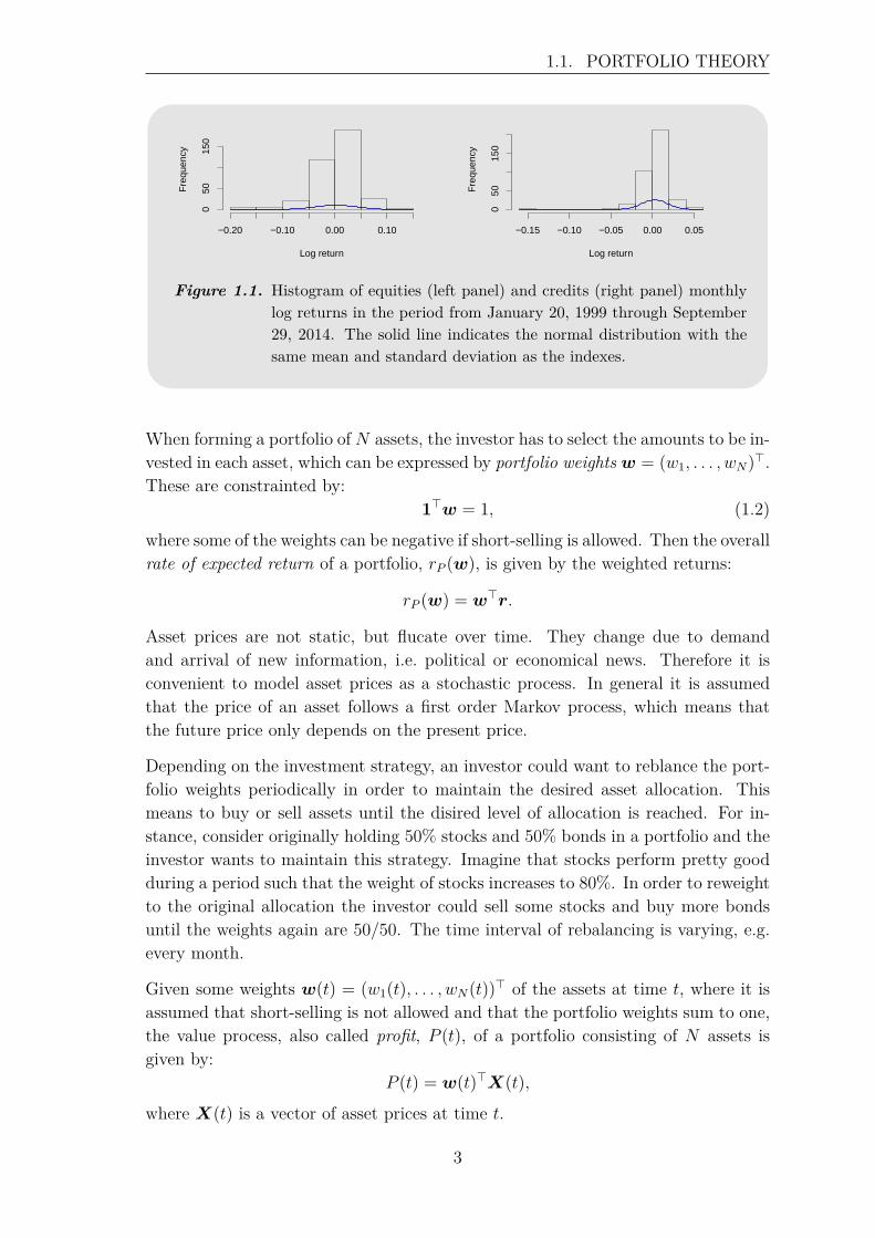
where log(Ri(1)) = 0 and T is the number of observations in the sampling periode.Both academics and practitioners often assume that asset log returns follow a normaldistribution, which is basis for many fields in finance. However, it can be observedthat real financial data often is more heavy tailed than the normal distribution, e.g.under crashes return distributions have a heavy left tail. [Longin, 2005] This canalso be observed in Figure 1.1, which shows histograms for the monthly log returnsof two indexes describing equities and credits, respectively.
2
1.1. PORTFOLIO THEORY
Log return − Equities
Log return
Fre
quen
cy
−0.20 −0.10 0.00 0.10
050
150
Log return − Credit
Log return
Fre
quen
cy
−0.15 −0.10 −0.05 0.00 0.05
050
150
Figure 1.1. Histogram of equities (left panel) and credits (right panel) monthlylog returns in the period from January 20, 1999 through September29, 2014. The solid line indicates the normal distribution with thesame mean and standard deviation as the indexes.
When forming a portfolio of N assets, the investor has to select the amounts to be in-vested in each asset, which can be expressed by portfolio weights w = (w1, . . . , wN)>.These are constrainted by:
1>w = 1, (1.2)
where some of the weights can be negative if short-selling is allowed. Then the overallrate of expected return of a portfolio, rP (w), is given by the weighted returns:
rP (w) = w>r.
Asset prices are not static, but flucate over time. They change due to demandand arrival of new information, i.e. political or economical news. Therefore it isconvenient to model asset prices as a stochastic process. In general it is assumedthat the price of an asset follows a first order Markov process, which means thatthe future price only depends on the present price.
Depending on the investment strategy, an investor could want to reblance the port-folio weights periodically in order to maintain the desired asset allocation. Thismeans to buy or sell assets until the disired level of allocation is reached. For in-stance, consider originally holding 50% stocks and 50% bonds in a portfolio and theinvestor wants to maintain this strategy. Imagine that stocks perform pretty goodduring a period such that the weight of stocks increases to 80%. In order to reweightto the original allocation the investor could sell some stocks and buy more bondsuntil the weights again are 50/50. The time interval of rebalancing is varying, e.g.every month.
Given some weights w(t) = (w1(t), . . . , wN(t))> of the assets at time t, where it isassumed that short-selling is not allowed and that the portfolio weights sum to one,the value process, also called profit, P (t), of a portfolio consisting of N assets isgiven by:
P (t) = w(t)>X(t),
where X(t) is a vector of asset prices at time t.
3
CHAPTER 1. INTRODUCTION
The processes (w1(t))t≥0 . . . , (wN(t))t≥0 are adapted, i.e. the weights are chosen ac-cording to the information available at time t. The process (w1(t) . . . , wN(t))t≥0 iscalled the portfolio strategy. [Lesniewski, 2008] The continuously compounded returnprofit using log returns is then computed by:
P (t+ 1) = P (t) · exp(w(t)> log(R(t))
),
where log(R(t)) is a vector of log returns at time t as defined in equation (1.1).[Zivot, 2015] From this the annulized geometrical mean profit, MP, is given by:
MP =(P (T )P (1)
) pT
− 1, (1.3)
where p indicates the number of periods per year, e.g. when dealing with monthlyobserved data p = 12. And the annulized volatility, Vol, of the profit is given by:
Vol =
√√√√√ 1T
T∑t=1
(P (t)− 1
T
T∑i=1
P (t))2
· √p. (1.4)
The next section introduces the general definitions of portfolio mean and variance,some basic asset allocation strategies, and other measures of risk for a portfolio.
1.1.1 Portfolio Mean and Variance, and other Measures ofRisk
With the purpose of measuring the performance of an asset allocation strategy theportfolio mean and variance often are considered. Portfolio optimization often isbased on maximizing the expected rate of return of a portfolio, µP (w), which isgiven by:
µP (w) = w>µ,
where µ = (µ1, . . . , µN)> is a vector of expected values of the N assets of a portfolio.Correspondingly, the variance of the rate of return of a portfolio, σ2
P (w), can bedetermined by:
σ2P (w) = E
[(rP (w)− µP (w))2
]= E
[w>(r − µ)(r − µ)>w
]= w>Σw, (1.5)
where Σ is the covariance matrix. The standard deviation of a portfolio’s rate ofreturn, σP (w), is usually used as a basic measure of risk:
σP (w) =√w>Σw. (1.6)
A higher standard deviation is associated with higher risk and higher risk is requiredto get a higher expected return. Thereby each investor is faced by the tradeoff of
4
1.1. PORTFOLIO THEORY
expected return and risk. Note that in financial context the standard deviation isoften called volatility and the two terms will be used interchangeably in this thesis.
The traditional Markowitz Mean-Variance, MV, asset allocation strategy aims tofind a portfolio, where the expected rate of return of the portfolio is fixed at someabitrary expected value µ while minimizing the portfolio variance:
min w>Σwsubject to w>µ = µ and 1>w = 1. (1.7)
This strategy is based on the assumption that asset returns are normal distributed, astrong assumption that as mentioned above often is violated for real data. Moreover,this allocation strategy assumes stable correlations of assets over time, which againis not met by most assets. Although these assumptions are likely to be violated, theMV strategy is widely used by both academics and the financial industry becauseof the ease of computations.
However, instead of focusing on the expected rate of return of a portfolio, whichoften is hard to estimate, other portfolio optimization methods consider themarginalrisk contribution, ∂wi
σP (w), of the ith asset. It is defined by:
∂wiσP (w) = ∂σP (w)
∂wi= (Σw)i√
w>Σw
=wiσ
2i +∑
i 6=j wjσijσP (w) . (1.8)
The marginal risk contributions explain the change in the volatility of a portfoliodue to a small increase in the weight of one component. [S. Maillard, T. Roncalli,J. Teiletche, 2009]
One strategy that uses this concept is the Minimum Variance strategy, MVa, whichis based on the assumption that the marginal risk contributions should be identicalacross the assets of a portfolio. [Kind, 2013] The MVa weights can be found bysolving:
minw
w>Σw (1.9)
subject to 1>w = 1.
Hence the MVa strategy is a special case of the MV strategy, when the requirementof the expected return is omitted.
But there are also strategies that assume that the risk contributions are equal, whichwill be introduced in Chapter 3. The risk contribution of the ith asset, RCi(w), canbe expressed as:
RCi(w) = wi · ∂wiσP (w) = wi
(Σw)i√w>Σw
. (1.10)
In order to show further properties of the risk contributions RCi(w) the followingdefinition introduces the concept of a homogeneous function.
5
CHAPTER 1. INTRODUCTION
Definition 1.1 (Homogeneous Function)A function f : X ⊂ RN → R is called a homogeneous function of degree τ ifthere exists a λ > 0 and x ∈ X, where λx ∈ X such that the following holds:
f(λx) = λτf(x).
[Tasche, 2008]
Furthermore, Theorem 1.2 introduces the Euler decomposition, which can be usedto show the relationship between the portfolio volatility σP (w) and the risk contri-butions RCi(w).
Theorem 1.2 (Euler’s Theorem on Homogeneous Functions)Let X ⊂ RN be an open set and let f : X → R be a continuously differentiablefunction. Then f is a homogeneous function of degree τ if and only if it satisfiesthe following:
τf(x) =N∑i=1
xi∂f(x)∂xi
,
where x ∈ X. [Tasche, 2008]
Proof. Omitted.
It is known that the volatility σP (w) is a homogeneous function of degree one, i.e.τ = 1 in Definition 1.1. Thus it satisfies Euler’s decompostion as given in Theorem1.2:
N∑i=1
RCi(w) =N∑i=1
wi(Σw)i√w>Σw
= w>Σw√w>Σw
=√w>Σw = σP (w)
This shows that the volatility of a portfolio can be decomposed into risk contri-butions of the included assets. After having introduced these basic concepts ofportfolio theory, the next section presents different economical theory concerningfactor models.
6
1.2. FACTOR MODELS AND RISK FACTORS
1.2 Factor Models and Risk FactorsFirst, this section gives a short introduction to the Capital Asset Pricing Model,CAPM, which is a one factor model that quantifies the tradeoff between expectedreturn and risk within the mean-variance framework. It was introduced indepen-dently by Treynor (1961), Sharpe (1964), Litner (1965), and Mossin (1966). [Ang,2014] The model involves a linear relationship between the expected return of anasset with the covariance of its return and the return of the market portfolio. [J. Y.Campbell, A. W. Lo, A. C. MacKinlay, 1997]
Furthermore in Section 1.2.2, the one factor CAPM model is expanded to a multi-factor model, the Arbitrage Pricing Model, APT, developed by Ross (1976). [Ang,2014] In this setup it is assumed that any risky asset can be considered as a linearcombination of various risk factors that affect the asset return. [T. E. Copelandand J. F. Weston, 1988] There are different types of risk factors, like macro factors,style factors, and firm-specific factors, which will be introduced. Furthermore theFama-French three factor model is shortly presented.
1.2.1 The Capital Asset Pricing ModelThis section introduces the one factor model CAPM and is inspired by [Luenberger,2009] and [M. Grinblatt and S. Titman, 2002]. In order to understand the CAPM,first the concept of the market portfolio is explained. The market portfolio M is atheoretical summation of all available assets of the world financial market, whereeach asset is weighted by its proportion in the market, i.e. its market value. Let videnote the market value of asset i, then the market weights, wMi , can be expressedby:
wMi = vi∑Ni=1 vi
.
Thereby the expected return of the market portfolio reflects the expected return ofthe market as a whole and it is assumed that the portfolio has the lowest volatilityamong all portfolio that have the same expected return as the market. This isthe same as saying that the market has the highest Sharpe ratio, which will beintroduced later in this section.
Assuming that all investors use the Markowitz mean-variance framework to de-termine their portfolio weights, that everyone invests in all available assets in themarket, and that there are no transactions costs, then the market portfolio M issaid to be the efficient portfolio in the market. This means that investors will recal-culate their estimates of the portfolio weights until demand matches supply, whichdrives the market to efficiency. Additionally, the CAPM assumes the existence of arisk-free asset, which represents the possibility of an investor to borrow or lend cashat the risk-free rate. Let rf be the return of a risk-free asset, which means that thereturn is deterministic. When included in a portfolio, a positive weight correspondsto lending cash, whereas a negative weight means borrowing cash.
7
CHAPTER 1. INTRODUCTION
The following result states that risk-averse investors will invest in a portfolio con-sisting of a combination of two portfolios:
Result 1.3 (Two-fund Seperation)Each investor holds an efficient portfolio which is a combination of the risk-freeasset and a portfolio of risky assets, i.e. the market portfolio. [T. E. Copelandand J. F. Weston, 1988]
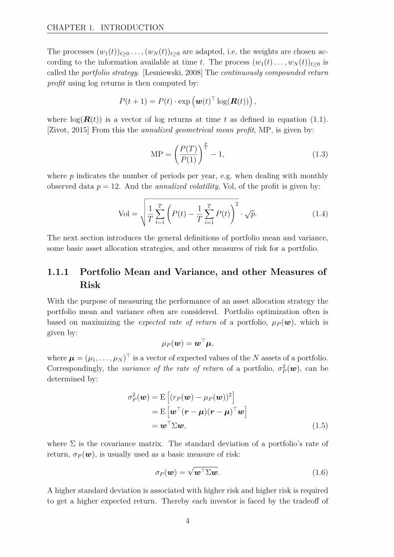
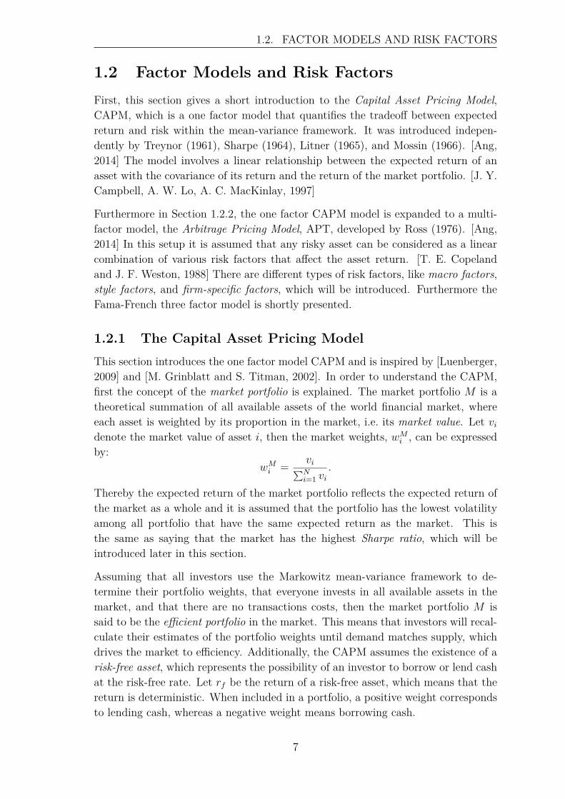
Now consider a mean-standard deviation diagram as shown in Figure 1.2, where eachpoint represents an asset with its expected rate of return µ and standard deviationσ. If one plots the market portfolio M in this diagram, then the efficient set ofportfolios consists of a straight line, called the capital market line, which starts in arisk-free point rf and passes through the market portfolio M .
µ
σ
rf
Capitalmarket line
M
Figure 1.2. Mean-standard deviation diagram with capital market line drawnfrom a risk-free point rf and passing through the market portfolioM . The points indicate assets with their expected rate of returnµ and standard deviation σ. The figure is inspired by [Luenberger,2009].
The capital market line describes the relation between the expected rate of return µof an asset and the risk of return, measured by σ. Let µM and σM be the expectedrate of return and standard deviation of the market rate of return described by themarket portfolio, and µP (w) and σP (w) be the expected rate of return and standarddeviation of an arbitrary efficient portfolio or asset. Then the capital market linedescribes a portfolio consisting of one risk-free asset rf and one efficient risky assetrM such that the expected rate of return of the portfolio is given by:
µP (w) = rf + µM − rfσM
σP (w). (1.11)
The numerator in the slope of the capital market line, µM−rf , is called risk premium,which is a kind of compensation for an investor that takes extra risk in holding a
8
1.2. FACTOR MODELS AND RISK FACTORS
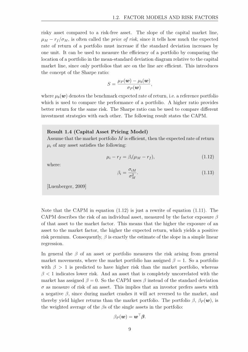
risky asset compared to a risk-free asset. The slope of the capital market line,µM − rf/σM , is often called the price of risk, since it tells how much the expectedrate of return of a portfolio must increase if the standard deviation increases byone unit. It can be used to measure the efficiency of a portfolio by comparing thelocation of a portfolio in the mean-standard deviation diagram relative to the capitalmarket line, since only portfolios that are on the line are efficient. This introducesthe concept of the Sharpe ratio:
S = µP (w)− µb(w)σP (w) ,
where µb(w) denotes the benchmark expected rate of return, i.e. a reference portfoliowhich is used to compare the performance of a portfolio. A higher ratio providesbetter return for the same risk. The Sharpe ratio can be used to compare differentinvestment strategies with each other. The following result states the CAPM.
Result 1.4 (Capital Asset Pricing Model)Assume that the market portfolioM is efficient, then the expected rate of returnµi of any asset satisfies the following:
µi − rf = βi(µM − rf ), (1.12)where:
βi = σiMσ2M
. (1.13)
[Luenberger, 2009]
Note that the CAPM in equation (1.12) is just a rewrite of equation (1.11). TheCAPM describes the risk of an individual asset, measured by the factor exposure βof that asset to the market factor. This means that the higher the exposure of anasset to the market factor, the higher the expected return, which yields a positiverisk premium. Consequently, β is exactly the estimate of the slope in a simple linearregression.
In general the β of an asset or portfolio measures the risk arising from generalmarket movements, where the market portfolio has assigned β = 1. So a portfoliowith β > 1 is predicted to have higher risk than the market portfolio, whereasβ < 1 indicates lower risk. And an asset that is completely uncorrelated with themarket has assigned β = 0. So the CAPM uses β instead of the standard deviationσ as measure of risk of an asset. This implies that an investor prefers assets witha negative β, since during market crashes it will act reversed to the market, andthereby yield higher returns than the market portfolio. The portfolio β, βP (w), isthe weighted average of the βs of the single assets in the portfolio:
βP (w) = w>β.
9
CHAPTER 1. INTRODUCTION
Inspired by the CAPM in equation (1.12) the random rate of return of asset i canbe written as:
ri = rf + βi(rM − rf ) + εi, (1.14)
where εi is the residual. From equation (1.12) it follows that E [εi] = 0. In addition,when taking the covariance of ri as given in equation (1.14) with the market rate ofreturn rM , it follows that Cov [εi, σM ] = 0. This implies that risk, measured by thevariance of an asset, σ2
i , can be decomposed into systematic risk and specific risk:
σ2i = β2
i σ2M + σ2
εi(1.15)
Total risk = systematic risk + specific risk,
where the systematic risk is the risk associated with the market as a whole.
Most investors want a high expected return and at the same time low risk. Thisintroduces the concept of diversification, which is a method to reduce the variance,as given in equation (1.15), by including additional assets in a portfolio. The riskassociated with the market, the systematic risk, cannot be reduced by diversification.Whereas specific risk can be diversified due to the uncorrelateness to the systematicrisk and the law of large numbers, by including a large number of assets in a portfolio.The following simple example shows how the variance of a portfolio behaves whenusing the Equally-Weighted strategy and a large number of assets in a portfolio.
Example 1 (Equally weighted portfolio)Consider an equally weighted portfolio, where wi = N−1. Then the variance of therate of return of the portfolio can be rewritten as:
σ2P (w) = N−2
N∑i=1
σ2i +N−2
6=∑i,j
σij (1.16)
= N−2Nσ2• +N−2N(N − 1)σ••
= N−1σ2• + N − 1
Nσ••
= N−1σ2•(1− ρ) + ρσ•.
The notation ∑6=i,j is a short form for ∑Ni=1
∑Nj=1,i 6=j. For a large number of assets N
it follows that:limN→∞
σ2P (w) = σ••.
Thus, the portfolio variance assymptotically is the average of the covariances be-tween the assets. Hence σ•• denotes the systematic risk that cannot be diversified,whereas N−1σ2
•(1−ρ) is the specific risk that can be diversified by including a largenumber of assets in a portfolio.Note that the correlation coefficient ρ has a lower bound, since it has to be ensured
10
1.2. FACTOR MODELS AND RISK FACTORS
that the portfolio variance σp(w) is positive semi-definite, i.e. σ2P (w) ≥ 0. Consider
the expression given in equation (1.16) and rewrite it:
σ2P (w) =N−2
N∑i=1
σ2i + ρ
6=∑i,j
σiσj
≥ 0
N∑i=1
σ2i ≥ −ρ
6=∑i,j
σiσj
ρ ≥ −∑Ni=1 σ
2i∑6=
i,j σiσj.
Considering the simplified case where all assets in a portfolio have variance σi = 1,it follows that:
ρ ≥ − N
N(N − 1) = −(N − 1)−1, (1.17)
which is the lower bound for ρ. 4
5 10 15 20
0.0
0.2
0.4
0.6
0.8
1.0
N
Por
tfolio
Var
ianc
e
ρ = − 0.3ρ = 0ρ = 0.3
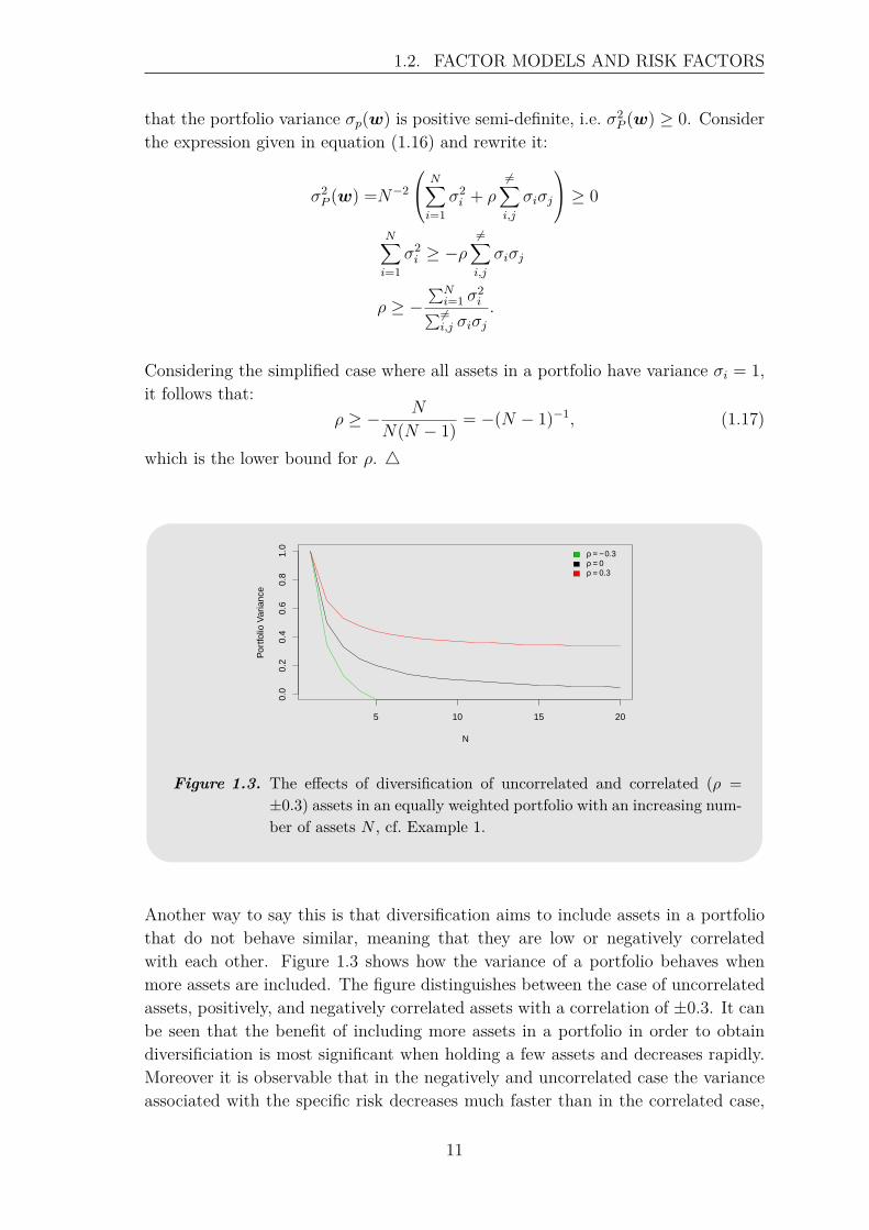
Figure 1.3. The effects of diversification of uncorrelated and correlated (ρ =±0.3) assets in an equally weighted portfolio with an increasing num-ber of assets N , cf. Example 1.
Another way to say this is that diversification aims to include assets in a portfoliothat do not behave similar, meaning that they are low or negatively correlatedwith each other. Figure 1.3 shows how the variance of a portfolio behaves whenmore assets are included. The figure distinguishes between the case of uncorrelatedassets, positively, and negatively correlated assets with a correlation of ±0.3. It canbe seen that the benefit of including more assets in a portfolio in order to obtaindiversificiation is most significant when holding a few assets and decreases rapidly.Moreover it is observable that in the negatively and uncorrelated case the varianceassociated with the specific risk decreases much faster than in the correlated case,
11
CHAPTER 1. INTRODUCTION
which confirms the concept of diversification. Note that as shown in Example 1there is a lower bound for the correlation coefficent ρ that ensures that the portfoliovariance does not get negative.
Since equation (1.14) can be considered as a simple linear regression, one can mea-sure the fraction of systematic risk in the variance of the return of the ith asset in aportfolio using the R2 statistic, which describes the percentage of the total variationin the rate of return that is explained by the regression equation, i.e.:
R2 =σ2i − σ2
εi
σ2P (w) ,
where σ2i is the variance of the ith asset, σ2
εithe variance of the residual of the ith
asset, and σ2P (w) is the portfolio variance. A high R2 indicates that the variance
consists of mostly systematic risk, whereas a low R2 indicates mostly specific risk.
The concept of diversification is connected with the CAPM by the β of an asset,since it can be rewritten as:
β = ρiMσiσM
,
where ρiM is the correlation between the return of asset i and the market return.So a high β means low diversification benefits. As mentioned earlier, investors wantto hold assets with low or negative β such that when the market crashes, they holdassets that do not crash.
One of the drawbacks of the CAPM is that it focuses on the variance and covariancesof the asset returns as measure of risk. The variance is a first-moment measure ofrisk, but most investors also consider higher moment measures of risk, e.g. kurtosisand skewness of asset returns. So indeed including additional assets in a portfolioreduces the variance, but other measures of risk may not be diminished. A portfoliocan get more negatively skewed thus it has a higher downside risk, which would notbe detected by the variance or β of an asset.
The CAPM has some very strong assumptions, which often are not met in reality.For instance the CAPM assumes that investors have mean-variance utility, but inreality investors have much more complicated utilities. In addition, it is assumedthat investors have homogeneous expectations, although they are heterogeneous.And it is disregarding transaction costs, which can vary across assets. Furthermore,the CAPM is a single-period model, which assumes that returns are independentlyand identically distributed and that they are jointly multivariate normal. [J. Y.Campbell, A. W. Lo, A. C. MacKinlay, 1997]
As mentioned earlier, the market portfolio reflects systematic risk, which effects allassets. The next section extends the model setup to also include style factors likevalue-growth investing and momentum, or macro factors like inflation and economicgrowth, that have risk premia based on, e.g. investor characteristics and productioncapabilities of the economy.
12
1.2. FACTOR MODELS AND RISK FACTORS
1.2.2 Multifactor Models and the Arbitrage PricingTheory
Unless otherwise stated, this section is based on [T. E. Copeland and J. F. Weston,1988], [Overby, 2010], and [Ang, 2014]. The previous section introduced the CAPM,which assumes that there is only one factor in the market, namely the market factor.This section aims to generalize this setup to multifactor models, that describe theunderlying drivers of assets by several factors.
One of the first models that used multiple factors was the Arbitrage Pricing Theory,APT, which has less restrictions regarding the assumptions made in the CAPM suchas assumptions on the distribution of the returns or the utility function of investors.Moreover it does not require to identify the market portfolio, which can be difficult.The APT is mainly based on the assumption of no arbitrage i.e. the factors cannotbe diversified away.
It is assumed that the rate of return, r, of the assets can be modelled as a linearfunction of K unknown factors, f , using a multifactor model:
r = µ+Bf + ε (1.18)E [f ] = 0E [ε|f ] = 0
E[εε>
]= Σε,
where µ is the intercept of the factor model, B = [β1, . . . ,βN ]> is the matrix offactor loadings, and ε is the residual that describes the specific risk. [J. Y. Campbell,A. W. Lo, A. C. MacKinlay, 1997] It is assumed that the factors f only account forcommon variation, systematic risk, in the asset returns. Note that returns that havesimilar factor loadings on specific factors are likely to be correlated. The expectedreturn of the assets is given by:
E [r] = E [µ+Bf + ε] = E [µ] +BE [f ] + E [ε] = µ.
By assuming independence of the residuals, the law of large numbers says that ina portfolio consisting of a large number of assets the specific risk vanishes. Conse-quently, the overall rate of return of a portfolio, rP (w), can be expressed as:
rP (w) = w>r = w>µ+w>Bf , (1.19)
where it is assumed that wi ≈ N−1, i.e. no asset is overweighted, and ∑Ni=1wiβij =
βPj = 0 for each factor fj where j = 1, . . . , k. The second assumption ensuresthat there is no exact collinearity between the risk factors and thereby the overallmodel is factor neutral. This implies that w>B = 0>, i.e. w ∈ Null(B). Dueto this assumptions, the portfolio given in equation (1.19) is called an arbitrageportfolio, since both systematic and specific risk are eliminated, and therefore it canbe rewritten as:
rP (w) = w>µ = µP (w) = 0. (1.20)
13
CHAPTER 1. INTRODUCTION
The return rP (w) in equation (1.20) has to be equal to zero for otherwise it wouldbe possible to attain an infinite return without risk and capital requirements. Theresult from equation (1.20) together with w>B = 0> imply that the expectedreturn µ must be a linear combination of a constant vector λ = (λ1, . . . , λk) andthe coefficient matrix of factor loadings B = [β1, . . . ,βN ]>, i.e. it is assumed that:
E [r] = µ ≈ 1λ0 +Bλ, (1.21)
where λ0, . . . , λk are risk premia. If there exists a risk-free asset with return rf thenλ0 = rf . Hence equation (1.21) can be rewritten as:
µ− 1rf = Bλ.
Assuming that λ = δ − 1rf this can be formulated as:
µ− 1rf = B(δ − 1rf ), (1.22)
where δ is the expected rate of return on a portfolio with unit loading to the jthfactor and zero loading on all other factors. Such a portfolio is called a pure factorportfolio. The formulation of λ = δ − 1rf is equivalent to the risk premium for-mulation in the CAPM in equation (1.12) with the difference that the CAPM onlyconsiders the market factor whereas the APT considers multiple factors.
Interpreting equation (1.22) as a linear regression equation and assuming that re-turns are jointly normal distributed and that the factors δ are linearly transformedto be orthonormal, the elements βij of the matrix B are defined in a similar mannerto the CAPM as stated in equation (1.13), this is:
βij =Cov
[µi, δj
]Var
[δj] .
So the CAPM can be viewed as a special case of the APT.
Let r(l)P (w) denote the return of the lth factor portfolio, where l = 1, . . . , k, which
can be expressed by:
r(l)P (w) = µ
(l)P (w) +
k∑j=1
β(l)Pj(w)fj,
where:
µ(l)Pj(w) =
N∑i=1
w(l)i µi,
β(l)Pj(w) =
N∑i=1
w(l)i βij for β
(l)Pj(w) =
1 if j = l,
0 if j 6= l,(1.23)
N∑i=1
w(l)i = 1.
14
1.2. FACTOR MODELS AND RISK FACTORS
In matrix notation equation (1.23) can be expressed as WB = Ik, where W is aN × k matrix of weights, B is a k × k matrix of factor loadings, and Ik is a k × kidentity matrix. Note that there has to be solved a system of linear equations.Hence it is ensured that there are unique solutions if there are the same number ofequations as there are unknowns. Else if there are fewer equations than unknowns,there are infinitely many solutions. The risk premium for the lth factor is thendefined by:
λl = µ(l)P (w)− rf .
Using this setup, Ross (1976) has shown that in the absence of arbitrage opportu-nities the APT can be formulated as:
Result 1.5 (Abitrage Pricing Theory)Consider an investment without specific risk, then the expected rate of returnis given by:
µ ≈ 1λ0 +Bλ,
where λ0 is the intercept and λ = (λ1, . . . , λk)> are risk premia for the Kfactors. [J. Y. Campbell, A. W. Lo, A. C. MacKinlay, 1997]
The disadvantage of multifactor models is that they do neither specify the numberfactors nor identify their meaning. As mentioned in [Ang, 2014] risk factors are likenutrients are to food. Such as some types of food are a bundle of nutrients andothers contain only one nutrient, assets can consist of one or more risk factors. Theintuition behind this is, that the risk factors behind the assets matter, not the assetsthemselves.
It can be distinguished between macro factors that are common for several assets ina portfolio due to the presence of, e.g. inflation or volatility, in the financial marketand style factors like value-growth or size based on firm-characteristics, which willbe explained later in this section. These two types of factors are undiversifiable.Specific factors, that for instance only affect a specific firm, can be diversified by in-cluding a large number of assets as explained above. Depending on the exposure andtype of the underlying, undiversifiable risk factors assets have different risk premia.These premia compensate for low returns during bad times with a premium of highreturns in the long run. This means that different risk premia describe different setsof bad times, i.e. bad economical times. Every investor has an individual definitionof ’bad time’, which among others depends on the investor’s income, liabilites, andrisk aversion. Depending on the aggregate supply of a factor in the financial marketsand type of risk factor, risk premia can be positive, negative, or zero. Assets thathave high returns during bad times, e.g. are negatively correlated to market move-ments, have a high price and thereby a low risk premium. In contrast have assets
15
CHAPTER 1. INTRODUCTION
that are positively correlated with market movements, i.e. crash together with mostother assets, a low price and high risk premium to compensate for these losses.
There exists a plenty of different factors, where the most fundamental factor is themarket factor described by the CAPM as introduced in the previous section. But inorder to use them, one should justify the academic research behind them and theyshould satisfy the following which is inspired by [Mesomeris, 2013]:
• Risk factors shall be explainable.• They must be persistent, i.e. continue to exist and not just be a phenomenon
for a short time period.• In isoloation they should have attractive return characteristics.• A risk factor should have low correlation to traditional market β’s and other
risk factors considered for a portfolio.• The risk factor must be accessible.• Risk factors should be priced.
The following gives a short explaination of macro and style factors.
Macro Factors
Macro factors affect all investors and prices of assets in an economy. For instanceaffects low growth and high inflation everyone, but to different degree. Many macrofactors are lasting, e.g. when inflation is low today, it is likely that it will be lownext month. One other well-known macro factor is volatility, since stock returnsare negatively correlated to volatility, which is also known as the leverage effect.This effect describes the relationship between stock returns and volatilities, sincestock prices fall when volatility increases. Volatility can also be viewed as a kind ofuncertainty risk factor, since it is highly correlated with the uncertainty of investorsto e.g. policy decisions that can affect the economy. There are many other macrofactors, e.g. economic growth, interest rate risk, or currency risk.
The following section introduces some of the style factors considered in this thesis.
Style Factors
As mentioned earlier, the assumptions of the CAPM model, introduced in Section1.2.1, do often not hold in reality. The model has been tested extensively in the1970s using time series regressions of e.g. the returns of the S&P 500.1 The testsshowed that the assumption of the CAPM that the market factor is the only factorin the market were not satisfied, hence there must be other factors in the marketthat influcence asset prices. [M. Grinblatt and S. Titman, 2002] This has motivatedto introduce models which are based on several factors.
1The Standard and Poor’s S&P 500 stock market index includes the 500 leading companies inthe US. [SP Dow Jones Indices, 2015]
16
1.2. FACTOR MODELS AND RISK FACTORS
Fama and French (1993) introduced a model that explains assets by three factors.The first factor is the traditional market factor M from the CAPM, and then theyhad two additional factors to capture a size factor, S, and a value-growth factor, V :
µi = rf + βi,ME [rM − rf ] + βi,SE [S] + βi,VE [V ] .
The following explains the size and value-growth factors.
Size FactorThis factor describes the market capitalization of stocks. It has been observed thatsmall firms outperform large firms. The effect was discovered in 1981, but since themid-1980s the existence of this effect is debatable. There are made many studiesthat argue for the disappearance of the effect, and others can find the effect forspecial segments. For are discussion of the disappearance of the size effect see e.g.[Crain, 2011].
Value-growth FactorStocks that have a low price in relation to their net worth, which is the same as ahigh book-to-market ratio, are called value stocks. The book-to-market ratio is thebook value divided by the market capitalization. This are companies that currentlyare out of favour in the financial market or newer companies with unknown trackrecords. [J. O. Reilly, S. O. Barba, N. Pavlov, 2003] On the other hand, stocks withlow book-to-market ratios are called growth stocks. This are typically companiesthat had good earnings in the recent years and are expected to continue to yieldhigh profit growth. The investment strategy of going long value stocks and shortgrowth stocks is known as the Value-Growth strategy. The reason for this is thatvalue stocks outperform growth stocks, on average. It has been a robust premiumfor many years.
The factors in the Fama-French model can be constructed by using characteristic-sorted portfolios, which means that the factors are estimated by using portfolios thatare formed based on firm characteristics as described for the different style factors.[M. Grinblatt and S. Titman, 2002] Besides the size and value-growth effects thereare other effects, as will be explained in the following.
Momentum FactorMomentum describes the strategy of buying stocks that have increasing returns overthe past months and selling stocks with the lowest returns over the same period.The effect is that winner stocks continue to win and losers continue to lose. It isobserved that the Momentum strategy yields higher profits than the Value-Growthand Size strategies do, and it is observable in every asset class. The effect can beadded to the Fama-French model, where positive momentum βs indicate winnerstocks and negative βs indicate loser stocks.
Low Risk FactorDescribes assets that have low volatility and is often called Low Volatility strategy.2
2Source: Internal documentation from Jyske Bank A/S.
17
CHAPTER 1. INTRODUCTION
Quality FactorQuality describes the effect of firms facing negative returns in future earnings an-nouncements, when a large proportion of their earnings come from revenue, com-pared to firms where earnings are based on cash flow.2
Strategies like Size, Value-Growth, and Momentum are called cross sectional strate-gies, since they compare one group of stocks with another group, e.g. value stockswith growth stocks. It should be noted that both the CAPM, APT, and Fama-French model assume that the βs are constant, but the exposure of assets to sys-tematic factors vary over time, and often increases during bad times.
This chapter introduced some basic economical concepts regarding portfolio opti-mization including different measures of risk and some traditional asset allocationstrategies. Furthermore, some important economical models for factor models havebeen introduced in order to get a better understanding of diversification and riskfactors. In order to establish risk-based asset allocation strategies in Chapter 3, thenext chapter introduces statistical methods to find underlying, lower dimensionalfactors. These are the projection methods principal component analysis, PCA, andfunctionional principal component analysis, fPCA.
18
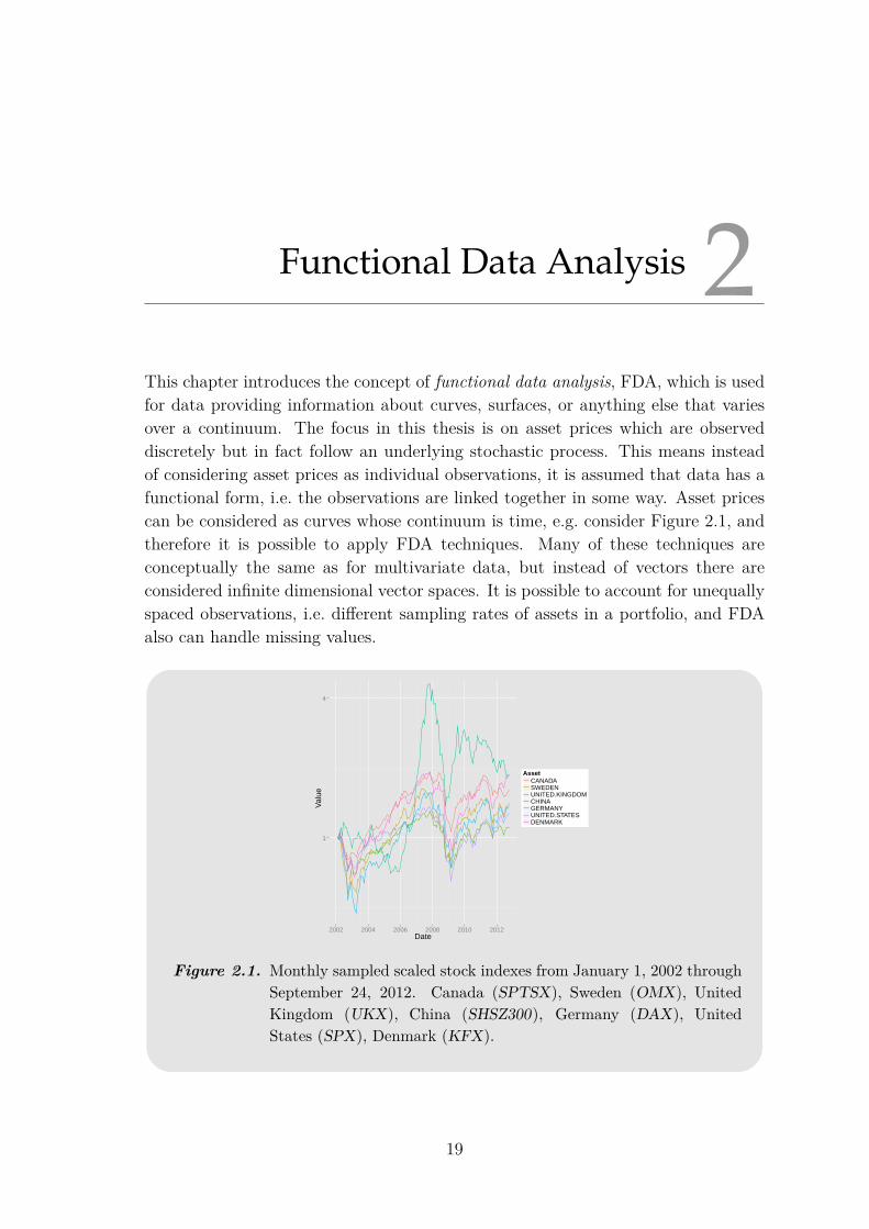
Functional Data Analysis 2This chapter introduces the concept of functional data analysis, FDA, which is usedfor data providing information about curves, surfaces, or anything else that variesover a continuum. The focus in this thesis is on asset prices which are observeddiscretely but in fact follow an underlying stochastic process. This means insteadof considering asset prices as individual observations, it is assumed that data has afunctional form, i.e. the observations are linked together in some way. Asset pricescan be considered as curves whose continuum is time, e.g. consider Figure 2.1, andtherefore it is possible to apply FDA techniques. Many of these techniques areconceptually the same as for multivariate data, but instead of vectors there areconsidered infinite dimensional vector spaces. It is possible to account for unequallyspaced observations, i.e. different sampling rates of assets in a portfolio, and FDAalso can handle missing values.
1
4
2002 2004 2006 2008 2010 2012Date
Val
ue
AssetCANADASWEDENUNITED.KINGDOMCHINAGERMANYUNITED.STATESDENMARK
Index − Portfolio Components
Figure 2.1. Monthly sampled scaled stock indexes from January 1, 2002 throughSeptember 24, 2012. Canada (SPTSX), Sweden (OMX), UnitedKingdom (UKX), China (SHSZ300), Germany (DAX), UnitedStates (SPX), Denmark (KFX).
19
CHAPTER 2. FUNCTIONAL DATA ANALYSIS
Moreover, in order to extract risk factors that lie behind the assets of a portfolio,principal component analysis, PCA, is introduced in Section 2.2 and expanded tofunctional principal component analysis, fPCA, considering data to be functionalinstead of multivariate in Section 2.3. The motivation for this is that fPCA isbetter to capture the variability of the asset returns, which is essential for the assetallocation strategies introduced in Chapter 3. This is due to the fact that in fPCAit is possible to observe the behaviour of the eigenfunctions over time in contrast toPCA that just gives a static, non-temporal estimate of the eigenvectors. In addition,functional data is smoothed before performing a fPCA, which improves the signal-to-noise ratio of data and therefore may improve the allocation strategies by specifyingthe true underlying risk factors.
The following sections give an introduction to FDA, the concept of basis functions,and of smoothing functional data. Furthermore the projection methods PCA andfPCA are introduced, and some important results for these methods are shown.
2.1 Functional DataThis section is based on [J. O. Ramsay , B. W. Silverman, 2005] and [Zhang, 2014].In functional data analysis, observed data functions are considered to provide in-formation about possible infinite-dimensional curves. The observations often havetime as continuum, but could also have other continua such as spatial position.
The reason that functional data is not considered as multivariate data is the as-sumption of the observations being linked together in some way, meaning that datahas a functional form. Consider the observed data (tj, yj) for j = 1, . . . , n where yjis a response observed at times tj. The transformation to the functional form hastwo cases; the discrete values are assumed to be errorless:
y(tj) = yj = x(tj),
where x(tj) is a smooth function. This process of converting discrete data intofunctional data is called interpolation. The other case is given by:
y(tj) = yj(t) = x(tj) + εj. (2.1)
The second case may involve smoothing of data in order to reduce the residual εj.One possible smoothing technique will be introduced in Section 2.1.2. Equation(2.1) can be rewritten to represent all N curves:
yi(tj) = xi(tj) + εi(tj) for i = 1, . . . , N and j = 1, . . . , ni. (2.2)
It is assumed that the function xi(t) can be decomposed into:
x(t) + νi(t),
20
2.1. FUNCTIONAL DATA
where x(t) is the mean function, which is given by:
x(t) = N−1N∑i=1
xi(t), (2.3)
and νi(t) is the ith individual variation from x(t) with ∑Ni=1 vi(t) = 0. Thus a func-
tional data set is modelled as independent realizations of an underlying stochasticprocess:
yi(tj) = x(tj) + νi(tj) + εi(tj),
where it is assumed that νi(t) and εi(t) are independent. Moreover it is assumedthat νi(t) and εi(t) follow stochastic processes:
νi(t) ∼ SP(0, v) and εi(t) ∼ SP(0, vε),
where SP(x, v) denotes a stochastic process with mean function x(t) and covariancefunction v(s, t), which is given by:
v(s, t) = (N − 1)−1N∑i=1
(xi(s)− x(s)) (xi(t)− x(t)) . (2.4)
Moreover it is assumed that vε(s, t) = σ2(t)1[s = t], where σ2(t) is the residualvariance function that measures the variation of the measurement errors.
Normally the data transfromation takes place seperately for each curve i, but ifthere is a low signal-to-noise ratio or sparsely sampled data, it can be useful totake information from neighboring or similiar curves into account to get more stableestimates for a curve.
The assumption of a smooth function usually means that the function x(t) has one ormore derivatives. Thereby functional data analysis uses information in the featuresof a curve, i.e. slopes, curvature, crossings, peaks, or valleys. Functional featurescan be considered as events that are related to a specific value of the argumentt. They can be characterized by their location, amplitude, or width, which can betreated as a measure of dimension. For instance, a peak can be considered as beingthree-dimensional, since location, amplitude, and width have to be known for fullinformation of the peak.
The argument values t1, . . . , tnican be the same for all curves i, but can also vary
from curve to curve. In addition, it is also possible to deal with curves that havemissing values, since data is transformed to a continuous structure. It is also im-portant to consider the sampling rate of data, which takes into account the ratiobetween the argument values tj relative to the amount of curvature, which is mea-sured by the second order derivative |D2x(t)| or [D2x(t)]2. The higher the curvatureis, the more points are needed for a good estimation of a curve. [J. O. Ramsay , B.W. Silverman, 2005]
In order to represent the continuous functions, the next section introduces the con-cept of basis functions.
21
CHAPTER 2. FUNCTIONAL DATA ANALYSIS
2.1.1 Basis FunctionsThis section is based on [J. O. Ramsay , B. W. Silverman, 2005]. In functionalspace basis functions are the counterpart to basis vectors in vector space. Thismeans, that such as every vector can be represented by a linear combination ofbasis vectors, every continuous function can be represented by a linear combinationof basis functions.
Consider the vector-valued function x with components x1(t), . . . , xN(t). Moreoverlet φ be the vector-valued function with K independent, real-valued basis functioncomponents φ1(t), . . . , φk(t), and let C be a N × K coefficient matrix, then thesimultaneous expansion of all N curves can be expressed by:
x = Cφ(t). (2.5)
For a single curve xi(t) this corresponds to:
xi(t) = c>i φ(t) = φ(t)>ci.
This shows, that basis expansion methods represent possibly infinite functions byfinite dimensional vectors.
The number of basis functions K can be seen as a parameter, that is selectedaccording to characteristics in data, often by using a cross validation method. Itis preferred to have a low value of K in order to avoid overfitting and to reducecomputations. The case K = ni, where ni is the number of observations of curve i,is known as exact representation or interpolation.
Basis functions φk are said to be orthogonal over some interval t ∈ T if for all m:
∫Tφk(t)φm(t) =
0 k 6= m,
λm k = m,(2.6)
where λm ∈ R and if λm = 1, then the basis functions are said to be orthonor-mal. There are different choices of basis functions depending on the structure ofdata. The most common basis functions are Fourier- , B-splines- , monomials- ,and wavelets basis functions. When dealing with periodic data the most widelyused basis functions are Fourier functions, whereas in the non-periodic case it isB-splines. [J. O. Ramsay , B. W. Silverman, 2005] In the following B-splines will beintroduced.
B-Splines
Spline functions have replaced polynomials, since they have the property of fastcomputation and a high degree of flexibility. [J. O. Ramsay , B. W. Silverman,2005] In order to define a spline, consider the interval over which a function is tobe approximated. The interval is divided into L subintervals, which are seperatedby so-called breakpoints τl , l = 1, . . . , L − 1, i.e. an interval [a, b] is diveded into
22
2.1. FUNCTIONAL DATA
a = τ0 < τ1 < · · · < τL−1 < τL = b. The breakpoints τl for l = 1, . . . , L − 1 arecalled the interior breakpoints. Over each subinterval [τr, τr+1) for r = 0, . . . , L− 1,a spline is a polynomial of order m, which are required to join smoothly at theinterior breakpoints. This means that the derivatives match up to the order one lessthan the degree of the polynomial.
The first polynomial has m degrees of freedom, but each subsequent polynomial hasonly one degree of freedom because of the m− 1 constraints on its behaviour. Thisimplies that the total number of degrees of freedom in the fit equals the order of thepolynomials plus the number of interior breakpoints, L+m degrees of freedom.
The higher the order, the better is the approximation of the function. In addition,greater flexibility in a spline is achieved by increasing the number of breakpoints.The breakpoints do not have to be equally spaced, so it is preferable to have morebreakpoints where the function posses the most variation. Note that given an orderm and a breakpoint sequence τ , every basis function φk is itself a spline function.And that any linear combination of basis functions φk is a spline function.
A B-spline basis function of order m has the compact support property. The supportof a function is the set of points where the function is not zero-valued, if the functionis positive over no more thanm intervals, and when these are neighbouring intervals.This property is important for fast computation, since it implies that when there areK B-spline basis functions, the order K matrix of inner products of these functionswill be band-structured, with m − 1 subdiagonals above and below the diagonalcontaining nonzero values. So the computation of spline functions increases onlylinearly with K.
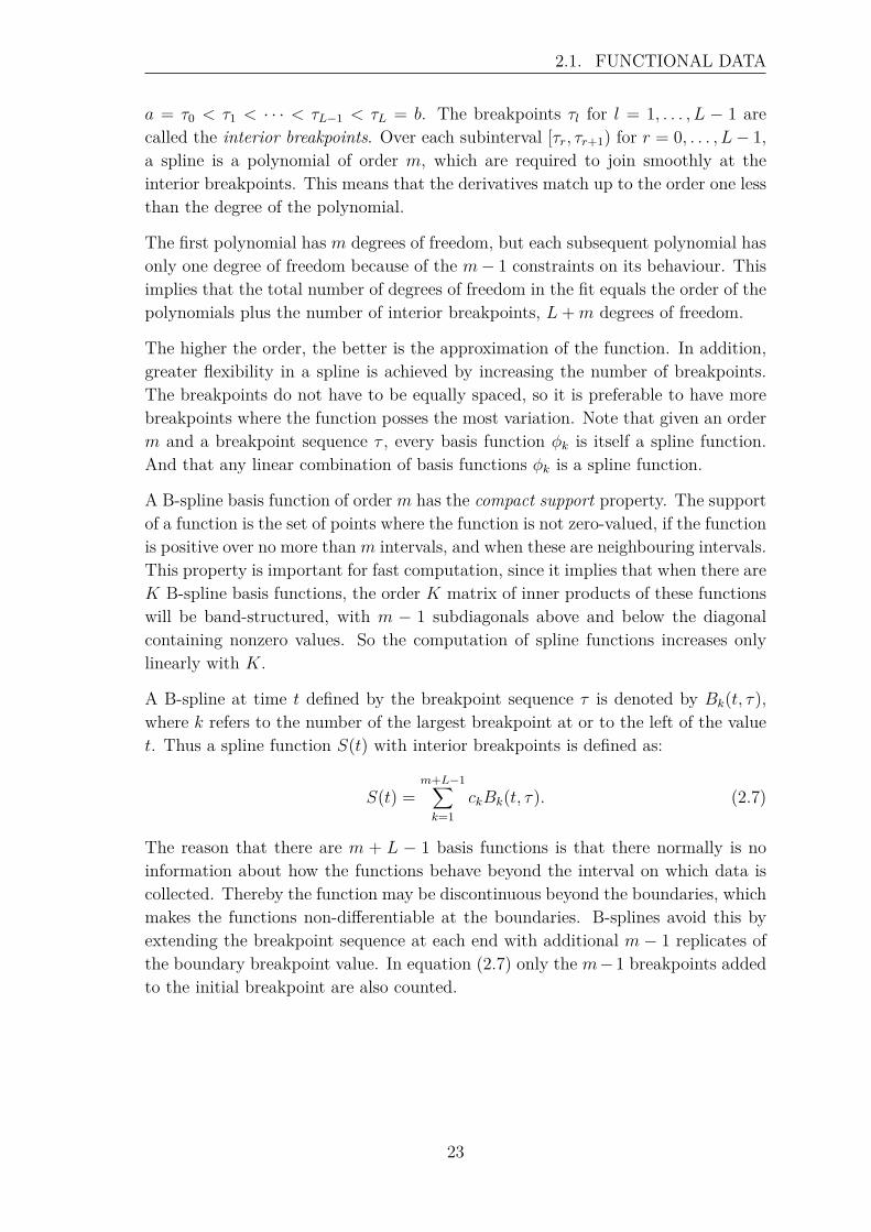
A B-spline at time t defined by the breakpoint sequence τ is denoted by Bk(t, τ),where k refers to the number of the largest breakpoint at or to the left of the valuet. Thus a spline function S(t) with interior breakpoints is defined as:
S(t) =m+L−1∑k=1
ckBk(t, τ). (2.7)
The reason that there are m + L − 1 basis functions is that there normally is noinformation about how the functions behave beyond the interval on which data iscollected. Thereby the function may be discontinuous beyond the boundaries, whichmakes the functions non-differentiable at the boundaries. B-splines avoid this byextending the breakpoint sequence at each end with additional m− 1 replicates ofthe boundary breakpoint value. In equation (2.7) only the m−1 breakpoints addedto the initial breakpoint are also counted.
23
CHAPTER 2. FUNCTIONAL DATA ANALYSIS
0 100 200 300
0.0
0.4
0.8
Figure 2.2. B-spline basis with K = 30 basis functions.
The position of the interior breakpoints τl can be determined by different methods.Often the default method is equal spacing, which is good as long data has a constantsampling rate as mentioned in Section 2.1. An example of an equally spaced B-splinebasis with 30 breakpoints can be seen in Figure 2.2. Another possibility is to place abreakpoint at every j’th breakpoint, where j is a fixed number selected in advance.There exists algorithms for breakpoint positioning which are similar to variableselection techniques in multivariate regression. [J. O. Ramsay , B. W. Silverman,2005]
One possible approach of constructing orthogonal basis functions is functinal prin-cipal component analysis, fPCA, which will be introduced in Section 2.3. But firstthe following section explains how data can be smoothed using a roughness penalty.
2.1.2 Smoothing Functional DataThis section is inspired by [J. O. Ramsay , B. W. Silverman, 2005] and [J. O.Ramsay, G. Hooker, S. Gaves, 2009]. When data observations may contain errors,data it has to be smoothed in order to obtain a functional form as stated in Section2.1. There are different techniques available, but the focus here is on smoothingdata using a roughness penalty. This method is based on weighted least squares,which is given by:
SMSSE(y|c) = (y − Φ(t)c)>W (y − Φ(t)c),
where W is a symmetric positive definite weight matrix , y is a response vector,c is a vector of coefficients, and Φ(t) is a matrix consisting of basis functions asdescribed in Section 2.1.1. The basis functions in Φ could for instance be B-splines.
When the covariance matrix Σe for the resiuduals εj is known, then the weightmatrix is given by:
W = Σ−1e .
To be able to establish smoothing by a roughness penalty, one has to quantify thenotion of roughnesss of a function. A natural measure could be the integrated
24
2.1. FUNCTIONAL DATA
squared mth derivative:PENL(x) =
∫[Lx(s)]2 ds,
where L = Dm is the mth derivative. A rough function has high curvature, whichyields high values for PENL(x). Let x(t) be the vector resulting from a functionx evaluated at time arguments t. Then the penalized residual sum of squares isdefined by:
PENSSEλ(x|y) = (y − x(t))>W (y − x(t)) + λPENL(x), (2.8)
where λ ≥ 0 is a smoothing parameter that measures the tradeoff between goodnessof fit of data and the variability of the function x. When λ = 0 then the penalityterm has no influence and equation (2.8) is a usual weighted least squares problem.As λ→∞ the penalty term gets more influence so curvature is more penalized. Inthe field of statistics this is also known as ridge regression.
In order to obtain a smoothed functional data set, the aim is to minimize equation(2.8). Substituting the basis expansion x(t) = c>Φ(t) = Φ>(t)c into this equation,yields:
PENSSEλ(x|y) = (y − c>Φ(t))>W (y − c>Φ(t)) + λc>Rc, (2.9)
which follows from the following computation:
PENL(x) =∫
[Lx(s)]2 ds
=∫ [
Lc>Φ(s)]2ds
=∫c>LΦ(s)LΦ(s)>c ds
= c>∫LΦ(s)LΦ(s)>ds c
= c>Rc,
where R =∫LΦ(s)LΦ(s)ds is the roughness penalty matrix. It is possible to ob-
tain analytic solutions for some types of basis systems, e.g. for the B-spline basis,but the details for this computation are complicated and omitted in this thesis.Differentiating equation (2.9) with respect to c yields:
−2Φ(t)>Wy + Φ(t)>WΦ(t)c+ λRc = 0.
Hence the estimated coefficient vector is given by:
c =(Φ(t)>WΦ(t) + λR
)−1Φ(t)>Wy, (2.10)
which is exactly the ridge regression estimate.
In order to determine λ, generalized cross validation, GCV, with the following crossvalidation statistic as criterium is used:
GCV(λ) = n−1SMSSE(n−1trace(I −H))2 , (2.11)
25
CHAPTER 2. FUNCTIONAL DATA ANALYSIS
which was developed by Craven and Wahba (1979), see [Craven and Wahba, 1979].It is an approximation to the statistic obtained by leave-one-out cross validation,LOOCV, when using a linear regression model which is given by:
LOOCV = n−1n∑i=1
(SMSSE1− hi
)2
.
This result can for instance be found in [Hyndman, 2014]. LOOCV is a crossvalidation method where all observations expect from one are used as trainingsset and the excluded observation is used as validation set, which is done until allobservations have been in the validation set. [J. Friedman, T. Hastie, R. Tibshirani,2009] When using cross validation to find the smoothing parameter λ one has to payattention when choosing possible λ values to be validated, since the linear systemto be solved has limitations. Define the term in the parenthesis in equation (2.10)as:
M(λ) = Φ(t)>WΦ(t) + λR.
The matrices Φ(t)>WΦ(t) and R have elements of completely different size, butM(λ) has to be invertible in equation (2.10), which poses some limitations. [J. O.Ramsay , B. W. Silverman, 2005] suggests that the size of λR should not exceed1010 times the size of Φ(t)>WΦ(t).
It is possible to make λ dimensionless by considering log10(λ), which is in accordancewith the fact that λ > 0 when there is imposed a penality. So the roughness penaltyPENL(x) should be multiplied by 10ν , where ν = log10(λ).
Before introducing fPCA in Section 2.3, the basic ideas of PCA for multivariatedata are explained in the next section.
2.2 Principal Component AnalysisThis section is inspired by [Tvedebrink, 2014] and [J. O. Ramsay , B. W. Silverman,2005]. PCA is a dimensionality reduction method that uses orthogonal transfor-mations to transform a set of variables into a set of linearly uncorrelated variablesknown as principal components. The method is defined in such a way that the firstprincipal component accounts for the largest possible variance in data, and eachsubsequent component has the highest possible variance subject to the constraintof being orthogonal to the preceding components. The method is often confusedwith factor analysis, which is a very similar method but assumes that variables canbe expressed as a linear combination of underlying factors. Hence factor analysisassumes that there exist underlying factors, whereas PCA just is a dimensionalityreduction method.
In the case of multivariate data a matrix X is considered. Without loss of generality,it is assumed that the matrix is centered, which means that X = X − N−111>X,where N is the number of observations in data.
26
2.2. PRINCIPAL COMPONENT ANALYSIS
In addition, the covariance matrix V can be expressed by:
V = N−1X>X, (2.12)
which is of dimension p × p. It is possible to look at a linear combination of thevariable values:
fi =p∑j=1
βjxij = β>xi, i = 1, . . . , N, (2.13)
where β is a weighting vector (β1, . . . , βp)> and xi is an observed vector (xi1, . . . , xip)>.PCA is then used to define sets of normalized weights that maximize variation in thefi’s. The first step is to find a vector ξ1 = (ξ11, . . . , ξp1)> such that the covariance:
Cov [Xξ1] = E[(Xξ1)>Xξ1
]− E [Xξ1]> E [Xξ1]
= E[ξ>1 X
>Xξ1]− ξ>1 E [X]> E [X] ξ1
= ξ>1 Cov [X] ξ1 = ξ>1 V ξ1, (2.14)
is as large as possible. To ensure that the covariance not gets arbitrarily large, thefollowing constraint is introduced:
‖ξ1‖2 = ξ>1 ξ1 = 1.
The problem can also be formulated as maximizing the mean square:
1N
N∑i=1
f 2i1 subject to ‖ξ1‖2 = 1,
where fi1 = ∑pj=1 ξj1xij = ξ1xi. The linear combination fi1 is also called a principal
component score. Moreover, the subsequent projections have to be uncorrelated tothe previous ones:
p∑j=1
ξjkξjl = ξ>k ξl = 0, k < m ≤ p,
where m indicates the number of steps taken, which are limited by the number ofvariables p.
This means that the projections are orthogonal to each other, which guaranteesthat they are describing a new underlying feature in data. Based on the introducedconstraints, the following maximization problem can be formulated:
maxξ1ξ>1 V ξ1 − λ(ξ>1 ξ1 − 1), (2.15)
which is solved by:
(V − λI)ξ1 = 0V ξ1 = λξ1. (2.16)
This can be considered as finding the eigenvalues λ and eigenvectors ξj of the co-variance matrix V . An eigenvector can represent the direction of a component and
27
CHAPTER 2. FUNCTIONAL DATA ANALYSIS
the corresponding eigenvalue can represent how much variance there is in data inthis direction.
Since the covariance matrix V is positive semi-definite, it can be decomposed intoan orthogonal matrix U and a diagonal matrix Λ, whose entries are the eigenvaluesλ1 > · · · > λp. The decomposition is then given by:
V = U>ΛU =p∑j=1
λjuju>j . (2.17)
Using this expression in equation (2.15) and defining ξ1 = Uξ1, where:∥∥∥ξ1
∥∥∥2= ξ>1 ξ1 = (Uξ1)>Uξ1 = ξ>1 U
>Uξ1 = ξ>1 ξ1 = ‖ξ1‖2 ,
the maximization problem from equation (2.15) can be rewritten as:
maxξ1:ξ>
1 ξ1=1ξ>1 Λξ1 = max
ξ1:ξ>1 ξ1=1
p∑j=1
ξ21jλj.
This is maximal when ξ11 = 1, so ξ1 = e1, where e1 is the unit vector with a one inthe first entry. As mentioned, the next component has to be uncorrelated with thefirst component, so:
0 = Cov [Xξ1, Xξ2] = ξ>1 Cov [X,X] ξ2 = ξ>1 U>ΛUξ2 = ξ>1 Λξ2. (2.18)
Since ξ1 = e1, equation (2.18) reduces to 0 = λ1ξ21 ⇔ ξ21 = 0. Hence, the newmaximization problem is:
maxξ2:ξ>
2 ξ2=1;ξ21=0ξ>2 Λξ2 = max
ξ2:ξ>2 ξ2=1;ξ21=0
N∑j=1
ξ22jλj,
which implies that ξ22 = 1, so ξ2 = e2, where e2 denotes the unit vector with a onein the second entry.
This procedure is repeated until the m principal components are found, where m isat most p. [J. O. Ramsay , B. W. Silverman, 2005]
2.2.1 Singular Value Decomposition and the Smoothing ofData
This section is inspired by [J. Friedman, T. Hastie, R. Tibshirani, 2009]. As men-tioned in Section 2.1.2, the estimated coefficient c is similar to a ridge regressionestimate. This section shows that ridge regression has a relation to PCA. Considerthe case of a weighted matrix as described in Section 2.1.2, where W is a weightmatrix. The singular value decomposition, SVD, of a weighted and centered matrixΦ is then given by:
W 1/2Φ = UDV >, (2.19)
28
2.3. FUNCTIONAL PRINCIPAL COMPONENT ANALYSIS
where U is an N × p orthogonal matrix whose columns span the column space of Φand V is an p× p orthogonal matrix whose columns span the row space of Φ. Thematrix D is a diagonal matrix with diagonal elements d1 ≥ · · · ≥ dp ≥ 0, which arethe so-called singualar values of Φ. The matrix Φ is called singular if one or moreelements dj are zero.
Consider the eigendecompostion of Φ>WΦ:
Φ>WΦ = V DU>UDV > = V D2V >,
where the vectors vj are the eigenvectors of Φ>WΦ. Using equation (2.19), theridge regression estimate from equation (2.10) can be rewritten as:
c = (Φ>WΦ + λR)−1Φ>W 1/2y
= (V D2V > + λR)−1V DU>W 1/2y
= (V (D2 + λR)V >)−1V DU>W 1/2y
= V (D2 + λR)−1DU>W 1/2y.
Thus it follows that:
y = W 1/2Φc = UD(D2 + λR)−1DU>y. (2.20)
Hence, ridge regression as used to smooth functional data finds projections of y onuj and then shrinks these coordinates by (D2 + λR)−1. So ridge regression shrinkscoefficients with least variance most as can be seen in equation (2.20). This isequivalent to the concept of PCA, which finds directions in data that explain mostvariance and then finds orthogonal directions that describe less variance.
After having introduced the ideas of principal component analysis for multivariatedata, the next section introduces the functional variant of this method.
2.3 Functional Principal Component AnalysisThe following section is written with inspiration from [J. O. Ramsay , B. W. Silver-man, 2005] and [J. O. Ramsay, G. Hooker, S. Gaves, 2009]. Instead of consideringvariable values, fPCA considers univariate function values xi(s), where the discreteindex j has been replaced by a continuous index s. This implies that the linearcombination in equation (2.13) can be expressed as:
fi =∫β(s)xi(s)ds, i = 1, . . . , N. (2.21)
The functions x(s) are assumed to be real-valued and to be elements of a Hilbertspace H as defined in Defintion A.3 of Appendix A.1, i.e.:
(∫x(s)2ds
) 12<∞.
29
CHAPTER 2. FUNCTIONAL DATA ANALYSIS
Considering functions instead of vectors, summations over j are replaced with in-tegrations over s. So the results from Section 2.2 can be formulized to finding aweight function ξj(s) that maximizes:
1N
N∑i=1
f 2ij = 1
N
N∑i=1
(∫ξj(s)xi(s)
)2ds,
subject to: ∫ξj(s)2ds = 1 and
∫ξk(s)ξm(s)ds = 0, k < m, (2.22)
where ξj(t) are eigenfunctions. Similar to the multivariate case, the functions areacquired to be centered, meaning that each function has been subtracted by themean function as stated in equation (2.3).
The counterpart to the covariance matrix in the multivariate case of a PCA isto consider the variance function in a fPCA. Corresponding to the formulation ofthe eigendecomposition in equation (2.17) using Mercer’s Theorem A.6, as statedin Appendix A.1, the covariance function, v(s, t), given in equation (2.4) can bedecomposed into:
v(s, t) =∞∑j=1
λjξj(s)ξj(t), (2.23)
where it is assumed that∫v(t, t)dt <∞.
According to Definition A.4 in Appendix A.1, the covariance operator V is intro-duced. It is an integral transform of the weight function ξ(s) and given by:
[V ξ](s) =∫v(s, t)ξ(t)dt. (2.24)
The following lemma summarizes the properties of the covariance operator.
Lemma 2.1Let V : H → H be defined as in equation (2.24). Then the following hold:
1. V is compact.2. V is positive.3. V is self-adjoint.
[Alexanderian, 2013]
Proof. Omitted. Can be found in [Alexanderian, 2013].
Let V be defined as in equation (2.24) and using Lemma 2.1 together with the spec-tral Theorem A.7 for self-adjoint operators given in Appendix A.1, the maximization
30
2.3. FUNCTIONAL PRINCIPAL COMPONENT ANALYSIS
problem given in equation (2.16) can be reformulated as:∫v(s, t)ξ(t)dt = λξ(s) (2.25)
[V ξ](s) = λξ(s),
for an eigenvalue λ. For complex structured curves it is not possible to solve equa-tion (2.25) exactly, but Section 2.3.1 shows how approximations can be found. Incontrast to the multivariate case, where the number of eigenvalue-eigenvector pairs islimited to p, in fPCA the number of function values, thus the number of eigenvalue-eigenfunction pairs, can be infinite. [J. O. Ramsay , B. W. Silverman, 2005]
One can also consider fPCA as finding a set of K orthogonal functions ξ in such away that the expansion of each curve in terms of these basis functions approximatesthe curve as closely as possible. Since it is known from the construction of fPCAthat these functions are orthonormal, it follows that the expansion is given by:
xi(t) =K∑k=1
fikξk(t), (2.26)
where fik is the principal component value∫ξk(t)xi(t)dt. Equation (2.26) is also
known as Karhunen-Loeve expansion as stated in Theorem 2.2.
Theorem 2.2 (Karhunen-Loeve Expansion)Let xi : D×Ω→ R be a centered mean-squared continuous stochastic process,i.e.:
limk→∞
E(xi(t)− K∑
k=1fikξk(t)
)2 = 0.
Then there exists a basis expansion ξi for i = 1, . . . , k of H such that for t ∈ D:
xi(t) =∞∑k=1
fikξk(t),
with convergence in H and where fik(ω) is the principal component value∫D ξk(t)xi(t)dt. Then the following is satisfied:
1. E [fik] = 0.2. E [fikfij] = δkjλj.3. Var [fik] = λj,
where δkj is the Kronecker delta. [Alexanderian, 2013]
31
CHAPTER 2. FUNCTIONAL DATA ANALYSIS
Proof. Let V be the Hilbert-Schmidt operator as given in equation (2.24), then Vhas a complete set of eigenvectors ξi ∈ H and non-negative, increasing eigenvaluesλi ∈ H.
1. The first allegation is shown by:
E [fik] = E[∫Dxi(t)ξk(t)dt
]=∫
Ω
∫Dxi(t;ω)ξk(t)dtdP (ω)
=∫D
∫Ωxi(t;ω)ξk(t)dP (ω)dt
=∫DE [xi(t)] ξk(t)dt = 0,
where the last equality follows since it is assumed that xi(t) is a centered proces,i.e. E [xi(t)] = 0.
2. The second allegation is verified by:
E [fikfij] = E[(∫
Dxi(s)ξk(s)ds
)(∫Dxi(t)ξj(t)dt
)]= E
[∫D
∫Dxi(s)ξk(s)xi(t)ξj(t)dsdt
]=∫D
∫DE [xi(s)xi(t)] ξk(s)ξj(s)dsdt
=∫D
(∫Dv(s, t)ξj(t)dt
)ξk(s)ds
=∫D
[V ξj](s)ξk(s)ds
= 〈V ξj, ξk〉 = 〈λjξj, ξk〉 = λjδkj,
where δkj is the Kronecker delta. Then 3. follows from 1. and 2.:
Var [fik] = E[(fik − E [fik])2
]= E
[f 2ik
]= λj.
It remains to show the convergence in H. Therefore define:
εk(t) = E(xi(t)− K∑
k=1fikξk(t)
)2 , (2.27)
where it has to be shown that limk→∞ εk(t) = 0 uniformely, and hence pointwise inD. Expand equation (2.27):
εk(t) = E[xi(t)2
]− 2E
[xi(t)
K∑k=1
fikξk(t)]
+ E K∑k=1
K∑j=1
fikfijξk(t)ξj(t) (2.28)
The first term in equation (2.28) can be expressed as k(t, t), which follows fromequation (2.23). The middle term can be rewritten as:
32
2.3. FUNCTIONAL PRINCIPAL COMPONENT ANALYSIS
E[xi(t)
K∑k=1
fikξk(t)]
= E[xi(t)
K∑k=1
(∫Dxi(s)ξk(s)ds
)ξk(t)
]
=K∑k=1
(∫DE [xi(t)xi(s)] ξk(s)ds
)ξk(t)
=K∑k=1
λkξk(t)2 (2.29)
And finally the last term can be rewritten as:
E K∑k=1
K∑j=1
fikfijξk(t)ξj(t) =
K∑k=1
K∑j=1
λkδkjξk(t)ξj(t)
=K∑k=1
λkξk(t)K∑j=1
δkjξj(t)
=K∑k=1
λkξk(t)2. (2.30)
From equations (2.28), (2.29) and (2.30) it then follows:
εk(t) = v(t, t)−K∑k=1
λkξk(t)2.
Using Mercer’s Theorem A.6 yields:limk→∞
εk(t) = 0,
which shows the convergence in H and completes the proof, which is inspired by[Alexanderian, 2013].
The basis given in equation (2.26) is referred to as the most efficient basis possiblefor the selected number of eigenvalues m, which means that it has the lowest totalerror sum of square, SSE, for a given number of eigenvalues m:
SSE =N∑i=1
∫[xi(t)− xi(t)]2dt.
Suppose that the number of eigenvalue-eigenfunctions pairs is truncated to be N−1.Then assume that 1 ≤ m ≤ N −1, where m is the number of eigenvalues, and usingequation (2.26) the SSE can be rewritten as:
SSE =N∑i=1
∫ [x(t) +
N−1∑k=1
fikξk(t)−(x(t) +
m∑k=1
fijξk(t))]2
dt
=N∑i=1
∫ [N−1∑k=1
fikξk(t)−m∑k=1
fijξk(t)]2
dt
=N∑i=1
∫ N−1∑k=m+1
fikξj(t)2
dt
=N∑i=1
N−1∑k=m+1
fik
∫ξk(t)2dtfik +
N−1∑k=m+1
N−1∑l=m+1;l 6=k
fik
∫ξk(t)ξl(t)dtfil
,33
CHAPTER 2. FUNCTIONAL DATA ANALYSIS
where the conditions from equation (2.22) are used. It then follows that:
=N∑i=1
N−1∑k=m+1
f 2ik.
Using equation (2.21) this can be expressed by:
=N∑i=1
N−1∑k=m+1
∫(ξk(t)xi(t))2 dt
=N−1∑
k=m+1
N∑i=1
∫ξk(t)2xi(t)2dt
=N−1∑
k=m+1
∫ξk(t)2
N∑i=1
xi(t)2dt
=N−1∑
k=m+1
∫ξk(t)2Nv(s, t)dt,
where the last equation follows from equation (2.23). Hence the relationship betweenthe SSE and the eigenvalues is given by:
SSE = NN−1∑
k=m+1λk, (2.31)
where only the smallest eigenvalues contribute. Hence, the basis expansion foundby fPCA has the lowest possible SSE for a given number of eigenvalues. The nextsection introduces a method to approximate the solution of the eigendecomposition.
2.3.1 Approximate Solution to EigendecompostionThis section shows one possible way to compute approximate solutions to the func-tional eigendecomposition in equation (2.25). It is inspired by [J. O. Ramsay , B.W. Silverman, 2005] and [J. Peng and D. Paul, 2012].
In order to estimate the eigenvalues and eigenfunctions of the covariance function, itcan be useful to truncate the series on the right side in equation (2.23) at some finitem ≥ 1 as also mentioned above, which yields the projected covariance function:
v(m)proj(s, t) =
m∑j=1
λjξj(s)ξj(t). (2.32)
Since∥∥∥v(s, t)− v(m)
proj(s, t)∥∥∥ = ∑∞
k=m+1 λ2k, and as long as the eigenvalues decrease to
zero sufficiently fast, the approximation v(m)proj(s, t) of the covariance function results
in small bias. Let Λ be a diagonal matrix containing the m eigenvalues, i.e. Λ =diagλjmj=1. Moreover, assume that the eigenfunctions can be modelled by basisfunctions:
ξj(t) =K∑k=1
ckjφk(t) for j = 1, . . . ,m and K ≥ m ≥ 1.
34
2.3. FUNCTIONAL PRINCIPAL COMPONENT ANALYSIS
The eigenfunctions can then defined to be:
ξ(t)> = (ξ1(t), . . . , ξm(t)) = (φ1(t), . . . , φK(t))C,
where the K ×m matrix C satisfies:
C>(∫
φ(t)φ(t)>dt)C =
∫ξ(t)ξ(t)>dt = Im, (2.33)
where φ(·) = (φ1(·), . . . , φK(·))>. This means, that the matrix C lies in a Stiefelmanifold, which is a space of real-valued matrices with orthonormal columns. TheStiefel manifold K ×m matrices are defined by SK,m = A ∈ RK×m : A>A = Im.
In order to obtain an approximate solution to the eigendecomposition one convertsthe continuous functional eigendecomposition to a discrete expression by using theidea of the projected covariance function as given in equation (2.32). Assume thatthe functions xi(t) are represented by basis functions as given in equation (2.5), thenthe covariance function can be expressed by:
v(s, t) = N−1φ(s)>C>Cφ(t).
Define a rank K symmetric matrix W =∫φ(t)φ>(t)dt and assume that an eigen-
function ξ(t) for equation (2.25) has the basis expansion:
ξ(t) = φ(t)>c,
where c is a coefficient vector. Then the following must apply:∫v(s, t)ξ(t)dt =
∫N−1φ(s)>C>Cφ(t)φ(t)>cdt
= N−1φ(s)>C>CWc.
This implies that the eigenanalysis in equation (2.25) can be expressed by:
N−1φ(s)>C>CWc = λφ(s)>c,
which can be rewritten as:N−1C>CWc = λc,
since the eigenanalysis has to hold for all s. Note that the eigenfunctions have tosatisfy the normalization constraint
∫ξ(t)2dt = 1 in a fPCA, which implies that:
1 =∫ξ(t)2dt =
∫c>φ(t)φ(t)>cdt = c>Wc.
Additionally, in order to ensure orthogonality of two eigenfunctions ξl(t) and ξk(t)the coefficient vectors must satisfy c>kWcl = 0.
In order to find principal components, define the eigenvector u = W 1/2c, whichimplies that u>u = 1 in accordance with the normalization constraint in the fPCA.
35
CHAPTER 2. FUNCTIONAL DATA ANALYSIS
Then solve the symmetric eigenvalue problem:
N−1W 1/2C>CW 1/2u = λu,
which is solved for λ and u. The coefficient vector c is then computed by c =W−1/2u and the eigenfunction is given by ξ(t) = φ(t)>W−1/2u.
The next section considers different possiblities to select the number of principalcomponents.
2.3.2 The Choice of the Number of Principal ComponentsWhen working with PCA or fPCA it is known that by construction the principalcomponents are ordered such to describe descending variation in data. Thereforewhen dealing with high dimensional data it might be appropriate to only considerthe first m principal components and thereby ignore the effect of the last p − m
components as explained in the previous sections.
In litterature there are studied several methods to determine the number of principalcomponents m. This section is based on the discussion in [Cangelosi and Goriely,2007] and [K. V. Mardia, J.T. Kent, J. M. Bibby, 1994] on different methods toselect the number of principal components. It is a very important parameter, sinceincluding too many components to describe data may involve noise, while includ-ing too few components may remove valuable information. It can be distinguishedbetween heuristic methods, where there are used subjective criteriums like howmuch of the variance in data should be explained by the principal components, andstatistical methods. This section aims to give a short overview of some heuristicmethods, since it is argued in litterature that statistical methods often are computa-tional heavy, overestimate the number of principal components, and some methodsrequire distributional assumptions of data. [Cangelosi and Goriely, 2007]
A possible criterium can be stated such that components whose standard deviationsare less than or equal to some predetermined threshold v times the standard devia-tion of the first component are omitted. That is, the included components satisfy:
√λj ≥ v ·
√λ1 j = 1, . . . ,m, (2.34)
where 0 ≤ v ≤ 1 and m ≤ p indicates the number of selected principal components.This criterium is also implemented in the R function prcomp, which will be used toperform a PCA in pratice.
Another way to determine the number of principal components is by examining ascree plot, which visualizes the proportion of total variance each factor is accountingfor. Hence it is a plot of the eigenvalues λj against their indicies j. This means thatwhen there for some value j occurs a sharpe change in the slope of the scree plotthen this is chosen to be the number of components m to retain. From equation(2.31) it can be seen that this might imply a small SSE, but the difficulty with this
36
2.3. FUNCTIONAL PRINCIPAL COMPONENT ANALYSIS
method is that it is not ensured that there will be a clear change or there might beseveral changes, which makes it difficult to interpret the plot.
Another possibility is to consider the cumulative variance explained by the first jprincipal components, which is given by:
CPVj =∑ji=1 λi∑pi=1 λi
, (2.35)
where CPV1 < · · · < CPVp = 1, which follows from the property of the eigenvalues.Then there can be selected a certain value of how much of the variance in datathat should be explained by the first m principal components, e.g. the componentsshould explain about 70−90% of the variance. As for the other introduced heuristicmethods, the drawback of this method is that it is a subjective choice to select howmuch of the variance that should be explained.
When omitting some principal components, the hypothesis of equal eigenvaluesshould be checked, i.e. if λp = λp−1 = · · · = λm+1. In general, eigenvalues thatare equal to each other should be treated in the same way. This means either allcomponents are omitted or all components are retained. Therefore the standarddeviation criterium in equation (2.34) will be used throughout this thesis, since it,in contrast to the scree plot and the cumulative variance explained, incorporatesthis property.
After having introduced the concept of functional data analysis, principal componentanalysis, and functional principal component analysis, the next chapter introducesdifferent asset allocation strategies that make use of these methods.
37

Risk-based Allocation Strategies 3One of the most used asset allocation strategies in the financial industry is the MVstrategy, which attempts to trade off risk and return. However, the method is notvery accurate due to estimation errors in the mean estimate. Therefore, this chapterintroduces risk-based allocation strategies, that do not have to estimate the expectedvalue, but only the variance, which often is a much more robust estimate than themean estimate. Furthermore these strategies are more efficient in diversifying aportfolio than the Markowitz approach, since they allocate due to the underlyingrisk factors of a portfolio instead of only focusing on the overall risk of a portfolio.
In addition to introducing different variants of the Equal Risk, ER, strategy anotherrisk-based allocation strategy will be presented, the Diversified Risk Parity, DRP,strategy. It will be shown that the DRP strategy is related to one of the ERapproaches. At the end of this chapter a simplified example shows how the differentstrategies introduced in this chapter are implemented using the software R and inaddition there is considered a simulation study to investigate the similarities anddifferences of the portfolio weights found by the different strategies.
3.1 Equal Risk Portfolio OptimizationThis optimization method can be considered from different points of view:
• A strategy to find a risk-balanced portfolio such that the risk contributionsare the same for all assets of a portfolio.
• An optimization, where the weights of the assets are chosen such that thePCA yields equal volatilities in the components.
sam The different approaches are introduced in the following sections. Moreover,there is investigated how the strategy relates to other asset allocation strategies,e.g. EW and the MVa strategies. Also a functional variant of the ER strategy isintroduced which uses fPCA instead of PCA.
39
CHAPTER 3. RISK-BASED ALLOCATION STRATEGIES
3.1.1 Risk Contribution ApproachThis section is inspired by [S. Maillard, T. Roncalli, J. Teiletche, 2009]. As men-tioned above, the idea of an ER portfolio is to find a portfolio in such a way thatthe risk contributions RCi(w), as introduced in Section 1.1, are the same for allassets i included in a portfolio. For simplicity it is assumed that short-selling is notallowed, which means that 0 ≤ wi ≤ 1 for i = 1, . . . , N . Then the optimal weightsof an ER portfolio can mathematically be described by:
w∗ =w ∈ [0, 1]N :
N∑i=1
wi = 1;RCi(w) = RCj(w) for all i, j.
In order to get a better understanding of this method, consider the following simpleexample with a portfolio consisting of two assets.
Example 2 (Two asset case)A portfolio containing two assets has the weights w = (w, 1 − w). It follows fromequation (1.10), that the vector of risk contributions is then given by:(
RC1(w)RC2(1− w)
)= 1σP (w)
(w2σ2
1 + w(1− w)ρσ1σ2
(1− w)2σ22 + w(1− w)ρσ1σ2
).
It is used that the covariance can be expressed by σ12 = ρσ1σ2.
The aim is then to find a weight w such that both rows of the risk contributionvector are equal. This means, find a weight w such that w2σ2
1 = (1 − w)2σ22 and
0 ≤ w ≤ 1:
w2σ21 = (1− w)2σ2
2
w = σ2
σ1 + σ2,
which yields:w∗ =
(σ1
σ1+σ2, σ2σ1+σ2
).
Notice that the optimal solution w∗ not depends on the correlation of the assets,but only on their variances. 4
This can be generalized to a portfolio containing N assets. There are three differentcases to be considered depending on the volatility and correlation structure of theassets in a portfolio.
Different Volatilities, Equal Correlation
The first case is to assume equal correlation across the assets, i.e. ρij = ρ for alli, j, where ρij denotes the correlation between the return of asset i and the return
40
3.1. EQUAL RISK PORTFOLIO OPTIMIZATION
of asset j. Then the risk contributions are given by:
RCi(w) =w2i σ
2i +∑
j 6=iwiwjρσiσjσP (w)
=wiσi(wiσi + ρ
∑j 6=iwjσj)
σP (w)
=wiσi(wiσi − ρwiσi + ρ
∑Nj=1wjσj)
σP (w)
=wiσi
((1− ρ)wiσi + ρ
∑Nj=1wjσj
)σP (w) .
From the ER portfolio setup it is known that RCi(w) = RCj(w) and it then followsthat wiσi = wjσj. Therefore, together with the constraint ∑N
i=1wi = 1 it is giventhat:
1 =N∑j=1
wj =N∑j=1
wiσiσj
= wiσiN∑j=1
σ−1j ,
which can be rewritten as:
1wi
= σiN∑j=1
σ−1j .
So the optimal weights for assets with equal correlations are given by:
w∗i = σ−1i∑N
j=1 σ−1j
. (3.1)
So the higher the volatility of a component, the lower is the weight in the ERportfolio. Note, that when the assets have equal volatilities, i.e. σi = σj, then theoptimal weights would simply be w∗i = N−1. It will also be shown in Section 3.1.2that when the ER strategy uses the lower bound of the correlation coefficent ρ, cf.equation (1.17), then it finds similar portfolio weights to the MVa strategy.
Equal Volatilities, Different Correlations
The second case is when correlation across assets differ, but the volatilities are thesame, i.e. σi = σ for all i. Then it follows by the same reasoning as above, that theoptimal weigths are given by:
w∗i =
(∑Nk=1wkρik
)−1
∑Nj=1
(∑Nk=1wkρjk
)−1 .
Again it can be noted, that assuming equal correlations would yield equal weights,i.e. w∗i = N−1.
41
CHAPTER 3. RISK-BASED ALLOCATION STRATEGIES
Different Volatilites and Correlations
The most general case is when both the volatilites and the correlations of the assetsdiffer. Consider the covariances and risk contributions, respectively:
σiw = Covri, N∑
j=1wjrj
=N∑j=1
wjCov [ri, rj] =N∑j=1
wjσij;
RCi(w) = wiσiw
σP (w)
Then from the definition of the βP (w) of a portfolio, as stated in equation (1.13),it follows that βi = σiw/σ
2P (w). Thereby the risk contributions can be rewritten as
RCi(w) = wiβiσP (w). From the ER approach it follows that RCi(w) = RCj(w).Together with the constraint ∑N
i=1wi = 1 it follows that the weights are given by:
w∗i = β−1i∑N
j=1 β−1j
.
Thus, the higher the β an asset, the lower the weight, which implies that assetswith high volatility or correlation with other assets will be assigned a lower portfolioweight.
It can be seen that in the last two cases the optimal solution w∗i is endogenous, sinceit dependents on itself. This implies that there is no closed-form solution, but thesolution has to be found numerically.
One approach is to use Sequential Quadratic Programming, SQP, to solve the fol-lowing optimization problem:
w∗ = argmin f(w) (3.2)subject to 1>w = 1 and 0 ≤ w ≤ 1,
where:
f(w) =N∑i=1
N∑j=1
(wi(Σw)i − wj(Σw)j)2 .
The algorithm minimizes the numerator of the risk contributions, i.e. it solveswi(Σw)i = wj(Σw)j.
In order to summarize this section it is interesting to compare the ER strategy withother asset allocation strategies, mainly the EW and MVa strategies. Mathemati-cally the three strategies make use of the following:
Equally-Weighted (EW): wi = wjMinimum Variance (MVa): ∂wi
σP (w) = ∂wjσP (w)
Equal Risk (ER): RCi(w) = RCj(w).
The next section explains how the three strategies are related.
42
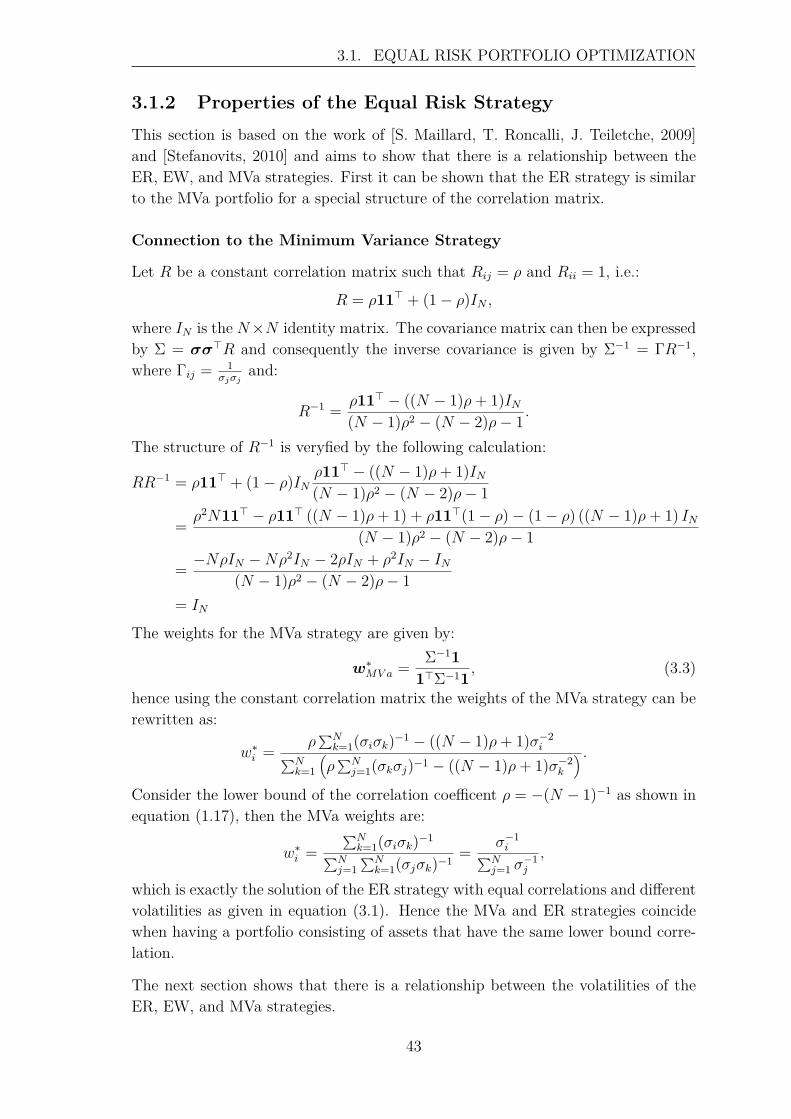
3.1. EQUAL RISK PORTFOLIO OPTIMIZATION
3.1.2 Properties of the Equal Risk StrategyThis section is based on the work of [S. Maillard, T. Roncalli, J. Teiletche, 2009]and [Stefanovits, 2010] and aims to show that there is a relationship between theER, EW, and MVa strategies. First it can be shown that the ER strategy is similarto the MVa portfolio for a special structure of the correlation matrix.
Connection to the Minimum Variance Strategy
Let R be a constant correlation matrix such that Rij = ρ and Rii = 1, i.e.:
R = ρ11> + (1− ρ)IN ,
where IN is the N×N identity matrix. The covariance matrix can then be expressedby Σ = σσ>R and consequently the inverse covariance is given by Σ−1 = ΓR−1,where Γij = 1
σjσjand:
R−1 = ρ11> − ((N − 1)ρ+ 1)IN(N − 1)ρ2 − (N − 2)ρ− 1 .
The structure of R−1 is veryfied by the following calculation:
RR−1 = ρ11> + (1− ρ)INρ11> − ((N − 1)ρ+ 1)IN(N − 1)ρ2 − (N − 2)ρ− 1
= ρ2N11> − ρ11> ((N − 1)ρ+ 1) + ρ11>(1− ρ)− (1− ρ) ((N − 1)ρ+ 1) IN(N − 1)ρ2 − (N − 2)ρ− 1
= −NρIN −Nρ2IN − 2ρIN + ρ2IN − IN
(N − 1)ρ2 − (N − 2)ρ− 1= IN
The weights for the MVa strategy are given by:
w∗MV a = Σ−111>Σ−11
, (3.3)
hence using the constant correlation matrix the weights of the MVa strategy can berewritten as:
w∗i = ρ∑Nk=1(σiσk)−1 − ((N − 1)ρ+ 1)σ−2
i∑Nk=1
(ρ∑Nj=1(σkσj)−1 − ((N − 1)ρ+ 1)σ−2
k
) .Consider the lower bound of the correlation coefficent ρ = −(N − 1)−1 as shown inequation (1.17), then the MVa weights are:
w∗i =∑Nk=1(σiσk)−1∑N
j=1∑Nk=1(σjσk)−1 = σ−1
i∑Nj=1 σ
−1j
,
which is exactly the solution of the ER strategy with equal correlations and differentvolatilities as given in equation (3.1). Hence the MVa and ER strategies coincidewhen having a portfolio consisting of assets that have the same lower bound corre-lation.
The next section shows that there is a relationship between the volatilities of theER, EW, and MVa strategies.
43
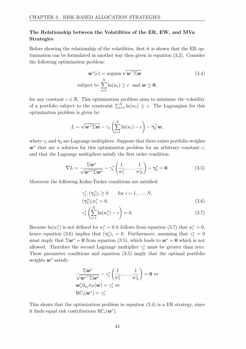
CHAPTER 3. RISK-BASED ALLOCATION STRATEGIES
The Relationship between the Volatilities of the ER, EW, and MVaStrategies
Before showing the relationship of the volatilities, first it is shown that the ER op-timization can be formulated in another way then given in equation (3.2). Considerthe following optimization problem:
w∗(c) = argmin√w>Σw (3.4)
subject toN∑i=1
ln(wi) ≥ c and w ≥ 0,
for any constant c ∈ R. This optimization problem aims to minimize the volatilityof a portfolio subject to the constraint ∑N
i=1 ln(wi) ≥ c. The Lagrangian for thisoptimization problem is given by:
L =√w>Σw − γ1
(N∑i=1
ln(wi)− c)− γ>2 w,
where γ1 and γ2 are Lagrange multipliers. Suppose that there exists portfolio weightsw∗ that are a solution for this optimization problem for an arbitrary constant c,and that the Lagrange multipliers satisfy the first order condition:
∇L = Σw∗√w∗>Σw∗
− γ∗1
(1w∗1, . . . ,
1w∗N
)− γ∗2 = 0. (3.5)
Moreover the following Kuhn-Tucker conditions are satisfied:
γ∗1 , (γ∗2)i ≥ 0 for i = 1, . . . , N,(γ∗2)iw∗i = 0, (3.6)
γ∗1
(N∑i=1
ln(w∗i )− c)
= 0. (3.7)
Because ln(w∗i ) is not defined for w∗i = 0 it follows from equation (3.7) that w∗i > 0,hence equation (3.6) implies that (γ∗2)i = 0. Furthermore, assuming that γ∗1 = 0must imply that Σw∗ = 0 from equation (3.5), which leads to w∗ = 0 which is notallowed. Therefore the second Lagrange multiplier γ∗1 must be greater than zero.These parameter conditions and equation (3.5) imply that the optimal portfolioweights w∗ satisfy:
Σw∗√w∗>Σw∗
− γ∗1
(1w∗1, . . . ,
1w∗N
)= 0⇔
w∗i ∂wiσP (w) = γ∗1 ⇔
RCi(w∗) = γ∗1 .
This shows that the optimization problem in equation (3.4) is a ER strategy, sinceit finds equal risk contributions RCi(w∗).
44
3.1. EQUAL RISK PORTFOLIO OPTIMIZATION
The portfolio weights also have to satisfy 1>w∗ = 1, therefore the portfolio weightsare normalized:
w∗i = w∗i (c)∑Ni=1w
∗i (c)
. (3.8)
Now in order to show the relationship of the volatilities of the MVa, ER, and EWstrategies suppose that c1 ≤ c2 then σP (w∗(c1)) ≤ σP (w∗(c2)), since ∑N
i=1 ln(wi)−c1 ≥ 0 is less restrictive than ∑N
i=1 ln(wi)− c2 ≥ 0.
In the case of c = −∞ the optimization problem in equation (3.4) yields the MVaportfolio since the inequality constraint disappears. On the other hand, when c =−N ln(N) then the optimization problem is the EW portfolio, which follows fromJensen’s inequality and the constraint 1>w = 1:
1N
N∑i=1
ln(wi) ≤ ln(
1N
N∑i=1
wi
)= − ln(N),
which implies that∑Ni=1 ln(wi) ≤ −N ln(N), hence σP (w∗(−∞)) ≤ σP (w∗(−N ln(N))).
For a general c ∈ [−∞,−N ln(N)] it therefore must hold that:
σP (w∗(−∞)) ≤σP (w∗(c)) ≤ σP (w∗(−N ln(N)))σMVa(w) ≤σER(w) ≤ σEW(w). (3.9)
This means that the MVa strategy is the less volatile strategy, the EW strategyis more volatile, and the ER strategy lies between both. Note that the portfoliovariances for the MVa and the EW strategy are given by:
σ2MVa(w) = 1
1>Σ1and σ2
EW(w) = N−1σ2•(1− ρ) + ρσ•, (3.10)
where the expression for σ2MVa(w) follows from equations (1.5) and (3.3), and σ2
EW(w)is derived in Example 1. There is no closed-form solution for the portfolio varianceσ2ER(w), since it depends on the variance and correlation structure of the assets in
a portfolio, as discussed in Section 3.1.1. But now it is known that it is boundedbelow and above.
The following example considers again the case of two assets and shows the rela-tionship of the portfolio weights for the three strategies.
45
CHAPTER 3. RISK-BASED ALLOCATION STRATEGIES
Example 3 (Two asset case - continued)Example 2 showed that the weights for the ER strategy are given by:
w∗ER =(
σ1
σ1 + σ2,
σ2
σ1 + σ2
).
It is known that the portfolio weights for the MVa strategy minimize the portfoliovariance, which is given by:
σ2P (w) = (w, 1− w)
[σ2
1 ρσ1σ2
ρσ1σ2 σ22
](w
1− w
)= σ1w
2 + 2ρσ1σ2w(1− w) + σ22(1− w)2.
So in order to find the the weights that minimize the portfolio variance σ2P (w) the
first order derivative with respect to w is determined:
d
dwσ2P (w) = 2w(σ2
1 − 2ρσ1σ2 + σ22) + 2ρσ1σ2 − 2σ2
2 ⇔
w = σ22 − ρσ1σ2
σ21 − 2ρσ1σ2 + σ2
2.
In order to verify that these weights find the minimum variance, the second orderderivative is determined:
d2
dw2σ2P (w) = 2(σ2
1 − 2ρσ1σ2 + σ22).
Since ρ ≤ 1 the second order derivative can be rewritten as:
2(σ21 − 2ρσ1σ2 + σ2
2) ≥ 2(σ21 − 2σ1σ2 + σ2
2) = 2(σ1 − σ2)2 ≥ 0,
which verifies that w minimizes σ2P (w), hence the portfolio weights for the MVa
strategy are given by:
w∗MV a = 1σ1 − 2ρσ1σ2 + σ2
2
(σ2
2 − ρσ1σ2, σ21 − ρσ1σ2
).
For the EW strategy the weights simply are:
w∗EW =(1
2 ,12
).
It can be seen that when σ1 = σ2 the weights of the three strategies are the same:
w∗MV a = w∗ER = w∗EW .
This statement is also shown in Figure 3.1. Furthermore, when ρ = −1 thenw∗MV a = w∗ER, which corresponds exactly to the case of the lowest possible cor-relation coefficent as shown in the start of this section. 4
46
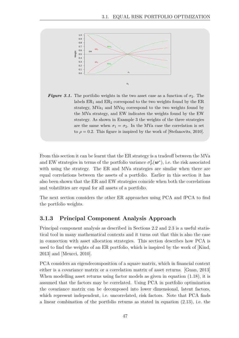
3.1. EQUAL RISK PORTFOLIO OPTIMIZATION
σ2
Wei
ght
0.0
0.1
0.2
0.3
0.4
0.5
0.6
0.7
0.8
0.9
1.0
σ1
ER2
ER1
MVa2
MVa1
EW
Figure 3.1. The portfolio weights in the two asset case as a function of σ2. Thelabels ER1 and ER2 correspond to the two weights found by the ERstrategy, MVa1 and MVa2 correspond to the two weights found bythe MVa strategy, and EW indicates the weights found by the EWstrategy. As shown in Example 3 the weights of the three strategiesare the same when σ1 = σ2. In the MVa case the correlation is setto ρ = 0.2. This figure is inspired by the work of [Stefanovits, 2010].
From this section it can be learnt that the ER strategy is a tradeoff between the MVaand EW strategies in terms of the portfolio variance σ2
P (w∗), i.e. the risk associatedwith using the strategy. The ER and MVa strategies are similar when there areequal correlations between the assets of a portfolio. Earlier in this section it hasalso been shown that the ER and EW strategies coincide when both the correlationsand volatilities are equal for all assets of a portfolio.
The next section considers the other ER approaches using PCA and fPCA to findthe portfolio weights.
3.1.3 Principal Component Analysis ApproachPrincipal component analysis as described in Sections 2.2 and 2.3 is a useful statis-tical tool in many mathematical contexts and it turns out that this is also the casein connection with asset allocation strategies. This section describes how PCA isused to find the weights of an ER portfolio, which is inspired by the work of [Kind,2013] and [Meucci, 2010].
PCA considers an eigendecomposition of a square matrix, which in financial contexteither is a covariance matrix or a correlation matrix of asset returns. [Guan, 2013]When modelling asset returns using factor models as given in equation (1.18), it isassumed that the factors may be correlated. Using PCA in portfolio optimizationthe covariance matrix can be decomposed into lower dimensional, latent factors,which represent independent, i.e. uncorrelated, risk factors. Note that PCA findsa linear combination of the portfolio returns as stated in equation (2.13), i.e. the
47
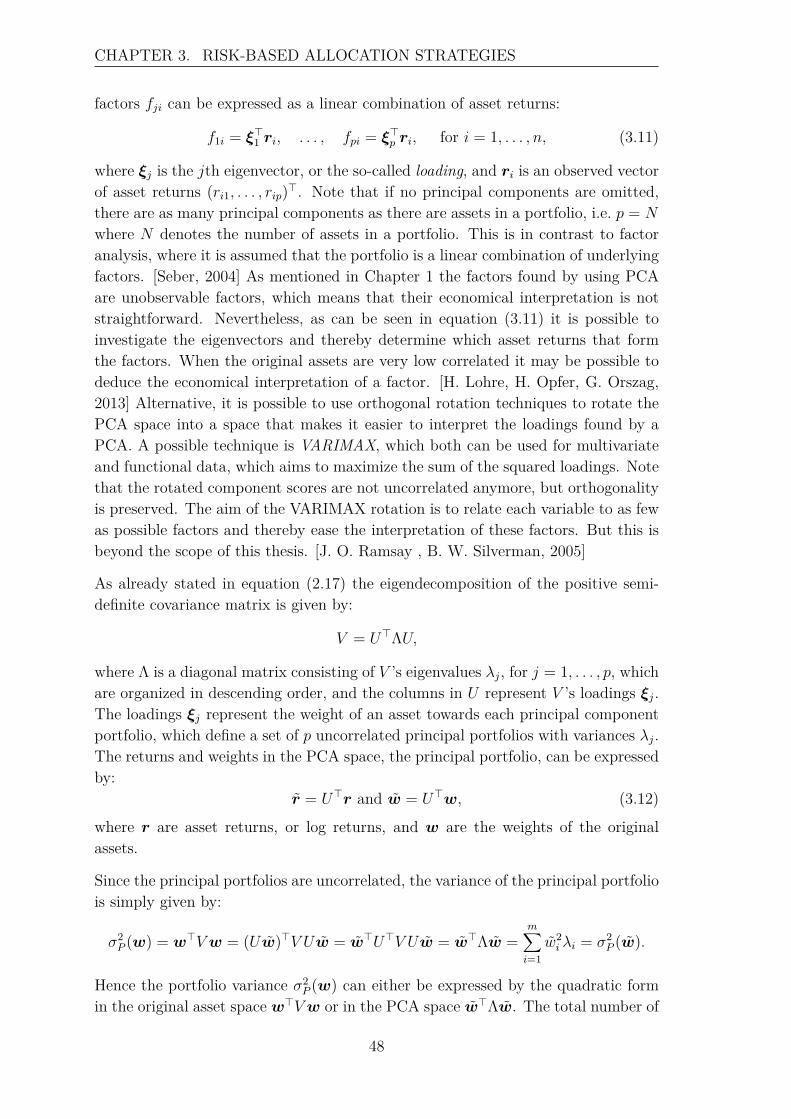
CHAPTER 3. RISK-BASED ALLOCATION STRATEGIES
factors fji can be expressed as a linear combination of asset returns:
f1i = ξ>1 ri, . . . , fpi = ξ>p ri, for i = 1, . . . , n, (3.11)
where ξj is the jth eigenvector, or the so-called loading, and ri is an observed vectorof asset returns (ri1, . . . , rip)>. Note that if no principal components are omitted,there are as many principal components as there are assets in a portfolio, i.e. p = N
where N denotes the number of assets in a portfolio. This is in contrast to factoranalysis, where it is assumed that the portfolio is a linear combination of underlyingfactors. [Seber, 2004] As mentioned in Chapter 1 the factors found by using PCAare unobservable factors, which means that their economical interpretation is notstraightforward. Nevertheless, as can be seen in equation (3.11) it is possible toinvestigate the eigenvectors and thereby determine which asset returns that formthe factors. When the original assets are very low correlated it may be possible todeduce the economical interpretation of a factor. [H. Lohre, H. Opfer, G. Orszag,2013] Alternative, it is possible to use orthogonal rotation techniques to rotate thePCA space into a space that makes it easier to interpret the loadings found by aPCA. A possible technique is VARIMAX, which both can be used for multivariateand functional data, which aims to maximize the sum of the squared loadings. Notethat the rotated component scores are not uncorrelated anymore, but orthogonalityis preserved. The aim of the VARIMAX rotation is to relate each variable to as fewas possible factors and thereby ease the interpretation of these factors. But this isbeyond the scope of this thesis. [J. O. Ramsay , B. W. Silverman, 2005]
As already stated in equation (2.17) the eigendecomposition of the positive semi-definite covariance matrix is given by:
V = U>ΛU,
where Λ is a diagonal matrix consisting of V ’s eigenvalues λj, for j = 1, . . . , p, whichare organized in descending order, and the columns in U represent V ’s loadings ξj.The loadings ξj represent the weight of an asset towards each principal componentportfolio, which define a set of p uncorrelated principal portfolios with variances λj.The returns and weights in the PCA space, the principal portfolio, can be expressedby:
r = U>r and w = U>w, (3.12)
where r are asset returns, or log returns, and w are the weights of the originalassets.
Since the principal portfolios are uncorrelated, the variance of the principal portfoliois simply given by:
σ2P (w) = w>Vw = (Uw)>V Uw = w>U>V Uw = w>Λw =
m∑i=1
w2i λi = σ2
P (w).
Hence the portfolio variance σ2P (w) can either be expressed by the quadratic form
in the original asset space w>Vw or in the PCA space w>Λw. The total number of
48
3.1. EQUAL RISK PORTFOLIO OPTIMIZATION
principal portfolios equals the number of considered principal components m. Themarginal risk contributions in the PCA space are given by:
∂wiσP (w) = 1
2√∑m
i=1 w2i λi
2wiλi = wiλiσP (w) .
Moreover, since in the PCA space the covariance matrix has covariances that equalzero, the risk contributions RCi in the principal space must be equal to:
RCi = w2i λi√∑m
i=1 w2i λi
Hence a similar optimization problem to Section 3.1 can be formulated:
w∗ = argmin f(w) (3.13)subject to 1>w = 1 and 0 ≤ w ≤ 1,
wheref(w) =
m∑i=1
m∑j=1
(RCi − RCj
)2.
The zero covariances in the PCA space also imply that the weights can be expressedby a closed-form solution similar to equation (3.1). Thus the optimal weights in thePCA space are given by:
w∗i = (√λi)−1∑m
i=1(√λi)−1 . (3.14)
Another way of formulating the ER approach is inspired by the work of Jyske Bank,where the principal portfolios found are used to construct a diversified portfolio insuch a way that the weights are chosen to yield as equal as possible volatilities in eachcomponent. So the aim of the optimization is to have equal risk in all directions ofrisk. The risk in a direction is defined as the amount of risk of the overall risk that isfound in the given direction, where risk is proportional to the variance, i.e. are givenby the eigenvalues in each direction. In order to hold a well-diversified portfolio itsoverall risk should be evenly spread across the principal portfolios. Jyske Bank hasestablished the following objective function:
minw
m∑i=1
CPVi subject to 1>w = 1 and − 1 ≤ w ≤ 1, (3.15)
where CPVi is the ith cumulative proportion of variance from the PCA as definedin equation (2.35). The objective function is the sum of every principal component’scumulative proportion of variance. This means by minimizing equation (3.15), theproportion of variances are made as equal as possible, which corresponds to haveequal risk in each component. An example of the cumulative proportion of eachcomponent can be seen in Figure 3.2.
49
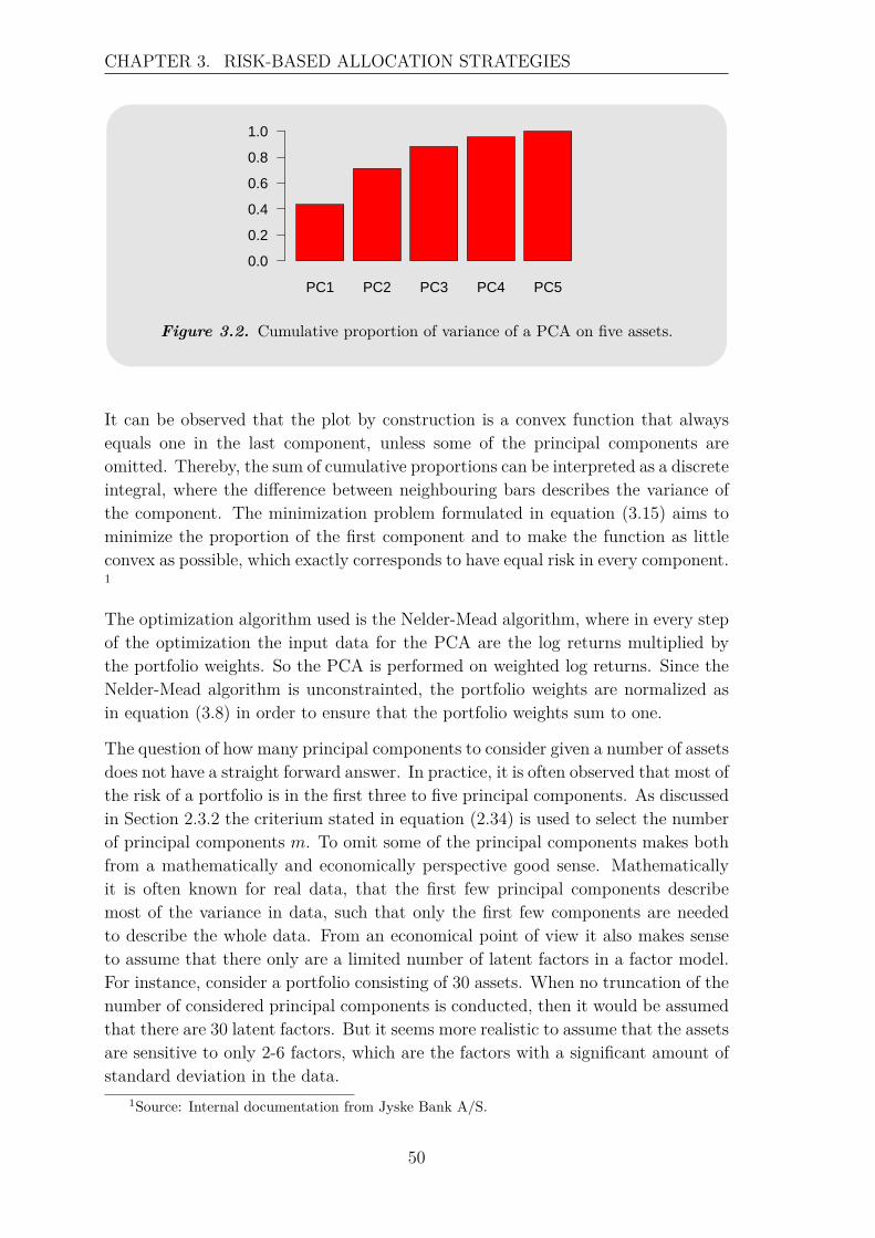
CHAPTER 3. RISK-BASED ALLOCATION STRATEGIES
PC1 PC2 PC3 PC4 PC5
Cumulative Proportion
0.0
0.2
0.4
0.6
0.8
1.0
Figure 3.2. Cumulative proportion of variance of a PCA on five assets.
It can be observed that the plot by construction is a convex function that alwaysequals one in the last component, unless some of the principal components areomitted. Thereby, the sum of cumulative proportions can be interpreted as a discreteintegral, where the difference between neighbouring bars describes the variance ofthe component. The minimization problem formulated in equation (3.15) aims tominimize the proportion of the first component and to make the function as littleconvex as possible, which exactly corresponds to have equal risk in every component.1
The optimization algorithm used is the Nelder-Mead algorithm, where in every stepof the optimization the input data for the PCA are the log returns multiplied bythe portfolio weights. So the PCA is performed on weighted log returns. Since theNelder-Mead algorithm is unconstrainted, the portfolio weights are normalized asin equation (3.8) in order to ensure that the portfolio weights sum to one.
The question of how many principal components to consider given a number of assetsdoes not have a straight forward answer. In practice, it is often observed that most ofthe risk of a portfolio is in the first three to five principal components. As discussedin Section 2.3.2 the criterium stated in equation (2.34) is used to select the numberof principal components m. To omit some of the principal components makes bothfrom a mathematically and economically perspective good sense. Mathematicallyit is often known for real data, that the first few principal components describemost of the variance in data, such that only the first few components are neededto describe the whole data. From an economical point of view it also makes senseto assume that there only are a limited number of latent factors in a factor model.For instance, consider a portfolio consisting of 30 assets. When no truncation of thenumber of considered principal components is conducted, then it would be assumedthat there are 30 latent factors. But it seems more realistic to assume that the assetsare sensitive to only 2-6 factors, which are the factors with a significant amount ofstandard deviation in the data.
1Source: Internal documentation from Jyske Bank A/S.
50
3.1. EQUAL RISK PORTFOLIO OPTIMIZATION
The next section expands the ER approach to make use of functional principalcomponent analysis. The reason for considering this approach is, that it is assumedto capture the variability in assets returns better, since it makes use of the underlyingfunctional form the returns, and thereby may find more accurate portfolio weights.
Functional Principal Component Analysis Approach
Functional principal component analysis, fPCA, considers data to have an under-lying functional form that can be modelled by univariate functions as explained inSection 2.3. This makes it possible to observe the behaviour of the eigenfunctionsover time in contrast to PCA that just gives a static, non-temporal estimate of theeigenvectors. That is, it is possible to see the features characterizing asset returnsover a period of time.
In order to obtain an ER portfolio using fPCA, a similar optimization problem asgiven in equation (3.15) is solved. Hence the ER approach of finding equal volatilitiesin the components is considered. The reason to only consider this approach isbecause it is not known how the functional variant will perform in a backtest, soonly one of the ER approaches is investigated for possible improvements. Thedifference to the PCA is that fPCA should be better in taking into account thevariation of the asset returns over time.
To make use of fPCA first data has to be transformed to functional data and to besmoothed as explained in Section 2.1.2. The basis functions used for the roughnesspenalty matrix R are equally spaced B-splines. So one has to determine the numberof B-splines K and the smoothing parameter λ.
The number of basis functions is chosen by a three-fold cross validation. Thismeans that data is divided into three equally sized sets, where two of the sets areused to train different values of K and the last set is used to validate the foundK values. Simultaneously, there is performed a five-fold cross validation for λ onthe trainings sets of the basis functions, again by dividing the training set into fiveequally spaced sets. The reason that the cross validation for λ is embedded in thecross validation for K is because the smoothing parameter λ depends on the numberof basis functions K. The setup is illustrated in Figure 3.3. Hence for every trainedK value there is a corresponding λ value. Then the two trained K values with theircorresponding λ are tested on the validation set. The criterium used to find the bestK and λ is the GCV(λ) as given in equation (2.11). The GCV statistic is used withinthe performed three- and five-fold cross validation, since it is an approximation toleave-one-out cross validation as explained in Section 2.1.2. Furthermore a rollingwindow is used, where the first part of data is used as trainings set and the lastpart of data for validation, which should give better parameter estimates whencalculating the portfolio weights today. This also means that this setup might notbe completely proper when used in a backtest.
51
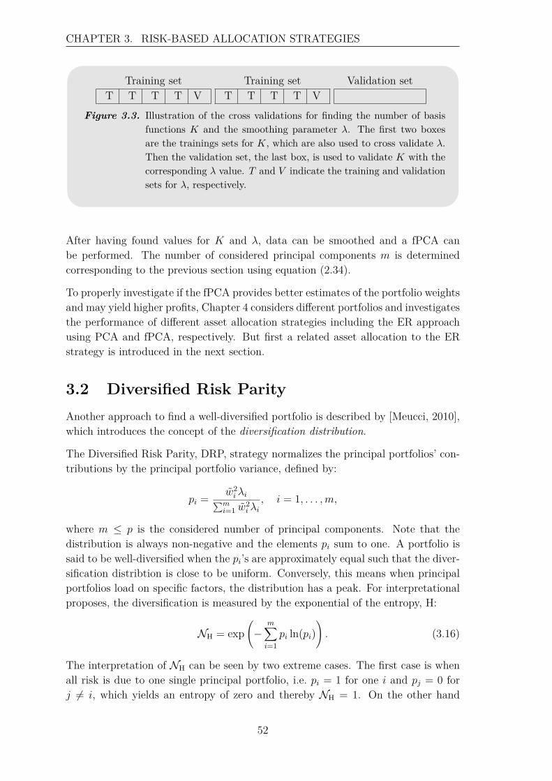
CHAPTER 3. RISK-BASED ALLOCATION STRATEGIES
Training setT T T T V
Training setT T T T V
Validation set
Figure 3.3. Illustration of the cross validations for finding the number of basisfunctions K and the smoothing parameter λ. The first two boxesare the trainings sets for K, which are also used to cross validate λ.Then the validation set, the last box, is used to validate K with thecorresponding λ value. T and V indicate the training and validationsets for λ, respectively.
After having found values for K and λ, data can be smoothed and a fPCA canbe performed. The number of considered principal components m is determinedcorresponding to the previous section using equation (2.34).
To properly investigate if the fPCA provides better estimates of the portfolio weightsand may yield higher profits, Chapter 4 considers different portfolios and investigatesthe performance of different asset allocation strategies including the ER approachusing PCA and fPCA, respectively. But first a related asset allocation to the ERstrategy is introduced in the next section.
3.2 Diversified Risk ParityAnother approach to find a well-diversified portfolio is described by [Meucci, 2010],which introduces the concept of the diversification distribution.
The Diversified Risk Parity, DRP, strategy normalizes the principal portfolios’ con-tributions by the principal portfolio variance, defined by:
pi = w2i λi∑m
i=1 w2i λi
, i = 1, . . . ,m,
where m ≤ p is the considered number of principal components. Note that thedistribution is always non-negative and the elements pi sum to one. A portfolio issaid to be well-diversified when the pi’s are approximately equal such that the diver-sification distribtion is close to be uniform. Conversely, this means when principalportfolios load on specific factors, the distribution has a peak. For interpretationalproposes, the diversification is measured by the exponential of the entropy, H:
NH = exp(−
m∑i=1
pi ln(pi)). (3.16)
The interpretation of NH can be seen by two extreme cases. The first case is whenall risk is due to one single principal portfolio, i.e. pi = 1 for one i and pj = 0 forj 6= i, which yields an entropy of zero and thereby NH = 1. On the other hand
52
3.2. DIVERSIFIED RISK PARITY
if one holds a homogenous portfolio where pi = m−1 for all i, the entropy equalsln(m), such that the maximium value of NH = m.
The optimization problem to be solved is given by:
arg maxwNH (3.17)
subject to 1>w = 1 and − 1 ≤ w ≤ 1.
Hence it is a nonlinear problem with constraints which could be solved using a SQPoptimization algorithm as explained in Section 3.1.1.
The difference between the ER and DRP approaches is that they are based on twodifferent measures of risk. The ER approach aims to diversify a portfolio such thatthe risk contributions are equal. On the other hand, the DRP approach defines awell-diversified portfolio such that the elements pi of the diversification distributionare uniform distributed. [A. Meucci, A. Santangelo, R. Deguest, 2014] But withoutany further constraints the solutions to the optimization problems given in equation(3.13) and equation (3.17) coincide. This is due to the fact that the risk contributionsin the PCA space RCi are almost equal to the diversifications distribution elementspi, so in this case the ER and DRP approaches optimize a similar problem just withdifferent objective functions. This will also be shown in the simulation study inSection 3.4.2. Table 3.1 summarizes some of the important notations in the assetand principal space, respectively.
Table 3.1. Notions in the asset space and in the PCA space. This table is inspired by[Kind, 2013].
Asset Space Principal Space
Weights wi wi
Portfolio Variance σ2P (w) = ∑N
i=1w2i σ
2i +∑6=
i,j wiwjσij σ2P (w) = ∑m
i=1 w2i λi
Marginal Risk ∂wiσP (w) = wiσ
2i +∑
i 6=jwjσij
σP (w) ∂wiσP (w) = wiλi
σP (w)Contribution
Risk RCi = w2i σ
2i +∑
i6=jwiwjσij
σP (w) RCi = w2i λi
σP (w)Contribution
The next section shows that the traditional allocation strategies EW and MVa asintroduced in Chapter 1 also can be considered in the PCA space.
53
CHAPTER 3. RISK-BASED ALLOCATION STRATEGIES
3.3 The Equally-Weighted and MinimumVariance Strategies using PrincipalPortfolios
The strategies EW and MVa can also be performed in the PCA space. This sectiongives a short introduction to these approaches and is based on the work of [Kind,2013], but they will not be considered in the backtest performed in Chapter 4. Theportfolio weights of the EW strategy used on the principal portfolio are given by:
w∗i = m−1 for i = 1, . . . ,m,
where m is the number of principal components. In the PCA space the EW strategyprobably is a very bad diversification strategy, since the variance of each principalportfolio is given by the eigenvalues λi. It is known that eigenvalues are chosen to bevariance maximizing and of decreasing order, hence using the EW strategy will givea very unbalanced risk distribution of the principal portfolio. Based on equation(3.3) the portfolio weights of the MVa strategy in the PCA space can be expressedby:
w∗i = λ−1i∑m
i=1 λ−1i
.
From equation (3.10) it follows that the portfolio variances in the PCA space forthe MVa and the EW strategy are given by:
σ2MV(w) = 1∑m
i=1 λ−1i
and σ2EW(w) = m−1λ•,
where λ• is the average of the principal portfolio variances. Similar to the propertyof the portfolio volatilities in equation (3.9), it can be shown that the same propertyapplies for the portfolio volatilities in the PCA space:
σMV(w) ≤ σER(w) ≤ σEW(w),
where the ER strategy using risk contributions in the PCA space, ER- PCA RC,as given in equation (3.13) is considered. For a proof of this statement see [Kind,2013]. Since it is known that the assets in the PCA space are uncorrelated and mayhave different volatilites, there is an explicit expression for the portfolio variance inthe ER approach. Hence using the expression for the portfolio variance in the PCAspace as stated in Table 3.1 with the portfolio weights from equation (3.14), theportfolio variance for the ER- PCA RC strategy is given by:
σ2ER(w) = m(∑m
i=1(√λi)−1
)2 .
This section shows that the relation between the portfolio volatilities of the threestrategies: MVa, ER, and EW is valid both in the original asset space as well as inthe PCA space.
54
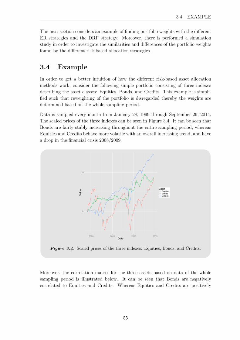
3.4. EXAMPLE
The next section considers an example of finding portfolio weights with the differentER strategies and the DRP strategy. Moreover, there is performed a simulationstudy in order to investigate the similarities and differences of the portfolio weightsfound by the different risk-based allocation strategies.
3.4 ExampleIn order to get a better intuition of how the different risk-based asset allocationmethods work, consider the following simple portfolio consisting of three indexesdescribing the asset classes: Equities, Bonds, and Credits. This example is simpli-fied such that reweighting of the portfolio is disregarded thereby the weights aredetermined based on the whole sampling period.
Data is sampled every month from January 28, 1999 through September 29, 2014.The scaled prices of the three indexes can be seen in Figure 3.4. It can be seen thatBonds are fairly stably increasing throughout the entire sampling period, whereasEquities and Credits behave more volatile with an overall increasing trend, and havea drop in the financial crisis 2008/2009.
1
2
2000 2005 2010 2015Date
Val
ue
AssetEquitiesBondsCredits
Index − Portfolio Components
Figure 3.4. Scaled prices of the three indexes: Equities, Bonds, and Credits.
Moreover, the correlation matrix for the three assets based on data of the wholesampling period is illustrated below. It can be seen that Bonds are negativelycorrelated to Equities and Credits. Whereas Equities and Credits are positively
55
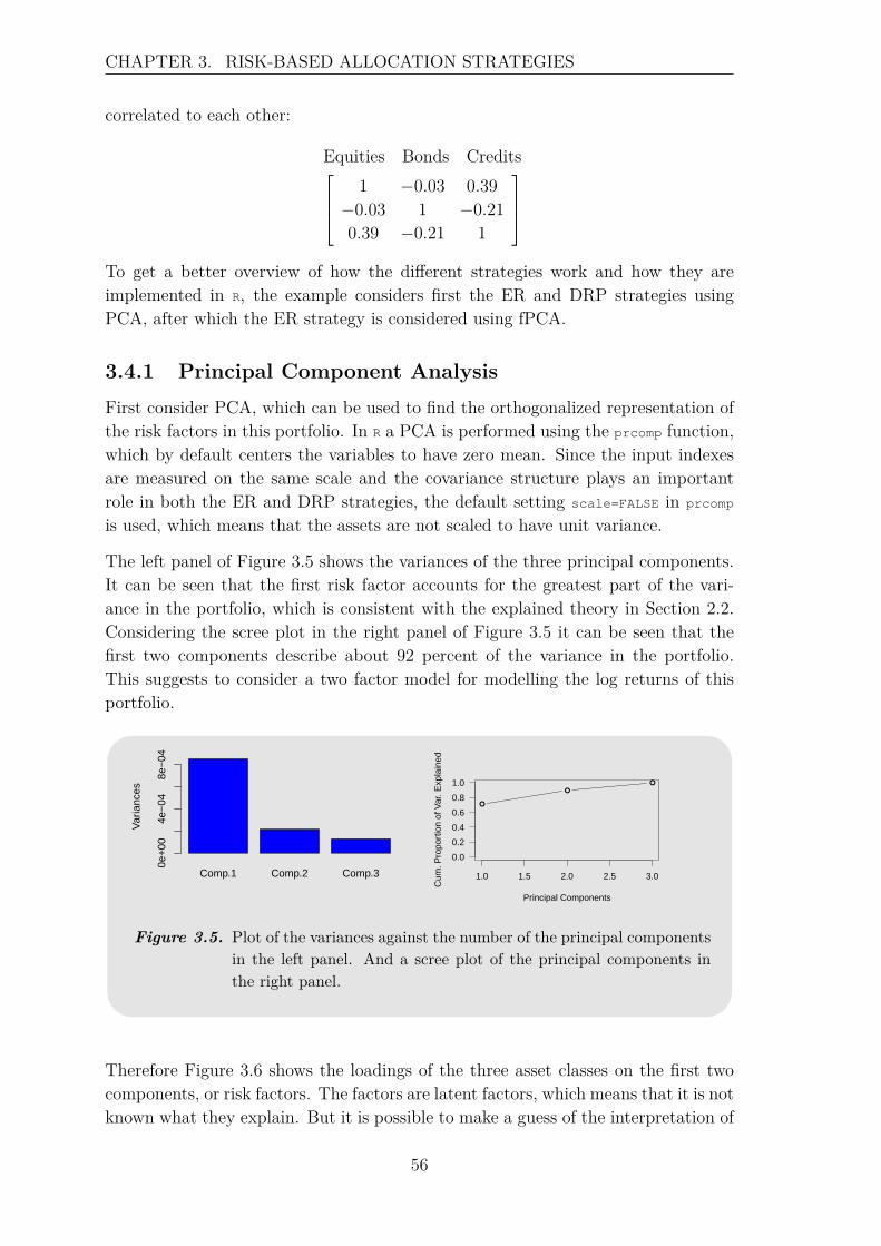
CHAPTER 3. RISK-BASED ALLOCATION STRATEGIES
correlated to each other:
Equities Bonds Credits1 −0.03 0.39
−0.03 1 −0.210.39 −0.21 1
To get a better overview of how the different strategies work and how they areimplemented in R, the example considers first the ER and DRP strategies usingPCA, after which the ER strategy is considered using fPCA.
3.4.1 Principal Component AnalysisFirst consider PCA, which can be used to find the orthogonalized representation ofthe risk factors in this portfolio. In R a PCA is performed using the prcomp function,which by default centers the variables to have zero mean. Since the input indexesare measured on the same scale and the covariance structure plays an importantrole in both the ER and DRP strategies, the default setting scale=FALSE in prcomp
is used, which means that the assets are not scaled to have unit variance.
The left panel of Figure 3.5 shows the variances of the three principal components.It can be seen that the first risk factor accounts for the greatest part of the vari-ance in the portfolio, which is consistent with the explained theory in Section 2.2.Considering the scree plot in the right panel of Figure 3.5 it can be seen that thefirst two components describe about 92 percent of the variance in the portfolio.This suggests to consider a two factor model for modelling the log returns of thisportfolio.
Comp.1 Comp.2 Comp.3
PCA
Var
ianc
es
0e+
004e
−04
8e−
04
Principal Components
Cum
. Pro
port
ion
of V
ar. E
xpla
ined
1.0 1.5 2.0 2.5 3.0
0.0
0.2
0.4
0.6
0.8
1.0
Figure 3.5. Plot of the variances against the number of the principal componentsin the left panel. And a scree plot of the principal components inthe right panel.
Therefore Figure 3.6 shows the loadings of the three asset classes on the first twocomponents, or risk factors. The factors are latent factors, which means that it is notknown what they explain. But it is possible to make a guess of the interpretation of
56
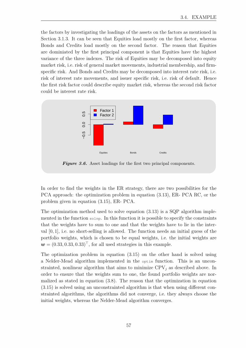
3.4. EXAMPLE
the factors by investigating the loadings of the assets on the factors as mentioned inSection 3.1.3. It can be seen that Equities load mostly on the first factor, whereasBonds and Credits load mostly on the second factor. The reason that Equitiesare dominiated by the first principal component is that Equities have the highestvariance of the three indexes. The risk of Equities may be decomposed into equitymarket risk, i.e. risk of general market movements, industrial membership, and firm-specific risk. And Bonds and Credits may be decomposed into interest rate risk, i.e.risk of interest rate movements, and issuer specific risk, i.e. risk of default. Hencethe first risk factor could describe equity market risk, whereas the second risk factorcould be interest rate risk.
Equities Bonds Credits
−0.
50.
00.
5 Factor 1Factor 2
Figure 3.6. Asset loadings for the first two principal components.
In order to find the weights in the ER strategy, there are two possibilities for thePCA approach: the optimization problem in equation (3.13), ER- PCA RC, or theproblem given in equation (3.15), ER- PCA.
The optimization method used to solve equation (3.13) is a SQP algorithm imple-mented in the function solnp. In this function it is possible to specify the constraintsthat the weights have to sum to one and that the weights have to lie in the inter-val [0, 1], i.e. no short-selling is allowed. The function needs an initial guess of theportfolio weights, which is chosen to be equal weights, i.e. the initial weights arew = (0.33, 0.33, 0.33)>, for all used strategies in this example.
The optimization problem in equation (3.15) on the other hand is solved usinga Nelder-Mead algorithm implemented in the optim function. This is an uncon-strainted, nonlinear algorithm that aims to minimize CPVj as described above. Inorder to ensure that the weights sum to one, the found portfolio weights are nor-malized as stated in equation (3.8). The reason that the optimization in equation(3.15) is solved using an unconstrainted algorithm is that when using different con-strainted algorithms, the algorithms did not converge, i.e. they always choose theinitial weights, whereas the Nelder-Mead algorithm converges.
57
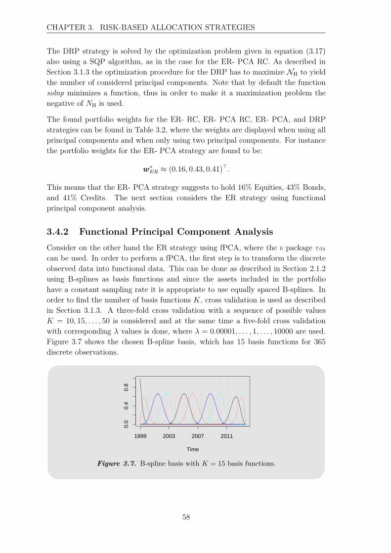
CHAPTER 3. RISK-BASED ALLOCATION STRATEGIES
The DRP strategy is solved by the optimization problem given in equation (3.17)also using a SQP algorithm, as in the case for the ER- PCA RC. As described inSection 3.1.3 the optimization procedure for the DRP has to maximize NH to yieldthe number of considered principal components. Note that by default the functionsolnp minimizes a function, thus in order to make it a maximization problem thenegative of NH is used.
The found portfolio weights for the ER- RC, ER- PCA RC, ER- PCA, and DRPstrategies can be found in Table 3.2, where the weights are displayed when using allprincipal components and when only using two principal components. For instancethe portfolio weights for the ER- PCA strategy are found to be:
w∗ER ≈ (0.16, 0.43, 0.41)>.
This means that the ER- PCA strategy suggests to hold 16% Equities, 43% Bonds,and 41% Credits. The next section considers the ER strategy using functionalprincipal component analysis.
3.4.2 Functional Principal Component AnalysisConsider on the other hand the ER strategy using fPCA, where the R package fda
can be used. In order to perform a fPCA, the first step is to transform the discreteobserved data into functional data. This can be done as described in Section 2.1.2using B-splines as basis functions and since the assets included in the portfoliohave a constant sampling rate it is appropriate to use equally spaced B-splines. Inorder to find the number of basis functions K, cross validation is used as describedin Section 3.1.3. A three-fold cross validation with a sequence of possible valuesK = 10, 15, . . . , 50 is considered and at the same time a five-fold cross validationwith corresponding λ values is done, where λ = 0.00001, . . . , 1, . . . , 10000 are used.Figure 3.7 shows the chosen B-spline basis, which has 15 basis functions for 365discrete observations.
Time
0.0
0.4
0.8
1999 2003 2007 2011
Figure 3.7. B-spline basis with K = 15 basis functions.
58
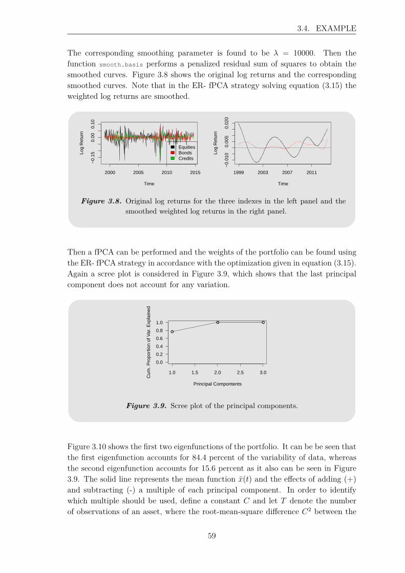
3.4. EXAMPLE
The corresponding smoothing parameter is found to be λ = 10000. Then thefunction smooth.basis performs a penalized residual sum of squares to obtain thesmoothed curves. Figure 3.8 shows the original log returns and the correspondingsmoothed curves. Note that in the ER- fPCA strategy solving equation (3.15) theweighted log returns are smoothed.
2000 2005 2010 2015
−0.
150.
000.
10
Time
Log
Ret
urn
EquitiesBondsCredits
Time
Log
Ret
urn
−0.
010
0.00
50.
020
1999 2003 2007 2011
Figure 3.8. Original log returns for the three indexes in the left panel and thesmoothed weighted log returns in the right panel.
Then a fPCA can be performed and the weights of the portfolio can be found usingthe ER- fPCA strategy in accordance with the optimization given in equation (3.15).Again a scree plot is considered in Figure 3.9, which shows that the last principalcomponent does not account for any variation.
Principal Compontents
Cum
. Pro
port
ion
of V
ar. E
xpla
ined
1.0 1.5 2.0 2.5 3.0
0.0
0.2
0.4
0.6
0.8
1.0
Figure 3.9. Scree plot of the principal components.
Figure 3.10 shows the first two eigenfunctions of the portfolio. It can be be seen thatthe first eigenfunction accounts for 84.4 percent of the variability of data, whereasthe second eigenfunction accounts for 15.6 percent as it also can be seen in Figure3.9. The solid line represents the mean function x(t) and the effects of adding (+)and subtracting (-) a multiple of each principal component. In order to identifywhich multiple should be used, define a constant C and let T denote the numberof observations of an asset, where the root-mean-square difference C2 between the
59
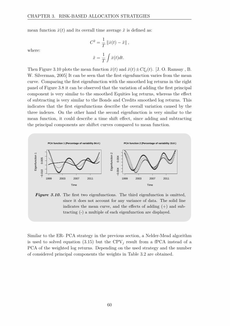
CHAPTER 3. RISK-BASED ALLOCATION STRATEGIES
mean function x(t) and its overall time average x is defined as:
C2 = 1T‖x(t)− x‖ ,
where:x = 1
T
∫x(t)dt.
Then Figure 3.10 plots the mean function x(t) and x(t)±Cξj(t). [J. O. Ramsay , B.W. Silverman, 2005] It can be seen that the first eigenfunction varies from the meancurve. Comparing the first eigenfunction with the smoothed log returns in the rightpanel of Figure 3.8 it can be observed that the variation of adding the first principalcomponent is very similar to the smoothed Equities log returns, whereas the effectof subtracting is very similar to the Bonds and Credits smoothed log returns. Thisindicates that the first eigenfunctions describe the overall variation caused by thethree indexes. On the other hand the second eigenfunction is very similar to themean function, it could describe a time shift effect, since adding and subtractingthe principal components are shiftet curves compared to mean function.
PCA function 1 (Percentage of variability 84.4 )
Time
Eig
enfu
nctio
n 1
++++++++++++++++++++++++++++++++++++++++++++++++++++++++++++++++++++++++++++++++++++
++++++++++++++++++++++++++++++++++
++++++++++
−−−−−−−−−−−−−−−−−−−−−−−−−−−−−−−−−−−−−−−−−−−−−−−−−−−−−−−−−−−−−−−−−−−−−−−−−−−
−−−−−−−−−−−
−−−−−−−−−−−−−−−−−−−−−−−−−−−−−−−−−−−−−−−−−−
−0.
010
0.00
5
1999 2003 2007 2011
PCA function 2 (Percentage of variability 15.6 )
Time
Eig
enfu
nctio
n 2 +++++++++++++++++++++++++++
++++++++++++++++++
+++++++++++++++++++++++++++++++++++++++++++++++++++++
++++++++++++++++++++++++++++++−−−−−−−−−−−−−−−−−−−−−−−−−−−−−−−−−
−−−−−−−−−−−−−−−−−
−−−−−−−−−−−−−−−−−−−−−−−−−−−−−−−−−−−−−−−−−−−
−−−−−−−−−−−−−−−−−−−−−−−−−−−−−−−−−−−
−0.
004
0.00
4
1999 2003 2007 2011
Figure 3.10. The first two eigenfunctions. The third eigenfunction is omitted,since it does not account for any variance of data. The solid lineindicates the mean curve, and the effects of adding (+) and sub-tracting (-) a multiple of each eigenfunction are displayed.
Similar to the ER- PCA strategy in the previous section, a Nelder-Mead algorithmis used to solved equation (3.15) but the CPVj result from a fPCA instead of aPCA of the weighted log returns. Depending on the used strategy and the numberof considered principal components the weights in Table 3.2 are obtained.
60
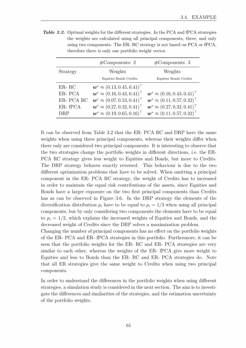
3.4. EXAMPLE
Table 3.2. Optimal weights for the different strategies. In the PCA and fPCA strategiesthe weights are calculated using all principal components, three, and onlyusing two components. The ER- RC strategy is not based on PCA or fPCA,therefore there is only one portfolio weight vector.
#Components: 2 #Components: 3
Strategy Weights WeightsEquities Bonds Credits Equities Bonds Credits
ER- RC w∗ ≈ (0.13, 0.45, 0.41)>ER- PCA w∗ ≈ (0.16, 0.43, 0.41)> w∗ ≈ (0.16, 0.43, 0.41)>ER- PCA RC w∗ ≈ (0.07, 0.53, 0.41)> w∗ ≈ (0.11, 0.57, 0.32)>ER- fPCA w∗ ≈ (0.27, 0.32, 0.41)> w∗ ≈ (0.27, 0.32, 0.41)>DRP w∗ ≈ (0.19, 0.65, 0.16)> w∗ ≈ (0.11, 0.57, 0.32)>
It can be observed from Table 3.2 that the ER- PCA RC and DRP have the sameweights when using three principal components, whereas their weights differ whenthere only are considered two principal components. It is interesting to observe thatthe two strategies change the portfolio weights in different directions, i.e. the ER-PCA RC strategy gives less weight to Equities and Bonds, but more to Credits.The DRP strategy behaves exactly reversed. This behaviour is due to the twodifferent optimization problems that have to be solved. When omitting a principalcomponent in the ER- PCA RC strategy, the weight of Credits has to increasedin order to maintain the equal risk contributions of the assets, since Equities andBonds have a larger exposure on the two first principal components than Creditshas as can be observed in Figure 3.6. In the DRP strategy the elements of thediversification distribution pi have to be equal to pi = 1/3 when using all principalcomponents, but by only considering two components the elements have to be equalto pi = 1/2, which explains the increased weights of Equities and Bonds, and thedecreased weight of Credits since the DRP solves a maximization problem.Changing the number of principal components has no effect on the portfolio weightsof the ER- PCA and ER- fPCA strategies in this portfolio. Furthermore, it can beseen that the portfolio weights for the ER- RC and ER- PCA strategies are verysimilar to each other, whereas the weights of the ER- fPCA give more weight toEquities and less to Bonds than the ER- RC and ER- PCA strategies do. Notethat all ER strategies give the same weight to Credits when using two principalcomponents.
In order to understand the differences in the portfolio weights when using differentstrategies, a simulation study is considered in the next section. The aim is to investi-gate the differences and similarities of the strategies, and the estimation uncertaintyof the portfolio weights.
61
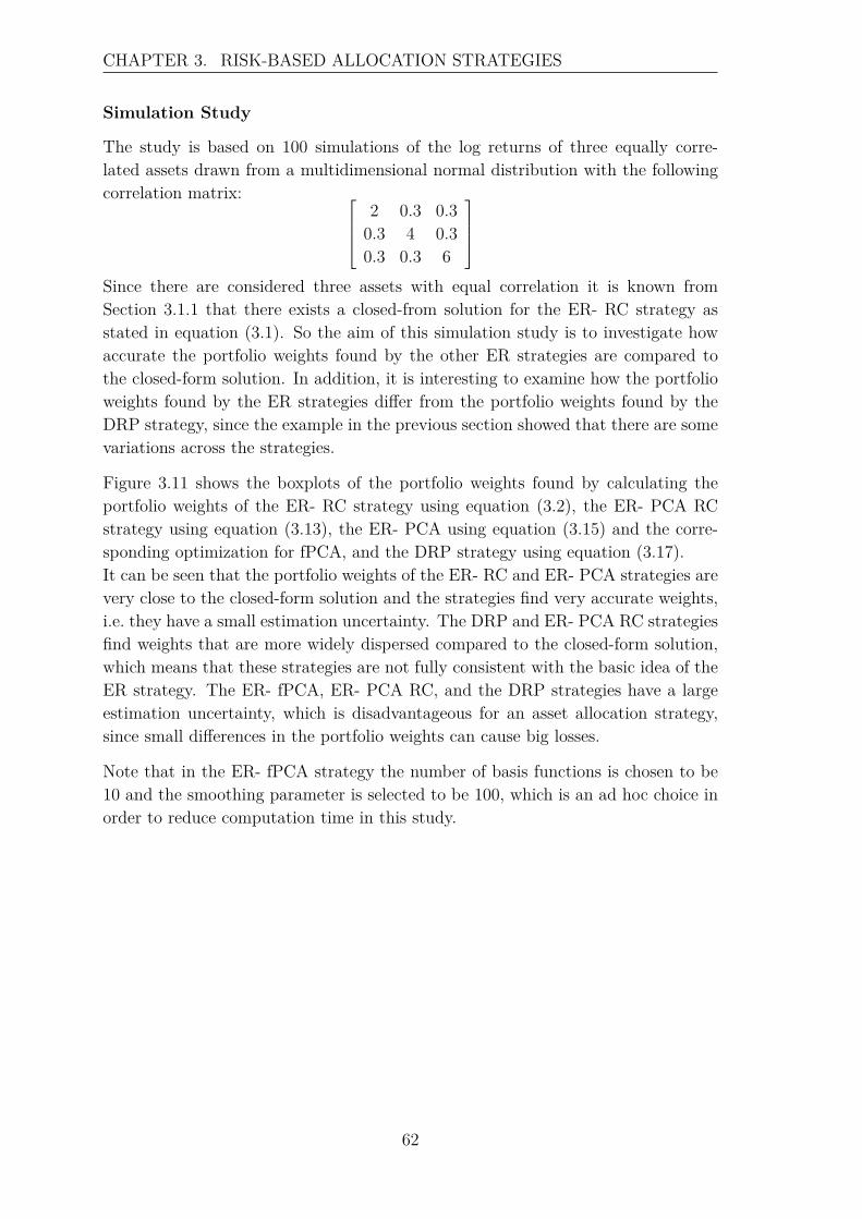
CHAPTER 3. RISK-BASED ALLOCATION STRATEGIES
Simulation Study
The study is based on 100 simulations of the log returns of three equally corre-lated assets drawn from a multidimensional normal distribution with the followingcorrelation matrix:
2 0.3 0.30.3 4 0.30.3 0.3 6
Since there are considered three assets with equal correlation it is known fromSection 3.1.1 that there exists a closed-from solution for the ER- RC strategy asstated in equation (3.1). So the aim of this simulation study is to investigate howaccurate the portfolio weights found by the other ER strategies are compared tothe closed-form solution. In addition, it is interesting to examine how the portfolioweights found by the ER strategies differ from the portfolio weights found by theDRP strategy, since the example in the previous section showed that there are somevariations across the strategies.
Figure 3.11 shows the boxplots of the portfolio weights found by calculating theportfolio weights of the ER- RC strategy using equation (3.2), the ER- PCA RCstrategy using equation (3.13), the ER- PCA using equation (3.15) and the corre-sponding optimization for fPCA, and the DRP strategy using equation (3.17).It can be seen that the portfolio weights of the ER- RC and ER- PCA strategies arevery close to the closed-form solution and the strategies find very accurate weights,i.e. they have a small estimation uncertainty. The DRP and ER- PCA RC strategiesfind weights that are more widely dispersed compared to the closed-form solution,which means that these strategies are not fully consistent with the basic idea of theER strategy. The ER- fPCA, ER- PCA RC, and the DRP strategies have a largeestimation uncertainty, which is disadvantageous for an asset allocation strategy,since small differences in the portfolio weights can cause big losses.
Note that in the ER- fPCA strategy the number of basis functions is chosen to be10 and the smoothing parameter is selected to be 100, which is an ad hoc choice inorder to reduce computation time in this study.
62
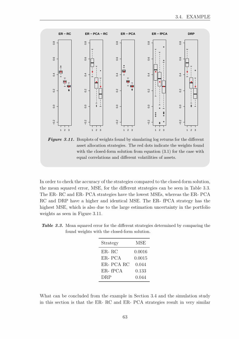
3.4. EXAMPLE
1 2 3
−0.
20.
00.
20.
40.
60.
8
ER − RC
1 2 3
−0.
20.
00.
20.
40.
60.
8
ER − PCA − RC
1 2 3
−0.
20.
00.
20.
40.
60.
8
ER − PCA
1 2 3
−0.
20.
00.
20.
40.
60.
8
ER − fPCA
1 2 3
−0.
20.
00.
20.
40.
60.
8
DRP
Figure 3.11. Boxplots of weights found by simulating log returns for the differentasset allocation strategies. The red dots indicate the weights foundwith the closed-form solution from equation (3.1) for the case withequal correlations and different volatilities of assets.
In order to check the accuracy of the strategies compared to the closed-form solution,the mean squared error, MSE, for the different strategies can be seen in Table 3.3.The ER- RC and ER- PCA strategies have the lowest MSEs, whereas the ER- PCARC and DRP have a higher and identical MSE. The ER- fPCA strategy has thehighest MSE, which is also due to the large estimation uncertainty in the portfolioweights as seen in Figure 3.11.
Table 3.3. Mean squared error for the different strategies determined by comparing thefound weights with the closed-form solution.
Strategy MSE
ER- RC 0.0016ER- PCA 0.0015ER- PCA RC 0.044ER- fPCA 0.133DRP 0.044
What can be concluded from the example in Section 3.4 and the simulation studyin this section is that the ER- RC and ER- PCA strategies result in very similar
63

CHAPTER 3. RISK-BASED ALLOCATION STRATEGIES
portfolio weight, as well do the ER- PCA RC and DRP strategies when using allprincipal components, but result in different portfolio weights when varying thenumber of considered principal components. The ER- fPCA is more similar to theER- RC and ER- PCA strategies than the ER- PCA RC and DRP strategies are, butit has a large estimation uncertainty. The estimation uncertainty might be causedby the choice of the number of basis functions K and the smoothing parameter λ.
As mentioned earlier, the next chapter aims to investigate the different risk-basedasset allocation strategies considering different portfolios. The purpose is to figureout which strategy that gives the best mean profit, is least volatile, and hopefullyalso can perform well throughout a financial crisis like in 2008/2009.
64
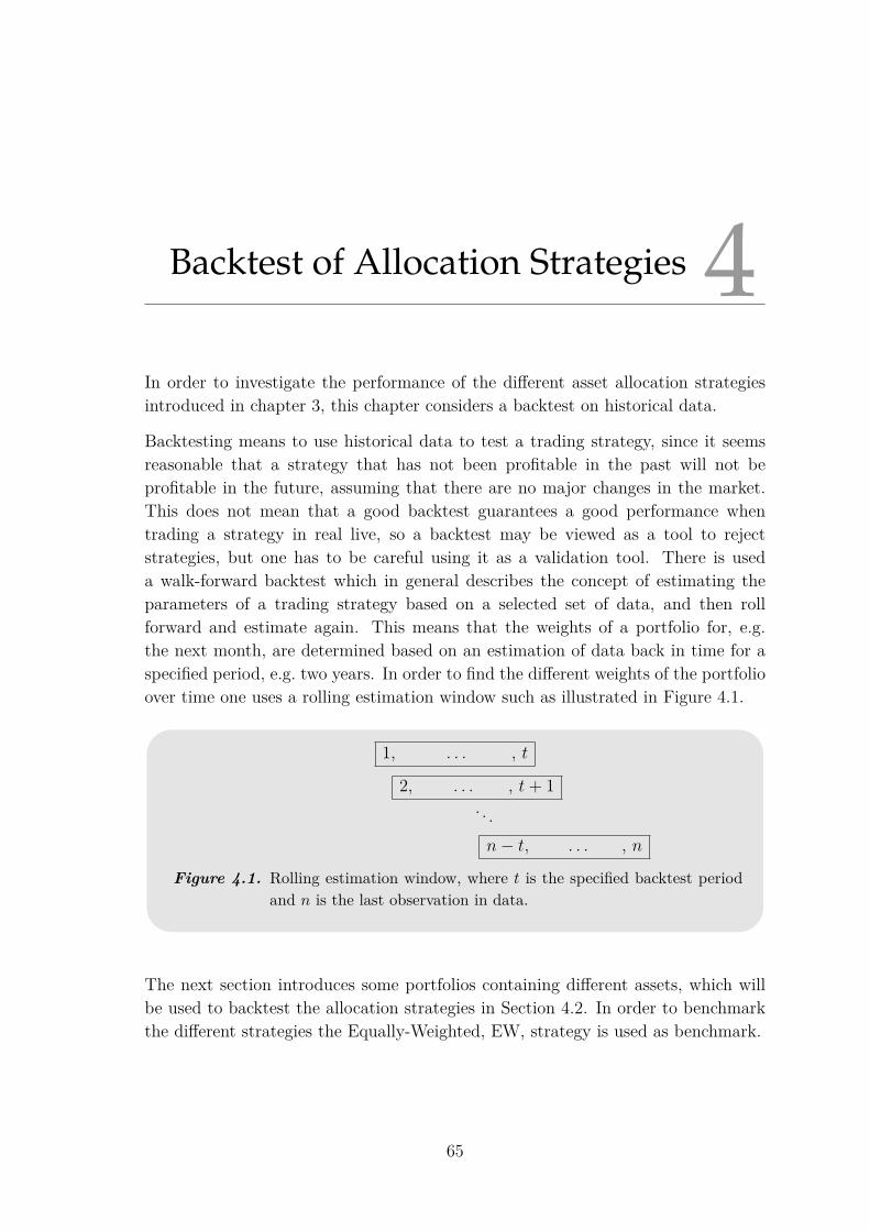
Backtest of Allocation Strategies 4In order to investigate the performance of the different asset allocation strategiesintroduced in chapter 3, this chapter considers a backtest on historical data.
Backtesting means to use historical data to test a trading strategy, since it seemsreasonable that a strategy that has not been profitable in the past will not beprofitable in the future, assuming that there are no major changes in the market.This does not mean that a good backtest guarantees a good performance whentrading a strategy in real live, so a backtest may be viewed as a tool to rejectstrategies, but one has to be careful using it as a validation tool. There is useda walk-forward backtest which in general describes the concept of estimating theparameters of a trading strategy based on a selected set of data, and then rollforward and estimate again. This means that the weights of a portfolio for, e.g.the next month, are determined based on an estimation of data back in time for aspecified period, e.g. two years. In order to find the different weights of the portfolioover time one uses a rolling estimation window such as illustrated in Figure 4.1.
1, . . . , t
2, . . . , t+ 1. . .n− t, . . . , n
Figure 4.1. Rolling estimation window, where t is the specified backtest periodand n is the last observation in data.
The next section introduces some portfolios containing different assets, which willbe used to backtest the allocation strategies in Section 4.2. In order to benchmarkthe different strategies the Equally-Weighted, EW, strategy is used as benchmark.
65
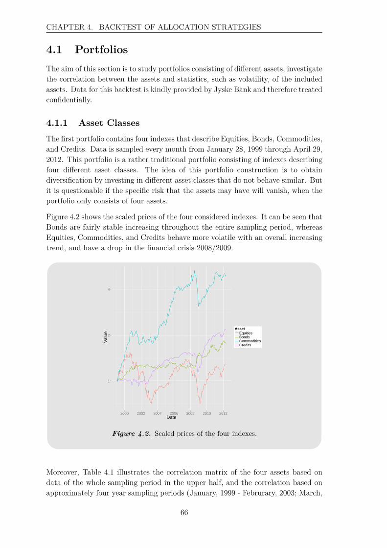
CHAPTER 4. BACKTEST OF ALLOCATION STRATEGIES
4.1 PortfoliosThe aim of this section is to study portfolios consisting of different assets, investigatethe correlation between the assets and statistics, such as volatility, of the includedassets. Data for this backtest is kindly provided by Jyske Bank and therefore treatedconfidentially.
4.1.1 Asset ClassesThe first portfolio contains four indexes that describe Equities, Bonds, Commodities,and Credits. Data is sampled every month from January 28, 1999 through April 29,2012. This portfolio is a rather traditional portfolio consisting of indexes describingfour different asset classes. The idea of this portfolio construction is to obtaindiversification by investing in different asset classes that do not behave similar. Butit is questionable if the specific risk that the assets may have will vanish, when theportfolio only consists of four assets.
Figure 4.2 shows the scaled prices of the four considered indexes. It can be seen thatBonds are fairly stable increasing throughout the entire sampling period, whereasEquities, Commodities, and Credits behave more volatile with an overall increasingtrend, and have a drop in the financial crisis 2008/2009.
1
2
4
2000 2002 2004 2006 2008 2010 2012Date
Val
ue
AssetEquitiesBondsCommoditiesCredits
Index − Portfolio Components
Figure 4.2. Scaled prices of the four indexes.
Moreover, Table 4.1 illustrates the correlation matrix of the four assets based ondata of the whole sampling period in the upper half, and the correlation based onapproximately four year sampling periods (January, 1999 - Februrary, 2003; March,
66
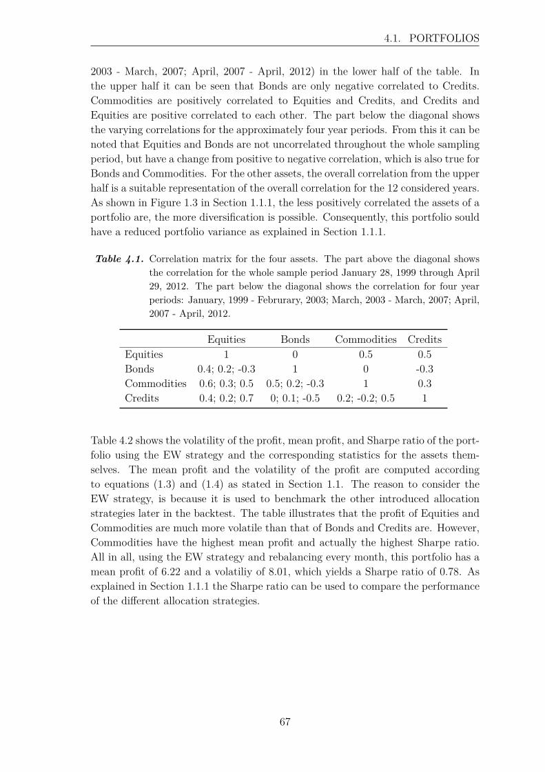
4.1. PORTFOLIOS
2003 - March, 2007; April, 2007 - April, 2012) in the lower half of the table. Inthe upper half it can be seen that Bonds are only negative correlated to Credits.Commodities are positively correlated to Equities and Credits, and Credits andEquities are positive correlated to each other. The part below the diagonal showsthe varying correlations for the approximately four year periods. From this it can benoted that Equities and Bonds are not uncorrelated throughout the whole samplingperiod, but have a change from positive to negative correlation, which is also true forBonds and Commodities. For the other assets, the overall correlation from the upperhalf is a suitable representation of the overall correlation for the 12 considered years.As shown in Figure 1.3 in Section 1.1.1, the less positively correlated the assets of aportfolio are, the more diversification is possible. Consequently, this portfolio souldhave a reduced portfolio variance as explained in Section 1.1.1.
Table 4.1. Correlation matrix for the four assets. The part above the diagonal showsthe correlation for the whole sample period January 28, 1999 through April29, 2012. The part below the diagonal shows the correlation for four yearperiods: January, 1999 - Februrary, 2003; March, 2003 - March, 2007; April,2007 - April, 2012.
Equities Bonds Commodities CreditsEquities 1 0 0.5 0.5Bonds 0.4; 0.2; -0.3 1 0 -0.3Commodities 0.6; 0.3; 0.5 0.5; 0.2; -0.3 1 0.3Credits 0.4; 0.2; 0.7 0; 0.1; -0.5 0.2; -0.2; 0.5 1
Table 4.2 shows the volatility of the profit, mean profit, and Sharpe ratio of the port-folio using the EW strategy and the corresponding statistics for the assets them-selves. The mean profit and the volatility of the profit are computed accordingto equations (1.3) and (1.4) as stated in Section 1.1. The reason to consider theEW strategy, is because it is used to benchmark the other introduced allocationstrategies later in the backtest. The table illustrates that the profit of Equities andCommodities are much more volatile than that of Bonds and Credits are. However,Commodities have the highest mean profit and actually the highest Sharpe ratio.All in all, using the EW strategy and rebalancing every month, this portfolio has amean profit of 6.22 and a volatiliy of 8.01, which yields a Sharpe ratio of 0.78. Asexplained in Section 1.1.1 the Sharpe ratio can be used to compare the performanceof the different allocation strategies.
67
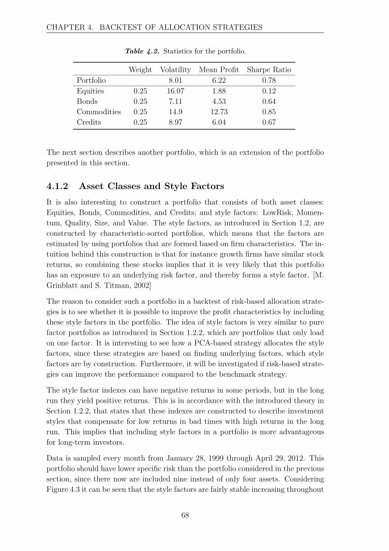
CHAPTER 4. BACKTEST OF ALLOCATION STRATEGIES
Table 4.2. Statistics for the portfolio.
Weight Volatility Mean Profit Sharpe RatioPortfolio 8.01 6.22 0.78Equities 0.25 16.07 1.88 0.12Bonds 0.25 7.11 4.53 0.64Commodities 0.25 14.9 12.73 0.85Credits 0.25 8.97 6.04 0.67
The next section describes another portfolio, which is an extension of the portfoliopresented in this section.
4.1.2 Asset Classes and Style FactorsIt is also interesting to construct a portfolio that consists of both asset classes:Equities, Bonds, Commodities, and Credits; and style factors: LowRisk, Momen-tum, Quality, Size, and Value. The style factors, as introduced in Section 1.2, areconstructed by characteristic-sorted portfolios, which means that the factors areestimated by using portfolios that are formed based on firm characteristics. The in-tuition behind this construction is that for instance growth firms have similar stockreturns, so combining these stocks implies that it is very likely that this portfoliohas an exposure to an underlying risk factor, and thereby forms a style factor. [M.Grinblatt and S. Titman, 2002]
The reason to consider such a portfolio in a backtest of risk-based allocation strate-gies is to see whether it is possible to improve the profit characteristics by includingthese style factors in the portfolio. The idea of style factors is very similar to purefactor portfolios as introduced in Section 1.2.2, which are portfolios that only loadon one factor. It is interesting to see how a PCA-based strategy allocates the stylefactors, since these strategies are based on finding underlying factors, which stylefactors are by construction. Furthermore, it will be investigated if risk-based strate-gies can improve the performance compared to the benchmark strategy.
The style factor indexes can have negative returns in some periods, but in the longrun they yield positive returns. This is in accordance with the introduced theory inSection 1.2.2, that states that these indexes are constructed to describe investmentstyles that compensate for low returns in bad times with high returns in the longrun. This implies that including style factors in a portfolio is more advantageousfor long-term investors.
Data is sampled every month from January 28, 1999 through April 29, 2012. Thisportfolio should have lower specific risk than the portfolio considered in the previoussection, since there now are included nine instead of only four assets. ConsideringFigure 4.3 it can be seen that the style factors are fairly stable increasing throughout
68
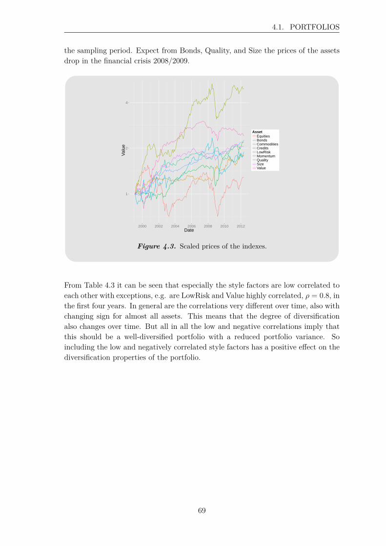
4.1. PORTFOLIOS
the sampling period. Expect from Bonds, Quality, and Size the prices of the assetsdrop in the financial crisis 2008/2009.
1
2
4
2000 2002 2004 2006 2008 2010 2012Date
Val
ue
AssetEquitiesBondsCommoditiesCreditsLowRiskMomentumQualitySizeValue
Index − Portfolio Components
Figure 4.3. Scaled prices of the indexes.
From Table 4.3 it can be seen that especially the style factors are low correlated toeach other with exceptions, e.g. are LowRisk and Value highly correlated, ρ = 0.8, inthe first four years. In general are the correlations very different over time, also withchanging sign for almost all assets. This means that the degree of diversificationalso changes over time. But all in all the low and negative correlations imply thatthis should be a well-diversified portfolio with a reduced portfolio variance. Soincluding the low and negatively correlated style factors has a positive effect on thediversification properties of the portfolio.
69
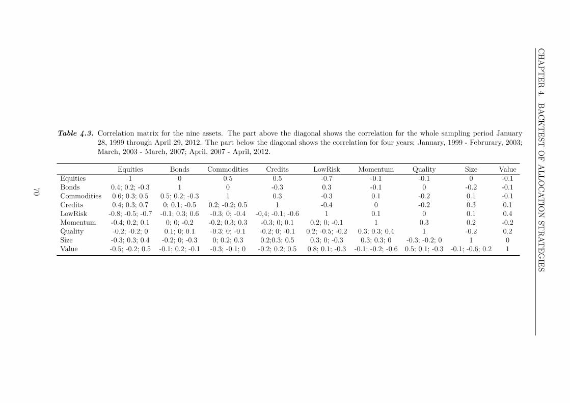
CHAPT
ER4.
BACKTEST
OFALLO
CAT
ION
STRAT
EGIES
Table 4.3. Correlation matrix for the nine assets. The part above the diagonal shows the correlation for the whole sampling period January28, 1999 through April 29, 2012. The part below the diagonal shows the correlation for four years: January, 1999 - Februrary, 2003;March, 2003 - March, 2007; April, 2007 - April, 2012.
Equities Bonds Commodities Credits LowRisk Momentum Quality Size ValueEquities 1 0 0.5 0.5 -0.7 -0.1 -0.1 0 -0.1Bonds 0.4; 0.2; -0.3 1 0 -0.3 0.3 -0.1 0 -0.2 -0.1Commodities 0.6; 0.3; 0.5 0.5; 0.2; -0.3 1 0.3 -0.3 0.1 -0.2 0.1 -0.1Credits 0.4; 0.3; 0.7 0; 0.1; -0.5 0.2; -0.2; 0.5 1 -0.4 0 -0.2 0.3 0.1LowRisk -0.8; -0.5; -0.7 -0.1; 0.3; 0.6 -0.3; 0; -0.4 -0,4; -0.1; -0.6 1 0.1 0 0.1 0.4Momentum -0.4; 0.2; 0.1 0; 0; -0.2 -0.2; 0.3; 0.3 -0.3; 0; 0.1 0.2; 0; -0.1 1 0.3 0.2 -0.2Quality -0.2; -0.2; 0 0.1; 0; 0.1 -0.3; 0; -0.1 -0.2; 0; -0.1 0.2; -0.5; -0.2 0.3; 0.3; 0.4 1 -0.2 0.2Size -0.3; 0.3; 0.4 -0.2; 0; -0.3 0; 0.2; 0.3 0.2;0.3; 0.5 0.3; 0; -0.3 0.3; 0.3; 0 -0.3; -0.2; 0 1 0Value -0.5; -0.2; 0.5 -0.1; 0.2; -0.1 -0.3; -0.1; 0 -0.2; 0.2; 0.5 0.8; 0.1; -0.3 -0.1; -0.2; -0.6 0.5; 0.1; -0.3 -0.1; -0.6; 0.2 1
70
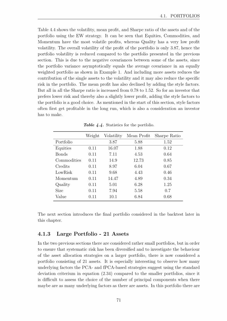
4.1. PORTFOLIOS
Table 4.4 shows the volatility, mean profit, and Sharpe ratio of the assets and of theportfolio using the EW strategy. It can be seen that Equities, Commodities, andMomentum have the most volatile profits, whereas Quality has a very low profitvolatility. The overall volatility of the profit of the portfolio is only 3.87, hence theportfolio volatility is reduced compared to the portfolio presented in the previoussection. This is due to the negative covariances between some of the assets, sincethe portfolio variance asymptotically equals the average covariance in an equallyweighted portfolio as shown in Example 1. And including more assets reduces thecontribution of the single assets to the volatility and it may also reduce the specificrisk in the portfolio. The mean profit has also declined by adding the style factors.But all in all the Sharpe ratio is increased from 0.78 to 1.52. So for an investor thatprefers lower risk and thereby also a slightly lower profit, adding the style factors tothe portfolio is a good choice. As mentioned in the start of this section, style factorsoften first get profitable in the long run, which is also a consideration an investorhas to make.
Table 4.4. Statistics for the portfolio.
Weight Volatility Mean Profit Sharpe RatioPortfolio 3.87 5.88 1.52Equities 0.11 16.07 1.88 0.12Bonds 0.11 7.11 4.53 0.64Commodities 0.11 14.9 12.73 0.85Credits 0.11 8.97 6.04 0.67LowRisk 0.11 9.68 4.43 0.46Momentum 0.11 14.47 4.89 0.34Quality 0.11 5.01 6.28 1.25Size 0.11 7.94 5.58 0.7Value 0.11 10.1 6.84 0.68
The next section introduces the final portfolio considered in the backtest later inthis chapter.
4.1.3 Large Portfolio - 21 AssetsIn the two previous sections there are considered rather small portfolios, but in orderto ensure that systematic risk has been diversified and to investigate the behaviourof the asset allocation strategies on a larger portfolio, there is now considered aportfolio consisting of 21 assets. It is especially interesting to observe how manyunderlying factors the PCA- and fPCA-based strategies suggest using the standarddeviation criterium in equation (2.34) compared to the smaller portfolios, since itis difficult to assess the choice of the number of principal components when theremaybe are as many underlying factors as there are assets. In this portfolio there are
71
CHAPTER 4. BACKTEST OF ALLOCATION STRATEGIES
included the same assets as in the previous portfolios: Equities, Bonds, Commodi-ties, Credits, LowRisk, Momentum, Quality, Size, and Value. And then there areincluded additional equity indexes representing different markets: Europe, USA,Japan, and Emerging Markets (EM); and an additional goverment bond describ-ing the 10 year interest rate in Denmark: BondsDK; and some indexes describingdifferent commodities: LiveStock, Agriculture (Agri), Precious Metal (PrecMetal),Energy, Industrial Metal (IndMetal), Oil, and Gold.
Some of the assets have different sampling rates, i.e. the equity indexes: Europe,USA, Japan, EM, and the commodity index Gold are sampled on all trading dayswhereas the other assets are sampled on a monthly basis. When combining theseassets into one portfolio there are only considered monthly observations such thatonly the observations that are in accordance with the monthly observations areconsidered. This is due to technical reason in the backtest setup. As mentionedin Chapter 2 it is possible to include all observation in the functional approach ofthe Equal Risk, ER, strategy, but this is beyond the scope of this thesis. So datais sampled every month from January 28, 1999 through April 29, 2012. Figure 4.4shows the scaled prices of the added 12 assets in this portfolio. It is observablethat some of the assets behave very similar whereas others act independently ofeach other. At the same time is the price range of the assets larger in this portfoliocompared to the two previous ones.
2
8
2000 2002 2004 2006 2008 2010 2012Date
Val
ue
AssetLiveStockAgriPrecMetalEnergyIndMetalOilGoldEuropeUSAJapanEMBondsDK
Index − Portfolio Components
Figure 4.4. The scaled prices of the added 12 assets in the portfolio are shown.The prices of the other assets can be seen in Figure 4.3.
72
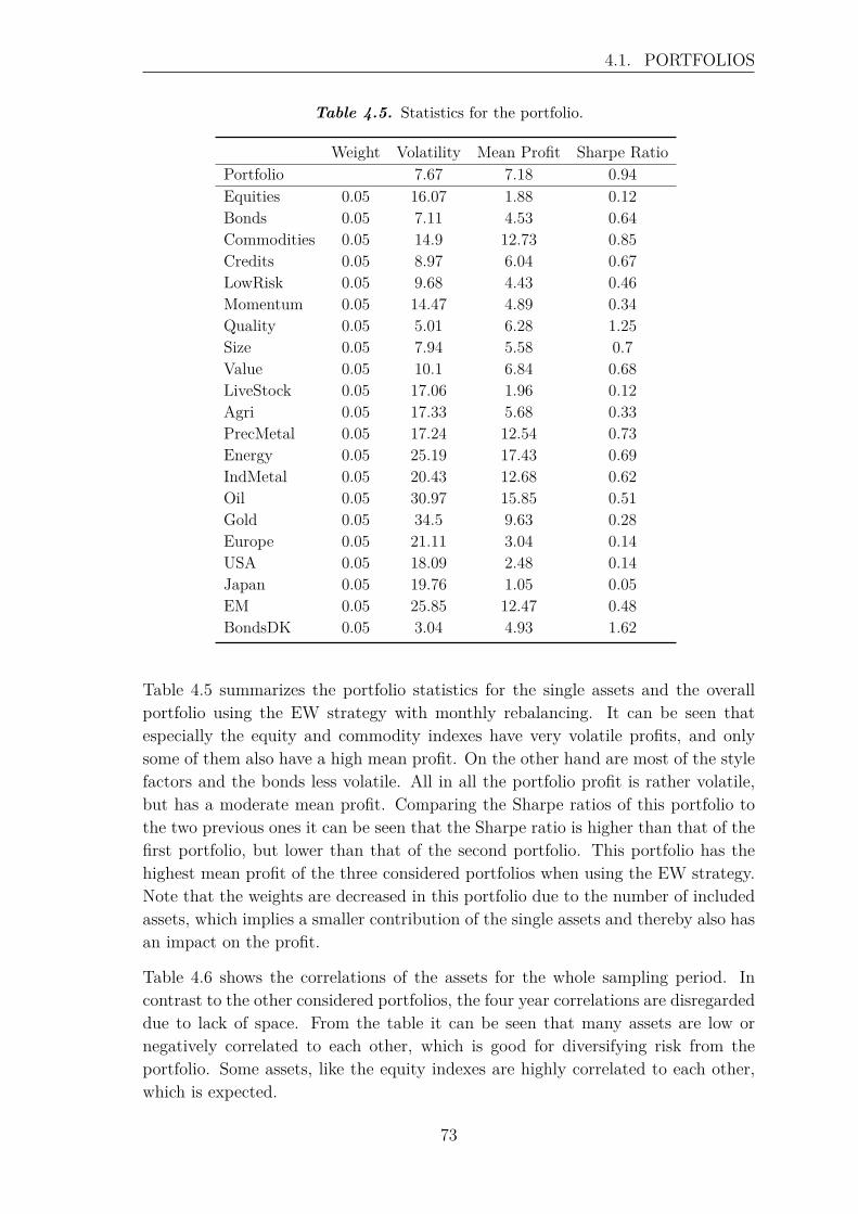
4.1. PORTFOLIOS
Table 4.5. Statistics for the portfolio.
Weight Volatility Mean Profit Sharpe RatioPortfolio 7.67 7.18 0.94Equities 0.05 16.07 1.88 0.12Bonds 0.05 7.11 4.53 0.64Commodities 0.05 14.9 12.73 0.85Credits 0.05 8.97 6.04 0.67LowRisk 0.05 9.68 4.43 0.46Momentum 0.05 14.47 4.89 0.34Quality 0.05 5.01 6.28 1.25Size 0.05 7.94 5.58 0.7Value 0.05 10.1 6.84 0.68LiveStock 0.05 17.06 1.96 0.12Agri 0.05 17.33 5.68 0.33PrecMetal 0.05 17.24 12.54 0.73Energy 0.05 25.19 17.43 0.69IndMetal 0.05 20.43 12.68 0.62Oil 0.05 30.97 15.85 0.51Gold 0.05 34.5 9.63 0.28Europe 0.05 21.11 3.04 0.14USA 0.05 18.09 2.48 0.14Japan 0.05 19.76 1.05 0.05EM 0.05 25.85 12.47 0.48BondsDK 0.05 3.04 4.93 1.62
Table 4.5 summarizes the portfolio statistics for the single assets and the overallportfolio using the EW strategy with monthly rebalancing. It can be seen thatespecially the equity and commodity indexes have very volatile profits, and onlysome of them also have a high mean profit. On the other hand are most of the stylefactors and the bonds less volatile. All in all the portfolio profit is rather volatile,but has a moderate mean profit. Comparing the Sharpe ratios of this portfolio tothe two previous ones it can be seen that the Sharpe ratio is higher than that of thefirst portfolio, but lower than that of the second portfolio. This portfolio has thehighest mean profit of the three considered portfolios when using the EW strategy.Note that the weights are decreased in this portfolio due to the number of includedassets, which implies a smaller contribution of the single assets and thereby also hasan impact on the profit.
Table 4.6 shows the correlations of the assets for the whole sampling period. Incontrast to the other considered portfolios, the four year correlations are disregardeddue to lack of space. From the table it can be seen that many assets are low ornegatively correlated to each other, which is good for diversifying risk from theportfolio. Some assets, like the equity indexes are highly correlated to each other,which is expected.
73
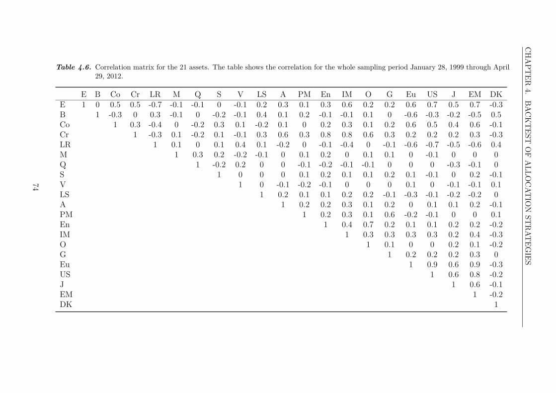
CHAPT
ER4.
BACKTEST
OFALLO
CAT
ION
STRAT
EGIES
Table 4.6. Correlation matrix for the 21 assets. The table shows the correlation for the whole sampling period January 28, 1999 through April29, 2012.
E B Co Cr LR M Q S V LS A PM En IM O G Eu US J EM DKE 1 0 0.5 0.5 -0.7 -0.1 -0.1 0 -0.1 0.2 0.3 0.1 0.3 0.6 0.2 0.2 0.6 0.7 0.5 0.7 -0.3B 1 -0.3 0 0.3 -0.1 0 -0.2 -0.1 0.4 0.1 0.2 -0.1 -0.1 0.1 0 -0.6 -0.3 -0.2 -0.5 0.5Co 1 0.3 -0.4 0 -0.2 0.3 0.1 -0.2 0.1 0 0.2 0.3 0.1 0.2 0.6 0.5 0.4 0.6 -0.1Cr 1 -0.3 0.1 -0.2 0.1 -0.1 0.3 0.6 0.3 0.8 0.8 0.6 0.3 0.2 0.2 0.2 0.3 -0.3LR 1 0.1 0 0.1 0.4 0.1 -0.2 0 -0.1 -0.4 0 -0.1 -0.6 -0.7 -0.5 -0.6 0.4M 1 0.3 0.2 -0.2 -0.1 0 0.1 0.2 0 0.1 0.1 0 -0.1 0 0 0Q 1 -0.2 0.2 0 0 -0.1 -0.2 -0.1 -0.1 0 0 0 -0.3 -0.1 0S 1 0 0 0 0.1 0.2 0.1 0.1 0.2 0.1 -0.1 0 0.2 -0.1V 1 0 -0.1 -0.2 -0.1 0 0 0 0.1 0 -0.1 -0.1 0.1LS 1 0.2 0.1 0.1 0.2 0.2 -0.1 -0.3 -0.1 -0.2 -0.2 0A 1 0.2 0.2 0.3 0.1 0.2 0 0.1 0.1 0.2 -0.1PM 1 0.2 0.3 0.1 0.6 -0.2 -0.1 0 0 0.1En 1 0.4 0.7 0.2 0.1 0.1 0.2 0.2 -0.2IM 1 0.3 0.3 0.3 0.3 0.2 0.4 -0.3O 1 0.1 0 0 0.2 0.1 -0.2G 1 0.2 0.2 0.2 0.3 0Eu 1 0.9 0.6 0.9 -0.3US 1 0.6 0.8 -0.2J 1 0.6 -0.1EM 1 -0.2DK 1
74
4.2. BACKTEST
After having introduced the different portfolios, the next section deals with investi-gating the performance of the different asset allocation strategies on historical databy among others comparing their profits, Sharpe ratios, and turnovers. Further-more, the selected portfolio weights are investigated over time.
4.2 BacktestThis section aims to examine the performance of the different risk-based alloca-tion strategies introduced in Chapter 3 compared to the benchmark strategy: EW,and the traditional MVa strategy by a walk-forward backtest on the portfolios asdescribed in Section 4.1. The considered asset allocation strategies are:
• Equally-Weighted strategy (EW):
w∗ = N−1.
• Minimum Variance strategy (MVa):
w∗ = minw
N∑i=1
N∑j=1
wiwjσij.
• Equal Risk strategy – risk contribution approach (ER - RC):
w∗ = argminw
N∑i=1
N∑j=1
(wi(Σw)i − wj(Σw)j)2 .
• Equal Risk strategy – PCA approach (ER - PCA):
w∗ = minw
m∑j=1
CPVj.
• Equal Risk strategy – fPCA approach (ER - fPCA):
w∗ = minw
m∑j=1
CPVj.
• Equal Risk strategy – PCA risk contribution approach (ER - PCA RC):
w∗ = argminw
m∑i=1
m∑j=1
(RCi − RCj
)2.
• Diversified Risk Parity strategy (DRP):
w∗ = arg maxwNH .
The reason that the MVa strategy is tested and not the Markowitz Mean-Variance,MV, strategy is due the fact that the aim of this backtest is to compare the per-formance of the alternative risk-based strategies with the benchmark strategy and
75
CHAPTER 4. BACKTEST OF ALLOCATION STRATEGIES
a traditional strategy, but the MV strategy might find completely other portfolioweights due to a high estimation error of the mean. So in order to obtain a meaning-ful comparison of the different allocation strategies the MVa strategy is considered,which is a special case of the MV strategy, and is exclusively based on the estima-tion of the covariance matrix Σ, hence it is more similar to the other consideredstrategies.
Appendix A.2 illustrates how the backtest is set up in R using a flow chart. Firstthe selected portfolio is read from a database, which then is inputted in a functionthat can perform the backtest. Data is transformed to log returns as described inequation (1.1) and outliers are detected and cut off by considering the standarddeviation of the log return of an asset in the following way:
| log(Ri(t))| > 2σi ⇒ log(Ri(t)) = ±2σi for i = 1, . . . , N,
where log(Ri(t)) is the log return of asset i at time t, σi is the standard deviationof asset i, and N is the number of assets in a portfolio. This means that valuesthat are larger in absolute value than two times the standard deviation of the con-sidered asset are cut off and set to be two times the standard deviation. Then thisfunction calls an optimization function, which is dependent on the asset allocationstrategy. Before performing the optimization some strategies need to specify someadditional parameters, e.g. the PCA-based strategies need the number of princi-pal components, which is determined by the criterium in equation (2.34). Thusthe number of principal components m, the number of basis functions K, and thesmoothing parameter λ are computed before performing the backtest, such that theused parameters are the same throughout the whole backtest period. Furthermore,the optimization methods need an initial guess for the portfolio weights, which forall strategies are set to equal weights.
Since all three portfolios introduced in Section 4.1 are modified to have a monthlysampling rate, the portfolio weights of the different strategies are rebalanced everymonth based on an estimation of the past two or five years, respectively. Therebydata from the first two or five years are exclusively used for estimation purposes. It isassumed that short-selling is not allowed, which is due to the theoretical limitationsof some of the strategies in this thesis, e.g. the ER- RC strategy. After the firstestimation of the weights, the estimated portfolio weights are used recursively asinitial weights to find the weights for the next period. This is in accordance withthe theory introduced in Section 1.1. Another possibility would be to always useequal weights as initial weights, which might result in a different allocation.
In the backtest setup transaction costs are ignored, but in order to determine howgood an asset allocation strategy performs it is also essential to know how much itwill cost to use a specific strategy. Therefore the statistic describing the averageturnover over T periods can be considered:
TO = 1T − 1
T∑t=2
N∑i=1|wi(t)− wi(t− 1)|, (4.1)
76
4.2. BACKTEST
where N is the number of assets, wi(t) is the portfolio weight of asset i at timet. The value of TO equals the average amount of buy and sell transactions as apercentage of the portfolio value. [Kind, 2013] Often a low value of TO is preferred,but if a strategy has very high profits, a high turnover might still pay off.
It is also interesting to consider the concentration of the portfolio, i.e. if some assetsare weighted much higher than others, using the different strategies over time t.One possible statistic to measure concentration is the so-called Herfindahl index,h(t), which is given by:
h(t) =N∑i=1
wi(t)2,
where wi(t) is the weight of asset i at time t. The index equals one if a portfoliois concentrated, i.e. there is only invested in one asset. On the other hand whenthere is invested uniformly in all assets then the index equals N−1. Usually thenormalized Herfindahl index, NH(t), is considered:
NH(t) = h(t)− 1/N1− 1/N ,
where NH(t) ∈ [0, 1]. In general, a low value of NH(t) is preferred, since thisindicates a balanced portfolio. [S. Maillard, T. Roncalli, J. Teiletche, 2009]
The following sections backtest the introduced asset allocation strategies on thedifferent portfolios introduced in Section 4.1. A summary of the most importantresults of the backtest can be found in Section 4.3.
4.2.1 Asset ClassesThe first backtest of the mentioned asset allocation strategies is based on the port-folio consisting of asset classes as introduced in Section 4.1.1. First a two yearestimation window is used and later in this section also a five year estimation win-dow is considered.
For the strategies based on PCA the number of principal components m is deter-mined using the standard deviation criterium from equation (2.34) with v = 0.1.This means that only components whose standard deviation is larger than 10% ofthe first principal component’s standard deviation are included in the PCA, whichis done to ensure that the included components account for enough variation andthereby represent an underlying risk factor. The choice of the parameter v is ad hocand will therefore be investigated. This is also done for the ER- fPCA strategy andin addition the smoothing parameter λ and the number of basis functions K aredetermined using cross validation as explained in Section 3.1.3. Note that since allassets have a constant sampling rate, equally spaced B-splines are used to smoothdata in the ER- fPCA strategy. The determined parameters are summarized inTable 4.7.
77
CHAPTER 4. BACKTEST OF ALLOCATION STRATEGIES
Table 4.7. The determined number of principal components m for the strategies basedon PCA and fPCA for v = 0.1. And the chosen number of basis functions Kand the smoothing paramter λ for the fPCA approach determined by crossvalidation.
Strategy m K λ
PCA-based 4 - -fPCA-based 3 15 10000
It can be seen from Table 4.7 that for the PCA-based strategies all principal compo-nents are used, whereas in the case of ER- fPCA only three principal components areused. This means that the PCA-based strategies suggest that there are four latentfactors, whereas the ER- fPCA strategy suggests three factors. The difference inthe number of principal components might be caused by smoothing data, which canremove noise and reduces the variability of data, hence the eigenvalues might alsodecrease and thereby the standard deviation criterium suggests a lower number ofprincipal components. But since this portfolio only consists of four assets, it mightbe appropriate that there are four underlying factors that drive the assets.
The scaled portfolio profits for the different strategies are displayed in Figure 4.5.The first two years are used as initial backtest period, hence the portfolio weightsare first determined from ultimo January 2001. After this period there can beobserved differences in the resulting profits of the different strategies, where it canbe noted that the ER- PCA RC and DRP outperform the benchmark strategy andthat the EW and ER- fPCA strategy drop during the financial crisis, whereas theother strategies perform quite stable.
2000 2004 2008 2012
1.0
2.0
3.0
Indexed Portfolio Profit
Date
Pro
fit
MVaEWER − PCAER − RCER − PCA RCER − fPCADRP
Figure 4.5. Scaled portfolio profits of the asset allocation strategies. The firsttwo years are exclusively used to estimate the first backtest weights.
78
4.2. BACKTEST
Figure 4.6 shows the portfolio weights over time for the different strategies. It canbe observed that the weights of the ER- RC and ER- PCA approaches are verysimilar to each other, which is consistent with the results obtained in the simulationstudy in Section 3.4. As investigated in Section 4.1.1 the correlations of the assetsin this portfolio are very similar to each other, expect from the negative correlationsof Bonds and Credits. Therefore it is expected from the results in Section 3.1 thatthe ER- RC strategy finds weights that are inversely related to the volatilites of thesingle assets. Using the volatilies from Table 4.2 it is assumed that the weights forEquities and Commodities are very similar and small, whereas the weights for Bondsand Credits are larger and on average also are very similar. This can be confirmedby the portfolio weights found in Figure 4.6. The weights of the ER- PCA RC andDRP approaches are also very similar, which also is expected from the results ofSection 3.4. The ER- fPCA strategy finds completely other weights and has a veryhigh turnover, which is disadvantageous for an asset allocation strategy since thiscan imply high transaction costs. The MVa strategy gives most weight to the leastvolatile assets, Bonds and Credits, which is in accordance with the aim of findingportfolio weights that result in the minimum portfolio variance. As expected fromthe correlation matrix in Figure 4.1, where it can be seen that Bonds and Creditsare negatively correlated, the weights for these behave reversed in all strategies, butin the case of the ER- fPCA strategy it is difficult to see this behaviour due to thehigh turnover of this strategy.
79
CHAPTER 4. BACKTEST OF ALLOCATION STRATEGIES
ER - PCA
0.0
0.2
0.4
0.6
2000 2002 2004 2006 2008 2010 2012Date
Val
ue
AssetEquitiesBondsCommoditiesCredits
Portfolio Weights ER - RC
0.2
0.4
0.6
2000 2002 2004 2006 2008 2010 2012Date
Val
ue
AssetEquitiesBondsCommoditiesCredits
Portfolio Weights
ER - PCA RC
0.0
0.2
0.4
0.6
0.8
2000 2002 2004 2006 2008 2010 2012Date
Val
ue
AssetEquitiesBondsCommoditiesCredits
Portfolio Weights ER - fPCA
0.00
0.25
0.50
0.75
1.00
2000 2002 2004 2006 2008 2010 2012Date
Val
ue
AssetEquitiesBondsCommoditiesCredits
Portfolio Weights
Diversified Risk Parity
0.00
0.25
0.50
0.75
2000 2002 2004 2006 2008 2010 2012Date
Val
ue
AssetEquitiesBondsCommoditiesCredits
Portfolio Weights Minimum Variance
0.00
0.25
0.50
0.75
1.00
2000 2002 2004 2006 2008 2010 2012Date
Val
ue
AssetEquitiesBondsCommoditiesCredits
Portfolio Weights
Figure 4.6. The weights of the different strategies estimated on a rolling windowof two years and rebalanced every month. Note that the vertical axesdiffer for some of the strategies.
80
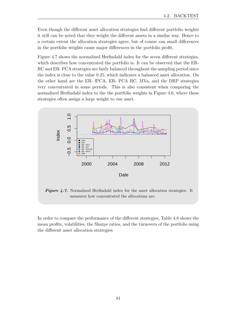
4.2. BACKTEST
Even though the different asset allocation strategies find different portfolio weightsit still can be noted that they weight the different assets in a similar way. Hence toa certain extent the allocation strategies agree, but of course can small differencesin the portfolio weights cause major differences in the portfolio profit.
Figure 4.7 shows the normalized Herfindahl index for the seven different strategies,which describes how concentrated the portfolio is. It can be observed that the ER-RC and ER- PCA strategies are fairly balanced throughout the sampling period sincethe index is close to the value 0.25, which indicates a balanced asset allocation. Onthe other hand are the ER- fPCA, ER- PCA RC, MVa, and the DRP strategiesvery concentrated in some periods. This is also consistent when comparing thenormalized Herfindahl index to the the portfolio weights in Figure 4.6, where thesestrategies often assign a large weight to one asset.
2000 2004 2008 2012
−0.
50.
00.
51.
0
Herfindahl Index
Date
Inde
x
MVaEWER − PCAER − RCER − PCA RCER − fPCADRP
Figure 4.7. Normalized Herfindahl index for the asset allocation strategies. Itmeasures how concentrated the allocations are.
In order to compare the performance of the different strategies, Table 4.8 shows themean profits, volatilities, the Sharpe ratios, and the turnovers of the portfolio usingthe different asset allocation strategies.
81
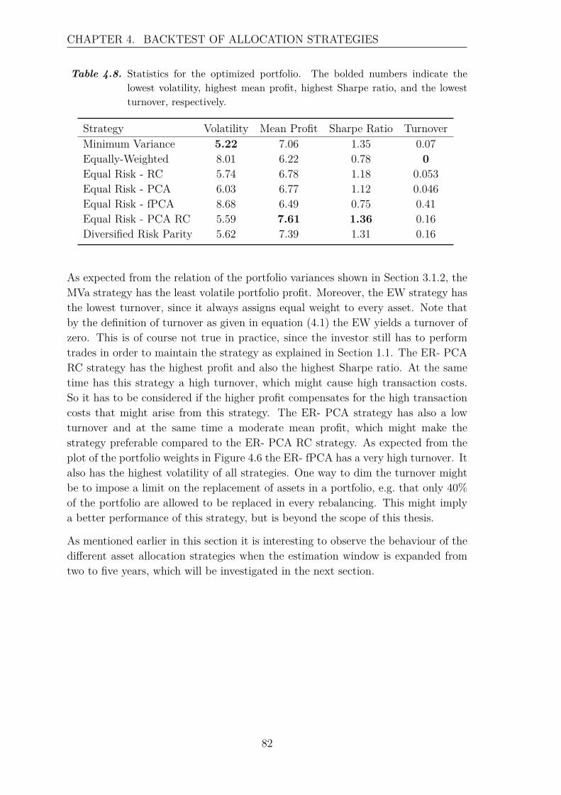
CHAPTER 4. BACKTEST OF ALLOCATION STRATEGIES
Table 4.8. Statistics for the optimized portfolio. The bolded numbers indicate thelowest volatility, highest mean profit, highest Sharpe ratio, and the lowestturnover, respectively.
Strategy Volatility Mean Profit Sharpe Ratio TurnoverMinimum Variance 5.22 7.06 1.35 0.07Equally-Weighted 8.01 6.22 0.78 0Equal Risk - RC 5.74 6.78 1.18 0.053Equal Risk - PCA 6.03 6.77 1.12 0.046Equal Risk - fPCA 8.68 6.49 0.75 0.41Equal Risk - PCA RC 5.59 7.61 1.36 0.16Diversified Risk Parity 5.62 7.39 1.31 0.16
As expected from the relation of the portfolio variances shown in Section 3.1.2, theMVa strategy has the least volatile portfolio profit. Moreover, the EW strategy hasthe lowest turnover, since it always assigns equal weight to every asset. Note thatby the definition of turnover as given in equation (4.1) the EW yields a turnover ofzero. This is of course not true in practice, since the investor still has to performtrades in order to maintain the strategy as explained in Section 1.1. The ER- PCARC strategy has the highest profit and also the highest Sharpe ratio. At the sametime has this strategy a high turnover, which might cause high transaction costs.So it has to be considered if the higher profit compensates for the high transactioncosts that might arise from this strategy. The ER- PCA strategy has also a lowturnover and at the same time a moderate mean profit, which might make thestrategy preferable compared to the ER- PCA RC strategy. As expected from theplot of the portfolio weights in Figure 4.6 the ER- fPCA has a very high turnover. Italso has the highest volatility of all strategies. One way to dim the turnover mightbe to impose a limit on the replacement of assets in a portfolio, e.g. that only 40%of the portfolio are allowed to be replaced in every rebalancing. This might implya better performance of this strategy, but is beyond the scope of this thesis.
As mentioned earlier in this section it is interesting to observe the behaviour of thedifferent asset allocation strategies when the estimation window is expanded fromtwo to five years, which will be investigated in the next section.
82
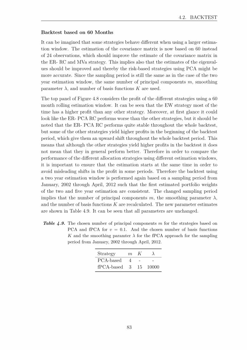
4.2. BACKTEST
Backtest based on 60 Months
It can be imagined that some strategies behave different when using a larger estima-tion window. The estimation of the covariance matrix is now based on 60 insteadof 24 observations, which should improve the estimate of the covariance matrix inthe ER- RC and MVa strategy. This implies also that the estimates of the eigenval-ues should be improved and thereby the risk-based strategies using PCA might bemore accurate. Since the sampling period is still the same as in the case of the twoyear estimation window, the same number of principal components m, smoothingparameter λ, and number of basis functions K are used.
The top panel of Figure 4.8 considers the profit of the different strategies using a 60month rolling estimation window. It can be seen that the EW strategy most of thetime has a higher profit than any other strategy. Moreover, at first glance it couldlook like the ER- PCA RC performs worse than the other strategies, but it should benoted that the ER- PCA RC performs quite stable throughout the whole backtest,but some of the other strategies yield higher profits in the beginning of the backtestperiod, which give them an upward shift throughout the whole backtest period. Thismeans that although the other strategies yield higher profits in the backtest it doesnot mean that they in general perform better. Therefore in order to compare theperformance of the different allocation strategies using different estimation windows,it is important to ensure that the estimation starts at the same time in order toavoid misleading shifts in the profit in some periods. Therefore the backtest usinga two year estimation window is performed again based on a sampling period fromJanuary, 2002 through April, 2012 such that the first estimated portfolio weightsof the two and five year estimation are consistent. The changed sampling periodimplies that the number of principal components m, the smoothing parameter λ,and the number of basis functions K are recalculated. The new parameter estimatesare shown in Table 4.9. It can be seen that all parameters are unchanged.
Table 4.9. The chosen number of principal components m for the strategies based onPCA and fPCA for v = 0.1. And the chosen number of basis functionsK and the smoothing paramter λ for the fPCA approach for the samplingperiod from January, 2002 through April, 2012.
Strategy m K λ
PCA-based 4 - -fPCA-based 3 15 10000
83
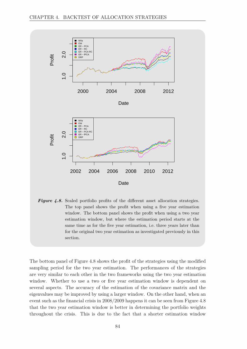
CHAPTER 4. BACKTEST OF ALLOCATION STRATEGIES
2000 2004 2008 2012
1.0
2.0
Indexed Portfolio Profit
Date
Pro
fit
MVaEWER − PCAER − RCER − PCA RCER − fPCADRP
2002 2004 2006 2008 2010 2012
1.0
2.0
Indexed Portfolio Profit
Date
Pro
fit
MVaEWER − PCAER − RCER − PCA RCER − fPCADRP
Figure 4.8. Scaled portfolio profits of the different asset allocation strategies.The top panel shows the profit when using a five year estimationwindow. The bottom panel shows the profit when using a two yearestimation window, but where the estimation period starts at thesame time as for the five year estimation, i.e. three years later thanfor the original two year estimation as investigated previously in thissection.
The bottom panel of Figure 4.8 shows the profit of the strategies using the modifiedsampling period for the two year estimation. The performances of the strategiesare very similar to each other in the two frameworks using the two year estimationwindow. Whether to use a two or five year estimation window is dependent onseveral aspects. The accuracy of the estimation of the covariance matrix and theeigenvalues may be improved by using a larger window. On the other hand, when anevent such as the financial crisis in 2008/2009 happens it can be seen from Figure 4.8that the two year estimation window is better in determining the portfolio weightsthroughout the crisis. This is due to the fact that a shorter estimation window
84
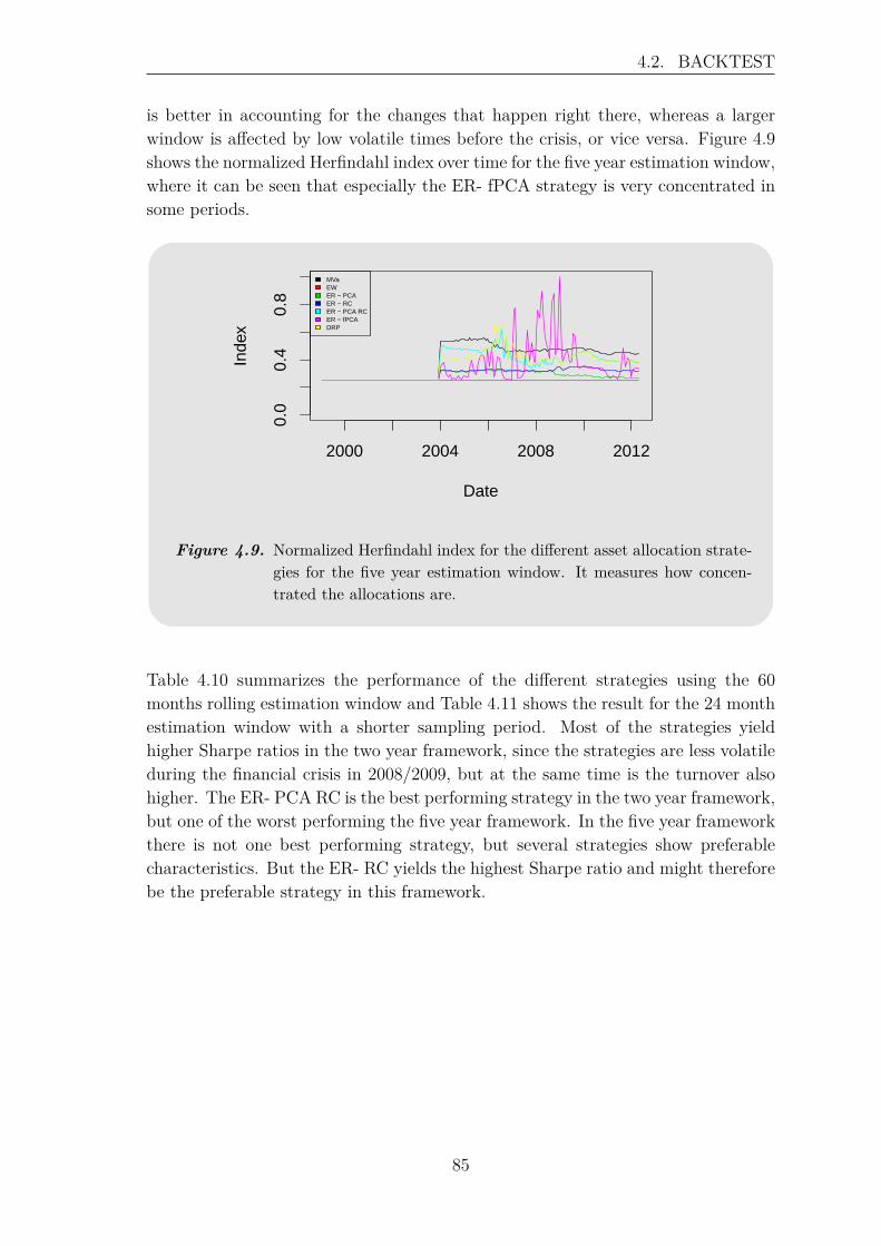
4.2. BACKTEST
is better in accounting for the changes that happen right there, whereas a largerwindow is affected by low volatile times before the crisis, or vice versa. Figure 4.9shows the normalized Herfindahl index over time for the five year estimation window,where it can be seen that especially the ER- fPCA strategy is very concentrated insome periods.
2000 2004 2008 2012
0.0
0.4
0.8
Herfindahl Index
Date
Inde
x
MVaEWER − PCAER − RCER − PCA RCER − fPCADRP
Figure 4.9. Normalized Herfindahl index for the different asset allocation strate-gies for the five year estimation window. It measures how concen-trated the allocations are.
Table 4.10 summarizes the performance of the different strategies using the 60months rolling estimation window and Table 4.11 shows the result for the 24 monthestimation window with a shorter sampling period. Most of the strategies yieldhigher Sharpe ratios in the two year framework, since the strategies are less volatileduring the financial crisis in 2008/2009, but at the same time is the turnover alsohigher. The ER- PCA RC is the best performing strategy in the two year framework,but one of the worst performing the five year framework. In the five year frameworkthere is not one best performing strategy, but several strategies show preferablecharacteristics. But the ER- RC yields the highest Sharpe ratio and might thereforebe the preferable strategy in this framework.
85
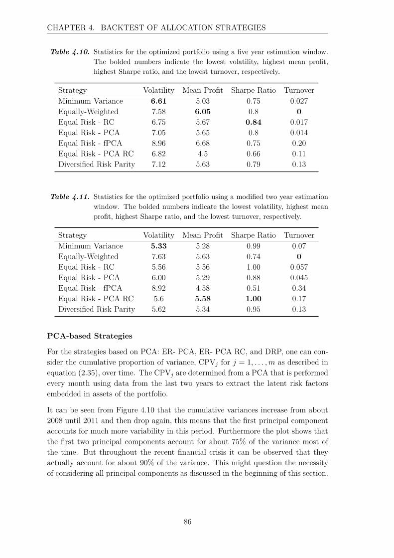
CHAPTER 4. BACKTEST OF ALLOCATION STRATEGIES
Table 4.10. Statistics for the optimized portfolio using a five year estimation window.The bolded numbers indicate the lowest volatility, highest mean profit,highest Sharpe ratio, and the lowest turnover, respectively.
Strategy Volatility Mean Profit Sharpe Ratio TurnoverMinimum Variance 6.61 5.03 0.75 0.027Equally-Weighted 7.58 6.05 0.8 0Equal Risk - RC 6.75 5.67 0.84 0.017Equal Risk - PCA 7.05 5.65 0.8 0.014Equal Risk - fPCA 8.96 6.68 0.75 0.20Equal Risk - PCA RC 6.82 4.5 0.66 0.11Diversified Risk Parity 7.12 5.63 0.79 0.13
Table 4.11. Statistics for the optimized portfolio using a modified two year estimationwindow. The bolded numbers indicate the lowest volatility, highest meanprofit, highest Sharpe ratio, and the lowest turnover, respectively.
Strategy Volatility Mean Profit Sharpe Ratio TurnoverMinimum Variance 5.33 5.28 0.99 0.07Equally-Weighted 7.63 5.63 0.74 0Equal Risk - RC 5.56 5.56 1.00 0.057Equal Risk - PCA 6.00 5.29 0.88 0.045Equal Risk - fPCA 8.92 4.58 0.51 0.34Equal Risk - PCA RC 5.6 5.58 1.00 0.17Diversified Risk Parity 5.62 5.34 0.95 0.13
PCA-based Strategies
For the strategies based on PCA: ER- PCA, ER- PCA RC, and DRP, one can con-sider the cumulative proportion of variance, CPVj for j = 1, . . . ,m as described inequation (2.35), over time. The CPVj are determined from a PCA that is performedevery month using data from the last two years to extract the latent risk factorsembedded in assets of the portfolio.
It can be seen from Figure 4.10 that the cumulative variances increase from about2008 until 2011 and then drop again, this means that the first principal componentaccounts for much more variability in this period. Furthermore the plot shows thatthe first two principal components account for about 75% of the variance most ofthe time. But throughout the recent financial crisis it can be observed that theyactually account for about 90% of the variance. This might question the necessityof considering all principal components as discussed in the beginning of this section.
86
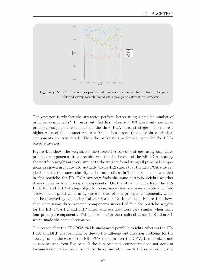
4.2. BACKTEST
0.00
0.25
0.50
0.75
1.00
2000 2002 2004 2006 2008 2010 2012Date
Val
ue
ComponentPC1PC2PC3PC4
Cumulative Variance in PCA Components
Figure 4.10. Cumulative proportion of variance extracted from the PCAs per-formed every month based on a two year estimation window.
The question is whether the strategies perform better using a smaller number ofprincipal components? It turns out that first when v > 0.3 there only are threeprincipal components considered in the three PCA-based strategies. Therefore ahigher value of the parameter v, v = 0.4, is chosen such that only three principalcomponents are considered. Then the backtest is performed again for the PCA-based strategies.
Figure 4.11 shows the weights for the three PCA-based strategies using only threeprincipal components. It can be observed that in the case of the ER- PCA strategythe portfolio weights are very similar to the weights found using all principal compo-nents as shown in Figure 4.6. Actually, Table 4.12 shows that the ER- PCA strategyyields exactly the same volatility and mean profit as in Table 4.8. This means thatin this portfolio the ER- PCA strategy finds the same portfolio weights whetherit uses three or four principal components. On the other hand perform the ER-PCA RC and DRP strategy slightly worse, since they are more volatile and yielda lower mean profit when using three instead of four principal components, whichcan be observed by comparing Tables 4.8 and 4.12. In addition, Figure 4.11 showsthat when using three principal components instead of four the portfolio weightsfor the ER- PCA RC and DRP differ, whereas they were very similar when usingfour principal components. This conforms with the results obtained in Section 3.4,which made the same observation.
The reason that the ER- PCA yields unchanged portfolio weights, whereas the ER-PCA and DRP change might be due to the different optimization problems for thestrategies. In the case of the ER- PCA the sum over the CPVj is minimized andas can be seen from Figure 4.10 the last principal component does not accountfor much cumulative variance, hence the optimization yields the same result using
87
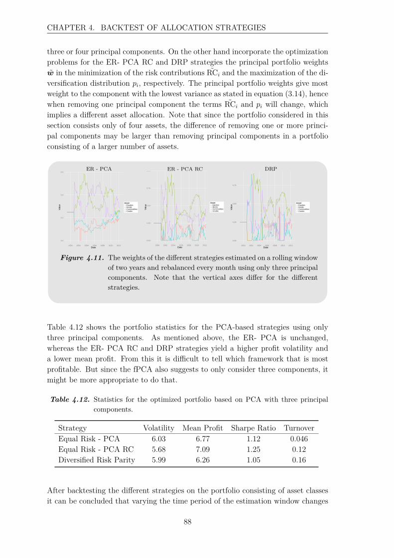
CHAPTER 4. BACKTEST OF ALLOCATION STRATEGIES
three or four principal components. On the other hand incorporate the optimizationproblems for the ER- PCA RC and DRP strategies the principal portfolio weightsw in the minimization of the risk contributions RCi and the maximization of the di-versification distribution pi, respectively. The principal portfolio weights give mostweight to the component with the lowest variance as stated in equation (3.14), hencewhen removing one principal component the terms RCi and pi will change, whichimplies a different asset allocation. Note that since the portfolio considered in thissection consists only of four assets, the difference of removing one or more princi-pal components may be larger than removing principal components in a portfolioconsisting of a larger number of assets.
ER - PCA
0.0
0.2
0.4
0.6
2000 2002 2004 2006 2008 2010 2012Date
Val
ue
AssetEquitiesBondsCommoditiesCredits
Portfolio Weights ER - PCA RC
0.00
0.25
0.50
0.75
1.00
2000 2002 2004 2006 2008 2010 2012Date
Val
ue
AssetEquitiesBondsCommoditiesCredits
Portfolio Weights DRP
0.00
0.25
0.50
0.75
2000 2002 2004 2006 2008 2010 2012Date
Val
ue
AssetEquitiesBondsCommoditiesCredits
Portfolio Weights
Figure 4.11. The weights of the different strategies estimated on a rolling windowof two years and rebalanced every month using only three principalcomponents. Note that the vertical axes differ for the differentstrategies.
Table 4.12 shows the portfolio statistics for the PCA-based strategies using onlythree principal components. As mentioned above, the ER- PCA is unchanged,whereas the ER- PCA RC and DRP strategies yield a higher profit volatility anda lower mean profit. From this it is difficult to tell which framework that is mostprofitable. But since the fPCA also suggests to only consider three components, itmight be more appropriate to do that.
Table 4.12. Statistics for the optimized portfolio based on PCA with three principalcomponents.
Strategy Volatility Mean Profit Sharpe Ratio TurnoverEqual Risk - PCA 6.03 6.77 1.12 0.046Equal Risk - PCA RC 5.68 7.09 1.25 0.12Diversified Risk Parity 5.99 6.26 1.05 0.16
After backtesting the different strategies on the portfolio consisting of asset classesit can be concluded that varying the time period of the estimation window changes
88
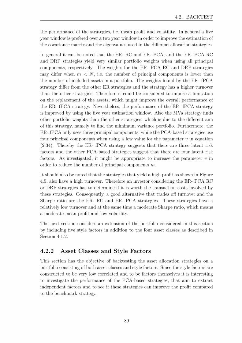
4.2. BACKTEST
the performance of the strategies, i.e. mean profit and volatility. In general a fiveyear window is prefered over a two year window in order to improve the estimation ofthe covariance matrix and the eigenvalues used in the different allocation strategies.
In general it can be noted that the ER- RC and ER- PCA, and the ER- PCA RCand DRP strategies yield very similar portfolio weights when using all principalcomponents, respectively. The weights for the ER- PCA RC and DRP strategiesmay differ when m < N , i.e. the number of principal components is lower thanthe number of included assets in a portfolio. The weights found by the ER- fPCAstrategy differ from the other ER strategies and the strategy has a higher turnoverthan the other strategies. Therefore it could be considered to impose a limitationon the replacement of the assets, which might improve the overall performance ofthe ER- fPCA strategy. Nevertheless, the performance of the ER- fPCA strategyis improved by using the five year estimation window. Also the MVa strategy findsother portfolio weights than the other strategies, which is due to the different aimof this strategy, namely to find the mimimum variance portfolio. Furthermore, theER- fPCA only uses three principal components, while the PCA-based strategies usefour principal components when using a low value for the parameter v in equation(2.34). Thereby the ER- fPCA strategy suggests that there are three latent riskfactors and the other PCA-based strategies suggest that there are four latent riskfactors. As investigated, it might be appropriate to increase the parameter v inorder to reduce the number of principal components m.
It should also be noted that the strategies that yield a high profit as shown in Figure4.5, also have a high turnover. Therefore an investor considering the ER- PCA RCor DRP strategies has to determine if it is worth the transaction costs involved bythese strategies. Consequently, a good alternative that trades off turnover and theSharpe ratio are the ER- RC and ER- PCA strategies. These strategies have arelatively low turnover and at the same time a moderate Sharpe ratio, which meansa moderate mean profit and low volatility.
The next section considers an extension of the portfolio considered in this sectionby including five style factors in addition to the four asset classes as described inSection 4.1.2.
4.2.2 Asset Classes and Style FactorsThis section has the objective of backtesting the asset allocation strategies on aportfolio consisting of both asset classes and style factors. Since the style factors areconstructed to be very low correlated and to be factors themselves it is interestingto investigate the performance of the PCA-based strategies, that aim to extractindependent factors and to see if these strategies can improve the profit comparedto the benchmark strategy.
89
CHAPTER 4. BACKTEST OF ALLOCATION STRATEGIES
The setup of the backtest in this section is inspired by the results of the previoussection. This means that both a two and five year rolling estimation window isconsidered, but such that the estimation of the portfolio weights of the two differentwindow sizes starts at the same time. This means that the backtest using thetwo year estimation window is based on the sampling period from January, 2002through April, 2012, whereas the sampling period for the five year estimation windowis from January, 1999 through April, 2012. Furthermore the parameter v in thestandard deviation criterium for determining the number of principal components isincreased from 0.1 to 0.3. The reason for this choice is to ensure that the consideredrisk factors are explanatory underlying drivers of the assets and is based on theexperiences of the previous section. Nevertheless, the profit statistics for the PCA-based strategies will also be determined using all principal components in order toinvestigate the differences of omitting components and including all components.But it is maintained that the figures of the scaled profits and the Herfindahl indexonly are considered for the PCA- and fPCA-based strategies making use of thestandard deviation criterium, since it is assumed in this thesis that there have notto be as many underlying risk factors as there are assets in a portfolio. Nevertheless,it is investigated if including the same number of principal components as there areasset makes a difference in the ER- fPCA strategy. The result is that there is nodifference in neither portfolios and therefore these results are disregarded.
This implies that the number of principal components m, the number of basis func-tionsK, and the smoothing paramter λ are determined for the two different samplingperiods and might be different. The determined parameters can be seen in Table4.13, where it can be seen that m is identical for the fPCA-based strategy for thetwo and five year estimation window. On the other hand, m differs in the case ofthe PCA-based strategies. The number of basis functions differs in the two frame-works, whereas smoothing parameter is identical. So in the two year frameworkthere are used 5 additional basis functions, which is explainable by the variation indata, which is larger considering the modified two sampling period, hence there areneeded more basis functions to better cover these variations.
Table 4.13. The chosen number of principal componentsm for strategies based on PCAand fPCA for v = 0.3. And the chosen number of basis functions K andthe smoothing paramter λ for the fPCA approach. The parameters aredisplayed for ’two year estimation winodow/ five year estimation winodow’.
Strategy m K λ
PCA-based 5/6 - -fPCA-based 4/4 15/10 10000/10000
Figure 4.12 shows the CPVj over time for the performed PCAs based on an esti-mation every month on a two year estimation window, shown in the left panel, anda five year estimation window, shown in the right panel. This figure is especially
90
4.2. BACKTEST
interesting in connection with the ER- PCA strategy, which aims to minimize theCPVj for j = 1, . . . ,m. It is observable that the CPVj’s have different paths overtime for the two different estimation windows. It is especially interesting to examinethe different behaviour during the financial crisis, where in the five year frameworkthere is a drop, which means that there are needed more principal components todescribe the same variance, whereas in the two year framework the CPVj is rising.This means that depending on which estimation window that is used, the exposureof the assets in the portfolio is rising for some risk factors in the five year frameworkand falling in the two year framework. The shorter estimation window should bebetter to capture the dynamics, i.e. the latent risk factors, that affect the assetsto a specific time since it only examines the dynamics within the past two years.Based on intuition it seems reasonable that during a financial crisis, there mightarise additional risk from factors that did not affect the assets that much duringnormal times, e.g. assets may have a much higher exposure to the volatility riskfactor.
0.00
0.25
0.50
0.75
1.00
2002 2004 2006 2008 2010 2012Date
Val
ue
ComponentPC1PC2PC3PC4PC5PC6PC7PC8PC9
Cumulative Variance in PCA Components
0.00
0.25
0.50
0.75
1.00
2000 2002 2004 2006 2008 2010 2012Date
Val
ue
ComponentPC1PC2PC3PC4PC5PC6PC7PC8PC9
Cumulative Variance in PCA Components
Figure 4.12. Cumulative proportion of variance extracted from the PCAs per-formed every month on a two year estimation window (left panel)and a five year estimation window (right panel).
The differing exposure to the latent risk factors when using the different estimationwindows must imply that the ER- PCA strategy finds different portfolio weights inthe two frameworks, which also was the case for the portfolio considered in the pre-vious section since the profits differed. This can be investigated by looking at Figure4.13, where the left panel shows the weights found in the two year framework andthe right panel shows the portfolio weights determined in the five year framework.As expected from the above discussion, the portfolio weights differ.
91
CHAPTER 4. BACKTEST OF ALLOCATION STRATEGIES
ER- PCA 24 month
0.0
0.1
0.2
0.3
2002 2004 2006 2008 2010 2012Date
Val
ue
AssetEquitiesBondsCommoditiesCreditsLowRiskMomQualitySizeValue
Portfolio Weights ER- PCA 60 month
0.0
0.1
0.2
2000 2002 2004 2006 2008 2010 2012Date
Val
ue
AssetEquitiesBondsCommoditiesCreditsLowRiskMomQualitySizeValue
Portfolio Weights
Figure 4.13. The weights of the ER- PCA strategy using a 24 month (left panel)and 60 month (right panel) estimation window, respectively. Notethat there are varying vertical axes.
In order to get an idea of how the portfolio weights of the other strategies look likeand how diversified the portfolio is during the backtest, the normalized Herfindahlindex is inspected. Figure 4.14 shows the index for the two year estimation in thetop panel and for the five year estimation window in the bottom panel. For the twoyear estimation window it is especially the MVa strategy that is concentrated mostof the time, but gets less concentrated in the end of the backtest period. The DRPand ER- fPCA strategies are concentrated in some periods, but well-diversified mostof the time. In the five year framework it is again the MVa and the DRP strategiesthat are concentrated, but also the ER- PCA RC strategy is likely to allocate muchweight to one asset. It can be concluded that especially the MVa and DRP strategiesthat often are concentrated in both estimation frameworks and at the same timethese strategies have a high turnover, which can be seen in Tables 4.14 and 4.14.
92
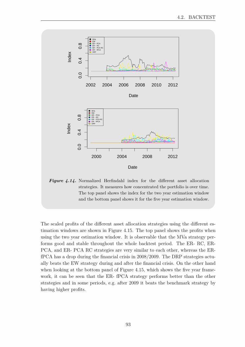
4.2. BACKTEST
2002 2004 2006 2008 2010 20120.
00.
40.
8
Herfindahl Index
Date
Inde
x
MVaEWER − PCAER − RCER − PCA RCER − fPCADRP
2000 2004 2008 2012
0.0
0.4
0.8
Herfindahl Index
Date
Inde
x
MVaEWER − PCAER − RCER − PCA RCER − fPCADRP
Figure 4.14. Normalized Herfindahl index for the different asset allocationstrategies. It measures how concentrated the portfolio is over time.The top panel shows the index for the two year estimation windowand the bottom panel shows it for the five year estimation window.
The scaled profits of the different asset allocation strategies using the different es-timation windows are shown in Figure 4.15. The top panel shows the profits whenusing the two year estimation window. It is observable that the MVa strategy per-forms good and stable throughout the whole backtest period. The ER- RC, ER-PCA, and ER- PCA RC strategies are very similar to each other, whereas the ER-fPCA has a drop during the financial crisis in 2008/2009. The DRP strategies actu-ally beats the EW strategy during and after the financial crisis. On the other handwhen looking at the bottom panel of Figure 4.15, which shows the five year frame-work, it can be seen that the ER- fPCA strategy performs better than the otherstrategies and in some periods, e.g. after 2009 it beats the benchmark strategy byhaving higher profits.
93
CHAPTER 4. BACKTEST OF ALLOCATION STRATEGIES
2002 2004 2006 2008 2010 2012
1.0
2.0
Indexed Portfolio Profit
Date
Pro
fit
MVaEWER − PCAER − RCER − PCA RCER − fPCADRP
2000 2004 2008 2012
1.0
2.0
Indexed Portfolio Profit
Date
Pro
fit
MVaEWER − PCAER − RCER − PCA RCER − fPCADRP
Figure 4.15. Scaled portfolio profits of the different asset allocation strategies.The top panel shows the profit when using a two year estimationwindow. The bottom panel shows the profit when using a five yearestimation window.
Table 4.14 shows the backtest statistics for the different allocation strategies usingthe two year estimation window. It can be seen that the DRP strategy has thehighest mean profit and at the same time the highest turnover. The MVa has thelowest volatility and the highest Sharpe ratio. Using all principal components inthe PCA-based strategies lowers the volatility of the profit, but for the ER- PCARC and DRP strategies it also lowers the mean profit and increases the turnover.Therefore it is concluded that the omitting four principal components is reasonablefor the PCA-based strategies.
94
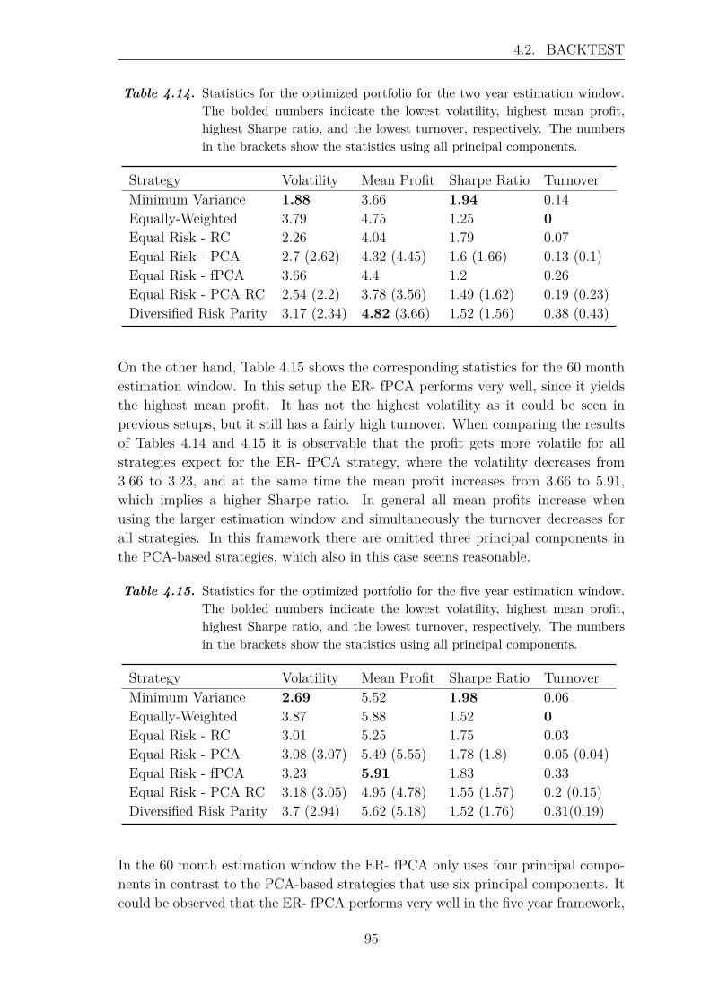
4.2. BACKTEST
Table 4.14. Statistics for the optimized portfolio for the two year estimation window.The bolded numbers indicate the lowest volatility, highest mean profit,highest Sharpe ratio, and the lowest turnover, respectively. The numbersin the brackets show the statistics using all principal components.
Strategy Volatility Mean Profit Sharpe Ratio TurnoverMinimum Variance 1.88 3.66 1.94 0.14Equally-Weighted 3.79 4.75 1.25 0Equal Risk - RC 2.26 4.04 1.79 0.07Equal Risk - PCA 2.7 (2.62) 4.32 (4.45) 1.6 (1.66) 0.13 (0.1)Equal Risk - fPCA 3.66 4.4 1.2 0.26Equal Risk - PCA RC 2.54 (2.2) 3.78 (3.56) 1.49 (1.62) 0.19 (0.23)Diversified Risk Parity 3.17 (2.34) 4.82 (3.66) 1.52 (1.56) 0.38 (0.43)
On the other hand, Table 4.15 shows the corresponding statistics for the 60 monthestimation window. In this setup the ER- fPCA performs very well, since it yieldsthe highest mean profit. It has not the highest volatility as it could be seen inprevious setups, but it still has a fairly high turnover. When comparing the resultsof Tables 4.14 and 4.15 it is observable that the profit gets more volatile for allstrategies expect for the ER- fPCA strategy, where the volatility decreases from3.66 to 3.23, and at the same time the mean profit increases from 3.66 to 5.91,which implies a higher Sharpe ratio. In general all mean profits increase whenusing the larger estimation window and simultaneously the turnover decreases forall strategies. In this framework there are omitted three principal components inthe PCA-based strategies, which also in this case seems reasonable.
Table 4.15. Statistics for the optimized portfolio for the five year estimation window.The bolded numbers indicate the lowest volatility, highest mean profit,highest Sharpe ratio, and the lowest turnover, respectively. The numbersin the brackets show the statistics using all principal components.
Strategy Volatility Mean Profit Sharpe Ratio TurnoverMinimum Variance 2.69 5.52 1.98 0.06Equally-Weighted 3.87 5.88 1.52 0Equal Risk - RC 3.01 5.25 1.75 0.03Equal Risk - PCA 3.08 (3.07) 5.49 (5.55) 1.78 (1.8) 0.05 (0.04)Equal Risk - fPCA 3.23 5.91 1.83 0.33Equal Risk - PCA RC 3.18 (3.05) 4.95 (4.78) 1.55 (1.57) 0.2 (0.15)Diversified Risk Parity 3.7 (2.94) 5.62 (5.18) 1.52 (1.76) 0.31(0.19)
In the 60 month estimation window the ER- fPCA only uses four principal compo-nents in contrast to the PCA-based strategies that use six principal components. Itcould be observed that the ER- fPCA performs very well in the five year framework,
95
CHAPTER 4. BACKTEST OF ALLOCATION STRATEGIES
which might be explainable by the fact that the ER- fPCA focuses on only four la-tent risk factors, which seems reasonable when examining the right panel of Figure4.12, since the first four principal components explain about 80% of the variancealmost during the whole backtest period.
As mentioned in the beginning of this section the motive of adding style factors to theportfolio was to investigate the allocation process of the risk-based strategies, sincestyle factors themselves represent risk factors. And indeed there can be observeda different allocation behaviour compared to the portfolio only consisting of assetclasses. Mainly, the volatility of the profit is decreased for all strategies. This meansthat adding the style factors to the portfolio makes the portfolio profits much morestable performing, which is an attractive property for many investors.
4.2.3 Large Portfolio - 21 AssetsThe last portfolio considered in the backtest of the different asset allocation strate-gies consists of 21 assets as introduced in Section 4.1.3. The reason to consider alarger portfolio is in order to investigate the behaviour of especially the PCA- andfPCA-based strategies, since it is interesting to see how many principal components,i.e. how many underlying risk factors, will be considered using a larger portfolio andhow these strategies perform compared to the strategies that solely are based onthe estimation of the covariance matrix.
There is similar to the previous sections considered a backtest with a two yearestimation window, starting from January, 2002, and a five year estimation windowusing the whole sampling period. Table 4.16 shows the chosen number of principalcomponents using v = 0.3, the number of basis functions K, and the smoothingparameter λ for the ER- fPCA strategy for the different estimation windows. It isinteresting to see that λ has the same value for both estimation windows, whereasthe number of basis functions differs. This was also the case in the previous section,but there were needed more basis functions in the two year framework, whereas hereit is in the five year framework. Similar to the previous backtests the fPCA uses lessprincipal components. So in the portfolio consisting of the 21 assets, the PCA-basedstrategies suggest that there are six or seven latent risk factors driving the assets,whereas the fPCA-based strategy suggests that there only are four latent factors.Note that similar to the previous section the statistics when using all principalcomponents in the PCA-based strategies are displayed in brackets.
96
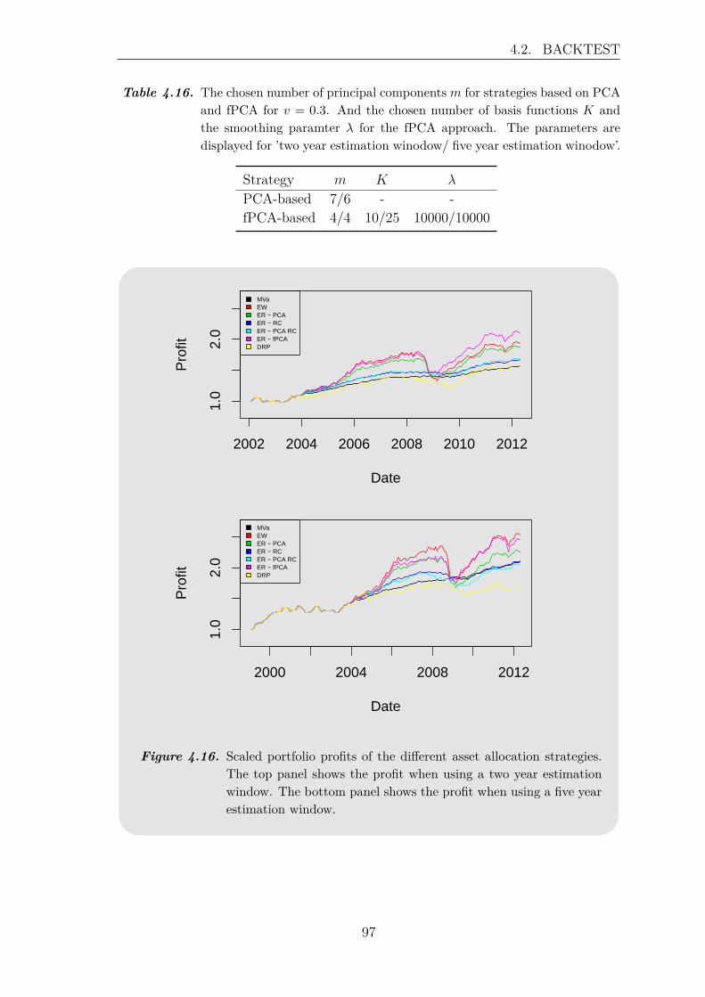
4.2. BACKTEST
Table 4.16. The chosen number of principal componentsm for strategies based on PCAand fPCA for v = 0.3. And the chosen number of basis functions K andthe smoothing paramter λ for the fPCA approach. The parameters aredisplayed for ’two year estimation winodow/ five year estimation winodow’.
Strategy m K λ
PCA-based 7/6 - -fPCA-based 4/4 10/25 10000/10000
2002 2004 2006 2008 2010 2012
1.0
2.0
Indexed Portfolio Profit
Date
Pro
fit
MVaEWER − PCAER − RCER − PCA RCER − fPCADRP
2000 2004 2008 2012
1.0
2.0
Indexed Portfolio Profit
Date
Pro
fit
MVaEWER − PCAER − RCER − PCA RCER − fPCADRP
Figure 4.16. Scaled portfolio profits of the different asset allocation strategies.The top panel shows the profit when using a two year estimationwindow. The bottom panel shows the profit when using a five yearestimation window.
97
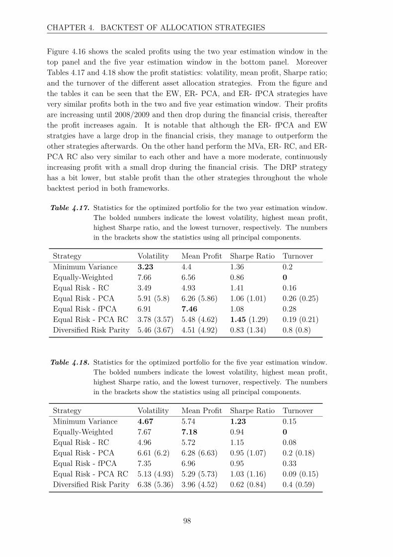
CHAPTER 4. BACKTEST OF ALLOCATION STRATEGIES
Figure 4.16 shows the scaled profits using the two year estimation window in thetop panel and the five year estimation window in the bottom panel. MoreoverTables 4.17 and 4.18 show the profit statistics: volatility, mean profit, Sharpe ratio;and the turnover of the different asset allocation strategies. From the figure andthe tables it can be seen that the EW, ER- PCA, and ER- fPCA strategies havevery similar profits both in the two and five year estimation window. Their profitsare increasing until 2008/2009 and then drop during the financial crisis, thereafterthe profit increases again. It is notable that although the ER- fPCA and EWstratgies have a large drop in the financial crisis, they manage to outperform theother strategies afterwards. On the other hand perform the MVa, ER- RC, and ER-PCA RC also very similar to each other and have a more moderate, continuouslyincreasing profit with a small drop during the financial crisis. The DRP strategyhas a bit lower, but stable profit than the other strategies throughout the wholebacktest period in both frameworks.
Table 4.17. Statistics for the optimized portfolio for the two year estimation window.The bolded numbers indicate the lowest volatility, highest mean profit,highest Sharpe ratio, and the lowest turnover, respectively. The numbersin the brackets show the statistics using all principal components.
Strategy Volatility Mean Profit Sharpe Ratio TurnoverMinimum Variance 3.23 4.4 1.36 0.2Equally-Weighted 7.66 6.56 0.86 0Equal Risk - RC 3.49 4.93 1.41 0.16Equal Risk - PCA 5.91 (5.8) 6.26 (5.86) 1.06 (1.01) 0.26 (0.25)Equal Risk - fPCA 6.91 7.46 1.08 0.28Equal Risk - PCA RC 3.78 (3.57) 5.48 (4.62) 1.45 (1.29) 0.19 (0.21)Diversified Risk Parity 5.46 (3.67) 4.51 (4.92) 0.83 (1.34) 0.8 (0.8)
Table 4.18. Statistics for the optimized portfolio for the five year estimation window.The bolded numbers indicate the lowest volatility, highest mean profit,highest Sharpe ratio, and the lowest turnover, respectively. The numbersin the brackets show the statistics using all principal components.
Strategy Volatility Mean Profit Sharpe Ratio TurnoverMinimum Variance 4.67 5.74 1.23 0.15Equally-Weighted 7.67 7.18 0.94 0Equal Risk - RC 4.96 5.72 1.15 0.08Equal Risk - PCA 6.61 (6.2) 6.28 (6.63) 0.95 (1.07) 0.2 (0.18)Equal Risk - fPCA 7.35 6.96 0.95 0.33Equal Risk - PCA RC 5.13 (4.93) 5.29 (5.73) 1.03 (1.16) 0.09 (0.15)Diversified Risk Parity 6.38 (5.36) 3.96 (4.52) 0.62 (0.84) 0.4 (0.59)
98
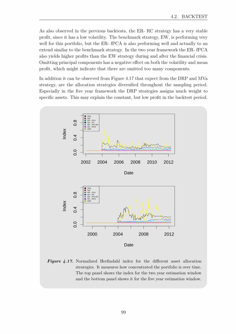
4.2. BACKTEST
As also observed in the previous backtests, the ER- RC strategy has a very stableprofit, since it has a low volatility. The benchmark strategy, EW, is performing verywell for this portfolio, but the ER- fPCA is also performing well and actually to anextend similar to the benchmark strategy. In the two year framework the ER- fPCAalso yields higher profits than the EW strategy during and after the financial crisis.Omitting principal components has a negative effect on both the volatility and meanprofit, which might indicate that there are omitted too many components.
In addition it can be observed from Figure 4.17 that expect from the DRP and MVastrategy, are the allocation strategies diversified throughout the sampling period.Especially in the five year framework the DRP strategies assigns much weight tospecific assets. This may explain the constant, but low profit in the backtest period.
2002 2004 2006 2008 2010 2012
0.0
0.4
0.8
Herfindahl Index
Date
Inde
x
MVaEWER − PCAER − RCER − PCA RCER − fPCADRP
2000 2004 2008 2012
0.0
0.4
0.8
Herfindahl Index
Date
Inde
x
MVaEWER − PCAER − RCER − PCA RCER − fPCADRP
Figure 4.17. Normalized Herfindahl index for the different asset allocationstrategies. It measures how concentrated the portfolio is over time.The top panel shows the index for the two year estimation windowand the bottom panel shows it for the five year estimation window.
99
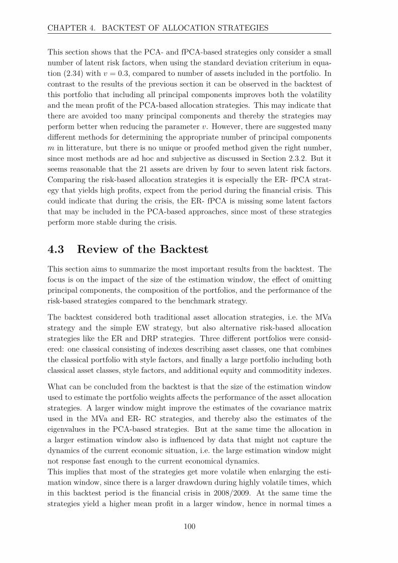
CHAPTER 4. BACKTEST OF ALLOCATION STRATEGIES
This section shows that the PCA- and fPCA-based strategies only consider a smallnumber of latent risk factors, when using the standard deviation criterium in equa-tion (2.34) with v = 0.3, compared to number of assets included in the portfolio. Incontrast to the results of the previous section it can be observed in the backtest ofthis portfolio that including all principal components improves both the volatilityand the mean profit of the PCA-based allocation strategies. This may indicate thatthere are avoided too many principal components and thereby the strategies mayperform better when reducing the parameter v. However, there are suggested manydifferent methods for determining the appropriate number of principal componentsm in litterature, but there is no unique or proofed method given the right number,since most methods are ad hoc and subjective as discussed in Section 2.3.2. But itseems reasonable that the 21 assets are driven by four to seven latent risk factors.Comparing the risk-based allocation strategies it is especially the ER- fPCA strat-egy that yields high profits, expect from the period during the financial crisis. Thiscould indicate that during the crisis, the ER- fPCA is missing some latent factorsthat may be included in the PCA-based approaches, since most of these strategiesperform more stable during the crisis.
4.3 Review of the BacktestThis section aims to summarize the most important results from the backtest. Thefocus is on the impact of the size of the estimation window, the effect of omittingprincipal components, the composition of the portfolios, and the performance of therisk-based strategies compared to the benchmark strategy.
The backtest considered both traditional asset allocation strategies, i.e. the MVastrategy and the simple EW strategy, but also alternative risk-based allocationstrategies like the ER and DRP strategies. Three different portfolios were consid-ered: one classical consisting of indexes describing asset classes, one that combinesthe classical portfolio with style factors, and finally a large portfolio including bothclassical asset classes, style factors, and additional equity and commoditity indexes.
What can be concluded from the backtest is that the size of the estimation windowused to estimate the portfolio weights affects the performance of the asset allocationstrategies. A larger window might improve the estimates of the covariance matrixused in the MVa and ER- RC strategies, and thereby also the estimates of theeigenvalues in the PCA-based strategies. But at the same time the allocation ina larger estimation window also is influenced by data that might not capture thedynamics of the current economic situation, i.e. the large estimation window mightnot response fast enough to the current economical dynamics.This implies that most of the strategies get more volatile when enlarging the esti-mation window, since there is a larger drawdown during highly volatile times, whichin this backtest period is the financial crisis in 2008/2009. At the same time thestrategies yield a higher mean profit in a larger window, hence in normal times a
100
4.3. REVIEW OF THE BACKTEST
larger estimation window implies higher profits, but during highly volatile times oneshould use a shorter window in order to better capture the market dynamics. Theeffect on the Sharpe ratio is dependent on the composition of the portfolio, i.e. theportfolio consisting of the nine assets has an increased Sharpe ratio when using thelarger estimation window, whereas in the other two profits most of the strategieshave a lower Sharpe ratio due to the increased volatility. This shows the positiveeffect of including style factors in a portfolio, which are very low correlated to eachother and thereby the portfolio has good diversification properties which imply morestable profits.
Furthermore, differing sampling periods may yield different degree of smoothing inthe ER- fPCA strategy. The reason that the smoothing parameter λ may differis due to the setup of the performed cross validation as described in Section 3.1.3.Since a smaller sampling period implies that the training- and validation sets getsmaller in the cross validation, which has a large impact on the choice of the pa-rameters. A different degree of smoothing also means that the number of principalcomponents m differs, since the parameter m is determined based on the smootheddata. The more smoothed data is, the less is the number of principal components,since smoothing removes much of the variability of data and thereby the standarddeviations used in equation (2.34) become smaller, hence more principal componentsare avoided. In the considered backtest the same smoothing parameter is selectedfor all setups, whereas the number of basis functions differs. This is an interest-ing observation since the training- and validation sets cover the same time periods,but the portfolios consist of different assets. The selected smoothing parameter isthe highest possible value, which is due large flucations in the included assets ofthe portfolios, in particular the equity and commodity indexes, hence data is moresmoothed as explained in Section 2.1.2.When enlarging the size of the estimation window and the number of assets in-cluded in a portfolio, the ER- fPCA yields higher profits during the backtest, expectfrom the large portfolio, but still has a drawdown during the financial crisis whencompared to other risk-based strategies. This shows that the strategy is better inaccounting for the variability in data during normal times when considering an ap-propriate amount of data, i.e. a large enough estimation window. The reason thatthe strategy not performs that well during the financial crisis in 2008/2009 mightbe explained by a wrong number of principal components, since this parameter isstatic throughout the backtest period, but it can be imagined that the number ofunderlying risk factors increases during a financial crisis. Or data is smoothed toomuch, which can remove valuable variablility. Therefore it should be considered tomake these parameters time-varying.
Excluding principal components that explain little variance in data seems reason-able to do, but the choice of the parameter v that controls the number of principalcomponents is not that straightforward, as discussed in Section 2.3.2, and some ofthe allocation strategies are rather sensitive to this parameter as will be explained
101
CHAPTER 4. BACKTEST OF ALLOCATION STRATEGIES
below.It could be examined in the backtest of the portfolio consisting of nine assets thatomitting components improved the mean profit, but also made the profit morevolatile. In the case of the large portfolio consisting of 21 assets it was more prof-itable to include all principal components than only considering five or six as de-termined by the criterium in equation (2.34). As mentioned above, this could becaused by the large drawdown in the financial crisis due to missing risk factors thatexplain the underlying market movements in this period. For the ER- fPCA strat-egy it can be observed that there is no difference whether to use the number ofprincipal components suggested by the standard deviation criterium or by using asmany components as there are assets in the portfolio.This raises the question of how many principal components that should be included.In order to investigate this, Figure 4.18 shows the Sharpe ratio of the three strategiesthat are based on PCA using a varying number of principal components by tryingdifferent values for the parameter v, i.e. considering v = 0.1, 0.2, . . . , 0.9. The reasonto consider the Sharpe ratio is to find out which number of principal componentsthat makes the PCA-based strategies most profitable. The results for the portfolioconsisting of nine and 21 assets can be seen in the left and right panel of Figure4.18, respectively.It can be observed that the three strategies behave very different when changing thenumber of principal components. The Sharpe ratio of the ER- PCA strategy doesnot change that much, but decreases a bit when omitting some components. This iscaused by the fact that the profit volatility increases while the mean profit decreasesin proportion to each other. The ER- PCA RC strategy might yield a higher Sharperatio when only including a small number of components, whereas the DRP strategyin the case of the nine assets performs worse by omitting components, but in thecase of 21 assets yields the highest Sharpe ratio when considering 11 components.In both strategies the profit gets more volatile and at the same time the mean profitincreases, but to different degree.Studying different methods and thresholds for how many principal components thatshould be included may improve the performance of the PCA-based strategies, butis beyond the scope of this thesis.
102
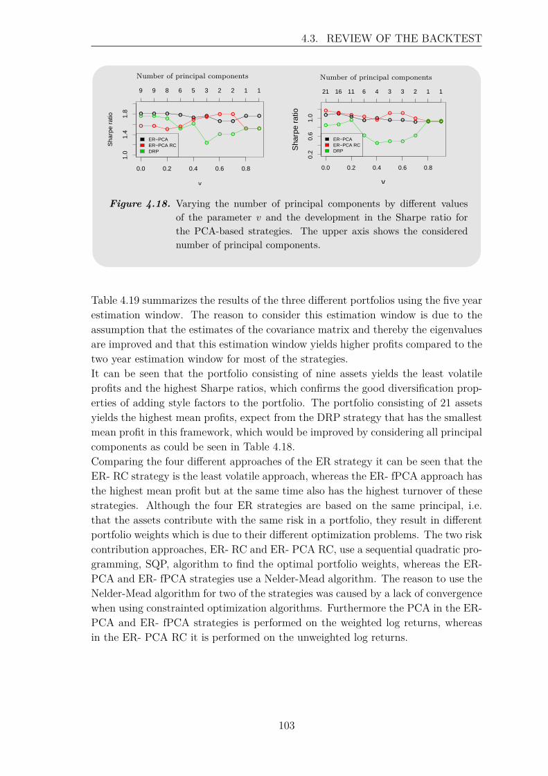
4.3. REVIEW OF THE BACKTEST
Number of principal components
0.0 0.2 0.4 0.6 0.8
1.0
1.4
1.8
v
Sha
rpe
ratio
9 9 8 6 5 3 2 2 1 1
ER−PCAER−PCA RCDRP
Number of principal components
0.0 0.2 0.4 0.6 0.8
0.2
0.6
1.0
v
Sha
rpe
ratio
21 16 11 6 4 3 3 2 1 1
ER−PCAER−PCA RCDRP
Figure 4.18. Varying the number of principal components by different valuesof the parameter v and the development in the Sharpe ratio forthe PCA-based strategies. The upper axis shows the considerednumber of principal components.
Table 4.19 summarizes the results of the three different portfolios using the five yearestimation window. The reason to consider this estimation window is due to theassumption that the estimates of the covariance matrix and thereby the eigenvaluesare improved and that this estimation window yields higher profits compared to thetwo year estimation window for most of the strategies.It can be seen that the portfolio consisting of nine assets yields the least volatileprofits and the highest Sharpe ratios, which confirms the good diversification prop-erties of adding style factors to the portfolio. The portfolio consisting of 21 assetsyields the highest mean profits, expect from the DRP strategy that has the smallestmean profit in this framework, which would be improved by considering all principalcomponents as could be seen in Table 4.18.Comparing the four different approaches of the ER strategy it can be seen that theER- RC strategy is the least volatile approach, whereas the ER- fPCA approach hasthe highest mean profit but at the same time also has the highest turnover of thesestrategies. Although the four ER strategies are based on the same principal, i.e.that the assets contribute with the same risk in a portfolio, they result in differentportfolio weights which is due to their different optimization problems. The two riskcontribution approaches, ER- RC and ER- PCA RC, use a sequential quadratic pro-gramming, SQP, algorithm to find the optimal portfolio weights, whereas the ER-PCA and ER- fPCA strategies use a Nelder-Mead algorithm. The reason to use theNelder-Mead algorithm for two of the strategies was caused by a lack of convergencewhen using constrainted optimization algorithms. Furthermore the PCA in the ER-PCA and ER- fPCA strategies is performed on the weighted log returns, whereasin the ER- PCA RC it is performed on the unweighted log returns.
103
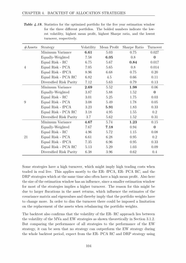
CHAPTER 4. BACKTEST OF ALLOCATION STRATEGIES
Table 4.19. Statistics for the optimized portfolio for the five year estimation windowfor the three different portfolios. The bolded numbers indicate the low-est volatility, highest mean profit, highest Sharpe ratio, and the lowestturnover, respectively.
#Assets Strategy Volatility Mean Profit Sharpe Ratio TurnoverMinimum Variance 6.61 5.03 0.75 0.027Equally-Weighted 7.58 6.05 0.8 0Equal Risk - RC 6.75 5.67 0.84 0.017
4 Equal Risk - PCA 7.05 5.65 0.8 0.014Equal Risk - fPCA 8.96 6.68 0.75 0.20Equal Risk - PCA RC 6.82 4.5 0.66 0.11Diversified Risk Parity 7.12 5.63 0.79 0.13Minimum Variance 2.69 5.52 1.98 0.06Equally-Weighted 3.87 5.88 1.52 0Equal Risk - RC 3.01 5.25 1.75 0.03
9 Equal Risk - PCA 3.08 5.49 1.78 0.05Equal Risk - fPCA 3.23 5.91 1.83 0.33Equal Risk - PCA RC 3.18 4.95 1.55 0.2Diversified Risk Parity 3.7 5.62 1.52 0.31Minimum Variance 4.67 5.74 1.23 0.15Equally-Weighted 7.67 7.18 0.94 0Equal Risk - RC 4.96 5.72 1.15 0.08
21 Equal Risk - PCA 6.61 6.28 0.95 0.2Equal Risk - fPCA 7.35 6.96 0.95 0.33Equal Risk - PCA RC 5.13 5.29 1.03 0.09Diversified Risk Parity 6.38 3.96 0.62 0.4
Some strategies have a high turnover, which might imply high trading costs whentraded in real live. This applies mostly to the ER- fPCA, ER- PCA RC, and theDRP strategies which at the same time also often have a high mean profit. Also herethe size of the estimation window has an influence, since a smaller estimation windowfor most of the strategies implies a higher turnover. The reason for this might bedue to larger flucations in the asset returns, which influence the estimates of thecovariance matrix and eigenvalues and thereby imply that the portfolio weights haveto change more. In order to dim the turnover there could be imposed a limitationon the replacement of the assets when rebalancing the portfolio weights.
The backtest also confirms that the volatility of the ER- RC approach lies betweenthe volatility of the MVa and EW strategies as shown theoretically in Section 3.1.2.But comparing the performance of all strategies to the performance of the EWstrategy, it can be seen that no strategy can outperform the EW strategy duringthe whole backtest period, expect from the ER- PCA RC and DRP strategy using
104
4.3. REVIEW OF THE BACKTEST
the portfolio consisting of four classical assets and using a two year sampling periodas can be seen in Figure 4.5.The good performance of the simple benchmark strategy rises the question whetherthe work of implementing the rather complicated risk-based strategies can pay off?This is difficult to answer, but a great disadvantage of the EW strategy is thatit is not possible to control the risk of this strategy. The ER strategies are agood tradeoff between the EW strategy that has a lack of risk monitoring and theMVa strategy that only focuses on risk. Moreover the MVa strategy is not thatdiversified as measured by the Herfindahl index, which applies in all frameworksand all portfolios, since it gives much weight to low volatile assets.It should also be noted that during the whole backtest period there has been fallinginterest rates, which has a positive effect on the returns of bonds. Since bondsare very low volatile the MVa strategy allocates mostly in bonds, i.e. the MVastrategy benefits from the falling interest rates in the backtest period. This shouldbe considered when comparing the different strategies with the MVa strategy, sinceit is not ensured that the MVa strategy always will perform as good as it does inthis selected backtest period.
Besides the performance measured by the profit, turnover, and diversification, of thedifferent asset allocation strategies it is also important to consider the computationaleffort needed to find the portfolio weights. The computations for estimating thecovariance matrix and the eigenvalues in the PCA-based strategies are fairly fast.On other hand, the fPCA-based strategy has to determine additional parameters, i.e.the number of basis functions K and the smoothing parameter λ, which is done byusing cross validation. Afterwards data has to be smoothed using these parameters,and then the fPCA can be performed to estimate the eigenvalues needed to find theoptimal portfolio weights. This implies that this strategy is more complex and timeconsuming than the other strategies.
The performance of the risk-based strategies might be significantly improved whenestimations errors in the covariance matrix and the eigenvalues are ensured to beminimal. The constraint of long-only portfolio might also have an impact on theperformance of the strategies. This is investigated by [Kind, 2013] who reports thatallowing long-short portfolios improves the diversification properties of the risk-based allocation strategies, but it does not improve the performance the strategies.It should of course be noted that good diversification of a portfolio does not neces-sarily imply good performance.In the backtest it should be considered to include other performance measures be-sides the volatility of the profit, mean profit, Sharpe ratio, turnover, and Herfindahlindex. As can be seen from the above discussion, often more volatile profit can beexplained by a large drop in the cumulative return, this could be measured by thedrawdown or maximum drawdown.
105

Recapitulation 5The main conclusion of this thesis is that most of the introduced risk-based assetallocation strategies outperform the Equally-Weighted strategy for medium-sizedportfolios during times of high volatility. I expect the outperformance to be evenmore significant for larger portfolios, especially for the functional approach of theEqual Risk strategy. Furthermore, I conclude that these strategies perform verystable, which is especially preferable for long-term investors.
The purpose of this thesis has been to establish asset allocation strategies that arebased on latent risk factors instead of traditional allocation strategies that allo-cate by asset classes. The reason to consider latent risk factors is due to the factthat assets consist of latent factors and therefore there should be diversificationbenefits when allocating in these factors. The motivation to consider alternative,risk-based strategies is among others due to the recent financial crisis in 2008/2009which showed that many traditional asset allocation strategies that are based on theestimates of mean and variance could not capture the heavy left tail of the returndistribution and thereby did not perform well. Therefore it is interesting to considerrisk-based strategies, since these strategies allocate by considering the underlyingrisk factors, hence these strategies might have captured the risks assets where ex-posed to during the crisis. I have placed much emphasis on projection methodsto extract the underlying risk factors, namely principal component analysis and itsfunctional variant, functional principal component analysis.
Principal component analysis is a statistical method to transform the original vari-able space into a lower dimensional space without losing too much information.The reason to consider a lower dimensional representation of the original variablespace is due to the purpose of only considering the important features in data. Theaim is to reduce the asset space consisting of assets returns to latent factors, whichare represented by the principal components. The principal components are lin-ear combinations of the original asset returns and are constructed such that thefirst component is variance maximizing and the subsequent components are vari-ance maximizing with the constraint of being orthogonal to the preceding compo-nents. Functional principal component analysis is based on the same principles,but considers data to have an underlying functional form that can be modelled by
107
CHAPTER 5. RECAPITULATION
univariate functions. The functional approach accounts for the dependence of theunderlying observations over time and thereby models the asset returns’ underlyingfunctional process. This implies that the functional data analysis can handle assetswith different sampling rates or missing observations, which is a great advantage tomultivariate analysis. Thereby eigenfunctions can be modelled over time, which iscontrast to principal component analysis, that gives a static, non-temporal estimateof the eigenvectors. Hence it is assumed that the functional framework is betterin caputuring the variability in asset returns over time. In order to use functionalprincipal component analysis, data has to be transformed to functional data. Thetransformation is done using basis functions, which are the counterpart to basis vec-tors in functional space. Since asset returns are non-periodic, I introduced B-splinesas basis functions. Furthermore a technique for smoothing data has been describedwhich uses a roughness penalty and is based on weighted least squares. After study-ing these methods to extract risk factors, some risk-based asset allocation strategieshave been introduced.
The main focus of this thesis was on the Equal Risk strategy which covers overdifferent techniques. One way to consider this strategy is by choosing the portfolioweights of the single assets in a portfolio such that every asset contributes with thesame risk to the portfolio. This approach can either be considered in the originalasset space or it can be transformed into the principal space by using principalcomponent analysis. Another way to consider this approach is to select the portfolioweights of the single assets in a portfolio such that a principal component analysisperformed on the asset returns yields as equal as possible volatility in the principalcomponent directions. This approach was also performed using functional principalcomponent analysis. Note that the Equal Risk strategy can be considered as atradeoff of the Minimum Variance and Equally-Weighted strategies in terms of theportfolio variance, i.e. the risk associated when using this strategy.
For the purpose of investigating the performance of the different asset allocationstrategies I considered a backtest on historical data. A walk-forward backtest withrolling estimation window was used to compute the portfolio weights every month,where different sizes of the estimation window were analyzed. Using the assumptionthat short-selling is not allowed, three different portfolios were backtested. Theseportfolios included a different number of assets and different types of assets in orderto investigate the behaviour of the different strategies. Moreover, I focused oninvestigating the impact of omitting some principal components, i.e. to reduce thenumber of underlying risk factors. Selecting a method and a threshold for decidingon how many principal components that should be omitted is a difficult choice andI found ambivalent results regarding this issue. In some cases the mean profit ofa risk-based strategy that uses principal component analysis could be improved byomitting components with the cost of a higher volatility of the profit, which in allcases led to a reduced Sharpe ratio compared with the performance of the strategiesthat used all principal components. Further research on this topic could improve
108
the performance of the risk-based strategies that are based on principal componentanalysis.
From the backtest it could also be concluded that the different risk-based strategiesperform different when varying the size of the estimation window and the composi-tion of the portfolio. During normal times a larger estimation benefits the risk-basedstrategies, but during highly volatile periods a shorter estimation window should beused in order to capture the exposure to the risk factors present during this pe-riod. The risk-based strategies most of the time had a lower volatile profit than theEqually-Weighted strategy, the benchmark strategy. At the same time the bench-mark strategy often had a higher mean profit than the risk-based strategies.
There is still room for improvement of the risk-based strategies. There may beplaced more emphasis on the estimation of the covariance matrix, since small esti-mation errors can cause large deviations in the computation of the risk contributionsor in the principal component analysis and thereby in the selected portfolio weights.Furthermore, the process of smoothing data in the functional approach may be in-vestigated more comprehensively since this also can cause a completely differentallocation. In the setup of the backtest it should be considered to make the parame-ters time-varying, i.e. to compute the number of principal components, the numberof basis functions, and the smoothing parameter for every estimation. This mightimprove the principal component analysis-based strategies, since it seems reasonablethat the number of underlying risk factors varies over time, and that data has tobe smoothed to different degree over time in the functional approach of the EqualRisk strategy. This has been disgraded in this thesis due to lack of time and therebysimplification of the implementation of the backtest. It could also be considered toimplement the other principal component analysis-based strategies using the func-tional approach, since there only is transformed one Equal Risk approach to makeuse of functional principal component analysis. Furthermore, in the setup of thebacktest there still are disregarded observations for assets with different samplingrates in the functional approach for ease of the implementation of the backtest,although it theoretically is possible to include all observations. Hence includingall available observations of all assets might improve the functional approch. Thisthesis focuses on the standard deviation as the measure of risk, but it could beinvestigated if other measures of risk, e.g. the quantile-based value at risk, VaR,or shortfall-based measures, could be used in the computation of the risk contribu-tions in the Equal Risk strategy. Furthermore, other projections methods could beconsidered, e.g. independent component analysis.
The usage of risk-based asset allocation strategies is not that widespread yet, butseveral Nordic investors allocate a part of there assets in alternative, risk-basedstrategies. To mention some of them: the Danish pension fund PKA, the Swedishpension fund SPK, and the Swedish state pension funds AP2 and AP3. The Danishpension fund PKA changed their equity strategy to also allocate in alternative, risk-based strategies in 2012. [Liinanki, February/March 2015] Also the government
109

CHAPTER 5. RECAPITULATION
pension fund of Norway, SPU, also called ’The Oil Fund’ is known to use factorinvesting. It is one of the world largest pension funds, which at the end of 2012managed $685 billion. [Ang, 2014] The reason that many investor still are hesitatingto use risk-based allocation strategies is that it can be time consuming to understandand implement these allocation strategies. [Liinanki, February/March 2015]
110
Bibliography
A. Meucci, A. Santangelo, R. Deguest. Measuring Portfolio Diversifcation Basedon Optimized Uncorrelated Factors. 2014.
A. Alexanderian. A Brief Note on the Karhunen-Loeve Expansion, 2013.
A. Ang. Asset Management: A Systematic Approach to Factor Investing. OxfordUniversity Press, 2014.
T. Björk. Arbitrage Theory in Continuous Time. Oxford University Press, 2009.
R. Cangelosi and A. Goriely. Component Retention in Principal ComponentAnalysis with Application to cDNA Microarray Data. Biology Direct, 2007.
M. A. Crain. A Literature Review of the Size Effect. 2011.
P. Craven and G. Wahba. Smoothing Noisy Data with Spline Functions.Numerische Mathematik, 31:377 – 403, 1979.
M. Guan. Principal Component Analysis in Portfolio Management, 2013. URLhttps://systematicedge.wordpress.com/2013/06/02/
principal-component-analysis-in-portfolio-management/.
H. Lohre, H. Opfer, G. Orszag. Diversifying Risk Parity. JEL Classification, 2013.
R. J. Hyndman. Fast Computation of Cross-validation in Linear Models, 2014.URL http://robjhyndman.com/hyndsight/loocv-linear-models/.
J. Friedman, T. Hastie, R. Tibshirani. The Elements of Statistical Learning.Springer-Verlag New York, 2009.
J. O. Ramsay , B. W. Silverman. Functional Data Analysis. SpringerScience+Business Media, Inc., 2005.
J. O. Ramsay, G. Hooker, S. Gaves. Functional Data Analysis with R andMATLAB. Springer Science+Business Media, 2009.
J. O. Reilly, S. O. Barba, N. Pavlov. Growth vs. Value Trading Strategies, 2003.URL https://faculty.fuqua.duke.edu/~charvey/Teaching/
BA453_2003/CPAM/HTML/Index.htm.
111
BIBLIOGRAPHY
J. Peng and D. Paul. A Geometric Approach to Maximum Likelihood Estimationof the Functional Principal Components From Sparse Longitudinal Data.Journal of Computational and Graphical Statistics, 2012.
J. Y. Campbell, A. W. Lo, A. C. MacKinlay. The Econometrics of FinancialMarkets. Princeton University Press, 1997.
K. V. Mardia, J.T. Kent, J. M. Bibby. Multivariate Analysis. Academic Press,1994.
C. Kind. Risk-Based Allocation of Principal Portfolios. 2013.
A. Lesniewski. Interest Rates and FX Models - 3. Girsanov, Numeraires, and AllThat. 2008.
C. Liinanki. Lessons and Experiences from the Nordic Pioneers. Nordic FundSelection Journal, February/March 2015.
F. Longin. The Choice of the Distribution of Asset Returns: How Extreme ValueTheory can Help? Journal of Banking and Finance, 29:1017–1035, 2005.
D. G. Luenberger. Investment Science. Oxford University Press, 2009.
M. Grinblatt and S. Titman. Financial Market and Corporate Strategy.McGraw-Hill Higher Education, 2002.
S. Mesomeris. Risk Premia in Asset Allocation, 2013. URLhttps://secure.cfauk.org/assets/2891/Spyros_Mesomeris___
A_new_asset_allocation_paradigm.pdf.
A. Meucci. Managing Diversification. Bloomberg Education & QuantitativeResearch and Education Paper, 2010.
L. J. Overby. CAPM, Factor Models and APT, 2010. URLhttp://www.juloverby.dk/courses/cfi/slides/mean_var_3.pdf.
S. Maillard, T. Roncalli, J. Teiletche. On the Porperties of Equally-weighted RiskContributions Portfolios. 2009.
G. A. F. Seber. Multivariate Observations. WILEY, 2004.
SP Dow Jones Indices. SP 500, 2015. URLhttp://us.spindices.com/indices/equity/sp-500.
D. Stefanovits. Equal Contributions to Risk and Portfolio Construction. MasterThesis, ETH Zurich, 2010.
T. E. Copeland and J. F. Weston. Financial Theory and Corporate Policy.Addison-Wesley Publishing Company, 1988.
112

BIBLIOGRAPHY
D. Tasche. Capital Allocation to Business Units and Sub-Portfolios: the EulerPrincipal. 2008.
T. Tvedebrink. Slides from MAT8 Data Mining Course, 2014.
J.-T. Zhang. Analysis of Variance for Functional Data. CRC Press, 2014.
E. Zivot. Introduction to Computational Finance and Financial Econometrics -Return Calculations, 2015. URL http://faculty.washington.edu/
ezivot/econ424/returncalculationslides.pdf.
113

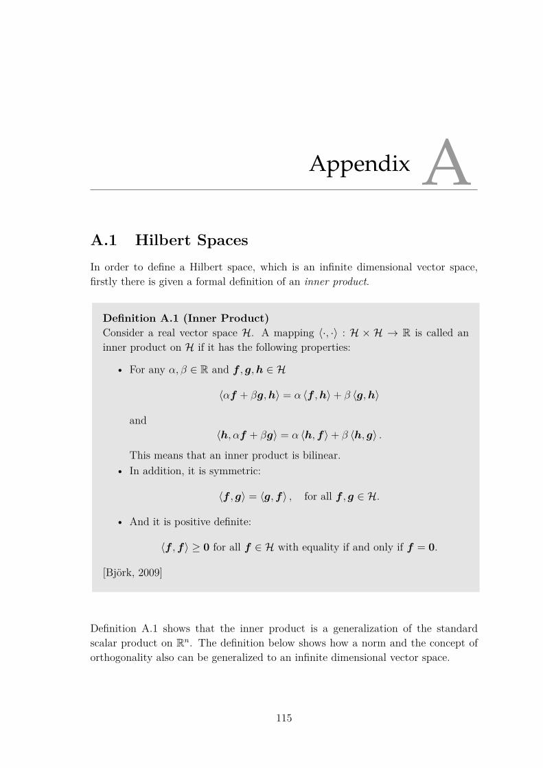
Appendix AA.1 Hilbert SpacesIn order to define a Hilbert space, which is an infinite dimensional vector space,firstly there is given a formal definition of an inner product.
Definition A.1 (Inner Product)Consider a real vector space H. A mapping 〈·, ·〉 : H × H → R is called aninner product on H if it has the following properties:
• For any α, β ∈ R and f , g,h ∈ H
〈αf + βg,h〉 = α 〈f ,h〉+ β 〈g,h〉
and〈h, αf + βg〉 = α 〈h,f〉+ β 〈h, g〉 .
This means that an inner product is bilinear.• In addition, it is symmetric:
〈f , g〉 = 〈g,f〉 , for all f , g ∈ H.
• And it is positive definite:
〈f ,f〉 ≥ 0 for all f ∈ H with equality if and only if f = 0.
[Björk, 2009]
Definition A.1 shows that the inner product is a generalization of the standardscalar product on Rn. The definition below shows how a norm and the concept oforthogonality also can be generalized to an infinite dimensional vector space.
115
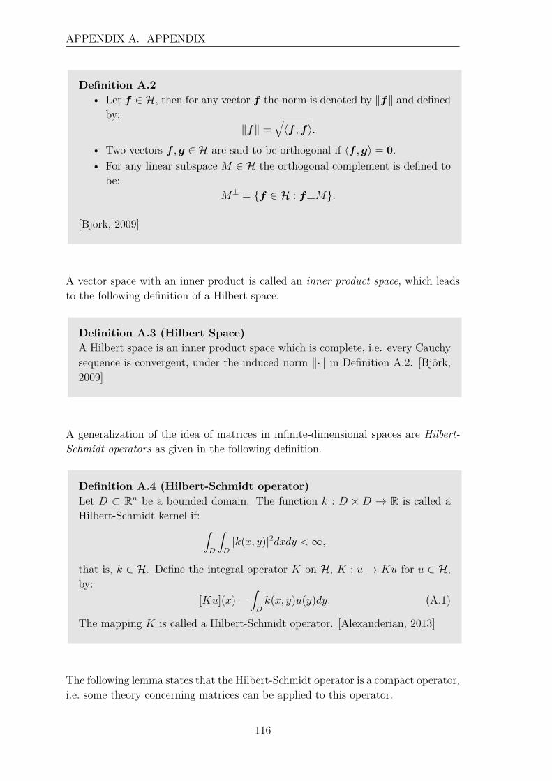
APPENDIX A. APPENDIX
Definition A.2• Let f ∈ H, then for any vector f the norm is denoted by ‖f‖ and defined
by:‖f‖ =
√〈f ,f〉.
• Two vectors f , g ∈ H are said to be orthogonal if 〈f , g〉 = 0.• For any linear subspace M ∈ H the orthogonal complement is defined to
be:M⊥ = f ∈ H : f⊥M.
[Björk, 2009]
A vector space with an inner product is called an inner product space, which leadsto the following definition of a Hilbert space.
Definition A.3 (Hilbert Space)A Hilbert space is an inner product space which is complete, i.e. every Cauchysequence is convergent, under the induced norm ‖·‖ in Definition A.2. [Björk,2009]
A generalization of the idea of matrices in infinite-dimensional spaces are Hilbert-Schmidt operators as given in the following definition.
Definition A.4 (Hilbert-Schmidt operator)Let D ⊂ Rn be a bounded domain. The function k : D × D → R is called aHilbert-Schmidt kernel if: ∫
D
∫D|k(x, y)|2dxdy <∞,
that is, k ∈ H. Define the integral operator K on H, K : u → Ku for u ∈ H,by:
[Ku](x) =∫Dk(x, y)u(y)dy. (A.1)
The mapping K is called a Hilbert-Schmidt operator. [Alexanderian, 2013]
The following lemma states that the Hilbert-Schmidt operator is a compact operator,i.e. some theory concerning matrices can be applied to this operator.
116
A.1. HILBERT SPACES
Lemma A.5Let D be a bounded domain in Rn and let k be a Hilbert-Schmidt kernel.Then the integral operator K : H → H given by equation (A.1) is a compactoperator. [Alexanderian, 2013]
Proof. Omitted.
The following theorem generalizes the result that any positive semi-definite matrixis the Gram matrix of a set of vectors to Hilbert spaces.
Theorem A.6 (Mercer’s Theorem)Suppose that k(s, t) is a symmetric, continuous, and nonnegative definite kernelfunction on D × D. Suppose further that the corresponding Hilbert-Schmidtoperator K is positive. Then there exists an orthonormal set of eigenfunctionsξj(x) and eigenvalues λj such that:
k(s, t) =∞∑j=1
λjξj(s)ξj(t),
where convergence is absolute and uniform on D ×D. [Alexanderian, 2013]
Proof. Omitted.
Compact self-adjoint operators on infinite dimensional Hilbert spaces act very sim-iliar to symmetric matrices.
Theorem A.7 (Spectral Theorem)LetH be a Hilbert space and let T : H → H be a compact self-adjoint operator.Then, H has an orthonormal basis ξi of eigenvectors of T corresponding toeigenvalues λi. [Alexanderian, 2013]
Proof. Omitted.
117
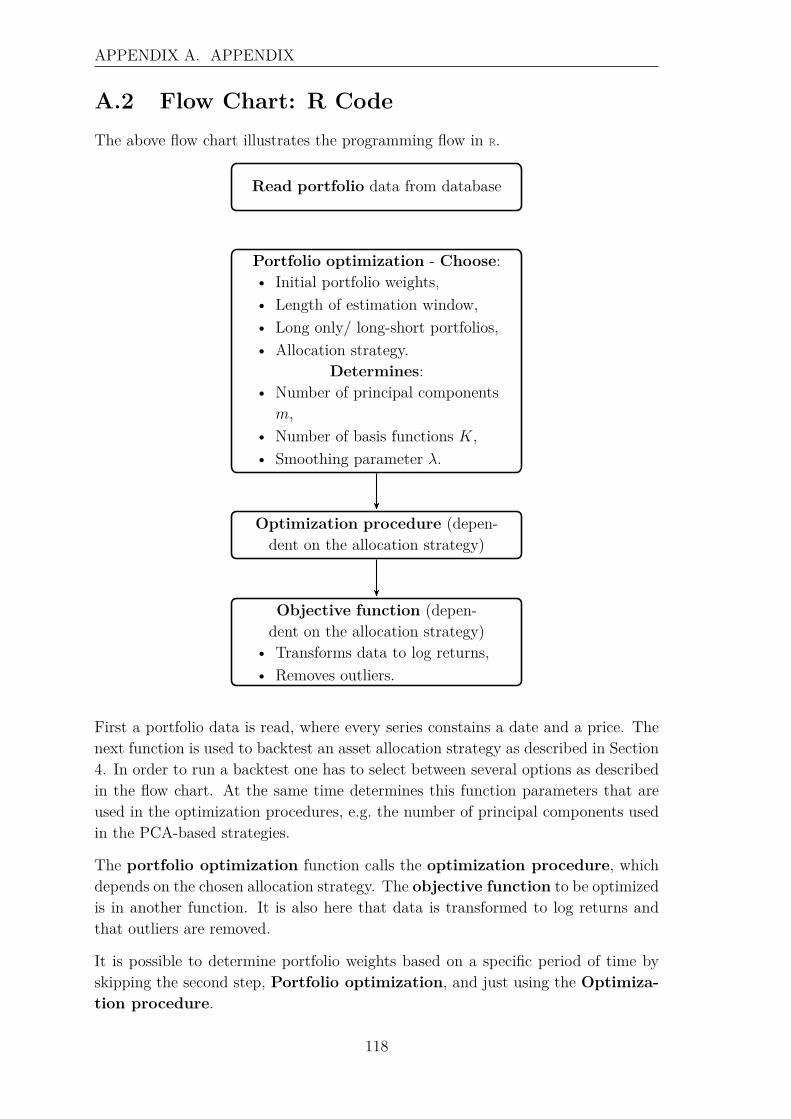
APPENDIX A. APPENDIX
A.2 Flow Chart: R CodeThe above flow chart illustrates the programming flow in R.
Read portfolio data from database
Portfolio optimization - Choose:• Initial portfolio weights,• Length of estimation window,• Long only/ long-short portfolios,• Allocation strategy.
Determines:• Number of principal componentsm,
• Number of basis functions K,• Smoothing parameter λ.
Optimization procedure (depen-dent on the allocation strategy)
Objective function (depen-dent on the allocation strategy)
• Transforms data to log returns,• Removes outliers.
First a portfolio data is read, where every series constains a date and a price. Thenext function is used to backtest an asset allocation strategy as described in Section4. In order to run a backtest one has to select between several options as describedin the flow chart. At the same time determines this function parameters that areused in the optimization procedures, e.g. the number of principal components usedin the PCA-based strategies.
The portfolio optimization function calls the optimization procedure, whichdepends on the chosen allocation strategy. The objective function to be optimizedis in another function. It is also here that data is transformed to log returns andthat outliers are removed.
It is possible to determine portfolio weights based on a specific period of time byskipping the second step, Portfolio optimization, and just using the Optimiza-tion procedure.
118