Statistical method for prediction of gait kinematicswith Gaussian process regression

Youngmok Yun a, Hyun-Chul Kim b, Sung Yul Shin b, Junwon Lee b, Ashish D. Deshpande a,Changhwan Kim b,n

a Department of Mechanical Engineering, The University of Texas at Austin, Austin, TX, USAb The Center of Bionics, Korea Institute of Science and Technology, Seoul, South Korea

a r t i c l e i n f o

Article history:Accepted 17 September 2013

Keywords:Gait patternStatisticsGaussian process regressionStochastic analysis

a b s t r a c t

We propose a novel methodology for predicting human gait pattern kinematics based on a statistical andstochastic approach using a method called Gaussian process regression (GPR). We selected 14 bodyparameters that significantly affect the gait pattern and 14 joint motions that represent gait kinematics.The body parameter and gait kinematics data were recorded from 113 subjects by anthropometricmeasurements and a motion capture system. We generated a regression model with GPR for gait patternprediction and built a stochastic function mapping from body parameters to gait kinematics based on thedatabase and GPR, and validated the model with a cross validation method. The function can not onlyproduce trajectories for the joint motions associated with gait kinematics, but can also estimate theassociated uncertainties. Our approach results in a novel, low-cost and subject-specific method forpredicting gait kinematics with only the subject's body parameters as the necessary input, and alsoenables a comprehensive understanding of the correlation and uncertainty between body parametersand gait kinematics.

& 2013 Elsevier Ltd. All rights reserved.

1. Introduction

Many recent attempts to understand and predict human gaitpattern utilize model-based optimization techniques. Thisapproach hypothesizes mathematical models and cost functionsof the moving bodies, and determines the optimized motion ofmodel. Typical examples of the cost function include total meta-bolic energy (Anderson and Pandy, 2001) and total muscle effort(Xiang et al., 2011), and the models range from simple link models(Srinivasan and Ruina, 2006; Geyer et al., 2005) to elaboratebiomechanical models involving muscles, tendons, varyingmoment arms and body segments (Anderson and Pandy, 2001;Delp et al., 2007).

While the model-based optimization methods have led toadvances in fields such as biomechanics of walking, lower-limbrehabilitation, and biped machine walking (Neptune et al., 2009;Zajac et al., 2003; Bessonnet et al., 2004), there are significantlimitations to this approach. The optimization methods needmechanical and biomechanical models for describing the humanmotion. Assumptions and simplifications are inherent, even in themost advanced models, resulting in limitations of the methods.

The choice of cost function affects the results significantly and it isa topic of ongoing scientific debate (Todorov, 2004). Althoughreasonable choices have been made, it is difficult to capture thecomplexities of human walking with one specific cost function.Most optimization methods output a deterministic pattern. How-ever, the human movements possess inherent variability andchange with time, gender, age, body features and also the emo-tional state (Blanc et al., 1999; Kerrigan et al., 1998; Cunninghamet al., 1982; Escalante et al., 2001; Murray et al., 1964; Samsonet al., 2001; Macellari et al., 1999). Moreover, evidence shows thatwalking may involve randomness (Hausdorff et al., 1995), which isimpossible to capture with the deterministic optimization meth-ods, even in a hypothetical case of fully modeled system.

Statistics-based methods provide an alternative approach forgait pattern prediction because these methods are free of anypredetermined biomechanical models and cost functions, and caninherently handle the deviations and uncertainty in human walk-ing. Although statistical methods have been employed to investi-gate the effects of body parameters on the gait pattern, e.g. gender(Blanc et al., 1999; Kerrigan et al., 1998) and age (Cunninghamet al., 1982; Escalante et al., 2001), typically, only the effect of asingle factor is analyzed and no functional mapping is developed.Over the last two decades, the introduction of motion capturedevices in gait pattern research has led to the collection of a largeamount of data (Kadaba et al., 1990; Davis et al., 1991). And the

Contents lists available at ScienceDirect

journal homepage: www.elsevier.com/locate/jbiomechwww.JBiomech.com

Journal of Biomechanics

0021-9290/$ - see front matter & 2013 Elsevier Ltd. All rights reserved.http://dx.doi.org/10.1016/j.jbiomech.2013.09.032

n Corresponding author.E-mail addresses: yunyoungmok@utexas.edu (Y. Yun), ckim@kist.re.kr (C. Kim).

Journal of Biomechanics 47 (2014) 186–192

recently developed machine learning algorithms such as neuralnetwork (Bishop, 1995), support vector machine (Smola andSchölkopf, 2004), and Gaussian process regression (Rasmussen,2006) provide novel and computationally powerful statistical toolsfor processing such a large-scale data.

Our goal is to develop a statistical and stochastic approach forgait kinematics prediction using a large-scale database. We pre-sent a method that builds a stochastic function mapping whoseinput is body parameters and output is the gait pattern kinematics.The developed function mapping is a numerical model, sometimesreferred to as a black-box model, and it is created through theGaussian process regression (GPR) algorithm (Rasmussen, 2006).By incorporating the variability in the database in the modelingformulation, GPR can produce a stochastic function whose outputis a probability distribution of the predicted gait kinematics ratherthan a strictly deterministic value.

In addition, we provide a Matlab/Octave toolbox, ‘Gait Kine-matics Prediction Toolbox’ and a database ‘KIST Human GaitPattern Data’ for gait kinematics prediction along with a moredetailed description of the presented method, as SupplementalMaterial.

2. Methods

2.1. Data collection with human subjects

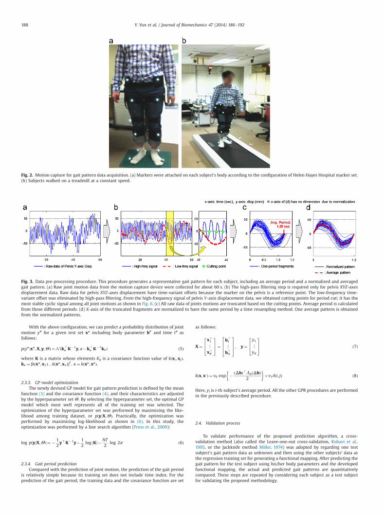
A total of 113 healthy subjects (50 males and 63 females) participated in thestudy. Ethics rules of the Institutional Review Board (IRB) of Korea Institute ofScience and Technology (KIST) were followed during data acquisition (IRB Approvalnumber: 2012-006). We chose the subjects so as to maintain a uniform distributionin age between years 20 and 69. For each subject, age and gender were recorded,and 12 body parameters (Fig. 1) were measured using the method described byChandler et al. (1975). Gait kinematic data were acquired with a motion capturesystem (Motion Analysis Inc.) with eight cameras, and the Helen Hayes Hospitalmarker set (15 markers on the lower-body, Kadaba et al., 1990) was adopted.Because we were collecting data with a large number of participants, we decided toattach markers on the subject's clothing rather than on the skin or on a bodysuit.We fixed a velcro belt tightly on the subject's clothed body and then attachedmarkers on the velcro belt (Fig. 2(a)). During the experiment, subjects were askedto walk at a constant speed, 3 km/h, which is a normal walking speed (Ryu et al.,2006) on a treadmill (Fig. 2(b)). When a stable walking speed was reached, motioncapture data were recorded for 1 min (approximately 40–60 walking cycles).

The 3-D XYZ marker position data were converted into human joint space(Kadaba et al., 1990). A marker attached on the pelvis was used as a referencepoint, and all other relative joint motions were calculated. A total of 14 jointdisplacements and rotations were calculated from 3-D position data including:pelvis X=Y=Z-axis displacement, pelvis rotation, right/left hip adduction/flexion/rotation, right/left knee flexion, and right/left ankle flexion. These 14 kinematicmeasures are the gait pattern outputs and other minor joint rotations (e.g. kneevarus) were not considered in this method.

2.2. Data pre-processing

Raw data from the motion capture device contain 14 joint motions whose timelength is about 60 s, including 40–60 gait cycles (Fig. 3(a)). First, for pelvis XYZ-axesdisplacement, the low-frequency offset of the raw data is eliminated by high passfiltering; because the marker on pelvis is used as a reference point, time-variantoffset exists. Since the filtered pelvis Y -axis displacement data have the most stablecyclic pattern among all motions (Fig. 3), we used it to determine the cutting pointsdenoting the start and end of one walking cycle (Fig. 3(a)). Second, all raw data ofjoint motions are divided into several one-period fragments based on the cuttingpoints. This cut in the period was automatically performed by a computer programin Matlab (Mathworks Inc.). The average period is calculated from those differentperiods (Fig. 3(c)). Third, because the truncated one-period joint motion fragmentshave varying periods, all one-period joint motions were normalized to have thesame period by a time resampling method. Then one average pattern is obtainedfrom the normalized patterns (Fig. 3(d)). The averaged and normalized gait pattern,and averaged period represent one subject's gait pattern. All of the regressionprocedures are conducted with these normalized gait patterns and averagedperiods. The final result of regression is also a normalized gait pattern and aperiod. Then the normalized gait pattern is stretched back with the predictedperiod by time resampling.

2.3. Gaussian process regression algorithm for gait pattern prediction

Gait pattern prediction is regarded as a nonlinear regression task and weimplemented the Gaussian process regression (GPR) algorithm (Rasmussen, 2006)for generating a functional mapping between the input variables (14 bodyparameters) and output gait pattern (14 joint motions for gait kinematics and gaitperiod). First, we describe the GPR algorithm to predict joint motions from Sections2.3.1 and 2.3.3, and then explain the algorithm to predict gait period in Section2.3.4.

2.3.1. Definition of training setFor the prediction of normalized joint motions, the training input vector x, the

training output scalar y, and their sets X and y are defined as follows:

X¼x>1

⋮x>N�T

264

375¼

b>1 t1⋮ ⋮b>1 tT

b>2 t1⋮ ⋮b>N tT

26666666664

37777777775; y¼

y1⋮

yN�T

264

375 ð1Þ

where b is a vector denoting the subject's body parameter, N is the total number ofsubjects, t denotes a time index in the normalized time frame, T is the last index ofthe normalized time frame, and y is a gait pattern value (given as a distance or anangle) corresponding to its x. For example, if a training set is made for ankle flexionpattern, xði�1Þ�Tþ j includes the body parameter bi of i-th subject and the j-th timeindex tj, and corresponding y is ankle flexion angle for the given condition. Thistraining set is built for all of the 14 joint motions that represent gait kinematics.

2.3.2. Design of Gaussian process modelA Gaussian process is completely defined by its mean function and covariance

function (Rasmussen, 2006), as follows:

f ðxÞ � GPðmðxÞ; kðx; x′ÞÞ ð2Þwhere mean function mðxÞ ¼ E½f ðxÞ�, and covariance function kðx;x′Þ ¼ E½ðf ðxÞ�mðxÞÞðf ðx′Þ�mðx′ÞÞ�.

In our GP model, the mean function and the covariance function are deter-mined as follows:

mðxÞ ¼ 0 ð3Þ

kðx; x′Þ ¼ ν0 exp � ðΔbÞ>ΛbðΔbÞþλtΔt2

2

� �þν1δði; jÞ ð4Þ

whereΔb is defined as b�b′ and Δt is defined as t�t′. δði; jÞ is the Kronecker delta

function. Λb is a diagonal matrix whose elements are λb1…λb14. The hyperpara-meter set is defined as a set of ν0 ;ν1 ; λb1�14 ;λt , and denoted as Θ. Thishyperparameter set determines the characteristics of GP model.

1. Age2. Height3. Mass4. Gender5. Thigh length6. Calf length7. Bi-trochanteric width8. Bi-iliac width 9. ASIS breath10. Knee diameter11. Foot length12. Malleolus height13. Malleolus width14. Foot breath

5. Thigh length

8. Bi-iliac width

7. Bi-trochanteric width

6. Calf length

10. Knee diameter

9. ASIS breath

13. Malleolus width

14. Foot breath11. Foot length

12.Malleolus height

Fig. 1. A total of 14 body parameters, which are easily measurable and significantlyaffect gait pattern, are selected for this study. Age and gender were recordedthrough a questionnaire, and other factors were measured by the experimenterswith the method described by Chandler et al. (1975).

Y. Yun et al. / Journal of Biomechanics 47 (2014) 186–192 187

With the above configuration, we can predict a probability distribution of jointmotion yn for a given test set xn including body parameter bn and time tn asfollows:

pðynjxn;X;y;ΘÞ ¼N ðk>nK�1y; κ�k>

nK�1knÞ ð5Þ

where K is a matrix whose elements Kij is a covariance function value of kðxi ; xjÞ.kn ¼ ½kðxn ;x1Þ…kðxn; xnÞ�T . κ ¼ kðxn; xnÞ.

2.3.3. GP model optimizationThe newly devised GP model for gait pattern prediction is defined by the mean

function (3) and the covariance function (4), and their characteristics are adjustedby the hyperparameter set Θ. By selecting the hyperparameter set, the optimal GPmodel which most well represents all of the training set was selected. Theoptimization of the hyperparameter set was performed by maximizing the like-lihood among training dataset, or pðyjX;ΘÞ. Practically, the optimization wasperformed by maximizing log-likelihood as shown in (6). In this study, theoptimization was performed by a line search algorithm (Press et al., 2009):

log pðyjX;ΘÞ ¼ � 12y>K�1y� 1

2log jKj� NT

2log 2π ð6Þ

2.3.4. Gait period predictionCompared with the prediction of joint motion, the prediction of the gait period

is relatively simple because its training set does not include time index. For theprediction of the gait period, the training data and the covariance function are set

as follows:

X¼x>1

⋮x>N

264

375¼

b>1

⋮b>N

2664

3775; y¼

y1⋮yN

264

375 ð7Þ

kðx; x′Þ ¼ v0 exp � ðΔbÞ>ΛbðΔbÞ2

� �þv1δði; jÞ ð8Þ

Here, yi is i-th subject's average period. All the other GPR procedures are performedin the previously described procedure.

2.4. Validation process

To validate performance of the proposed prediction algorithm, a cross-validation method (also called the Leave-one-out cross-validation, Kohavi et al.,1995, or the Jackknife method Miller, 1974) was adopted by regarding one testsubject's gait pattern data as unknown and then using the other subjects' data asthe regression training set for generating a functional mapping. After predicting thegait pattern for the test subject using his/her body parameters and the developedfunctional mapping, the actual and predicted gait patterns are quantitativelycompared. These steps are repeated by considering each subject as a test subjectfor validating the proposed methodology.

Fig. 2. Motion capture for gait pattern data acquisition. (a) Markers were attached on each subject's body according to the configuration of Helen Hayes Hospital marker set.(b) Subjects walked on a treadmill at a constant speed.

Fig. 3. Data pre-processing procedure. This procedure generates a representative gait pattern for each subject, including an average period and a normalized and averagedgait pattern. (a) Raw joint motion data from the motion capture device were collected for about 60 s. (b) The high-pass filtering step is required only for pelvis XYZ-axesdisplacement data. Raw data for pelvis XYZ-axes displacement have time-variant offsets because the marker on the pelvis is a reference point. The low-frequency time-variant offset was eliminated by high-pass filtering. From the high-frequency signal of pelvis Y-axis displacement data, we obtained cutting points for period cut; it has themost stable cyclic signal among all joint motions as shown in Fig. 6. (c) All raw data of joints motions are truncated based on the cutting points. Average period is calculatedfrom those different periods. (d) X-axis of the truncated fragments are normalized to have the same period by a time resampling method. One average pattern is obtainedfrom the normalized patterns.

Y. Yun et al. / Journal of Biomechanics 47 (2014) 186–192188

3. Results

The distribution of subjects shows comparable numbers ofmales and females, uniform distribution in age from 20-year-oldto 69-year-old, and normal distributions for height and weight(Fig. 4). Table 1 lists the mean values and standard deviations forall the body parameters for the subjects (except for gender).

We have built a functional map between body parameters andgait kinematics with data from 113 subjects and the functionpredicts not only the trajectories of an arbitrary person's 14 jointmotions representing gait patterns but also the uncertaintyassociated with each of the motions. We illustrate the predictionmethodology with results from two subjects: S1 and S2. S1's bodyparameters are close to the average of all the subjects and S2'sbody parameters far from the average values (Fig. 5 and Table 1).Figs. 6 and 7 show the predicted gait motions for the two subjects.

Through the cross-validation method, the mean and standarddeviation of predicted gait patterns for all subjects were calculated.We present the results for subjects S1 and S2, and also the overallresults (Table 2). The quantitative measures for cross-validationinclude the mean error, which indicates the difference between theactual and the predicted mean values, the average values of predictedstandard deviation, and a term called auto mean error which is the

difference between the actual and the average of the trajectories overall the subjects. Mathematical definitions are described in Table 2.

4. Discussion

The main contribution of this paper is a novel statisticalmethodology for predicting human gait pattern kinematics. Astochastic functional mapping is created based on a large databaseand the GPR algorithm. The presented approach is a low costmethod for predicting gait kinematics because it only needs 14easily measured body parameters. The output of the function isnot a strict value but a probabilistic distribution providing thetrajectory of gait pattern and its uncertainty. The method enables acomprehensive understanding of the correlations and associateduncertainty between body parameters and gait kinematics. Pre-vious statistical methods thus far have analyzed correlationsbetween a particular gait feature (e.g. stride length) and bodyparameter (e.g. height), but this new approach allows for thesimultaneous analysis of multiple factors. This may lead to bettermodeling and analysis of human walking.

One valuable use of the method is the prediction of a normal gaitpattern for a subject with physical or neurological deficiencies (e.g.

50

63

0

20

40

60

80

Male Female0

5

10

15

20

20's 30's 40's 50's 60's

Male Female

2426

1822 23

0

5

10

15

20

25

150 155 160 165 170 175 180 185

Male Female

(cm)

0

10

20

30

40 50 60 70 80 90 100

Male Female(kg)

Fig. 4. A total of 113 subjects participated in the experiments. (a) Gender distribution, (b) age distribution, (c) height distribution, and (d) weight distribution.

Table 1Mean and standard deviation of 113 experiment participants’ body parameters.The mean and standard variation of gender is not calculated due to its discretecharacteristic.

Body parameters Mean Std.

Age (years) 44.27 14.92Height (cm) 164.8 8.323Mass (kg) 65.74 12.48Thigh length (cm) 35.37 3.151Calf length (cm) 39.16 3.131Bi-trochanteric width (cm) 33.29 1.753Bi-iliac width (cm) 30.71 2.125ASIS breath (cm) 25.71 2.300Knee diameter (cm) 10.33 0.898Foot length (cm) 23.85 1.501Malleolus height (cm) 6.696 0.802Malleolus (cm) 6.735 0.563Foot breath (cm) 9.412 0.724

-3-2-10123

AgeHeight

Mass

Thigh length

Calf length

Bi-trochanteric width

Bi-iliac widthASIS breath

Knee diameter

Foot length

Malleolus height

Malleolus width

Foot breathMean(μ)Std(σ)Subject #1Subject #2

Fig. 5. The distribution of body parameters of a female subject S1 (blue) and a malesubject S2 (red). The green line represents mean value of all subjects’ bodyparameters and green dot shows its standard deviation. All distributions arenormalized, thus 0 indicates the mean (μ) and 1 means one standard deviation(s) value. (For interpretation of the references to color in this figure caption, thereader is referred to the web version of this paper.)

Y. Yun et al. / Journal of Biomechanics 47 (2014) 186–192 189

amputation or stroke). In most rehabilitation and prosthetics imple-mentations, the target gait pattern is an average motion. Thepresented method predicts gait pattern specific to a subject whichis more accurate than average of motions from all the subjects(Table 2). Knowing the subject-specific healthy gait patternwill allowtherapists to better plan and monitor rehabilitation, and allowdesigners to customize prostheses. Other potential applicationsinclude the generation of reference trajectories for the control of ahumanoid robot or an animated character in order to generate awalking pattern that closely resembles a particular subject's gait.

4.1. Mean error and uncertainty of predicted gait pattern

The proposed algorithm provides a method for predictingprobability distributions corresponding to a test subject's jointmotions representing his/her gait pattern (Fig. 6 and Table 2). Forall subjects, mean error (footnote c in Table 2) is smaller than auto

mean error (footnote b in Table 2), which confirms that theprediction algorithm is effective.

The mean value of the probability distribution is the predictedjoint motion trajectory for the subject, and the standard deviationof the distribution indicates how precisely we can predict thetrajectory. The accuracy of prediction and the size of standarddeviation for a given subject are affected by two factors: theuncertainty of training data itself, and the distribution of a testsubject's body parameters compared to the distribution of trainingsubjects' body parameters in the database. A joint motion withhigh repeatability over time and over different subjects in thedatabase is predicted with small mean error and low standarddeviation, for example pelvis Y displacement for subject S1 (Fig. 6),while mean errors are larger in the prediction of motion with lowrepeatability over subjects, for example pelvis Z displacement forsubject S1 (Fig. 6). Comparison of prediction results obtained forthe subjects S1 and S2 shows the effects of body parameterdistribution on the accuracy of prediction. The values for the bodyparameters for the subject S1 are close to the mean values ofdatabase (Fig. 5) so the function predicts subject S1's motiontrajectories with small errors and low standard deviation (Fig. 6and Table 2); whereas the body parameters for subject S2 aremuch larger than the mean values of the database (Fig. 5) andmotion trajectories for this subject are predicted with large errorsand wide standard deviation (Fig. 7 and Table 2).

The predicted uncertainty, or predicted standard deviation, is avaluable feature for our statistical regression method because itprovides the confidence level of the prediction. From the predictedstandard deviation, we can guess the size of mean error, andactually the mean error and predicted standard deviation have thesame trend (Table 2). In statistical approaches, prediction error,which comes from various sources including a sparse database,measurement error in the data collection, and the effect ofuncounted body parameters, is inevitable. However, if we knowthe level of confidence for the prediction, researchers can assignappropriate actions to the prediction results. Also the confidence

Fig. 6. Gait pattern prediction result using GPR with subject S1's body parameters, which are close to the average values of all subjects as shown in Fig. 5. X-axis indicatesnormalized time in all the figures except the top left. The suggested algorithm provides both the mean and the standard deviation of predicted joint motion pattern and gaitperiod. Gait patterns for all other subjects are drawn with gray lines, and these were used as a training output.

Fig. 7. Predicted joint motion results for S2's left hip extension and left kneeflexion. X-axis indicates normalized time line. S2's body parameters are far fromthe average of training set's as shown in Fig. 5, and this results in large uncertaintyof predicted joint motions as shown in the wide width of green lines. For the fullprediction result, refer to the Supplementary Material.(For interpretation of thereferences to color in this figure caption, the reader is referred to the web version ofthis paper.)

Y. Yun et al. / Journal of Biomechanics 47 (2014) 186–192190

level may aid experimenters in deciding if the collected databasefor training is sufficiently rich for their application.

4.2. Body parameters and gait kinematics

A large number of factors influence gait kinematics for asubject, including age, gender, height, weight, body fat, musclestrength and even psychological condition. It is prohibitivelydifficult and also undesirable to include all the factors in themodeling, analysis and prediction of gait patterns with a statisticalmethod. While ignoring key factors may limit the effectiveness ofthe prediction methods, including too many factors will lead tovery high dimension of input for the training data leading todegradation of the performance of the regression algorithm. Thus,the number and type of input variables should be chosen carefully.We chose 14 representative human features which significantlyaffect the gait kinematics (Vaughan et al., 1992; Murray, 1967;Hanavan, 1964) and which are easy to measure (Chandler et al.,1975), thus allowing for data collection with a large number ofsubjects. The effects of the other factors are encapsulated byuncertainties in the stochastic formulation of GPR.

Numerous previous research approaches have investigated therelationship between the body parameters and gait parameters(not a trajectory motion) with statistical methods. They analyzedthat the effects of one or two factors at a time and typically simple(linear) dependency is assumed (Blanc et al., 1999; Kerrigan et al.,1998; Cunningham et al., 1982; Escalante et al., 2001). However,the relationships between gait pattern and body parameters arenonlinear and correlated with one another. For example, femalesubjects generally walk with shorter strides than male subjects,but when the stride length is normalized by height, females showsa similar or slightly larger stride length (Escalante et al., 2001;Kerrigan et al., 1998), thus suggesting that simultaneously analyz-ing effects of multiple human parameters may lead to moreinsightful understanding. The proposed method allows, for thefirst time, a general mapping function over body parameters andgait pattern. By controlling the input vector to this function, theeffects of multiple factors can be analyzed simultaneously.

4.3. Regression algorithm

A number of methods exist for nonlinear regression such as leastsquares and its variants (Bates and Watts, 2007), neural networks(Bishop, 1995), and support vector regression (Smola and Schölkopf,2004). We chose to employ the Gaussian process regression(Rasmussen, 2006) for the following reasons: First, GPR is a powerfulnonlinear regression algorithm for a database whose input (here,body parameters) has high dimension and the elements of the inputare highly correlated. The GPR algorithm only counts the Euclideandistance between body parameter sets in the scaled input space,ðΔbÞ>ΛbðΔbÞ, as shown in (4). Even though the input vector hashigh dimension, if their Euclidean distances are close, its prediction isreliable. Body parameters are highly correlated, and thus theirdistribution is neither even nor sparse in the input space, instead itis located in a narrow region called the reduced-order manifold orlatent variable space. Therefore, the GPR algorithm can reliablypredict an arbitrary subject's gait kinematics by comparing his/herbody parameters with the training subjects' body parameters lyingon the narrow region. Second, GPR inherently assumes the uncer-tainty of the training set and produces a stochastic function.Compared with other deterministic algorithms, GPR is robust to theerrors in training set and we can evaluate its reliability from thepredicted standard deviation value. Third, GPR has a principled wayfor the selection of complexity of models. Once the GP is definedwith a mean and a covariance function, the complexity of the modelis determined by the database. This property is an importantadvantage of GPR compared with other traditional nonlinear regres-sion methods, such as least squares methods, neural networks, andsupport vector regression.

4.4. Limitations

While this completely statistics-based approach for predict-ing gait kinematics, with no analytical models, provides broaderfreedom for modeling human walking, some advantages gainedfrom insightful models are missing in the presented approach.Also, at this point, only the kinematics of gait patterns are

Table 2The cross validation results for gait pattern prediction.

Predicted feature S1 S2 All subjects

Mean err.a Predicted stdb Mean err.a Predicted std.b Mean err.c Predicted std.d Auto mean err.e

Period (s) 0.055 0.022 0.017 0.033 0.068 0.041 0.137Pelvis X disp. (mm) 2.300 2.428 6.037 6.857 3.462 3.355 5.045Pelvis Y disp. (mm) 3.741 1.525 6.264 7.572 3.583 3.934 5.046Pelvis Z disp. (mm) 6.438 7.334 8.203 8.696 6.651 3.911 9.725Pelvis rot. (deg) 0.886 1.201 1.369 2.078 1.265 1.513 1.894R. Hip add. (deg) 0.251 1.355 2.788 1.974 1.492 0.821 2.240R. Hip ext. (deg) 2.129 1.956 6.141 8.151 3.995 2.427 5.491R. Hip M. rot. (deg) 1.126 2.620 3.163 3.255 2.026 1.750 2.835R. Knee flex. (deg) 2.573 4.970 10.170 12.670 7.055 4.232 9.520R. Ankle P.flex. (deg) 3.462 5.333 5.743 6.094 4.295 2.755 5.567L. Hip abd. (deg) 0.712 1.726 1.369 1.870 1.512 0.796 2.238L. Hip ext. (deg) 1.507 4.765 5.209 7.287 3.981 2.346 5.627L. Hip L. rot. (deg) 1.553 1.832 1.861 2.865 1.735 1.747 2.810L. Knee flex. (deg) 3.918 4.978 8.402 13.750 6.952 4.238 9.372L. Ankle P. flex. (deg) 1.759 5.210 4.517 6.444 4.203 2.631 5.570

a The mean error for S1 and S2 is defined as eðs; jÞ ¼ ð1=TÞ∑Tt ¼ 1jynðs; j; tÞ�yðs; j; tÞj.

b The predicted standard deviation is defined as sðs; jÞ ¼ ð1=TÞ∑Tt ¼ 1sðs; j; tÞ. s is the subject index, j is the joint index, t is the time index, T is the max time index. yn is the

predicted mean value, y is the actual value, and s is the predicted standard deviation.c The mean error for all subjects is defined as eðjÞ ¼ ð1=SÞ∑S

s ¼ 1eðs; jÞ.d The predicted standard deviation for all subjects is defined by the average value of predicted standard deviations, or sðjÞ ¼ ð1=SÞ∑S

s ¼ 1sðs; jÞ. S is the total number ofsubjects.

e The auto mean error is defined by the deviation of training trajectory itself. In other words, it is obtained from the difference between the training trajectories and themean of themselves. dðjÞ ¼ ð1=TÞ∑T

t ¼ 1½ð1=SÞ∑Ss ¼ 1jyðs; j; tÞ�yðj; tÞj� where yðj; tÞ ¼ ð1=SÞ∑S

s ¼ 1yðs; j; tÞ.

Y. Yun et al. / Journal of Biomechanics 47 (2014) 186–192 191

analyzed. The limitations can be addressed by harnessing thepower of numerical tools and analytical models. One method is toimplement biomechanical models as kinematic and dynamicconstraints into the GPR algorithm (Wang et al., 2006). Anotherapproach would be to develop analytical models and then use GPRto modify these models. In this study we only chose inputparameters representing kinematics of gait. To incorporate gaitbiomechanics and dynamics, we will choose biomechanical andkinetic parameters such as link inertias and joint stiffness. In thispaper, we have only analyzed walking at one speed on leveledground. Analysis of effect of walking speed on gait kinematics ispart of our ongoing work. The accuracy and reliability of thepresented method depends on the size of database, which is truefor all statistical methods.

Conflict of interest statement

None of the authors has any financial or personal relationshipswith other people or organizations that could inappropriatelyinfluence (bias) his work.

Acknowledgements

This work was supported partly by Korea Institute of Scienceand Technology (Project no. 2V01500). The authors thank SangHyup Lee and a number of other research colleagues at the KoreaInstitute of Science and Technology (KIST) for their help with thecollection of human subject data.

Appendix A. Supplementary material

Supplementary data associated with this article can be found in theonline version at http://dx.doi.org/10.1016/j.jbiomech.2013.09.032.

References

Anderson, F., Pandy, M., 2001. Dynamic optimization of human walking. J. Biomech.Eng. 123, 381.

Bates, D.M., Watts, D.G., 2007. Nonlinear Regression Analysis and Its Applications.Wiley-Interscience.

Bessonnet, G., Chessé, S., Sardain, P., 2004. Optimal gait synthesis of a seven-linkplanar biped. Int. J. Robot. Res. 23 (10–11), 1059–1073.

Bishop, C.M., 1995. Neural Networks for Pattern Recognition. Oxford UniversityPress, Inc., New York, NY, USA.

Blanc, Y., Balmer, C., Landis, T., Vingerhoets, F., 1999. Temporal parameters andpatterns of the foot roll over during walking: normative data for healthy adults.Gait Posture 10 (2), 97–108.

Chandler, R., Clauser, C., McConville, J., Reynolds, H., Young, J., 1975. Investigation ofInertial Properties of the Human Body. Technical Report, DTIC Document.

Cunningham, D., Rechnitzer, P., Pearce, M., Donner, A., 1982. Determinants of self-selected walking pace across ages 19 to 66. J. Gerontol. 37 (5), 560–564.

Davis, R., Ounpuu, S., Tyburski, D., Gage, J., 1991. A gait analysis data collection andreduction technique. Hum. Mov. Sci. 10 (5), 575–587.

Delp, S., Anderson, F., Arnold, A., Loan, P., Habib, A., John, C., Guendelman, E.,Thelen, D., 2007. Opensim: open-source software to create and analyze dynamicsimulations of movement. IEEE Trans. Biomed. Eng. 54 (11), 1940–1950.

Escalante, A., Lichtenstein, M., Hazuda, H., 2001. Walking velocity in aged persons:its association with lower extremity joint range of motion. Arthritis Care Res.45 (3), 287–294.

Geyer, H., Seyfarth, A., Blickhan, R., 2005. Spring-mass running: simple approx-imate solution and application to gait stability. J. Theor. Biol. 232 (3), 315–328.

Hanavan, Jr., E., 1964. A Mathematical Model of the Human Body. Technical Report,DTIC Document.

Hausdorff, J., Peng, C., Ladin, Z., Wei, J., Goldberger, A., 1995. Is walking a randomwalk? evidence for long-range correlations in stride interval of human gait.J. Appl. Physiol. 78 (1), 349–358.

Kadaba, M., Ramakrishnan, H., Wootten, M., 1990. Measurement of lower extremitykinematics during level walking. J. Orthop. Res. 8 (3), 383–392.

Kerrigan, D., Todd, M., Della Croce, U., et al., 1998. Gender differences in jointbiomechanics during walking: normative study in young adults. Am. J. Phys.Med. Rehabil. Assoc. Acad. Physiatr. 77 (1), 2.

Kohavi, R., et al., 1995. A study of cross-validation and bootstrap for accuracyestimation and model selection. In: International joint Conference on ArtificialIntelligence, vol.14. Lawrence Erlbaum Associates Ltd, pp. 1137–1145.

Macellari, V., Giacomozzi, C., Saggini, R., 1999. Spatial-temporal parameters of gait:reference data and a statistical method for normality assessment. Gait Posture10 (2), 171–181.

Miller, R.G., 1974. The jackknife-a review. Biometrika 61 (1), 1–15.Murray, M., 1967. Gait as a total pattern of movement: including a bibliography on

gait. Am. J. Phys. Med. Rehabil. 46 (1), 290.Murray, M., Drought, A., Kory, R., 1964. Walking patterns of normal men. J. Bone

Joint Surg. (Am.) 46 (2), 335–360.Neptune, R., Clark, D., Kautz, S., 2009. Modular control of human walking: a

simulation study. J. Biomech. 42 (9), 1282–1287.Press, W.H., Teukolsky, S.A., Vetterling, W.T., Flannery, B.P., 2009. Numerical Recipes

in Cþ: The Art of Scientific Computing, vol. 994. Cambridge University Press,Cambridge.

Rasmussen, C.E., 2006. Gaussian Processes for Machine Learning.Ryu, T., Soon Choi, H., Choi, H., Chung, M., 2006. A comparison of gait characteristics

between Korean and western people for establishing Korean gait referencedata. Int. J. Ind. Ergon. 36 (12), 1023–1030.

Samson, M., Crowe, A., De Vreede, P., Dessens, J., Duursma, S., Verhaar, H., et al.,2001. Differences in gait parameters at a preferred walking speed in healthysubjects due to age, height and body weight. Aging (Milan, Italy) 13 (1), 16.

Smola, A.J., Schölkopf, B., 2004. A tutorial on support vector regression. Stat.Comput. 14 (August (3)), 199–222.

Srinivasan, M., Ruina, A., 2006. Computer optimization of a minimal biped modeldiscovers walking and running. Nature 439 (7072), 72–75.

Todorov, E., 2004. Optimality principles in sensorimotor control. Nat. Neurosci.7 (9), 907–915.

Vaughan, C., Davis, B., O'connor, J., 1992. Dynamics of Human Gait. Human KineticsPublishers Champaign, Illinois.

Wang, J., Fleet, D., Hertzmann, A., 2006. Gaussian process dynamical models. Adv.Neural Inf. Process. Syst. 18, 1441.

Xiang, Y., Arora, J., Abdel-Malek, K., 2011. Optimization-based prediction ofasymmetric human gait. J. Biomech. 44 (4), 683–693.

Zajac, F., Neptune, R., Kautz, S., 2003. Biomechanics and muscle coordination ofhuman walking: part ii: lessons from dynamical simulations and clinicalimplications. Gait Posture 17 (1), 1–17.

Y. Yun et al. / Journal of Biomechanics 47 (2014) 186–192192