Statistical matching

a model based approach for

integrating multiple micro datasets

Aura Leulescu & Mihaela Agafitei

LAMAS WG 21-22 June 2012 Item 2.5: Income variable-interim report on wage data matching from SILC2

Feasibility study on statistical matching

General Objective: enhance the analytical potential of existing surveys

• Carry-out methodological work and test statistical matching techniques:– Quality of Life (SILC - EQLS)– Wage exercise (SILC - LFS)– Income, consumption, wealth– Regional poverty estimates

• Identify suitable criteria for assessing quality of results

• Produce methodological guidelines and recommendations

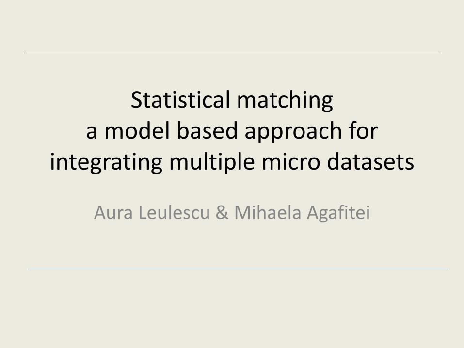
Introduction

• the same reference population

• the same reference period

• the same statistical unit

• Ideal framework to apply statistical matching techniques: nested surveys

Donor survey Recipient survey Synthetic dataset

X,Y

X,Z

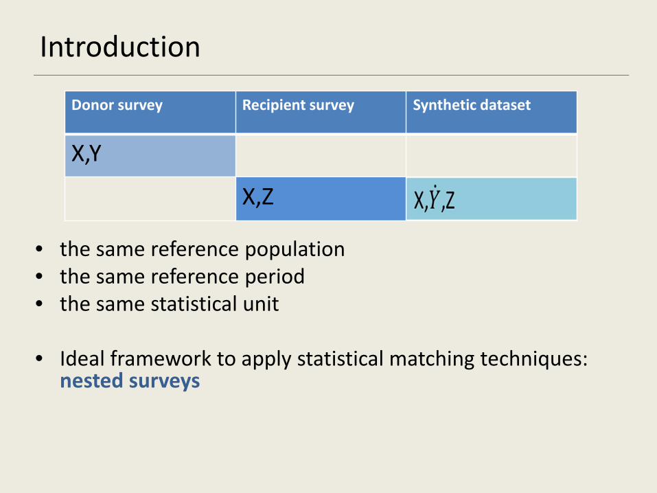
SM – a stepwise process

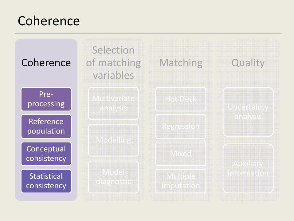
Coherence

Pre-processing

Reference population

Conceptual consistency

Statistical consistency

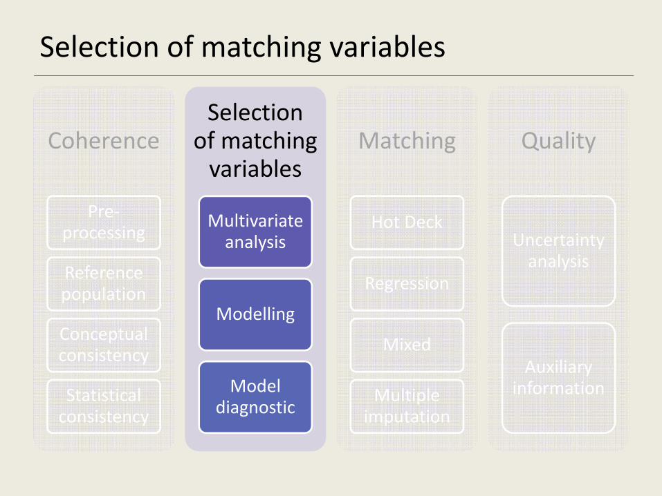
Selection of matching

variables

Multivariate analysis

Modelling

Model diagnostic

Matching

Hot Deck

Regression

Mixed

Multiple imputation

Quality

Uncertainty analysis

Auxiliary information

Coherence

Coherence

Pre-processing

Reference population

Conceptual consistency

Statistical consistency

Selectionof matching

variables

Multivariate analysis

Modelling

Model diagnostic

Matching

Hot Deck

Regression

Mixed

Multiple imputation

Quality

Uncertainty analysis

Auxiliary information

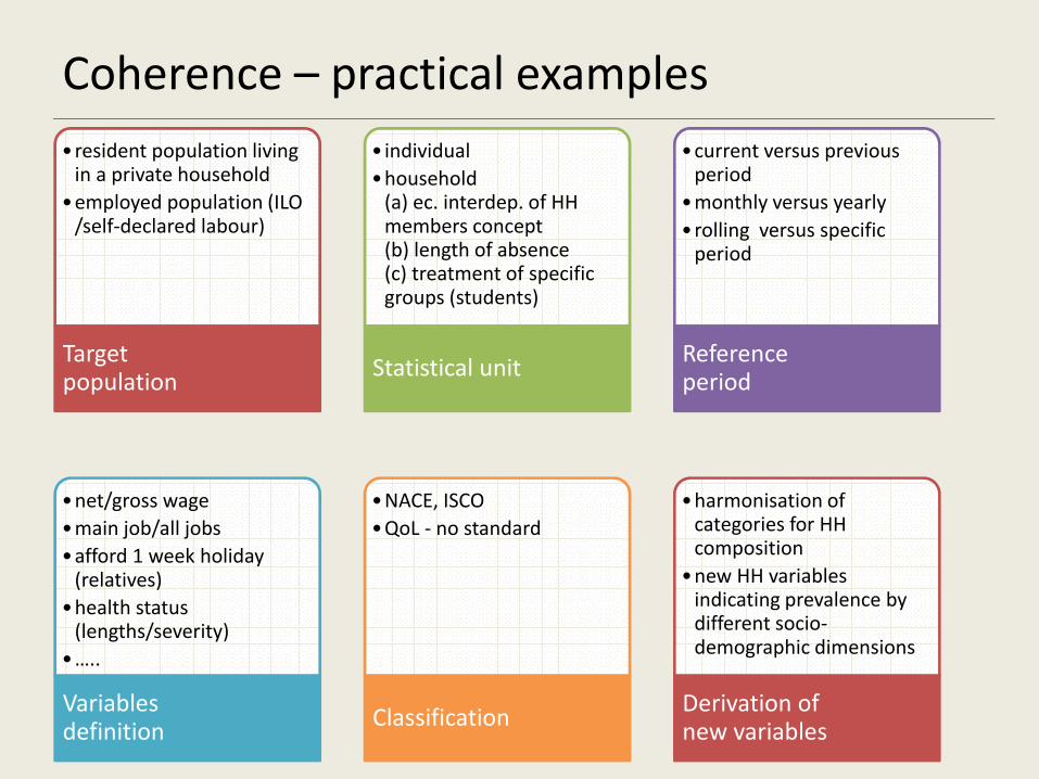
Coherence – practical examples

•resident population living in a private household

•employed population (ILO /self-declared labour)

Target population

•individual

•household(a) ec. interdep. of HH members concept (b) length of absence (c) treatment of specific groups (students)

Statistical unit

•current versus previous period

•monthly versus yearly

•rolling versus specific period

Reference period

•net/gross wage

•main job/all jobs

•afford 1 week holiday (relatives)

•health status (lengths/severity)

•…..

Variables definition

•NACE, ISCO

•QoL - no standard

Classification

•harmonisation of categories for HH composition

•new HH variables indicating prevalence by different socio-demographic dimensions

Derivation of new variables

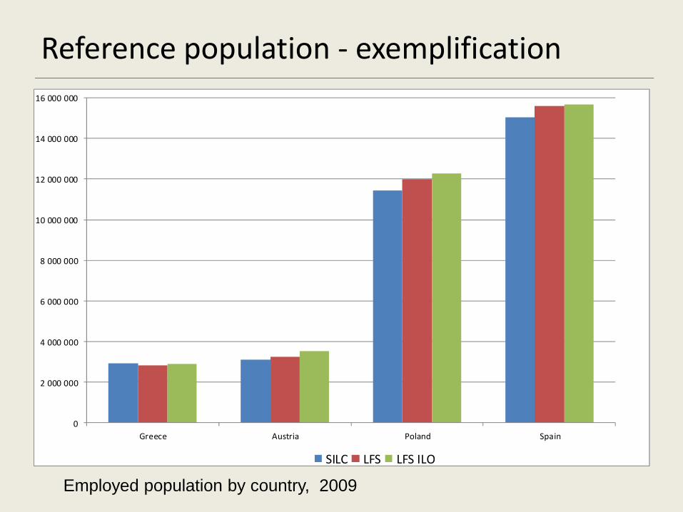
Reference population - exemplification

Employed population by country, 2009

0

2 000 000

4 000 000

6 000 000

8 000 000

10 000 000

12 000 000

14 000 000

16 000 000

Greece Austria Poland Spain

SILC LFS LFS ILO

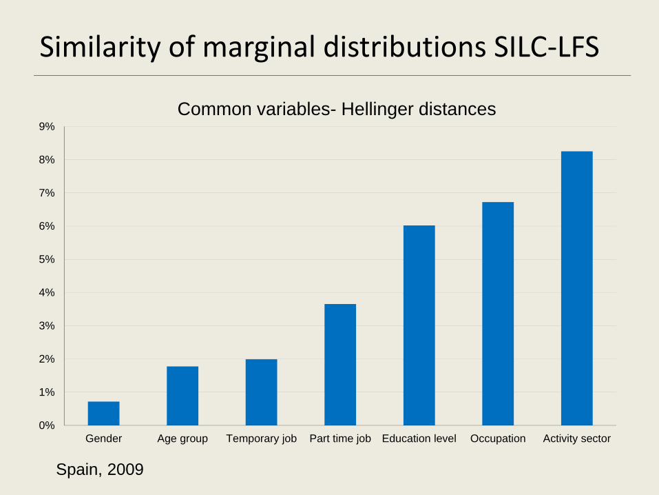
Similarity of marginal distributions SILC-LFS

Spain, 2009

0%

1%

2%

3%

4%

5%

6%

7%

8%

9%

Gender Age group Temporary job Part time job Education level Occupation Activity sector

Common variables- Hellinger distances

Selection of matching variables

Coherence

Pre-processing

Reference population

Conceptual consistency

Statistical consistency

Selection of matching

variables

Multivariate analysis

Modelling

Model diagnostic

Matching

Hot Deck

Regression

Mixed

Multiple imputation

Quality

Uncertainty analysis

Auxiliary information

Selection of matching variables

Common variables of high quality

no errors and missing

data

Coherent common variables at data and metadata level

ref. period, def., coverage, measurement unit, similar distribution

donor/ recipient

High explanatory power

correlations, regressions, model diagnostics

• The choice of matching variables is a crucial point in

statistical matching

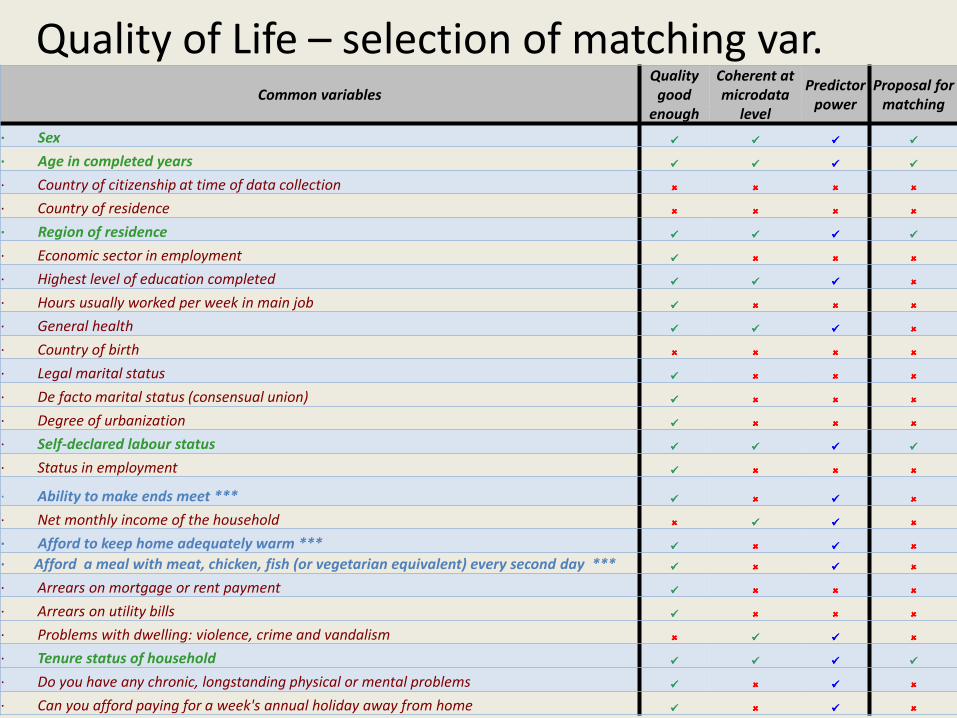
Quality of Life – selection of matching var.Common variables

Quality

good

enough

Coherent at

microdata

level

Predictor

power

Proposal for

matching

· Sex ���� ���� ���� ����

· Age in completed years ���� ���� ���� ����

· Country of citizenship at time of data collection ���� ���� ���� ����

· Country of residence ���� ���� ���� ����

· Region of residence ���� ���� ���� ����

· Economic sector in employment ���� ���� ���� ����

· Highest level of education completed ���� ���� ���� ����

· Hours usually worked per week in main job ���� ���� ���� ����

· General health ���� ���� ���� ����

· Country of birth ���� ���� ���� ����

· Legal marital status ���� ���� ���� ����

· De facto marital status (consensual union) ���� ���� ���� ����

· Degree of urbanization ���� ���� ���� ����

· Self-declared labour status ���� ���� ���� ����

· Status in employment ���� ���� ���� ����

· Ability to make ends meet *** ���� ���� ���� ����

· Net monthly income of the household ���� ���� ���� ����

· Afford to keep home adequately warm *** ���� ���� ���� � � � �

· Afford a meal with meat, chicken, fish (or vegetarian equivalent) every second day *** ���� ���� ���� ����

· Arrears on mortgage or rent payment ���� ���� ���� ����

· Arrears on utility bills ���� ���� ���� ����

· Problems with dwelling: violence, crime and vandalism ���� ���� ���� ����

· Tenure status of household ���� ���� ���� ����

· Do you have any chronic, longstanding physical or mental problems ���� ���� ���� ����

· Can you afford paying for a week's annual holiday away from home ���� ���� ���� ����

Log wage estimates using SILC dataVariable Coeff Standard

Error p-value

Intercept 6.422 0.001 <.0001 Age 0.001 0.008 <.0001 Age-square -0.000 0.001 <.0001 Male 0.124 0.001 <.0001 Isced2 0.131 0.0005 <.0001 Isced3 0.264 0.0009 <.0001 Isced4 0.354 0.0017 <.0001 Isced5 0.433 0.0019 <.0001 Isced6 0.506 0.0026 <.0001 Born EU -0.071 0.0005 <.0001 Born non EU -0.063 0.0003 <.0001 Densely populated 0.055 0.0002 <.0001 Intermediate populated 0.040 0.0002 <.0001 Married 0.067 0.0002 <.0001 Widowed/separated 0.018 0.0007 <.0001 Part time -0.464 0.0003 <.0001 Temporary job -0.114 0.0002 <.0001 Supervisory position 0.122 0.0002 <.0001 Firm size -0.112 0.0001 <.0001 Manufacturing 0.125 0.0006 <.0001 Electricity 0.214 0.001 <.0001 Construction 0.164 0.0007 <.0001 Public administration 0.181 0.0003 <.0001 Fin & insurance

0.224 0.0005 <.0001

Managers 0.356 0.0025 <.0001 Professionals 0.077 0.0035 <.0001 Technicians 0.096 0.0010 <.0001 Clerical workers 0.119 0.0008 <.0001 Service and sales 0.036 0.0007 <.0001 Skilled agricultural -0.029 0.001 <.0001 Craft 0.065 0.0007 <.0001 Plant and machine 0.042 0.0009 <.0001

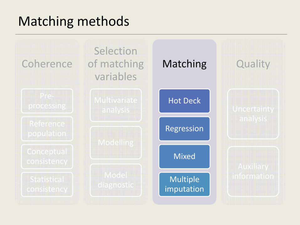
Matching methods

Coherence

Pre-processing

Reference population

Conceptual consistency

Statistical consistency

Selection of matching

variables

Multivariate analysis

Modelling

Model diagnostic

Matching

Hot Deck

Regression

Mixed

Multiple imputation

Quality

Uncertainty analysis

Auxiliary information

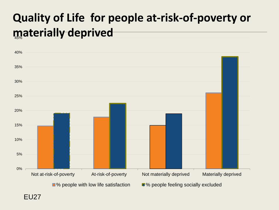
Quality of Life for people at-risk-of-poverty or

materially deprived

EU27

0%

5%

10%

15%

20%

25%

30%

35%

40%

45%

Not at-risk-of-poverty At-risk-of-poverty Not materially deprived Materially deprived

% people with low life satisfaction % people feeling socially excluded

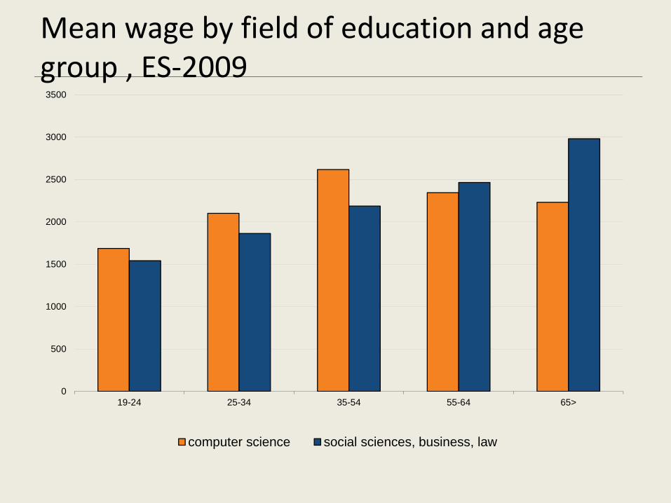
Mean wage by field of education and age

group , ES-2009

0

500

1000

1500

2000

2500

3000

3500

19-24 25-34 35-54 55-64 65>

computer science social sciences, business, law

Quality

Coherence

Pre-processing

Reference population

Conceptual consistency

Statistical consistency

Selection of matching

variables

Multivariate analysis

Modelling

Model diagnostic

Matching

Hot Deck

Regression

Mixed

Multiple imputation

Quality

Preservation distributions

Uncertainty analysis

Auxiliary information

Quality in SM –1st level

• Compare distributions imputed variables

• Compare joint distributions of imputed variables

and dimensions controlled in the model

– Easy to implement

– Good results when preconditions are met and

imputation procedures are robust

Preservation of distributions and main parameters (donor/recipient)

1st level of quality in SM

Preservation distributions EQLS observed-SILC imputed

Imputed Observed

0%

5%

10%

15%

20%

25%

30%

35%

Job satisfactionLife satisfactionTrust in othersTrust in government

0%

5%

10%

15%

20%

25%

30%

35%

Job satisfaction

Life satisfaction

Trust in others

Trust in government

Quality of Life, ES, 2007

1st level of quality in SM

Preservation distributions: cut-off points wage deciles

500

1000

1500

2000

2500

3000

1 2 3 4 5 6 7 8 9 10

LFS IMPUTED SILC CALIBRATED

19Wage, ES 2009

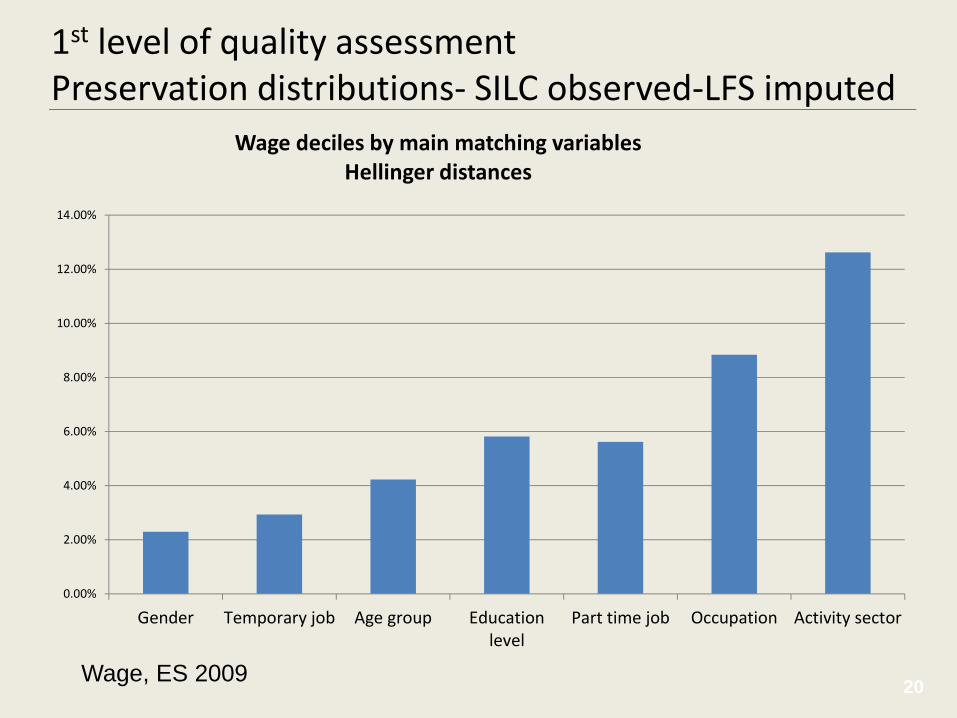
1st level of quality assessment

Preservation distributions- SILC observed-LFS imputed

20Wage, ES 2009

0.00%

2.00%

4.00%

6.00%

8.00%

10.00%

12.00%

14.00%

Gender Temporary job Age group Education

level

Part time job Occupation Activity sector

Wage deciles by main matching variables

Hellinger distances

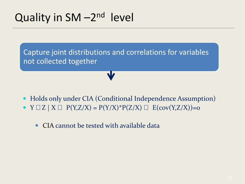
Quality in SM –2nd level

Capture joint distributions and correlations for variables not collected together

� Holds only under CIA (Conditional Independence Assumption)

� Y ⊥ Z | X ⇔ P(Y,Z/X) = P(Y/X)*P(Z/X) ⇔ E(cov(Y,Z/X))=0

� CIA cannot be tested with available data

21

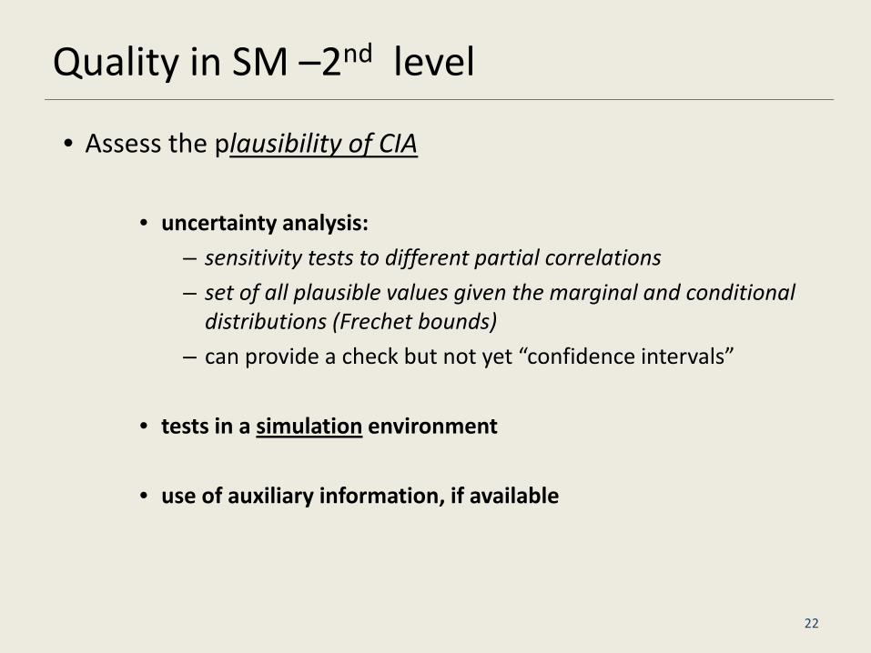
• Assess the plausibility of CIA

• uncertainty analysis:

– sensitivity tests to different partial correlations

– set of all plausible values given the marginal and conditional

distributions (Frechet bounds)

– can provide a check but not yet “confidence intervals”

• tests in a simulation environment

• use of auxiliary information, if available

22

Quality in SM –2nd level

2nd level of quality in SM

JOINT distributions (Frechet Bounds)

ES 2009

0%

5%

10%

15%

20%

25%

30%

% people with wage below mean

by field of education

low bound CIA high bound

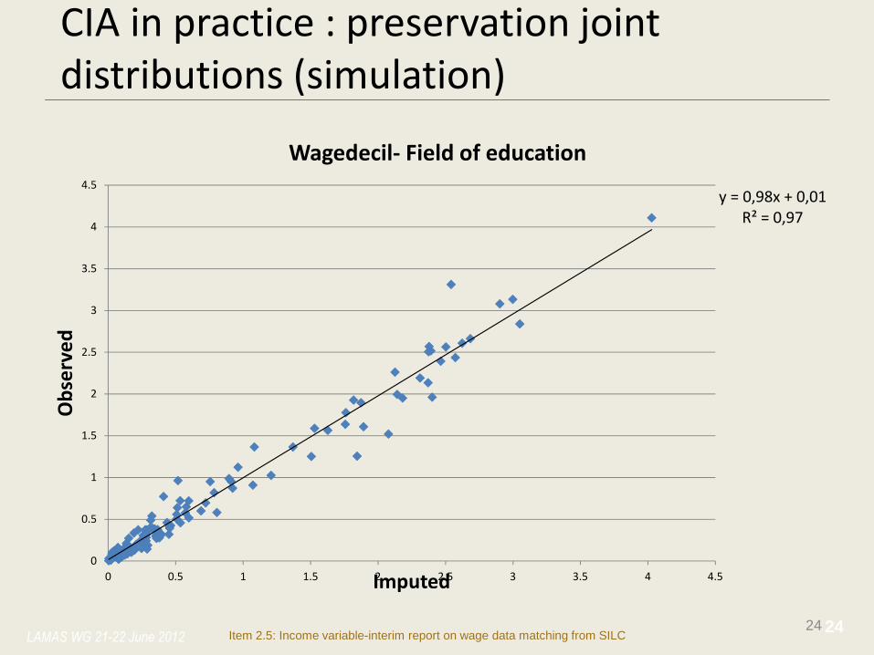
CIA in practice : preservation joint

distributions (simulation)

24

y = 0,98x + 0,01

R² = 0,97

0

0.5

1

1.5

2

2.5

3

3.5

4

4.5

0 0.5 1 1.5 2 2.5 3 3.5 4 4.5

Ob

serv

ed

Imputed

Wagedecil- Field of education

LAMAS WG 21-22 June 2012 Item 2.5: Income variable-interim report on wage data matching from SILC24

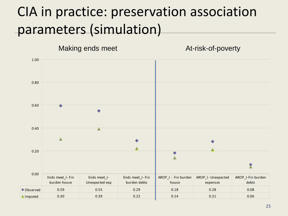
CIA in practice: preservation association

parameters (simulation)

0.00

0.20

0.40

0.60

0.80

1.00

Observed 0.59 0.55 0.29 0.18 0.28 0.08

Imputed 0.30 0.39 0.22 0.14 0.21 0.06

Ends meet_I- Fin

burden house

Ends meet_I-

Unexpected exp

Ends meet_I- Fin

burden debts

AROP_I - Fin burden

house

AROP_I- Unexpected

expenses

AROP_I-Fin burden

debts

25

Making ends meet At-risk-of-poverty

CIA in practice: mediated effects

X (matchingvariables)

Z (targetvariable)

Y (targetvariable)

01=β

effectindirect

XZY

ZY

_1

21

=−+++=

++=

ββεββα

εβα

CIA in practice: conclusions

• CIA leads very often to an underestimation of correlations

• Essential to identify the target variables in both surveys

– Focus on ‘joint information’ between specific variables

• Matching should provide

– ‘relevant’ results: Y and Z correlated

– ‘reliable’ results: the correlation should be mediated to a large extent by Xs

• Quality measures

– uncertainty measures (Frechet bounds)

– variance estimation (multiple imputation with different partial correlations)

27

Relax the CIA: use of auxiliary information

• Proxy variables

– extend the set of matching variables

– add ‘hook variables’- e.g. net monthly income

– latent classes: CIA holds within certain segments of

population

» Specific purpose

• Third datasets/Overlaps of samples

– split questionnaire design

– every combination of variables is observed in one sub-

sample

– Precision estimates based on multiple imputation

» Synthetic datasets

28

Conclusions

• better coherence is an essential step for SM

• external data sources: lack of harmonization and quality

problems

• quality needs a process approach

– need to consider implicit assumptions

• from ex-post to ex ante:

– Possibility to address current limitations in the design

phase

• auxiliary information

• identify cases when implicit assumptions hold

– More systematic approach

– Consider jointly with linking from administrative sources

29