Embed Size (px)
Citation preview
Statistical Issues in the Use of CompositeEndpoints in Clinical Trials
Longyang Wu and Richard Cook
Statistics and Actuarial Science, University of Waterloo
May 14, 2010
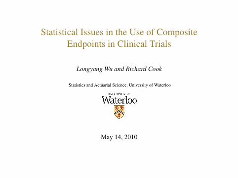
Outline
Introduction:A brief overview of composite endpoints in clinical trials.
Composite Endpoint Analysis: Time-to-First-EventA Cox Model For Composite Endpoints:
Independent ComponentsAssociated ComponentsTreatment Effects: What Are We Estimating?
Empirical Study I
A Global Analysis: A Multivariate ApproachA Marginal Approach to Multivariate Event Data
Global Treatment Effect Estimation: Interpretation?
Empirical Study II
A Real Data ExampleComments From Clinical LiteratureDiscussion
2 / 53
COMPOSITE ENDPOINTS
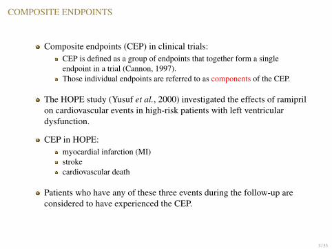
Composite endpoints (CEP) in clinical trials:CEP is defined as a group of endpoints that together form a singleendpoint in a trial (Cannon, 1997).Those individual endpoints are referred to as components of the CEP.
The HOPE study (Yusuf et al., 2000) investigated the effects of ramiprilon cardiovascular events in high-risk patients with left ventriculardysfunction.
CEP in HOPE:myocardial infarction (MI)strokecardiovascular death
Patients who have any of these three events during the follow-up areconsidered to have experienced the CEP.
3 / 53
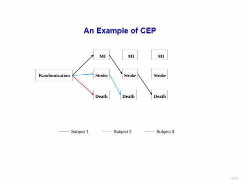
Randomization
MI MI MI
Stroke Stroke
Death
Stroke
Death Death
Subject 1 Subject 2 Subject 3
4 / 53
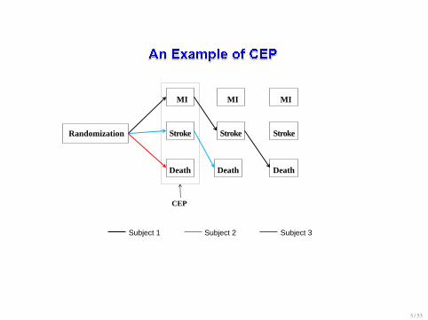
Randomization
MI MI MI
Stroke Stroke
Death
Stroke
Death Death
CEP
Subject 1 Subject 2 Subject 3
5 / 53

Our Present Objectives
The focus of this study will be on CEP of time event data.
We used models, asymptotic theory and empirical studies formallyinvestigate the behaviour of estimation of treatment effects.
Use simulations to study the implications of using CEP in the statisticalpower and sample size requirement.
Investigate the validity of some of recommendations of CEP analysis.
Study the effectiveness of alternative design and analysis
6 / 53

Counting Process Notation: Review of Univariate Failure Times
Let Ti be the time to the CEP with Ni(t) = I(Ti 6 t) and processhistoryHi(t) = {Ni(u), Zi, 0 < u < t}.Let ∆Ni(t) = Ni(t+ ∆t−)−Ni(t−) and dNi(t) = lim∆t↓0 ∆Ni(t).The hazard function for Ti is defined as
λi(t|Hi(t)) = E (dNi(t)|Hi(t)) = lim∆t↓0
P (∆Ni(t) = 1|Hi(t))∆t
where E (·) denotes the expectation operator with respect to the trueprocess history.
7 / 53
Counting Process Notation: Review of Univariate Failure Times
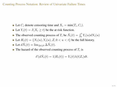
Let Ci denote censoring time and Xi = min(Ti, Ci).Let Yi(t) = I(Xi ≥ t) be the at risk function.
The observed counting process of Ti be Ni(t) =∫ t
0Yi(u)dNi(u)
Let Hi(t) = {Ni(u), Yi(u), Z, 0 < u < t} be the full history.Let dNi(t) = lim∆t↓0 ∆Ni(t).The hazard of the observed counting process of Ti is
E (dNi(t) = 1|Hi(t)) = Yi(t)λ(t|Zi)dt.
8 / 53
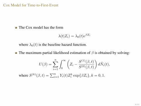
Cox Model for Time-to-First-Event
The Cox model has the form
λ(t|Zi) = λ0(t)eβZi
where λ0(t) is the baseline hazard function.
The maximum partial likelihood estimation of β is obtained by solving:
U(β) =
n∑i=1
∫ ∞0
(Zi −
S(1)(β, t)
S(0)(β, t)
)dNi(t),
where S(k)(β, t) =∑ni=1 Yi(t)Z
ki exp{βZi}, k = 0, 1.
9 / 53
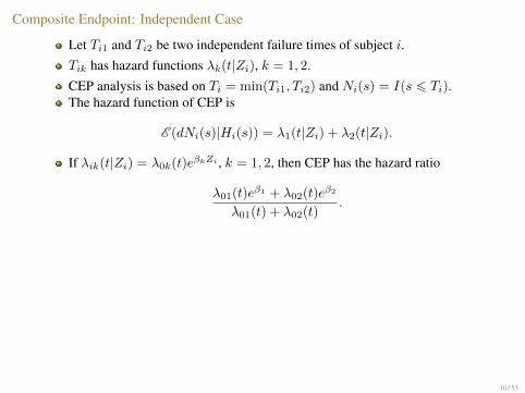
Composite Endpoint: Independent Case
Let Ti1 and Ti2 be two independent failure times of subject i.Tik has hazard functions λk(t|Zi), k = 1, 2.
CEP analysis is based on Ti = min(Ti1, Ti2) and Ni(s) = I(s 6 Ti).The hazard function of CEP is
E (dNi(s)|Hi(s)) = λ1(t|Zi) + λ2(t|Zi).
If λik(t|Zi) = λ0k(t)eβkZi , k = 1, 2, then CEP has the hazard ratio
λ01(t)eβ1 + λ02(t)eβ2
λ01(t) + λ02(t).
Remarks:1.The proportional hazard assumption holds for CEP, if
(A.1) β1 = β2: the same treatment effect across components, or(A.2) λ01(t) = λ02(t): the same frequency of occurrence.
2. Otherwise, PH does not hold for CEP analysis.
What are we estimating in this case?
10 / 53

Composite Endpoint: Independent Case
Let Ti1 and Ti2 be two independent failure times of subject i.Tik has hazard functions λk(t|Zi), k = 1, 2.
CEP analysis is based on Ti = min(Ti1, Ti2) and Ni(s) = I(s 6 Ti).The hazard function of CEP is
E (dNi(s)|Hi(s)) = λ1(t|Zi) + λ2(t|Zi).
If λik(t|Zi) = λ0k(t)eβkZi , k = 1, 2, then CEP has the hazard ratio
λ01(t)eβ1 + λ02(t)eβ2
λ01(t) + λ02(t).
Remarks:1.The proportional hazard assumption holds for CEP, if
(A.1) β1 = β2: the same treatment effect across components, or(A.2) λ01(t) = λ02(t): the same frequency of occurrence.
2. Otherwise, PH does not hold for CEP analysis.
What are we estimating in this case?
11 / 53

Composite Endpoint: Independent Case
Let Ti1 and Ti2 be two independent failure times of subject i.Tik has hazard functions λk(t|Zi), k = 1, 2.
CEP analysis is based on Ti = min(Ti1, Ti2) and Ni(s) = I(s 6 Ti).The hazard function of CEP is
E (dNi(s)|Hi(s)) = λ1(t|Zi) + λ2(t|Zi).
If λik(t|Zi) = λ0k(t)eβkZi , k = 1, 2, then CEP has the hazard ratio
λ01(t)eβ1 + λ02(t)eβ2
λ01(t) + λ02(t).
Remarks:1.The proportional hazard assumption holds for CEP, if
(A.1) β1 = β2: the same treatment effect across components, or(A.2) λ01(t) = λ02(t): the same frequency of occurrence.
2. Otherwise, PH does not hold for CEP analysis.
What are we estimating in this case?
12 / 53
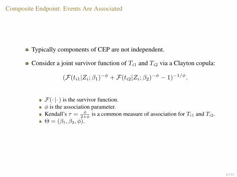
Composite Endpoint: Events Are Associated
Typically components of CEP are not independent.
Consider a joint survivor function of Ti1 and Ti2 via a Clayton copula:
(F(ti1|Zi;β1)−φ + F(ti2|Zi;β2)−φ − 1)−1/φ.
F(· |· ) is the survivor function.φ is the association parameter.Kendall’s τ = φ
2+φis a common measure of association for Ti1 and Ti2.
Θ = (β1, β2, φ).
13 / 53
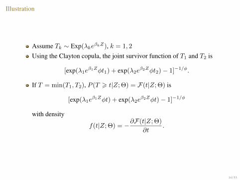
Illustration
Assume Tk ∼ Exp(λkeβkZ), k = 1, 2
Using the Clayton copula, the joint survivor function of T1 and T2 is
[exp(λ1eβ1Zφt1) + exp(λ2e
β2Zφt2)− 1]−1/φ.
If T = min(T1, T2), P (T > t|Z; Θ) = F(t|Z; Θ) is
[exp(λ1eβ1Zφt) + exp(λ2e
β2Zφt)− 1]−1/φ
with density
f(t|Z; Θ) = −∂F(t|Z; Θ)
∂t.
14 / 53

Composite endpoint: Correlated Components
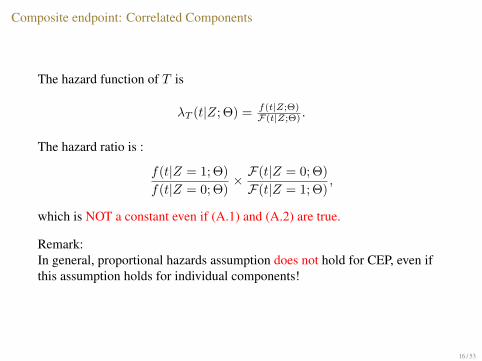
The hazard function of T is
λT (t|Z; Θ) = f(t|Z;Θ)F(t|Z;Θ) .
The hazard ratio is :
f(t|Z = 1; Θ)
f(t|Z = 0; Θ)× F(t|Z = 0; Θ)
F(t|Z = 1; Θ),
which is NOT a constant even if (A.1) and (A.2) are true.
Remark:In general, proportional hazards assumption does not hold for CEP, even ifthis assumption holds for individual components!
15 / 53
Composite endpoint: Correlated Components
The hazard function of T is
λT (t|Z; Θ) = f(t|Z;Θ)F(t|Z;Θ) .
The hazard ratio is :
f(t|Z = 1; Θ)
f(t|Z = 0; Θ)× F(t|Z = 0; Θ)
F(t|Z = 1; Θ),
which is NOT a constant even if (A.1) and (A.2) are true.
Remark:In general, proportional hazards assumption does not hold for CEP, even ifthis assumption holds for individual components!
16 / 53
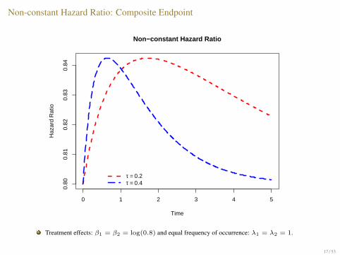
Non-constant Hazard Ratio: Composite Endpoint
0 1 2 3 4 5
0.80
0.81
0.82
0.83
0.84
Non−constant Hazard Ratio
Time
Haz
ard
Rat
io
τ = 0.2τ = 0.4
Treatment effects: β1 = β2 = log(0.8) and equal frequency of occurrence: λ1 = λ2 = 1.
17 / 53
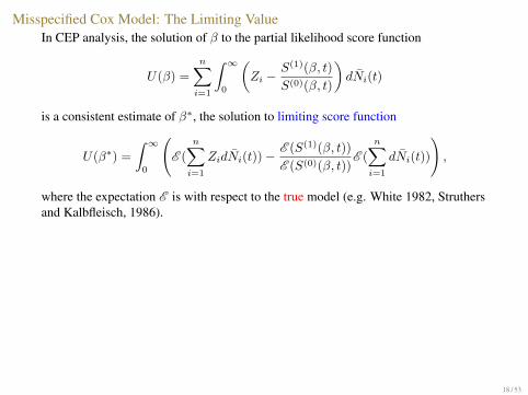
Misspecified Cox Model: The Limiting ValueIn CEP analysis, the solution of β to the partial likelihood score function
U(β) =n∑i=1
∫ ∞0
(Zi −
S(1)(β, t)
S(0)(β, t)
)dNi(t)
is a consistent estimate of β∗, the solution to limiting score function
U(β∗) =
∫ ∞0
(E (
n∑i=1
ZidNi(t))−E (S(1)(β, t))
E (S(0)(β, t))E (
n∑i=1
dNi(t))
),
where the expectation E is with respect to the true model (e.g. White 1982, Struthersand Kalbfleisch, 1986).
Remark: β∗ 6= β0.
18 / 53
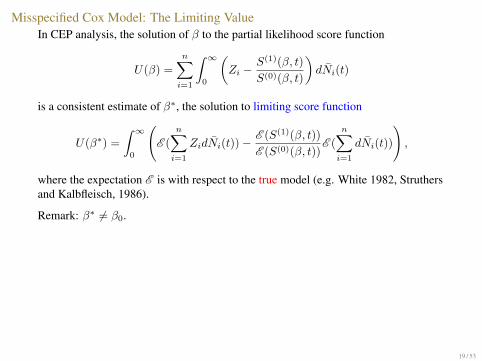
Misspecified Cox Model: The Limiting ValueIn CEP analysis, the solution of β to the partial likelihood score function
U(β) =n∑i=1
∫ ∞0
(Zi −
S(1)(β, t)
S(0)(β, t)
)dNi(t)
is a consistent estimate of β∗, the solution to limiting score function
U(β∗) =
∫ ∞0
(E (
n∑i=1
ZidNi(t))−E (S(1)(β, t))
E (S(0)(β, t))E (
n∑i=1
dNi(t))
),
where the expectation E is with respect to the true model (e.g. White 1982, Struthersand Kalbfleisch, 1986).
Remark: β∗ 6= β0.
19 / 53
Limiting Treatment Effect: The Independent Case
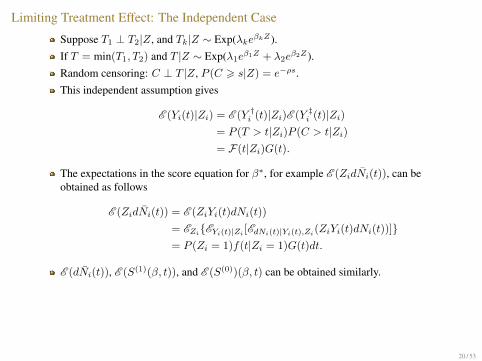
Suppose T1 ⊥ T2|Z, and Tk|Z ∼ Exp(λkeβkZ).If T = min(T1, T2) and T |Z ∼ Exp(λ1e
β1Z + λ2eβ2Z).
Random censoring: C ⊥ T |Z, P (C > s|Z) = e−ρs.This independent assumption gives
E (Yi(t)|Zi) = E (Y †i (t)|Zi)E (Y ‡i (t)|Zi)= P (T > t|Zi)P (C > t|Zi)= F(t|Zi)G(t).
The expectations in the score equation for β∗, for example E (ZidNi(t)), can beobtained as follows
E (ZidNi(t)) = E (ZiYi(t)dNi(t))
= EZi{EYi(t)|Zi[EdNi(t)|Yi(t),Zi
(ZiYi(t)dNi(t))]}= P (Zi = 1)f(t|Zi = 1)G(t)dt.
E (dNi(t)), E (S(1)(β, t)), and E (S(0))(β, t) can be obtained similarly.
20 / 53
Limiting Treatment Effect: The Independent Case
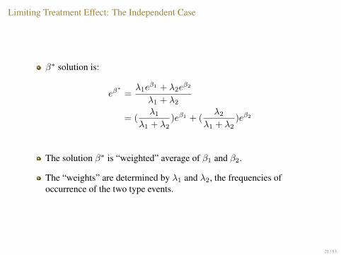
β∗ solution is:
eβ∗
=λ1e
β1 + λ2eβ2
λ1 + λ2
= (λ1
λ1 + λ2)eβ1 + (
λ2
λ1 + λ2)eβ2
The solution β∗ is “weighted” average of β1 and β2.
The “weights” are determined by λ1 and λ2, the frequencies ofoccurrence of the two type events.
21 / 53
Limiting treatment effect: Associated Components
Use Clayton Copula to model the association.
The solution of β∗ is obtained by numerical integration.
Some surprising observations on the relation between β∗ and β1, β2, φ.
22 / 53
Limiting Value: Dependent Case with Unequal Treatment Effect
0.2 0.4 0.6 0.8
0.85
0.90
0.95
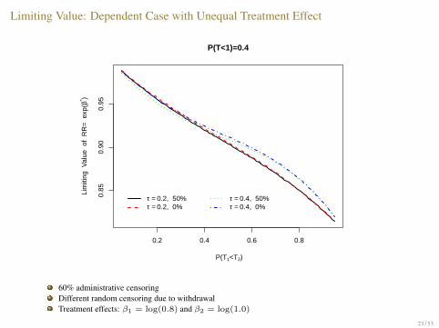
P(T<1)=0.4
P(T1<T2)
Lim
iting
Val
ue o
f R
R=
exp
(β* )
τ = 0.2, 50% τ = 0.2, 0%
τ = 0.4, 50% τ = 0.4, 0%
60% administrative censoringDifferent random censoring due to withdrawalTreatment effects: β1 = log(0.8) and β2 = log(1.0)
23 / 53
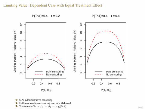
Limiting Value: Dependent Case with Equal Treatment Effect
0.2 0.4 0.6 0.8
02
46
810
12
P(T<1)=0.4, τ = 0.2
P(T1<T2)
Lim
iting
Per
cent
Rel
ativ
e B
ias
(%
)
50% censoringNo censoring
0.2 0.4 0.6 0.80
24
68
1012
P(T<1)=0.4, τ = 0.4
P(T1<T2)
Lim
iting
Per
cent
Rel
ativ
e B
ias
(%
) 50% censoringNo censoring
60% administrative censoringDifferent random censoring due to withdrawalTreatment effects: β1 = β2 = log(0.8) 24 / 53
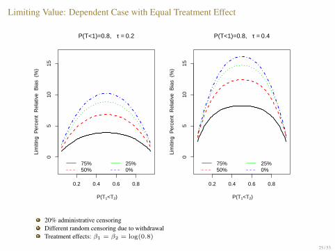
Limiting Value: Dependent Case with Equal Treatment Effect
0.2 0.4 0.6 0.8
05
1015
P(T<1)=0.8, τ = 0.2
P(T1<T2)
Lim
iting
Per
cent
Rel
ativ
e B
ias
(%
)
75%50%
25%0%
0.2 0.4 0.6 0.80
510
15
P(T<1)=0.8, τ = 0.4
P(T1<T2)
Lim
iting
Per
cent
Rel
ativ
e B
ias
(%
)75%50%
25%0%
20% administrative censoringDifferent random censoring due to withdrawalTreatment effects: β1 = β2 = log(0.8)
25 / 53
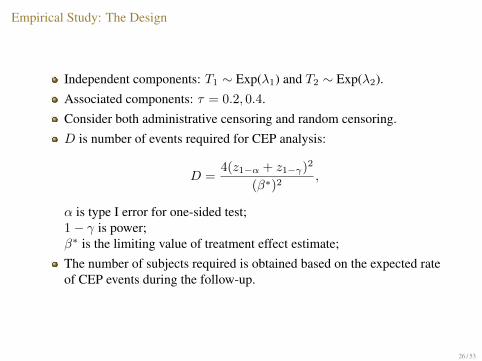
Empirical Study: The Design
Independent components: T1 ∼ Exp(λ1) and T2 ∼ Exp(λ2).Associated components: τ = 0.2, 0.4.Consider both administrative censoring and random censoring.D is number of events required for CEP analysis:
D =4(z1−α + z1−γ)2
(β∗)2,
α is type I error for one-sided test;1− γ is power;β∗ is the limiting value of treatment effect estimate;The number of subjects required is obtained based on the expected rateof CEP events during the follow-up.
26 / 53
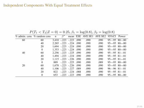
Independent Components With Equal Treatment Effects
P (T1 < T2|Z = 0) = 0.25, β1 = log(0.8), β2 = log(0.8)% admin. cens % random cens n β∗ mean ESE AVE SE1 AVE SE2 95%CI Power
60 60 3,410 -.223 -.223 .090 .090 .090 95—95 80—8040 2,265 -.223 -.224 .090 .090 .090 95—95 80—8020 1,694 -.223 -.224 .090 .090 .090 95—95 80—800 1,353 -.223 -.224 .090 .090 .090 95—95 80—80
40 60 2,256 -.223 -.225 .090 .090 .090 95—95 81—8140 1,494 -.223 -.224 .090 .090 .090 95—95 81—8120 1,115 -.223 -.226 .090 .090 .090 95—95 81—810 889 -.223 -.225 .090 .090 .089 95—95 80—80
20 60 1,678 -.223 -.226 .090 .090 .090 95—95 80—8040 1,106 -.223 -.227 .089 .090 .090 96—96 81—8120 822 -.223 -.224 .088 .090 .090 95—95 81—810 653 -.223 -.223 .090 .090 .090 95—95 80—80
27 / 53

Independent Component With Unequal Treatment Effect
P (T1 < T2|Z = 0) = 0.25, β1 = log(0.8), β2 = log(1.0)% admin cens % random cens n β∗ mean ESE AVE SE1 AVE SE2 95%CI Power
60 60 60,737 -.051 -.052 .020 .021 .021 96—96 82—8240 40,450 -.051 -.052 .021 .021 .021 95—95 81—8120 30,317 -.051 -.052 .021 .021 .021 95—95 81—810 24,241 -.051 -.052 .021 .021 .021 95—95 82—82
40 60 40,411 -.051 -.052 .021 .021 .021 95—95 80—8040 26,892 -.051 -.052 .021 .021 .021 95—95 81—8120 20,143 -.051 -.052 .021 .021 .021 95—95 82—820 16,099 -.051 -.052 .021 .021 .021 95—95 80—80
20 60 30,242 -.051 -.052 .021 .021 .021 95—95 80—8040 20,101 -.051 -.052 .021 .021 .021 95—95 82—8220 15,041 -.051 -.052 .021 .021 .021 94—94 81—810 12,011 -.051 -.052 .021 .021 .021 94—94 81—81
28 / 53
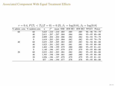
Associated Component With Equal Treatment Effects
τ = 0.4, P (T1 < T2|Z = 0) = 0.25, β1 = log(0.8), β2 = log(0.8)% admin. cens % random cens n β∗ mean ESE AVE SE1 AVE SE2 95%CI Power
60 60 3,825 -.210 -.210 .085 .085 .085 96—96 79—7940 2,611 -.207 -.207 .084 .084 .084 95—95 80—8020 2,009 -.204 -.204 .086 .082 .082 94—94 79—790 1,619 -.203 -.203 .084 .082 .082 95—95 79—79
40 60 2,653 -.205 -.205 .083 .083 .083 94—94 80—8040 1,825 -.201 -.202 .081 .081 .081 95—95 80—8020 1,402 -.198 -.199 .079 .080 .080 95—95 81—810 1,140 -.196 -.197 .079 .079 .079 95—95 80—80
20 60 2,033 -.202 -.203 .081 .082 .082 95—95 80—8040 1,393 -.198 -.199 .081 .080 .080 95—95 80—8020 1,056 -.196 -.197 .079 .079 .079 95—95 81—810 857 -.194 -.194 .077 .078 .078 95—95 80—80
29 / 53
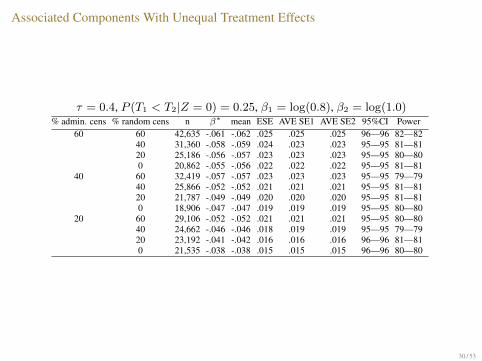
Associated Components With Unequal Treatment Effects
τ = 0.4, P (T1 < T2|Z = 0) = 0.25, β1 = log(0.8), β2 = log(1.0)% admin. cens % random cens n β∗ mean ESE AVE SE1 AVE SE2 95%CI Power
60 60 42,635 -.061 -.062 .025 .025 .025 96—96 82—8240 31,360 -.058 -.059 .024 .023 .023 95—95 81—8120 25,186 -.056 -.057 .023 .023 .023 95—95 80—800 20,862 -.055 -.056 .022 .022 .022 95—95 81—81
40 60 32,419 -.057 -.057 .023 .023 .023 95—95 79—7940 25,866 -.052 -.052 .021 .021 .021 95—95 81—8120 21,787 -.049 -.049 .020 .020 .020 95—95 81—810 18,906 -.047 -.047 .019 .019 .019 95—95 80—80
20 60 29,106 -.052 -.052 .021 .021 .021 95—95 80—8040 24,662 -.046 -.046 .018 .019 .019 95—95 79—7920 23,192 -.041 -.042 .016 .016 .016 96—96 81—810 21,535 -.038 -.038 .015 .015 .015 96—96 80—80
30 / 53
Multivariate Time-to-Event Analysis: A Marginal Approach
The Marginal Model of Wei, Lin, and Weissfeld (1989):Model-free to the dependence structure among the multivariate failuretimes, i.e., components in CEP.Fit ordinary Cox model to each component and estimate the regressioncoefficients.Use robust variance estimate in inference to account for possiblecorrelation in the data.
Advantages:Can be easily implemented in R or SAS.Affords great flexibility in formation of strata and risk sets.Well-developed variance estimator—Robust Variance Estimator.
31 / 53

Comparison of Multivariate Analysis and CEP
Time since randomization
Endpoint 1
Endpoint 2
Endpoint 3
CensoringCEP = 1 event
32 / 53
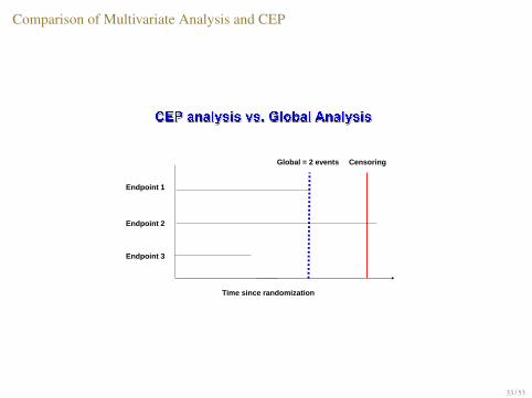
Comparison of Multivariate Analysis and CEP
Time since randomization
Endpoint 1
Endpoint 2
Endpoint 3
CensoringGlobal = 2 events
33 / 53
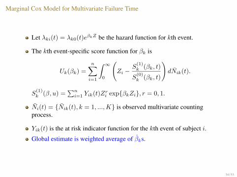
Marginal Cox Model for Multivariate Failure Time
Let λki(t) = λk0(t)eβkZ be the hazard function for kth event.
The kth event-specific score function for βk is
Uk(βk) =
n∑i=1
∫ ∞0
(Zi −
S(1)k (βk, t)
S(0)k (βk, t)
)dNik(t).
S(1)k (β, u) =
∑ni=1 Yik(t)Zri exp{βkZi}, r = 0, 1.
Ni(t) = {Nik(t), k = 1, ...,K} is observed multivariate countingprocess.
Yik(t) is the at risk indicator function for the kth event of subject i.
Global estimate is weighted average of βks.
34 / 53

Empirical Study II: Associated Components With Equal Treatment Effects
τ = 0.4, P (T1 < T2|Z = 0) = 0.25, β1 = log(0.8), β2 = log(0.8)%admin. cens % random cens n β∗ mean ESE AVE SE 95%CI Power
60 60 3,387 -.223 -.224 .091 .09 95 8040 2,247 -.223 -.224 .089 .09 95 8120 1,679 -.223 -.225 .091 .09 94 810 1,340 -.223 -.224 .09 .089 95 80
40 60 2,239 -.223 -.225 .091 .09 96 8040 1,481 -.223 -.224 .088 .089 95 8120 1,104 -.223 -.225 .086 .088 96 820 879 -.223 -.225 .085 .088 96 82
20 60 1,666 -.223 -.225 .088 .089 96 8240 1,097 -.223 -.225 .088 .088 95 8120 815 -.223 -.224 .086 .087 95 830 648 -.223 -.223 .086 .086 95 83
35 / 53
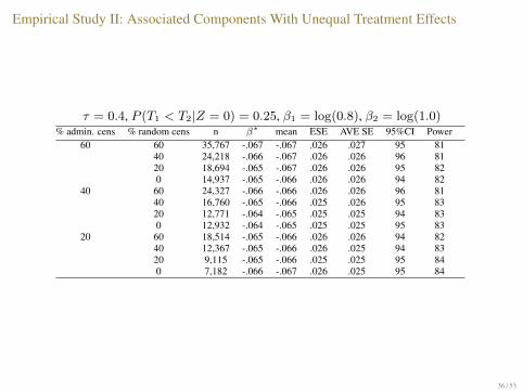
Empirical Study II: Associated Components With Unequal Treatment Effects
τ = 0.4, P (T1 < T2|Z = 0) = 0.25, β1 = log(0.8), β2 = log(1.0)% admin. cens % random cens n β∗ mean ESE AVE SE 95%CI Power
60 60 35,767 -.067 -.067 .026 .027 95 8140 24,218 -.066 -.067 .026 .026 96 8120 18,694 -.065 -.067 .026 .026 95 820 14,937 -.065 -.066 .026 .026 94 82
40 60 24,327 -.066 -.066 .026 .026 96 8140 16,760 -.065 -.066 .025 .026 95 8320 12,771 -.064 -.065 .025 .025 94 830 12,932 -.064 -.065 .025 .025 95 83
20 60 18,514 -.065 -.066 .026 .026 94 8240 12,367 -.065 -.066 .026 .025 94 8320 9,115 -.065 -.066 .025 .025 95 840 7,182 -.066 -.067 .026 .025 95 84
36 / 53

Sample Size Requirement: Global vs CEP
60% admin. cens., τ = 0.4, P (T1 < T2|Z = 0) = 0.25,β1 = log(0.8), β2 = log(0.8)
Random Censoring
Sam
ple
Siz
e
0
1000
2000
3000
4000
60% 40% 20% 0%
Global
CEP
37 / 53
A Real Data Example
An asthma management study—an experimental intervention wastested to delay the time to exacerbation.
Two endpoints:Endpoint I: severe exacerbation.Endpoint II: mild exacerbation.
CEP: time to the first event of endpoint I or II.
38 / 53
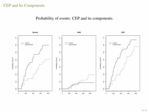
CEP and Its Components
Probability of events: CEP and its components.
0 200 400 600 800
0.0
0.1
0.2
0.3
0.4
0.5
0.6
0.7
Severe
Pro
babi
lity
of E
vent
ControlExperimental
0 200 400 600 800
0.0
0.1
0.2
0.3
0.4
0.5
0.6
0.7
Mild
Pro
babi
lity
of E
vent
ControlExperimental
0 200 400 600 800
0.0
0.1
0.2
0.3
0.4
0.5
0.6
0.7
CEP
Pro
babi
lity
of E
vent
ControlExperimental
39 / 53
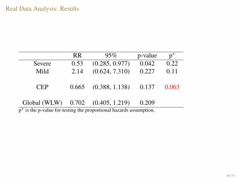
Real Data Analysis: Results
RR 95% p-value p∗
Severe 0.53 (0.285, 0.977) 0.042 0.22Mild 2.14 (0.624, 7.310) 0.227 0.11
CEP 0.665 (0.388, 1.138) 0.137 0.063
Global (WLW) 0.702 (0.405, 1.219) 0.209p∗ is the p-value for testing the proportional hazards assumption.
40 / 53
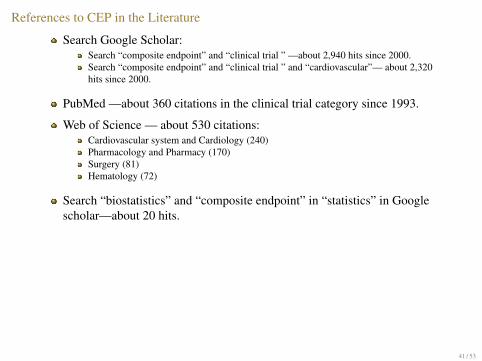
References to CEP in the Literature
Search Google Scholar:Search “composite endpoint” and “clinical trial ” —about 2,940 hits since 2000.Search “composite endpoint” and “clinical trial ” and “cardiovascular”— about 2,320hits since 2000.
PubMed —about 360 citations in the clinical trial category since 1993.
Web of Science — about 530 citations:Cardiovascular system and Cardiology (240)Pharmacology and Pharmacy (170)Surgery (81)Hematology (72)
Search “biostatistics” and “composite endpoint” in “statistics” in Googlescholar—about 20 hits.
41 / 53
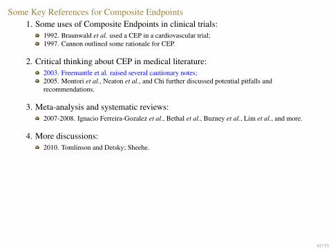
Some Key References for Composite Endpoints1. Some uses of Composite Endpoints in clinical trials:
1992. Braunwald et al. used a CEP in a cardiovascular trial;1997. Cannon outlined some rationale for CEP.
2. Critical thinking about CEP in medical literature:2003. Freemantle et al. raised several cautionary notes;2005. Montori et al., Neaton et al., and Chi further discussed potential pitfalls andrecommendations.
3. Meta-analysis and systematic reviews:2007-2008. Ignacio Ferreira-Gozalez et al., Bethal et al., Buzney et al., Lim et al., and more.
4. More discussions:2010. Tomlinson and Detsky; Sheehe.
42 / 53
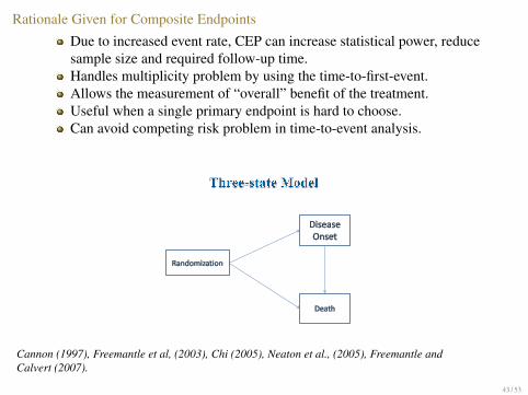
Rationale Given for Composite Endpoints
Due to increased event rate, CEP can increase statistical power, reducesample size and required follow-up time.Handles multiplicity problem by using the time-to-first-event.Allows the measurement of “overall” benefit of the treatment.Useful when a single primary endpoint is hard to choose.Can avoid competing risk problem in time-to-event analysis.
43 / 53
Cannon (1997), Freemantle et al, (2003), Chi (2005), Neaton et al., (2005), Freemantle andCalvert (2007).

Reported Limitations of Composite Endpoints
Heterogeneity in the treatment effect across components:Poor power for detecting heterogeneity.Interpretation of treatment effect can be difficult.
Importance of the components may not be equal at the patient level,e.g. TIA, stroke, MI, death.
44 / 53
Freemantle et al, (2003), Neaton et al., (2005), Montori et al., (2005), Freemantle and Calvert(2007).
Recommendations Regarding Composite Endpoints
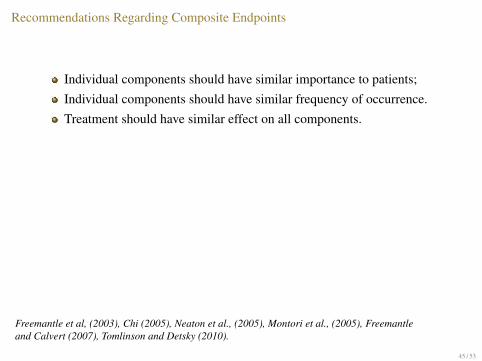
Individual components should have similar importance to patients;Individual components should have similar frequency of occurrence.Treatment should have similar effect on all components.
The last two may not be good recommendations:Largest bias when components are associated!
Data from all components should be collected until the end of trial.Individual components should be analyzed separately as the secondaryendpoints.
Allow multivariate analysis and facilitate interpretation.
45 / 53
Freemantle et al, (2003), Chi (2005), Neaton et al., (2005), Montori et al., (2005), Freemantleand Calvert (2007), Tomlinson and Detsky (2010).
Recommendations Regarding Composite Endpoints
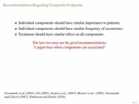
Individual components should have similar importance to patients;Individual components should have similar frequency of occurrence.Treatment should have similar effect on all components.
The last two may not be good recommendations:Largest bias when components are associated!
Data from all components should be collected until the end of trial.Individual components should be analyzed separately as the secondaryendpoints.
Allow multivariate analysis and facilitate interpretation.
46 / 53
Freemantle et al, (2003), Chi (2005), Neaton et al., (2005), Montori et al., (2005), Freemantleand Calvert (2007), Tomlinson and Detsky (2010).
Recommendations Regarding Composite Endpoints
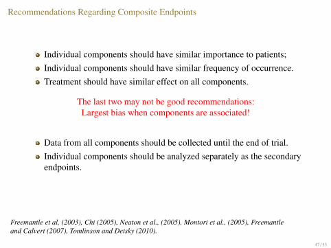
Individual components should have similar importance to patients;Individual components should have similar frequency of occurrence.Treatment should have similar effect on all components.
The last two may not be good recommendations:Largest bias when components are associated!
Data from all components should be collected until the end of trial.Individual components should be analyzed separately as the secondaryendpoints.
Allow multivariate analysis and facilitate interpretation.
47 / 53
Freemantle et al, (2003), Chi (2005), Neaton et al., (2005), Montori et al., (2005), Freemantleand Calvert (2007), Tomlinson and Detsky (2010).
Recommendations Regarding Composite Endpoints
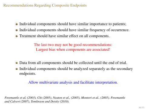
Individual components should have similar importance to patients;Individual components should have similar frequency of occurrence.Treatment should have similar effect on all components.
The last two may not be good recommendations:Largest bias when components are associated!
Data from all components should be collected until the end of trial.Individual components should be analyzed separately as the secondaryendpoints.
Allow multivariate analysis and facilitate interpretation.
48 / 53
Freemantle et al, (2003), Chi (2005), Neaton et al., (2005), Montori et al., (2005), Freemantleand Calvert (2007), Tomlinson and Detsky (2010).
Discussion
Cox model for analysis of CEP may not be appropriate: PH does nothold generally.
Many factors jointly affect the treatment effect estimation:the dependence structure in the individual components;stochastic ordering and occurrence frequencies of individual components;the amount of random censoring;heterogeneity of the treatment effect across the individual components.
“Equal treatment effect and equal frequency” of individual componentmay not be valid recommendation.
The multivariate approach generally outperforms the CEP:provides the average effect of treatment—facilitates the interpretation;can achieve higher power and accuracy;can claim treatment effect on individual components—permitintent-to-treat analysis.
49 / 53

Acknowledgment
CANNeCTIN Graduate Student Award;NSERC Postgraduate Scholarship (PGS);Ontario Graduate Scholarship (OGS).
50 / 53

ReferenceBethel MA et al. (2008) Determining the most appropriate components for a composite clinical trial outcome.
American Heart Journal doi:10.1016/j.ahj.2008.05.018.
Buzney EA, Kimball AB. (2008) A critical assessment of composite and coprimary endpoints: a complex problem.J Am Acad Dermatol 59:890-6.
Braunwald E, Cannon CP, McCabe CH, (1992) An approach to evaluating thrombolytic therapy in acutemyocardial infarction. The ‘unstatisfactory outcome’ end point. Circulation 86:683-687.
Braunwald E, Cannon CP, McCabe CH. (1993) Use of composite endpoints in thrombolysis trials of acutemyocardial infarction The American Journal of Cardiology 72 (19), pg. G3-G12
Cannon CP (1997) Clinical perspectives on the use of composite endpoints. Controlled clinical trials 18:517-529.
Chi GYH (2005) Some issues with composite endpoints in clinical trials. Fundamental & Clinical Pharmacology19:609-619.
Cook, R.J. and Lawless, J.F. (2007). The Statistical Analysis of Recurrent Events. Springer, New York.
Cox DR (1972) Regression models with lifetables (with discussion). J Roy Stat Soc Ser B 34, 187-220
Ferreira-Gonzalez et al. (2007) Problems with use of composite end points in cardiovascular trials:systematicreview of randomised controlled trials. BMJ doi:10.1136
Ferreira-Gonzalez I, Permanyer-Miralda G, Busse JW, Bryant DM, Montori VM, Alonso-Coello P, et al. (2007)Methodologic discussions for using and interpreting composite endpoints are limited, but still identify majorconcerns.J Clin Epidemiol 60:651e7.
Ferreira-Gonzalez et al. (2007) Composite endpoints in clinical trials: the trees and the forest. J Clin Epidemiol60:660-661.
Ferreira-Gonzalez et al. (2008) Composite enpoints in clinical trials. Rev Esp Cardiol 61(3):283-90.
Freemantle N et al. (2003) Composite outcomes in randomized trials: greater precision but with greateruncertainty? JAMA Vol 289. No.19 2545-2575.t
Freemantle N, Calvert M. (2007) Weighing the pros and cons for composite outcomes in clinical trials. Journal ofClinical Epidemiology 60:658-659
51 / 53
Reference
Lim Eet al. (2008) Composite outcomes in cardiovascular research: a survey of randomized trials. Ann ofIntern Med 149:612-617.
Montori VM, et al., (2005) Validity of composite end points in clinical trials. BMJ Vol 330 2005.
Neaton JD, Gray G, Zuckerman BD, Konstam M, (2005) Key issues in end point selection for heart failuretrials: composite end points. Journal of Cardiac Failure Vol.11 No. 8 2005.RTG
Prentice, RL. and Cai J. (1992) Covariance and survivor function estimation using censored multivariatefailure time data. Biometrika 79, 3:495-512.
Struthers CA and Kalbfleish JD (1986) Misspecified Proportional Hazard Models. Biometrika, 73, 363-369.
Wei, LJ, Lin,DY, and Weissfeld L. (1989) Regression Analysis of Multivariate Incomplete Failure Time Databy Modeling Marginal Distributions. Journal of American Statistical Association Vol. 84 1065-1073.
White H. (1982) Maximum Likelihood Estimation of Misspecified Models. Econometrica Vol 30:1-25.
Yusuf, et al. (2000) Effects of An Angiotensin-Converting-Enzyme Inhibitor, Ramipril, on CardiovascularEvents in High-Risk Patients. The New England Journal of Medicine Vol 342 No. 3 145-153.
52 / 53

Thank you!
53 / 53


![BLINDED EVALUATIONS OF EFFECT SIZES IN CLINICAL TRIALS ... 2013 Turkoz.pdf · endpoints in addition to sample size re-estimation • Blinded treatment effects for survival endpoints[7]](https://img.pdfslide.us/doc/110x75/608545b9f250640ece537beb/blinded-evaluations-of-effect-sizes-in-clinical-trials-2013-turkozpdf-endpoints.jpg)