Statistical Evidence Evaluation

Thomas Bayes, Pierre Simon de Laplace, Emile Zola, Sir Arthur Conan Doyle, Edmond Locard, Paul Kirk, Irving Good, Dennis Lindley

Course responsible and tutor: Anders Nordgaard (Anders.Nordgaard@liu.se)

Course web page: www.ida.liu.se/~732A45

Teaching: Lectures on theory Practical exercises (mostly with software) Discussion of assignments

Course book: Taroni F., Aitken C., Garbolino P., Biedermann A., Bayesian

Networks and Probabilistic Inference in Forensic Science, Chichester: Wiley, 2006

A course on probabilistic reasoning, graphical modelling and applications on evaluation of forensic evidence and decision making

Additional literature: Taroni F., Bozza S., Biedermann A., Garbolino P., Aitken C.

Data analysis in forensic science, Chichester: Wiley, 2010. Scientific papers (will be announced later)

Software: GeNIe Download at http://genie.sis.pitt.edu/

Examination: Assignments (compulsory to pass) Final oral exam (compulsory, decides the grade)

Today: Repeat and extend…

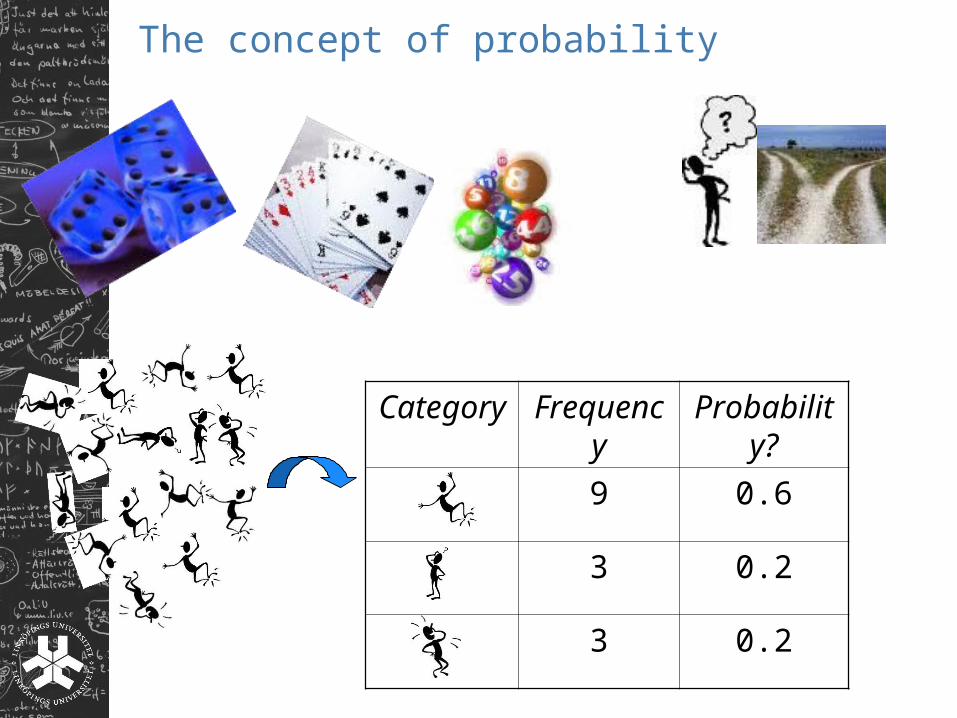
The concept of probability

Category Frequency Probability?

9 0.6

3 0.2

3 0.2

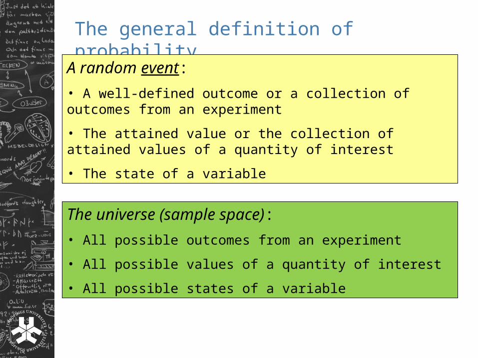
The general definition of probability

A random event:

• A well-defined outcome or a collection of outcomes from an experiment

• The attained value or the collection of attained values of a quantity of interest

• The state of a variable

The universe (sample space):

• All possible outcomes from an experiment

• All possible values of a quantity of interest

• All possible states of a variable

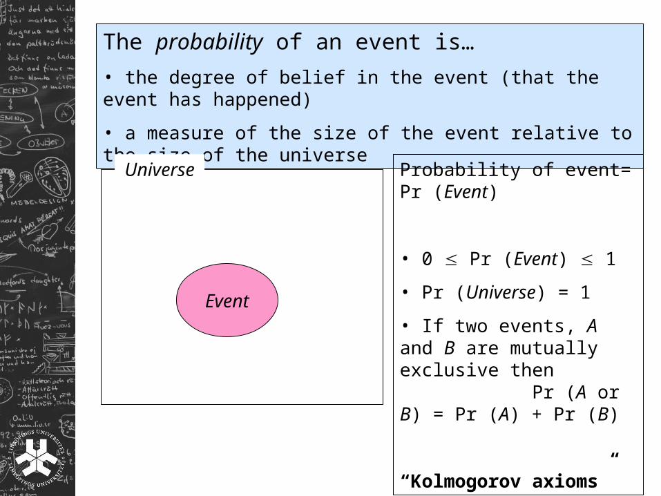
The probability of an event is…

• the degree of belief in the event (that the event has happened)

• a measure of the size of the event relative to the size of the universe

Universe

Event

Probability of event= Pr (Event)

• 0 Pr (Event) 1

• Pr (Universe) = 1

• If two events, A and B are mutually exclusive then Pr (A or B) = Pr (A) + Pr (B)

“Kolmogorov axioms”

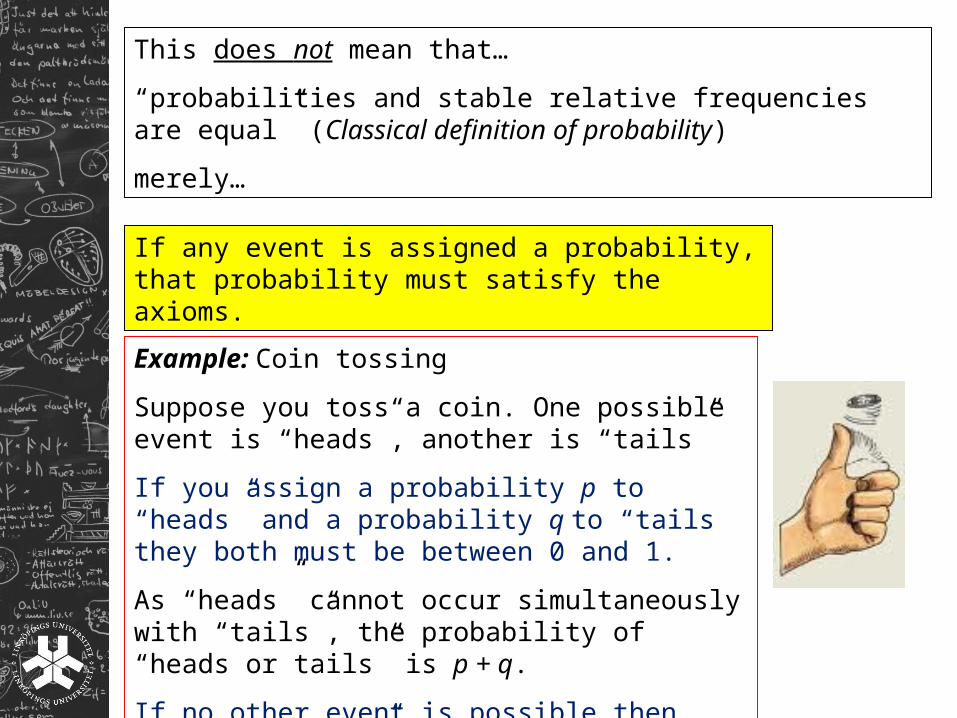
This does not mean that…

“probabilities and stable relative frequencies are equal” (Classical definition of probability)

merely…

If any event is assigned a probability, that probability must satisfy the axioms.

Example: Coin tossing

Suppose you toss a coin. One possible event is “heads”, another is “tails”

If you assign a probability p to “heads” and a probability q to “tails they both must be between 0 and 1.

As “heads” cannot occur simultaneously with “tails”, the probability of “heads or tails” is p + q.

If no other event is possible then “heads or tails” = Universe p + q = 1

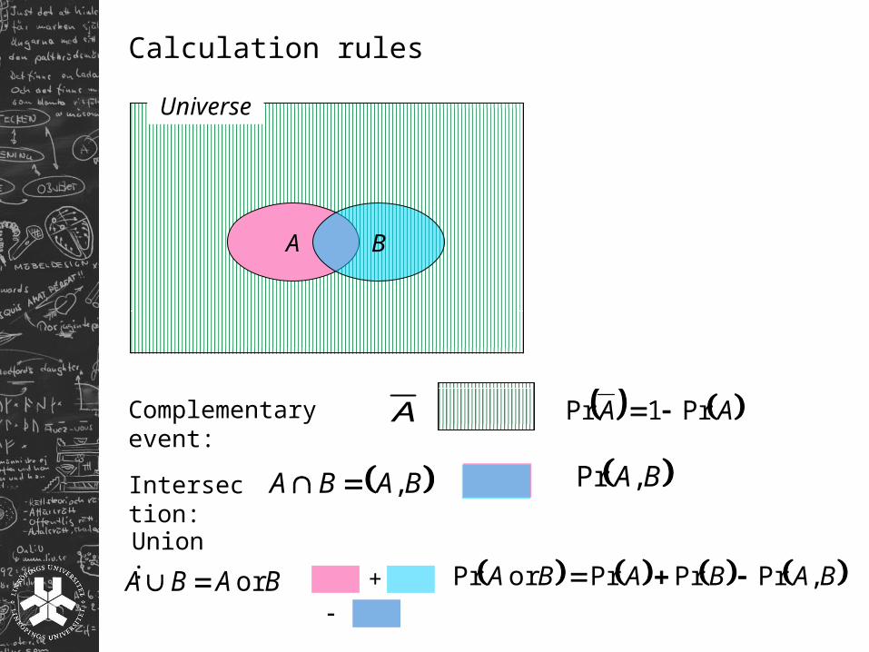
Calculation rules

Universe

A B

Complementary event: A AA Pr1Pr

Union:

Intersection: BABA , BA,Pr

BABA or + BABABA ,PrPrPror Pr

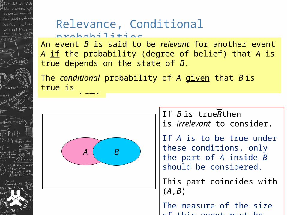
If B is true then is irrelevant to consider.

If A is to be true under these conditions, only the part of A inside B should be considered.

This part coincides with (A,B)

The measure of the size of this event must be relative to the size of B

Relevance, Conditional probabilities

B

BABA

Pr

,PrPr

B

An event B is said to be relevant for another event A if the probability (degree of belief) that A is true depends on the state of B.

The conditional probability of A given that B is true is

A B

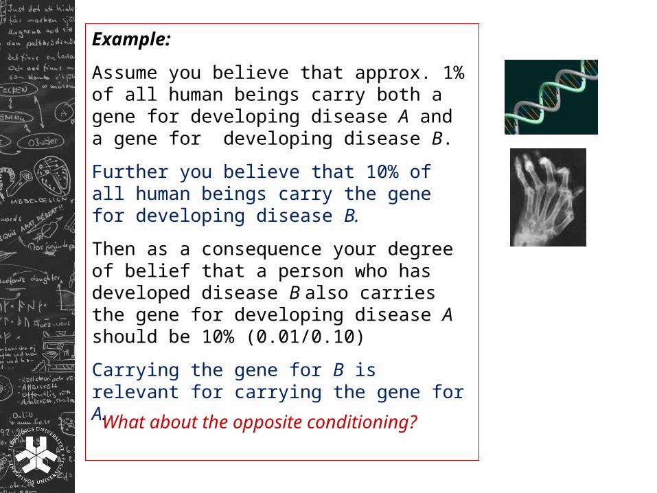
Example:

Assume you believe that approx. 1% of all human beings carry both a gene for developing disease A and a gene for developing disease B.

Further you believe that 10% of all human beings carry the gene for developing disease B.

Then as a consequence your degree of belief that a person who has developed disease B also carries the gene for developing disease A should be 10% (0.01/0.10)

Carrying the gene for B is relevant for carrying the gene for A.

What about the opposite conditioning?

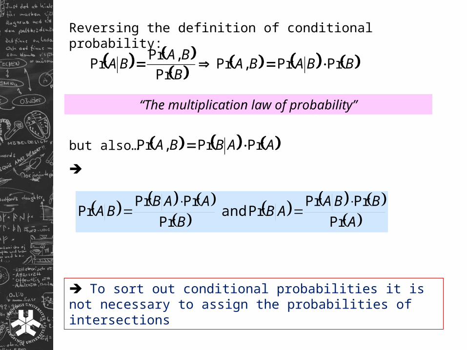
Reversing the definition of conditional probability:

BBABAB

BABA PrPr,Pr

Pr

,PrPr

“The multiplication law of probability”

but also…

AABBA PrPr,Pr

A

BBAAB

B

AABBA

Pr

PrPrPr and

Pr

PrPrPr

To sort out conditional probabilities it is not necessary to assign the probabilities of intersections

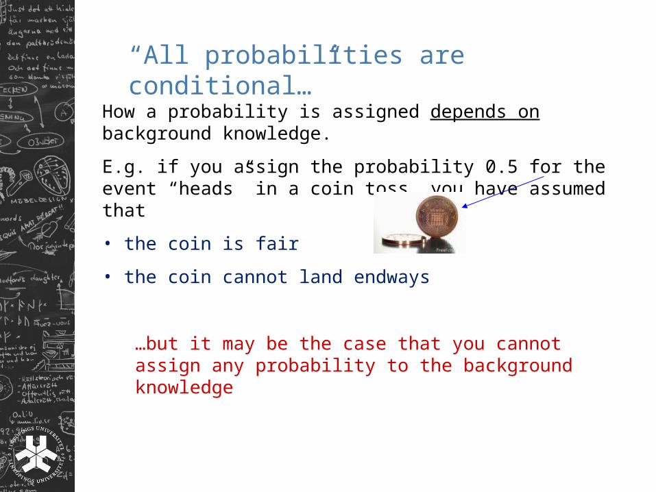
“All probabilities are conditional…”

How a probability is assigned depends on background knowledge.

E.g. if you assign the probability 0.5 for the event “heads” in a coin toss, you have assumed that

• the coin is fair

• the coin cannot land endways

…but it may be the case that you cannot assign any probability to the background knowledge

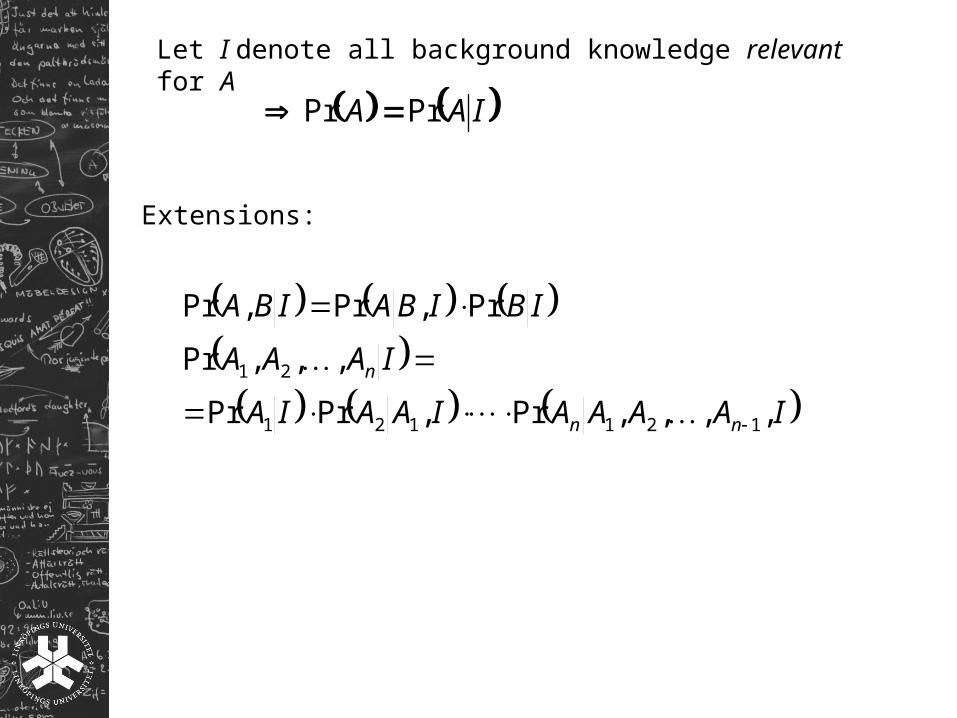
Let I denote all background knowledge relevant for A

IAA PrPr

Extensions:

IAAAAIAAIA

IAAA

IBIBAIBA

nn

n

,,,,Pr,PrPr

,,,Pr

Pr,Pr,Pr

121121

21

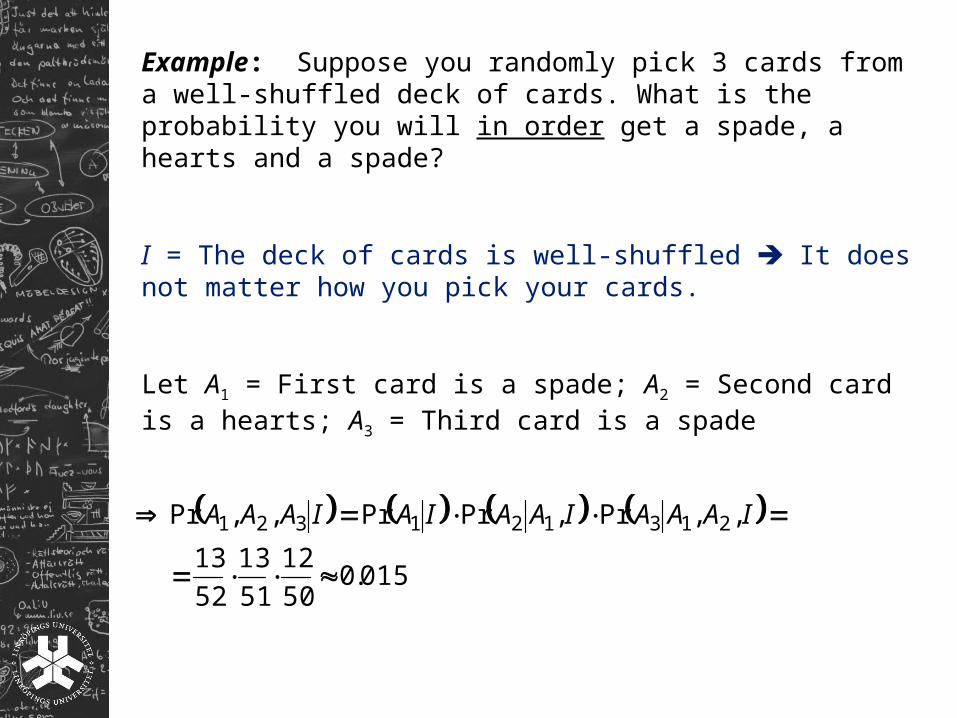
Example: Suppose you randomly pick 3 cards from a well-shuffled deck of cards. What is the probability you will in order get a spade, a hearts and a spade?

I = The deck of cards is well-shuffled It does not matter how you pick your cards.

Let A1 = First card is a spade; A2 = Second card is a hearts; A3 = Third card is a spade

015.0

50

12

51

13

52

13

,,Pr,PrPr,,Pr 213121321

IAAAIAAIAIAAA

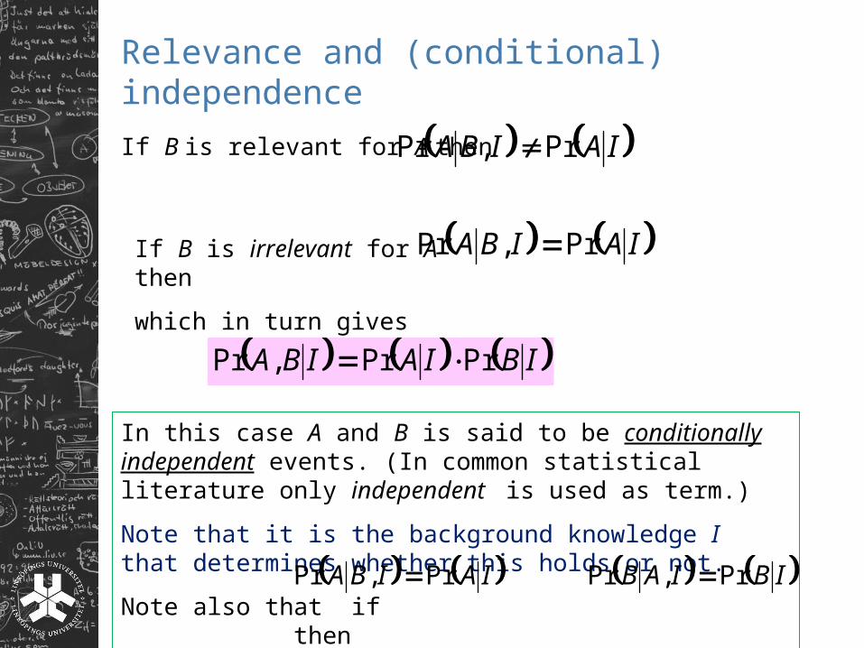
Relevance and (conditional) independence

IAIBA Pr,Pr If B is relevant for A then

If B is irrelevant for A then

which in turn gives

IAIBA Pr,Pr

IBIAIBA PrPr,Pr

In this case A and B is said to be conditionally independent events. (In common statistical literature only independent is used as term.)

Note that it is the background knowledge I that determines whether this holds or not.

Note also that if then

Irrelevance is reversible!

IAIBA Pr,Pr IBIAB Pr,Pr

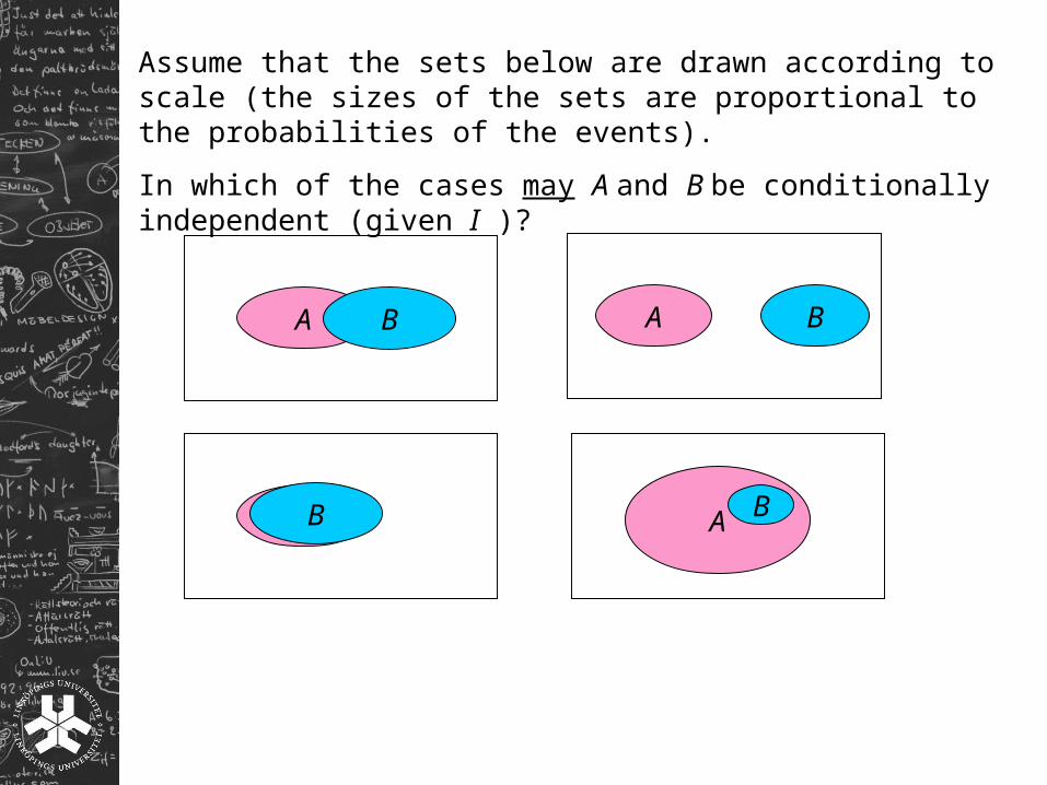
Assume that the sets below are drawn according to scale (the sizes of the sets are proportional to the probabilities of the events).

In which of the cases may A and B be conditionally independent (given I )?

A B

AB A B

A B

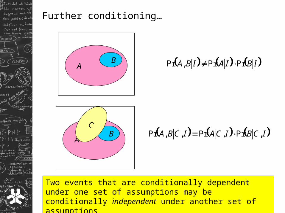
Further conditioning…

AB IBIAIBA PrPr,Pr

AB

C

ICBICAICBA ,Pr,Pr,,Pr

Two events that are conditionally dependent under one set of assumptions may be conditionally independent under another set of assumptions

The law of total probability and Bayes’ theorem

A B IBIBAIBIBA

IBAIBAIA

Pr,PrPr,Pr

,Pr,PrPr

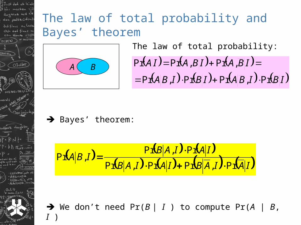
The law of total probability:

Bayes’ theorem:

IAIABIAIAB

IAIABIBA

Pr,PrPr,Pr

Pr,Pr,Pr

We don’t need Pr(B | I ) to compute Pr(A | B, I )

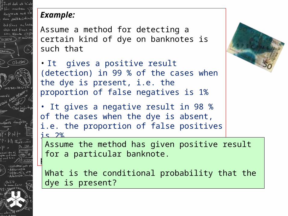
Example:

Assume a method for detecting a certain kind of dye on banknotes is such that

• It gives a positive result (detection) in 99 % of the cases when the dye is present, i.e. the proportion of false negatives is 1%

• It gives a negative result in 98 % of the cases when the dye is absent, i.e. the proportion of false positives is 2%.

The presence of dye is rare: prevalence is about 0.1 %

Assume the method has given positive result for a particular banknote.

What is the conditional probability that the dye is present?

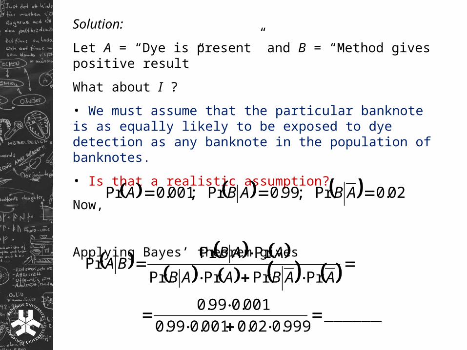
Solution:

Let A = “Dye is present” and B = “Method gives positive result”

What about I ?

• We must assume that the particular banknote is as equally likely to be exposed to dye detection as any banknote in the population of banknotes.

• Is that a realistic assumption?

Now,

Applying Bayes’ theorem gives

02.0Pr;99.0Pr;001.0Pr ABABA

_______999.002.0001.099.0

001.099.0

PrPrPrPr

PrPrPr

AABAAB

AABBA

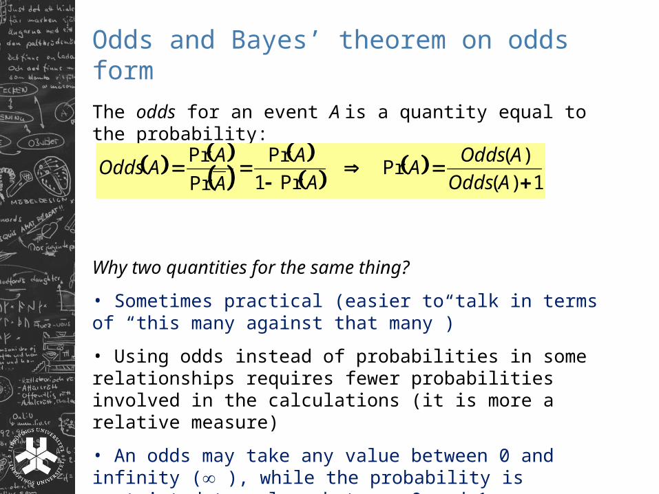
Odds and Bayes’ theorem on odds form

The odds for an event A is a quantity equal to the probability:

Why two quantities for the same thing?

• Sometimes practical (easier to talk in terms of “this many against that many”)

• Using odds instead of probabilities in some relationships requires fewer probabilities involved in the calculations (it is more a relative measure)

• An odds may take any value between 0 and infinity ( ), while the probability is restricted to values between 0 and 1.

1)(

)(Pr

Pr1

Pr

Pr

Pr

AOdds

AOddsA

A

A

A

AAOdds

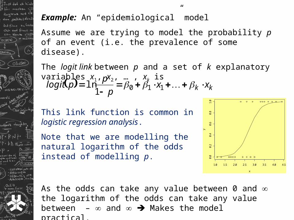
Example: An “epidemiological” model

Assume we are trying to model the probability p of an event (i.e. the prevalence of some disease).

The logit link between p and a set of k explanatory variables x1, x2, … , xk is

kk xxp

pplogit

1101

ln

This link function is common in logistic regression analysis.

Note that we are modelling the natural logarithm of the odds instead of modelling p.

1.0 1.5 2.0 2.5 3.0 3.5 4.0 4.5

0.0

0.2

0.4

0.6

0.8

1.0

x

y

As the odds can take any value between 0 and the logarithm of the odds can take any value between – and Makes the model practical.

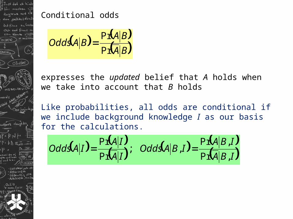
Conditional odds

BA

BABAOdds

Pr

Pr

Like probabilities, all odds are conditional if we include background knowledge I as our basis for the calculations.

IBA

IBAIBAOdds

IA

IAIAOdds

,Pr

,Pr,;

Pr

Pr

expresses the updated belief that A holds when we take into account that B holds

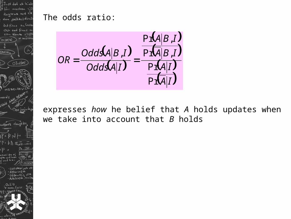
The odds ratio:

IA

IA

IBA

IBA

IAOdds

IBAOddsOR

Pr

Pr

,Pr

,Pr

,

expresses how he belief that A holds updates when we take into account that B holds

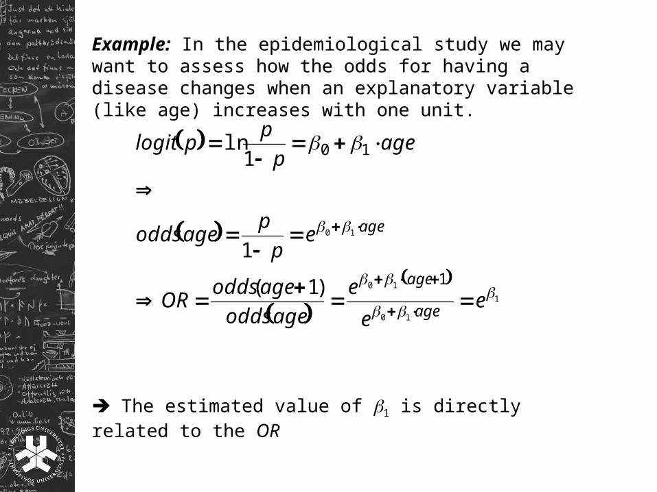
Example: In the epidemiological study we may want to assess how the odds for having a disease changes when an explanatory variable (like age) increases with one unit.

1

10

10

10

1

10

)1(

1

1ln

ee

e

ageodds

ageoddsOR

ep

pageodds

agep

pplogit

age

age

age

The estimated value of 1 is directly related to the OR

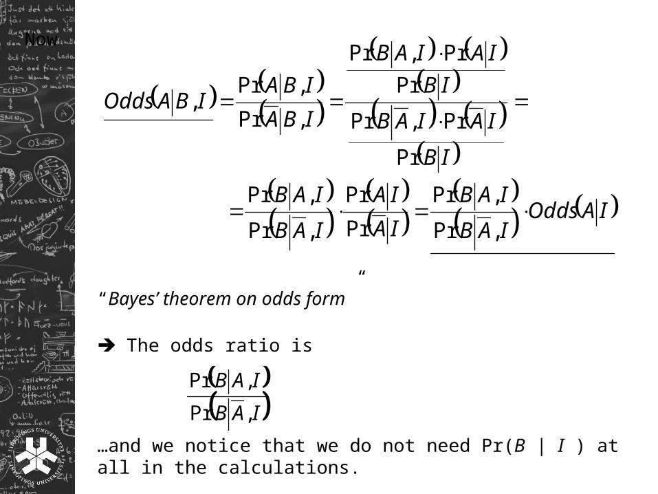
Now

IAOdds

IAB

IAB

IA

IA

IAB

IAB

IB

IAIAB

IB

IAIAB

IBA

IBAIBAOdds

,Pr

,Pr

Pr

Pr

,Pr

,Pr

Pr

Pr,Pr

Pr

Pr,Pr

,Pr

,Pr,

The odds ratio is

…and we notice that we do not need Pr(B | I ) at all in the calculations.

IAB

IAB

,Pr

,Pr

“Bayes’ theorem on odds form”

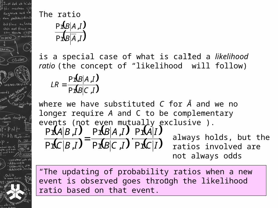
The ratio

is a special case of what is called a likelihood ratio (the concept of “likelihood” will follow)

IAB

IAB

,Pr

,Pr

ICB

IABLR

,Pr

,Pr

where we have substituted C for Ā and we no longer require A and C to be complementary events (not even mutually exclusive ).

IC

IA

ICB

IAB

IBC

IBA

Pr

Pr

,Pr

,Pr

,Pr

,Pr always holds, but the ratios

involved are not always odds

“The updating of probability ratios when a new event is observed goes through the likelihood ratio based on that event.”

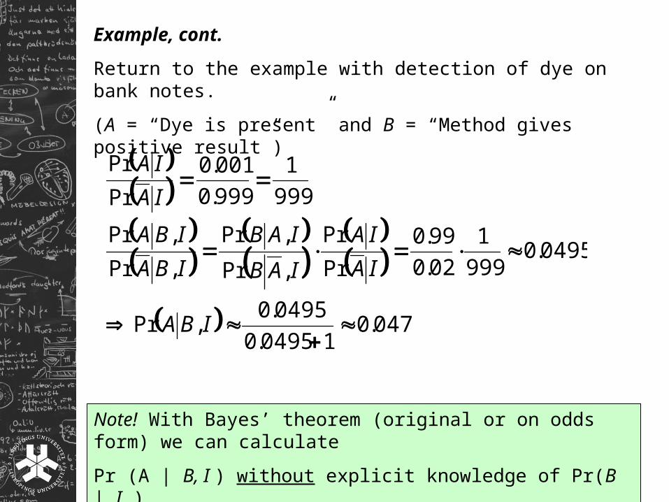
Example, cont.

Return to the example with detection of dye on bank notes.

(A = “Dye is present” and B = “Method gives positive result”)

047.010495.0

0495.0,Pr

0495.0999

1

02.0

99.0

Pr

Pr

,Pr

,Pr

,Pr

,Pr

999

1

999.0

001.0

Pr

Pr

IBA

IA

IA

IAB

IAB

IBA

IBA

IA

IA

Note! With Bayes’ theorem (original or on odds form) we can calculate

Pr (A | B, I ) without explicit knowledge of Pr(B | I )

Random variables and parameters

For physical measurements but also for observations it is most often convenient to formalise an event as a (set of) outcome(s) of a variable.

A random variable is a variable, the value of which is not known in advance and cannot be exactly forecasted.

All variables of interest in a measurement situation would be random variables.

A parameter is another kind of variable, that is assumed to have a fixed value throughout the experiment (scenario, survey).

A parameter can often be controlled and its value is then known in advance (i.e. can be exactly forecasted)

The value attained by a random variable is usually called state

Examples:

1) Inventory of a grassland.

One random variable can be the are percentage covered by a specific weed.

The states of this variable constitute the range from zero to the total area of the grassland

One parameter can be the distance from the grassland to the nearest water course.

2) DNA profiling

One random variable can be the genotype in a locus of the DNA double helix (genotype = the combination of two alleles, one inherited from the mother and one from the father; DNA double helix = the “entire DNA”)

The states of this variable are all possible combinations of alleles in that locus.

One parameter can be the locus itself