Statistical and Low Temperature Physics (PHYS393) - University of

Statistical and Low Temperature Physics(PHYS393)

Kai Hock

2011 - 2012

University of Liverpool

Recommended reading:

1. Statistical Mechanics - A Survival Guide,

A. M. Glazer and J. S. Wark

Oxford University Press, 2001

2. Basic Superfluids

Tony Guenault

Taylor & Francis Inc., 2003

Both available as ebooks in the Liverpool University library.

Basic Statistical Mechanics 1

Required Background

Required Background

1. Thermodynamics (PHYS253)

(Covers most of the basic ideas. It would help to look

through the notes again.)

2. Quantum and Atomic Physics (PHYS255)

(You need: Schrodinger’s equation, particle in a box, simple

harmonic oscillator, Zeeman effect, fermions and bosons.)


CONTENTS

Part 1: Statistical Mechanics

1. Basic statistical mechanics.

2. Electrons in metals.

3. Photons and phonons.

4. Application to cooling techniques.

Part 2: Superfluids and Superconductors

5. Matter at Low Temperatures.

6. Liquid Helium-4.

7. Superconductivity.

8. Liquid Helium-3.


Statistical and Low Temperature Physics (PHYS393)

1. Basic Statistical Mechanics

Kai Hock

2011 - 2012

University of Liverpool


A brief review

1. Thermodynamics

2. Quantum mechanics

3. Statistical mechanics

4. Paramagnetic salts

5. Ideal gas


Thermodynamics, briefly.


Heat capacities

This graph shows the heat capacity of copper. At high

temperatures (T ), it tends to a constant. At low T , it falls to

zero.

The main theme in Part 1 is to learn how to explain such

behaviours.Basic Statistical Mechanics 7

Entropy

The study of heat engines in the 19th century led Rudolf

Clausius to propose in 1982 the second law of thermodynamics

in this form: “In a closed cycle, the sum of δQ/T is zero.”

http://en.wikipedia.org/wiki/Entropy

δQ is an infinetesimal heat change. Later, δQ/T came to be

written as δS, or

dQ = TdS,

and S became known as the entropy.

Clausius statement implies that this abstract quantity S is a

state function. E.g. if you compress and expand a gas and go

back to the initial p and V at the end, then S also returns to

the same value. (Note that Q itself is not a state function.)


Chemical potential.

The chemical potential µ is equal to the Gibbs free energy at

equilibrium. The Gibbs free energy is

G = U + pV − TS.

One simple use of µ is to find the energy change between two

phases at constant p and T :

∆µ = ∆U + p∆V − T∆S.

At phase transition between liquid and gas, this would be the

energy difference between 1 mole of liquid changing to gas, and

1 mole of gas changing to liquid at the same T and p. So

∆µ = 0

gives the condition for phase equilibrium, because then there is

no energy advantage in more liquid changing to gas, or the

other way round.

http://en.wikipedia.org/wiki/Gibbs_free_energy


Quantum mechanics, briefly.


Schrodinger’s equation.

This is the 1D Schrodinger’s equation.

~2

2m

dψ

dx+ V (x)ψ = Eψ,

where m is the mass of a particle, ψ is the wavefunction, V (x)

the potential it experiences, and E its energy.

In free space, V (x) would be zero. Solving the equation then

gives

ψ = eikx or e−ikx,

where k is related to E given by

E =~2k2

2m.


Momentum.

The Schrodinger’s equation is based on the postulate for the

momentum px of a particle:

−i~ ddx

= px.

We use this on a wavefunction ψ like this:

−i~dψdx

= pxψ.

Applying this to the free space wavefunction eikx, we find

px = ~k.


Particle in a box

In a 1D box of length L, the potential V (x) could be zero for x

between 0 and L, and infinity otherwise.

This means that the wavefunction must be zero outside the

box, and also zero at the “walls” at x equals 0 and L.

Inside the box, it is like free space, so ψ is eikx or e−ikx. In order

for ψ to be zero at the walls, these can be combined to give

ψ = sin kx =eikx − e−ikx

2i.

Applying the condition that this is zero at the walls, we find

k =nπ

L,

where n is an integer. This shows that the energy is quantised:

E =~2k2

2m=n2π2~2

2mL2.


Statistical mechanics


Microstates

In quantum mechanics, energies are often quantised. We have

seen that this happens for a particle in a box.

Consider a system with N particles. This could be atoms in a

solid. For now, think of each one like a particle in a box.

Suppose every particle has energy levels ε1, ε2, ...

A microstate refers to a specific arrangement of particles

among the energy levels, e.g. particle 1 in ε3, particle 2 in ε1, ...

A macrostate refers to a distribution of particles among the

levels, e.g. 6 particles are in ε1, 4 particles are in ε2, ...


Macrostate.

Suppose there are n1 particles in ε1, n2 particles in ε2, ...

The macrostate can be written as (n1, n2, ...), or simply niwhere i = 1, 2, ... Then

N = n1 + n2 + ...

Suppose the system is thermally isolated from the surrounding,

so that the total energy E is constant. E is given by

E = n1ε1 + n2ε2 + ...

These two equations impose constraints on the number of

particles possible on each energy level.


Postulate of equal a priori probabilities

More than one microstate can have the same macrostate. E.g.

if the macrostate has 4 particles are in ε2, then these 4

particles can be any of the N particles.

Basic postulate of statistical mechanics:

“A system is equally likely to be in any microstate that satisfies

the constraints.”

This means that a system is most likely be be in the

macrostate with the largest number of microstates. We may

call this the most probably macrostate.

Using the method of statistics, it can be shown that if N is

very large, then the probability of other macrostates is very

close to zero. (E.g. when you take the average of more

readings in an experiement, the error gets smaller.)


Constraints

Assuming the constraints

N = n1 + n2 + ...

and

U = n1ε1 + n2ε2 + ...

it is possible to solve for the most probably macrostate usingthe method of Lagrange multipliers.

Before that, we need to write down the number of possiblemicrostates for a the macrostate. This is just the number ofways to arrange N different objects in some boxes, with n1objects in box (level) 1, n2 objects in box 2, and so on.

Using the method of combinations, the number ofarrangements is

Ω =N !

n1!n2!...

The problem is to find the values of ni that gives the largest Ω.


Method of Lagrange multipliers.

The steps are as follows.

1. Write down the Lagrange function ln Ω + λ1N + λ2U .Two new variables, λ1 and λ2, have to be introduced.

2. Differentiate with respect to each of ni and λ1, λ2.

3. Set all derivatives to zero. Solve the equations for ni.

The answer is:

ni = A exp(λ2εi)

where A is exp(λ1).

There are two unknowns A and λ2. In principle, we cansubstitute into the above constraints and solve for these.Unfortunately, the equations are too complicated.


Boltzmann’s postulate

Around 1872, Ludwig Boltzmann postulated the connection

between entropy S and the number of macrostates Ω:

S = kB ln Ω.

This formula allows us to use thermodynamics, e.g. using

dQ = TdS,

to find the answer to the most probable macrostate. Assuming

Boltzmann’s postulate, it can be shown that

λ2 = −1/kBT,

so that the distribution becomes

ni = A exp(−εi/kBT ).

This is now called the Boltzmann distribution.


Paramagnetic salts


Paramagnetic salts.

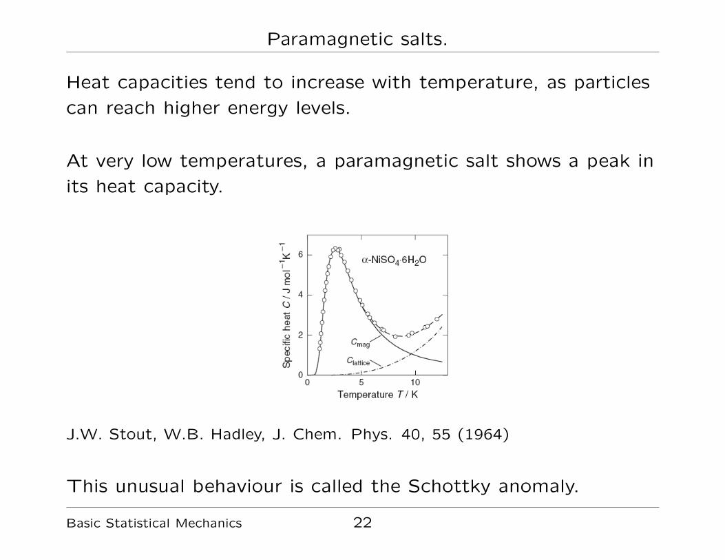
Heat capacities tend to increase with temperature, as particles

can reach higher energy levels.

At very low temperatures, a paramagnetic salt shows a peak in

its heat capacity.

J.W. Stout, W.B. Hadley, J. Chem. Phys. 40, 55 (1964)

This unusual behaviour is called the Schottky anomaly.


Schottky anomaly

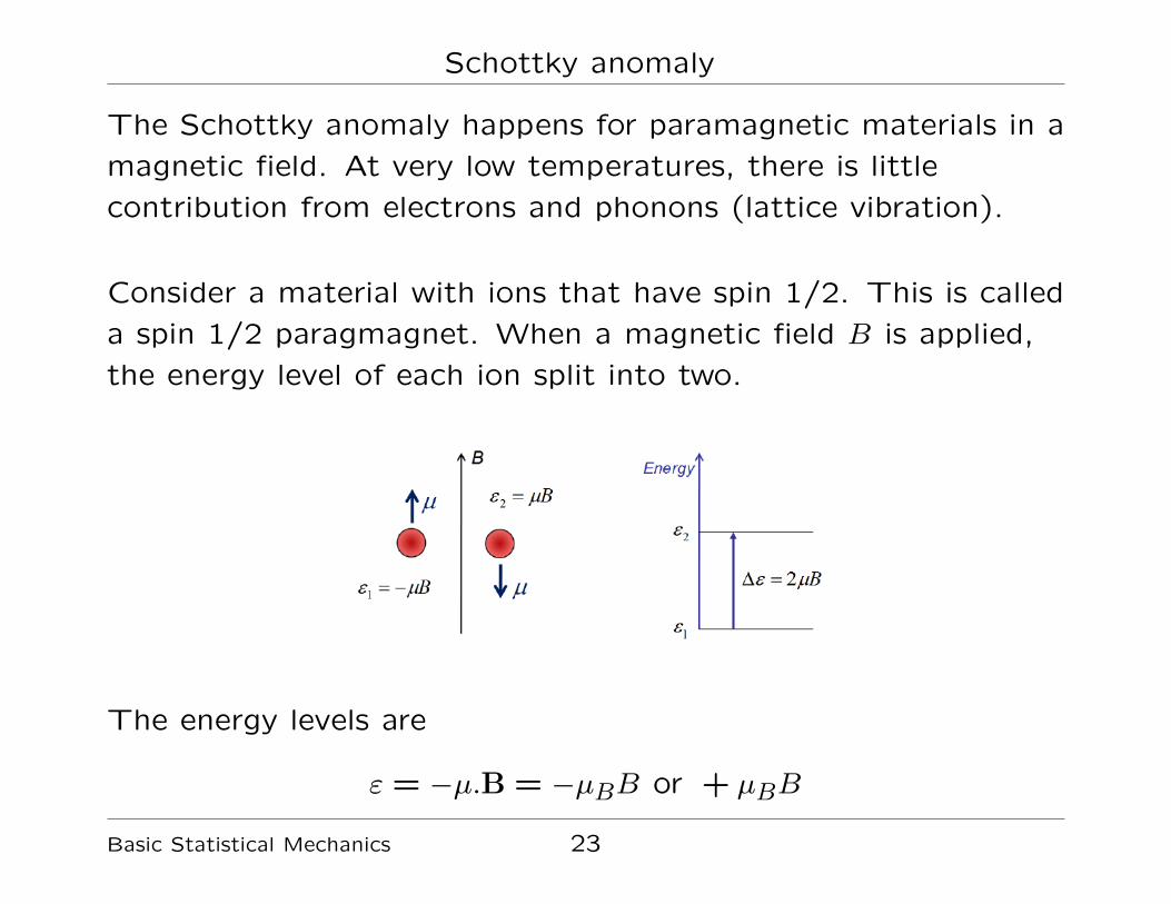
The Schottky anomaly happens for paramagnetic materials in a

magnetic field. At very low temperatures, there is little

contribution from electrons and phonons (lattice vibration).

Consider a material with ions that have spin 1/2. This is called

a spin 1/2 paragmagnet. When a magnetic field B is applied,

the energy level of each ion split into two.

The energy levels are

ε = −µ.B = −µBB or + µBB


Lets see if we can “deduce” the Schottky anomally. At 0 K, all

electrons are at the ground state, so the total energy U is

−NµBB, where N is the number of the ions.

At high temperatures, the thermal energy the electrons is much

larger than the difference between the two magnetic energy

levels. Then the electrons are equally likely to be in −µBB or

+µBB, so U is zero

A sketch of U against T would look like this.


Heat capacity

In principle, we can now find the heat capacity C using

C =dU

dT.

However, the gradient of U neat 0 K is not known. We can find

this using the Boltzmann distribution.

Near 0 K, nearly all electrons at at the lower state. The very

small fraction in the higher state is approximately given by the

Boltzmann factor exp(−ε/kBT ) (why?), where

ε = 2µBB.

The total energy is then

U = −NµBB +NµBB exp(−ε/kBT ).

Differentiating this shows that the gradient goes to zero as T

goes to 0 K.


Now that we know the gradient is zero at both 0 K and high T

we can sketch the heat capacity, which is the gradient of U .

We have just deduced the Schottky anomaly.


We shall now use the Boltzmann distribution to derive aformula for U and C. There are two levels:

ε1 = −µBB and ε2 = +µBB.

The total energy is

U =∑

niεi

The number of electrons in level i is given by

ni = A exp(−εi/kBT ).

We must solve for A first. The total number is

N = A∑

exp(−εi/kBT ).

The sum is called the single particle partition function:

ZSP =∑

exp(−εi/kBT )

Solving for A gives

A =N

ZSP.


So

ni =N

ZSPexp(−εi/kBT ).

The total energy is

U =∑

niεi

Substituting ni:

U =N

ZSP

∑εi exp(−εi/kBT ).

Substituting for εi:

U =N

ZSP[−µBB exp(µBB/kBT ) + µBB exp(−µBB/kBT )].

and in ZSP as well:

U = N−µBB exp(µBB/kBT ) + µBB exp(−µBB/kBT )

exp(µBB/kBT ) + exp(−µBB/kBT )

Simplifying, we find U :

U = −NµBB tanh(µBB/kBT ).


The formula

U = −NµBB tanh(µBB/kBT ).

does indeed give the graph that we deduced earlier on:

We note here that a useful formula from the above formula for

ni, is the probability that an electron is at level εi:

pi =niN

=exp(−εi/kBT )

Z.


Differentiating U gives the heat capacity:

C = NkB

(µBB

kBT

)2

sech2(µBB

kBT

).

which also gives the Schottky anomaly that we deduced:


The entropy.

We can find the entropy using

dS =dQ

T=dU

T.

In our case, Q is just U since no work is done. So

S =∫dU

T=∫CdT

T.

This can be done analytically using the earlier formula for C.

The result is

S = NkB ln

[2 cosh

(µBB

kBT

)]−NµBB

Ttanh

(µBB

kBT

).


The entropy.

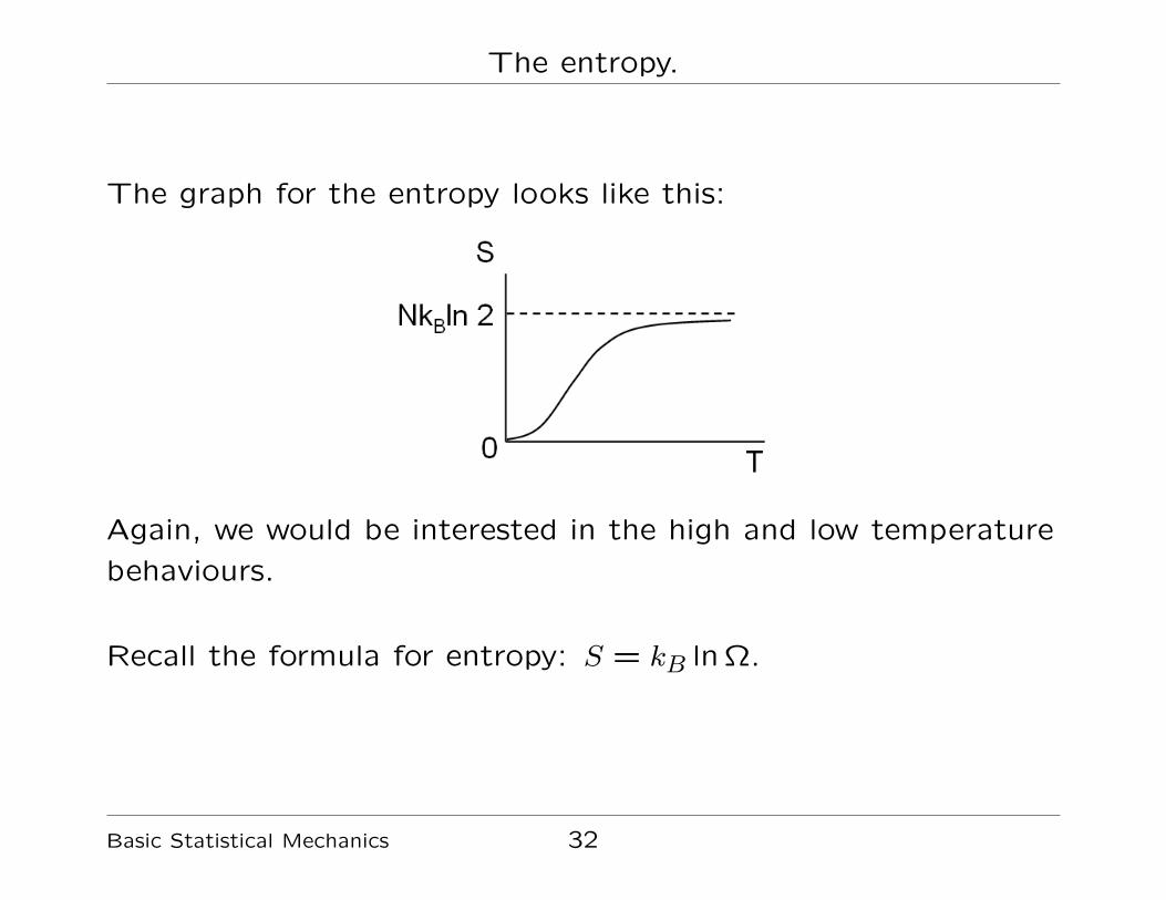
The graph for the entropy looks like this:

Again, we would be interested in the high and low temperature

behaviours.

Recall the formula for entropy: S = kB ln Ω.


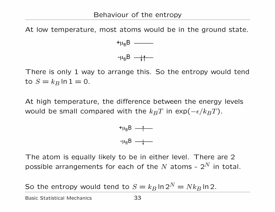
Behaviour of the entropy

At low temperature, most atoms would be in the ground state.

There is only 1 way to arrange this. So the entropy would tend

to S = kB ln 1 = 0.

At high temperature, the difference between the energy levels

would be small compared with the kBT in exp(−ε/kBT ).

The atom is equally likely to be in either level. There are 2

possible arrangements for each of the N atoms - 2N in total.

So the entropy would tend to S = kB ln 2N = NkB ln 2.


Ideal Gas


A particle in a 3-D box

In an ideal gas, we assume that there is little interaction

between atoms.

From the kinetic theory of gases, we know that the average

energy of each atom in an ideal gas is

1

2mv2 =

3

2kBT.

This means that the total energy is

U =3

2NkBT

and the heat capacity is

C =dU

dT=

3

2NkB.

http://en.wikipedia.org/wiki/Kinetic_theory

We shall rederive this here using statistical mechanics. The

ideas will also be used for electrons and phonons.


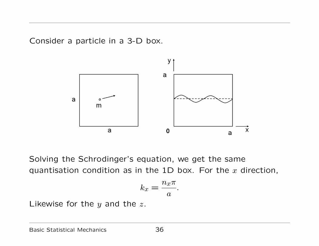
Consider a particle in a 3-D box.

Solving the Schrodinger’s equation, we get the same

quantisation condition as in the 1D box. For the x direction,

kx =nxπ

a.

Likewise for the y and the z.


Density of states.

To find the heat capacity of N particles, we need the energy

U =∑

niεi.

For the spin 1/2 salt, there are only 2 levels to sum. For the

particle in the box, there are many levels.

At room temperature, many of these levels could be occupied.

This is because for an ideal gas, spacing between energy levels

is much smaller than the average energy of a particle. (Prove

it.)

As a result, a plot of ni against εi may look like this.


Density of states.

This suggests that we may approximate the graph to a curve,and the sum to an integral.

Within a small interval dε, ni is nearly constant. Then the sumof the energies of particles is approximately niεi times thenumber of states in this interval.

If we divide this number of states by dε, we can think of thethe answer as a kind of density. This density of states (DOS) isoften denoted by the function g(εi).

The number states in dε is then g(εi)dε, and the energy in theinterval given by niεig(εi)dε.


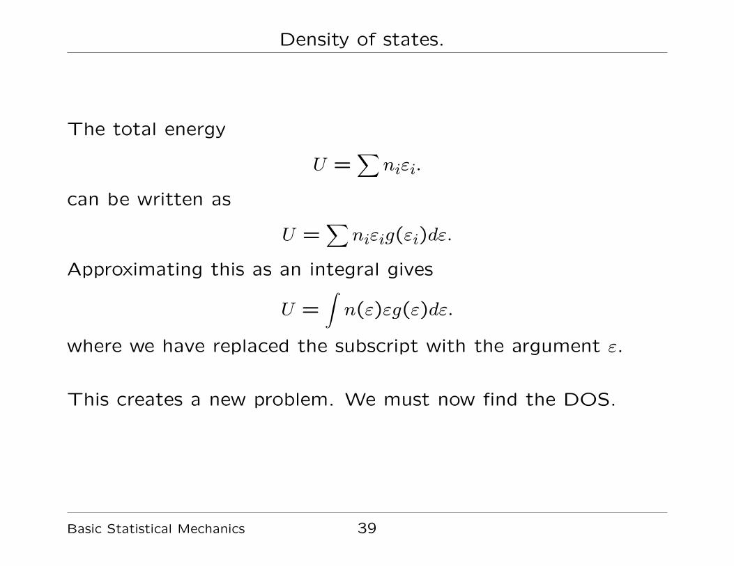
Density of states.

The total energy

U =∑

niεi.

can be written as

U =∑

niεig(εi)dε.

Approximating this as an integral gives

U =∫n(ε)εg(ε)dε.

where we have replaced the subscript with the argument ε.

This creates a new problem. We must now find the DOS.


Counting states

The wavevectors

kx =nxπ

a

are quantised at uniform intervals in all three directions.

we can imagine a k space in which the the x coordinate is kx,

and so on. If we use a point to represent each state, we would

get a lattice like this.


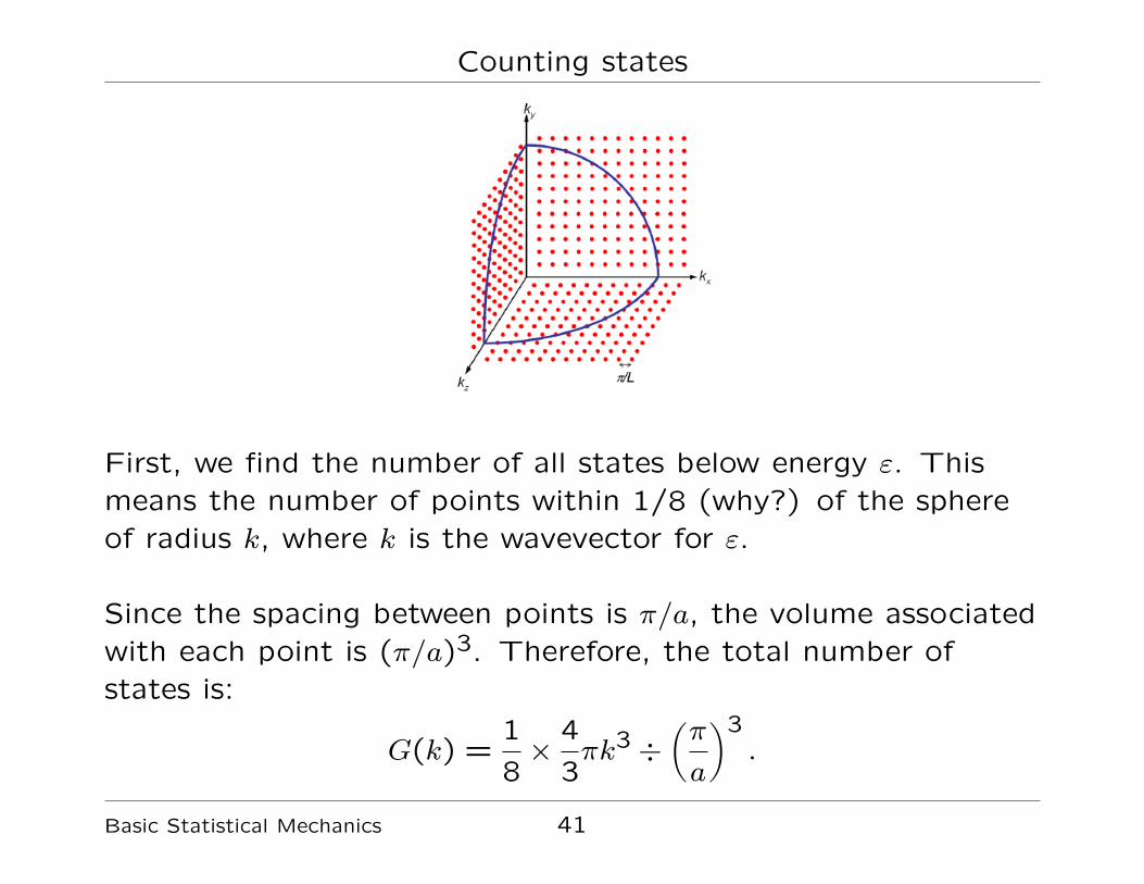
Counting states

First, we find the number of all states below energy ε. Thismeans the number of points within 1/8 (why?) of the sphereof radius k, where k is the wavevector for ε.

Since the spacing between points is π/a, the volume associatedwith each point is (π/a)3. Therefore, the total number ofstates is:

G(k) =1

8×

4

3πk3 ÷

(π

a

)3.


DOS

We find that the total number of states below k is

G(k) =V k3

6π2,

where V is the volume a3 of the box.

Suppose k is increased by dk. Then the number of states

increases by dG. So the density of states is

g(k) =dG(k)

dk=V k2

2π2.

We have earlier defined the DOS in terms of energy, g(ε).

Important: To convert the variable to energy, it is not a simple

matter of substituting the formula

ε =~2k2

2m.


Changing variables

The reason is that for the same interval ε, the size of the

interval dk can be different at different energy because the

relation

ε =~2k2

2m

is not linear. (Prove it.)

The correct way is to use the method for probability density

function:

gε(ε)dε = gk(k)dk.

http://en.wikipedia.org/wiki/Probability_density_function

The subscripts are added here to emphasise that g(ε) and g(k)

are different functions.


Changing variables

Rearranging,

gε(ε) = gk(k)dk

dε.

We can now substitute the relation

ε =~2k2

2m

to find gε(ε). The answer is

g(ε) =4mπV

h3(2mε)1/2

where we have dropped the subscript again, as is the normal

practice. (Misleading, but you can tell from the argument.)

For comparison:

g(k) =V k2

2π2.


Changing variables

It is also useful to have the formula for total number states

G(k) =1

8×

4

3πk3 ÷

(π

a

)3.

in terms of energy.

Since no ε or k intervals are involved, we can simply substitute

ε =~2k2

2m.

The answer is

G(ε) =4πV

3h3(2mε)3/2.


Ideal gas energy states

In an ideal gas at room temperature, it is very unlikely for two

or more atoms to occupy the same energy state. So we can

assume that each state is occupied by only one atom. This

simplifies the calculation of the macrostate.

First, we should justify the assumption.

At a temperature T , we know from simple kinetic theory of

ideal gas that the average energy of a gas atom is about

3kBT/2.

We need to know how many energy states there are below this

energy at room temperature.



We can use the formula we have derived:

G(ε) =4πV

3h3(2mε)3/2

by setting ε = 3kBT/2.

Putting in the numbers for one mole of ideal gas at room

temperature, we find that the number of states below 3kBT/2

is about 1030.

1 mole of gas contains about 1024 atoms.

This means we have about 1030 ÷ 1024 = 106 states per atom.



This means we have about 1 million energy states for every

atom.

So it is extremely unlikely that two atoms would ever occupy

the same energy state.

We can use this result to derive the energy distribution of these

atoms, with the help of the Lagrange multipliers.


Indistinguishable particles.

Consider a interval εi around the energy εi. Suppose there are

are ni atoms and gi states in this interval.

We need to find the number of microstates. We cannot do it

the same way as in the paramagnetic salt example. This is

because the particles in the ideal gas are indistinguishable.

(Although the ions in the salt are identical, they are

distingushable - because of their fixed positions in the solid.)

The problem then is the same as that of arranging ni identical

balls and gi identical partitions in a row.


Macrostate.

Use the method of combinations, we find

(ni + gi)!

ni!gi!

possible arrangements.

To find the total number of arrangements for all intervals, we

must multiply together the answer for every interval:

Ω =∏i

(ni + gi)!

ni!gi!.

Since the number of energy states gi is much larger than the

number of atoms ni, we can simplify this to

Ω =∏i

gnii

ni!.


Most probable macrostate

We can now apply the Lagrange multiplier method.

The answer is

ni = Agi exp(−εi/kBT ),

which is the Boltzmann distribution again.

We can find A using

N =∑

ni.

To approximate to an integral as before, recall that the numberof states gi in the energy interval is given by g(ε)d(ε).

Then ni above becomes

n(ε)dε = Ag(ε) exp(−ε/kBT )dε,

and

N = A∫g(ε) exp(−εi/kBT )dε.


Energy distribution.

The integral

ZSP =∫g(ε) exp(−ε/kBT )dε.

is just continuous energy version of the single particle partition

function that we have used earlier (for the spin 1/2 salts):

ZSP =∑

exp(−εi/kBT ).

So we get the same relation

N = AZSP , or A =N

ZSP.

Substituting the formula for g(ε), we find

ZSP = V

(2πmkBT

h2

)3/2,

A =N

V

(h2

2πmkBT

)3/2


Maxwell-Boltzmann distribution

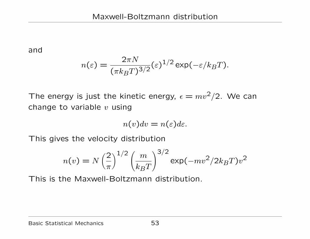
and

n(ε) =2πN

(πkBT )3/2(ε)1/2 exp(−ε/kBT ).

The energy is just the kinetic energy, ε = mv2/2. We can

change to variable v using

n(v)dv = n(ε)dε.

This gives the velocity distribution

n(v) = N

(2

π

)1/2(m

kBT

)3/2

exp(−mv2/2kBT )v2

This is the Maxwell-Boltzmann distribution.


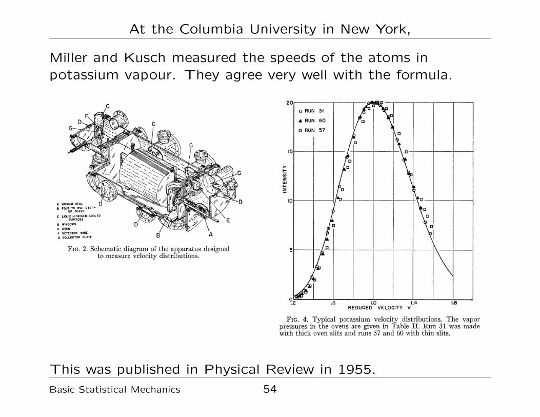
At the Columbia University in New York,

Miller and Kusch measured the speeds of the atoms inpotassium vapour. They agree very well with the formula.

This was published in Physical Review in 1955.


When would it break down?

We have assumed that: ”It is extremely unlikely that twoatoms would ever occupy the same energy state.”

Recall that we have arrived at this by looking at the number ofstates below the mean energy 3kBT/2, when T is at roomtemperature.

If T is very small, there may be far fewer states below the meanenergy. Then it would be very likely for two atoms to occupythe same state, and the Maxwell-Boltzmann distribution wouldnot be valid.

Instead, quantum statistics - such as Fermi-Dirac orBose-Einstein - have to be used. We shall learn about this.Basic Statistical Mechanics 55

Partition function.

That there is a set of formulae that we can use to find the

energy from the partition function.

The energy is given by:

U = kBT2∂ lnZN

∂T

where the many particle partition function ZN for for

indistinguishable particles is

ZN =ZNSPN !

.

(Prove it.)

Substituting this, we find

U =3NkBT

2and C =

dU

dT=

3

2NkB,

as expected from kinetic theory.


Boltzmann’s postulate

Recall that the Boltzmann distribution comes fromBoltzmann’s postulate

S = kB ln Ω.

The ability to derive the correct heat capacities forparamagnetic salts, ideal gases, and other systems are strongevidence that the postulate is correct.

Results such as the heat capacity

C =3

2NkB

can be directly measured on real gases that are nearly ideal,such as Helium.

This provides a means to obtain the Boltzmann constant,which turns out to be related to the gas constant:

kB =R

NA.


Documents

Statistical and Low Temperature Physics (PHYS393) - University of