Embed Size (px)
Citation preview

Statistical Analysis of Social Networks
1) From description to Inference: Confidence intervals for measures
2) QAP Models – (review)1) Networks as independent variables2) Networks as dependent variables
3) ERGM / Markov Chain Monte Carlo (MCMC)4) Simulations from process to network
http://www.soc.duke.edu/~jmoody77/s884/notes/stochasticNets.ppt

Statistical Analysis of Social Networks
Confidence Intervals: Bootstraps and Jackknifes(Snijders & Borgatti, 1999)
Goal: “Useful to have an indication of how precise a given description is, particularly when making comparisons between groups.”
Assumes that “a researcher is interested in some descriptive statistic … and wishes to have a standard error for this descriptive statistic without making implausibly strong assumptions about how the network came about.”
Confidence Intervals: Bootstraps and Jackknifes(Snijders & Borgatti, 1999)
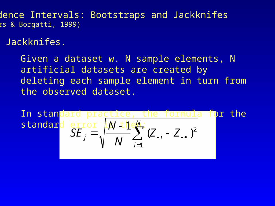
Jackknifes.
Given a dataset w. N sample elements, N artificial datasets are created by deleting each sample element in turn from the observed dataset.
In standard practice, the formula for the standard error is then:
N
iij ZZ
N
NSE
1
2)(1
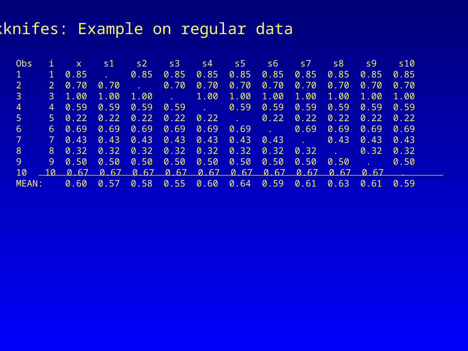
Obs i x s1 s2 s3 s4 s5 s6 s7 s8 s9 s101 1 0.85 . 0.85 0.85 0.85 0.85 0.85 0.85 0.85 0.85 0.852 2 0.70 0.70 . 0.70 0.70 0.70 0.70 0.70 0.70 0.70 0.703 3 1.00 1.00 1.00 . 1.00 1.00 1.00 1.00 1.00 1.00 1.004 4 0.59 0.59 0.59 0.59 . 0.59 0.59 0.59 0.59 0.59 0.595 5 0.22 0.22 0.22 0.22 0.22 . 0.22 0.22 0.22 0.22 0.226 6 0.69 0.69 0.69 0.69 0.69 0.69 . 0.69 0.69 0.69 0.697 7 0.43 0.43 0.43 0.43 0.43 0.43 0.43 . 0.43 0.43 0.438 8 0.32 0.32 0.32 0.32 0.32 0.32 0.32 0.32 . 0.32 0.329 9 0.50 0.50 0.50 0.50 0.50 0.50 0.50 0.50 0.50 . 0.5010 10 0.67 0.67 0.67 0.67 0.67 0.67 0.67 0.67 0.67 0.67 . MEAN: 0.60 0.57 0.58 0.55 0.60 0.64 0.59 0.61 0.63 0.61 0.59
Jackknifes: Example on regular data

Jackknifes: Example on regular data
SEj = 0.0753SE = 0.0753

Jackknifes: For networks
For networks,we need to adjust the scaling parameter:
N
iij ZZ
N
NSE
1
2)(2
2
Where Z-i is the network statistic calculated without vertex i, and Z-• is the average of Z-1 … Z-N.
This procedure will work for any network statistic Z, and UCINET will use it to test differences in network density.

Jackknifes: For networksAn example based on the Trade data. Density, Std. Errors and confidence intervals for each matrix.
DIP_DEN DIP_SEJ DIP_UB DIP_LB0.6684783 0.0636125 0.7931588 0.5437978
CRUDE_DEN CRUDE_SEJ CRUDE_UB CRUDE_LB0.5561594 0.0676669 0.6887866 0.4235323
FOOD_DEN FOOD_SEJ FOOD_UB FOOD_LB0.5561594 0.0633776 0.6803794 0.4319394
MAN_DEN MAN_SEJ MAN_UB MAN_LB0.5615942 0.0724143 0.7035263 0.4196621
MIN_DEN MIN_SEJ MIN_UB MIN_LB0.2445652 0.0530224 0.3484891 0.1406414

Bootstrap
In general, bootstrap techniques effectively treat the given sample as the population, then draw samples, with replacement, from the observed distribution.
For networks, we draw random samples of the vertices, creating a new network Y*
)()( ),()(* hikiforYY hikikh
If i(k) = i(h), then randomly fill in the dyads based from the set of all possible dyads (I.e. fill in this cell with a random draw from the population).
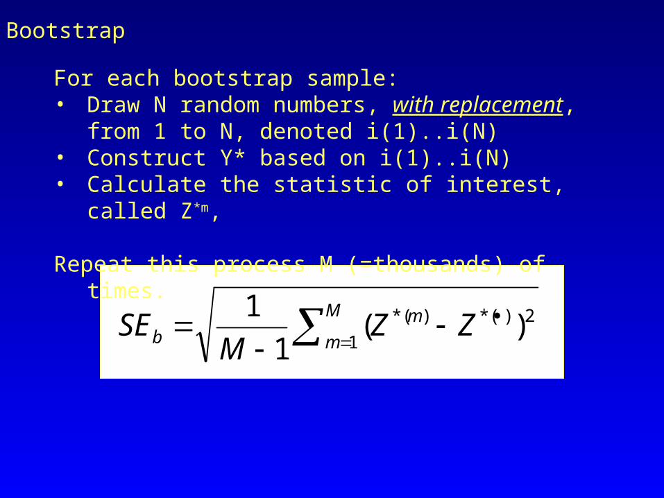
Bootstrap
For each bootstrap sample:• Draw N random numbers, with replacement, from 1 to N,
denoted i(1)..i(N)• Construct Y* based on i(1)..i(N)• Calculate the statistic of interest, called Z*m,
Repeat this process M (=thousands) of times.
M
m
mb ZZ
MSE
1
2)*()*( )(1
1
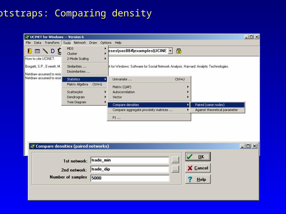
Bootstraps: Comparing density

BOOTSTRAP PAIRED SAMPLE T-TEST--------------------------------------------------------------------------------
Density of trade_min is: 0.2446Density of trade_dip is: 0.6685Difference in density is: -0.4239
Number of bootstrap samples: 5000Variance of ties for trade_min: 0.1851Variance of ties for trade_dip: 0.2220Classical standard error of difference: 0.0272Classical t-test (indep samples): -15.6096Estimated bootstrap standard error for density of trade_min: 0.0458Estimated bootstrap standard error for density of trade_dip: 0.0553Bootstrap standard error of the difference (indep samples): 0.071995% confidence interval for the difference (indep samples): [-0.5648, -0.2831]bootstrap t-statistic (indep samples): -5.8994Bootstrap SE for the difference (paired samples): 0.043095% bootstrap CI for the difference (paired samples): [-0.5082, -0.3396]t-statistic: -9.8547Average bootstrap difference: -0.3972Proportion of absolute differences as large as observed: 0.0002Proportion of differences as large as observed: 1.0000Proportion of differences as large as observed: 0.0002
Bootstraps: Comparing density

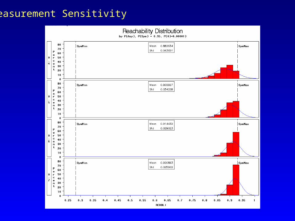
Measurement Sensitivity
A related question: How confident can you be in any measure on an observed network, given the likelihood that observed ties are, in fact, observed with error?
•Implies that some of the observed 0s are in fact 1s and some of the 1s are in fact 0s.
•Suggests that we view the network not as a binary array of 0s and 1s, but instead a set of probabilities, such that:
Pij = f(Aij)
We can then calculate the statistic of interest M times under different realizations of the network given Pij and get a distribution of the statistic of interest.

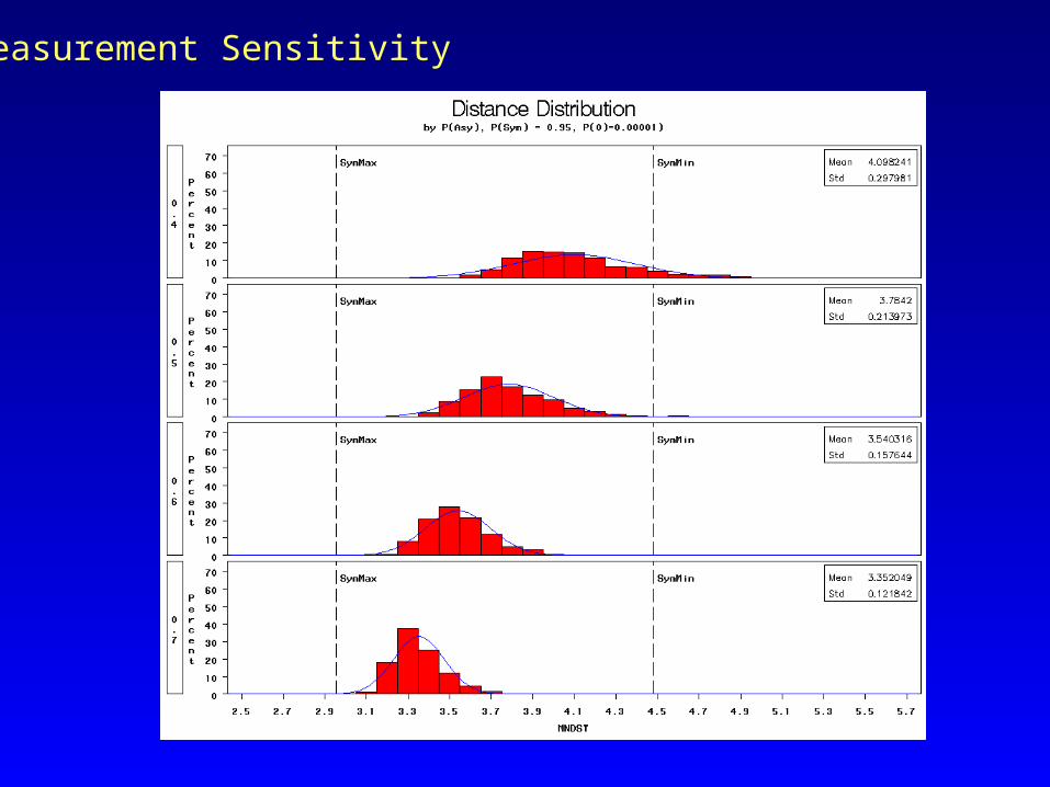
Measurement Sensitivity
It seems a reasonable approach to assessing the effect of measurement error on the ties in a network is to ask how would the network measures change if the observed ties differed from those observed. This question can be answered simply with Monte Carlo simulations on the observed network. Thus, the procedure I propose is to:
• Generate a probability matrix from the set of observed ties, • Generate many realizations of the network based on these underlying probabilities, and •Compare the distribution of generated statistics to those observed in the data.
•How do we set pij?•Range based on observed features (Sensitivity analysis)•Outcome of a model based on observed patterns (ERGM)
Measurement Sensitivity
As an example, consider the problem of defining “friendship” ties in highschools.
Should we count nominations that are not reciprocated?

Measurement Sensitivity
All ties Reciprocated
Measurement Sensitivity
Measurement Sensitivity

Measurement Sensitivity

Measurement Sensitivity

Measurement Sensitivity

Measurement Sensitivity

Statistical Analysis of Social Networks
Comparing multiple networks: QAP
The substantive question is how one set of relations (or dyadic attributes) relates to another. For example:
• Do marriage ties correlate with business ties in the Medici family network?• Are friendship relations correlated with joint membership in a club?
(review)

Assessing the correlation is straight forward, as we simply correlate each corresponding cell of the two matrices:
Marriage 1 ACCIAIUOL 0 0 0 0 0 0 0 0 1 0 0 0 0 0 0 0 2 ALBIZZI 0 0 0 0 0 1 1 0 1 0 0 0 0 0 0 0 3 BARBADORI 0 0 0 0 1 0 0 0 1 0 0 0 0 0 0 0 4 BISCHERI 0 0 0 0 0 0 1 0 0 0 1 0 0 0 1 0 5 CASTELLAN 0 0 1 0 0 0 0 0 0 0 1 0 0 0 1 0 6 GINORI 0 1 0 0 0 0 0 0 0 0 0 0 0 0 0 0 7 GUADAGNI 0 1 0 1 0 0 0 1 0 0 0 0 0 0 0 1 8 LAMBERTES 0 0 0 0 0 0 1 0 0 0 0 0 0 0 0 0 9 MEDICI 1 1 1 0 0 0 0 0 0 0 0 0 1 1 0 1 10 PAZZI 0 0 0 0 0 0 0 0 0 0 0 0 0 1 0 0 11 PERUZZI 0 0 0 1 1 0 0 0 0 0 0 0 0 0 1 0 12 PUCCI 0 0 0 0 0 0 0 0 0 0 0 0 0 0 0 0 13 RIDOLFI 0 0 0 0 0 0 0 0 1 0 0 0 0 0 1 1 14 SALVIATI 0 0 0 0 0 0 0 0 1 1 0 0 0 0 0 0 15 STROZZI 0 0 0 1 1 0 0 0 0 0 1 0 1 0 0 0 16 TORNABUON 0 0 0 0 0 0 1 0 1 0 0 0 1 0 0 0
Business 1 0 0 0 0 0 0 0 0 0 0 0 0 0 0 0 0 2 0 0 0 0 0 0 0 0 0 0 0 0 0 0 0 0 3 0 0 0 0 1 1 0 0 1 0 1 0 0 0 0 0 4 0 0 0 0 0 0 1 1 0 0 1 0 0 0 0 0 5 0 0 1 0 0 0 0 1 0 0 1 0 0 0 0 0 6 0 0 1 0 0 0 0 0 1 0 0 0 0 0 0 0 7 0 0 0 1 0 0 0 1 0 0 0 0 0 0 0 0 8 0 0 0 1 1 0 1 0 0 0 1 0 0 0 0 0 9 0 0 1 0 0 1 0 0 0 1 0 0 0 1 0 1 10 0 0 0 0 0 0 0 0 1 0 0 0 0 0 0 0 11 0 0 1 1 1 0 0 1 0 0 0 0 0 0 0 0 12 0 0 0 0 0 0 0 0 0 0 0 0 0 0 0 0 13 0 0 0 0 0 0 0 0 0 0 0 0 0 0 0 0 14 0 0 0 0 0 0 0 0 1 0 0 0 0 0 0 0 15 0 0 0 0 0 0 0 0 0 0 0 0 0 0 0 0 16 0 0 0 0 0 0 0 0 1 0 0 0 0 0 0 0
Dyads:1 2 0 01 3 0 01 4 0 01 5 0 01 6 0 01 7 0 01 8 0 01 9 1 01 10 0 01 11 0 01 12 0 01 13 0 01 14 0 01 15 0 01 16 0 02 1 0 02 3 0 02 4 0 02 5 0 02 6 1 02 7 1 02 8 0 02 9 1 02 10 0 02 11 0 02 12 0 02 13 0 02 14 0 02 15 0 02 16 0 0
Correlation:
1 0.37186790.3718679 1
(review)

Comparing multiple networks: QAP
But is the observed value statistically significant?
Can’t use standard inference, since the assumptions are violated. Instead, we use a permutation approach.
Essentially, we are asking whether the observed correlation is large (small) compared to that which we would get if the assignment of variables to nodes were random, but the interdependencies within variables were maintained.
Do this by randomly sorting the rows and columns of the matrix, then re-estimating the correlation.
(review)

Comparing multiple networks: QAP
When you permute, you have to permute both the rows and the columns simultaneously to maintain the interdependencies in the data:
ID ORIG
A 0 1 2 3 4B 0 0 1 2 3C 0 0 0 1 2D 0 0 0 0 1E 0 0 0 0 0
Sorted A 0 3 1 2 4 D 0 0 0 0 1 B 0 2 0 1 3 C 0 1 0 0 2 E 0 0 0 0 0
(review)
Comparing multiple networks: QAP
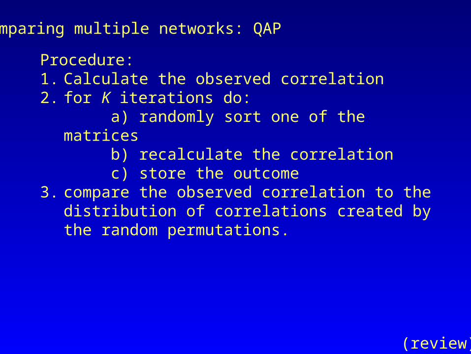
Procedure:1. Calculate the observed correlation2. for K iterations do:
a) randomly sort one of the matricesb) recalculate the correlationc) store the outcome
3. compare the observed correlation to the distribution of correlations created by the random permutations.
(review)

Comparing multiple networks: QAP
(review)

Running QAP in UCINET:
(review)
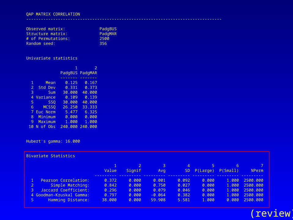
QAP MATRIX CORRELATION--------------------------------------------------------------------------------
Observed matrix: PadgBUSStructure matrix: PadgMAR# of Permutations: 2500Random seed: 356
Univariate statistics
1 2 PadgBUS PadgMAR ------- ------- 1 Mean 0.125 0.167 2 Std Dev 0.331 0.373 3 Sum 30.000 40.000 4 Variance 0.109 0.139 5 SSQ 30.000 40.000 6 MCSSQ 26.250 33.333 7 Euc Norm 5.477 6.325 8 Minimum 0.000 0.000 9 Maximum 1.000 1.000 10 N of Obs 240.000 240.000
Hubert's gamma: 16.000
Bivariate Statistics
1 2 3 4 5 6 7 Value Signif Avg SD P(Large) P(Small) NPerm --------- --------- --------- --------- --------- --------- --------- 1 Pearson Correlation: 0.372 0.000 0.001 0.092 0.000 1.000 2500.000 2 Simple Matching: 0.842 0.000 0.750 0.027 0.000 1.000 2500.000 3 Jaccard Coefficient: 0.296 0.000 0.079 0.046 0.000 1.000 2500.000 4 Goodman-Kruskal Gamma: 0.797 0.000 -0.064 0.382 0.000 1.000 2500.000 5 Hamming Distance: 38.000 0.000 59.908 5.581 1.000 0.000 2500.000
(review)

Running QAP in UCINET: RegressionUsing the same logic,we can estimate alternative models, such as regression. Only complication is that you need to permute all of the independent matrices in the same way each iteration.
(review)
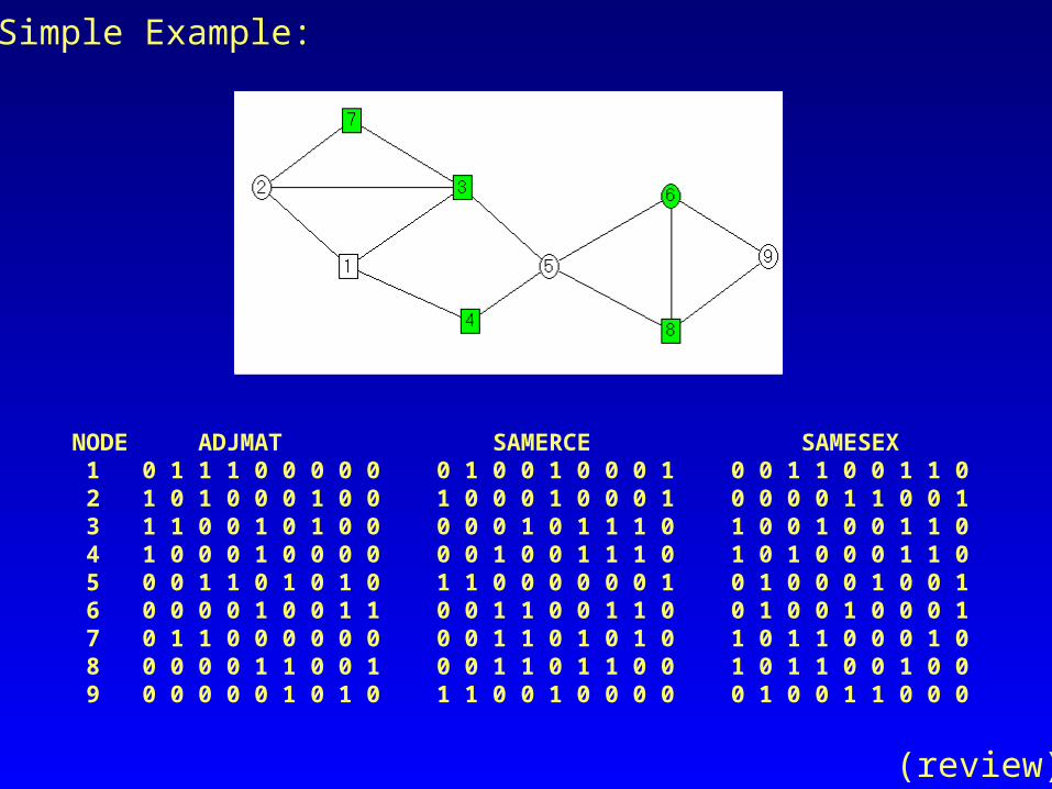
NODE ADJMAT SAMERCE SAMESEX 1 0 1 1 1 0 0 0 0 0 0 1 0 0 1 0 0 0 1 0 0 1 1 0 0 1 1 0 2 1 0 1 0 0 0 1 0 0 1 0 0 0 1 0 0 0 1 0 0 0 0 1 1 0 0 1 3 1 1 0 0 1 0 1 0 0 0 0 0 1 0 1 1 1 0 1 0 0 1 0 0 1 1 0 4 1 0 0 0 1 0 0 0 0 0 0 1 0 0 1 1 1 0 1 0 1 0 0 0 1 1 0 5 0 0 1 1 0 1 0 1 0 1 1 0 0 0 0 0 0 1 0 1 0 0 0 1 0 0 1 6 0 0 0 0 1 0 0 1 1 0 0 1 1 0 0 1 1 0 0 1 0 0 1 0 0 0 1 7 0 1 1 0 0 0 0 0 0 0 0 1 1 0 1 0 1 0 1 0 1 1 0 0 0 1 0 8 0 0 0 0 1 1 0 0 1 0 0 1 1 0 1 1 0 0 1 0 1 1 0 0 1 0 0 9 0 0 0 0 0 1 0 1 0 1 1 0 0 1 0 0 0 0 0 1 0 0 1 1 0 0 0
Simple Example:
(review)

Distance (Dij=abs(Yi-Yj).000 .277 .228 .181 .278 .298 .095 .307 .481.277 .000 .049 .096 .555 .575 .182 .584 .758.228 .049 .000 .047 .506 .526 .134 .535 .710.181 .096 .047 .000 .459 .479 .087 .488 .663.278 .555 .506 .459 .000 .020 .372 .029 .204.298 .575 .526 .479 .020 .000 .392 .009 .184.095 .182 .134 .087 .372 .392 .000 .401 .576.307 .584 .535 .488 .029 .009 .401 .000 .175.481 .758 .710 .663 .204 .184 .576 .175 .000
Y 0.32 0.59 0.54 0.50 0.04 0.02 0.41 0.01-0.17
Simple Example:
(review)

Simple Example:
(review)

Simple Example, continuous dep. variable:# of permutations: 2000Diagonal valid? NORandom seed: 995Dependent variable: EX_SIMExpected values: C:\moody\Classes\soc884\examples\UCINET\mrqap-predictedIndependent variables: EX_SSEX EX_SRCE EX_ADJ
Number of valid observations among the X variables = 72N = 72
Number of permutations performed: 1999
MODEL FITR-square Adj R-Sqr Probability # of Obs-------- --------- ----------- ----------- 0.289 0.269 0.059 72
REGRESSION COEFFICIENTS
Un-stdized Stdized Proportion Proportion Independent Coefficient Coefficient Significance As Large As Small ----------- ----------- ----------- ------------ ----------- ----------- Intercept 0.460139 0.000000 0.034 0.034 0.966 EX_SSEX -0.073787 -0.170620 0.140 0.860 0.140 EX_SRCE -0.020472 -0.047338 0.272 0.728 0.272 EX_ADJ -0.239896 -0.536211 0.012 0.988 0.012
(review)

We can also model the network as a dependent variable. In the next example, I model diplomacy as a function of trade, using the country data.
Note that using UCINET, this gives a linear probability model, OLS on a 0-1 dependent variable. This is often not optimal…
(review)

MULTIPLE REGRESSION QAP TRADE DIPLOMACY--------------------------------------------------------------------------------# of permutations: 2000Diagonal valid? NORandom seed: 1000Dependent variable: trade_dipExpected values: C:\moody\Classes\soc884\examples\UCINET\mrqap-predictedIndependent variables: TRADE_FOOD TRADE_CRUDE TRADE_MAN TRADE_MIN
Number of valid observations among the X variables = 552N = 552Number of permutations performed: 1999
MODEL FITR-square Adj R-Sqr Probability # of Obs-------- --------- ----------- ----------- 0.317 0.314 0.000 552
REGRESSION COEFFICIENTS Un-stdized Stdized Proportion Proportion Independent Coefficient Coefficient Significance As Large As Small -------------- ----------- ----------- ------------ ----------- ----------- Intercept 0.339308 0.000000 1.000 1.000 0.000 TRADE_FOOD 0.049975 0.052744 0.200 0.200 0.800 TRADE_CRUDE 0.109233 0.115284 0.033 0.033 0.967 TRADE_MAN 0.367435 0.387285 0.000 0.000 1.000 TRADE_MIN 0.140151 0.127965 0.058 0.058 0.942
Expected values saved as dataset mrqap-predictedValid observations saved as dataset mrqap-valid
(review)

One solution is to use a QAP Logit model. Note (yet) implemented in UCINET, but you can use DAMN or SAS. Let’s look at the country trade data again, using a logit model.
DAMN *** REGRESSION PARAMETERS *** man coefficient= 1.80356 p-value=0.00000 food coefficient= 0.30928 p-value=0.14867 crude coefficient= 0.59624 p-value=0.00867 min coefficient= 1.61641 p-value=0.00000 constant coefficient= -0.78063 p-value=0.00000 Final Likelihood: -252.366402
QAP Results: Logit model coefficientsSignificance results are equal to the proportion of QAP parameters
that are as *small* as the observed parameters.
PARAMETERS COEF SIGINTERCEPT -.949 .0010TMAN 1.863 .9980TFOOD .3914 .8420TCRUDE .6667 .9800TMIN 1.658 .9980
(review)
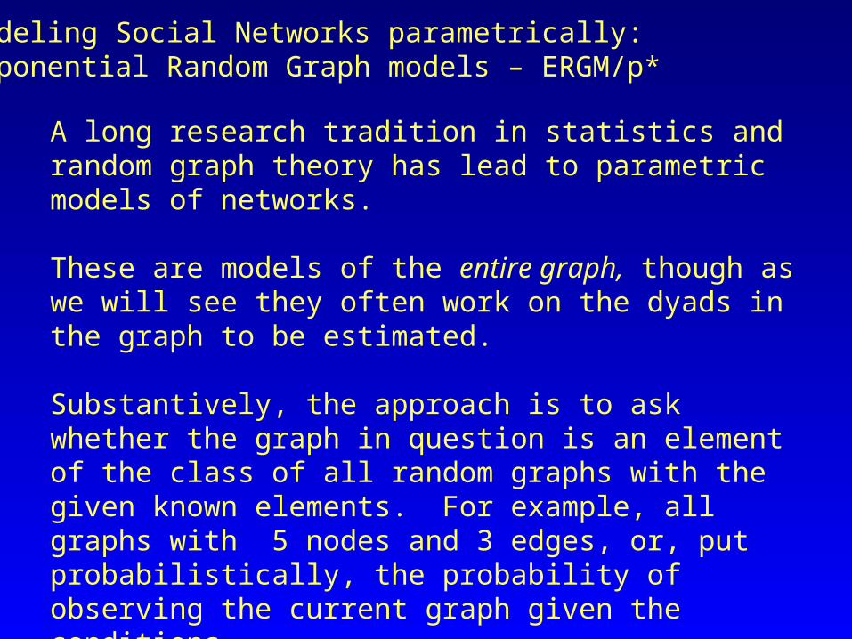
Modeling Social Networks parametrically:Exponential Random Graph models – ERGM/p*
A long research tradition in statistics and random graph theory has lead to parametric models of networks.
These are models of the entire graph, though as we will see they often work on the dyads in the graph to be estimated.
Substantively, the approach is to ask whether the graph in question is an element of the class of all random graphs with the given known elements. For example, all graphs with 5 nodes and 3 edges, or, put probabilistically, the probability of observing the current graph given the conditions.

Random Graphs and Conditional Expectations
The basis for the statistical modeling of graphs rests on random graph theory.
Simply put, Random graph theory asks what properties do we expect when ties (Xij) form at random.
The simplest random graph is the Bernoulli random graph, where Xij is a constant and independent: says simply that each edge in the graph has an independent probability of being 1/0.
Typically this is an uninteresting distribution of graphs, and we want to know what the graph looks like conditional on other features of the graph.

Random Graphs and Conditional Expectations
A Bernoulli graph is only conditional on the expected number of edges. So effectively we ask “What is the probability of observing the graph we have, given the set of all possible graphs with the same number of edges.”
We might, instead, want to condition on the degree distribution (sent or received) or all graphs with a particular dyad distribution (same number of Mutual, Asymmetric and Null dyads).
Closed form solutions for some graph statistics (like the triad census) are known for out-degree, in-degree and MAN (but not all 3 simultaneously).

Random Graphs and Conditional Expectations
PAJEK gives you the unconditional expected values:
------------------------------------------------------------------------------Triadic Census 2. i:\people\jwm\s884\homework\prison.net (67)------------------------------------------------------------------------------ Working...---------------------------------------------------------------------------- Type Number of triads (ni) Expected (ei) (ni-ei)/ei---------------------------------------------------------------------------- 1 - 003 39221 37227.47 0.05 2 - 012 5860 9587.83 -0.39 3 - 102 2336 205.78 10.35 4 - 021D 61 205.78 -0.70 5 - 021U 80 205.78 -0.61 6 - 021C 103 411.55 -0.75 7 - 111D 105 17.67 4.94 8 - 111U 69 17.67 2.91 9 - 030T 13 17.67 -0.26 10 - 030C 1 5.89 -0.83 11 - 201 12 0.38 30.65 12 - 120D 15 0.38 38.56 13 - 120U 7 0.38 17.46 14 - 120C 5 0.76 5.59 15 - 210 12 0.03 367.67 16 - 300 5 0.00 21471.04 ---------------------------------------------------------------------------- Chi-Square: 137414.3919*** 6 cells (37.50%) have expected frequencies less than 5. The minimum expected cell frequency is 0.00.

Random Graphs and Conditional Expectations
SPAN gives you the (X|MAN) distributions:
Triad Census T TPCNT PU EVT VARTU STDDIF
003 39221 0.8187 0.8194 39251 427.69 -1.472012 5860 0.1223 0.1213 5810.8 1053.5 1.5156102 2336 0.0488 0.0476 2278.7 321.01 3.1954021D 61 0.0013 0.0015 70.949 67.37 -1.212021U 80 0.0017 0.0015 70.949 67.37 1.1027021C 103 0.0022 0.003 141.9 127.58 -3.444111D 105 0.0022 0.0023 112.39 103.57 -0.727111U 69 0.0014 0.0023 112.39 103.57 -4.264030T 13 0.0003 0.0001 3.4292 3.3956 5.1939030C 1 209E-7 239E-7 1.1431 1.1393 -0.134201 12 0.0003 0.0009 42.974 38.123 -5.017120D 15 0.0003 286E-7 1.3717 1.368 11.652120U 7 0.0001 286E-7 1.3717 1.368 4.8122120C 5 0.0001 573E-7 2.7433 2.7285 1.3662210 12 0.0003 442E-7 2.1186 2.1023 6.8151300 5 0.0001 549E-8 0.2631 0.2621 9.2522

Modeling Social Networks parametrically:ERGM approaches
The earliest approaches are based on simple random graph theory, but there’s been a flurry of activity in the last 10 years or so.
Key historical references:- Holland and Leinhardt (1981) JASA- Frank and Strauss (1986) JASA- Wasserman and Faust (1994) – Chap 15 & 16-Wasserman and Pattison (1996)
Best current update: http://www.jstatsoft.org/v24

Modeling Social Networks parametrically:ERGM approaches
The “p1” model of Holland and Leinhardt is the classic foundation – the basic idea is that you can generate a statistical model of the network by predicting the counts of types of ties (asym, null, sym). They formulate a log-linear model for these counts; but the model is equivalent to a logit model on the dyads:
)(1Xlogit ij jiji X
Note the subscripts! This implies a distinct parameter for every node i and j in the model, plus one for reciprocity.

Modeling Social Networks parametrically:ERGM approaches
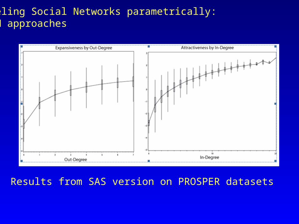
Modeling Social Networks parametrically:ERGM approaches
Results from SAS version on PROSPER datasets

Modeling Social Networks parametrically:ERGM approaches
Once you know the basic model format, you can imagine other specifications:
(orig) chars) (node )(1Xlogit
y)reciprocit ial(different )(1Xlogit
(orig) )(1Xlogit
ij
ij
ij
jiji
jigji
jiji
X
X
X
Key is to ensure that the specification doesn’t imply a linear dependency of terms.
Model fit is hard to judge – newer work shows that the se’s are “approximate” ;-)

)(
)}(exp{)(
xz
xXp
Where: is a vector of parameters (like regression coefficients)z is a vector of network statistics, conditioning the graph is a normalizing constant, to ensure the probabilities sum to 1.
Modeling Social Networks parametrically:ERGM approaches

)(
}exp{
)( ,
ji
ijij x
xXp
The simplest graph is a Bernoulli random graph,where each Xij is independent:
Where:
ij = logit[P(Xij = 1)]
() =[1 + exp(ij )]
Note this is one of the few cases where () can be written.
Modeling Social Networks parametrically:ERGM approaches
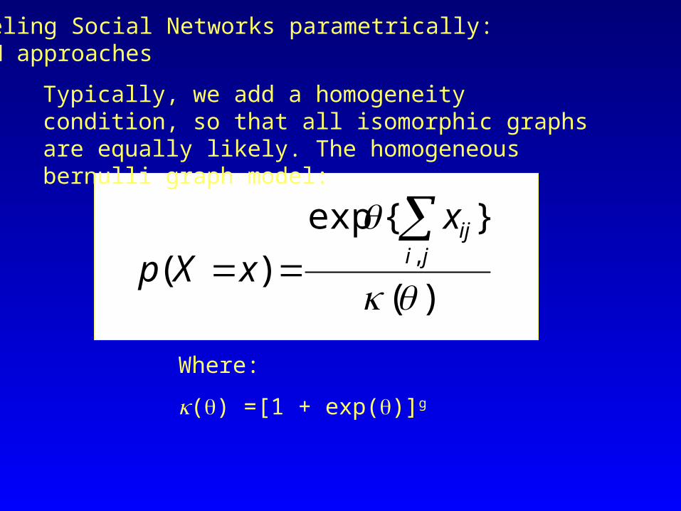
Typically, we add a homogeneity condition, so that all isomorphic graphs are equally likely. The homogeneous bernulli graph model:
)(
}{exp
)( ,
ji
ijx
xXp
Where:
() =[1 + exp()]g
Modeling Social Networks parametrically:ERGM approaches

If we want to condition on anything much more complicated than density, the normalizing constant ends up being a problem. We need a way to express the probability of the graph that doesn’t depend on that constant. First some terms:
j and ibetween tienox with Sociomatri
0 toforcedelement ijx with Sociomatri
1 toforcedelement ijx with Sociomatri
,
,
,
cji
ji
ji
X
X
X
Modeling Social Networks parametrically:ERGM approaches

)|0(
)|1()exp(
cijij
cijij
ij XXp
XXpw
)]()([exp{
)}(exp{
)}(exp{
)|0(
)|1(
ijij
ij
ij
cijij
cijij
xzxz
xz
xz
XXp
XXp
)]()([)|0(
)|1(log
ijijcijij
cijij
ij xzxzXXp
XXp
Modeling Social Networks parametrically:ERGM approaches
)]()([)|0(
)|1(log
ijijcijij
cijij
ij xzxzXXp
XXp
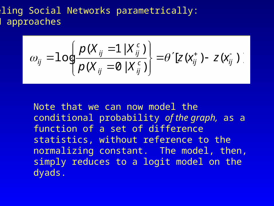
Note that we can now model the conditional probability of the graph, as a function of a set of difference statistics, without reference to the normalizing constant. The model, then, simply reduces to a logit model on the dyads.
Modeling Social Networks parametrically:ERGM approaches

Modeling Social Networks parametrically:ERGM approaches
)]()([)|0(
)|1(log
ijijcijij
cijij
ij xzxzXXp
XXp
Consider the simplest possible model: the Bernoulli random graph model, which says the only feature of interest is the number of edges in the graph. What is the change statistic for that feature?
dyads) allfor 1 is e(differenc 1][
zero) is vakyeso absent, is edge (assume )0(
one) is valueso present, is edge (assume )1(
ijij
ij
ij
xxz
xz
xz

Modeling Social Networks parametrically:ERGM approaches
Consider the simplest possible model: the Bernoulli random graph model, which says the only feature of interest is the number of edges in the graph. What is the change statistic for that feature?
The “Edges” parameter is simply an intercept-only model.
NODE ADJMAT
1 0 1 1 1 0 0 0 0 0
2 1 0 1 0 0 0 1 0 0
3 1 1 0 0 1 0 1 0 0
4 1 0 0 0 1 0 0 0 0
5 0 0 1 1 0 1 0 1 0
6 0 0 0 0 1 0 0 1 1
7 0 1 1 0 0 0 0 0 0
8 0 0 0 0 1 1 0 0 1
9 0 0 0 0 0 1 0 1 0
Density: 0.311

Modeling Social Networks parametrically:ERGM approaches
Consider the simplest possible model: the Bernoulli random graph model, which says the only feature of interest is the number of edges in the graph. What is the change statistic for that feature?
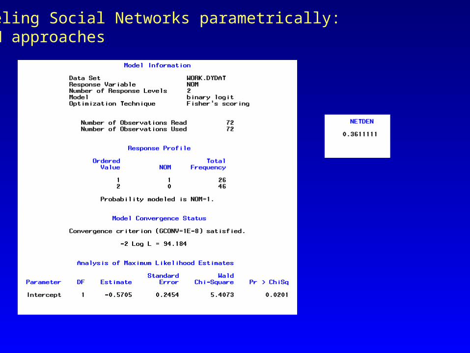
The “Edges” parameter is simply an intercept-only model.
proc logistic descending data=dydat;
model nom =;
run; quit;
---see results copy coef ---
data chk;
x=exp(-0.5705)/(1+exp(-0.5705));
run;
proc print data=chk;
run;
Modeling Social Networks parametrically:ERGM approaches

Including: A Practical Guide To Fitting p* Social Network
ModelsVia Logistic Regression
The site includes the PREPSTAR program for creating the variables of interest. The following example draws from this work. – this bit nicely walks you through the logic of constructing change variables, model fit and so forth.
But the estimates are not very good for any parameters other than “dyad independent” parameters!
Modeling Social Networks parametrically:ERGM approaches
The logit model estimation procedure was popularized by Wasserman & colleagues, and a good guide to this approach is:

Modeling Social Networks parametrically:ERGM approaches
Parameters that are often fit include:1) Expansiveness and attractiveness parameters. = dummies for
each sender/receiver in the network2) Degree distribution 3) Mutuality 4) Group membership (and all other parameters by group)5) Transitivity / Intransitivity6) K-in-stars, k-out-stars7) Cyclicity8) Node-level covariates (Matching, difference)9) Edge-level covariates (dyad-level features such as exposure)10) Temporal data – such as relations in prior waves.

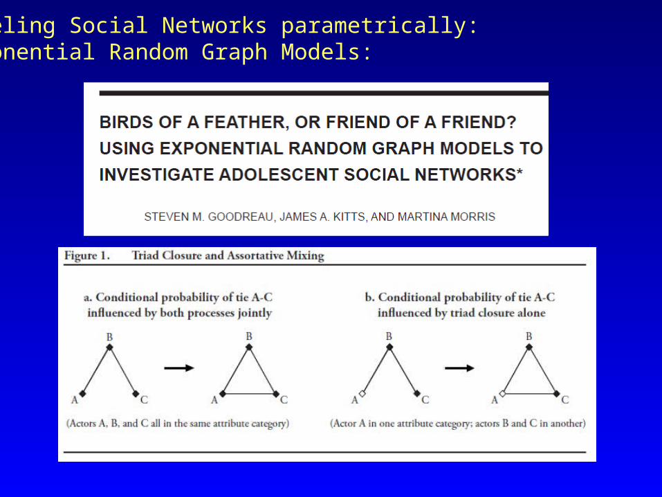
Modeling Social Networks parametrically:Exponential Random Graph Models

Modeling Social Networks parametrically:Exponential Random Graph Models
…and there are LOTS of terms…

-0.6
-0.4
-0.2
0
0.2
0.4
0.6
0.8
Same Race
SES
GPA
Both Smoke
College
Drinking
FightReciprocity
Same Sex
Same Clubs
Transitivity
Intransitivity
Same Grade
Network Model Coefficients, In school Networks
Complete Network AnalysisStochastic Network Analysis An example:

Modeling Social Networks parametrically:Exponential Random Graph Models
In practice, logit estimated models are difficult to estimate, and we have no good sense of how approximate the PMLE is.
The STATNET generalization is to use MCMC methods to better estimate the parameters. This is essentially a simulation procedure working “under the hood” to explore the space of graphs described by the model parameters; searching for the best fit to the observed data.

Modeling Social Networks parametrically:Exponential Random Graph Models
You can specify a model as a simple statement on terms:

Modeling Social Networks parametrically:Exponential Random Graph Models
Modeling Social Networks parametrically:Exponential Random Graph Models:

Modeling Social Networks parametrically:Exponential Random Graph Models:

Modeling Social Networks parametrically:Exponential Random Graph Models:
Example 2: Hierarchy & Context in AH
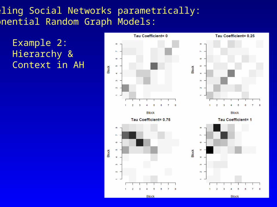
Modeling Social Networks parametrically:Exponential Random Graph Models:
Example 2: Hierarchy & Context in AH
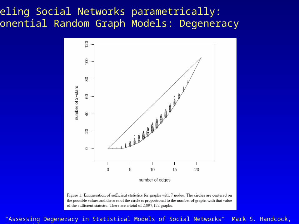
Modeling Social Networks parametrically:Exponential Random Graph Models: Degeneracy
"Assessing Degeneracy in Statistical Models of Social Networks" Mark S. Handcock, CSSS Working Paper #39

Modeling Social Networks parametrically:Exponential Random Graph Models: Degeneracy
"Assessing Degeneracy in Statistical Models of Social Networks" Mark S. Handcock, CSSS Working Paper #39

Modeling Social Networks parametrically:Exponential Random Graph Models: Degeneracy
"Assessing Degeneracy in Statistical Models of Social Networks" Mark S. Handcock, CSSS Working Paper #39

Generating Random Graph Samples
A conceptual merge between exponential random graph models and QAP/sensitivity models is to attempt to identify a sample of graphs from the universe you are trying to model.
)(
)}(exp{)(
xz
xXp
That is, generate X empirically, then compare z(x) to see how likely a measure on x would be given X. The difficulty, however, is generating X.

Generating Random Graph Samples
The first option would be to generate all isomorphic graphs within a given constraint.
This is possible for small graphs, but the number gets large fast. For a network with 3 nodes, there are 16 possible directed graphs. For a network with 4 nodes, there are 218, for 5 nodes 9608, for 6 nodes1,540,944, and so on…
So, the best approach is to sample from the universe, but, of course, if you had the universe you wouldn’t need to sample from it. How do you sample from a population you haven’t observed?
(a) use a construction algorithm that generates a random graph with known constraints (b) use a ERGM model like above.

Generating Random Graph Samples
Tom Snijders has a program called ZO (Zero-One) for doing this.
http://stat.gamma.rug.nl/snijders/
The program only works well for smallish networks (less than ~100)

Generating Random Networks with Structural Constraints.
General strategy: Assign arcs at random within the cells of an adjacency matrix until the desired graph is achieved.
Process.1) Define the pool of open arcs. Any cells of the g by g matrix which are structurally zero are not allowed.
5
3
4
5
1
3
0
2
6
7
5 3 4 51 3 0 267
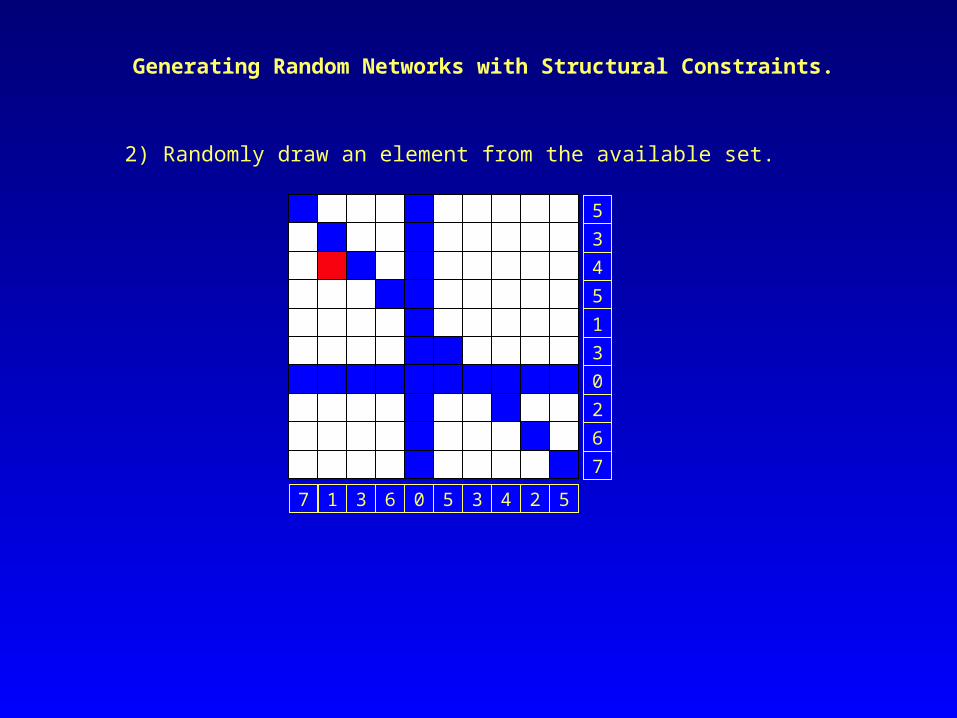
Generating Random Networks with Structural Constraints.
2) Randomly draw an element from the available set.
5
3
4
5
1
3
0
2
6
7
5 3 4 51 3 0 267

Generating Random Networks with Structural Constraints.
5
3
4
5
1
3
0
2
6
7
5 3 4 51 3 0 267
3) Check to see if selected cell meets the structural condition.
4) If a condition is met,then remove any implicated cells from the pool.
5
3
4
5
1
3
0
2
6
7
5 3 4 51 3 0 267

5) Check for Identification: Does the last arc imply the set of arcs for another?
5
3
4
5
1
3
0
2
6
7
5 3 4 51 3 0 267
Generating Random Networks with Structural Constraints.
In this example, there are only 7 available spots left in the last row, equal to the number needed to fill that row condition.

Generating Random Networks with Structural Constraints.
Process: 1) Identify the pool of open cells. 2) Randomly draw an arc from this pool. 3) Check the structural conditions against this arc. 4) If structural conditions are met, then remove implied cells from
the pool. 5) Check for identification of other arcs.
Types of constraints:• Structural Patterns, such as the in and out degree,
prohibition against cycles, etc. • Category Mixing Constraints. Nodes in category i restricted to nodes from category j.• Event Counts. Number of mutual arcs, number of ties between group i and j, etc.

Social Relations at “Holy Trinity” School.
7th Grade
8th Grade
9th Grade
10th Grade
11th Grade
12th Grade
g = 74l = 466 = .086M=108Transitivity: .357Mean Degree: 6.3
0
50
100
150
200
250
Num
ber
of N
etw
ork
s
5 10 15 20 25 30 35 40
Number of Mutual Dyads
Z.O.
RANFIX
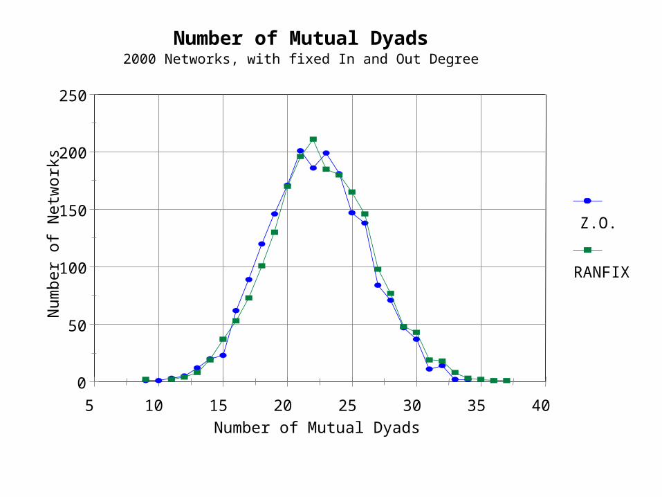
Number of Mutual Dyads2000 Networks, with fixed In and Out Degree

Distribution of Selected Triad TypesSimulations compared to Observed
0
50
100
150
200
250
300
350 C
ou
nt
300210120C120U120D201030T
Z.O.
RANFIX
Observed.
2000 random networks, with fixed in and out degree.

Romantic Networks

Romantic Networks