Statistical Analysis of Musical Instruments

Namunu Chinthaka Maddage1, Changsheng Xu1, Chin-Hui LEE2, Mohan Kankanhalli2

and Qi Tian1

1 Lab for Information Technology, 21 Heng Mui Keng Terrace Singapore 119613

maddage, xucs, tian@lit.a-star.edu.sg 2 Dept of Computer Science, National University of Singapore

Singapore 117543 chl, mohan@comp.nus.edu.sg

Abstract. One important field in the research of computer music concerns the modeling of sounds. In order to design digital models mirroring as closely as possible a real sound and permitting in addition transformation by altering the synthesis parameters. We look for a signal model based on additive synthesis, whose parameters are estimated by the analysis of real sound. In this paper we present model-based analysis of musical notes generated by electric guitar. Both time domain and frequency domain feature analysis has been performed to find out the parameter selections for the musical signal analysis. Finally, non-parametric classification technique i.e. Nearest Neighbor Rule has been utilized to classify musical notes with this best set of parameters of the musical features.

1. Introduction

Music content analysis in general has many practical applications, including structured coding, database retrieval systems, automatic musical signal annotation, and as a musicians’ tools. A subtask of this, automatic musical instruments identification is of significant importance in solving these problems and is likely to provide useful information also in the sound source identification applications, such as speaker recognition. However musical signal analysis has not been able to attain as much commercial interests as for instance, speaker and speech recognition.

First attempts in musical instrument recognition operated with a very limited number of instruments. De Poli and Prandoni used mel-frequency cepstum coefficients calculated from isolated tones as inputs to a Kohonen self-organizing map, in order to construct timber spaces [1]. Kaminsky and Materka used features derived from an rms-energy envelope and used neural network or a k-nearest neighbor rule classifier to classify guitar, piano, marimba and accordion tones over a one octave band [2].

The recent works have already shown a considerable level of performance, but have still been able to cope with only a limited amount of test data. In [3], Martin reported a

system that operated on single isolated tones played over full pitch ranges of 15 orchestral instruments and uses a hierarchical classification framework. Brown [4] and Martin [5] have managed to build classifiers that are able to operate on test data that include samples played by several different instruments of a particular instrument class, and recorded in environments, which are noisy and reverberant. However, recent systems are characterized either with a limited context or with a rather unsatisfactory performance.

Since 8-prominent musical notes in an octave generate the musical score, in this paper we experiment to find out the best selection of both musical features and their dynamic parameters, which could be the foundation for further research work on music signals. We utilized both time domain and frequency domain features to characterize the different properties of middle scale musical notes generated by an electric guitar (low noise & high amplification string type instrument)

2. Musical Scales

A musical scale is a logarithmic organization of pitch based on the octave, which is the perceived distance between two pitches when one is twice the frequency of other. For example, middle C (C4) has frequency 261.6 Hz; the octave above (C5) is 523.2 Hz and above that is soprano high C (C6) at 1046.4 Hz. The octave below middle C (C3) is 130.8 Hz, and below that, at 65.4 Hz is C2.

Although the octave seems to be a perceptual unit in humans [6], pitch organization within the octave takes different forms across cultures. In western music, the primary organization since the time of Bach has been the equal-tempered scale, which divides the octave into twelve equally spaced semitones. The octave interval corresponds to a frequency doubling and semitones are equally spaced in a multiplicative sense, so ascending one semitone multiplies the frequency by the twelfth root of 2, or approximately 1.059. The smallest pitch difference between two consecutive tones that can be perceived by humans is about 3 Hz.

3. Feature Extraction and Experimental Setup

Figure 1 Block diagram of feature extraction

Zero Crossing Spectral Power

Musical notes Digital Filter bank LPC Co -efficient

MFCC

Feature selection is important for music content analysis. Selected features should reflect the significant characteristics of different kinds of musical signals. We have selected some of the features (Figure 1) to find out how good are they, for musical signal processing.

3.1. Musical Notes

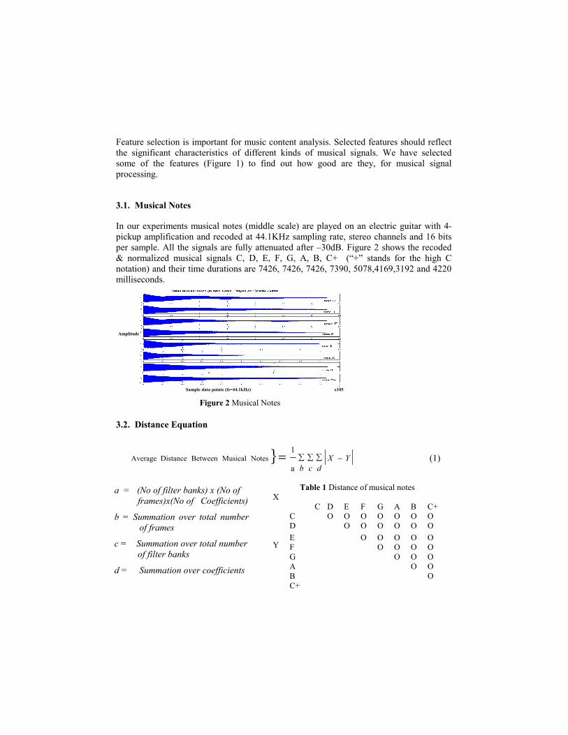
In our experiments musical notes (middle scale) are played on an electric guitar with 4-pickup amplification and recoded at 44.1KHz sampling rate, stereo channels and 16 bits per sample. All the signals are fully attenuated after –30dB. Figure 2 shows the recoded & normalized musical signals C, D, E, F, G, A, B, C+ (“+” stands for the high C notation) and their time durations are 7426, 7426, 7426, 7390, 5078,4169,3192 and 4220 milliseconds.

3.2. Distance Equation

∑ ∑ ∑ −=b c d

YXa

1Notes MusicalBetween Distance Average

(1)

Sample data points (fs=44.1kHz) x105

Figure 2 Musical Notes

Amplitude

a = (No of filter banks) x (No of frames)x(No of Coefficients)

b = Summation over total number of frames

c = Summation over total number of filter banks

d = Summation over coefficients

Table 1 Distance of musical notesX

C D E F G A B C+ C O O O O O O O D O O O O O O E O O O O O F O O O O G O O O A O O B O

Y

C+

Equation (1) calculates the average distance between musical notes sequence given above in the Table 1. X & Y are the feature vectors of musical notes and we calculate the distances between musical notes (C-D, C-E, C-F…B-C+). When average distances related to either diff-filter banks or diff-order of features are higher, then musical notes are comparatively far from each other in that filter or feature order. (i.e. Identical Musical Note Features).

3.3. Digital Filter Bank

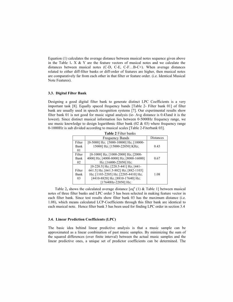
Designing a good digital filter bank to generate distinct LPC Coefficients is a very important task [8]. Equally spaced frequency bands [Table 2- Filter bank 01] of filter bank are usually used in speech recognition systems [7]. Our experimental results show filter bank 01 is not good for music signal analysis (ie- Avg distance is 0.43and it is the lowest). Since distinct musical information lies between 0-5000Hz frequency range, we use music knowledge to design logarithmic filter bank (02 & 03) where frequency range 0-1000Hz is sub divided according to musical scales [Table 2-Fiterbank 03].

Table 2, shows the calculated average distance [eqn (1) & Table 1] between musical notes of three filter banks and LPC order 5 has been selected in making feature vector in each filter bank. Since test results show filter bank 03 has the maximum distance (i.e. 1.08), which means calculated LCP-Coefficients through this filter bank are identical to each musical note. Hence filter bank 3 has been used for finding LPC order in section 3.4

3.4. Linear Prediction Coefficients (LPC)

The basic idea behind linear predictive analysis is that a music sample can be approximated as a linear combination of past music samples. By minimizing the sum of the squared differences (over finite interval) between the actual music samples and the linear predictive ones, a unique set of predictor coefficients can be determined. The

Table 2 Filter banks Frequency Bands Distances

Filter Bank

01

[0-5000] Hz; [5000-10000] Hz; [10000-15000] Hz; [15000-22050] KHz;

0.43

Filter Bank

02

[0-1000] Hz; [1000-2000] Hz; [2000-4000] Hz; [4000-8000] Hz; [8000-16000]

Hz; [16000-22050] Hz;

0.67

Filter Bank

03

[0-220.5] Hz; [220.5-441] Hz; [441-661.5] Hz; [661.5-882] Hz; [882-1103] Hz; [1103-2205] Hz; [2205-4410] Hz;

[4410-8820] Hz; [8810-17640] Hz; [17640Hz-22050] Hz;

1.08

importance of linear prediction lies in the accuracy with which the basic model applies to musical signals [10-11]. Selecting the order of LPC coefficients such that set of the values are as identical as possible to each musical note, is tough challenge, when the signal is complex. Unlike musical signals, in speech recognition, the order (6-10) is enough to distinguish the speech signals.

In Figure 3, we have plotted our experiment results of the average distance [eqn (1) & Table 1] vary with the order of LPC. Order 12 is the best set found where the average distance (i.e-1.87) is higher than other LPC orders.

Figure 4 shows how coefficient 01 of LPC order 12 of digital filter 1,2,3 & 8 of filter bank 03 varies with 20ms time frames. Mean values of all musical notes in coefficient 01 of filter 01 are above 1.00 and the variances in note C+ and B are much higher than the other notes. Note C & E are having lowest variance and both mean and variance are nearly same in each other. So distinguishing note C and E using coefficient 01 of filter 01 is difficult. Mean values of Coefficient 01 of filters 2, 3 & 8, of all musical notes are around 1.1~2.05 and variances are around 0.07~0.36. Since the variation of these coefficients identical to each musical note, they are more significant in distinguishing musical notes

3.5. Mel-frequency Cepstrum Coefficients (MFCC)

The Mel-frequency Cepstrum has proven to be highly effective in automatic speech recognition and in modeling the subjective pitch and frequency content of audio signals[11]. The mel-cepstral features can be illustrated by the Mel-Frequency Cepstral Coefficients (MFCCs), which are computed from the FFT power coefficients. The power coefficients are filtered by a triangular band pass filter bank. The filter bank consists of K=19 triangular filters. They have a constant mel-frequency interval, and covers the frequency range of 0Hz – 20050Hz. Our test results show that order 9, which gives the maximum avg-distance [eqn (1) & Table 1] (0.1378) over the order range (2 to25), is the best order for the frequency domain analysis.

Figure 4 LPC coefficients vs. time frames

Figure 3 LPC order vs. distances of musical notes

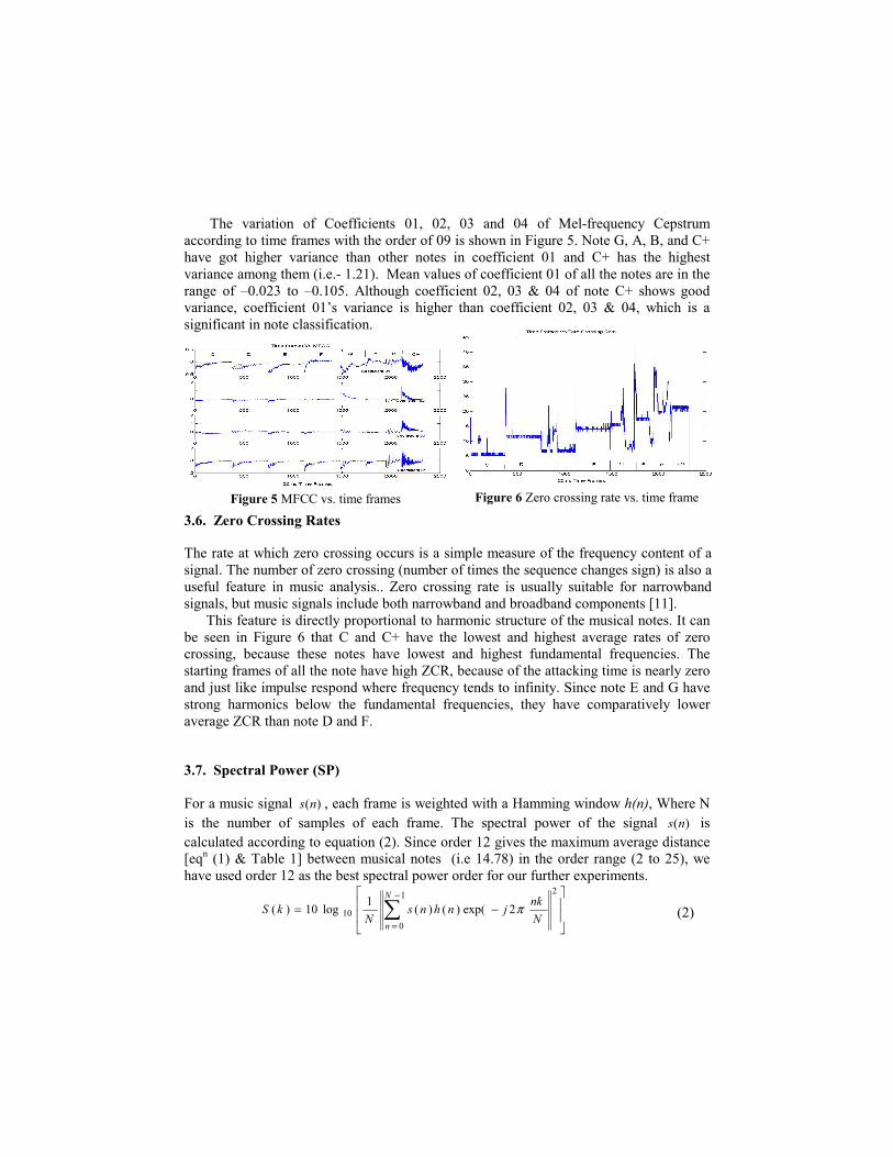
The variation of Coefficients 01, 02, 03 and 04 of Mel-frequency Cepstrum according to time frames with the order of 09 is shown in Figure 5. Note G, A, B, and C+ have got higher variance than other notes in coefficient 01 and C+ has the highest variance among them (i.e.- 1.21). Mean values of coefficient 01 of all the notes are in the range of –0.023 to –0.105. Although coefficient 02, 03 & 04 of note C+ shows good variance, coefficient 01’s variance is higher than coefficient 02, 03 & 04, which is a significant in note classification.

3.6. Zero Crossing Rates

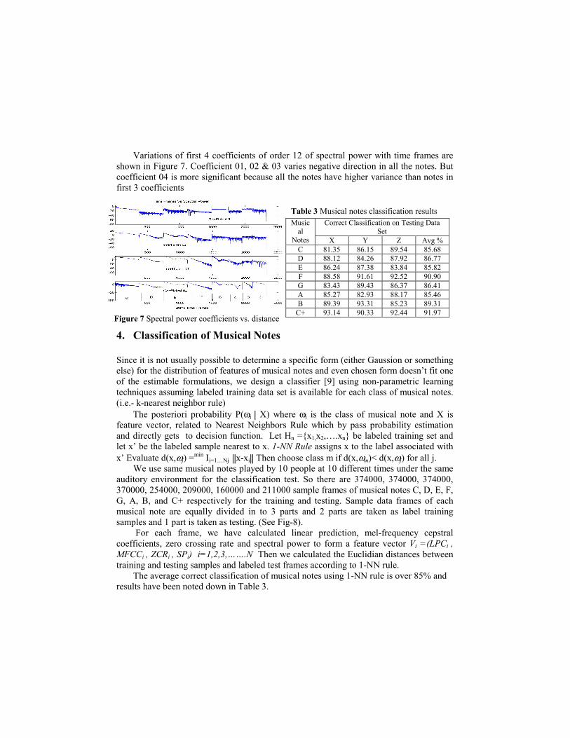
The rate at which zero crossing occurs is a simple measure of the frequency content of a signal. The number of zero crossing (number of times the sequence changes sign) is also a useful feature in music analysis.. Zero crossing rate is usually suitable for narrowband signals, but music signals include both narrowband and broadband components [11]. This feature is directly proportional to harmonic structure of the musical notes. It can be seen in Figure 6 that C and C+ have the lowest and highest average rates of zero crossing, because these notes have lowest and highest fundamental frequencies. The starting frames of all the note have high ZCR, because of the attacking time is nearly zero and just like impulse respond where frequency tends to infinity. Since note E and G have strong harmonics below the fundamental frequencies, they have comparatively lower average ZCR than note D and F.

3.7. Spectral Power (SP)

For a music signal )(ns , each frame is weighted with a Hamming window h(n), Where N is the number of samples of each frame. The spectral power of the signal )(ns is calculated according to equation (2). Since order 12 gives the maximum average distance [eqn (1) & Table 1] between musical notes (i.e 14.78) in the order range (2 to 25), we have used order 12 as the best spectral power order for our further experiments.

−= ∑

−

=

21

010 2exp()()(1log10)(

N

n Nnkjnhns

NkS π

(2)

Figure 6 Zero crossing rate vs. time frame

Figure 5 MFCC vs. time frames

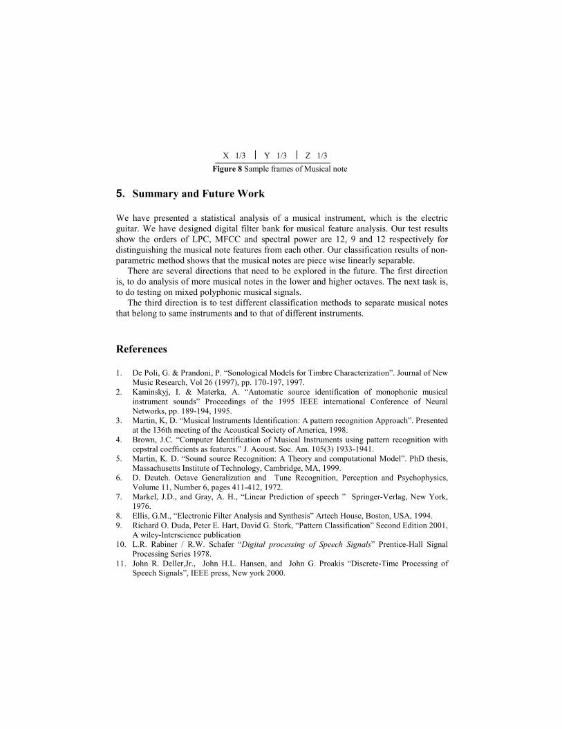
Variations of first 4 coefficients of order 12 of spectral power with time frames are

shown in Figure 7. Coefficient 01, 02 & 03 varies negative direction in all the notes. But coefficient 04 is more significant because all the notes have higher variance than notes in first 3 coefficients

4. Classification of Musical Notes

Since it is not usually possible to determine a specific form (either Gaussion or something else) for the distribution of features of musical notes and even chosen form doesn’t fit one of the estimable formulations, we design a classifier [9] using non-parametric learning techniques assuming labeled training data set is available for each class of musical notes. (i.e.- k-nearest neighbor rule)

The posteriori probability P(ωi | X) where ωi is the class of musical note and X is feature vector, related to Nearest Neighbors Rule which by pass probability estimation and directly gets to decision function. Let Hn =x1,x2,….xn be labeled training set and let x’ be the labeled sample nearest to x. 1-NN Rule assigns x to the label associated with x’ Evaluate d(x,ωj) =min Ii=1…Nj

||x-xi|| Then choose class m if d(x,ωm)< d(x,ωj) for all j. We use same musical notes played by 10 people at 10 different times under the same

auditory environment for the classification test. So there are 374000, 374000, 374000, 370000, 254000, 209000, 160000 and 211000 sample frames of musical notes C, D, E, F, G, A, B, and C+ respectively for the training and testing. Sample data frames of each musical note are equally divided in to 3 parts and 2 parts are taken as label training samples and 1 part is taken as testing. (See Fig-8).

For each frame, we have calculated linear prediction, mel-frequency cepstral coefficients, zero crossing rate and spectral power to form a feature vector Vi =(LPCi , MFCCi , ZCRi , SPi) i=1,2,3,…….N Then we calculated the Euclidian distances between training and testing samples and labeled test frames according to 1-NN rule.

The average correct classification of musical notes using 1-NN rule is over 85% and results have been noted down in Table 3.

Table 3 Musical notes classification results

Correct Classification on Testing Data Set

Musical

Notes X Y Z Avg % C 81.35 86.15 89.54 85.68 D 88.12 84.26 87.92 86.77 E 86.24 87.38 83.84 85.82 F 88.58 91.61 92.52 90.90 G 83.43 89.43 86.37 86.41 A 85.27 82.93 88.17 85.46 B 89.39 93.31 85.23 89.31

C+ 93.14 90.33 92.44 91.97 Figure 7 Spectral power coefficients vs. distance

5. Summary and Future Work

We have presented a statistical analysis of a musical instrument, which is the electric guitar. We have designed digital filter bank for musical feature analysis. Our test results show the orders of LPC, MFCC and spectral power are 12, 9 and 12 respectively for distinguishing the musical note features from each other. Our classification results of non-parametric method shows that the musical notes are piece wise linearly separable. There are several directions that need to be explored in the future. The first direction is, to do analysis of more musical notes in the lower and higher octaves. The next task is, to do testing on mixed polyphonic musical signals. The third direction is to test different classification methods to separate musical notes that belong to same instruments and to that of different instruments.

References

1. De Poli, G. & Prandoni, P. “Sonological Models for Timbre Characterization”. Journal of New Music Research, Vol 26 (1997), pp. 170-197, 1997.

2. Kaminskyj, I. & Materka, A. “Automatic source identification of monophonic musical instrument sounds” Proceedings of the 1995 IEEE international Conference of Neural Networks, pp. 189-194, 1995.

3. Martin, K, D. “Musical Instruments Identification: A pattern recognition Approach”. Presented at the 136th meeting of the Acoustical Society of America, 1998.

4. Brown, J.C. “Computer Identification of Musical Instruments using pattern recognition with cepstral coefficients as features.” J. Acoust. Soc. Am. 105(3) 1933-1941.

5. Martin, K. D. “Sound source Recognition: A Theory and computational Model”. PhD thesis, Massachusetts Institute of Technology, Cambridge, MA, 1999.

6. D. Deutch. Octave Generalization and Tune Recognition, Perception and Psychophysics, Volume 11, Number 6, pages 411-412, 1972.

7. Markel, J.D., and Gray, A. H., “Linear Prediction of speech ” Springer-Verlag, New York, 1976.

8. Ellis, G.M., “Electronic Filter Analysis and Synthesis” Artech House, Boston, USA, 1994. 9. Richard O. Duda, Peter E. Hart, David G. Stork, “Pattern Classification” Second Edition 2001,

A wiley-Interscience publication 10. L.R. Rabiner / R.W. Schafer “Digital processing of Speech Signals” Prentice-Hall Signal

Processing Series 1978. 11. John R. Deller,Jr., John H.L. Hansen, and John G. Proakis “Discrete-Time Processing of

Speech Signals”, IEEE press, New york 2000.

X 1/3 Z 1/3 Y 1/3Figure 8 Sample frames of Musical note