Embed Size (px)
Citation preview

Statistical Analysis of FamilialAggregation of Adverse Outcomes
Luise Cederkvist Kristiansen
Kongens Lyngby 2012IMM-MSc-2012-13

Technical University of DenmarkInformatics and Mathematical ModellingBuilding 321, DK-2800 Kongens Lyngby, DenmarkPhone +45 45253351, Fax +45 [email protected]
Summary
In survival analysis, the survival times of the subjects in the study population aregenerally assumed to be statistically independent, conditional on the covariateinformation. However, situations where the survival times are correlated due toa natural clustering of the study subjects may arise.
In this study, different statistical methods for analysis of clustered survival dataare evaluated and compared using data from a Danish register-based familystudy of the psychological effects of exposure to childhood cancer. In additionto assessing the effect of exposure to childhood cancer whilst coping with familialclustering, two of the presented models are applied in order to estimate familialcorrelation of ages at onset. The models show that individuals diagnosed withcancer and individuals with a family history of admission have an increasedhazard rate. Furthermore, a significant correlation of age at onset within familiesis identified.
Of the models presented, the shared gamma frailty Cox proportional hazardsmodel and the Clayton-Oakes copula model with the marginal Cox proportionalhazards model as margin are the most applicable in this study.

ii
Resume
I overlevelsesanalyse antages det generelt, at observationernes overlevelsestiderer statistisk uafhængige betinget af kovariaterne. Der kan imidlertid opsta si-tuationer, hvor overlevelsestiderne er korrelerede pga. en naturlig gruppering afdata.
I dette projekt evalueres og sammenlignes forskellige statistiske metoder til ana-lyse af korreleret overlevelsdata vha. data fra et dansk registerbaseret familie-studie af de psykologiske senfølger af eksponering for børnecancer. Udover atestimere effekten af eksponering for børnecancer, alt imens der tages højde for,at data er grupperet, kan to af de præsenterede modeller bruges til at estimerekorrelationen mellem overlevelsestiderne indenfor en familie. Modellerne viser,at individer, der diagnosticeres med kræft, samt individer med tidligere ind-læggelser i familien har en øget hazard rate. Endvidere ses det, at der er ensignifikant korrelation mellem overlevelsestiderne indenfor en familie.
De mest anvendelige modeller er i dette projekt shared gamma frailty Coxproportional hazards modellen og Clayton Oakes copula modellen med denmarginale Cox proportional hazards model som margin.

iv
Preface
This thesis was prepared at the Department of Informatics and MathematicalModelling (IMM), the Technical University of Denmark and at the Departmentof Statistics, Bioinformatics and Registry (SBR), the Danish Cancer Societyin partial fulfillment of the requirements for acquiring a Master of Science inEngineering. The thesis was supervised by Per Bruun Brockhoff, IMM, andco-supervised by Klaus Kaae Andersen and Kirsten Frederiksen, SBR.
The thesis deals with different statistical methods for analysis of clustered sur-vival data. The main focus is on semi-parametric methods, though also para-metric methods are presented. The statistical methods are explored using threesmall data sets and then applied to data from a Danish register-based familystudy of the psychological late effects of exposure to childhood cancer.
Copenhagen, February 2012
Luise Cederkvist Kristiansen

vi

Acknowledgements
First of all, I would like to thank my supervisors Per Bruun Brockhoff, KlausKaae Andersen and Kirsten Frederiksen. They have been great in different waysand have throughout this project offered valuable guidance and support. I havetruly appreciated my weekly meetings with Klaus and Kirsten, and I am gratefulof their commitment to my project.
I would also like to thank Lasse Wegener Lund from the Danish Cancer Societyfor letting me use his data in this study.
Finally, it would like to thank my parents for giving me shelter the last couple ofweekends and my friend Kathrine Grell for encouraging me and for proofreadingmy thesis.

viii
Contents
Summary i
Resume iii
Preface v
Acknowledgements vii
1 Introduction 1
1.1 Objectives . . . . . . . . . . . . . . . . . . . . . . . . . . . . . . . 2
1.2 Overview of thesis . . . . . . . . . . . . . . . . . . . . . . . . . . 3
2 Theory 5
2.1 Survival analysis . . . . . . . . . . . . . . . . . . . . . . . . . . . 5
2.1.1 Terminology . . . . . . . . . . . . . . . . . . . . . . . . . 6
2.2 Proportional hazards models . . . . . . . . . . . . . . . . . . . . 8
2.2.1 Weibull proportional hazards model . . . . . . . . . . . . 9
2.2.2 Cox proportional hazards model . . . . . . . . . . . . . . 11
2.2.3 Interpretation of the hazard ratio . . . . . . . . . . . . . . 12
2.2.4 Checking model assumptions . . . . . . . . . . . . . . . . 13
2.3 Analysis of clustered survival data . . . . . . . . . . . . . . . . . 15
2.3.1 Fixed effects model . . . . . . . . . . . . . . . . . . . . . . 15
2.3.2 Semi-parametric stratified model . . . . . . . . . . . . . . 16
2.3.3 Shared frailty model . . . . . . . . . . . . . . . . . . . . . 16
2.3.4 Marginal model . . . . . . . . . . . . . . . . . . . . . . . . 19
2.3.5 Copula model . . . . . . . . . . . . . . . . . . . . . . . . . 20
2.4 Measure of dependence . . . . . . . . . . . . . . . . . . . . . . . . 23
x CONTENTS
3 Materials & Methods 253.1 Data . . . . . . . . . . . . . . . . . . . . . . . . . . . . . . . . . . 25
3.1.1 Data sets available through R . . . . . . . . . . . . . . . . 263.1.2 Childhood cancer data . . . . . . . . . . . . . . . . . . . . 31
3.2 Statistical analysis . . . . . . . . . . . . . . . . . . . . . . . . . . 35
4 Results 374.1 Data sets available through R . . . . . . . . . . . . . . . . . . . . 37
4.1.1 Diabetic retinopathy data . . . . . . . . . . . . . . . . . . 374.1.2 Kidney catheter data . . . . . . . . . . . . . . . . . . . . . 444.1.3 NCCTG lung cancer data . . . . . . . . . . . . . . . . . . 50
4.2 Childhood cancer data . . . . . . . . . . . . . . . . . . . . . . . . 574.2.1 Unadjusted Cox proportional hazards model . . . . . . . 574.2.2 Shared gamma frailty Cox proportional hazards model . . 584.2.3 Clayton-Oakes copula model . . . . . . . . . . . . . . . . 614.2.4 Summary of results . . . . . . . . . . . . . . . . . . . . . . 63
5 Discussion 655.1 Data sets available through R . . . . . . . . . . . . . . . . . . . . 655.2 Childhood cancer data . . . . . . . . . . . . . . . . . . . . . . . . 67
5.2.1 Degree of dependence . . . . . . . . . . . . . . . . . . . . 675.2.2 Robust standard errors . . . . . . . . . . . . . . . . . . . 67
5.3 Discussion of models . . . . . . . . . . . . . . . . . . . . . . . . . 695.4 Checking the adequacy of the model . . . . . . . . . . . . . . . . 705.5 Extensions . . . . . . . . . . . . . . . . . . . . . . . . . . . . . . . 71
6 Conclusion 73
A R Code 75A.1 R code for data examples . . . . . . . . . . . . . . . . . . . . . . 75A.2 R code for childhood cancer data . . . . . . . . . . . . . . . . . . 81
B Additional Results 85B.1 Kidney catheter data . . . . . . . . . . . . . . . . . . . . . . . . . 85
Bibliography 87
List of Tables
3.1 Diabetic retinopathy data: Incidence rates by treatment groupand disease onset . . . . . . . . . . . . . . . . . . . . . . . . . . . 26
3.2 Kidney catheter data: Incidence rates by gender . . . . . . . . . 28
3.3 Kidney catheter data: Incidence rates by age group . . . . . . . . 28
3.4 NCCTG lung cancer data: Incidence rates by gender . . . . . . . 29
3.5 NCCTG lung cancer data: Incidence rates by age group . . . . . 29
3.6 NCCTG lung cancer data: Incidence rates by ECOG score . . . 31
3.7 Childhood cancer data: Distribution of individuals . . . . . . . . 32
3.8 Childhood cancer data: Number of family members . . . . . . . . 32
3.9 Childhood cancer data: Distribution of number of events . . . . . 33
3.10 Childhood cancer data: Incidence rates by exposure groups . . . 34
3.11 Childhood cancer data: Incidence rates by previous admission . . 34
4.1 Diabetic retinopathy data: Estimates from unadjusted model . . 38
xii LIST OF TABLES
4.2 Diabetic retinopathy data: Hazard ratios from unadjusted model 38
4.3 Diabetic retinopathy data: Estimates from stratified model . . . 39
4.4 Diabetic retinopathy data: Estimates from shared frailty model . 40
4.5 Diabetic retinopathy data: Hazard ratios from shared frailty model 40
4.6 Diabetic retinopathy data: Estimates from copula model . . . . . 42
4.7 Diabetic retinopathy data: Hazard ratios from copula model . . . 42
4.8 Diabetic retinopathy data: Summary of results . . . . . . . . . . 43
4.9 Kidney catheter data: Estimates from unadjusted model . . . . . 44
4.10 Kidney catheter data: Estimates from shared frailty model . . . 46
4.11 Kidney catheter data: Estimates from copula model . . . . . . . 47
4.12 Kidney catheter data: Summary of results . . . . . . . . . . . . . 49
4.13 NCCTG lung cancer data: Estimates from unadjusted model . . 50
4.14 NCCTG lung cancer data: Estimates from fixed effects model . . 52
4.15 NCCTG lung cancer data: Estimates from stratified model . . . 53
4.16 NCCTG lung cancer data: Estimates from shared frailty model . 54
4.17 NCCTG lung cancer data: Estimates from copula model . . . . . 55
4.18 NCCTG lung cancer data: Summary of results . . . . . . . . . . 56
4.19 Childhood cancer data: Estimates from unadjusted model . . . . 57
4.20 Childhood cancer data: Hazard ratios from unadjusted model . . 58
4.21 Childhood cancer data: Estimates from shared frailty model . . . 59
4.22 Childhood cancer data: Hazard ratios from shared frailty model . 59
4.23 Childhood cancer data: Estimates from copula model . . . . . . 62
LIST OF TABLES xiii
4.24 Childhood cancer data: Hazard ratios from copula model . . . . 62
4.25 Childhood cancer data: Summary of results . . . . . . . . . . . . 64
5.1 Childhood cancer data: Estimates from marginal model fittedusing the function cox.aalen . . . . . . . . . . . . . . . . . . . . 68
5.2 Childhood cancer data: Estimates from marginal model fittedusing the function coxph . . . . . . . . . . . . . . . . . . . . . . . 68
5.3 Childhood cancer data: Estimates from marginal model fittedusing the function cox.aalen . . . . . . . . . . . . . . . . . . . . 69
5.4 Childhood cancer data: Estimates from marginal model fittedusing the function coxph . . . . . . . . . . . . . . . . . . . . . . . 69
B.1 Kidney catheter data: Additional results . . . . . . . . . . . . . . 86
xiv LIST OF TABLES
List of Figures
2.1 An example of survival times and censoring. . . . . . . . . . . . . 7
2.2 An example of a hypothetical survival function. . . . . . . . . . . 8
2.3 Hazard functions for Weibull distributed survival times. . . . . . 10
3.1 Diabetic retinopathy data: Cumulative incidence for treatmentgroup and disease onset . . . . . . . . . . . . . . . . . . . . . . . 27
3.2 Kidney catheter data: Cumulative incidence for gender . . . . . . 28
3.3 NCCTG lung cancer data: Distribution of patients . . . . . . . . 30
3.4 NCCTG lung cancer data: Cumulative incidence for gender . . . 30
3.5 Childhood cancer data: Cumulative incidence for exposure group 33
3.6 Childhood cancer data: Cumulative incidence for previous ad-mission . . . . . . . . . . . . . . . . . . . . . . . . . . . . . . . . 34
4.1 Diabetic retinopathy data: Visualisation of results . . . . . . . . 39
4.2 Diabetic retinopathy data: Histogram of frailties . . . . . . . . . 41
xvi LIST OF FIGURES
4.3 Kidney catheter data: Relationship between age and incidencerecurrent infection . . . . . . . . . . . . . . . . . . . . . . . . . . 45
4.4 Kidney catheter data: Histogram of frailties . . . . . . . . . . . . 46
4.5 NCCTG lung cancer data: Relationship between age and inci-dence death . . . . . . . . . . . . . . . . . . . . . . . . . . . . . . 51
4.6 NCCTG lung cancer data: Relationship between ECOG scoreand incidence death . . . . . . . . . . . . . . . . . . . . . . . . . 51
4.7 NCCTG lung cancer data: Histogram of frailties . . . . . . . . . 54
4.8 Childhood cancer data: Visualisation of results 1 . . . . . . . . . 58
4.9 Childhood cancer data: Visualisation of results 2 . . . . . . . . . 60
4.10 Childhood cancer data: Histogram of frailties . . . . . . . . . . . 60
4.11 Childhood cancer data: Frailties and number of events . . . . . . 61
4.12 Childhood cancer data: Visualisation of results 3 . . . . . . . . . 63
Chapter 1
Introduction
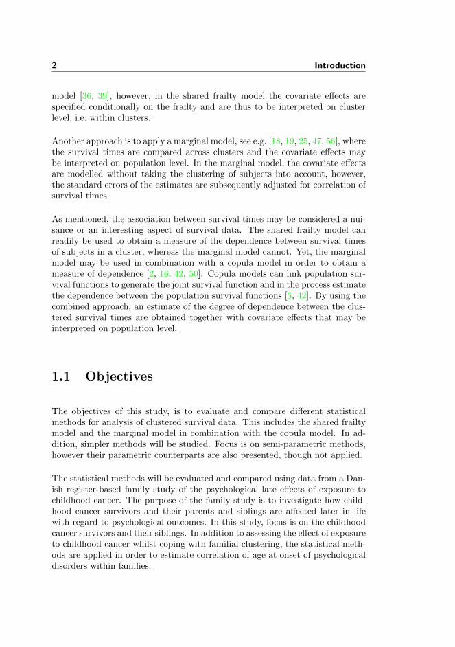
In survival analysis, the survival times of the subjects in the study population aregenerally assumed to be statistically independent, conditional on the covariateinformation. However, situations where the survival times are correlated due toa natural clustering of the study subjects may arise and can occur for differentkinds of data [23, 36]. Simple examples where independence between survivaltimes cannot be assumed are the lifetimes of related individuals, e.g. twins, ortime between recurrent events.
Dependence between survival times may be considered a nuisance of survivaldata. In other applications the correlation is of primary interest. For example,in family studies, correlation of age at onset is typically of main interest andconsidered as evidence of familial aggregation [1]. Familial aggregation may beattributed to unobserved genetic and environmental factors, which are sharedby the members of a family, and it may be important for understanding theetiology of many common diseases including cancers and psychiatric disorders.
A commonly used and very general approach to the modelling of clustered sur-vival data is to assume that there is an unobserved risk factor, a so-called frailty,which is shared by all subjects in a cluster, see e.g. [22, 24, 35, 37, 43, 49]. This issimilar to classic linear regression, where a cluster effect is typically modelled asa random effect. In the classic linear regression model, the mean of the responsevariable is unaltered by the random effect because of the linear structure of the
2 Introduction
model [36, 39], however, in the shared frailty model the covariate effects arespecified conditionally on the frailty and are thus to be interpreted on clusterlevel, i.e. within clusters.
Another approach is to apply a marginal model, see e.g. [18, 19, 25, 47, 56], wherethe survival times are compared across clusters and the covariate effects maybe interpreted on population level. In the marginal model, the covariate effectsare modelled without taking the clustering of subjects into account, however,the standard errors of the estimates are subsequently adjusted for correlation ofsurvival times.
As mentioned, the association between survival times may be considered a nui-sance or an interesting aspect of survival data. The shared frailty model canreadily be used to obtain a measure of the dependence between survival timesof subjects in a cluster, whereas the marginal model cannot. Yet, the marginalmodel may be used in combination with a copula model in order to obtain ameasure of dependence [2, 16, 42, 50]. Copula models can link population sur-vival functions to generate the joint survival function and in the process estimatethe dependence between the population survival functions [5, 42]. By using thecombined approach, an estimate of the degree of dependence between the clus-tered survival times are obtained together with covariate effects that may beinterpreted on population level.
1.1 Objectives
The objectives of this study, is to evaluate and compare different statisticalmethods for analysis of clustered survival data. This includes the shared frailtymodel and the marginal model in combination with the copula model. In ad-dition, simpler methods will be studied. Focus is on semi-parametric methods,however their parametric counterparts are also presented, though not applied.
The statistical methods will be evaluated and compared using data from a Dan-ish register-based family study of the psychological late effects of exposure tochildhood cancer. The purpose of the family study is to investigate how child-hood cancer survivors and their parents and siblings are affected later in lifewith regard to psychological outcomes. In this study, focus is on the childhoodcancer survivors and their siblings. In addition to assessing the effect of exposureto childhood cancer whilst coping with familial clustering, the statistical meth-ods are applied in order to estimate correlation of age at onset of psychologicaldisorders within families.
1.2 Overview of thesis 3
Before the statistical methods are applied to the large data set from the register-based family study, they are explored using three smaller data sets, which areavailable through the statistical software R [48].
1.2 Overview of thesis
Chapter 2 will start with a brief introduction to survival analysis, where thebasic terminology will be covered. Hereafter, the different statistical methods,which are applied in this study, will be presented. Although, focus in this studyis on semi-parametric survival models, their parametric counterparts are alsopresented. In Chapter 3, the data analysed in this study will be presented andit will be described how the statistical analyses are conducted. The results fromthe statistical analyses are presented in Chapter 4. In Chapter 5, the appliedstatistical models are discussed based on the results. This will be followed bysuggestions for further work. Finally, a summary of the results and conclusionsis given in Chapter 6.
4 Introduction
Chapter 2
Theory
In this chapter, the different statistical methods, which are applied in this study,will be described. First, a brief introduction to survival analysis is given andthen the proportional hazards model is presented. Finally, different statisticalmethods for analysis of clustered survival data are presented. The methods areall based on the proportional hazards model. Two of the methods presented,may be applied for estimation of the degree of dependence between the clusteredsurvival data.
2.1 Survival analysis
Survival analysis is statistical analysis of data, where the response of interest istime from a well-defined origin to the occurrence of an event of interest [36]. Akey feature, which makes survival analysis different from other areas in statisticsis that survival data is usually censored [7]. Censoring occurs when the exactsurvival time (time until event of interest) is unknown. The survival time maybe unknown because the subjects have withdrawn from the study or in someother way been lost to follow-up, e.g. moved to another country. For thesesubjects, the survival time is at least until withdrawal or last contact. Subjectsfor whom no event of interest has occurred at the end of the study are also
6 Theory
censored. Their survival times are at least until the end of the study. The typeof censoring described here is called right censoring and is the most commonform of censoring in survival data [27] though other censoring schemes exist,e.g. left censoring which is applied when the event of interest occurs prior to acertain time t or interval censoring which is applied if the event of interest occursbetween times ta and tb. Censoring is assumed to be statistically independentof the survival time.
In addition to censoring, survival data can be truncated. Truncation is con-cerned with the entry of subjects into a study. When the survival data is trun-cated, only subjects with survival times within a certain interval, e.g. [TL, TR]are observed. Left truncation occurs when subjects for whom the event of in-terest either has occurred before some truncation threshold TL, i.e. T < TL, oris known never to occur, are excluded from the study. Right truncation occurwhen subjects for whom the event of interest has occurred after some truncationthreshold TR, i.e. TR < T , are excluded from the study [29].
2.1.1 Terminology
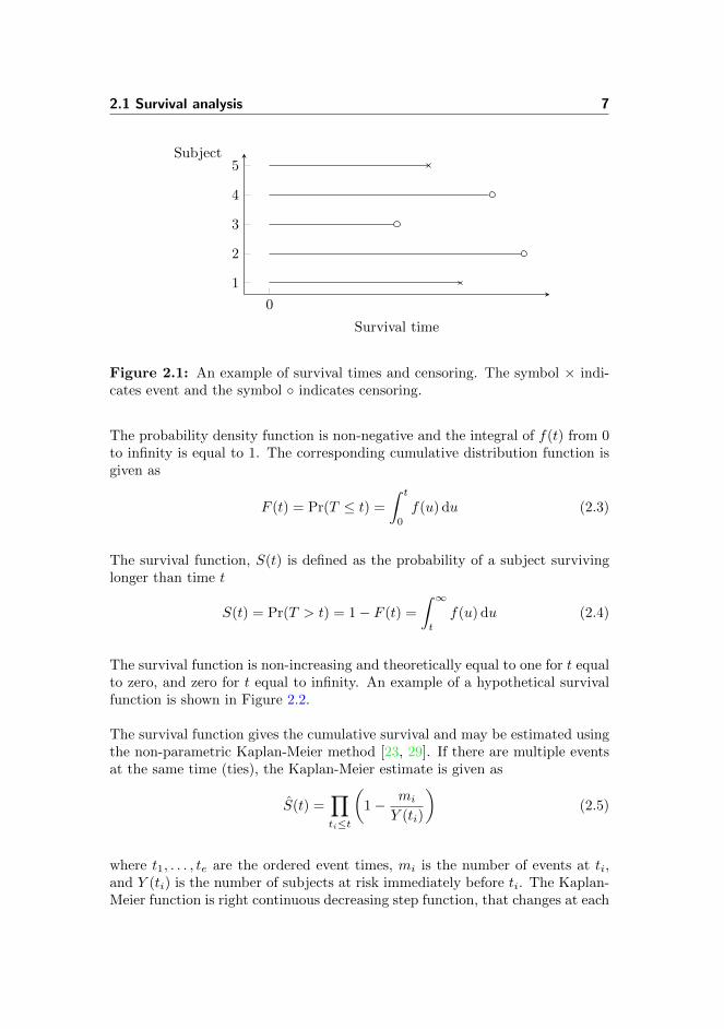
The information of interest for a subject is contained in the pair (T, δ), where Tis the survival time until the event of interest or censoring, and δ is the censoringindicator. The survival time T is a random variable and is equal to or greaterthan 0. The indicator variable δ is equal to 1 if the event of interest has occurredand 0 otherwise
T ≥ 0 and δ =
{1 if event0 if censored
A visualisation of (T, δ) is given in Figure 2.1.
Three important and closely related functions in survival analysis are the proba-bility density function, f(t), the survival function, S(t), and the hazard function,h(t). Specifying one of three functions, specifies all three functions as there is aclearly defined relationship between them, i.e. the probability density functioncan be expressed as
f(t) = h(t)S(t) (2.1)
The probability density function, f(t), gives the unconditional event rate and isdefined as
f(t) = lim∆t→0
Pr(t ≤ T < t+ ∆t)
∆t(2.2)
2.1 Survival analysis 7
0
1
2
3
4
5
Survival time
Subject
Figure 2.1: An example of survival times and censoring. The symbol × indi-cates event and the symbol ◦ indicates censoring.
The probability density function is non-negative and the integral of f(t) from 0to infinity is equal to 1. The corresponding cumulative distribution function isgiven as
F (t) = Pr(T ≤ t) =
∫ t
0
f(u) du (2.3)
The survival function, S(t) is defined as the probability of a subject survivinglonger than time t
S(t) = Pr(T > t) = 1− F (t) =
∫ ∞t
f(u) du (2.4)
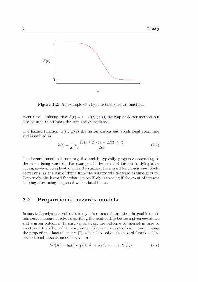
The survival function is non-increasing and theoretically equal to one for t equalto zero, and zero for t equal to infinity. An example of a hypothetical survivalfunction is shown in Figure 2.2.
The survival function gives the cumulative survival and may be estimated usingthe non-parametric Kaplan-Meier method [23, 29]. If there are multiple eventsat the same time (ties), the Kaplan-Meier estimate is given as
S(t) =∏ti≤t
(1− mi
Y (ti)
)(2.5)
where t1, . . . , te are the ordered event times, mi is the number of events at ti,and Y (ti) is the number of subjects at risk immediately before ti. The Kaplan-Meier function is right continuous decreasing step function, that changes at each
8 Theory
0
1
t
S(t)
Figure 2.2: An example of a hypothetical survival function.
event time. Utilising, that S(t) = 1−F (t) (2.4), the Kaplan-Meier method canalso be used to estimate the cumulative incidence.
The hazard function, h(t), gives the instantaneous and conditional event rateand is defined as
h(t) = lim∆t→0
Pr(t ≤ T < t+ ∆t|T ≥ t)∆t
(2.6)
The hazard function is non-negative and it typically progresses according tothe event being studied. For example, if the event of interest is dying afterhaving received complicated and risky surgery, the hazard function is most likelydecreasing, as the risk of dying from the surgery will decrease as time goes by.Conversely, the hazard function is most likely increasing if the event of interestis dying after being diagnosed with a fatal illness.
2.2 Proportional hazards models
In survival analysis as well as in many other areas of statistics, the goal is to ob-tain some measure of effect describing the relationship between given covariatesand a given outcome. In survival analysis, the outcome of interest is time toevent, and the effect of the covariates of interest is most often measured usingthe proportional hazards model [7], which is based on the hazard function. Theproportional hazards model is given as
h(t|X) = h0(t) exp(X1β1 +X2β2 + . . .+Xkβk) (2.7)
2.2 Proportional hazards models 9
where h0(t) is the baseline hazard function, X1, . . . , Xk are the covariates, andβ1, . . . , βk are the covariate effects. The covariate effects act multiplicatively onand thereby scale the baseline hazard function, which is common to all subjects.As seen, the effects of the covariates are independent of time, and thus assumedto be the same at all values of t. The covariate effects are additive and linearfor the log hazard
log(h(t|X)) = log(h0(t)) +X1β1 +X2β2 + . . .+Xkβk (2.8)
The baseline hazard function h0(t) can be assumed to have a particular paramet-ric form, i.e. have the survival times follow some distribution, or left unspecified.Commonly used distributions for the survival times are the Weibull distribution,the exponential distribution (which is a special case of the Weibull distribution),and the log-logistic distribution [27]. If the baseline hazard is left unspecified,the proportional hazards model is semi-parametric. In the following sections,the parametric Weibull proportional hazards model and the semi-parametricCox proportional hazards model are introduced.
2.2.1 Weibull proportional hazards model
The Weibull model is the most widely used parametric survival model [27]. Ifthe survival times are assumed to be Weibull distributed, T ∼ W (λ, ρ), thenthe hazard function is given as
h(t) = λρtρ−1, ρ > 0 and λ > 0 (2.9)
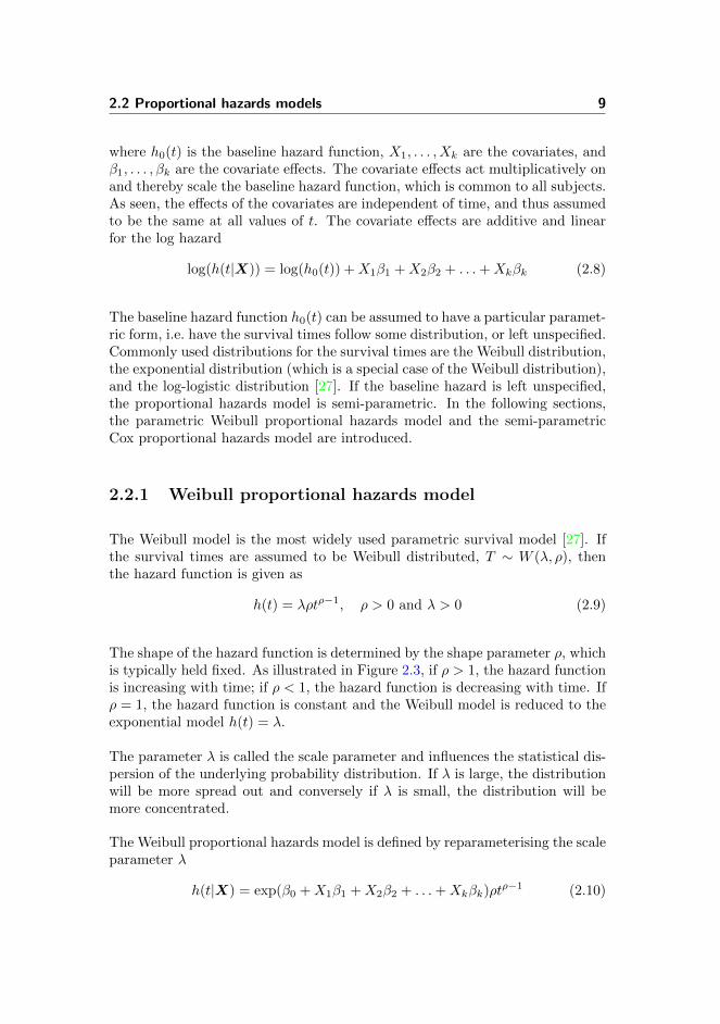
The shape of the hazard function is determined by the shape parameter ρ, whichis typically held fixed. As illustrated in Figure 2.3, if ρ > 1, the hazard functionis increasing with time; if ρ < 1, the hazard function is decreasing with time. Ifρ = 1, the hazard function is constant and the Weibull model is reduced to theexponential model h(t) = λ.
The parameter λ is called the scale parameter and influences the statistical dis-persion of the underlying probability distribution. If λ is large, the distributionwill be more spread out and conversely if λ is small, the distribution will bemore concentrated.
The Weibull proportional hazards model is defined by reparameterising the scaleparameter λ
h(t|X) = exp(β0 +X1β1 +X2β2 + . . .+Xkβk)ρtρ−1 (2.10)
10 Theory
0 0.2 0.4 0.6 0.8 1
0
2
4
6
8
Time
Haza
rdfu
nct
ion
ρ = 0.2ρ = 1ρ = 5
Figure 2.3: Hazard functions for Weibull distributed survival times. Hazardfunctions with different values for ρ are depicted with λ = 1.
The Weibull proportional hazards model can also be expressed as in (2.7)
h(t|X) = exp(β0)ρtρ−1 exp(X1β1 +X2β2 + . . .+Xkβk) (2.11)
where exp(β0)ρtρ−1 may be regarded as h0(t).
2.2.1.1 Estimation of the Weibull proportional hazards model
As the Weibull proportional hazards model is fully parametric, the model pa-rameters are estimated by maximising the likelihood function. Right censoredsurvival data consists of a combination of subjects that experience an event andsubjects that are right censored, and as a result [7], the likelihood function fora sample with n subjects is given by
Ln(α|T , δ) =
n∏i=1
(f(Ti))δi(S(Ti))
1−δi (2.12)
whereα is the parameter vector of interest. Utilising that the probability densityfunction, f(t), can be expressed as a product of the survival function and thehazard function (2.1), the likelihood function can be rewritten as
Ln(α|T , δ) =
n∏i=1
(h(Ti))δiS(Ti) (2.13)

2.2 Proportional hazards models 11
For Weibull distributed event times, the likelihood function is
Ln(β, ρ|T , δ,X) =
n∏i=1
(ρT ρ−1i exp(Xiβ))δi exp(−T ρi exp(Xiβ)) (2.14)
where Xi = (1, Xi1, . . . , Xik) and β = (β0, β1, . . . , βk)T . The log-likelihoodfunction `n(α) = logLn(α), is typically easier to work with than the likelihoodfunction itself, and it is therefore used in the maximisation process. It makes nodifference since maximising the log-likelihood gives the same estimates as max-imising the likelihood. The log-likelihood function is maximised in an iterativelymanner.
2.2.2 Cox proportional hazards model
The baseline hazard function in the proportional hazards model (2.7) can be leftunspecified, which will result in a semi-parametric proportional hazards model.The most widely used semi-parametric survival model is the Cox proportionalhazards model, which is given as
h(t|X) = h0(t) exp(X1β1 +X2β2 + . . .+Xkβk) (2.15)
The model is semi-parametric, because while no knowledge of the baseline haz-ard function, h0(t), is required, the covariates still enter the model linearly onthe log hazard scale.
2.2.2.1 Estimation of the Cox proportional hazards model
Since the Cox proportional hazards model is semi-parametric, the model pa-rameters cannot be estimated using the likelihood function in (2.13). Instead,one must use the method of partial likelihood, developed by David R. Cox in1972 [6]. The partial likelihood function is given by
Ln(β|X, T ) =
r∏i=1
exp(Xiβ)∑Tj≥Ti exp(Xjβ)
(2.16)
where r is the number of events, Xi = (Xi1, . . . , Xik), and Xj = (Xj1, . . . , Xjk).The likelihood is called partial, as only the probabilities of subjects that ex-perience an event are considered [27]. The estimates obtained by the partial
12 Theory
likelihood are consistent and asymptotic normal [9, 12], and found by maximis-ing the partial log-likelihood in an iteratively manner. The partial likelihood isvalid when no subjects have the same event time (no ties). If this is not thecase, the Efron approximation [8, 52] to the partial likelihood may be applied.
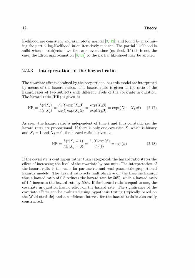
2.2.3 Interpretation of the hazard ratio
The covariate effects obtained by the proportional hazards model are interpretedby means of the hazard ratios. The hazard ratio is given as the ratio of thehazard rates of two subjects with different levels of the covariate in question.The hazard ratio (HR) is given as
HR =h(t|Xi)
h(t|Xj)=h0(t) exp(Xiβ)
h0(t) exp(Xjβ)=
exp(Xiβ)
exp(Xjβ)= exp((Xi −Xj)β) (2.17)
As seen, the hazard ratio is independent of time t and thus constant, i.e. thehazard rates are proportional. If there is only one covariate X, which is binaryand Xi = 1 and Xj = 0, the hazard ratio is given as
HR =h(t|Xi = 1)
h(t|Xj = 0)=h0(t) exp(β)
h0(t)= exp(β) (2.18)
If the covariate is continuous rather than categorical, the hazard ratio states theeffect of increasing the level of the covariate by one unit. The interpretation ofthe hazard ratio is the same for parametric and semi-parametric proportionalhazards models. The hazard ratio acts multiplicative on the baseline hazard,thus a hazard ratio of 0.5 reduces the hazard rate by 50%, while a hazard ratioof 1.5 increases the hazard rate by 50%. If the hazard ratio is equal to one, thecovariate in question has no effect on the hazard rate. The significance of thecovariate effects can be evaluated using hypothesis testing (typically based onthe Wald statistic) and a confidence interval for the hazard ratio is also easilyconstructed.
2.2 Proportional hazards models 13
2.2.4 Checking model assumptions
A key assumption of the proportional hazards model is proportional hazards,which means that the hazard ratio of two subjects is constant and the covariateeffects are independent of time. The appropriateness of the proportional hazardsassumption may be evaluated using different approaches:
• Log-log survival curves
• Checking the Scoenfeld residuals
• Interaction of covariates with time
Log-log survival curves It can be shown that
S(t) = exp(−∫ t
0
h(u|X) du)
= exp(−∫ t
0
h0(u) exp(Xβ) du)
(2.19)
= exp(−H0(t) exp(Xβ))
where H0(t) =∫ t
0h0(u) du. In consequence
log(S(t)) = −H0(t) exp(Xβ) ⇔log(− log(S(t))) = log(−H0(t)) +Xβ (2.20)
Thus, the proportional hazards assumption may be evaluated by visualising thelog-log survival curves of the different levels of the covariates. The survivalcurves may be estimated using the non-parametric Kaplan-Meier method [23,29]. If the covariates are continuous, they will need to be categorised into anappropriate number of groups. If the log-log survival curves are approximatelyparallel when plotted on the log-log scale, the proportional hazards assumptionis satisfied.
Checking the Schoenfeld residuals Another way of checking the propor-tional hazards assumption is by means of the scaled Schoenfeld residuals. Itcan be shown, that if the proportional hazards assumption for a given covariateholds, then the Schoenfeld residuals for that covariate will be independent ofthe survival time. The method is elaborated by Therneau and Grambsch in [20]and [52].
14 Theory
Interaction of covariates with time The proportional hazards assumptioncan also be evaluated by extending the proportional hazards model and includingan interaction term involving the covariate being assessed and some function oftime [27]. The proportional hazards assumption is then evaluated by testingthe significance of the interaction term. The significance may be tested using aWald test or a likelihood ratio test.
Weibull assumption
In addition to the proportional hazards assumption, the Weibull proportionalhazards model is based on the assumption that the survival times are Weibulldistributed. This assumption can also be evaluated by means of the log-logsurvival curves. The Weibull survival function is given by
S(t) = exp(−λtρ) (2.21)
And thus
log(− log(S(t))) = log(λ) + ρ log(t) (2.22)
From (2.22), it is seen that the log(− log(S(t))) is a linear function of log(t). Thismeans, that if the log-log survival curves are reasonably straight, the Weibullassumption holds. If the log-log survival curves are parallel but not straight, itmeans the proportional hazards assumption holds, but the Weibull assumptiondoes not and vice versa. If the Weibull assumption holds and the proportionalhazards assumption does not, this indicates that the shape parameter ρ cannotassumed to be constant in the Weibull proportional hazards model (2.10)[27].In Kleinbaum and Klein (2005) a method for modeling ρ is presented.
Linearity of continuous covariates
The linearity of continuous covariates may be checked by visual inspection ofthe exposure-response relationship between the covariate in question and the logrelative hazard or by adding higher-order terms of the covariate and checkingtheir significance. Furthermore, the linearity may be checked by comparing themodel fit to that of a more flexible model, e.g. a spline model [52].
2.3 Analysis of clustered survival data 15
2.3 Analysis of clustered survival data
In the following sections, different statistical methods for analysis of clusteredsurvival data are presented. Only methods based on the proportional hazardsmodel will be considered. First, the fixed effects model and the semi-parametricstratified model will be presented. The two methods are computationally simple,but have some major drawbacks [7]. Then, the shared frailty model will be pre-sented. In the shared frailty model all subjects in a cluster are assumed to sharea random cluster effect, which impacts the interpretation of the hazard ratio.Finally, the marginal model and the copula model are presented. The marginalmodel is an independence working model, which means that the estimates areobtained by assuming all subjects are independent. The estimated parametervariance of the estimates are subsequently adjusted according to the correlationbetween subjects. The copula model can be used to combine the marginal sur-vival functions of different subjects in a cluster and thereby generate the jointsurvival function.
2.3.1 Fixed effects model
The clustering of data may be modeled by introducing a fixed effect for eachcluster in the proportional hazards model
hij(t|Xij) = h0(t) exp(Xijβ + ci) (2.23)
where hij(t) is the conditional hazard function for subject j in cluster i, ci isthe fixed effect for cluster i, and Xij = (Xij1, . . . , Xijk). The introduction ofa fixed cluster effect results in a loss of degrees of freedom, and to avoid anoverparameterised model, a restriction is necessary, e.g. c1 = 0. As a result,the fixed effects of all other clusters are to be compared to cluster 1, whichcomplicates the model interpretation. In addition, since the number of subjectsin each cluster is likely to be limited, the standard errors of the fixed effects willbe very large. Moreover, there may be some clusters with no events and onlycensored observations, where the hazard is difficult to estimate [7]. However,the fixed effect estimates and their standard errors are of secondary interest,as the fixed effect is introduced in order to adjust for the clustering and not toestimate the fixed cluster effects per se.

16 Theory
2.3.2 Semi-parametric stratified model
In the semi-parametric stratified model, each cluster is allowed to have its ownunspecified baseline hazard
hij(t|Xij) = hi0(t) exp(Xijβ) (2.24)
where hij(t) is the conditional hazard function for subject j in cluster i, hi0is the baseline hazard for cluster i, and Xij = (Xij1, . . . , Xijk). The partiallikelihood function for the stratified model is
Ln(β|X,T , δ) =
s∏i=1
ni∏j=1
(exp(Xijβ)∑
Til≥Tij exp(Xilβ)
)δij(2.25)
where s is the number of clusters, ni is the number of subjects in the ith cluster.A cluster only contributes to the partial likelihood if an event for a subject occurswhile at least one other subject is still at risk. Furthermore, a cluster where allsubjects have the same covariate information do not contribute to the partiallikelihood [7, 23].
2.3.3 Shared frailty model
Another way of managing clustering of data is by assuming that there is anunobserved risk factor, a so-called frailty, which is shared by all subjects in acluster. The frailty accounts for the between-group variability and simultane-ously induces a dependence within clusters [23]. The shared frailty model isdefined as
hij(t|Xij) = h0(t)ui exp(Xijβ) (2.26)
where hij(t|Xij) is the conditional hazard function for subject j in cluster i,and ui is the frailty of cluster i. The frailty is considered random and constantover time and acts multiplicatively on the baseline hazard function. Given thevalues of the frailties, the subjects are assumed to be independent, thus theshared frailty model is a conditional independence model [23]. The frailty israndom, because focus is not on each cluster as such, but on the population ofclusters [23].
2.3 Analysis of clustered survival data 17
2.3.3.1 Choice of frailty distribution
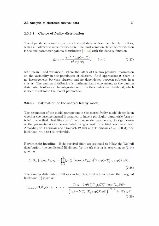
The dependence structure in the clustered data is described by the frailties,which all follow the same distribution. The most common choice of distributionis the one-parameter gamma distribution [7, 23] with the density function
fU (u) =u1/θ−1 exp(−u/θ)
θ1θ Γ(1/θ)
, θ > 0 (2.27)
with mean 1 and variance θ, where the latter of the two provides informationon the variability in the population of clusters. As θ approaches 0, there isno heterogeneity between clusters and no dependence between subjects in acluster. The gamma distribution is mathematically convenient, as the gammadistributed frailties can be integrated out from the conditional likelihood, whichis used to estimate the model parameters.
2.3.3.2 Estimation of the shared frailty model
The estimation of the model parameters in the shared frailty model depends onwhether the baseline hazard is assumed to have a particular parametric form oris left unspecified. Just like any of the other model parameters, the significanceof the parameter θ can be evaluated using a Wald or a likelihood ratio test.According to Therneau and Gramsch (2000) and Therneau et al. (2003), thelikelihood ratio test is preferable.
Parametric baseline If the survival times are assumed to follow the Weibulldistribution, the conditional likelihood for the ith cluster is according to (2.14)given as
Li(β, ρ|Ti, δi, Xi, ui) =
ni∏j=1
(ρT ρ−1ij ui exp(Xijβ))δij exp(−T ρijui exp(Xijβ))
(2.28)
The gamma distributed frailties can be integrated out to obtain the marginallikelihood [7] given as
Lmarg,i(β, θ, ρ|Ti, δi, Xi, ei) =Γ(ei + 1/θ)
∏nij=1(ρT ρ−1
ij exp(Xijβ))δij(1/θ +
∑nij=1 T
ρij exp(Xijβ)
)1/θ+diθ1/θΓ(1/θ)
(2.29)
18 Theory
where ei is the number of events in the ith cluster. By taking the logarithmof this expression and summing over all clusters, the marginal log-likelihoodfunction is obtained [7], and the model parameters can be estimated by max-imisation.
Unspecified baseline If the shared frailty model is semi-parametric andbased on the Cox proportional hazards model, the model parameters can be esti-mated using either partial likelihood ideas in combination with the expectation-maximisation (EM) algorithm [26] or the penalised partial likelihood. If thefrailties follow a gamma distribution, the two approaches lead to the same so-lution [7, 52, 53]. In this study, focus is on the penalised partial likelihoodapproach, which is implemented in the R function coxph.
The penalised partial log-likelihood function can be written as a sum of twoparts
`ppl(ζ,u) = `part(β,u) + `pen(u) (2.30)
where ζ = (β, θ), and
`part(β,u) = log
s∏i=1
ni∏j=1
(ui exp(Xijβ)∑
Tqw>Tijuq exp(Xqwβ)
)δij(2.31)
and
`pen(u) =
s∑i=1
log fU (ui) (2.32)
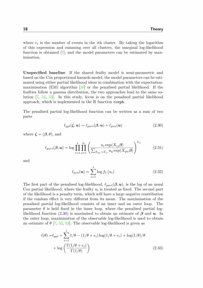
The first part of the penalised log-likelihood, `part(β,u), is the log of an usualCox partial likelihood, where the frailty ui is treated as fixed. The second partof the likelihood is a penalty term, which will have a large negative contributionif the random effect is very different from its mean. The maximisation of thepenalised partial log-likelihood consists of an inner and an outer loop. Theparameter θ is held fixed in the inner loop, where the penalised partial log-likelihood function (2.30) is maximised to obtain an estimate of β and u. Inthe outer loop, maximisation of the observable log-likelihood is used to obtainan estimate of θ [7, 52, 53]. The observable log-likelihood is given as
`(θ) =`ppl +
s∑i=1
1/θ − (1/θ + ei) log(1/θ + ei) + log(1/θ)/θ
+ log
(Γ(1/θ + ei)
Γ(1/θ)
)(2.33)
2.3 Analysis of clustered survival data 19
where ei is the number of events in the ith cluster. The maximisation process isconducted in an iteratively manner and can be quite computationally expensiveand time-consuming [53].
2.3.3.3 The frailties
The clustering can either be considered a nuisance or an interesting aspect ofthe survival data. If the clustering is considered a nuisance, the shared frailtymodel may be used as a method of variance reduction [23]. If the clusteringis considered an interesting aspect, the distribution of the individual frailtiesaccording to different cluster traits may be explored [52], for example by plottingthe individual frailties against cluster size.
The interpretation of the individual frailties is similar to the interpretation ofthe hazard ratio; subjects in a cluster i with frailty ui > 1 are frail, meaningthey have a higher risk of experiencing the event of interest and subjects in acluster k with frailty uk < 1 are strong, they have a lower risk.
2.3.3.4 Conditional hazard ratio
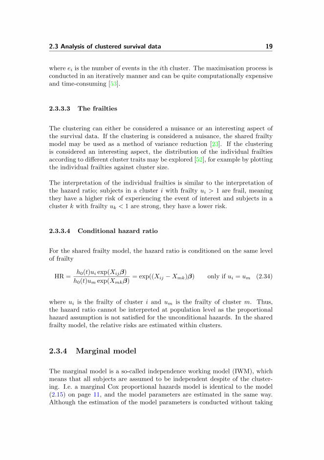
For the shared frailty model, the hazard ratio is conditioned on the same levelof frailty
HR =h0(t)ui exp(Xijβ)
h0(t)um exp(Xmkβ)= exp((Xij −Xmk)β) only if ui = um (2.34)
where ui is the frailty of cluster i and um is the frailty of cluster m. Thus,the hazard ratio cannot be interpreted at population level as the proportionalhazard assumption is not satisfied for the unconditional hazards. In the sharedfrailty model, the relative risks are estimated within clusters.
2.3.4 Marginal model
The marginal model is a so-called independence working model (IWM), whichmeans that all subjects are assumed to be independent despite of the cluster-ing. I.e. a marginal Cox proportional hazards model is identical to the model(2.15) on page 11, and the model parameters are estimated in the same way.Although the estimation of the model parameters is conducted without taking

20 Theory
the clustering of subjects into account, the estimators are consistent under areasonable set of conditions [7, 51]. However, the information matrix obtainedby the IWM is not a consistent estimator of the asymptotic variance-covariancematrix. An approximation to the grouped jackknife estimator [31, 32] is appliedto obtain the robust variance estimator
I−1(β)S(β)ST (β)I−1(β) (2.35)
where I(β) and S(β) are the information matrix and the score vector, respec-tively, of the IWM for all observations. The expression of the robust varianceestimator is equivalent to the sandwich estimator [57].
2.3.5 Copula model
The copula model can be used to combine the marginal survival functions ofdifferent subjects in a cluster and thereby generate the joint survival function.The joint survival function is given as
S(t1, . . . , tni) = Cθ{S1(t1), . . . , Sni(tni)}, t1, . . . , tni ≥ 0 (2.36)
where Cθ(v1, . . . , vni) is a ni-dimensional copula function with parameter vectorθ, defined for (v1, . . . , vni) ∈ [0, 1]ni and taking values in [0, 1]. The copulamodel enables modeling of the dependence between the marginals expressed inthe parameter θ [2].
2.3.5.1 The Clayton-Oakes copula
The family of Archimedean copulas are very popular and most often applied tomultivariate survival data [7]. An Archimedean copula has the form
Cθ(v1, . . . , vni) = φθ(φ−1θ (v1) + . . .+ φ−1
θ (vni)) (2.37)
where φ is a decreasing function defined on [0,∞], taking values in [0, 1] andsatisfying φ(0) = 1. The Archimedean copula family is popular, because thecopulas are easily derived and are capable of capturing many kinds of depen-dence. For more details on Archimedean copulas see Genest and MacKay (1986),Nelsen (2006) and Trivedi and Zimmer (2007).
2.3 Analysis of clustered survival data 21
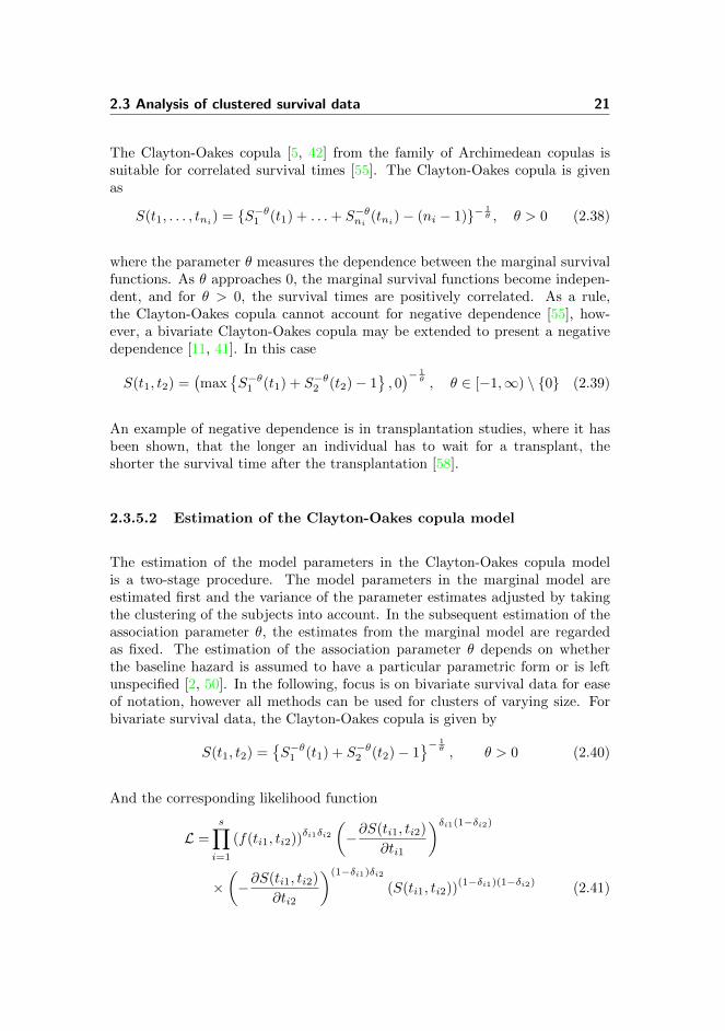
The Clayton-Oakes copula [5, 42] from the family of Archimedean copulas issuitable for correlated survival times [55]. The Clayton-Oakes copula is givenas
S(t1, . . . , tni) = {S−θ1 (t1) + . . .+ S−θni (tni)− (ni − 1)}− 1θ , θ > 0 (2.38)
where the parameter θ measures the dependence between the marginal survivalfunctions. As θ approaches 0, the marginal survival functions become indepen-dent, and for θ > 0, the survival times are positively correlated. As a rule,the Clayton-Oakes copula cannot account for negative dependence [55], how-ever, a bivariate Clayton-Oakes copula may be extended to present a negativedependence [11, 41]. In this case
S(t1, t2) =(max
{S−θ1 (t1) + S−θ2 (t2)− 1
}, 0)− 1
θ , θ ∈ [−1,∞) \ {0} (2.39)
An example of negative dependence is in transplantation studies, where it hasbeen shown, that the longer an individual has to wait for a transplant, theshorter the survival time after the transplantation [58].
2.3.5.2 Estimation of the Clayton-Oakes copula model
The estimation of the model parameters in the Clayton-Oakes copula modelis a two-stage procedure. The model parameters in the marginal model areestimated first and the variance of the parameter estimates adjusted by takingthe clustering of the subjects into account. In the subsequent estimation of theassociation parameter θ, the estimates from the marginal model are regardedas fixed. The estimation of the association parameter θ depends on whetherthe baseline hazard is assumed to have a particular parametric form or is leftunspecified [2, 50]. In the following, focus is on bivariate survival data for easeof notation, however all methods can be used for clusters of varying size. Forbivariate survival data, the Clayton-Oakes copula is given by
S(t1, t2) ={S−θ1 (t1) + S−θ2 (t2)− 1
}− 1θ , θ > 0 (2.40)
And the corresponding likelihood function
L =
s∏i=1
(f(ti1, ti2))δi1δi2
(−∂S(ti1, ti2)
∂ti1
)δi1(1−δi2)
×(−∂S(ti1, ti2)
∂ti2
)(1−δi1)δi2
(S(ti1, ti2))(1−δi1)(1−δi2)
(2.41)
22 Theory
Parametric baseline If the survival times are assumed to follow a givendistribution, the association parameter θ is estimated by maximisation of thelikelihood function given in (2.41), where the estimated parameters from themarginal model have been plugged in. If the baseline is parametric, the param-eters β and θ may also be estimated simultaneously [17], but the computationsquickly become very complicated [2].
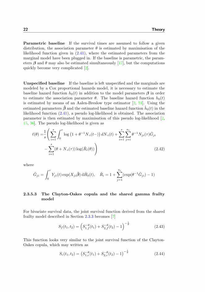
Unspecified baseline If the baseline is left unspecified and the marginals aremodeled by a Cox proportional hazards model, it is necessary to estimate thebaseline hazard function h0(t) in addition to the model parameters β in orderto estimate the association parameter θ. The baseline hazard function h0(t)is estimated by means of an Aalen-Breslow type estimator [2, 51]. Using the
estimated parameters β and the estimated baseline hazard function h0(t) in thelikelihood function (2.41), a pseudo log-likelihood is obtained. The associationparameter is then estimated by maximisation of this pseudo log-likelihood [2,15, 36]. The pseudo log-likelihood is given as
`(θ) =1
s
(s∑i=1
∫ τ
0
log(1 + θ−1N·i(t−)
)dN·i(t) +
s∑i=1
ni∑j=i
θ−1Nji(τ)Gji
−s∑i=1
(θ +N·i(τ)) log(Ri(θ))
)(2.42)
where
Gji =
∫ τ
0
Yji(t) exp(Xjiβ) dH0(t), Ri = 1 +
ni∑j=1
(exp(θ−1Gji)− 1)
2.3.5.3 The Clayton-Oakes copula and the shared gamma frailtymodel
For bivariate survival data, the joint survival function derived from the sharedfrailty model described in Section 2.3.3 becomes [7]
Sf (t1, t2) =(S−θ1,f (t1) + S−θ2,f (t2)− 1
)− 1θ
(2.43)
This function looks very similar to the joint survival function of the Clayton-Oakes copula, which may written as
Sc(t1, t2) =(S−θ1,c (t1) + S−θ2,c (t2)− 1
)− 1θ (2.44)
2.4 Measure of dependence 23
Indeed, the joint survival function derived from the shared frailty model is alsoa Clayton-Oakes copula. However, even though the functional forms of the jointsurvival functions are identical, the two models are not equivalent and do notlead to the same parameter estimates because the marginal survival functions aremodelled differently [7, 17]. The difference is that the survival function Si,f (ti)from the conditional shared frailty model is also a function of the parameter θ,whereas the survival function Si,c(ti) from the Clayton-Oakes copula is not, cf.Section 2.3.3.2 and Section 2.3.5.2.
2.4 Measure of dependence
The shared frailty model and the Clayton-Oakes copula model described in Sec-tion 2.3.3 and in Section 2.3.5, respectively, can both be applied for estimationof the degree of dependence between clustered survival data. The shared frailtymodel estimates the variance θf of the frailties, and the copula model estimatesthe association parameter θc. The two parameters are somewhat similar due tothe concordance of the two models (cf. previous section).
The parameters θf and θc can be considered as measures of correlation of thesurvival times within clusters. For both models applies that if θ approaches 0,there is no dependence between the survival times of the subjects in a clusterand if θ is greater than 0, the survival times are positively correlated. Asmentioned, the bivariate Clayton-Oakes copula may be extended to present anegative dependence, in this case the survival times are negatively correlated ifθ < 0. For negatively correlated survival times, there is no frailty interpretation[23].
Just like any of the other model parameters, the significance of the parameter θcan be evaluated using a Wald or a likelihood ratio test. According to Therneauand Gramsch (2000) and Therneau et al. (2003), the likelihood ratio test ispreferable.
2.4.0.4 Kendall’s τ
The degree of dependence of bivariate survival data may be evaluated usingKendall’s τ [10, 52], which gives a generalised measure of the correlation betweenthe survival times. For the shared frailty model, Kendall’s τ is given as
τ =θf
(θf + 2), θf > 0 (2.45)
24 Theory
As seen, Kendall’s τ will be between 0 and 1. For the extended bivariateClayton-Oakes copula, Kendall’s τ is given by the same formula but definedon a wider interval
τ =θc
(θc + 2), θc ∈ [−1,∞) \ {0} (2.46)
Here, Kendall’s τ will be between −1 and 1.

Chapter 3
Materials & Methods
The purpose of this study is to investigate and compare different statisticalmethods for analysis of clustered survival data by means of data from a largeDanish register-based family study of the psychological late effects of exposureto childhood cancer. First, however, the statistical methods are explored usingthree smaller data sets, which are available through the statistical software R[48]. In this chapter, the three small data sets as well as the data from theregister-based family study are presented. In addition, it will be described howthe statistical analyses have been conducted.
3.1 Data
The three small data sets, which are available through different R packages aredescribed in the following section, after which the data from the register-basedfamily study of the late effects of childhood cancer is presented.
26 Materials & Methods
3.1.1 Data sets available through R
The three data sets are
• The diabetic retinopathy data (timereg package)
• The kidney catheter data (survival package)
• The NCCTG lung cancer data (survival package)
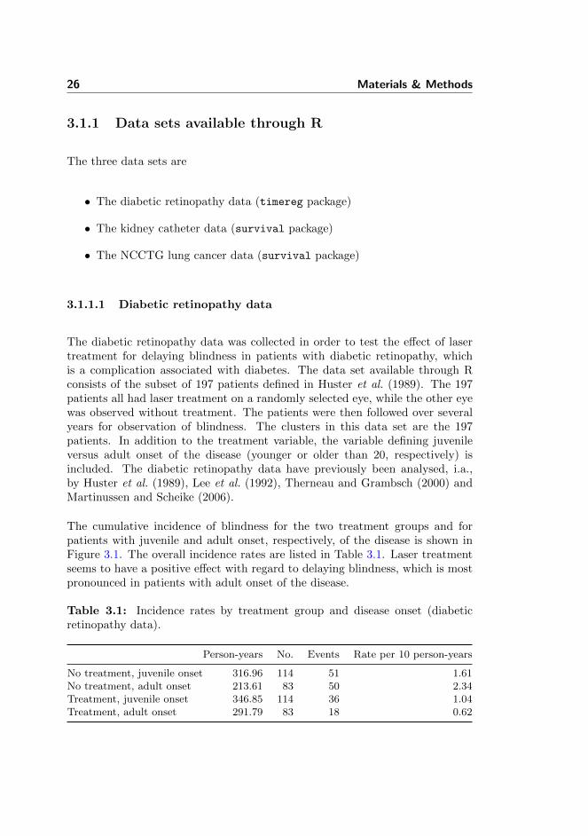
3.1.1.1 Diabetic retinopathy data
The diabetic retinopathy data was collected in order to test the effect of lasertreatment for delaying blindness in patients with diabetic retinopathy, whichis a complication associated with diabetes. The data set available through Rconsists of the subset of 197 patients defined in Huster et al. (1989). The 197patients all had laser treatment on a randomly selected eye, while the other eyewas observed without treatment. The patients were then followed over severalyears for observation of blindness. The clusters in this data set are the 197patients. In addition to the treatment variable, the variable defining juvenileversus adult onset of the disease (younger or older than 20, respectively) isincluded. The diabetic retinopathy data have previously been analysed, i.a.,by Huster et al. (1989), Lee et al. (1992), Therneau and Grambsch (2000) andMartinussen and Scheike (2006).
The cumulative incidence of blindness for the two treatment groups and forpatients with juvenile and adult onset, respectively, of the disease is shown inFigure 3.1. The overall incidence rates are listed in Table 3.1. Laser treatmentseems to have a positive effect with regard to delaying blindness, which is mostpronounced in patients with adult onset of the disease.
Table 3.1: Incidence rates by treatment group and disease onset (diabeticretinopathy data).
Person-years No. Events Rate per 10 person-years
No treatment, juvenile onset 316.96 114 51 1.61No treatment, adult onset 213.61 83 50 2.34Treatment, juvenile onset 346.85 114 36 1.04Treatment, adult onset 291.79 83 18 0.62
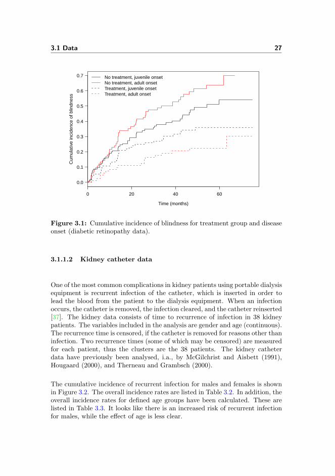
3.1 Data 27
0 20 40 60
0.0
0.1
0.2
0.3
0.4
0.5
0.6
0.7
Time (months)
Cum
ulat
ive
inci
denc
e of
blin
dnes
s
No treatment, juvenile onsetNo treatment, adult onsetTreatment, juvenile onsetTreatment, adult onset
Figure 3.1: Cumulative incidence of blindness for treatment group and diseaseonset (diabetic retinopathy data).
3.1.1.2 Kidney catheter data
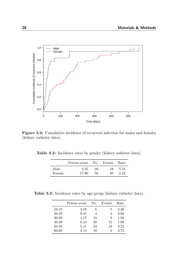
One of the most common complications in kidney patients using portable dialysisequipment is recurrent infection of the catheter, which is inserted in order tolead the blood from the patient to the dialysis equipment. When an infectionoccurs, the catheter is removed, the infection cleared, and the catheter reinserted[37]. The kidney data consists of time to recurrence of infection in 38 kidneypatients. The variables included in the analysis are gender and age (continuous).The recurrence time is censored, if the catheter is removed for reasons other thaninfection. Two recurrence times (some of which may be censored) are measuredfor each patient, thus the clusters are the 38 patients. The kidney catheterdata have previously been analysed, i.a., by McGilchrist and Aisbett (1991),Hougaard (2000), and Therneau and Grambsch (2000).
The cumulative incidence of recurrent infection for males and females is shownin Figure 3.2. The overall incidence rates are listed in Table 3.2. In addition, theoverall incidence rates for defined age groups have been calculated. These arelisted in Table 3.3. It looks like there is an increased risk of recurrent infectionfor males, while the effect of age is less clear.
28 Materials & Methods
0 100 200 300 400 500
0.0
0.2
0.4
0.6
0.8
1.0
Time (days)
Cum
ulat
ive
inci
denc
e of
rec
urre
nt in
fect
ion
MaleFemale
Figure 3.2: Cumulative incidence of recurrent infection for males and females(kidney catheter data).
Table 3.2: Incidence rates by gender (kidney catheter data).
Person-years No. Events Rate
Male 3.25 20 18 5.54Female 17.90 56 40 2.23
Table 3.3: Incidence rates by age group (kidney catheter data).
Person-years No. Events Rate
10-19 3.18 8 7 2.2020-29 0.41 4 4 9.6830-39 4.17 10 8 1.9240-49 6.13 20 12 1.9650-59 5.11 24 19 3.7260-69 2.14 10 8 3.74
3.1 Data 29
3.1.1.3 NCCTG lung cancer data
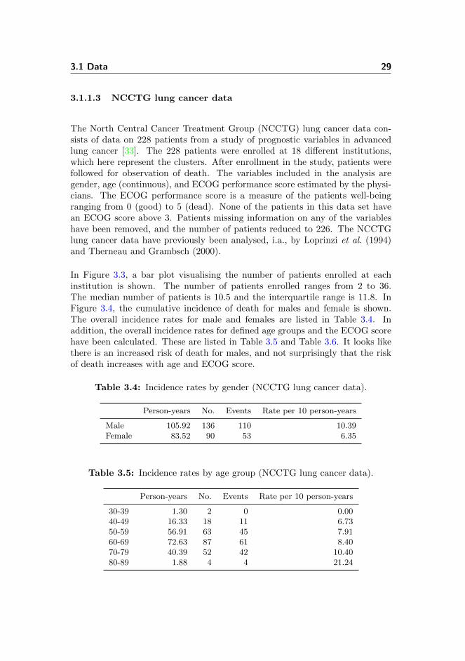
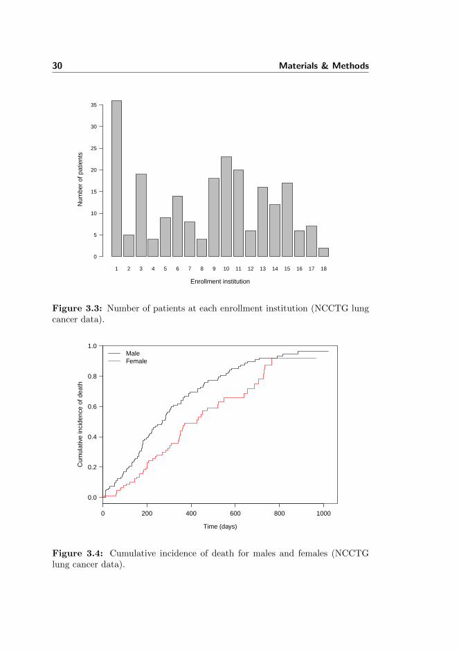
The North Central Cancer Treatment Group (NCCTG) lung cancer data con-sists of data on 228 patients from a study of prognostic variables in advancedlung cancer [33]. The 228 patients were enrolled at 18 different institutions,which here represent the clusters. After enrollment in the study, patients werefollowed for observation of death. The variables included in the analysis aregender, age (continuous), and ECOG performance score estimated by the physi-cians. The ECOG performance score is a measure of the patients well-beingranging from 0 (good) to 5 (dead). None of the patients in this data set havean ECOG score above 3. Patients missing information on any of the variableshave been removed, and the number of patients reduced to 226. The NCCTGlung cancer data have previously been analysed, i.a., by Loprinzi et al. (1994)and Therneau and Grambsch (2000).
In Figure 3.3, a bar plot visualising the number of patients enrolled at eachinstitution is shown. The number of patients enrolled ranges from 2 to 36.The median number of patients is 10.5 and the interquartile range is 11.8. InFigure 3.4, the cumulative incidence of death for males and female is shown.The overall incidence rates for male and females are listed in Table 3.4. Inaddition, the overall incidence rates for defined age groups and the ECOG scorehave been calculated. These are listed in Table 3.5 and Table 3.6. It looks likethere is an increased risk of death for males, and not surprisingly that the riskof death increases with age and ECOG score.
Table 3.4: Incidence rates by gender (NCCTG lung cancer data).
Person-years No. Events Rate per 10 person-years
Male 105.92 136 110 10.39Female 83.52 90 53 6.35
Table 3.5: Incidence rates by age group (NCCTG lung cancer data).
Person-years No. Events Rate per 10 person-years
30-39 1.30 2 0 0.0040-49 16.33 18 11 6.7350-59 56.91 63 45 7.9160-69 72.63 87 61 8.4070-79 40.39 52 42 10.4080-89 1.88 4 4 21.24
30 Materials & Methods
1 2 3 4 5 6 7 8 9 10 11 12 13 14 15 16 17 18
Enrollment institution
Num
ber
of p
atie
nts
0
5
10
15
20
25
30
35
Figure 3.3: Number of patients at each enrollment institution (NCCTG lungcancer data).
0 200 400 600 800 1000
0.0
0.2
0.4
0.6
0.8
1.0
Time (days)
Cum
ulat
ive
inci
denc
e of
dea
th
MaleFemale
Figure 3.4: Cumulative incidence of death for males and females (NCCTGlung cancer data).

3.1 Data 31
Table 3.6: Incidence rates by ECOG score (NCCTG lung cancer data).
ECOG score Person-years No. Events Rate per 10 person-years
0 60.69 63 37 6.101 97.28 113 82 8.432 31.14 49 43 13.813 0.32 1 1 30.95
3.1.2 Childhood cancer data
The childhood cancer data analysed in this study consists of data from a Danishregister-based family study of psychological late effects in families exposed tochildhood cancer. Research suggests that childhood cancer survivors, particularthose with central nervous system tumors, have poor psychological health [21,34, 60], and also siblings may suffer from from psychological distress [4]. Theoriginal cohort from the family study will be briefly described in the followingsection after which the analysed subset is presented.
3.1.2.1 Description of original cohort
The original cohort is based on 8561 children diagnosed with cancer in the pe-riod January 1 1975 to December 31 2009. The children were aged between0 and 19 at diagnosis and identified through the Danish Cancer Register [13].By means of the Danish Civil Registration System [44, 45], each of the childrenwere matched on gender and age to twenty children without cancer (at date ofdiagnosis). In the following, the children with cancer and their match are namedexposed and unexposed probands, respectively. The probands’ (both exposedand unexposed) full siblings and half siblings born no later than December 312009 (end of study period) were identified based on the personal identificationnumber of their parents through the Danish Civil Registration System and in-cluded in the cohort. The parents were also included in the cohort.
The Danish Civil Registration System was used to obtain date of death, dis-appearance and emigration (if any), and by linking the cohort to the DanishPsychiatric Central Research Register [40] admissions due to mental disorderwere identified. The incidence admission was defined as any admission due toa mental disorder between inclusion date and December 31 2009 (end of studyperiod). The inclusion date was date of diagnosis of the exposed proband. How-ever, for unborn siblings (at date of diagnosis) inclusion date was date of birth.
32 Materials & Methods
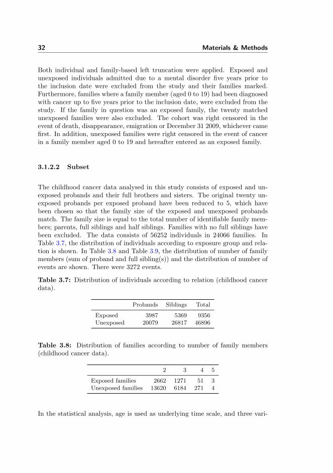
Both individual and family-based left truncation were applied. Exposed andunexposed individuals admitted due to a mental disorder five years prior tothe inclusion date were excluded from the study and their families marked.Furthermore, families where a family member (aged 0 to 19) had been diagnosedwith cancer up to five years prior to the inclusion date, were excluded from thestudy. If the family in question was an exposed family, the twenty matchedunexposed families were also excluded. The cohort was right censored in theevent of death, disappearance, emigration or December 31 2009, whichever camefirst. In addition, unexposed families were right censored in the event of cancerin a family member aged 0 to 19 and hereafter entered as an exposed family.
3.1.2.2 Subset
The childhood cancer data analysed in this study consists of exposed and un-exposed probands and their full brothers and sisters. The original twenty un-exposed probands per exposed proband have been reduced to 5, which havebeen chosen so that the family size of the exposed and unexposed probandsmatch. The family size is equal to the total number of identifiable family mem-bers; parents, full siblings and half siblings. Families with no full siblings havebeen excluded. The data consists of 56252 individuals in 24066 families. InTable 3.7, the distribution of individuals according to exposure group and rela-tion is shown. In Table 3.8 and Table 3.9, the distribution of number of familymembers (sum of proband and full sibling(s)) and the distribution of number ofevents are shown. There were 3272 events.
Table 3.7: Distribution of individuals according to relation (childhood cancerdata).
Probands Siblings Total
Exposed 3987 5369 9356Unexposed 20079 26817 46896
Table 3.8: Distribution of families according to number of family members(childhood cancer data).
2 3 4 5
Exposed families 2662 1271 51 3Unexposed families 13620 6184 271 4
In the statistical analysis, age is used as underlying time scale, and three vari-
3.1 Data 33
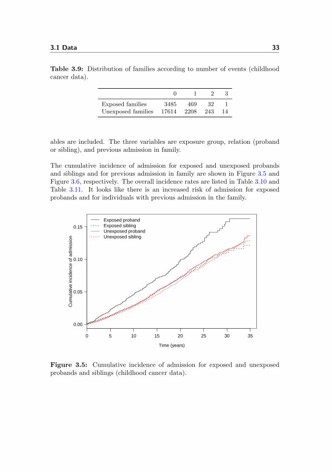
Table 3.9: Distribution of families according to number of events (childhoodcancer data).
0 1 2 3
Exposed families 3485 469 32 1Unexposed families 17614 2208 243 14
ables are included. The three variables are exposure group, relation (probandor sibling), and previous admission in family.
The cumulative incidence of admission for exposed and unexposed probandsand siblings and for previous admission in family are shown in Figure 3.5 andFigure 3.6, respectively. The overall incidence rates are listed in Table 3.10 andTable 3.11. It looks like there is an increased risk of admission for exposedprobands and for individuals with previous admission in the family.
0 5 10 15 20 25 30 35
0.00
0.05
0.10
0.15
Time (years)
Cum
ulat
ive
inci
denc
e of
adm
issi
on
Exposed probandExposed siblingUnexposed probandUnexposed sibling
Figure 3.5: Cumulative incidence of admission for exposed and unexposedprobands and siblings (childhood cancer data).

34 Materials & Methods
0 5 10 15 20 25 30 35
0.00
0.05
0.10
0.15
0.20
Time (years)
Cum
ulat
ive
inci
denc
e of
adm
issi
on
Previous admission in familyNo previous admission in family
Figure 3.6: Cumulative incidence of admission for variable previous admissionin family (childhood cancer data).
Table 3.10: Incidence rates by exposure group (childhood cancer data).
Person-years No. Events Rate per 103 person-years
Exposed proband 43236 3987 220 5.09Exposed sibling 86513 5369 316 3.65Unexposed proband 322557 20079 1205 3.74Unexposed sibling 432550 26817 1531 3.54
Table 3.11: Incidence rates by previous admission in family (childhood cancerdata).
Person-years No. Events Rate per 103 person-years
Previous admission 23494 1800 169 7.19No previous admission 861362 54452 3103 3.60
3.2 Statistical analysis 35
3.2 Statistical analysis
The statistical analyses in this study have all been conducted using the sta-tistical software R version 2.14.1 [48] by means of the two packages survival
and timereg. As mentioned, only semi-parametric models based on the Coxproportional hazards model have been fitted to the data.
The function coxph in the package survival has been applied to fit the unad-justed Cox proportional hazards model, the fixed effects model, the stratifiedmodel, and the shared frailty model. The shared frailty model are fitted usingthe penalised partial likelihood approach [53].
The proportional hazard assumption has been tested by means of the Schoenfeldresiduals using the function cox.zph also from the package survival. Thelinearity assumption has been tested by means of restricted cubic splines usingthe function cph in the rms package.
The function cox.aalen in the package timereg has been applied to fit themarginal Cox proportional hazards model, which is the first step of the esti-mation of the copula model. The function two.stage also from the packagetimereg has been applied to the second and final step of the estimation of thecopula model.
With regard to the significance of the parameters θf and θc from the sharedfrailty model and the copula model, respectively, they are evaluated using aWald test. The reason for this is, that it has not been possible to get an estimateof the log likelihood from the copula model using the timereg package.
The R code can be found in Appendix A.
36 Materials & Methods
Chapter 4
Results
In this chapter, the results of the statistical analyses are presented. First, theresults from the analyses of the three data sets available through the statisticalsoftware R will be presented. Hereafter, the results from the analyses of the datafrom the Danish register-based family study of the psychological late effects ofexposure to childhood cancer are presented.
4.1 Data sets available through R
4.1.1 Diabetic retinopathy data
The survival models that have been fitted to the diabetic retinopathy data arethe Cox proportional hazards model unadjusted for any patient effect, the Coxproportional hazards model stratified by patient, the shared gamma frailty Coxproportional hazards model, and the Clayton-Oakes copula with the marginalCox proportional hazards model as margin.
It was not possible to fit a Cox proportional hazards model with patient as a fixedeffect, as several patients did not experience blindness on either of their eyes.Thus the fixed effects model did not converge. Furthermore, the variable disease
38 Results
onset in the diabetic retinopathy data was nested within patient, and thus it wasnot possible to estimate the effect of this variable using the Cox proportionalhazards model stratified by patient. Therefore, in the Cox proportional hazardsmodel stratified by patient, the only variable included is treatment.
4.1.1.1 Unadjusted Cox proportional hazards model
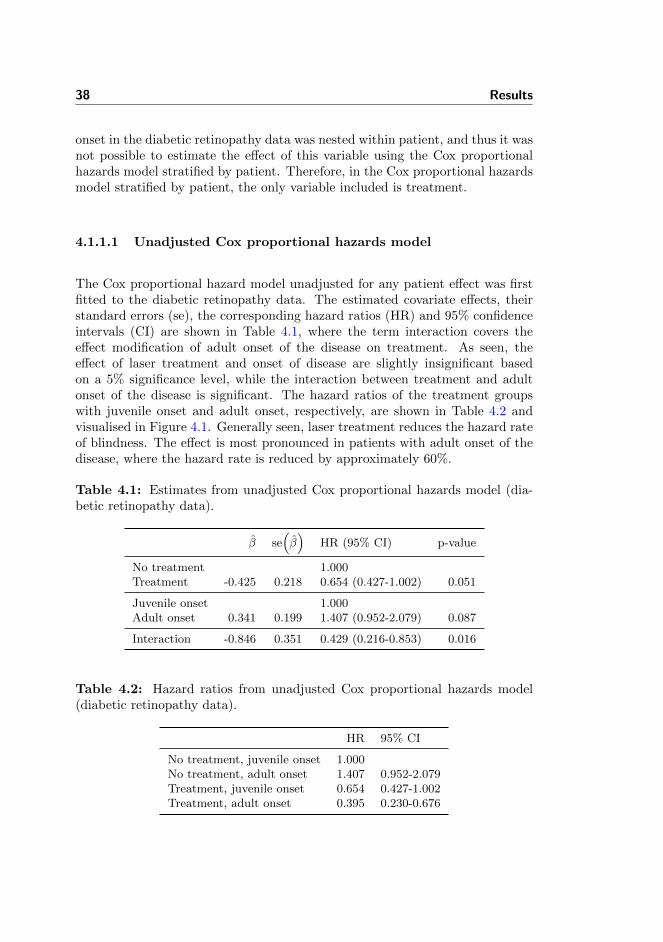
The Cox proportional hazard model unadjusted for any patient effect was firstfitted to the diabetic retinopathy data. The estimated covariate effects, theirstandard errors (se), the corresponding hazard ratios (HR) and 95% confidenceintervals (CI) are shown in Table 4.1, where the term interaction covers theeffect modification of adult onset of the disease on treatment. As seen, theeffect of laser treatment and onset of disease are slightly insignificant basedon a 5% significance level, while the interaction between treatment and adultonset of the disease is significant. The hazard ratios of the treatment groupswith juvenile onset and adult onset, respectively, are shown in Table 4.2 andvisualised in Figure 4.1. Generally seen, laser treatment reduces the hazard rateof blindness. The effect is most pronounced in patients with adult onset of thedisease, where the hazard rate is reduced by approximately 60%.
Table 4.1: Estimates from unadjusted Cox proportional hazards model (dia-betic retinopathy data).
β se(β)
HR (95% CI) p-value
No treatment 1.000Treatment -0.425 0.218 0.654 (0.427-1.002) 0.051
Juvenile onset 1.000Adult onset 0.341 0.199 1.407 (0.952-2.079) 0.087
Interaction -0.846 0.351 0.429 (0.216-0.853) 0.016
Table 4.2: Hazard ratios from unadjusted Cox proportional hazards model(diabetic retinopathy data).
HR 95% CI
No treatment, juvenile onset 1.000No treatment, adult onset 1.407 0.952-2.079Treatment, juvenile onset 0.654 0.427-1.002Treatment, adult onset 0.395 0.230-0.676
4.1 Data sets available through R 39
●
●
●
●
0.5
1.0
1.5
2.0H
R
No treatmentjuvenile onset
No treamentadult onset
Treatmentjuvenile onset
Treatmentadult onset
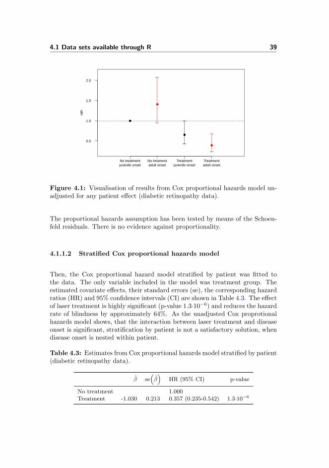
Figure 4.1: Visualisation of results from Cox proportional hazards model un-adjusted for any patient effect (diabetic retinopathy data).
The proportional hazards assumption has been tested by means of the Schoen-feld residuals. There is no evidence against proportionality.
4.1.1.2 Stratified Cox proportional hazards model
Then, the Cox proportional hazard model stratified by patient was fitted tothe data. The only variable included in the model was treatment group. Theestimated covariate effects, their standard errors (se), the corresponding hazardratios (HR) and 95% confidence intervals (CI) are shown in Table 4.3. The effectof laser treatment is highly significant (p-value 1.3·10−6) and reduces the hazardrate of blindness by approximately 64%. As the unadjusted Cox proprotionalhazards model shows, that the interaction between laser treatment and diseaseonset is significant, stratification by patient is not a satisfactory solution, whendisease onset is nested within patient.
Table 4.3: Estimates from Cox proportional hazards model stratified by patient(diabetic retinopathy data).
β se(β)
HR (95% CI) p-value
No treatment 1.000Treatment -1.030 0.213 0.357 (0.235-0.542) 1.3·10−6
40 Results
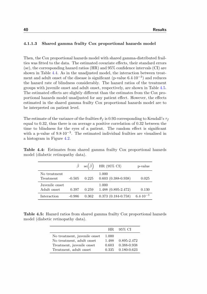
4.1.1.3 Shared gamma frailty Cox proportional hazards model
Then, the Cox proportional hazards model with shared gamma-distributed frail-ties was fitted to the data. The estimated covariate effects, their standard errors(se), the corresponding hazard ratios (HR) and 95% confidence intervals (CI) areshown in Table 4.4. As in the unadjusted model, the interaction between treat-ment and adult onset of the disease is significant (p-value 6.4·10−3) and reducesthe hazard rate of blindness considerably. The hazard ratios of the treatmentgroups with juvenile onset and adult onset, respectively, are shown in Table 4.5.The estimated effects are slightly different than the estimates from the Cox pro-portional hazards model unadjusted for any patient effect. However, the effectsestimated in the shared gamma frailty Cox proportional hazards model are tobe interpreted on patient level.
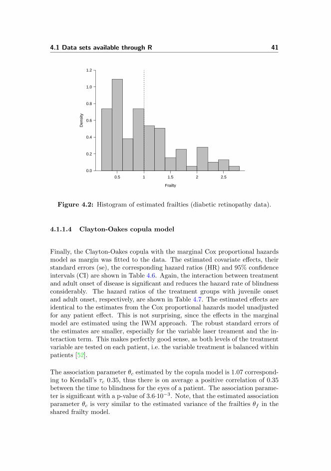
The estimate of the variance of the frailties θf is 0.93 corresponding to Kendall’s τfequal to 0.32, thus there is on average a positive correlation of 0.32 between thetime to blindness for the eyes of a patient. The random effect is significantwith a p-value of 9.8·10−3. The estimated individual frailties are visualised ina histogram in Figure 4.2.
Table 4.4: Estimates from shared gamma frailty Cox proportional hazardsmodel (diabetic retinopathy data).
β se(β)
HR (95% CI) p-value
No treatment 1.000Treatment -0.505 0.225 0.603 (0.388-0.938) 0.025
Juvenile onset 1.000Adult onset 0.397 0.259 1.488 (0.895-2.472) 0.130
Interaction -0.986 0.362 0.373 (0.184-0.758) 6.4·10−3
Table 4.5: Hazard ratios from shared gamma frailty Cox proportional hazardsmodel (diabetic retinopathy data).
HR 95% CI
No treatment, juvenile onset 1.000No treatment, adult onset 1.488 0.895-2.472Treatment, juvenile onset 0.603 0.388-0.938Treatment, adult onset 0.335 0.180-0.623
4.1 Data sets available through R 41
Frailty
Den
sity
0.0
0.2
0.4
0.6
0.8
1.0
1.2
0.5 1 1.5 2 2.5
Figure 4.2: Histogram of estimated frailties (diabetic retinopathy data).
4.1.1.4 Clayton-Oakes copula model
Finally, the Clayton-Oakes copula with the marginal Cox proportional hazardsmodel as margin was fitted to the data. The estimated covariate effects, theirstandard errors (se), the corresponding hazard ratios (HR) and 95% confidenceintervals (CI) are shown in Table 4.6. Again, the interaction between treatmentand adult onset of disease is significant and reduces the hazard rate of blindnessconsiderably. The hazard ratios of the treatment groups with juvenile onsetand adult onset, respectively, are shown in Table 4.7. The estimated effects areidentical to the estimates from the Cox proportional hazards model unadjustedfor any patient effect. This is not surprising, since the effects in the marginalmodel are estimated using the IWM approach. The robust standard errors ofthe estimates are smaller, especially for the variable laser treament and the in-teraction term. This makes perfectly good sense, as both levels of the treatmentvariable are tested on each patient, i.e. the variable treatment is balanced withinpatients [52].
The association parameter θc estimated by the copula model is 1.07 correspond-ing to Kendall’s τc 0.35, thus there is on average a positive correlation of 0.35between the time to blindness for the eyes of a patient. The association parame-ter is significant with a p-value of 3.6·10−3. Note, that the estimated associationparameter θc is very similar to the estimated variance of the frailties θf in theshared frailty model.

42 Results
Table 4.6: Estimates from margin of Clayton-Oakes copula model (diabeticretinopathy data).
β se(β)
HR (95% CI) p-value
No treatment 1.000Treatment -0.425 0.185 0.654 (0.455-0.940) 0.022
Juvenile onset 1.000Adult onset 0.341 0.196 1.407 (0.958-2.064) 0.081
Interaction -0.846 0.304 0.429 (0.237-0.778) 5.3·10−3
Table 4.7: Hazard ratios from margin of Clayton-Oakes copula model (diabeticretinopathy data).
HR 95% CI
No treatment, juvenile onset 1.000No treatment, adult onset 1.407 0.958-2.064Treatment, juvenile onset 0.654 0.455-0.940Treatment, adult onset 0.395 0.242-0.644
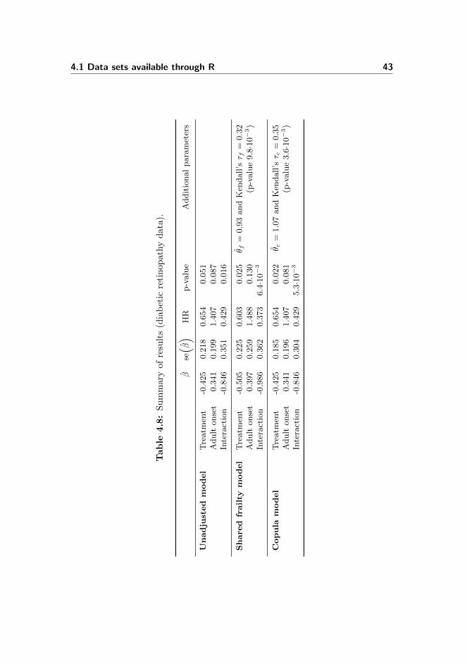
4.1.1.5 Summary of results
The estimated covariate effects, standard errors, hazard ratios and p-values fromthe survival models fitted to the diabetic retinopathy data are summarised inTable 4.8. The stratified model is omitted, since it is not comparable to theother fitted models.
4.1 Data sets available through R 43
Tab
le4.8
:S
um
mar
yof
resu
lts
(dia
bet
icre
tin
op
ath
yd
ata
).
βse( β
)HR
p-value
Additionalparameters
Unadju
sted
model
Treatm
ent
-0.425
0.218
0.654
0.051
Adult
onset
0.341
0.199
1.407
0.087
Interaction
-0.846
0.351
0.429
0.016
Share
dfr
ailty
model
Treatm
ent
-0.505
0.225
0.603
0.025
θ f=
0.93andKen
dall’sτ f
=0.32
Adult
onset
0.397
0.259
1.488
0.130
(p-value9.8·10−3)
Interaction
-0.986
0.362
0.373
6.4·10−3
Copula
model
Treatm
ent
-0.425
0.185
0.654
0.022
θ c=
1.07andKen
dall’sτ c
=0.35
Adult
onset
0.341
0.196
1.407
0.081
(p-value3.6·10−3)
Interaction
-0.846
0.304
0.429
5.3·10−3
44 Results
4.1.2 Kidney catheter data
The survival models that have been fitted to the kidney catheter data are theCox proportional hazards model unadjusted for any patient effect, the sharedgamma frailty Cox proportional hazards model, and the Clayton-Oakes copulawith the marginal Cox proportional hazards model as margin.
It was not possible to fit a Cox proportional hazards model with patient as afixed effect to the kidney data. Several patients did not experience recurrenceof infection, and thus the fixed effects model did not converge. Furthermore, itwas not possible to fit a Cox proportional hazards model stratified by patientto the kidney data. The variable gender was both nested within patients andthe variable age only varied for 11 out of the 38 patients and only by one year.
4.1.2.1 Unadjusted Cox proportional hazards model
The Cox proportional hazard model unadjusted for any patient effect was firstfitted to the kidney catheter data. There were no significant interaction be-tween the variable gender and the variable age (tested by means of likelihoodratio tests). The estimated covariate effects, their standard errors (se), the cor-responding hazard ratios (HR) and 95% confidence intervals (CI) are shown inTable 4.9. As seen, the effect of gender is significant based on a 5% significancelevel (p-value 5.5·10−3). The hazard rate of females is approximately 70% lowerthan the hazard rate of males. The effect of age is insignificant.
Table 4.9: Estimates from unadjusted Cox proportional hazards model (kidneycatheter data).
β se(β)
HR (95% CI) p-value
Male 1.000Female -0.829 0.299 0.436 (0.243-0.784) 5.5·10−3
Age (per 10 years) 0.020 0.092 1.021 (0.851-1.223) 0.826
The proportional hazards assumption have been tested by means of the Schoen-feld residuals. With regard to the variable gender there is evidence againstproportionality. However, this is because of an outlier, which will be elaboratedin a moment. The linearity assumption of the variable age has been evaluatedby means of a restricted cubic spline. In Figure 4.3, the relationship of age andthe log relative hazard is shown. It looks okay.

4.1 Data sets available through R 45
Adjusted to:sex=Female disease=Type 1 Age (years)
log
Rel
ativ
e H
azar
d
−1.5
−1.0
−0.5
0.0
0.5
20 30 40 50 60
Figure 4.3: Relationship between age and incidence recurrent infection (kidneycatheter data).
4.1.2.2 Shared gamma frailty Cox proportional hazards model
Then, the Cox proportional hazards model with shared gamma-distributed frail-ties was fitted to the data. The estimated covariate effects, their standard errors(se), the corresponding hazard ratios (HR) and 95% confidence intervals (CI)are shown in Table 4.10. In this model, the effect of gender is significant (p-value 5.7·10−4). The event rate of females is approximately 80% lower than thehazard rate of males. The estimated effects are different than the estimates fromthe Cox proportional hazards model unadjusted for any patient effect, especiallythe effect of gender. However, the effects estimated in the shared gamma frailtyCox proportional hazards model are to be interpreted on patient level.
The estimate of the variance of the frailties θf is 0.41 corresponding to Kendall’s τfequal to 0.17, thus there is on average a positive correlation of 0.17 between theinfection recurrence times. The random effect is significant with a p-value of0.04. The estimated individual frailties are visualised in a histogram in Fig-ure 4.4.
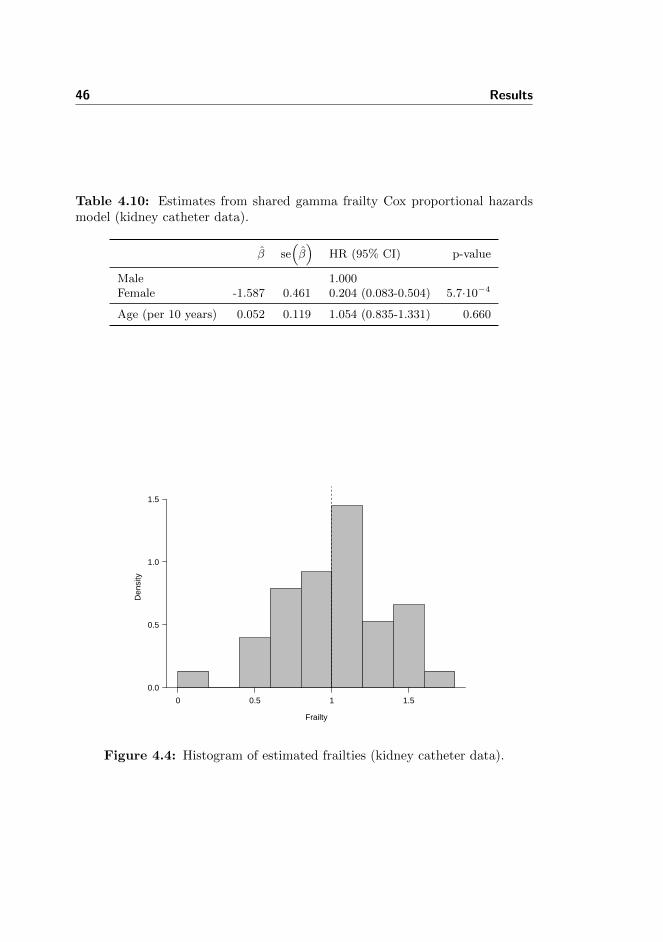
46 Results
Table 4.10: Estimates from shared gamma frailty Cox proportional hazardsmodel (kidney catheter data).
β se(β)
HR (95% CI) p-value
Male 1.000Female -1.587 0.461 0.204 (0.083-0.504) 5.7·10−4
Age (per 10 years) 0.052 0.119 1.054 (0.835-1.331) 0.660
Frailty
Den
sity
0.0
0.5
1.0
1.5
0 0.5 1 1.5
Figure 4.4: Histogram of estimated frailties (kidney catheter data).
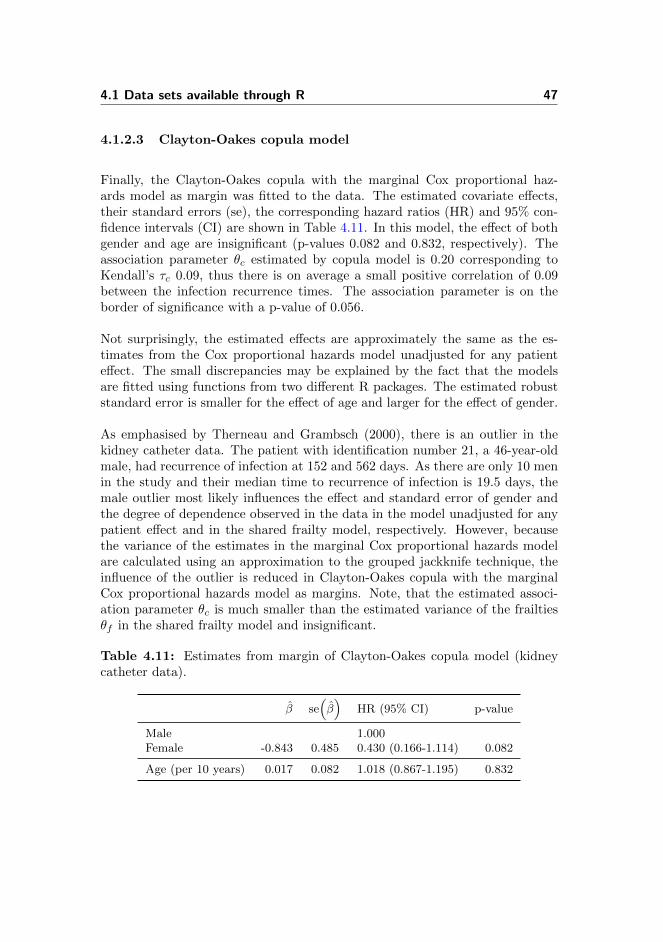
4.1 Data sets available through R 47
4.1.2.3 Clayton-Oakes copula model
Finally, the Clayton-Oakes copula with the marginal Cox proportional haz-ards model as margin was fitted to the data. The estimated covariate effects,their standard errors (se), the corresponding hazard ratios (HR) and 95% con-fidence intervals (CI) are shown in Table 4.11. In this model, the effect of bothgender and age are insignificant (p-values 0.082 and 0.832, respectively). Theassociation parameter θc estimated by copula model is 0.20 corresponding toKendall’s τc 0.09, thus there is on average a small positive correlation of 0.09between the infection recurrence times. The association parameter is on theborder of significance with a p-value of 0.056.
Not surprisingly, the estimated effects are approximately the same as the es-timates from the Cox proportional hazards model unadjusted for any patienteffect. The small discrepancies may be explained by the fact that the modelsare fitted using functions from two different R packages. The estimated robuststandard error is smaller for the effect of age and larger for the effect of gender.
As emphasised by Therneau and Grambsch (2000), there is an outlier in thekidney catheter data. The patient with identification number 21, a 46-year-oldmale, had recurrence of infection at 152 and 562 days. As there are only 10 menin the study and their median time to recurrence of infection is 19.5 days, themale outlier most likely influences the effect and standard error of gender andthe degree of dependence observed in the data in the model unadjusted for anypatient effect and in the shared frailty model, respectively. However, becausethe variance of the estimates in the marginal Cox proportional hazards modelare calculated using an approximation to the grouped jackknife technique, theinfluence of the outlier is reduced in Clayton-Oakes copula with the marginalCox proportional hazards model as margins. Note, that the estimated associ-ation parameter θc is much smaller than the estimated variance of the frailtiesθf in the shared frailty model and insignificant.
Table 4.11: Estimates from margin of Clayton-Oakes copula model (kidneycatheter data).
β se(β)
HR (95% CI) p-value
Male 1.000Female -0.843 0.485 0.430 (0.166-1.114) 0.082
Age (per 10 years) 0.017 0.082 1.018 (0.867-1.195) 0.832
48 Results
The analyses presented here have been repeated without the patient with iden-tification number 21. The parameter estimates from these analyses are sum-marised in Table B.1 on page 86 in Appendix B. Without this patient, neitherthe variance of frailties or the association parameter are significant. However,gender is significant in all models. Thus, if the patient with identification num-ber 21 is included in the analysis, the frailty in the shared frailty Cox propor-tional hazards model will account for the specific characteristics of this patients,while the Clayton-Oakes copula model with marginal Cox proportional hazardsmodel as margin will compensate with the association parameter and by in-creasing the robust standard errors.
4.1.2.4 Summary of results
The estimated covariate effects, standard errors, hazard ratios and p-valuesfrom the survival models fitted to the kidney catheter data are summarised inTable 4.12.
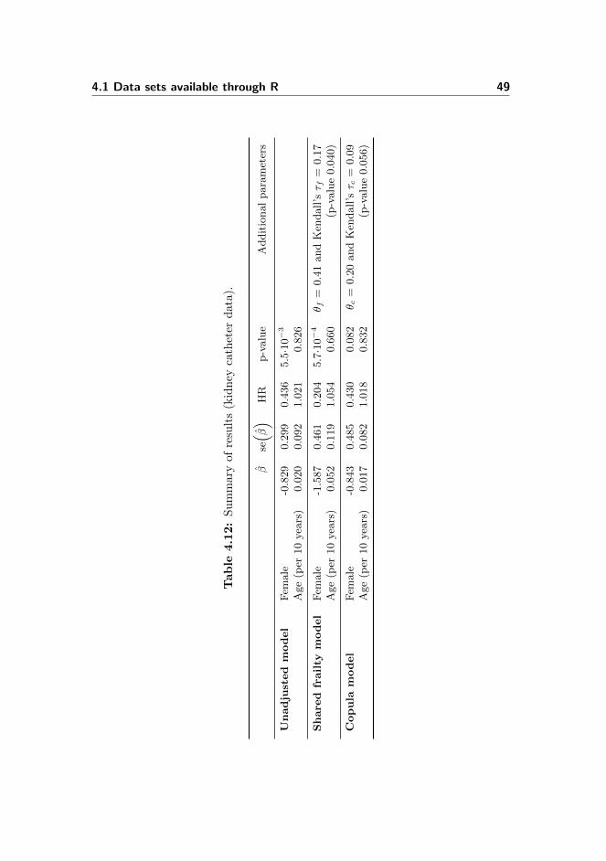
4.1 Data sets available through R 49
Tab
le4.1
2:
Su
mm
ary
ofre
sult
s(k
idn
eyca
thet
erd
ata
).
βse( β
)HR
p-value
Additionalparameters
Unadju
sted
model
Fem
ale
-0.829
0.299
0.436
5.5·10−3
Age(per
10years)
0.020
0.092
1.021
0.826
Share
dfr
ailty
model
Fem
ale
-1.587
0.461
0.204
5.7·10−4
θ f=
0.41andKen
dall’sτ f
=0.17
Age(per
10years)
0.052
0.119
1.054
0.660
(p-value0.040)
Copula
model
Fem
ale
-0.843
0.485
0.430
0.082
θ c=
0.20andKen
dall’sτ c
=0.09
Age(per
10years)
0.017
0.082
1.018
0.832
(p-value0.056)
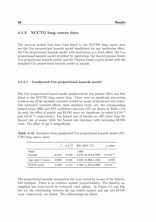
50 Results
4.1.3 NCCTG lung cancer data
The survival models that have been fitted to the NCCTG lung cancer dataare the Cox proportional hazards model unadjusted for any institution effect,the Cox proportional hazards model with institution as a fixed effect, the Coxproportional hazards model stratified by institution, the shared gamma frailtyCox proportional hazards model, and the Clayton-Oakes copula model with themarginal Cox proportional hazards model as margin.
4.1.3.1 Unadjusted Cox proportional hazards model
The Cox proportional hazard model unadjusted for any patient effect was firstfitted to the NCCTG lung cancer data. There were no significant interactionbetween any of the included variables (tested by means of likelihood ratio tests).The estimated covariate effects, their standard errors (se), the correspondinghazard ratios (HR) and 95% confidence intervals (CI) are shown in Table 4.13.As seen, the effect of gender and ECOG score are significant (p-values 9.3·10−4
and 4.0·10−5, respectively). The hazard rate of females are 43% lower than thehazard rate of males, while the hazard rate increases with increasing ECOGscore. The effect of age is insignificant.
Table 4.13: Estimates from unadjusted Cox proprotional hazards model (NC-CTG lung cancer data).
β se(β)
HR (95% CI) p-value
Male 1.000Female -0.557 0.168 0.573 (0.412-0.797) 9.3·10−4
Age (per 5 years) 0.056 0.046 1.058 (0.966-1.158) 0.225
ECOG score 0.469 0.114 1.599 (1.278-2.000) 4.0·10−5
The proportional hazards assumption has been tested by means of the Schoen-feld residuals. There is no evidence against proportionality. The linearity as-sumption has been tested by restricted cubic splines. In Figure 4.5 and Fig-ure 4.6, the relationship between the log relative hazard and age and ECOGscore, respectively, are shown. The relationships are linear.
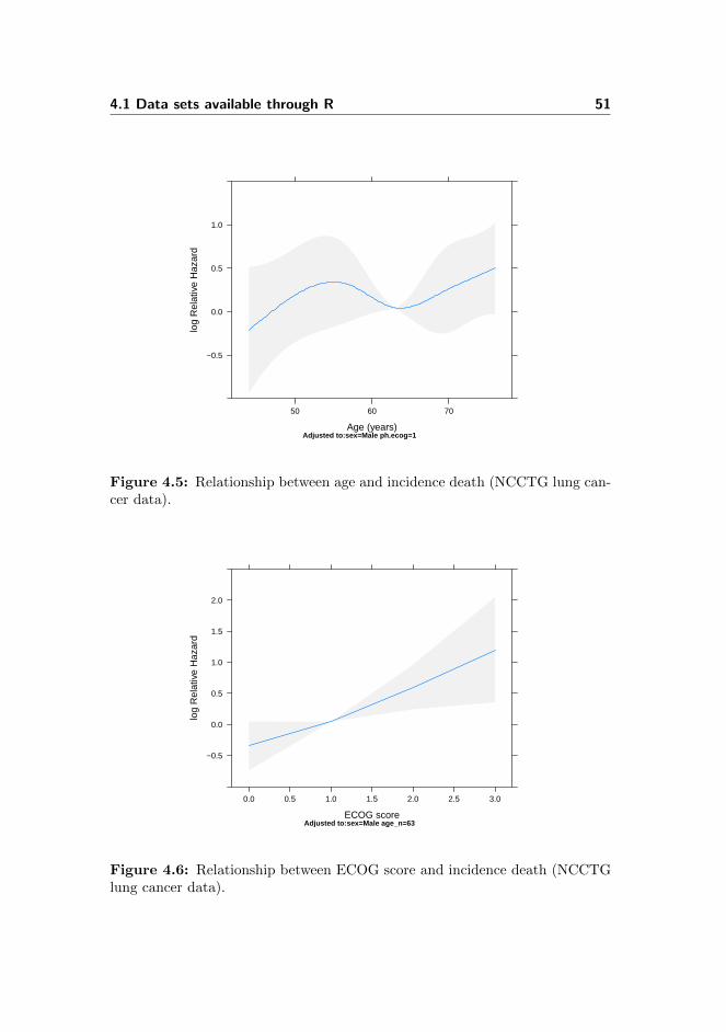
4.1 Data sets available through R 51
Adjusted to:sex=Male ph.ecog=1 Age (years)
log
Rel
ativ
e H
azar
d
−0.5
0.0
0.5
1.0
50 60 70
Figure 4.5: Relationship between age and incidence death (NCCTG lung can-cer data).
Adjusted to:sex=Male age_n=63 ECOG score
log
Rel
ativ
e H
azar
d
−0.5
0.0
0.5
1.0
1.5
2.0
0.0 0.5 1.0 1.5 2.0 2.5 3.0
Figure 4.6: Relationship between ECOG score and incidence death (NCCTGlung cancer data).

52 Results
4.1.3.2 Fixed effects Cox proportional hazards model
Then, the Cox proportional hazards model with enrollment institution as a fixedeffect was fitted to the data. The estimated covariate effects, their standarderrors (se), the corresponding hazard ratios (HR) and 95% confidence intervals(CI) are shown in Table 4.14. As seen, the effects of gender and ECOG scoreare significant (p-values 1.0·10−3 and 3.4·10−6, respectively), while the effectsof age and institution are not. Compared to the unadjusted Cox proportionalhazards model, the estimates change a bit, when institution is included as afixed effect. The overall significance of the institution variable has been testedin a likelihood ratio test and found to be insignificant (p-value 0.29). Some ofthe standard errors of the institution effects are quite large, since only a fewpatients are enrolled at these institutions.
Table 4.14: Estimates from Cox proportional model with institution as fixedeffect (NCCTG lung cancer data).
β se(β)
HR (95% CI) p-value
Male 1.000Female -0.571 0.174 0.565 (0.402-0.795) 1.0·10−3
Age (per 5 years) 0.049 0.049 1.051 (0.955-1.156) 0.312
ECOG score 0.604 0.130 1.829 (1.418-2.359) 3.4·10−6
Institution 1 1.000Institution 2 0.530 0.546 1.699 (0.583-4.951) 0.331Institution 3 -0.317 0.325 0.728 (0.386-1.376) 0.329Institution 4 -0.464 0.539 0.629 (0.218-1.809) 0.390Institution 5 0.034 0.456 1.034 (0.423-2.526) 0.941Institution 6 0.029 0.348 1.030 (0.520-2.037) 0.933Institution 7 -0.612 0.462 0.542 (0.219-1.342) 0.186Institution 8 0.495 0.543 1.640 (0.566-4.754) 0.362Institution 9 -0.547 0.360 0.578 (0.286-1.172) 0.128Institution 10 -0.119 0.308 0.887 (0.485-1.623) 0.698Institution 11 -0.522 0.351 0.593 (0.298-1.180) 0.137Institution 12 -0.508 0.544 0.602 (0.207-1.746) 0.350Institution 13 -0.718 0.362 0.488 (0.240-0.992) 0.047Institution 14 0.334 0.376 1.397 (0.669-2.917) 0.374Institution 15 -0.790 0.347 0.454 (0.230-0.896) 0.023Institution 16 -0.940 0.740 0.391 (0.092-1.665) 0.204Institution 17 -0.349 0.740 0.705 (0.165-3.006) 0.637Institution 18 0.472 1.030 1.603 (0.213-12.071) 0.647

4.1 Data sets available through R 53
4.1.3.3 Stratified Cox proportional hazards model
Then, the Cox proportional hazards model stratified by enrollment institutionwas fitted to the data. The estimated covariate effects, their standard errors(se), the corresponding hazard ratios (HR) and 95% confidence intervals (CI)are shown in Table 4.15. As before, the effect of gender and ECOG score aresignificant (p-values 2.6·10−3 and 1.5·10−5, respectively). The hazard rate offemales is approximately 42% lower than the hazard rate of males, while thehazard rate increases 82% with increasing ECOG score. The effect of age isinsignificant. The estimates are a bit different from the estimates from theunadjusted Cox proportional hazards model.
Table 4.15: Estimates from stratified Cox proportional hazards model (NC-CTG lung cancer data).
β se(β)
HR (95% CI) p-value
Male 1.000Female -0.547 0.182 0.578 (0.405-0.826) 2.6·10−3
Age (per 5 years) 0.048 0.051 1.049 (0.948-1.160) 0.353
ECOG score 0.597 0.138 1.817 (1.387-2.381) 1.5·10−5
4.1.3.4 Shared gamma frailty Cox proportional hazards model
Then, the Cox proportional hazards model with shared gamma-distributed frail-ties was fitted to the data. The estimated covariate effects, their standard errors(se), the corresponding hazard ratios (HR) and 95% confidence intervals (CI)are shown in Table 4.16. The estimated covariate effects and their standard er-ror are practically identical to the estimates from the Cox proportional hazardsmodel unadjusted for any patient effect. The explanation is straightforward; theestimate of the variance of the frailties θf is very small 8.4·10−3 and insignificant(p-value 0.27). Thus, there is no random effect of patient and the shared frailtymodel is reduced to the unadjusted Cox proportional hazards model. The esti-mated individual frailties are visualised in a histogram in Figure 4.7. As seen,they are distributed closely around 1.

54 Results
Table 4.16: Estimates from shared gamma frailty Cox proportional hazardsmodel (NCCTG lung cancer data).
β se(β)
HR (95% CI) p-value
Male 1.000Female -0.557 0.168 0.573 (0.412-0.797) 9.4·10−4
Age (per 5 years) 0.056 0.046 1.058 (0.965-1.159) 0.225
ECOG score 0.481 0.116 1.618 (1.290-2.029) 3.1·10−5
Frailty
Den
sity
0
5
10
15
0.92 0.96 1.00 1.04 1.08
Figure 4.7: Histogram of estimated frailties (NCCTG lung cancer data).
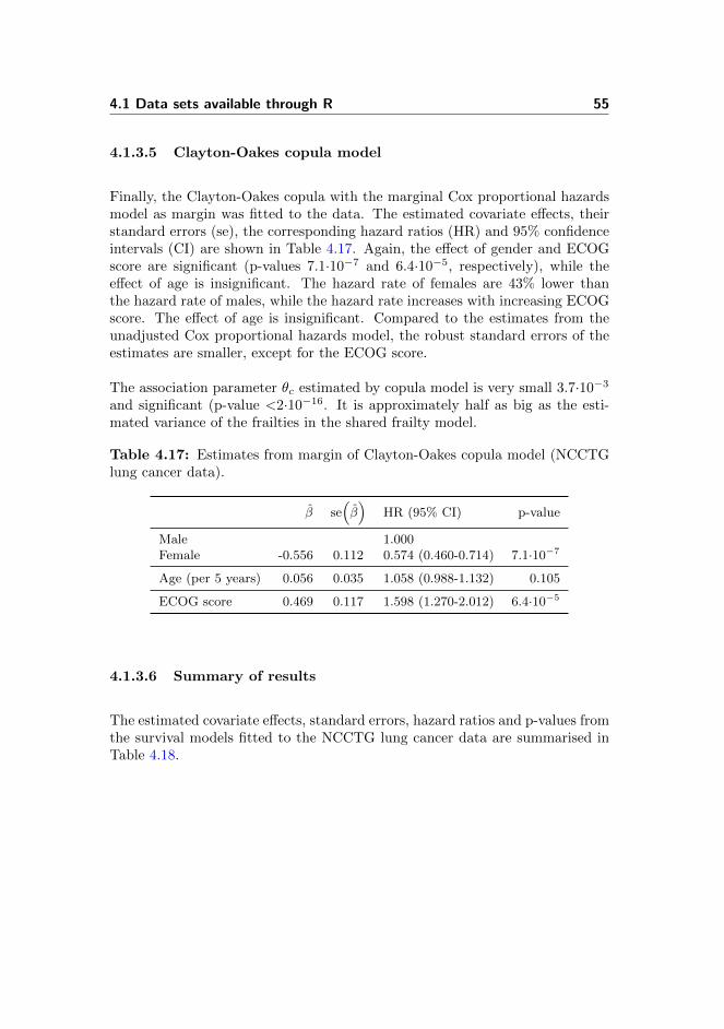
4.1 Data sets available through R 55
4.1.3.5 Clayton-Oakes copula model
Finally, the Clayton-Oakes copula with the marginal Cox proportional hazardsmodel as margin was fitted to the data. The estimated covariate effects, theirstandard errors (se), the corresponding hazard ratios (HR) and 95% confidenceintervals (CI) are shown in Table 4.17. Again, the effect of gender and ECOGscore are significant (p-values 7.1·10−7 and 6.4·10−5, respectively), while theeffect of age is insignificant. The hazard rate of females are 43% lower thanthe hazard rate of males, while the hazard rate increases with increasing ECOGscore. The effect of age is insignificant. Compared to the estimates from theunadjusted Cox proportional hazards model, the robust standard errors of theestimates are smaller, except for the ECOG score.
The association parameter θc estimated by copula model is very small 3.7·10−3
and significant (p-value <2·10−16. It is approximately half as big as the esti-mated variance of the frailties in the shared frailty model.
Table 4.17: Estimates from margin of Clayton-Oakes copula model (NCCTGlung cancer data).
β se(β)
HR (95% CI) p-value
Male 1.000Female -0.556 0.112 0.574 (0.460-0.714) 7.1·10−7
Age (per 5 years) 0.056 0.035 1.058 (0.988-1.132) 0.105
ECOG score 0.469 0.117 1.598 (1.270-2.012) 6.4·10−5
4.1.3.6 Summary of results
The estimated covariate effects, standard errors, hazard ratios and p-values fromthe survival models fitted to the NCCTG lung cancer data are summarised inTable 4.18.
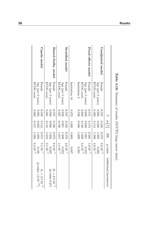
56 Results
Tab
le4.1
8:
Su
mm
aryof
results
(NC
CT
Glu
ng
can
cerd
ata
).
βse (
β )HR
p-va
lue
Additio
nalparameters
Unadju
sted
model
Fem
ale
-0.557
0.168
0.573
9.3·1
0−4
Age(per
5years)
0.056
0.046
1.058
0.225
ECOG
score
0.469
0.114
1.599
4.0·1
0−5
Fix
ed
eff
ects
model
Fem
ale
-0.571
0.174
0.565
1.0·1
0−3
Age(per
5years)
0.049
0.049
1.051
0.312
ECOG
score
0.604
0.130
1.829
3.4·1
0−6
Institu
tion2
0.530
0.546
1.699
0.331
...Institu
tion18
0.472
1.030
1.603
0.647
Stra
tified
model
Fem
ale
-0.547
0.182
0.578
2.6·1
0−3
Age(per
5years)
0.048
0.051
1.049
0.353
ECOG
score
0.597
0.138
1.817
1.5·1
0−5
Share
dfra
iltym
odel
Fem
ale
-0.557
0.168
0.573
9.4·1
0−4
θf=
8.5·1
0−3
Age(per
5years)
0.056
0.046
1.058
0.225
(p-va
lue0.27)
ECOG
score
0.481
0.116
1.618
3.1·1
0−5
Copula
model
Fem
ale
-0.556
0.112
0.574
7.1·1
0−7
θc=
3.7·1
0−3
Age(per
5years)
0.056
0.035
1.058
0.105
(p-va
lue<2·1
0−16)
ECOG
score
0.469
0.117
1.598
6.4·1
0−5
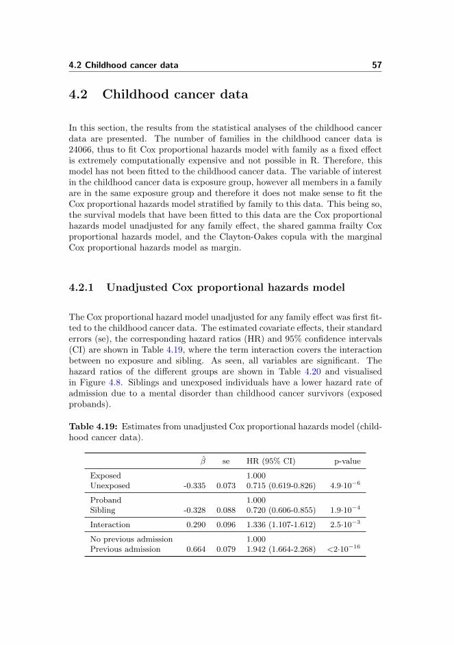
4.2 Childhood cancer data 57
4.2 Childhood cancer data
In this section, the results from the statistical analyses of the childhood cancerdata are presented. The number of families in the childhood cancer data is24066, thus to fit Cox proportional hazards model with family as a fixed effectis extremely computationally expensive and not possible in R. Therefore, thismodel has not been fitted to the childhood cancer data. The variable of interestin the childhood cancer data is exposure group, however all members in a familyare in the same exposure group and therefore it does not make sense to fit theCox proportional hazards model stratified by family to this data. This being so,the survival models that have been fitted to this data are the Cox proportionalhazards model unadjusted for any family effect, the shared gamma frailty Coxproportional hazards model, and the Clayton-Oakes copula with the marginalCox proportional hazards model as margin.
4.2.1 Unadjusted Cox proportional hazards model
The Cox proportional hazard model unadjusted for any family effect was first fit-ted to the childhood cancer data. The estimated covariate effects, their standarderrors (se), the corresponding hazard ratios (HR) and 95% confidence intervals(CI) are shown in Table 4.19, where the term interaction covers the interactionbetween no exposure and sibling. As seen, all variables are significant. Thehazard ratios of the different groups are shown in Table 4.20 and visualisedin Figure 4.8. Siblings and unexposed individuals have a lower hazard rate ofadmission due to a mental disorder than childhood cancer survivors (exposedprobands).
Table 4.19: Estimates from unadjusted Cox proportional hazards model (child-hood cancer data).
β se HR (95% CI) p-value
Exposed 1.000Unexposed -0.335 0.073 0.715 (0.619-0.826) 4.9·10−6
Proband 1.000Sibling -0.328 0.088 0.720 (0.606-0.855) 1.9·10−4
Interaction 0.290 0.096 1.336 (1.107-1.612) 2.5·10−3
No previous admission 1.000Previous admission 0.664 0.079 1.942 (1.664-2.268) <2·10−16
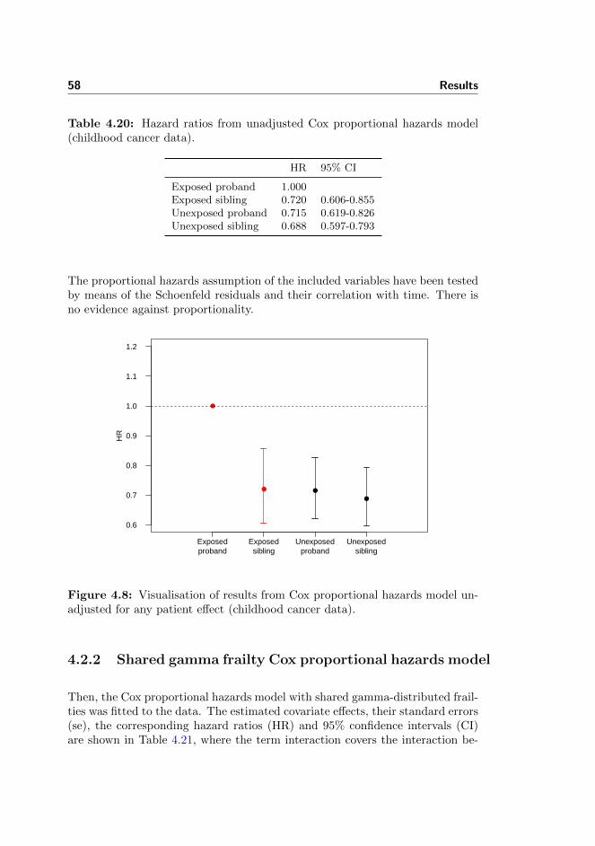
58 Results
Table 4.20: Hazard ratios from unadjusted Cox proportional hazards model(childhood cancer data).
HR 95% CI
Exposed proband 1.000Exposed sibling 0.720 0.606-0.855Unexposed proband 0.715 0.619-0.826Unexposed sibling 0.688 0.597-0.793
The proportional hazards assumption of the included variables have been testedby means of the Schoenfeld residuals and their correlation with time. There isno evidence against proportionality.
●
● ●
●
0.6
0.7
0.8
0.9
1.0
1.1
1.2
HR
Exposedproband
Exposedsibling
Unexposedproband
Unexposedsibling
Figure 4.8: Visualisation of results from Cox proportional hazards model un-adjusted for any patient effect (childhood cancer data).
4.2.2 Shared gamma frailty Cox proportional hazards model
Then, the Cox proportional hazards model with shared gamma-distributed frail-ties was fitted to the data. The estimated covariate effects, their standard errors(se), the corresponding hazard ratios (HR) and 95% confidence intervals (CI)are shown in Table 4.21, where the term interaction covers the interaction be-
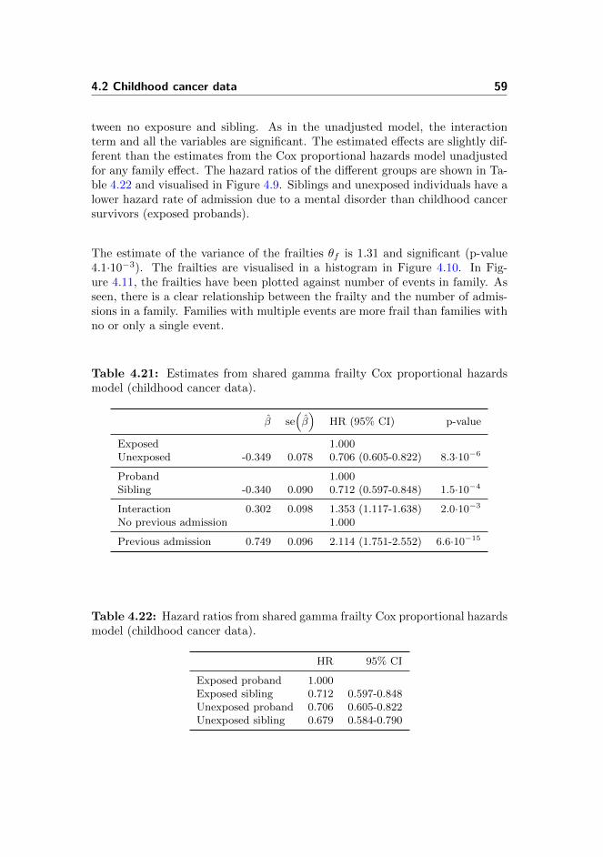
4.2 Childhood cancer data 59
tween no exposure and sibling. As in the unadjusted model, the interactionterm and all the variables are significant. The estimated effects are slightly dif-ferent than the estimates from the Cox proportional hazards model unadjustedfor any family effect. The hazard ratios of the different groups are shown in Ta-ble 4.22 and visualised in Figure 4.9. Siblings and unexposed individuals have alower hazard rate of admission due to a mental disorder than childhood cancersurvivors (exposed probands).
The estimate of the variance of the frailties θf is 1.31 and significant (p-value4.1·10−3). The frailties are visualised in a histogram in Figure 4.10. In Fig-ure 4.11, the frailties have been plotted against number of events in family. Asseen, there is a clear relationship between the frailty and the number of admis-sions in a family. Families with multiple events are more frail than families withno or only a single event.
Table 4.21: Estimates from shared gamma frailty Cox proportional hazardsmodel (childhood cancer data).
β se(β)
HR (95% CI) p-value
Exposed 1.000Unexposed -0.349 0.078 0.706 (0.605-0.822) 8.3·10−6
Proband 1.000Sibling -0.340 0.090 0.712 (0.597-0.848) 1.5·10−4
Interaction 0.302 0.098 1.353 (1.117-1.638) 2.0·10−3
No previous admission 1.000
Previous admission 0.749 0.096 2.114 (1.751-2.552) 6.6·10−15
Table 4.22: Hazard ratios from shared gamma frailty Cox proportional hazardsmodel (childhood cancer data).
HR 95% CI
Exposed proband 1.000Exposed sibling 0.712 0.597-0.848Unexposed proband 0.706 0.605-0.822Unexposed sibling 0.679 0.584-0.790
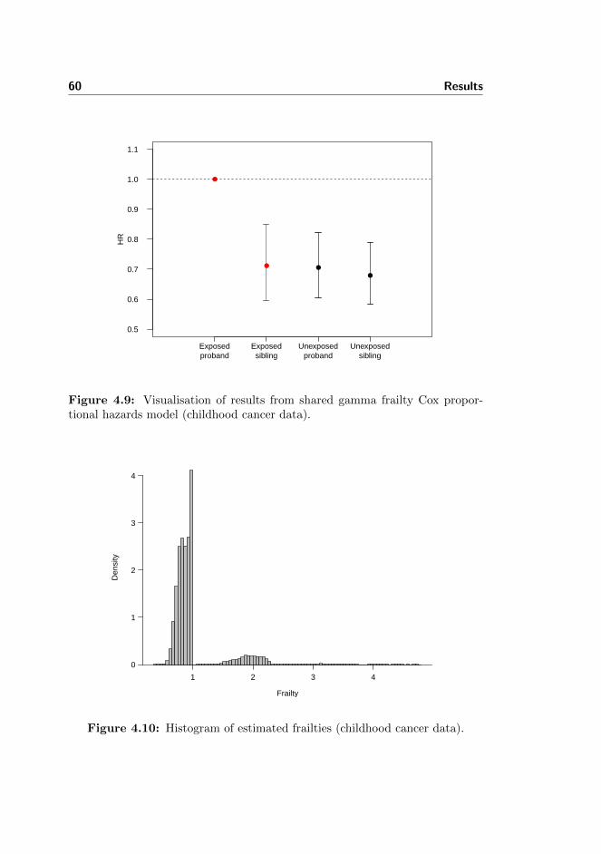
60 Results
●
● ●
●
0.5
0.6
0.7
0.8
0.9
1.0
1.1
HR
Exposedproband
Exposedsibling
Unexposedproband
Unexposedsibling
Figure 4.9: Visualisation of results from shared gamma frailty Cox propor-tional hazards model (childhood cancer data).
Frailty
Den
sity
0
1
2
3
4
1 2 3 4
Figure 4.10: Histogram of estimated frailties (childhood cancer data).
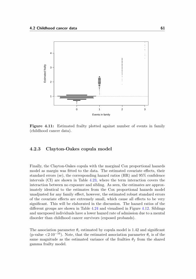
4.2 Childhood cancer data 61
1
2
3
4
Events in family
Est
imat
ed fr
ailty
0 1 2 3
Figure 4.11: Estimated frailty plotted against number of events in family(childhood cancer data).
4.2.3 Clayton-Oakes copula model
Finally, the Clayton-Oakes copula with the marginal Cox proportional hazardsmodel as margin was fitted to the data. The estimated covariate effects, theirstandard errors (se), the corresponding hazard ratios (HR) and 95% confidenceintervals (CI) are shown in Table 4.23, where the term interaction covers theinteraction between no exposure and sibling. As seen, the estimates are approx-imately identical to the estimates from the Cox proportional hazards modelunadjusted for any family effect, however, the estimated robust standard errorsof the covariate effects are extremely small, which cause all effects to be verysignificant. This will be elaborated in the discussion. The hazard ratios of thedifferent groups are shown in Table 4.24 and visualised in Figure 4.12. Siblingsand unexposed individuals have a lower hazard rate of admission due to a mentaldisorder than childhood cancer survivors (exposed probands).
The association parameter θc estimated by copula model is 1.42 and significant(p-value <2·10−16). Note, that the estimated association parameter θc is of thesame magnitude as the estimated variance of the frailties θf from the sharedgamma frailty model.
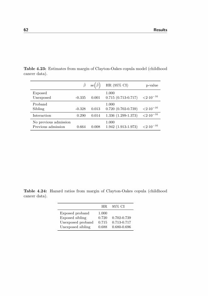
62 Results
Table 4.23: Estimates from margin of Clayton-Oakes copula model (childhoodcancer data).
β se(β)
HR (95% CI) p-value
Exposed 1.000Unexposed -0.335 0.001 0.715 (0.713-0.717) <2·10−16
Proband 1.000Sibling -0.328 0.013 0.720 (0.702-0.739) <2·10−16
Interaction 0.290 0.014 1.336 (1.299-1.373) <2·10−16
No previous admission 1.000Previous admission 0.664 0.008 1.942 (1.913-1.973) <2·10−16
Table 4.24: Hazard ratios from margin of Clayton-Oakes copula (childhoodcancer data).
HR 95% CI
Exposed proband 1.000Exposed sibling 0.720 0.702-0.739Unexposed proband 0.715 0.713-0.717Unexposed sibling 0.688 0.680-0.696
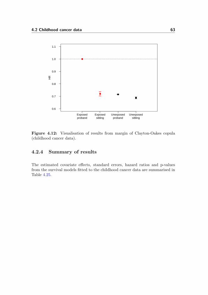
4.2 Childhood cancer data 63
●
● ●
●
0.6
0.7
0.8
0.9
1.0
1.1H
R
Exposedproband
Exposedsibling
Unexposedproband
Unexposedsibling
Figure 4.12: Visualisation of results from margin of Clayton-Oakes copula(childhood cancer data).
4.2.4 Summary of results
The estimated covariate effects, standard errors, hazard ratios and p-valuesfrom the survival models fitted to the childhood cancer data are summarised inTable 4.25.
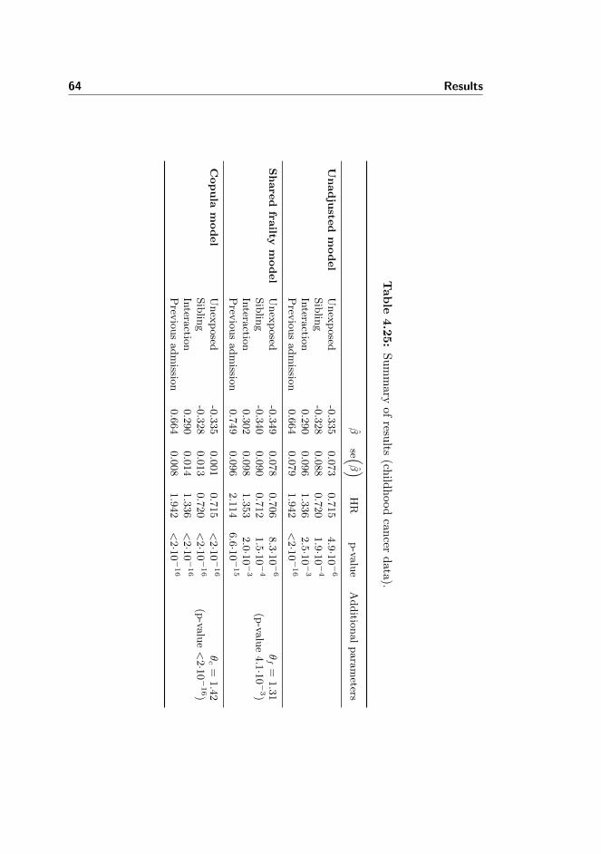
64 Results
Tab
le4.2
5:
Su
mm
aryof
results
(child
hood
can
cerd
ata
).
βse (
β )HR
p-va
lue
Additio
nalparameters
Unadju
sted
model
Unexposed
-0.335
0.073
0.715
4.9·1
0−6
Siblin
g-0.328
0.088
0.720
1.9·1
0−4
Intera
ction
0.290
0.096
1.336
2.5·1
0−3
Prev
iousadmissio
n0.664
0.079
1.942
<2·1
0−16
Share
dfra
iltym
odel
Unexposed
-0.349
0.078
0.706
8.3·1
0−6
θf=
1.31
Siblin
g-0.340
0.090
0.712
1.5·1
0−4
(p-va
lue4.1·1
0−3)
Intera
ction
0.302
0.098
1.353
2.0·1
0−3
Prev
iousadmissio
n0.749
0.096
2.114
6.6·1
0−15
Copula
model
Unexposed
-0.335
0.001
0.715
<2·1
0−16
θc=
1.42
Siblin
g-0.328
0.013
0.720
<2·1
0−16
(p-va
lue<2·1
0−16)
Intera
ction
0.290
0.014
1.336
<2·1
0−16
Prev
iousadmissio
n0.664
0.008
1.942
<2·1
0−16

Chapter 5
Discussion
In this chapter, the statistical methods will be discussed based on the resultspresented in the previous chapter. In addition, extensions of the applied meth-ods will be presented and suggestions for further work will be given.
5.1 Data sets available through R
As illustrated by the three data examples, natural clustering of study subjectsarises in different situations and for different kinds of data.
When cluster sizes are small relative to the number of clusters, introductionof a fixed effect for each cluster is generally not a good solution, and in somesituations it is not even possible. With regard to the data sets available throughR, it was only possible to fit the Cox proportional hazards model with cluster as afixed effect to one out of the three; the NCCTG lung cancer data. In the diabeticretinopathy data and the kidney catheter data, there were clusters without anyevents, where it was not possible to estimate a cluster effect, and thus the modeldid not converge. With regard to the model fitted to the NCCTG lung cancerdata, the standard errors for some of the cluster effects were very large because ofa limited number of subjects in these clusters. Although, data was adjusted for
66 Discussion
clustering, the introduction of a fixed cluster effect did not contribute valuableinformation to the analysis but reduced the degrees of freedom.
Stratification by cluster allows each cluster to have its own unspecified baseline.This approach is normally used to accommodate covariates that do not satisfythe proportional hazard assumption [27]. Although this model is more flexiblethan the fixed effects model [7], it is inefficient, when the covariates of interestare nested within the clusters as was the case with both the diabetic retinopathydata and the kidney catheter data. When the clustering is on a higher level asin the NCTTG lung cancer data, i.e. institution versus patient, stratification bycluster is a reasonable solution. With regard to the NCCTG lung cancer data,the effect estimates were similar to that of the Cox proportional hazards modelunadjusted for any cluster effect, although the standard errors were somewhathigher. This may be explained by the fact that a cluster only contributes to thepartial likelihood if an event is observed, while at least one other subject is stillat risk [7, 23].
It was possible to fit the shared frailty model to all three data sets, however thevariance of the frailty parameter was only significant in the diabetic retinopa-thy data and in the kidney catheter data. The estimated effects were slightlydifferent from the estimates from the model unadjusted for any patient effect,however, this is not surprising, as the covariate effects are conditioned on thefrailty and have to be interpreted on cluster level. For the NCCTG lung cancerdata, the variance of the frailty was approximately zero, and the shared frailtymodel was practically reduced to the model unadjusted for any cluster effect.
The Clayton-Oakes copula modula with the marginal Cox proportional hazardsmodel as margin was like the shared frailty model fitted to all three data sets.As the marginal Cox proportional hazards model is an IWM, the effect esti-mates were identical to the estimates from the Cox proportional hazards modelunadjusted for any cluster effect, while the standard errors varied. With regardto the diabetic retinopathy data, the estimated association parameter was sig-nificant and very similar to the variance of the frailty parameter in the sharedfrailty model. There was an outlier in the kidney catheter data, which affectedboth the shared frailty model and the copula model. The characteristics of theoutlier was accounted for by the frailty in the shared frailty model, while theClayton-Oakes copula model with marginal Cox proportional hazards modelas margin compensated by means of the association parameter and the robuststandard errors, see Table 4.12 and Table B.1 on page 49 and 86, respectively.
5.2 Childhood cancer data 67
5.2 Childhood cancer data
Three different statistical models were applied in the analysis of the data fromthe Danish register-based study of incident admission due to mental disorder infamilies exposed to childhood cancer. The three models were
• The Cox proportional hazards model unadjusted for any family effect
• The shared gamma frailty Cox proportional hazards model
• The Clayton-Oakes copula with the marginal Cox proportional hazardsmodel as margin
All three models showed that individuals diagnosed with cancer and individualswith a family history of admission due to mental disorders have an increasedhazard rate. Having a sister or brother diagnosed with cancer did not increasethe hazard rate.
5.2.1 Degree of dependence
The variance of the frailty parameter in the shared gamma frailty Cox propor-tional hazards model was significant, thus the event times within a family waspositively correlated. As seen in Figure 4.11 on page 61, there was a clear rela-tionship between the number of events and the frailty of a family; families withmultiple events were more frail than families with no or only a single event.This is not surprising, as the individual frailties may be considered as unob-served risk factors. The association parameter estimated in the Clayton-Oakescopula model was also significant, and somewhat similar to the variance of thefrailty parameter.
5.2.2 Robust standard errors
The robust standard errors of the estimated covariate effects in the Clayton-Oakes copula model with the marginal Cox proportional hazards model as mar-gin, were extremely small, which caused all variables to be significant, see Ta-ble 5.1. The marginal model was fitted using the function cox.aalen in thetimereg package. The marginal Cox proportional hazards model has subse-quently been fitted using the function coxph in the survival package. The

68 Discussion
robust standard errors of the marginal model when fitted using this functionare larger and more reasonable, see Table 5.2.
Table 5.1: Estimates from Cox proportional hazards model fitted using thefunction cox.aalen in the timereg package and with age as timescale.
β se(β)
p-value
Unexposed -0.335 0.001 <2·10−16
Sibling -0.328 0.013 <2·10−16
Interaction 0.290 0.014 <2·10−16
Previous admission 0.664 0.008 <2·10−16
Table 5.2: Estimates from Cox proportional hazards model fitted using thefunction coxph in the survival package and with age as timescale.
β se(β)
p-value
Unexposed -0.335 0.073 4.7·10−6
Sibling -0.328 0.086 1.4·10−4
Interaction 0.290 0.094 2.0·10−3
Previous admission 0.664 0.083 1.67·10−15
In the analysis of the three data examples, the standard errors estimated bythe Cox proportional hazards model unadjusted for any cluster effects and therobust standard errors estimated by the margin of the Clayton-Oakes copulawere generally of the same magnitude. In these analyses, time on study wasused as timescale as opposed to age as in the analysis of the childhood cancerdata. Generally, it is recommended to use age as timescale, as age is a proba-ble confounding variable in most epidemiological studies and because of delayedentry [28, 54]. To test if it is the timescale, that causes problems, the marginalCox proportional hazards model have been fitted using the function cox.aalen
from the timereg package and the function coxph from the survival pack-age, respectively, with time on study as timescale and age at entry includedas a covariate. The estimated covariate effects and robust standard errors (se)are listed in Table 5.3 and Table 5.4. As seen, there are much more concor-dance between the estimated robust standard errors of the two functions. Itappears, that there is a problem with the function cox.aalen, when age is usedas timescale. These discrepancies should be investigated further.

5.3 Discussion of models 69
Table 5.3: Estimates from Cox proportional hazards model fitted using thefunction cox.aalen in the timereg package and with time on study as timescale.
β se(β)
p-value
Unexposed -0.353 0.074 1.9·10−6
Sibling -0.369 0.087 2.3·10−5
Interaction 0.299 0.095 1.6·10−3
Previous admission 0.703 0.086 2.2·10−16
Age 0.003 0.003 0.284
Table 5.4: Estimates from Cox proportional hazards model fitted using thefunction coxph in the survival package and with time on study as timescale.
β se(β)
p-value
Unexposed -0.353 0.074 1.6·10−6
Sibling -0.371 0.086 1.7·10−5
Interaction 0.314 0.094 8.3·10−4
Previous admission 0.709 0.084 <2·10−16
Age 0.003 0.003 0.267
5.3 Discussion of models
In this study, the shared gamma frailty Cox proportional hazards model andthe Clayton-Oakes copula model with the marginal Cox proportional hazardsmodel as margin were the most applicable. It was possible to fit the two modelsto all data sets, and in addition they could be applied in order to obtain ameasure of the degree of dependence within clusters (whether significant ornot). The Cox proportional hazards model with cluster as a fixed effect andthe Cox proportional hazards model stratified by cluster did not perform wellbecause of small cluster sizes and nested covariates, respectively. Yet, in othersituations they may be satisfactory for analysis of clustered data.
In the analysis of the diabetic retinopathy data and the childhood cancer data,the estimated variance of the frailty parameters in the shared frailty Cox pro-portional hazards model were similar to the estimated association parameter inthe Clayton-Oakes copula model. In the analysis of the two other data sets,the two models were not completely consistent with regard to the estimateddegree of dependence within cluster. However, in these data sets the degree ofdependence within clusters was (seemingly) quite small. The interpretation of
70 Discussion
the estimated degree of dependence is easiest for bivariate survival data, wherethere is a clear connection between the variance of the frailty parameters andthe association parameter, respectively, and Kendall’s τ .
An advantage of the shared gamma frailty Cox proportional hazards model isthat it has a natural random effects interpretation and that the individual frail-ties are estimated and may be subsequently explored. The latter may provideinsight into what makes a family frail and for example lead to inclusion of ad-ditional explanatory covariates. There is no frailty interpretation of negativedependence [23], whereas the bivariate Clayton-Oakes copula model with themarginal Cox proportional hazards model as margin may be extended to allowfor negative dependence.
There are great concordance between the shared gamma frailty Cox propor-tional hazards model and the Clayton-Oakes copula with the marginal Coxproportional hazards model as margin. The joint survival functions of the twomodels have the same functional form, yet the two models are not equivalentand do not lead to the same parameter estimates, because the marginal survivalfunctions are modelled differently [7, 17]. The parameter estimates obtained bythe shared frailty model are conditioned on the frailty and thus to be interpretedon cluster level, while the parameter estimates obtained by the copula modelmay be interpreted on population level. In this study, the parameter estimatesfrom the two models are somewhat similar and tell the same story, i.e. the prac-tical implications of the cluster versus population level interpretation are minor.However, this may not always be the case. If the practical implications werelarge, a population level interpretation and thus the copula model would mostlikely be preferred to the shared frailty model.
5.4 Checking the adequacy of the model
Checking the adequacy of the shared gamma frailty Cox proportional hazardsmodel and the Clayton-Oakes copula with the Cox proportional hazard modelas margin, respectively, has not been the focus of this study, but deserves someattention and further work. As suggested by Hougaard (2000) and Andersen(2005), the models may be checked by comparing the fit to that of a largermodel, here e.g. the power variance frailty model [23] and power variance copula,respectively [2]. In addition, the shared frailty gamma model may be checked byevaluating the conditional mean of the frailty variable θ as a function of time.Ideally, it should fluctuate around one [14, 23, 49]. For more details on checkingthe model adequacy, please see Shih and Louis (1995a), Glidden (1999), andHougaard (2000).

5.5 Extensions 71
5.5 Extensions
In reality, all subjects in a cluster do not necessarily have the same degree ofdependence. For example if the cluster is a family with members on differentlevels, e.g. parents and children, the degree of dependence between childrenwill be different from the degree of dependence between the parents, which willagain be different from the degree of dependence between a parent and a child.Thus, the shared frailty model and the copula model are in some situations toosimple. However, several extensions of the models exists. E.g. the additive,multiplicative and hierarchical frailty models [7, 23, 38, 46, 59] and hierarchicalcopula models [1, 3]. It is evident, that these models may with advantage beapplied to the data from the register-based family study, where there are familymembers on different levels, which cannot be assumed to have the same degreeof dependence.
72 Discussion
Chapter 6
Conclusion
In this study, different statistical methods for analysis of clustered survival datahave been evaluated and compared using data from a Danish register-basedfamily study of the psychological effects of exposure to childhood cancer. Ithas been investigated how childhood cancer survivors and their full siblings areaffected later in life with regard to psychological outcomes. The methods thathave been applied to the data are the shared gamma frailty Cox proportionalhazards model and the Clayton-Oakes copula model with the marginal Coxproportional hazards model as margin. In addition to assessing the effect ofexposure to childhood cancer whilst coping with familial clustering, the sharedfrailty model and the copula model were applied in order to estimate familialcorrelation of ages at onset of psychological disorders.
It was not possible to fit the Cox proportional hazards model with cluster asa fixed effect and the Cox proportional hazards model stratified by cluster tothe data. Initially, all methods were explored using three smaller data sets, andgenerally seen, these two methods did not perform well because of small clustersizes and nested covariates, among other things. Yet, in other situations theymay be satisfactory for analysis of clustered data.
The applied models showed, that individuals diagnosed with cancer and indi-viduals with a family history of admissions due to mental disorders have anincreased hazard rate. Having a sister or brother diagnosed with cancer does
74 Conclusion
not increase the hazard rate. A significant correlation of age at onset of psy-chological disorders within families was identified by both the shared gammafrailty Cox proportional hazards model and the Clayton-Oakes copula model.
An advantage of the shared gamma frailty Cox proportional hazards modelis that it has a natural random effects interpretation and that the individualfrailties are estimated and may be subsequently explored. The latter may pro-vide insight into what makes a family frail and for example lead to inclusionof additional explanatory covariates. There is no frailty interpretation of neg-ative dependence, whereas the bivariate Clayton-Oakes copula model with themarginal Cox proportional hazards model as margin may be extended to allowfor negative dependence. However, there are great concordance between theshared gamma frailty Cox proportional hazards model and the Clayton-Oakescopula with the marginal Cox proportional hazards model as margin. The maindifference between the two models, is that the estimated effects from the sharedfrailty model are to be interpreted conditional on the frailty, i.e. within the samecluster, while the estimated effects from the margin of the copula model maybe interpreted on population level. In this study, the parameter estimates fromthe two models are somewhat similar and tell the same story, i.e. the practi-cal implications of the cluster versus population level interpretation are minor.However, this may not always be the case. If the practical implications werelarge, a population level interpretation and thus the copula model would mostlikely be preferred to the shared frailty model.
Suggestions for further work include checking the model adequacy and exten-sions of both the shared frailty model and the copula model.
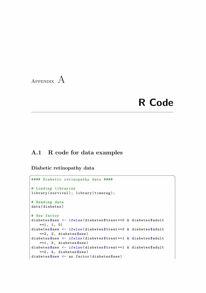
Appendix A
R Code
A.1 R code for data examples
Diabetic retinopathy data� �#### Diabetic retinopathy data ####
# Loading libraries
library(survival); library(timereg);
# Reading data
data(diabetes)
# New factor
diabetes$new <- ifelse(diabetes$treat ==0 & diabetes$adult
==1, 1, 0)
diabetes$new <- ifelse(diabetes$treat ==0 & diabetes$adult
==2, 2, diabetes$new)
diabetes$new <- ifelse(diabetes$treat ==1 & diabetes$adult
==1, 3, diabetes$new)
diabetes$new <- ifelse(diabetes$treat ==1 & diabetes$adult
==2, 4, diabetes$new)
diabetes$new <- as.factor(diabetes$new)
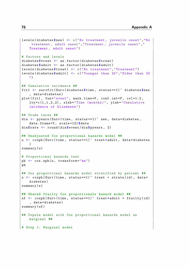
76 Appendix A
levels(diabetes$new) <- c("No treatment , juvenile onset","No
treatment , adult onset","Treatment , juvenile onset","
Treatment , adult onset")
# Factors and levels
diabetes$treat <- as.factor(diabetes$treat)
diabetes$adult <- as.factor(diabetes$adult)
levels(diabetes$treat) <- c("No treatment","Treatment")
levels(diabetes$adult) <- c("Younger than 20","Older than 20
")
## Cumulative incidence ##
fit1 <- survfit(Surv(diabetes$time , status ==1)~ diabetes$new
, data=diabetes)
plot(fit1 , fun="event", mark.time=F, conf.int=F, col=1:2,
lty=c(1,1,2,2), xlab="Time (months)", ylab="Cumulative
incidence of blindness")
## Crude rates ##
dia <- pyears(Surv(time , status ==1)~ new , data=diabetes ,
data.frame=T, scale =12)$data
dia$rate <- round(dia$event/dia$pyears , 2)
## Unadjusted Cox proportional hazards model ##
u <- coxph(Surv(time , status ==1)~ treat*adult , data=diabetes
)
summary(u)
# Proportional hazards test
ph <- cox.zph(u, transform="km")
ph
## Cox proportional hazards model stratified by patient ##
s <- coxph(Surv(time , status ==1)~ treat + strata(id), data=
diabetes)
summary(s)
## Shared frailty Cox proportionals hazard model ##
sf <- coxph(Surv(time , status ==1)~ treat*adult + frailty(id)
, data=diabetes)
summary(sf)
## Copula model with Cox proportional hazards model as
marginal ##
# Step 1: Marginal model
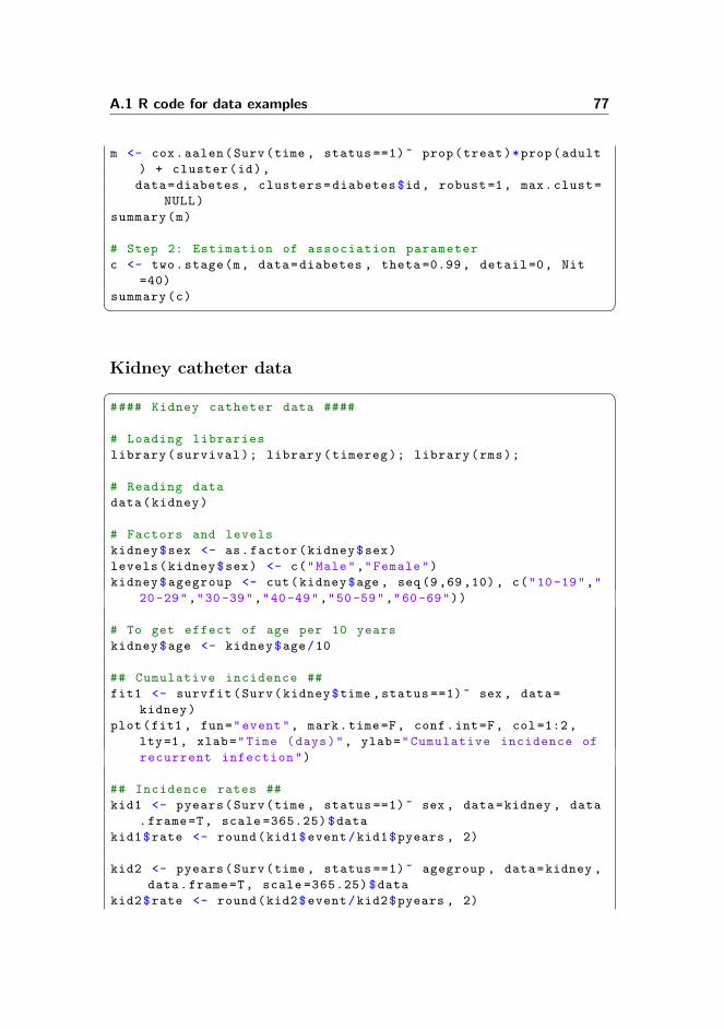
A.1 R code for data examples 77
m <- cox.aalen(Surv(time , status ==1)~ prop(treat)*prop(adult
) + cluster(id),
data=diabetes , clusters=diabetes$id, robust=1, max.clust=
NULL)
summary(m)
# Step 2: Estimation of association parameter
c <- two.stage(m, data=diabetes , theta =0.99 , detail=0, Nit
=40)
summary(c)� �Kidney catheter data� �#### Kidney catheter data ####
# Loading libraries
library(survival); library(timereg); library(rms);
# Reading data
data(kidney)
# Factors and levels
kidney$sex <- as.factor(kidney$sex)
levels(kidney$sex) <- c("Male","Female")
kidney$agegroup <- cut(kidney$age , seq (9 ,69 ,10), c("10-19","
20-29","30-39","40-49","50-59","60-69"))
# To get effect of age per 10 years
kidney$age <- kidney$age/10
## Cumulative incidence ##
fit1 <- survfit(Surv(kidney$time ,status ==1)~ sex , data=
kidney)
plot(fit1 , fun="event", mark.time=F, conf.int=F, col=1:2,
lty=1, xlab="Time (days)", ylab="Cumulative incidence of
recurrent infection")
## Incidence rates ##
kid1 <- pyears(Surv(time , status ==1)~ sex , data=kidney , data
.frame=T, scale =365.25)$data
kid1$rate <- round(kid1$event/kid1$pyears , 2)
kid2 <- pyears(Surv(time , status ==1)~ agegroup , data=kidney ,
data.frame=T, scale =365.25)$data
kid2$rate <- round(kid2$event/kid2$pyears , 2)
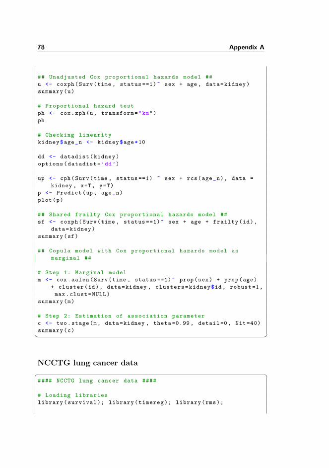
78 Appendix A
## Unadjusted Cox proportional hazards model ##
u <- coxph(Surv(time , status ==1)~ sex + age , data=kidney)
summary(u)
# Proportional hazard test
ph <- cox.zph(u, transform="km")
ph
# Checking linearity
kidney$age_n <- kidney$age*10
dd <- datadist(kidney)
options(datadist=’dd’)
up <- cph(Surv(time , status ==1) ~ sex + rcs(age_n), data =
kidney , x=T, y=T)
p <- Predict(up , age_n)
plot(p)
## Shared frailty Cox proportional hazards model ##
sf <- coxph(Surv(time , status ==1)~ sex + age + frailty(id),
data=kidney)
summary(sf)
## Copula model with Cox proportional hazards model as
marginal ##
# Step 1: Marginal model
m <- cox.aalen(Surv(time , status ==1)~ prop(sex) + prop(age)
+ cluster(id), data=kidney , clusters=kidney$id , robust=1,
max.clust=NULL)
summary(m)
# Step 2: Estimation of association parameter
c <- two.stage(m, data=kidney , theta =0.99 , detail=0, Nit =40)
summary(c)� �NCCTG lung cancer data� �#### NCCTG lung cancer data ####
# Loading libraries
library(survival); library(timereg); library(rms);
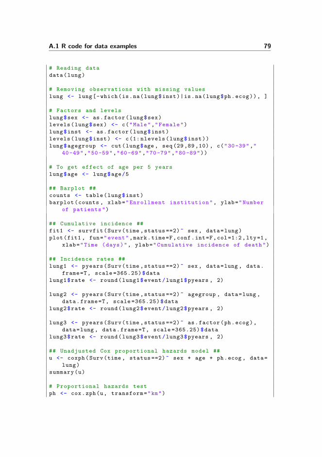
A.1 R code for data examples 79
# Reading data
data(lung)
# Removing observations with missing values
lung <- lung[-which(is.na(lung$inst)|is.na(lung$ph.ecog)), ]
# Factors and levels
lung$sex <- as.factor(lung$sex)
levels(lung$sex) <- c("Male","Female")
lung$inst <- as.factor(lung$inst)
levels(lung$inst) <- c(1: nlevels(lung$inst))
lung$agegroup <- cut(lung$age , seq (29 ,89 ,10), c("30-39","
40-49","50-59","60-69","70-79","80-89"))
# To get effect of age per 5 years
lung$age <- lung$age/5
## Barplot ##
counts <- table(lung$inst)
barplot(counts , xlab="Enrollment institution", ylab="Number
of patients")
## Cumulative incidence ##
fit1 <- survfit(Surv(time ,status ==2)~ sex , data=lung)
plot(fit1 , fun="event",mark.time=F,conf.int=F,col=1:2,lty=1,
xlab="Time (days)", ylab="Cumulative incidence of death")
## Incidence rates ##
lung1 <- pyears(Surv(time ,status ==2)~ sex , data=lung , data.
frame=T, scale =365.25)$data
lung1$rate <- round(lung1$event/lung1$pyears , 2)
lung2 <- pyears(Surv(time ,status ==2)~ agegroup , data=lung ,
data.frame=T, scale =365.25)$data
lung2$rate <- round(lung2$event/lung2$pyears , 2)
lung3 <- pyears(Surv(time ,status ==2)~ as.factor(ph.ecog),
data=lung , data.frame=T, scale =365.25)$data
lung3$rate <- round(lung3$event/lung3$pyears , 2)
## Unadjusted Cox proportional hazards model ##
u <- coxph(Surv(time , status ==2)~ sex + age + ph.ecog , data=
lung)
summary(u)
# Proportional hazards test
ph <- cox.zph(u, transform="km")
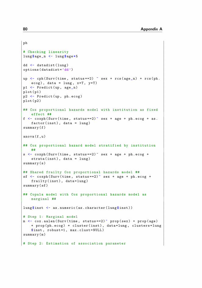
80 Appendix A
ph
# Checking linearity
lung$age_n <- lung$age*5
dd <- datadist(lung)
options(datadist=’dd’)
up <- cph(Surv(time , status ==2) ~ sex + rcs(age_n) + rcs(ph.
ecog), data = lung , x=T, y=T)
p1 <- Predict(up, age_n)
plot(p1)
p2 <- Predict(up, ph.ecog)
plot(p2)
## Cox proportional hazards model with institution as fixed
effect ##
f <- coxph(Surv(time , status ==2)~ sex + age + ph.ecog + as.
factor(inst), data = lung)
summary(f)
anova(f,u)
## Cox proportional hazard model stratified by institution
##
s <- coxph(Surv(time , status ==2)~ sex + age + ph.ecog +
strata(inst), data = lung)
summary(s)
## Shared frailty Cox proportional hazards model ##
sf <- coxph(Surv(time , status ==2)~ sex + age + ph.ecog +
frailty(inst), data=lung)
summary(sf)
## Copula model with Cox proportional hazards model as
marginal ##
lung$inst <- as.numeric(as.character(lung$inst))
# Step 1: Marginal model
m <- cox.aalen(Surv(time , status ==2)~ prop(sex) + prop(age)
+ prop(ph.ecog) + cluster(inst), data=lung , clusters=lung
$inst , robust=1, max.clust=NULL)
summary(m)
# Step 2: Estimation of association parameter
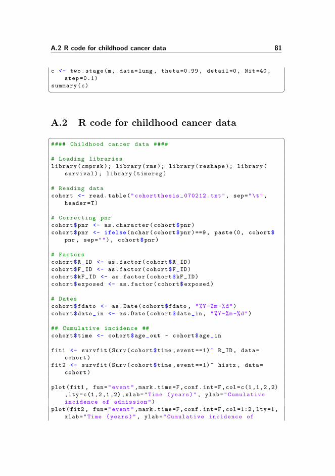
A.2 R code for childhood cancer data 81
c <- two.stage(m, data=lung , theta =0.99 , detail=0, Nit=40,
step =0.1)
summary(c)� �A.2 R code for childhood cancer data� �#### Childhood cancer data ####
# Loading libraries
library(cmprsk); library(rms); library(reshape); library(
survival); library(timereg)
# Reading data
cohort <- read.table("cohortthesis_070212. txt", sep="\t",
header=T)
# Correcting pnr
cohort$pnr <- as.character(cohort$pnr)
cohort$pnr <- ifelse(nchar(cohort$pnr)==9, paste(0, cohort$
pnr , sep=""), cohort$pnr)
# Factors
cohort$R_ID <- as.factor(cohort$R_ID)
cohort$F_ID <- as.factor(cohort$F_ID)
cohort$kF_ID <- as.factor(cohort$kF_ID)
cohort$exposed <- as.factor(cohort$exposed)
# Dates
cohort$fdato <- as.Date(cohort$fdato , "%Y-%m-%d")
cohort$date_in <- as.Date(cohort$date_in, "%Y-%m-%d")
## Cumulative incidence ##
cohort$time <- cohort$age_out - cohort$age_in
fit1 <- survfit(Surv(cohort$time ,event ==1)~ R_ID, data=
cohort)
fit2 <- survfit(Surv(cohort$time ,event ==1)~ histx , data=
cohort)
plot(fit1 , fun="event",mark.time=F,conf.int=F,col=c(1,1,2,2)
,lty=c(1,2,1,2),xlab="Time (years)", ylab="Cumulative
incidence of admission")
plot(fit2 , fun="event",mark.time=F,conf.int=F,col=1:2,lty=1,
xlab="Time (years)", ylab="Cumulative incidence of
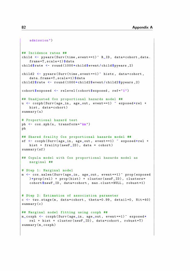
82 Appendix A
admission")
## Incidence rates ##
child <- pyears(Surv(time ,event ==1)~ R_ID , data=cohort ,data.
frame=T,scale =1)$data
child$rate <- round (1000*child$event/child$pyears ,2)
child2 <- pyears(Surv(time ,event ==1)~ histx , data=cohort ,
data.frame=T,scale =1)$data
child2$rate <- round (1000*child2$event/child2$pyears ,2)
cohort$exposed <- relevel(cohort$exposed , ref="1")
## Unadjusted Cox proportional hazards model ##
u <- coxph(Surv(age_in , age_out , event ==1) ~ exposed*rel +
hist , data=cohort)
summary(u)
# Proportional hazard test
ph <- cox.zph(u, transform="km")
ph
## Shared frailty Cox proportional hazards model ##
sf <- coxph(Surv(age_in, age_out , event ==1) ~ exposed*rel +
hist + frailty(newF_ID), data = cohort)
summary(sf)
## Copula model with Cox proportional hazards model as
marginal ##
# Step 1: Marginal model
m <- cox.aalen(Surv(age_in , age_out , event ==1)~ prop(exposed
)*prop(rel) + prop(hist) + cluster(newF_ID), clusters=
cohort$newF_ID, data=cohort , max.clust=NULL , robust =1)
# Step 2: Estimation of association parameter
c <- two.stage(m, data=cohort , theta =0.99 , detail=0, Nit =40)
summary(c)
## Marginal model fitting using coxph ##
m_coxph <- coxph(Surv(age_in , age_out , event ==1)~ exposed*
rel + hist + cluster(newF_ID), data=cohort , robust=T)
summary(m_coxph)
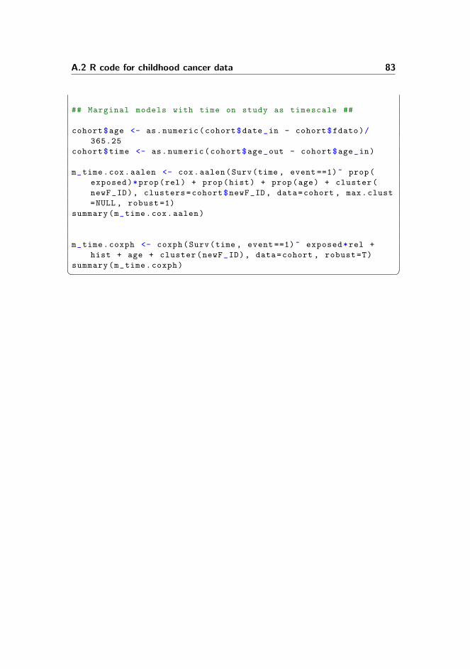
A.2 R code for childhood cancer data 83
## Marginal models with time on study as timescale ##
cohort$age <- as.numeric(cohort$date_in - cohort$fdato)/
365.25
cohort$time <- as.numeric(cohort$age_out - cohort$age_in)
m_time.cox.aalen <- cox.aalen(Surv(time , event ==1)~ prop(
exposed)*prop(rel) + prop(hist) + prop(age) + cluster(
newF_ID), clusters=cohort$newF_ID, data=cohort , max.clust
=NULL , robust =1)
summary(m_time.cox.aalen)
m_time.coxph <- coxph(Surv(time , event ==1)~ exposed*rel +
hist + age + cluster(newF_ID), data=cohort , robust=T)
summary(m_time.coxph)� �

84
Appendix B
Additional Results
B.1 Kidney catheter data
Here, additional results for the kidney catheter data are presented. The statis-tical analyses presented in Chapter 4 have been repeated without the patientwith identification number 21. The results if these analyses are summarised inTable B.1.
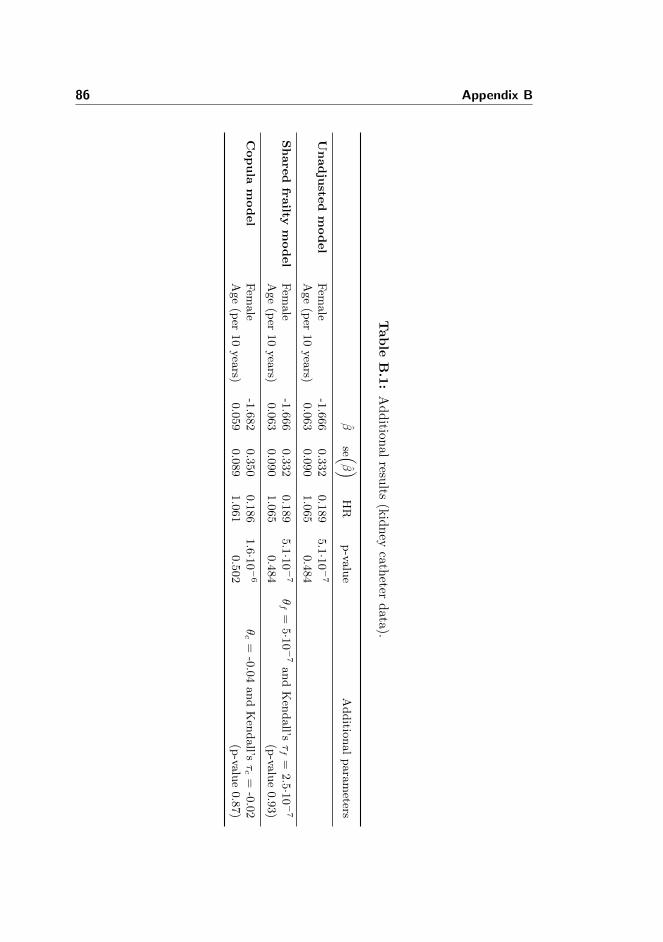
86 Appendix B
Tab
leB
.1:
Ad
dition
alresu
lts(k
idn
eyca
theter
data
).
βse (
β )HR
p-va
lue
Additio
nalparameters
Unadju
sted
model
Fem
ale
-1.666
0.332
0.189
5.1·1
0−7
Age(per
10years)
0.063
0.090
1.065
0.484
Share
dfra
iltym
odel
Fem
ale
-1.666
0.332
0.189
5.1·1
0−7
θf=
5·10−7andKen
dall’s
τf=
2.5·1
0−7
Age(per
10years)
0.063
0.090
1.065
0.484
(p-va
lue0.93)
Copula
model
Fem
ale
-1.682
0.350
0.186
1.6·1
0−6
θc=
-0.04andKen
dall’s
τc=
-0.02
Age(per
10years)
0.059
0.089
1.061
0.502
(p-va
lue0.87)

Bibliography
[1] Elisabeth W. Andersen. Composite likelihood and two-stage estimation infamily studies. Biostatistics, 5:15–30, 2004.
[2] Elisabeth W. Andersen. Two-stage estimation in copula models used infamily studies. Lifetime Data Analysis, 11:333–350, 2005.
[3] Karen J. Bandeen-Roche and Liang K.-Y. Modelling failure-time associa-tions in data with multiple levels of clustering. Biometrika, 83:29–39, 1996.
[4] David Buchbinder, Jacqueline Casillas, Kevin R. Krull, Pam Goodman,Wendy Leisenring, Christopher Recktilis, Melissa A. Alderfer, Leslie L. Ro-bison, Gregory T. Armstrong, Alicia Kunin-Batson, Margaret Stuber, andLonnie K. Zelzter. Psychological outcomes of siblings of cancer survivors:A report from the Childhood Cancer Survior Study. Psycho-Oncology,20:1259–1268, 2011.
[5] D.G. Clayton. A model for association in bivariate life tables and its ap-plication in epidemiological studies of familial tendency in chronic diseaseincidence. Biometrika, 65:141–151, 1978.
[6] David R. Cox. Regression models and life-tables (with discussion). Journalof the Royal Statistical Society, Series B, 34:187–220, 1972.
[7] Luc Duchateau and Paul Janssen. The Frailty Model. Springer, 2008.
[8] Bradley Efron. The efficiency of Cox’s likelihood function for censored data.Journal of the American Statistical Association, 72:557–565, 1977.
[9] Thomas R. Fleming and David P. Harrington. Counting Processes andSurvival Analysis. John Wiley & Sons, Inc., 1991.
88 BIBLIOGRAPHY
[10] Christian Genest and Jock MacKay. The joy of copulas: Bivariate dis-tributions with uniform margins. The American Statistician, 40:280–283,1986.
[11] Christian Genest and R. Jock MacKay. Copules achimediennes et famillesde lois bidimensionnelles dont les marges sont donnees. The CanadianJournal of Statistics, 14:145–159, 1986.
[12] Richard D. Gill. Understanding Cox’s regression model: A martingaleapproach. Journal of the American Statistical Association, 79:441–447,1984.
[13] Marianne L. Gjerstorff. The Danish Cancer Registry. Scandinavian Journalof Public Health, 39:42–45, 2011.
[14] David V. Glidden. Checking the adequacy of the gamma frailty model formultivariate failure times. Biometrika, 86:381–393, 1999.
[15] David V. Glidden. A two-stage estimator of the dependence parameter forthe Clayton-Oakes model. Lifetime Data Analysis, 6:141–156, 2000.
[16] David V. Glidden and Steven G. Self. Semiparametric likelihood estima-tion in the Clayton-Oakes failure time model. Scandinavian Journal ofStatistics, 26:363–372, 1999.
[17] Klara Goethals, Paul Jannsen, and Luc Duchateau. Frailty models andcopulas: Similarities and differences. Journal of Applied Statistics, 35:1071–1079, 2008.
[18] Lynn R. Goldin, Ruth M. Pfeiffer, Gloria Gridley, Mitchell H. Gail, XinjunLi, Lene Mellemkjaer, Jørgen H. Olsen, Kari Hemminki, and Martha S.Linet. Familial aggregation of Hodgkin lymphoma and related tumors.Cancer, 100:1902–1908, 2004.
[19] Lynn R. Goldin, Ruth M. Pfeiffer, and Kari Hemminki. Familial risk oflymphoproliferative tumors in families of patients with chronic lympho-cytic leukemia: Results from the Swedish family-cancer database. Blood,104:1850–1854, 2004.
[20] Patricia M. Grambsch and Terry M. Therneau. Proportional hazards testsand diagnostics based on weighted residuals. Biometrika, 81:515–526, 1994.
[21] James G. Gurney, Kevin R. Krull, Nina Kadan-Lottick, H. Stacy Nicholson,Paul C. Nathan, Brad Zebrack, Jean M. Tersak, and Kirsten K. Ness.Social outcomes in the Childhood Cancer Survior Study cohort. Journal ofClinical Oncology, 27:2390–2395, 2009.
BIBLIOGRAPHY 89
[22] Philip Hougaard. Frailty models for survival data. Lifetime Data Analysis,1:255–273, 1995.
[23] Philip Hougaard. Analysis of Multivariate Survival Data. Springer, 2000.
[24] Philip Hougaard, Bent Harvald, and Niels V. Holm. Measuring similari-ties between the lifetimes of adult Danish twins born between 1881-1930.Journal of the American Statistical Association, 87:17–24, 1992.
[25] William J. Huster, Ron Brookmeyer, and Steven G. Self. Modelling pairedsurvival data with covariates. Biometrics, 45:145–156, 1989.
[26] John P. Klein. Semiparametric estimation of random effects using the Coxmodel based on the EM algorithm. Biometrics, 48:795–806, 1992.
[27] David G. Kleinbaum and Mitchel Klein. Survival Analysis - A Self-LearningText. Springer, second edition, 2005.
[28] Edward L. Korn, Barry I. Graubard, and Douglas Midthune. Time-to-event analysis of longitudinal follow-up of a survey: Choice of time-scale.American Journal of Epidemiology, 145:72–80, 1997.
[29] Elisa T. Lee and John W. Wang. Statistical Methods for Survival DataAnalysis. John Wiley & Sons, Inc., third edition, 2003.
[30] E.W. Lee, L.J. Wei, and D.A. Amato. Cox-type regression analysis for largenumber of small groups of correlated failure time observations. In J.P. Kleinand P.K. Goel, editors, Survival Analysis, State of the Art, pages 237–247.Kluwer, 1992.
[31] Stuart R. Lipsitz, Keith B.G. Dear, and Lueping Zhao. Jackknife estima-tors of variance for parameter estimates from estimating equations withapplications to clustered survival data. Biometrics, 50:842–846, 1994.
[32] Stuart R. Lipsitz and Michael Parzen. A jackknife estimator of variance forCox regression for correlated survival data. Biometrics, 52:291–298, 1996.
[33] C.L. Loprinzi, J.A. Laurie, H.S. Wieand, J.E. Krook, P.J. Novotny, J.W.Kugler, J. Bartel, M. Law, M. Bateman, and N.E. Klatt. Prospectiveevaluation of prognostic variables from patient-completed questionnaires.North Central Cancer Treatment Group. Journal of Clinical Oncology,12:601–607, 1994.
[34] Lasse W. Lund, Kjeld Schmiegelow, Catherine Rechnitzer, and ChristofferJohansen. A systematic review of studies on psychological late effects ofchildhood cancer: Structures of society and methodological pitfalls maychallenge conclusions. Pediatric Blood & Cancer, 56:532–543, 2011.
90 BIBLIOGRAPHY
[35] Wendy Mack, Bryan Langholz, and Duncan C. Thomas. Survival models forfamilial aggregation of cancer. Environmental Health Perspectives, 87:27–35, 1990.
[36] Torben Martinussen and Thomas H. Scheike. Dynamic Regression Modelsfor Survival Data. Springer, 2006.
[37] C.A. McGilchrist and C.W. Aisbett. Regression with frailty in survivalanalysis. Biometrics, 47:461–466, 1991.
[38] Tron A. Moger, Marion Haugen, Benjamin H.K. Yip, Hakon K. Gjessing,and Ørnulf Borgan. A hierarchical frailty model applied to two generationmelanoma data. Lifetime Data Analysis, 17:445–460, 2011.
[39] Douglas M. Montgomery. Design and Analysis of Experiments. John Wiley& Sons, Inc., seventh edition, 2009.
[40] Ole Mors, Gurli P. Perto, and Preben B. Mortensen. The Danish Psychi-atric Central Research Register. Scandinavian Journal of Public Health,39:54–57, 2011.
[41] Roger B. Nelsen. An Introduction to Copulas. Springer, second edition,2006.
[42] David Oakes. A model for association in bivariate survival data. Journalof the Royal Statistical Society, Series B, 44:414–422, 1982.
[43] David Oakes. Bivariate survival models induced by frailties. Journal of theAmerican Statistical Association, 84:487–493, 1989.
[44] Carsten B. Pedersen. The Danish Civil Registration System. ScandinavianJournal of Public Health, 39:22–25, 2011.
[45] Carsten B. Pedersen, Heine Gøtzsche, Jørgen Ø. Møller, and Preben B.Mortensen. The Danish Civil Registration System. Danish Medical Bul-letin, 53:441–449, 2006.
[46] Jørgen Holm Petersen. A additive frailty model for correlated life times.Biometrics, 54:646–661, 1998.
[47] R.M. Pfeiffer, L.R. Goldin, N. Chatterjee, S. Daugherty, K. Hemminki,D. Pee, L.I. X, and M.H. Gail. Methods for testing familial aggregation ofdiseases in population-based samples: Application to Hodgkin lymphomain Swedish registry data. Annals of Human Genetics, 68:498–508, 2004.
[48] R Development Core Team. R: A Language and Environment for Statisti-cal Computing. R Foundation for Statistical Computing, Vienna, Austria,2011. ISBN 3-900051-07-0.
BIBLIOGRAPHY 91
[49] Joanna H. Shih and Thomas A. Louis. Assessing gamma frailty models forclustered failure time data. Lifetime Data Analysis, 1:205–220, 1995a.
[50] Joanna H. Shih and Thomas A. Louis. Inferences on the association param-eter in copula models for bivariate survival data. Biometrics, 51:1384–1399,1995b.
[51] Charles F. Spiekerman and D.Y. Lin. Marginal regression models for mul-tivariate failure time data. Journal of the American Statistical Association,93:1164–1175, 1998.
[52] Terry M. Therneau and Patricia M. Grambsch. Modeling Survival Data -Extending the Cox Model. Springer, 2000.
[53] Terry M. Therneau, Patricia M. Grambsch, and V. Shane Pankratz. Penal-ized survival models and frailty. Journal of Computational and GraphicalStatistics, 12:156–175, 2003.
[54] Anne C.M. Thiebaut and Jacques Benichou. Choice of time-sclae in Cox’smodel analysis of epidemiologic cohort data: A simulation study. Statisticsin Medicine, 23:3803–3820, 2004.
[55] Pravin K. Trivedi and David M. Zimmer. Copula Modeling: An Introduc-tion for Practitioners. Now Pub, 2007.
[56] L.J. Wei, D.Y. Lin, and L. Weissfeld. Regression analysis of multivariateincomplete failure time data by modeling marginal distributions. Journalof the American Statistical Association, 84:1065–1073, 1989.
[57] Halbert White. Maximum likelihood estimation of misspecified models.Econometrica, 50:1–25, 1982.
[58] Andreas Wienke. Frailty Models in Survival Analysis. Chapmann & Hall,2011.
[59] Anatoli I. Yashin, James W. Vaupel, and Ivan A. Iachine. Correlated indi-vidual frailty: An advantageous approach to survival analysis of bivariatedata. Mathematical Population Studies, 5:145–159, 1995.
[60] Lonnie K. Zeltzer, Christopher Recklitis, David Buchbinder, Bradley Ze-brack, Jacqueline Casillas, Jennie C.I. Tsao, Qian Lu, and Kevin Krull.Psychological status in childhood cancer survivors: A report from theChildhood Cancer Survior Study. Journal of Clinical Oncology, 27:2396–2404, 2009.
![Sarika Arora, MD, Metabolic effects of obesity: A review · obesity, as has been demonstrated by familial aggregation, twin and adoption studies[1,2]. Estimates for a genetic basis](https://img.pdfslide.us/doc/110x75/5f8d11da7c3bc0232b547398/sarika-arora-md-metabolic-effects-of-obesity-a-review-obesity-as-has-been-demonstrated.jpg)