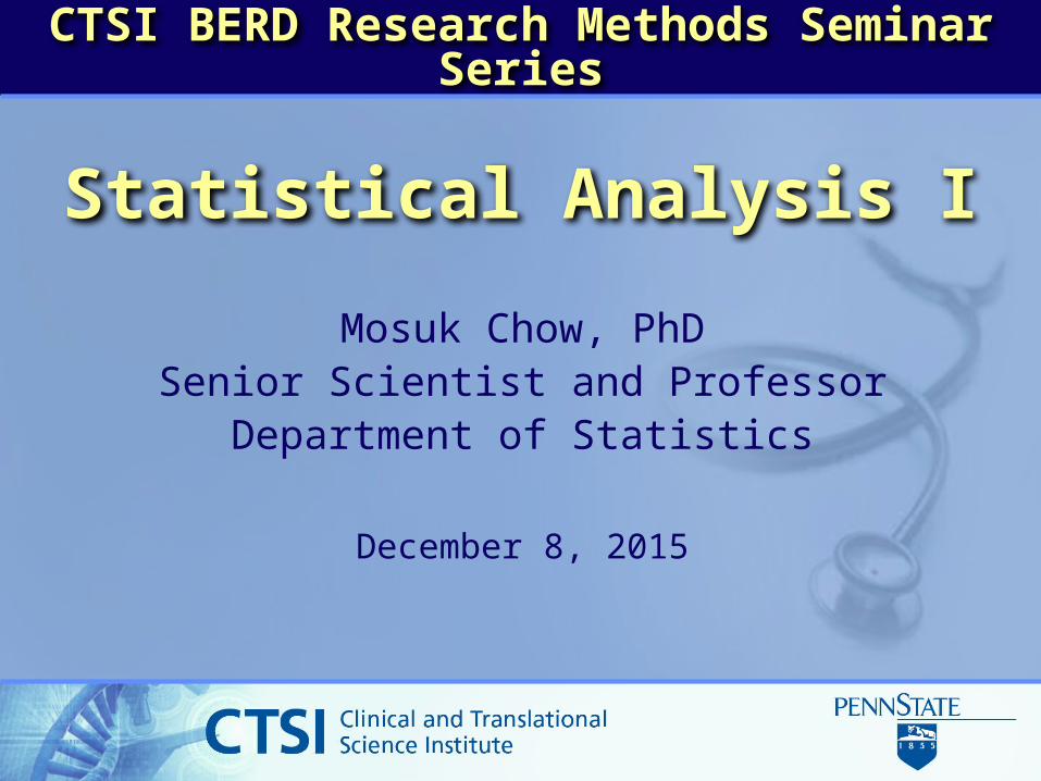
Statistical Analysis I

Mosuk Chow, PhDSenior Scientist and Professor

Department of Statistics

December 8, 2015

CTSI BERD Research Methods Seminar Series

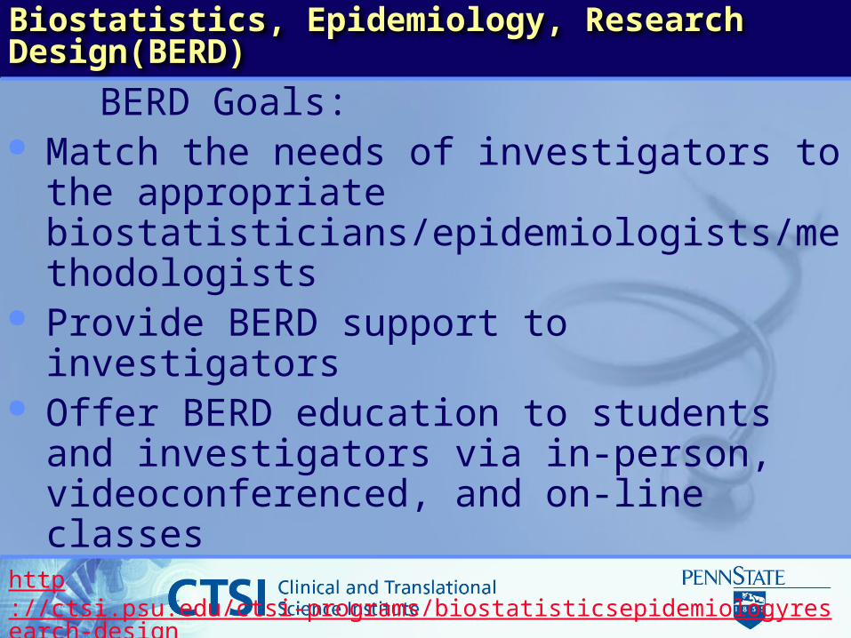
Biostatistics, Epidemiology, Research Design(BERD)

BERD Goals: Match the needs of investigators to the

appropriate biostatisticians/epidemiologists/methodologists

Provide BERD support to investigators Offer BERD education to students and

investigators via in-person, videoconferenced, and on-line classes

http://ctsi.psu.edu/ctsi-programs/biostatisticsepidemiologyresearch-design/

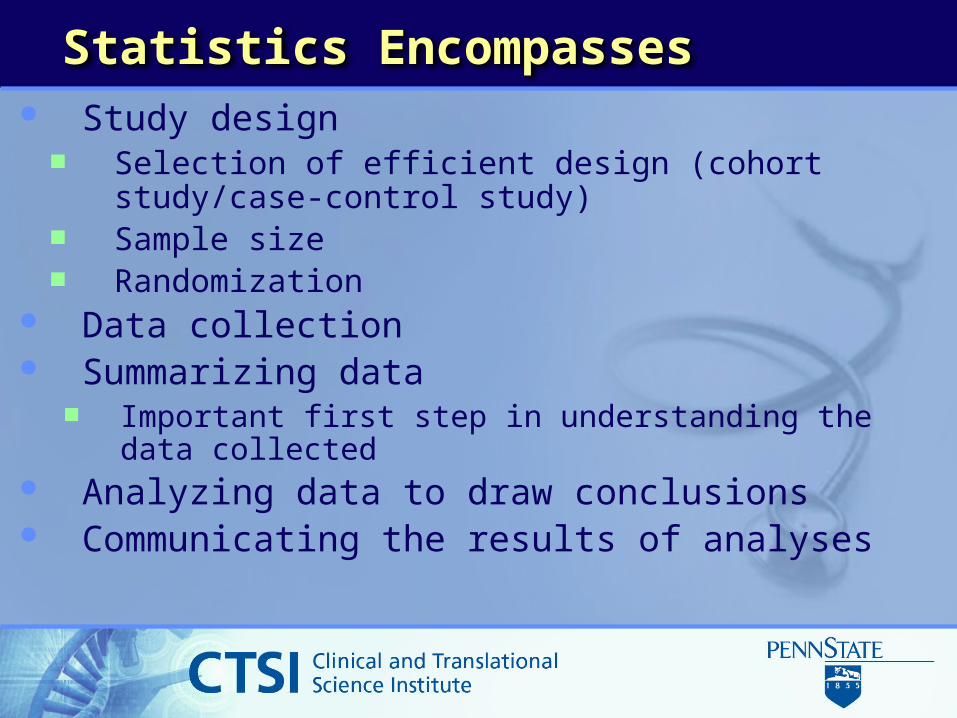
Statistics Encompasses Study design

Selection of efficient design (cohort study/case-control study)

Sample size Randomization

Data collection Summarizing data

Important first step in understanding the data collected Analyzing data to draw conclusions Communicating the results of analyses

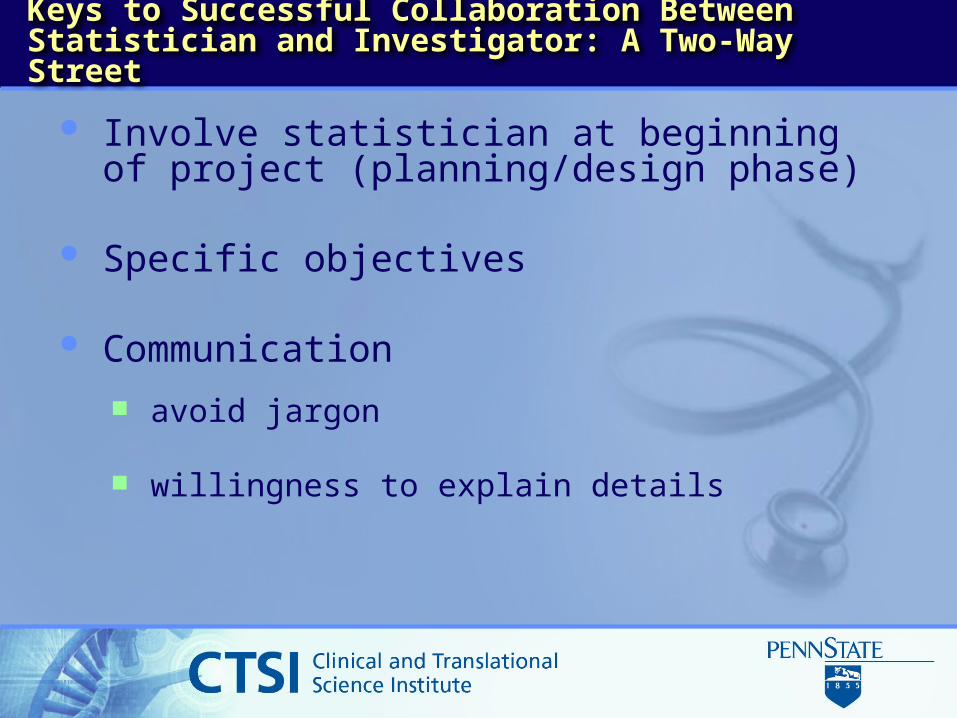
Keys to Successful Collaboration Between Statistician and Investigator: A Two-Way Street

Involve statistician at beginning of project (planning/design phase)

Specific objectives

Communication avoid jargon

willingness to explain details

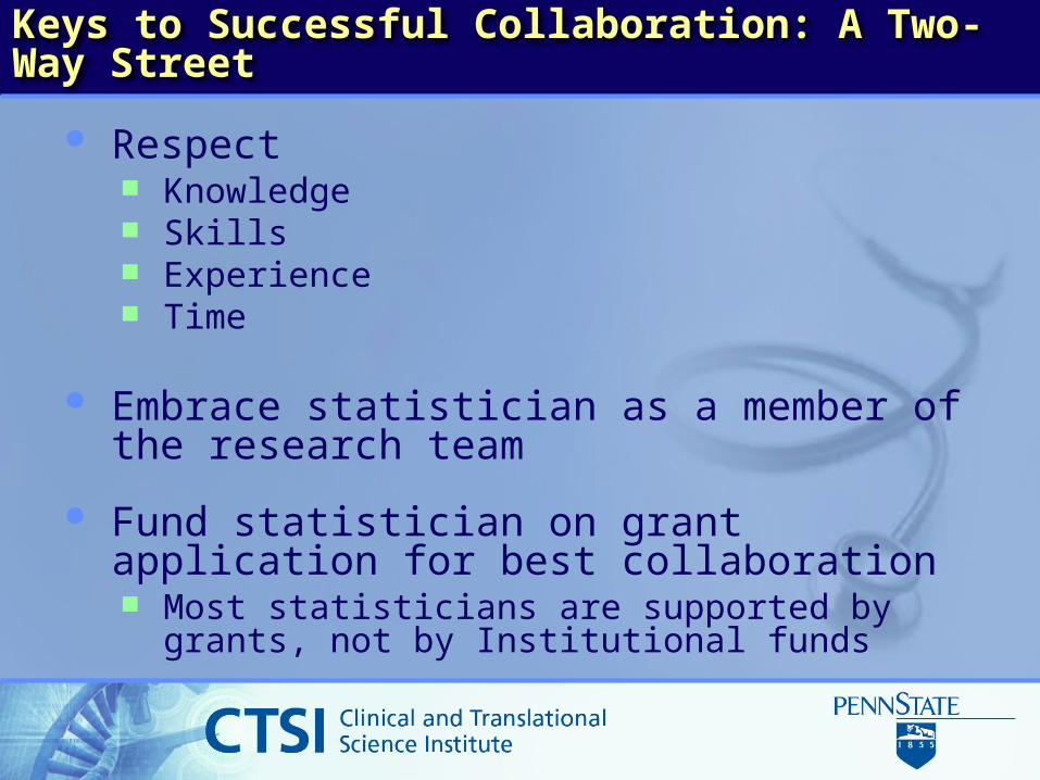
Keys to Successful Collaboration: A Two-Way Street

Respect Knowledge Skills Experience Time

Embrace statistician as a member of the research team

Fund statistician on grant application for best collaboration Most statisticians are supported by grants, not by

Institutional funds

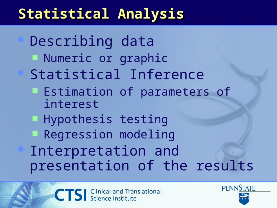
Statistical Analysis

Describing data Numeric or graphic

Statistical Inference Estimation of parameters of interest Hypothesis testing Regression modeling

Interpretation and presentation of the results

Describing data: Basic Terms

Measurement – assignment of a number to a characteristic of an object or event

Data – collection of measurements Sample – collected data Population – all possible data Variable – a property or characteristic of the

population/sample – e.g., gender, weight, blood pressure.

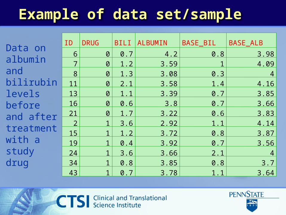
Example of data set/sample

Data on albumin and bilirubin levels before and after treatment with a study drug

ID DRUG BILI ALBUMIN BASE_BIL BASE_ALB6 0 0.7 4.2 0.8 3.987 0 1.2 3.59 1 4.098 0 1.3 3.08 0.3 4

11 0 2.1 3.58 1.4 4.1613 0 1.1 3.39 0.7 3.8516 0 0.6 3.8 0.7 3.6621 0 1.7 3.22 0.6 3.83

2 1 3.6 2.92 1.1 4.1415 1 1.2 3.72 0.8 3.8719 1 0.4 3.92 0.7 3.5624 1 3.6 3.66 2.1 434 1 0.8 3.85 0.8 3.743 1 0.7 3.78 1.1 3.64

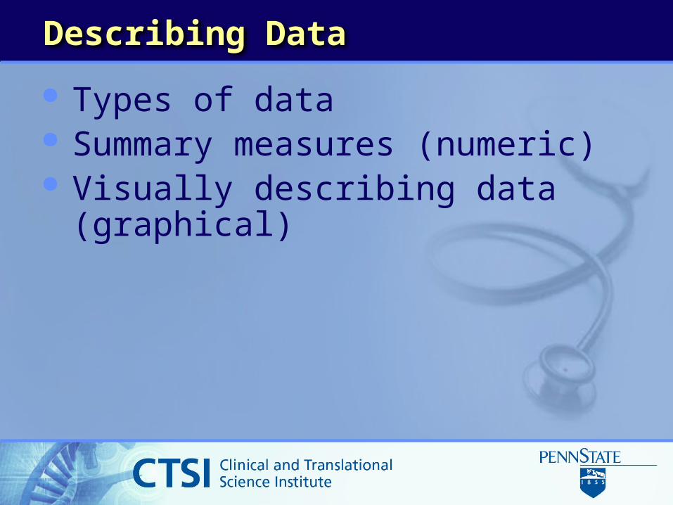
Describing Data

Types of data Summary measures (numeric) Visually describing data (graphical)

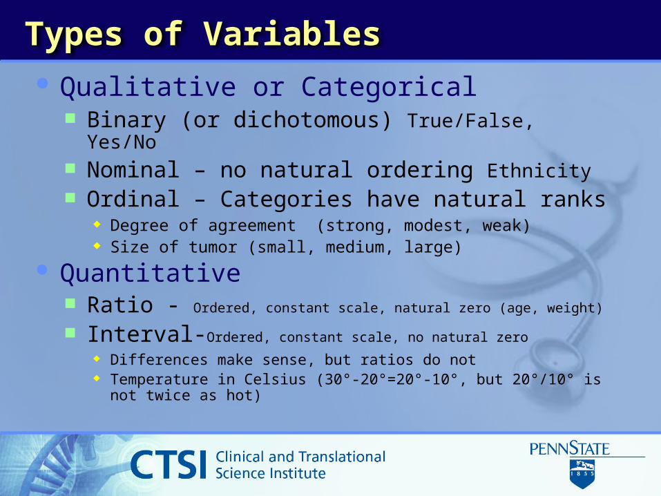
Types of Variables

Qualitative or Categorical Binary (or dichotomous) True/False, Yes/No Nominal – no natural ordering Ethnicity Ordinal – Categories have natural ranks

Degree of agreement (strong, modest, weak) Size of tumor (small, medium, large)

Quantitative Ratio - Ordered, constant scale, natural zero (age, weight)

Interval-Ordered, constant scale, no natural zero

Differences make sense, but ratios do not Temperature in Celsius (30°-20°=20°-10°, but 20°/10° is not

twice as hot)

Types of Measurements for Quantitative Variables

Continuous: Weight, Height, Age Discrete: a countable number of values

The number of births, Age in years Likert scale: “agree”, “strongly agree”, etc.

Somewhere between ordinal and discrete Scales with <= 4 possibilities are usually

considered to be ordinal. Scales with >=7 possibilities are usually considered

to be discrete.

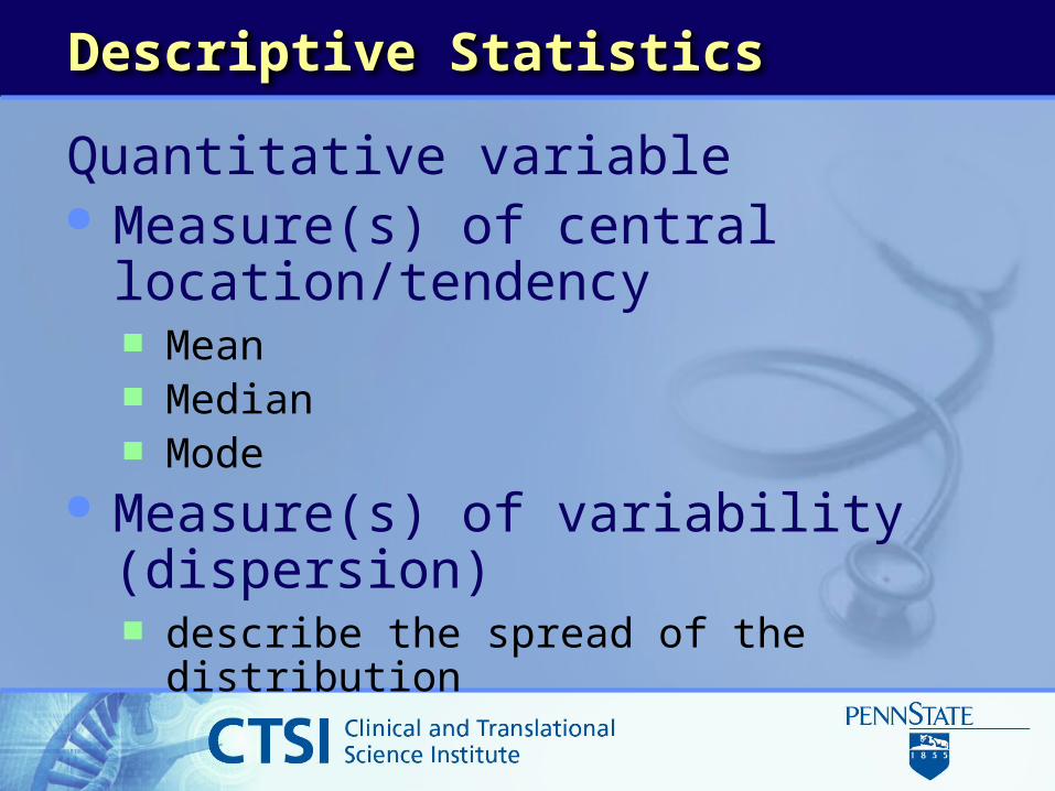
Descriptive Statistics

Quantitative variable Measure(s) of central location/tendency

Mean Median Mode

Measure(s) of variability (dispersion) describe the spread of the distribution

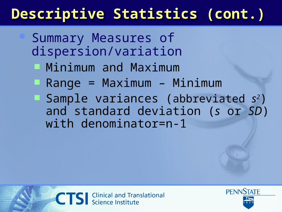
Summary Measures of dispersion/variation Minimum and Maximum Range = Maximum – Minimum Sample variances (abbreviated s2) and

standard deviation (s or SD) with denominator=n-1

Descriptive Statistics (cont.)

Other Measures of Variation Interquartile range (IQR): 75th percentile – 25th percentile MAD: median absolute deviation CV: Coefficient of variation

Ratio of SD over sample mean Measure relative variability Independent of measurement units Useful for comparing two or more sets of data

Tell whole story of data, detect outliers Histogram Stem and Leaf Plot Box Plot

Describing data graphically

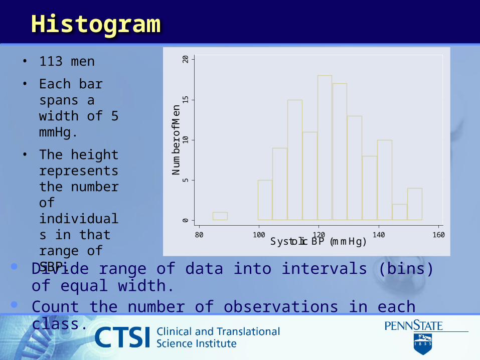
Histogram

Divide range of data into intervals (bins) of equal width. Count the number of observations in each class.

05

1015

20N

um

be

r o

f M

en

80 100 120 140 160Systolic BP (mmHg)

• 113 men

• Each bar spans a width of 5 mmHg.

• The height represents the number of individuals in that range of SBP.

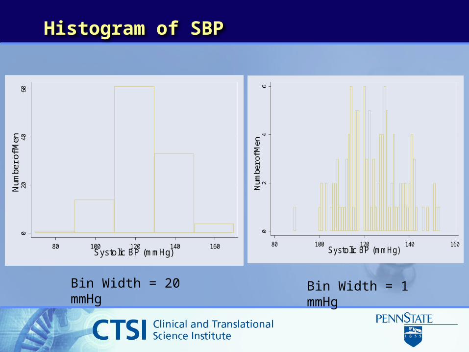
Histogram of SBP0

2040

60N

umbe

r of

Men

80 100 120 140 160Systolic BP (mmHg)

Bin Width = 20 mmHg

02

46

Num

ber o

f Men

80 100 120 140 160Systolic BP (mmHg)

Bin Width = 1 mmHg

Stem and Leaf Plot

Provides a good summary of data structure Easy to construct and much less prone to error

than the tally method of finding a histogram

2 8 8 9

3 0 1 1 1 2 3 3 4 4 5 5 5 5 6 6 6 7 7 7 7 8 9 94 0 0 1 1 1 1 1 2 2 3 3 3 4 4 4 4 5 5 5 6 7 7 8 95 0 1 1 2 3 4

“stem”: the first digit or digits of the number.“leaf” : the trailing digit.

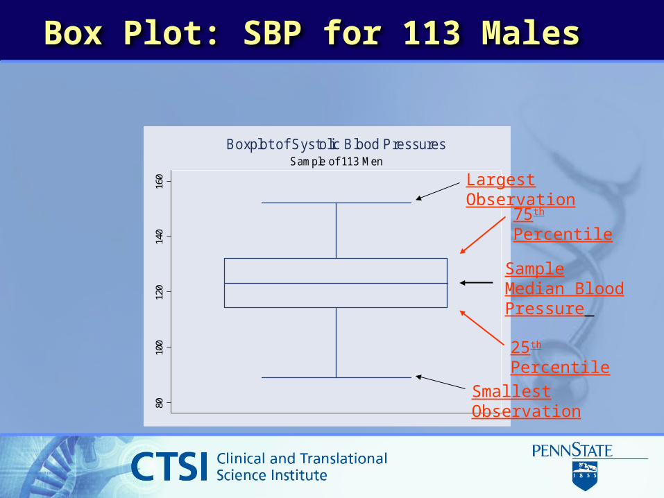
Box Plot: SBP for 113 Males

8010

012

014

016

0Sample of 113 Men

Boxplot of Systolic Blood Pressures

Sample Median Blood Pressure

75th Percentile

25th Percentile

Largest Observation

Smallest Observation

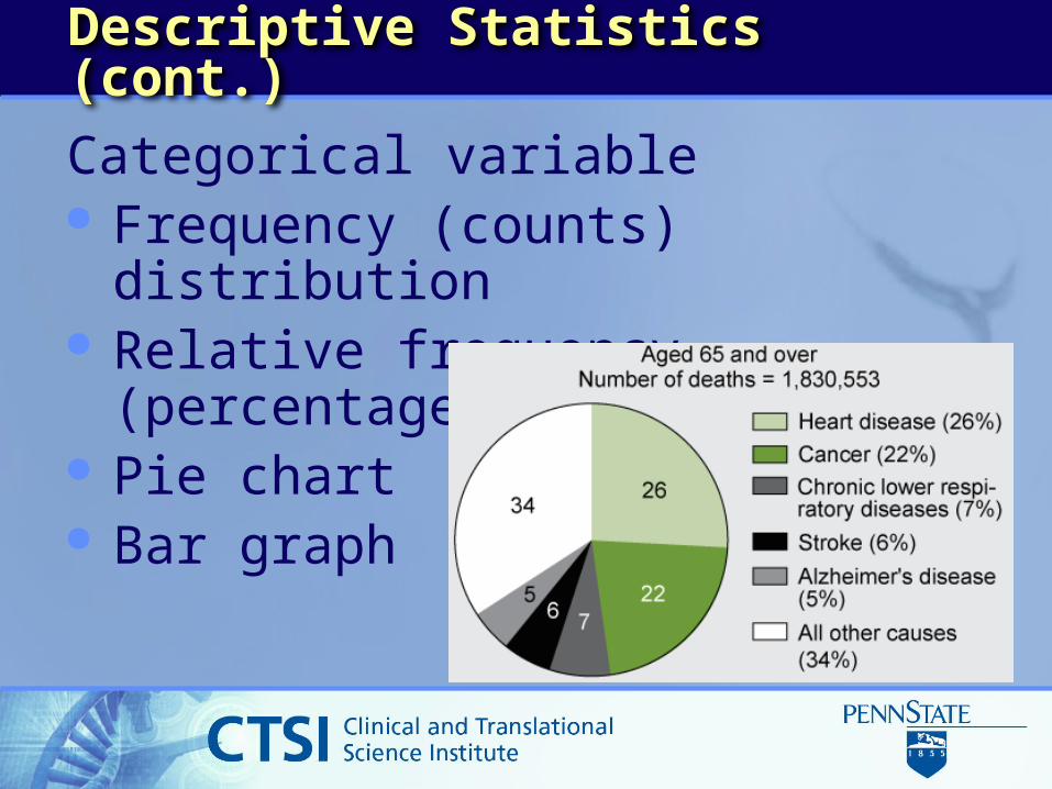
Descriptive Statistics (cont.)

Categorical variable Frequency (counts) distribution Relative frequency (percentages) Pie chart Bar graph

Describe relationship between two variables

One quantitative and one categorical Descriptive statistics within each category Side by side boxplots/histogramsBoth quantitative Scatter plotBoth categorical Contingency table

A process of making inference (an estimate, prediction, or decision) about a population (parameters) based on a sample (statistics) drawn from that population.

Statistical Inference0

.1.2

.3.4

Perc

enta

ge

80 100 120 140 160 180Systolic BP (mmHg)

05

1015

20N

um

be

r o

f M

en

80 100 120 140 160Systolic BP (mmHg)

Statistics (Vary from sample to sample)

Parameters (Fixed, unknown)

Population

Sample

Inference

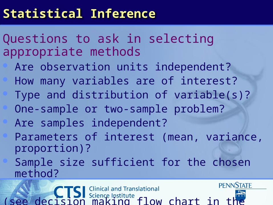
Statistical Inference

Questions to ask in selecting appropriate methods Are observation units independent? How many variables are of interest? Type and distribution of variable(s)? One-sample or two-sample problem? Are samples independent? Parameters of interest (mean, variance, proportion)? Sample size sufficient for the chosen method?

(see decision making flow chart in the handout)

Estimation of population mean

We don’t know the population mean μ but would like to estimate it.

We draw a sample from the population. We calculate the sample mean X. How close is X to μ? Statistical theory will tell us how close X is to μ. Statistical inference is the process of trying to

draw conclusions about the population from the sample.

Key Statistical Concept

Question: How close is the sample mean to the population mean?

Statistical Inference for sample mean Sample mean will change from sample to

sample We need a statistical model to quantify the

distribution of sample means (Sampling distribution)

Sometimes, need “normal distribution” for the population data

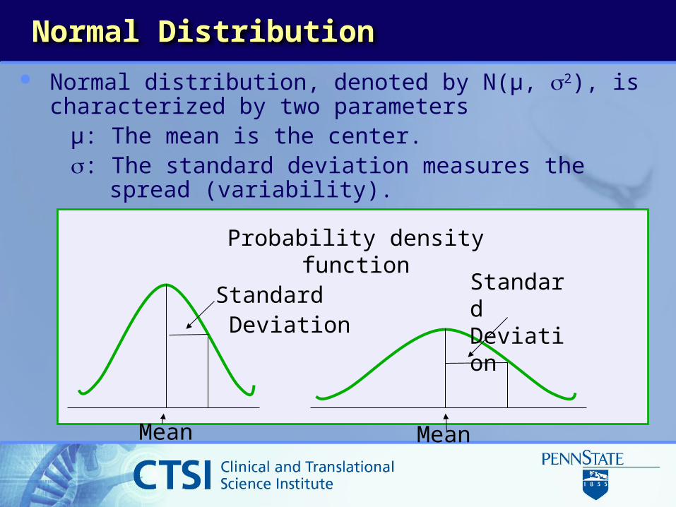
Normal Distribution

Normal distribution, denoted by N(µ, 2), is characterized by two parameters

µ: The mean is the center. : The standard deviation measures the spread (variability).

Mean

Standard Deviation

Standard Deviation

Mean

Probability density function

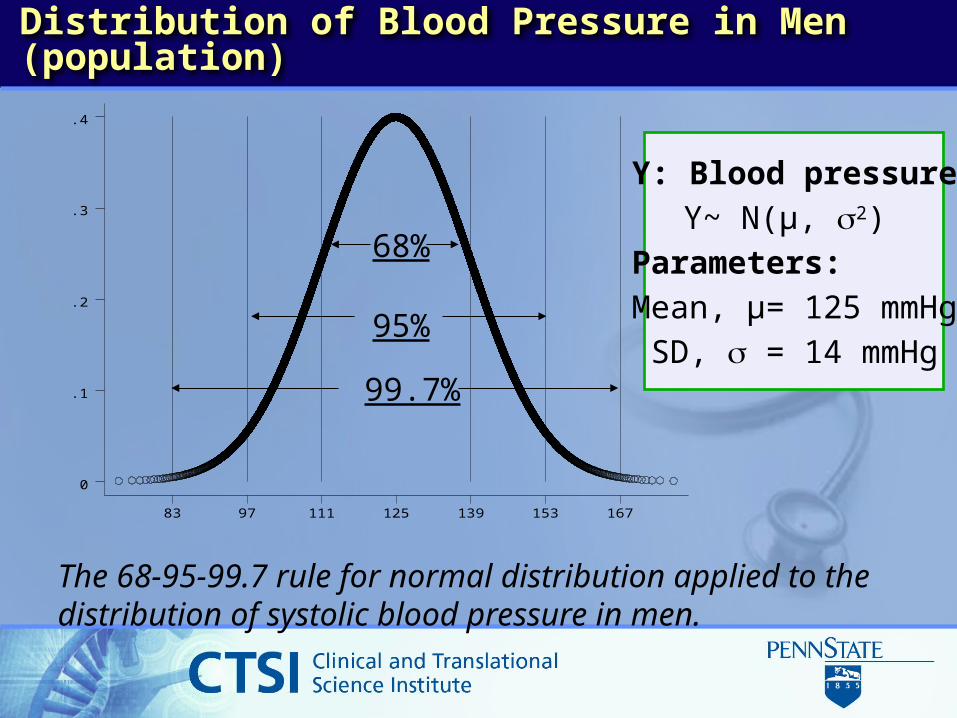
Distribution of Blood Pressure in Men (population)

Y: Blood pressureY~ N(µ, 2)

Parameters:Mean, µ= 125 mmHg

SD, = 14 mmHg

83 97 111 125 139 153 167

0

.1

.2

.3

.4

99.7%

95%

68%

The 68-95-99.7 rule for normal distribution applied to the distribution of systolic blood pressure in men.

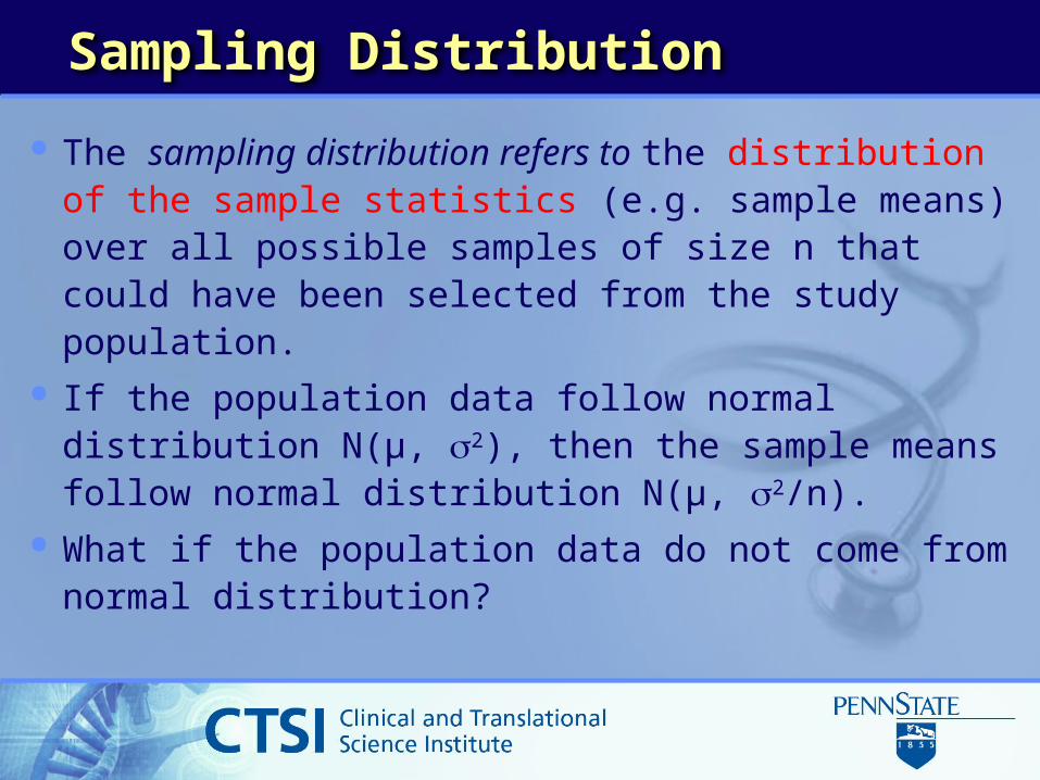
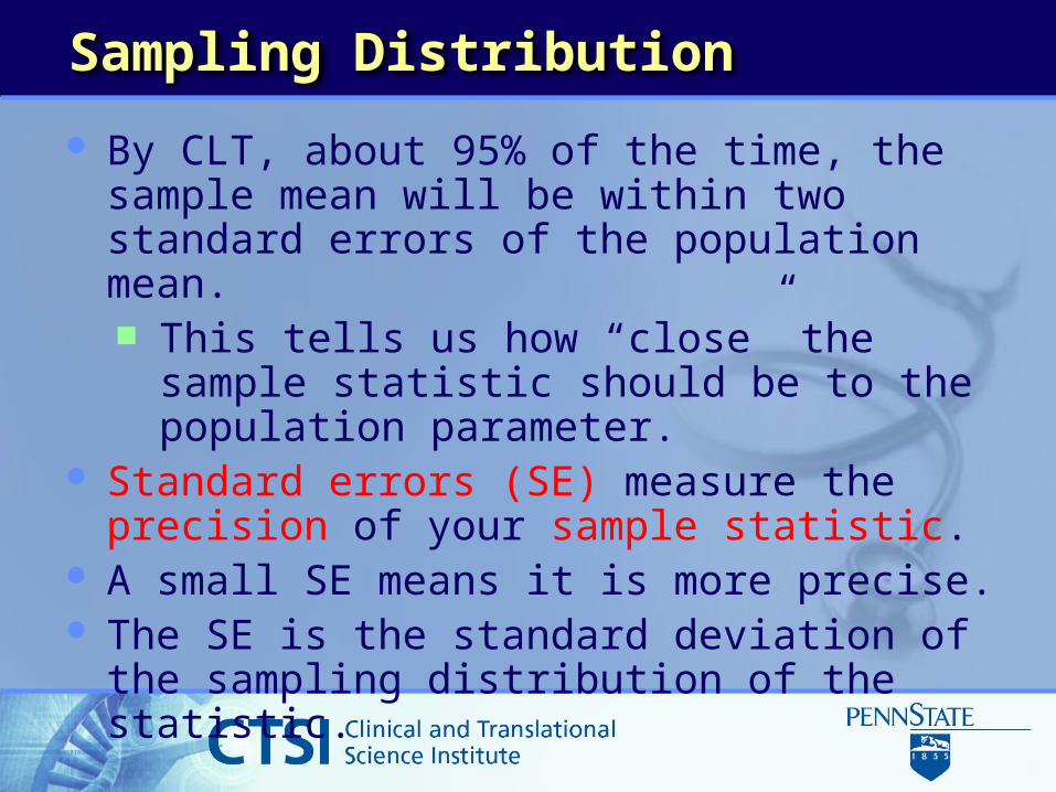
Sampling Distribution

The sampling distribution refers to the distribution of the sample statistics (e.g. sample means) over all possible samples of size n that could have been selected from the study population.

If the population data follow normal distribution N(µ, 2), then the sample means follow normal distribution N(µ, 2/n).

What if the population data do not come from normal distribution?

Central Limit Theorem (CLT)

If the sample size is large, the distribution of

sample means approximates a normal distribution. ~ N(µ, 2/n) The Central Limit Theorem works even when the

population is not normally distributed (or even not continuous).http://onlinestatbook.com/stat_sim/sampling_dist/index.html

For sample means, the standard rule is n > 60 for the Central Limit Theorem

to kick in, depending on how “abnormal” the population distribution is. 60

is a worst-case scenario.

X

Sampling Distribution

By CLT, about 95% of the time, the sample mean will be within two standard errors of the population mean. This tells us how “close” the sample statistic

should be to the population parameter. Standard errors (SE) measure the precision of

your sample statistic. A small SE means it is more precise. The SE is the standard deviation of the sampling

distribution of the statistic.

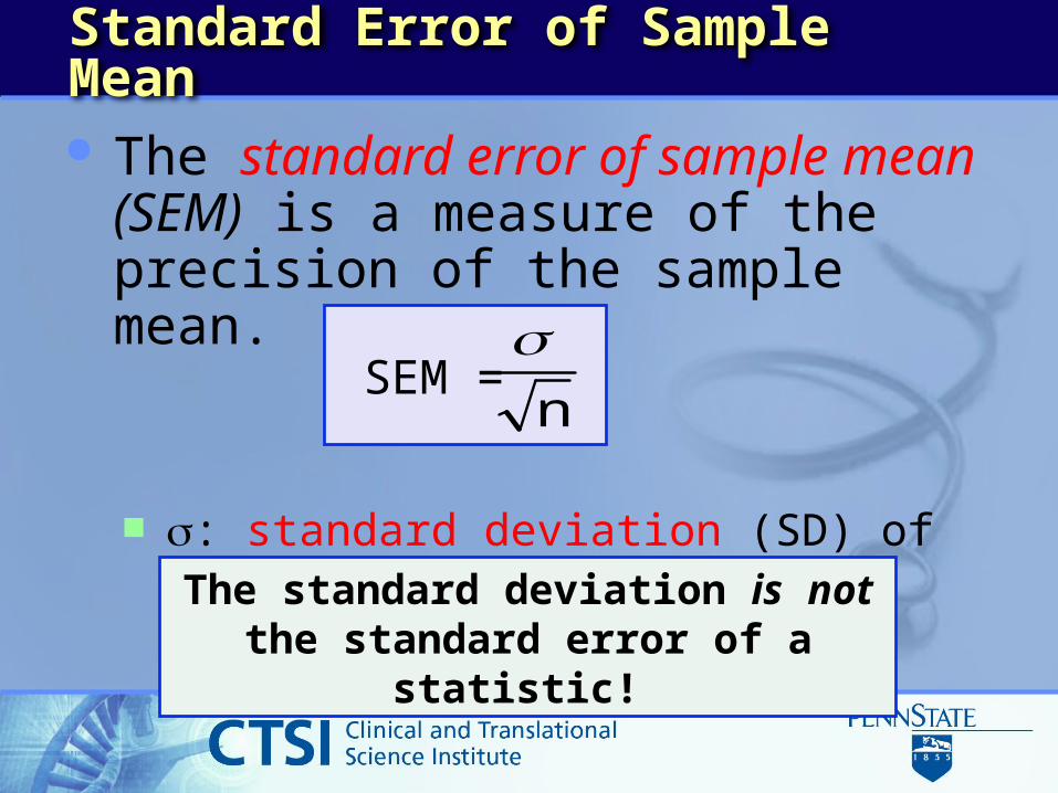
Standard Error of Sample Mean

The standard error of sample mean (SEM) is a measure of the precision of the sample mean.

: standard deviation (SD) of population distribution.

SEM =n

The standard deviation is not the standard error of a

statistic!

Example

Measure systolic blood pressure on random sample of 100 studentsSample sizen = 100Sample mean = 125 mm HgSample SD s = 14.0 mm Hg

Population SD () can be replaced by sample SD for large sample

SEM = mmHg 1.4100

14

x

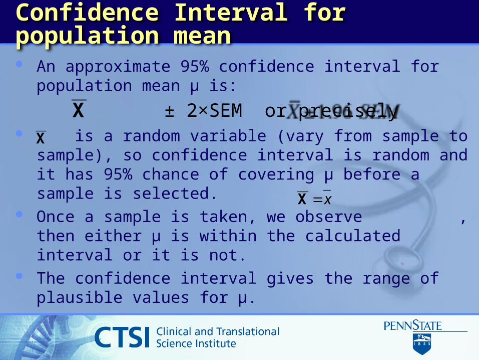
Confidence Interval for population mean

An approximate 95% confidence interval for population mean µ is:

± 2×SEM or precisely is a random variable (vary from sample to sample), so

confidence interval is random and it has 95% chance of covering µ before a sample is selected.

Once a sample is taken, we observe , then either µ is within the calculated interval or it is not.

The confidence interval gives the range of plausible values for µ.

X

xX

X