Embed Size (px)
Citation preview
Review: Stationary Time Series ModelsWhite noise process, covariance stationary process, AR(p), MA(p) and ARIMA processes, stationarity conditions, diagnostic checks.
White noise process A sequence is a white noise process if each value in the sequence has
1. zero-mean
2. constant conditional variance
3. is uncorrelated with all other realizations
Properties 1&2 : absence of serial correlation or predictabilityProperty 3 : Conditional homoscedasticity (constant conditional variance).
Covariance Stationarity (weakly stationarity)A sequence is covariance stationary if the mean, var and autocov do not grow over time, i.e. it has
1. finite mean 2. finite variance 3. finite autocovariance
Ex. autocovariance between
But white noise process does not explain macro variables characterized by persistence so we need AR and MA features.
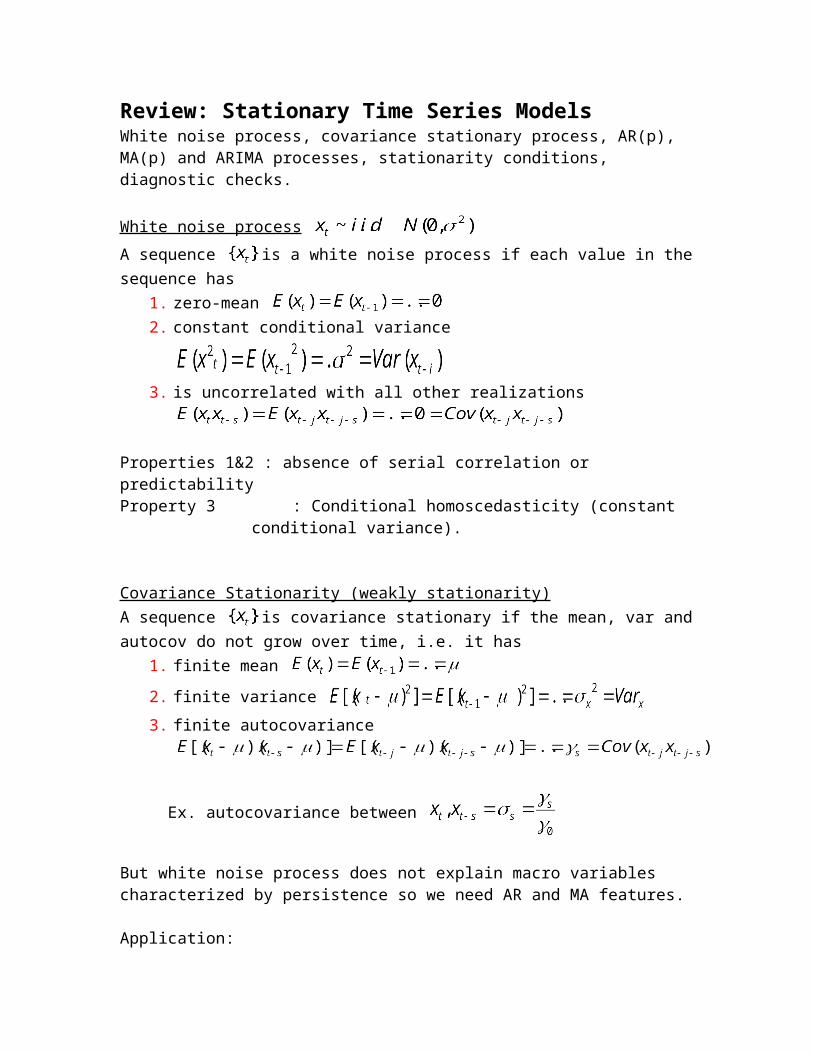
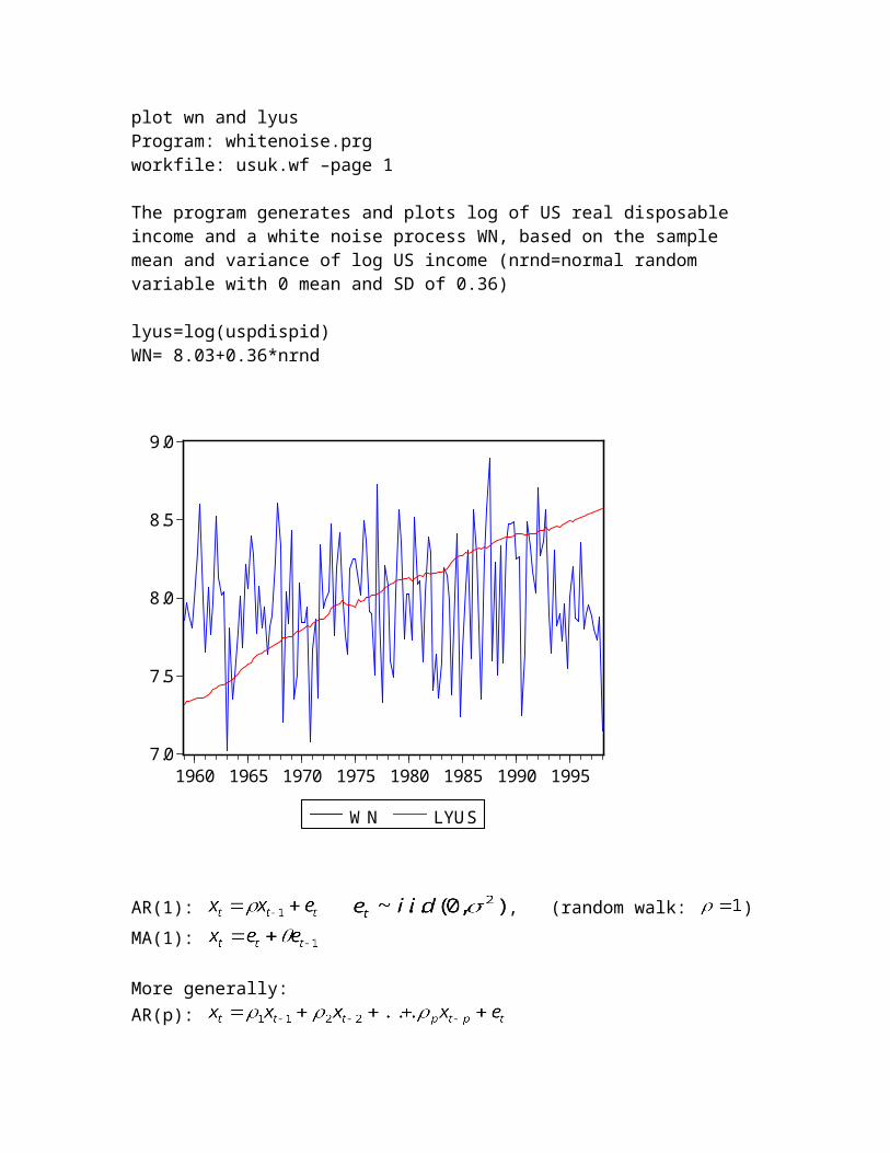
Application: plot wn and lyusProgram: whitenoise.prgworkfile: usuk.wf –page 1
The program generates and plots log of US real disposable income and a white noise process WN, based on the sample mean and variance of log US income (nrnd=normal random variable with 0 mean and SD of 0.36)
lyus=log(uspdispid)WN= 8.03+0.36*nrnd
7.0
7.5
8.0
8.5
9.0
1960 1965 1970 1975 1980 1985 1990 1995
WN LYUS
AR(1): , (random walk: )MA(1):
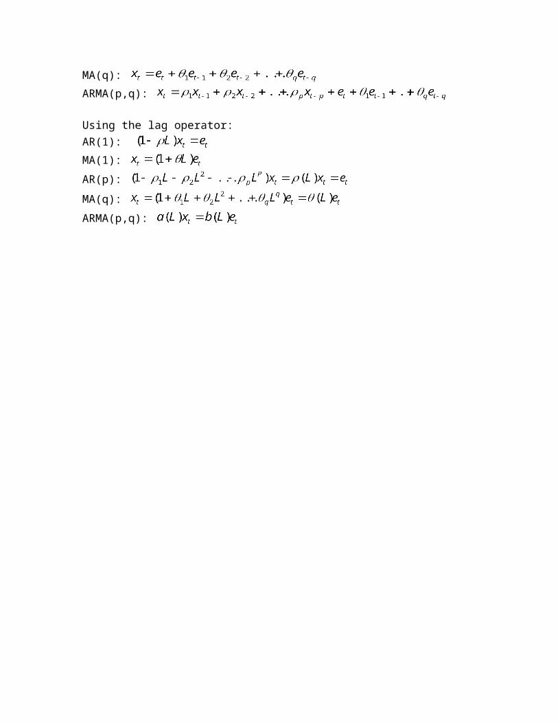
More generally:AR(p): MA(q): ARMA(p,q):
Using the lag operator:AR(1): MA(1): AR(p): MA(q): ARMA(p,q):
1. AR processStationarity Conditions for an AR(1) process
with and substituting for L:
The process is stable if for all numbers satisfying . Then we can write
If x is stable, it is covariance stationary:1. or 0 – finite
2. -- finite
3. covariances
Autocorrelations between :
Plot of over time = Autocorrelation function (ACF) or correlogram.
For stationary series, ACF should converge to 0:
if
direct convergence dampened oscillatory path around 0.
Partial Autocorrelation (PAC)Ref: Enders Ch.2
In AR(p) processes all x’s are correlated even if they don’t appear in the regression equation.Ex: AR(1)
; ;
We want to see the direct autocorrelation between and by controlling for all x’s between the two. For this, construct the demeaned series and form regressions to get the PAC from the ACs.1st PAC:
2nd PAC:
.
In general, for , sth PAC:
and .
Ex: for s=3, .
Identification for an AR(p) processPACF for s>p:
Hence AR(1):
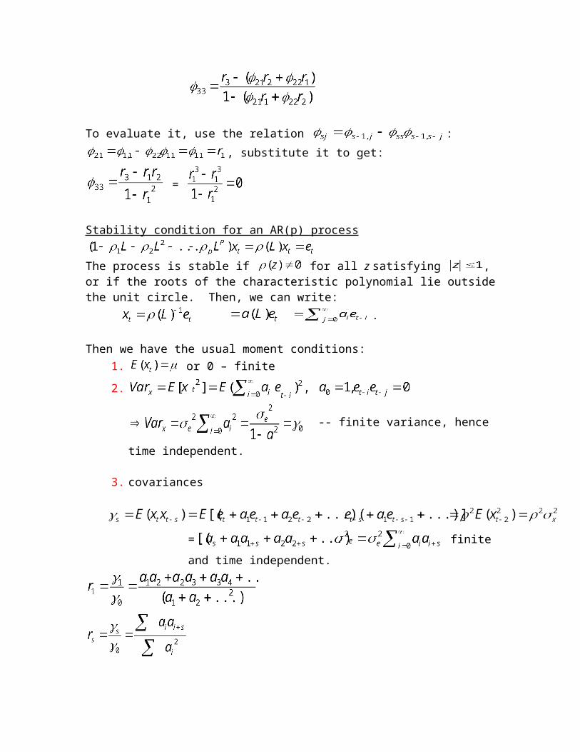
To evaluate it, use the relation :, substitute it to get:
=
Stability condition for an AR(p) process
The process is stable if for all z satisfying , or if the roots of the characteristic polynomial lie outside the unit circle. Then, we can write:
.
Then we have the usual moment conditions:1. or 0 – finite
2.
-- finite variance, hence time independent.
3. covariances
= finite and time independent.
If the process is nonstationary, what do we do?Then there is a unit root, i.e. the polynomial has a root for z=1 . We can thus factor out the operator and transform the process into a first-difference stationary series:
-- an AR(p-1) model.
If has all its roots outside the unit circle, is stationary:
If still has a unit root, we must difference it further until we obtain a stationary process:
An integrated process = a unit root process. unconditional mean is still finite but Variance is time dependent Covariance is time dependent
(more later).
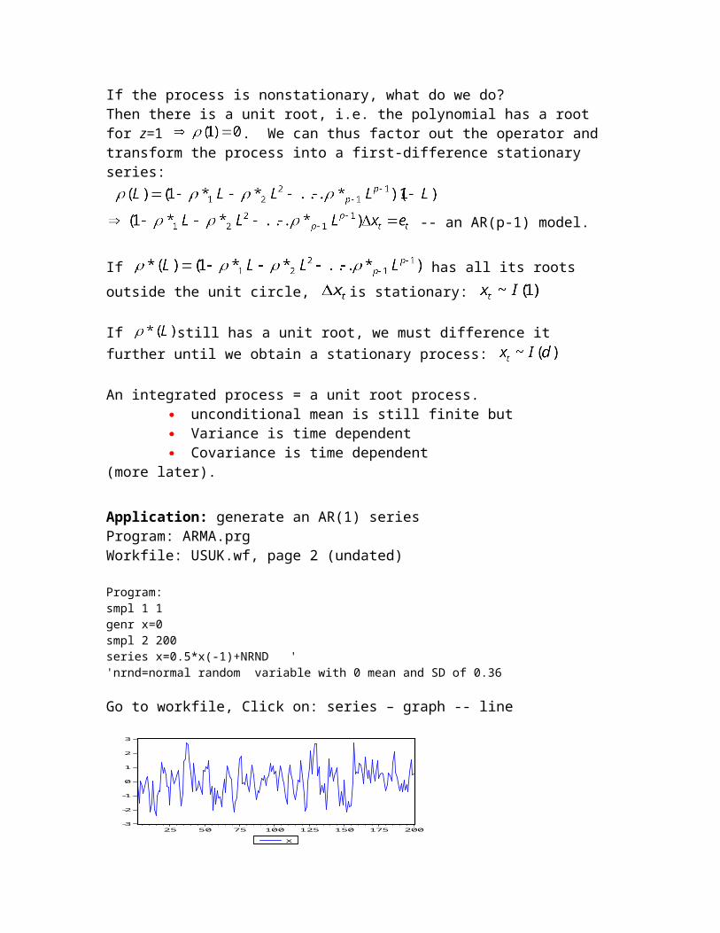
Application: generate an AR(1) seriesProgram: ARMA.prgWorkfile: USUK.wf, page 2 (undated)
Program:smpl 1 1genr x=0smpl 2 200series x=0.5*x(-1)+NRND '
'nrnd=normal random variable with 0 mean and SD of 0.36
Go to workfile, Click on: series – graph -- line
-3
-2
-1
0
1
2
3
25 50 75 100 125 150 175 200
X
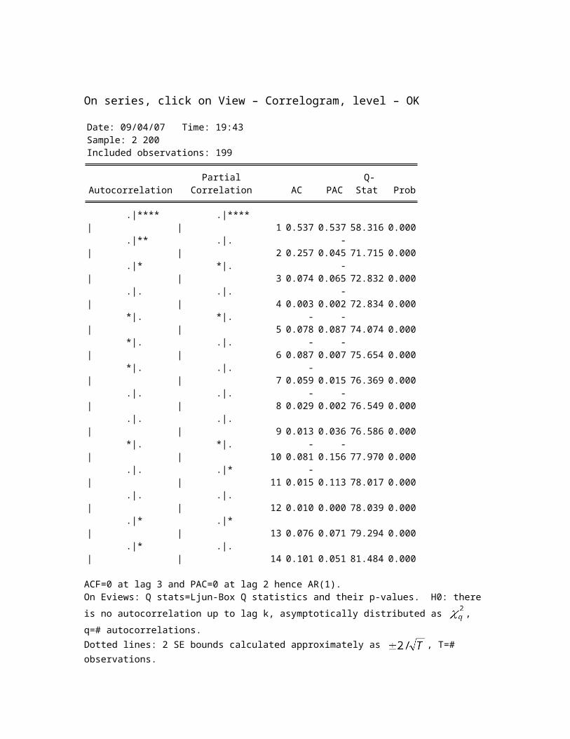
On series, click on View – Correlogram, level – OK
Date: 09/04/07 Time: 19:43Sample: 2 200Included observations: 199
Autocorrelation Partial Correlation AC PAC Q-Stat Prob
.|**** | .|**** | 1 0.537 0.537 58.316 0.000 .|** | .|. | 2 0.257 -0.045 71.715 0.000 .|* | *|. | 3 0.074 -0.065 72.832 0.000 .|. | .|. | 4 0.003 -0.002 72.834 0.000 *|. | *|. | 5 -0.078 -0.087 74.074 0.000 *|. | .|. | 6 -0.087 -0.007 75.654 0.000 *|. | .|. | 7 -0.059 0.015 76.369 0.000 .|. | .|. | 8 -0.029 -0.002 76.549 0.000 .|. | .|. | 9 0.013 0.036 76.586 0.000 *|. | *|. | 10 -0.081 -0.156 77.970 0.000 .|. | .|* | 11 -0.015 0.113 78.017 0.000 .|. | .|. | 12 0.010 0.000 78.039 0.000 .|* | .|* | 13 0.076 0.071 79.294 0.000 .|* | .|. | 14 0.101 0.051 81.484 0.000
ACF=0 at lag 3 and PAC=0 at lag 2 hence AR(1).On Eviews: Q stats=Ljun-Box Q statistics and their p-values. H0: there is no autocorrelation up to lag k, asymptotically distributed as , q=# autocorrelations.
Dotted lines: 2 SE bounds calculated approximately as , T=# observations.Here: T=199 hence SE bounds =0.14.
Program:smpl 1 1genr xa=0smpl 2 200series xa= -0.5*xa(-1)+NRND
rho=-0.5 dampened oscillatory path.
smpl 1 1genr w=0smpl 2 200series w=w(-1)+NRND
rho=1 random walk unit root.
2. MA process, e = 0 mean white noise error term.
=
If for , the process is invertible, and has an representation: =
Stability condition for MA(1) process
Invertibility requires Then the AR representation would be:
finite finite.
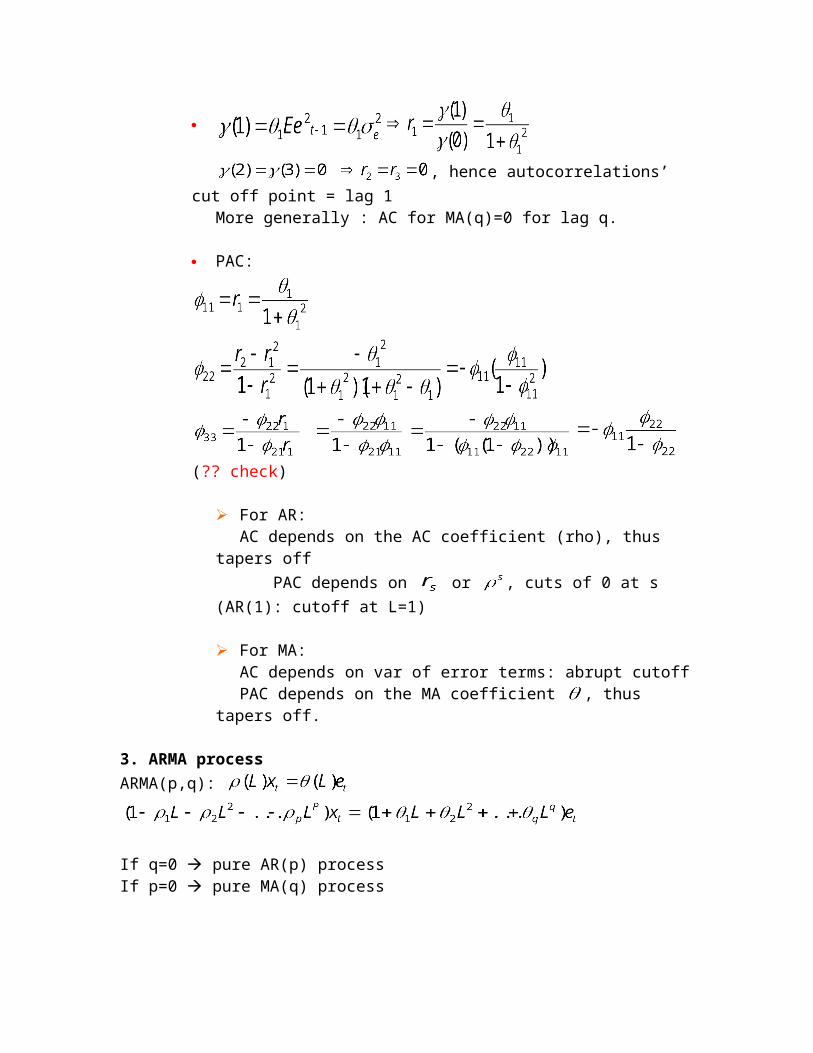
, hence autocorrelations’ cut off point = lag 1More generally : AC for MA(q)=0 for lag q.
PAC:
(??
check)
For AR: AC depends on the AC coefficient (rho), thus tapers off
PAC depends on or , cuts of 0 at s (AR(1): cutoff at L=1)
For MA:AC depends on var of error terms: abrupt cutoffPAC depends on the MA coefficient , thus tapers off.
3. ARMA processARMA(p,q):
If q=0 pure AR(p) processIf p=0 pure MA(q) process
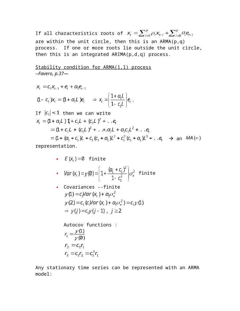
If all characteristics roots of are within the unit circle, then this is an ARMA(p,q) process. If one or more roots lie outside the unit circle, then this is an integrated ARIMA(p,d,q) process.
Stability condition for ARMA(1,1) process --Favero, p.37—
.
If then we can write
an representation.
finite
finite
Covariances --finite
Autocov functions :
Any stationary time series can be represented with an ARMA model:
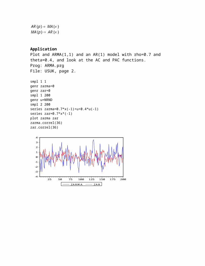
ApplicationPlot and ARMA(1,1) and an AR(1) model with rho=0.7 and theta=0.4, and look at the AC and PAC functions.Prog: ARMA.prgFile: USUK, page 2.
smpl 1 1genr zarma=0genr zar=0smpl 1 200genr u=NRNDsmpl 2 200series zarma=0.7*x(-1)+u+0.4*u(-1)series zar=0.7*x*(-1)plot zarma zarzarma.correl(36) zar.correl(36)
-4
-3
-2
-1
0
1
2
3
4
25 50 75 100 125 150 175 200
ZARMA ZAR
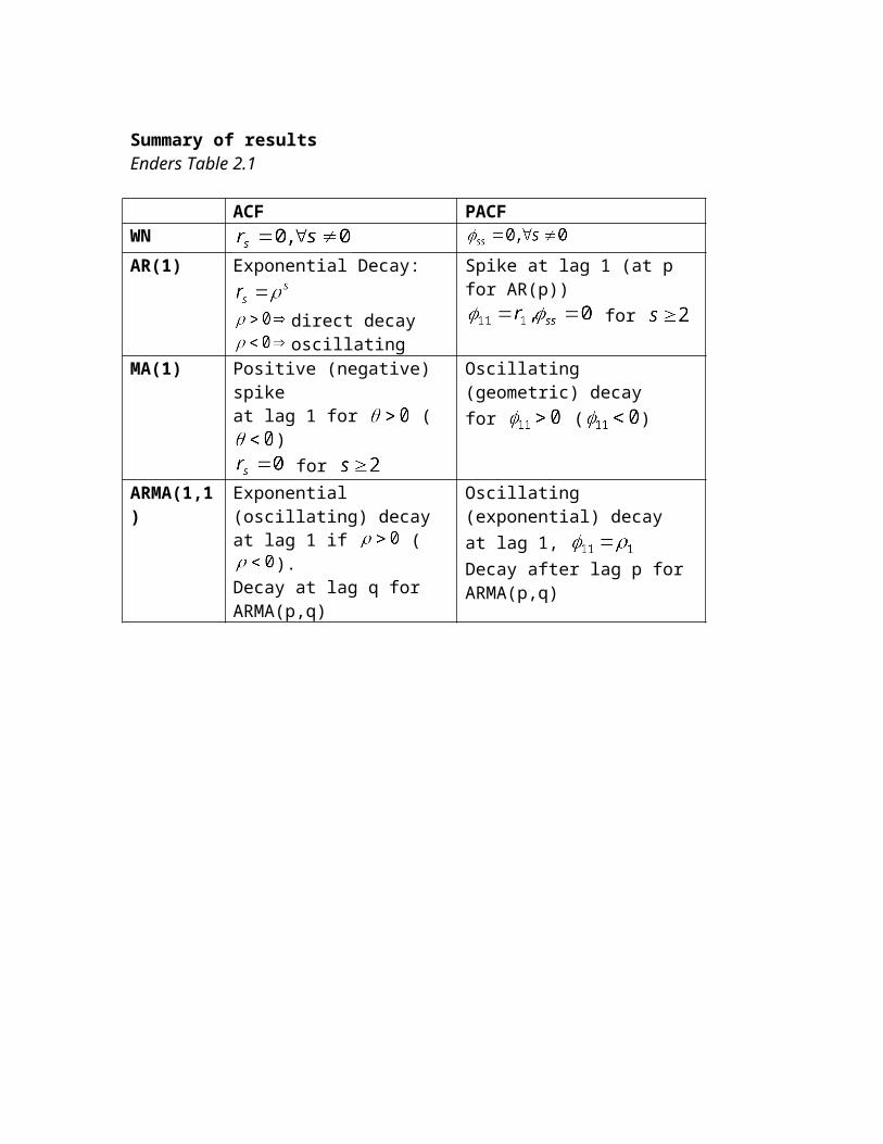
Summary of resultsEnders Table 2.1
ACF PACFWNAR(1) Exponential Decay:
direct decayoscillating
Spike at lag 1 (at p for AR(p)) for
MA(1) Positive (negative) spikeat lag 1 for ( )
for
Oscillating (geometric) decay for ( )
ARMA(1,1) Exponential (oscillating) decayat lag 1 if ( ).Decay at lag q for ARMA(p,q)
Oscillating (exponential) decayat lag 1, Decay after lag p for ARMA(p,q)
Stationary Time Series II
Model Specification and Diagnostic testsE+L&K Ch 2.5,2.6
So far we saw the theoretical properties of stationary TS. To decide about the type of model to use, we need to decide about the order of operators (# lags), the deterministic trends, etc. We therefore need to specify a model and then conduct tests on its specification, whether it represents the DGP adequately.
1. Order specification criteria:
i. The t/F-statistics approach: start from a large number of lags, and reestimate by reducing by one lag every time. Stop when the last lag is significant. Monthly data: look at the t-stats for the last lag, and F-stats for the last quarter. Then check if the error term is white noise.
ii. Information Criteria: AIC, HQ or SBC
Definition in Enders:
Akaike: AIC=T.log(SSR)+2n
Schwarz: SBC=T.log(SSR)+n.log(T) also called Schwartz and Risanen.
Hannan-Quinn:HQC=T. log(SSR)+2n.log(log(T))
T=#observations, n=#parameters estimated, including the constant term.Adding additional lags will reduce the SSR, these criteria penalize the loss of degree of freedom that comes along with additional lags.
The goal=pick the #lag that minimizes the information criteria.
Since ln(T)>2, SBS selects a more parsimonious model than AIC.For large sample, HQC and in particular SBC is better than AIC since they have better large sample properties.
o If you go along with SBC, verify that the error term is white noise. In small samples, AIC performs better.
o If you go with AIC, then verify that the t-stats are significant. This is valid whether the processes are stationary or integrated.
Note: various software and authors use modified versions of these tests. As long as you use the criteria consistently among themselves, any version will give the same results.
For ex: definition by LK:AIC=log(SSR) + 2(n/T)
SC= log(SSR) + n(logT/T)
HQ=log(SSR) + 2n.log(logT)/T)
Definition used in Eviews :AIC=-2(l/T)+(2n/T)
SC=-2(l/T)+n(logT/T)
HQ=-2(l/T)+2n.log(logT)/T
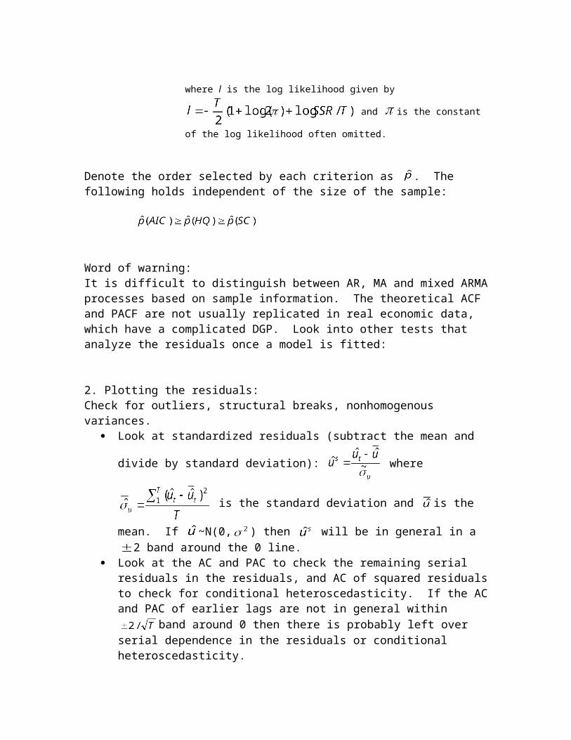
where l is the log likelihood given by
and is the constant of the log likelihood often omitted.
Denote the order selected by each criterion as . The following holds independent of the size of the sample:
Word of warning: It is difficult to distinguish between AR, MA and mixed ARMA processes based on sample information. The theoretical ACF and PACF are not usually replicated in real economic data, which have a complicated DGP. Look into other tests that analyze the residuals once a model is fitted:
2. Plotting the residuals:Check for outliers, structural breaks, nonhomogenous variances.
Look at standardized residuals (subtract the mean and divide by standard
deviation): where is the standard deviation and is
the mean. If ~N(0, ) then will be in general in a 2 band around the 0 line. Look at the AC and PAC to check the remaining serial residuals in the residuals,
and AC of squared residuals to check for conditional heteroscedasticity. If the AC and PAC of earlier lags are not in general within band around 0 then
there is probably left over serial dependence in the residuals or conditional heteroscedasticity.
3. Diagnostic tests for residuals:
i. Test of whether the kth order autocorrelation is significantly different from zero:The null hypothesis: there is no residual autocorrelation up to order s The alternative: there is at least one nonzero autocorrelation.
and k=1,..s for at least one k=1,..s.
where is the k-th autocorrelation.If the null is rejected, then at least one r is significantly different from zero. The null is rejected for large values of Q. If there are any remaining residual autocorrelation, must use a higher order of lag.
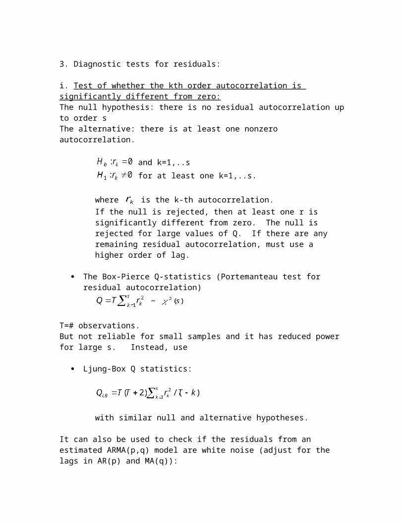
The Box-Pierce Q-statistics (Portemanteau test for residual autocorrelation) ~
T=# observations.But not reliable for small samples and it has reduced power for large s. Instead, use
Ljung-Box Q statistics:
with similar null and alternative hypotheses.
It can also be used to check if the residuals from an estimated ARMA(p,q) model are white noise (adjust for the lags in AR(p) and MA(q)):
Q~ or with a constant.
ii. Breusch-Godfrey (LM) test for autocorrelation for AR models for residuals:It considers an AR(h) model for residuals.Suppose the model you estimate is an AR(p):
You fit an auxiliary equation(*) where u is the OLS residual from the AR(p) model for y.
The LM statistics for the null: ~ , where is obtained from fitting (*).
For better small sample properties use an F version:
iii. Jarque-Bera test for nonnormalityIt tests if the standardized residuals are normally distributed, based on the third and fourth moments, by measuring the difference of the skewness and the kurtosis of the series with those from the normal distribution.
JB ~ and the null is rejected if JB is large. In this case, residuals are considered nonnormal.
Note: most of the asymptotic results are also valid for nonnormal residuals. the results may be due to nonlinearities. Then you should look into ARCH
effects or structural changes.
iv. ARCH-LM test for conditional heteroscedasticityFit an ARCH(q) model to the estimation of the residuals
and test if
. Large values of ARCH-LM show that the null is rejected and there are ARCH effects in the residuals. Then fit an ARCH or GARCH model.
v. RESETTests a model specification against alternatives (nonlinear). Ex: you are estimating a model
But the actual models is
where z can be missing variable(s) or a multiplicative relation. The test checks if powers of predicted values of y is significant. These consist of the powers and cross-product terms of the explanatory variables:
b=0 --no misspecification
The test statistics has an F(h-1,T) distribution. The null is rejected if the test statistics is too large.
vi. Stability analysisRecursive plot of residuals, of estimated coefficients; CUSUM test (cumulative sum of recursive residuals): if the plot diverges significantly from the zero line, it suggests structural instability.CUSUMSQR (square of CUSUM) in case there are several shifts in different directions.Chow test: for exogenous break points.
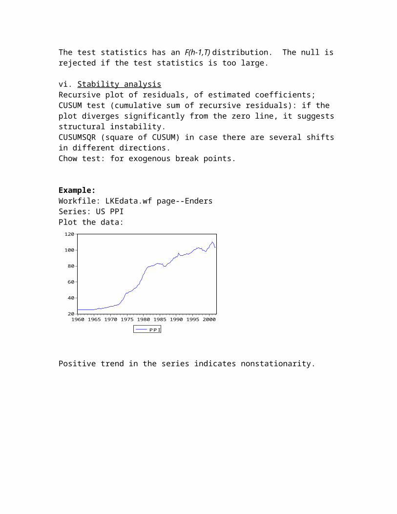
Example:Workfile: LKEdata.wf page--EndersSeries: US PPI Plot the data:
20
40
60
80
100
120
1960 1965 1970 1975 1980 1985 1990 1995 2000
PPI
Positive trend in the series indicates nonstationarity.
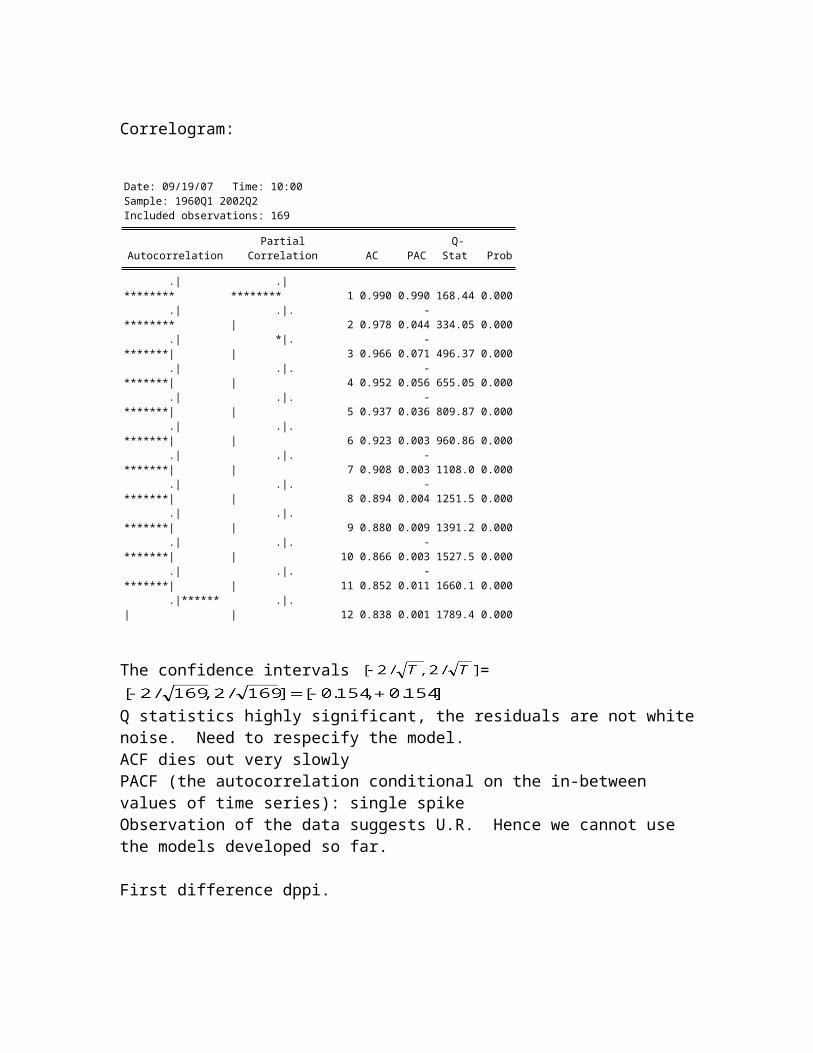
Correlogram:
Date: 09/19/07 Time: 10:00Sample: 1960Q1 2002Q2Included observations: 169
Autocorrelation Partial Correlation AC PAC Q-Stat Prob
.|******** .|******** 1 0.990 0.990 168.44 0.000 .|******** .|. | 2 0.978 -0.044 334.05 0.000 .|*******| *|. | 3 0.966 -0.071 496.37 0.000 .|*******| .|. | 4 0.952 -0.056 655.05 0.000 .|*******| .|. | 5 0.937 -0.036 809.87 0.000 .|*******| .|. | 6 0.923 0.003 960.86 0.000 .|*******| .|. | 7 0.908 -0.003 1108.0 0.000 .|*******| .|. | 8 0.894 -0.004 1251.5 0.000 .|*******| .|. | 9 0.880 0.009 1391.2 0.000 .|*******| .|. | 10 0.866 -0.003 1527.5 0.000 .|*******| .|. | 11 0.852 -0.011 1660.1 0.000 .|****** | .|. | 12 0.838 0.001 1789.4 0.000
The confidence intervals =Q statistics highly significant, the residuals are not white noise. Need to respecify the model.ACF dies out very slowlyPACF (the autocorrelation conditional on the in-between values of time series): single spikeObservation of the data suggests U.R. Hence we cannot use the models developed so far.
First difference dppi.Plot: it seems to be stationary, though the variance does not look constant, increases in the second half of the sample.
-4
-3
-2
-1
0
1
2
3
4
1960 1965 1970 1975 1980 1985 1990 1995 2000
DPPI
ACF dies out quickly after the 4th lag, and PACF has a large spike and dies out oscillating. Note the significant correlations and PAC at lag 6 and PAC at lag 8. This can be an AR(p) or an ARMA(p,q) process.
Included observations: 168
Autocorrelation Partial Correlation AC PAC Q-Stat Prob
.|**** | .|**** | 1 0.553 0.553 52.210 0.000
.|*** | .|. | 2 0.335 0.043 71.571 0.000
.|** | .|* | 3 0.319 0.170 89.229 0.000
.|** | .|. | 4 0.216 -0.042 97.389 0.000
.|* | *|. | 5 0.086 -0.081 98.682 0.000
.|* | .|* | 6 0.153 0.149 102.82 0.000
.|* | *|. | 7 0.082 -0.096 104.02 0.000
*|. | *|. | 8 -0.078 -0.149 105.10 0.000
*|. | .|. | 9 -0.080 -0.007 106.23 0.000
.|. | .|* | 10 0.023 0.121 106.33 0.000
.|. | .|. | 11 -0.008 0.004 106.34 0.000
.|. | .|. | 12 -0.006 0.007 106.35 0.000
In Eviews: run equation dppi c AR(1)(You can also run equation dppi c dppi(-1), but with the first specification Eviews estimates the model with a nonlinear algorithm, which helps controlling for nonlinearities if they exist in the DGP).
Dependent Variable: DPPIMethod: Least SquaresDate: 09/19/07 Time: 10:13Sample (adjusted): 1960Q3 2002Q1Included observations: 167 after adjustmentsConvergence achieved after 3 iterations
Variable Coefficient Std. Error t-Statistic Prob.
C 0.464364 0.133945 3.466835 0.0007AR(1) 0.554760 0.064902 8.547697 0.0000
R-squared 0.306907 Mean dependent var 0.466826Adjusted R-squared 0.302706 S.D. dependent var 0.922923S.E. of regression 0.770679 Akaike info criterion 2.328814Sum squared resid 98.00107 Schwarz criterion 2.366155Log likelihood -192.4560 F-statistic 73.06313Durbin-Watson stat 2.048637 Prob(F-statistic) 0.000000
Inverted AR Roots .55
Check the optimal lag length for an AR(p) process.Check the roots: if it is <1, stability is confirmed. View-ARMA structure-roots shows you the root(s) visually.View-ARMA structure-correlogram: allows you to compare the estimated correlations with the theoretical ones. View-ARMA structure-impulse response: shows how the DGP changes with a shock of the size of one standard deviation.View-Residual tests: to check if there is any residual autocorrelation left.
Optimal lag length:lags 1 2 3 10AIC 2.328814* 2.565575 2.575278 2.735557
SBC 2.366155* 2.603069 2.612925 2.774324
It appears that AR(1) dominates the rest in terms of the information criteria.
Roots of AR(1): 0.55<1 –stability condition satisfied, since the root is inside the unit circle.
-1.5
-1.0
-0.5
0.0
0.5
1.0
1.5
-1.5 -1.0 -0.5 0.0 0.5 1.0 1.5
AR roots
Inverse Roots of AR/MA Polynomial(s)
But serial correlation is a problem:
Breusch-Godfrey Serial Correlation LM Test:
F-statistic 3.478636 Prob. F(2,163) 0.033159Obs*R-squared 6.836216 Prob. Chi-Square(2) 0.032774
High Q stats (correlogram), and the Godfrey-Breusch test =6.84> rejects the null at the 5% confidence interval, thus there is at least one . There is serial correlation in the error terms.
Lets try ARMA(p,q):
lags 1,1 1,2 2,1AIC 2.3305* 2.3366 2.345
SBC 2.386* 2.3926 2.402
Information criteria favor an ARMA(1,1) specification although the marginal change is very small. So we should consider all options.
ARMA (1,1) -- Eviews: equation dppi c ar(1) ma(1)
Included observations: 167 after adjustments
Convergence achieved after 9 iterations
Backcast: 1960Q2
Variable Coefficient Std. Error t-Statistic Prob.
C 0.455286 0.163873 2.778280 0.0061
AR(1) 0.730798 0.100011 7.307163 0.0000
MA(1) -0.261703 0.139158 -1.880622 0.0618
R-squared 0.313995 Mean dependent var 0.466826
Adjusted R-squared 0.305629 S.D. dependent var 0.922923
S.E. of regression 0.769062 Akaike info criterion 2.330510
Sum squared resid 96.99884 Schwarz criterion 2.386522
Log likelihood -191.5976 F-statistic 37.53259
Durbin-Watson stat 1.935301 Prob(F-statistic) 0.000000
Inverted AR Roots .73
Inverted MA Roots .26
Both roots inside the unit circle. AR and MA coefficients significant.Some of the AC at larger lags are significant.LM test: =5.29 < does not reject no serial correlation in the error terms.
Notice that if you estimate an ARMA(1,2) the MA coefficient is insignificant. Together with the information criteria, we can rule out this specification. The LM test results also do not support this specification.
Variable Coefficient Std. Error t-Statistic Prob.
C 0.457550 0.176196 2.596826 0.0103
AR(1) 0.807616 0.120152 6.721624 0.0000
MA(1) -0.280755 0.148664 -1.888526 0.0607
MA(2) -0.152639 0.116160 -1.314038 0.1907
R-squared 0.322970 Mean dependent var 0.466826
Adjusted R-squared 0.310509 S.D. dependent var 0.922923
S.E. of regression 0.766355 Akaike info criterion 2.329317
Sum squared resid 95.72980 Schwarz criterion 2.404000
Log likelihood -190.4980 F-statistic 25.91910
Durbin-Watson stat 2.011448 Prob(F-statistic) 0.000000
Inverted AR Roots .81
Inverted MA Roots .56 -.27
ARMA (2,1) is better than ARMA(1,2) but does not dominate ARMA(1,1). The estimated coefficients are significant, but there is residual serial correlation.
We can perform additional tests to check the stability of the coefficient, seasonal effects, etc.
SeasonalityCyclical movements observed in daily, monthly or quarterly data. Often it is useful to remove it if it is visible in lags s, 2s, 3s, …. of the ACF and the PACF. You add an AR or MA coefficient at the appropriate lag.
Possibilities:Quarterly seasonality with MA at lag 4:
Quarterly seasonality with AR at lag 4:
Multiplicative seasonalityAccounts for interaction of the ARMA and seasonal effects.
MA term at lag 1 interacting with the seasonal MA term at lag 4:
AR term at lag 1 interacting with the seasonal AR term at lag 4:
One solution to remove strong seasonality is to transform the data by seasonal differencing. For quarterly data: If the data is not stationary, then also need to first difference it:
Eviews: Several methodologies for seasonal adjustment
Series—Proc—Seasonal AdjustmentCensus X12Census 11Moving Average MethodsTramo-Seat method
The first two options allow additive or multiplicative specifications, control for holidays, trading days, outliers.
Homework: due September 26, 2007Data: Enders Question 12.