This content has been downloaded from IOPscience. Please scroll down to see the full text.

Download details:

IP Address: 58.100.51.154

This content was downloaded on 15/03/2014 at 15:37

Please note that terms and conditions apply.

Stationary propagation of a wave segment along an inhomogeneous excitable stripe

View the table of contents for this issue, or go to the journal homepage for more

2014 New J. Phys. 16 033012

(http://iopscience.iop.org/1367-2630/16/3/033012)

Home Search Collections Journals About Contact us My IOPscience

Stationary propagation of a wave segment along aninhomogeneous excitable stripe

Xiang Gao1, Hong Zhang1, Vladimir Zykov2 and Eberhard Bodenschatz21 Zhejiang Institute of Modern Physics and Department of Physics, Zhejiang University,Hangzhou 310027, Peopleʼs Republic of China2Max Planck Institute for Dynamics and Self-Organization, D-37077 Goettingen, GermanyE-mail: vladzykov@gmail.com

Received 10 October 2013, revised 13 February 2014Accepted for publication 17 February 2014Published 13 March 2014

New Journal of Physics 16 (2014) 033012

doi:10.1088/1367-2630/16/3/033012

AbstractWe report a numerical and theoretical study of an excitation wave propagatingalong an inhomogeneous stripe of an excitable medium. The stripe inhomo-geneity is due to a jump of the propagation velocity in the direction transverse tothe wave motion. Stationary propagating wave segments of rather complicatedcurved shapes are observed. We demonstrate that the stationary segment shapestrongly depends on the initial conditions which are used to initiate the excitationwave. In a certain parameter range, the wave propagation is blocked at theinhomogeneity boundary, although the wave propagation is supported every-where within the stripe. A free-boundary approach is applied to describe thesephenomena which are important for a wide variety of applications from cardi-ology to information processing.

Keywords: excitable medium, wave segment, inhomogeneous, propagationblock

1. Introduction

Many active distributed systems in physics, biology or chemistry can be considered as excitablemedia, which are able to support an undamped propagation of excitation waves [1–4]. Forinstance, excitation waves have been observed experimentally in a wide variety of systems

New Journal of Physics 16 (2014) 0330121367-2630/14/033012+16$33.00 © 2014 IOP Publishing Ltd and Deutsche Physikalische Gesellschaft

Content from this work may be used under the terms of the Creative Commons Attribution 3.0 licence.Any further distribution of this work must maintain attribution to the author(s) and the title of the work, journal

citation and DOI.

including the oxidation reaction of CO on platinum single crystal [5], the chemicalBelousov–Zhabotinsky reaction [6], slime mold aggregation [7], electrical activity of cardiactissue [8], chicken retinas [9], and intracellular calcium waves [10]. Mathematical models ofexcitable media can usually be written in the form of essentially nonlinear reaction–diffusionsystems, which are far away from thermodynamic equilibrium.

While a study of wave dynamics in homogeneous media is a necessary starting point forclarifying the corresponding theoretical backgrounds, wave processes in inhomogeneous mediahave always been considered as a fundamental problem for many applications and attractgrowing interest nowadays. Indeed, it is extremely important to elucidate the role of aninhomogeneity as a factor which affects wave structures existing in homogeneous media oreven creates quite unusual ones [11–16]. Of course, this is very important for diverseapplications because inhomogeneity is quite natural in all real systems. For instance, incardiology the mediumʼs inhomogeneity is considered as a crucial reason for the wave breakingand the appearance of the arrhythmia [17]. On the other hand, the mediumʼs inhomogeneity canbe efficiently used to suppress life treating arrhythmia [18, 19]. Moreover, there is a tendency tocreate a mediumʼs inhomogeneity artificially, e.g. to develop structured excitable media forinformation processing [20–22].

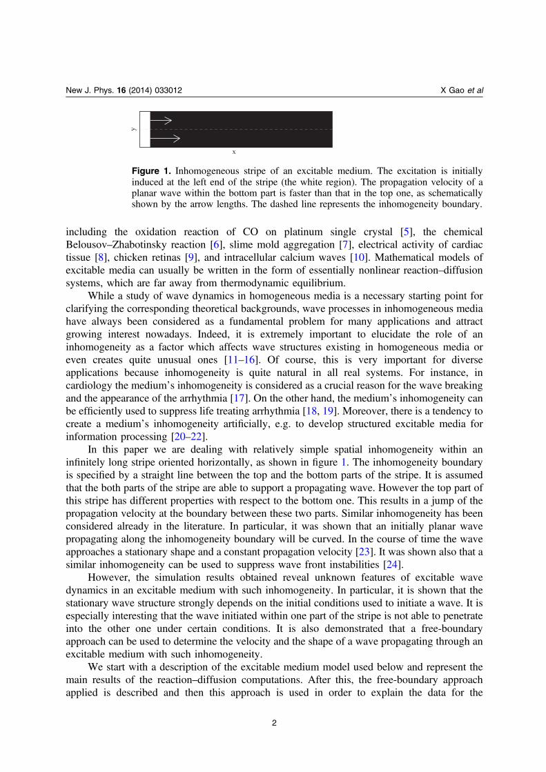
In this paper we are dealing with relatively simple spatial inhomogeneity within aninfinitely long stripe oriented horizontally, as shown in figure 1. The inhomogeneity boundaryis specified by a straight line between the top and the bottom parts of the stripe. It is assumedthat the both parts of the stripe are able to support a propagating wave. However the top part ofthis stripe has different properties with respect to the bottom one. This results in a jump of thepropagation velocity at the boundary between these two parts. Similar inhomogeneity has beenconsidered already in the literature. In particular, it was shown that an initially planar wavepropagating along the inhomogeneity boundary will be curved. In the course of time the waveapproaches a stationary shape and a constant propagation velocity [23]. It was shown also that asimilar inhomogeneity can be used to suppress wave front instabilities [24].

However, the simulation results obtained reveal unknown features of excitable wavedynamics in an excitable medium with such inhomogeneity. In particular, it is shown that thestationary wave structure strongly depends on the initial conditions used to initiate a wave. It isespecially interesting that the wave initiated within one part of the stripe is not able to penetrateinto the other one under certain conditions. It is also demonstrated that a free-boundaryapproach can be used to determine the velocity and the shape of a wave propagating through anexcitable medium with such inhomogeneity.

We start with a description of the excitable medium model used below and represent themain results of the reaction–diffusion computations. After this, the free-boundary approachapplied is described and then this approach is used in order to explain the data for the

New J. Phys. 16 (2014) 033012 X Gao et al

2

Figure 1. Inhomogeneous stripe of an excitable medium. The excitation is initiallyinduced at the left end of the stripe (the white region). The propagation velocity of aplanar wave within the bottom part is faster than that in the top one, as schematicallyshown by the arrow lengths. The dashed line represents the inhomogeneity boundary.

reaction–diffusion simulation. In the final part of the paper we discuss a wave propagation blockwhich has been observed unexpectedly in the simulations.

2. The excitable medium model

Many basic features of waves propagating in excitable media can be analyzed by means of ageneric two-component reaction–diffusion model of the form [25]

ε∂∂

= + ∂∂

=u

tD u F u v

v

tG u v( , ), ( , ), (1)2

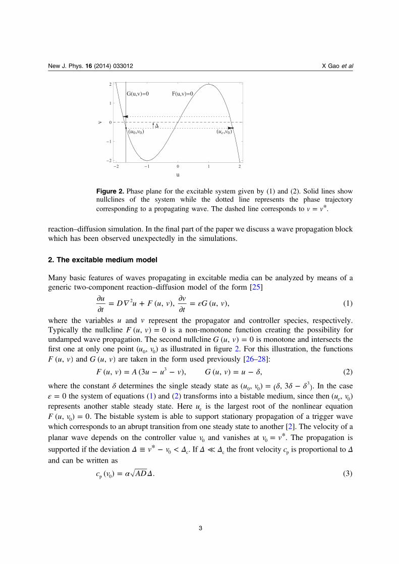
where the variables u and v represent the propagator and controller species, respectively.Typically the nullcline =F u v( , ) 0 is a non-monotone function creating the possibility forundamped wave propagation. The second nullcline =G u v( , ) 0 is monotone and intersects thefirst one at only one point (u v,0 0) as illustrated in figure 2. For this illustration, the functionsF u v( , ) and G u v( , ) are taken in the form used previously [26–28]:

δ= − − = −F u v A u u v G u v u( , ) (3 ), ( , ) , (2)3

where the constant δ determines the single steady state as δ δ δ= −u v( , ) ( , 3 )0 03 . In the case

ε = 0 the system of equations (1) and (2) transforms into a bistable medium, since then u v( , )e 0

represents another stable steady state. Here ue is the largest root of the nonlinear equation=F u v( , ) 00 . The bistable system is able to support stationary propagation of a trigger wave

which corresponds to an abrupt transition from one steady state to another [2]. The velocity of aplanar wave depends on the controller value v0 and vanishes at = *v v0 . The propagation is

supported if the deviation Δ Δ≡ − <*v v0 c. If Δ Δ≪ c the front velocity cp is proportional to Δand can be written as

α Δ=c v AD( ) . (3)p 0

New J. Phys. 16 (2014) 033012 X Gao et al

3

Figure 2. Phase plane for the excitable system given by (1) and (2). Solid lines shownullclines of the system while the dotted line represents the phase trajectorycorresponding to a propagating wave. The dashed line corresponds to = *v v .

The constants α, *v and Δc are determined by the function F u v( , ). In particular, for the

function defined in equation (2), they can be determined analytically as α = 1/ 2 , =*v 0 andΔ = 2c .

If ε< ≪0 1, there is a single steady state u v( , )0 0 of the system (1) and (2). Asuprathreshold perturbation induces propagation of a wave including an abrupt transition fromu v( , )0 0 to practically u v( , )e 0 (wave front), slow motion along the right branch of the u-nullcline(wave plateau), and an abrupt transition to the left branch (wave back) as illustrated in figure 2.During the recovery process following the wave back the system returns to the steady state. Inthe simplest case of a homogeneous excitable stripe, such a wave exhibiting stationarypropagation along the stripe has a planar front and a planar back, which have no commonpoints.

3. Reaction–diffusion simulation results

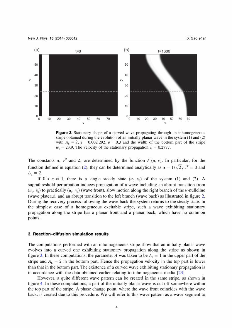
The computations performed with an inhomogeneous stripe show that an initially planar waveevolves into a curved one exhibiting stationary propagation along the stripe as shown infigure 3. In these computations, the parameter A was taken to be =A 1l in the upper part of thestripe and =A 2h in the bottom part. Hence the propagation velocity in the top part is lowerthan that in the bottom part. The existence of a curved wave exhibiting stationary propagation isin accordance with the data obtained earlier relating to inhomogeneous media [23].

However, a quite different wave pattern can be created in the same stripe, as shown infigure 4. In these computations, a part of the initially planar wave is cut off somewhere withinthe top part of the stripe. A phase change point, where the wave front coincides with the waveback, is created due to this procedure. We will refer to this wave pattern as a wave segment to

New J. Phys. 16 (2014) 033012 X Gao et al

4

50

40

30

20

10

0

y

x

50

40

30

20

10

0y

0 10 20 30 40 50 60 70x

0 10 20 30 40 50 60 70

t=0 t=1600(a) (b)

Figure 3. Stationary shape of a curved wave propagating through an inhomogeneousstripe obtained during the evolution of an initially planar wave in the system (1) and (2)with =A 2h , ε = 0.002 292, δ = 0.3 and the width of the bottom part of the stripe

=w 23.9b . The velocity of the stationary propagation =c 0.2777t .

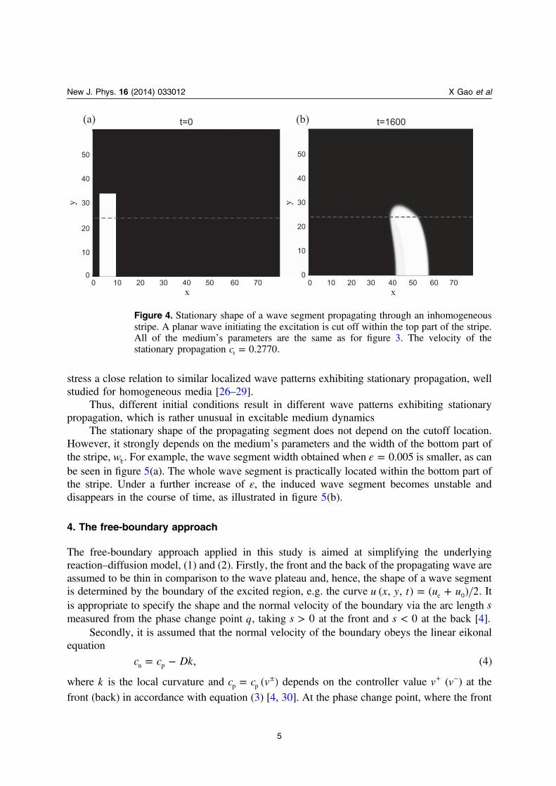
stress a close relation to similar localized wave patterns exhibiting stationary propagation, wellstudied for homogeneous media [26–29].

Thus, different initial conditions result in different wave patterns exhibiting stationarypropagation, which is rather unusual in excitable medium dynamics

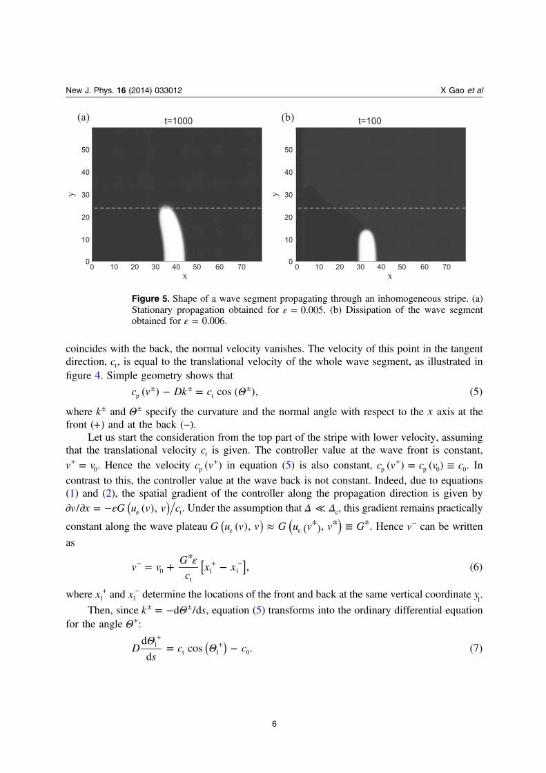
The stationary shape of the propagating segment does not depend on the cutoff location.However, it strongly depends on the mediumʼs parameters and the width of the bottom part ofthe stripe, wb. For example, the wave segment width obtained when ε = 0.005 is smaller, as canbe seen in figure 5(a). The whole wave segment is practically located within the bottom part ofthe stripe. Under a further increase of ε, the induced wave segment becomes unstable anddisappears in the course of time, as illustrated in figure 5(b).

4. The free-boundary approach

The free-boundary approach applied in this study is aimed at simplifying the underlyingreaction–diffusion model, (1) and (2). Firstly, the front and the back of the propagating wave areassumed to be thin in comparison to the wave plateau and, hence, the shape of a wave segmentis determined by the boundary of the excited region, e.g. the curve = +u x y t u u( , , ) ( ) 2e 0 . Itis appropriate to specify the shape and the normal velocity of the boundary via the arc length smeasured from the phase change point q, taking >s 0 at the front and <s 0 at the back [4].

Secondly, it is assumed that the normal velocity of the boundary obeys the linear eikonalequation

= −c c Dk, (4)n p

where k is the local curvature and = ±c c v( )p p depends on the controller value +v ( −v ) at the

front (back) in accordance with equation (3) [4, 30]. At the phase change point, where the front

New J. Phys. 16 (2014) 033012 X Gao et al

5

50

40

30

20

10

0

y

50

40

30

20

10

0y

0 10 20 30 40 50 60 70x

0 10 20 30 40 50 60 70x

t=0 t=1600(a) (b)

Figure 4. Stationary shape of a wave segment propagating through an inhomogeneousstripe. A planar wave initiating the excitation is cut off within the top part of the stripe.All of the mediumʼs parameters are the same as for figure 3. The velocity of thestationary propagation =c 0.2770t .

coincides with the back, the normal velocity vanishes. The velocity of this point in the tangentdirection, ct, is equal to the translational velocity of the whole wave segment, as illustrated infigure 4. Simple geometry shows that

Θ− =± ± ±c v Dk c( ) cos ( ), (5)p t

where ±k and Θ± specify the curvature and the normal angle with respect to the x axis at thefront (+) and at the back (−).

Let us start the consideration from the top part of the stripe with lower velocity, assumingthat the translational velocity ct is given. The controller value at the wave front is constant,

=+v v0. Hence the velocity +c v( )p in equation (5) is also constant, = ≡+c v c v c( ) ( )p p 0 0. In

contrast to this, the controller value at the wave back is not constant. Indeed, due to equations(1) and (2), the spatial gradient of the controller along the propagation direction is given by

ε∂ ∂ = − ( )v x G u v v c/ ( ),e t. Under the assumption that Δ Δ≪ c, this gradient remains practically

constant along the wave plateau ≈ ≡* * *( )( )G u v v G u v v G( ), ( ),e e . Hence −v can be written

as

ε= + −*− + −[ ]v v

G

cx x , (6)0

tl l

where +xl and −xl determine the locations of the front and back at the same vertical coordinate yl.

Then, since Θ= −± ±k sd /d , equation (5) transforms into the ordinary differential equationfor the angle Θ+:

ΘΘ= −

++( )D

sc c

d

dcos . (7)l

t l 0

New J. Phys. 16 (2014) 033012 X Gao et al

6

50

40

30

20

10

0

y

x

50

40

30

20

10

0y

0 10 20 30 40 50 60 70x

0 10 20 30 40 50 60 70

t=1000 t=100(a) (b)

Figure 5. Shape of a wave segment propagating through an inhomogeneous stripe. (a)Stationary propagation obtained for ε = 0.005. (b) Dissipation of the wave segmentobtained for ε = 0.006.

A similar transformation taking into account equation (6) yields the equation for the angle Θ −l :

Θ εαΘ=

−− +

*− + −−( )

( )Ds

G D x x

cc c

d

dcos . (8)l l l

t0 t l

Equations (7) and (8) supplemented by the obvious relationships Θ= −± ±( )y sd d cosl l and

Θ=± ±( )x sd d sinl l specify the shape of the traveling wave segment within the top part of thestripe with lower propagation velocity. The integration of the system has to be started with thefollowing initial conditions: Θ Θ π= =+ −(0) (0) /2l l , = =+ −x x x(0) (0)l l 0 and

= =+ −y y y(0) (0)l l 0

. Here x0 and y0can be chosen arbitrarily, e.g. = =x y 00 0

.To analyze possible solutions of equations (7) and (8), it is appropriate to use the value c0

in order to rescale velocities, e.g. =C c ct t 0, and space variables, e.g. =S c s D0 , =X c x D0 and=Y c y D0 , which yields for the angle Θ +

l

ΘΘ= −

++( )

SC

d

dcos 1, (9)l

t l

and for the angle Θ −l

ΘΘ=

−− +

− + −−( )

( )S

B X X

CC

d

d1 cos , (10)l l l

tt l

where

εα Δ

=*

BG

. (11)2 3

After this rescaling, one can conclude that since the initial conditions for this system are welldetermined, the solution depends on the single dimensionless parameter B. Note that for thegiven model (1) and (2) with fixed Δ = 0.3, the parameter B is simply proportional to theparameter ε.

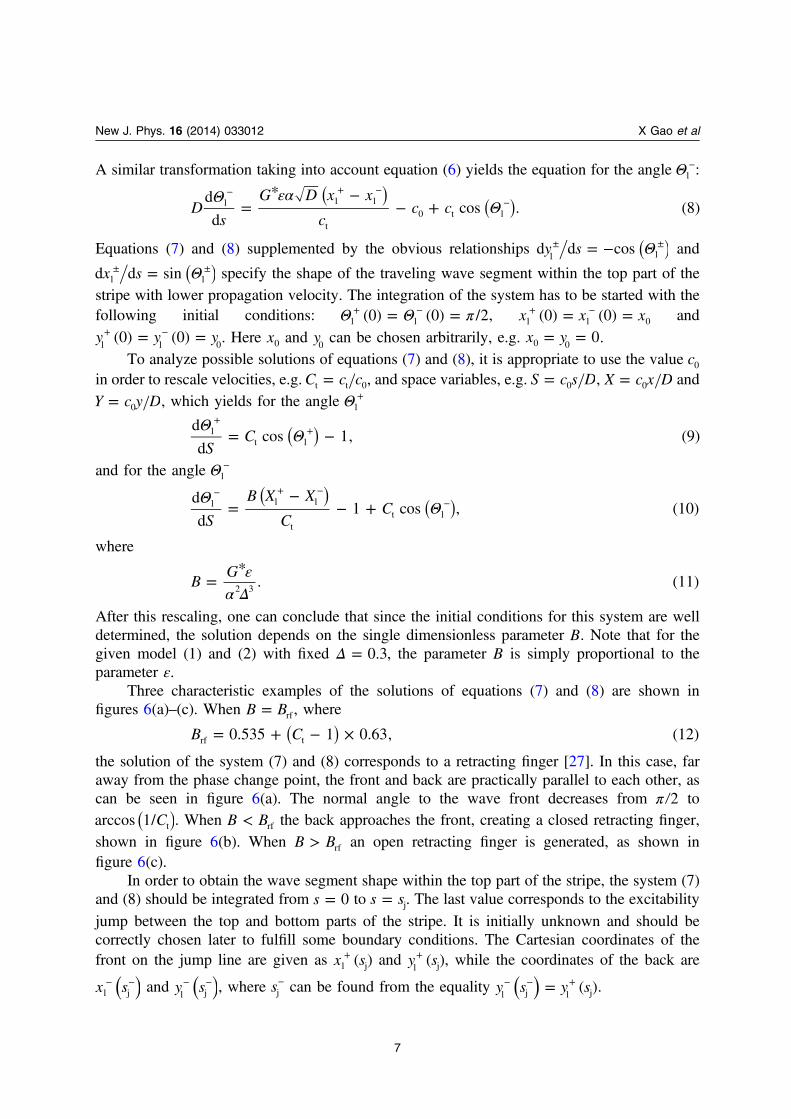
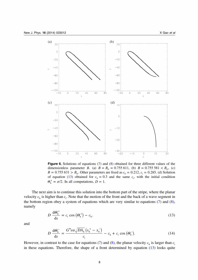
Three characteristic examples of the solutions of equations (7) and (8) are shown infigures 6(a)–(c). When =B Brf, where

= + − ×( )B C0.535 1 0.63, (12)rf t

the solution of the system (7) and (8) corresponds to a retracting finger [27]. In this case, faraway from the phase change point, the front and back are practically parallel to each other, ascan be seen in figure 6(a). The normal angle to the wave front decreases from π 2 to

( )Carccos 1/ t . When <B Brf the back approaches the front, creating a closed retracting finger,shown in figure 6(b). When >B Brf an open retracting finger is generated, as shown infigure 6(c).

In order to obtain the wave segment shape within the top part of the stripe, the system (7)and (8) should be integrated from =s 0 to =s sj. The last value corresponds to the excitability

jump between the top and bottom parts of the stripe. It is initially unknown and should becorrectly chosen later to fulfill some boundary conditions. The Cartesian coordinates of thefront on the jump line are given as +x s( )l j and +y s( )

l j , while the coordinates of the back are− −( )x sl j and − −( )y s

l j , where −sj can be found from the equality =− − +( )y s y s( )l j l j .

New J. Phys. 16 (2014) 033012 X Gao et al

7

The next aim is to continue this solution into the bottom part of the stripe, where the planarvelocity ch is higher than ct. Note that the motion of the front and the back of a wave segment inthe bottom region obey a system of equations which are very similar to equations (7) and (8),namely

ΘΘ= −

++( )D

sc c

d

dcos . (13)h

t h h

and

Θ εαΘ=

−− +

*− + −−( )

( )Ds

G DA x x

cc c

d

dcos . (14)h h h h

th t h

However, in contrast to the case for equations (7) and (8), the planar velocity ch is larger than ct

in these equations. Therefore, the shape of a front determined by equation (13) looks quite

New J. Phys. 16 (2014) 033012 X Gao et al

8

Figure 6. Solutions of equations (7) and (8) obtained for three different values of thedimensionless parameter B. (a) = =B B 0.755 611rf , (b) = <B B0.755 581 rf, (c)

= >B B0.755 631 rf. Other parameters are fixed as =c 0.2120 , =c 0.285t . (d) Solutionof equation (13) obtained for =c 0.3h and the same ct, with the initial conditionΘ π=+ /2h . In all computations, =D 1.

different in comparison to the solution of equation (7), as can be seen in figure 6(d). This shapeis identical to one found earlier for stabilized wave segments [28]. Note that the normal angle inthis case reduces from π /2 to zero. This range is broader than in the case of a retracting finger.Therefore, for any given sj, it is possible to smoothly continue a solution previously found

within the top part of the stripe as Θ Θ=+ +s s( ) ( )h j l j . It is important to stress that the Cartesian

coordinates should also satisfy smoothness conditions like =+ +x s x s( ) ( )h j l j and =+ +y s y s( ) ( )h j l j .

This solution should be continued to a point =s sb, where Θ =+ s( ) 0h b , as shown infigure 6(d). Such a point always exists, since it corresponds to a symmetry axis of a stabilizedwave segment in a homogeneous medium. In the problem under consideration, this angle valueΘ =+ s( ) 0h b corresponds to the no-flux boundary conditions at the stripe bottom.

Note that the wave back should be orthogonal to the no-flux boundary at the bottom, aswell. The solution of equation (14) is completely determined by the initial condition

Θ Θ=− − − −( ) ( )s sh j l j and the shape of the wave front obtained for an arbitrarily chosen sj. The

corresponding computations show that if sj is too small, Θ π<− −( )sh b ; and if sj is too large,

Θ π>− −( )sh b . By the trial and error method, a corrected value of sj should be determined.

Thus, there is an opportunity to obtain a solution of the above formulated free-boundaryproblem corresponding to boundary conditions for the underlying reaction–diffusion system (1)and (2) by varying the single parameter sj. An example of such a solution is shown in figure 7.

Here the planar velocity in the top part is fixed to =c 0.2120 , which corresponds to Δ = 0.3 inthe system (1) and (2) due to equation (3). In the bottom part the planar velocity is =c 0.3h ,which corresponds to =A 2h . The dimensionless parameter =B 0.756 086, which correspondsto ε = 0.002 992 due to equation (11). The translational velocity of the wave segments as awhole is =c 0.285t . The solution of the free-boundary problem completely determines the wave

New J. Phys. 16 (2014) 033012 X Gao et al

9

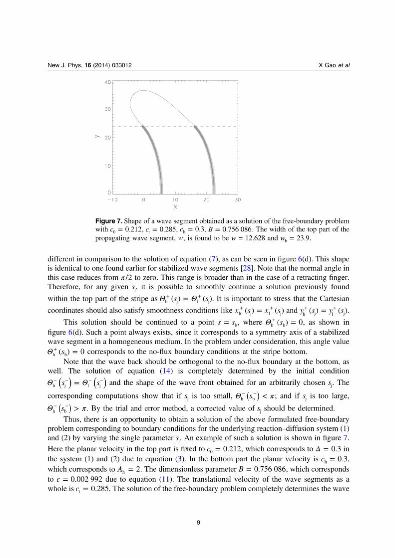
Figure 7. Shape of a wave segment obtained as a solution of the free-boundary problemwith =c 0.2120 , =c 0.285t , =c 0.3h , =B 0.756 086. The width of the top part of thepropagating wave segment, w, is found to be w = 12.628 and =w 23.9b .

segment shape. The width of the segment in the top part is determined as = −w y y s(0) ( )b .The width of the bottom part of the stripe is specified as = −w y s y s( ) ( )b j b .

5. The existence of a solution

The solution of the free-boundary problem presented in figure 7 is obtained for >B Brf, in thecase of the open retracting finger shown in figure 6(c). The parameter B can be continuouslydecreased by decreasing of ε without any significant effect on the propagation velocity. As aresult, the width of the segment in the top part of the stripe is monotonically increasing.Moreover, the width diverges when →B Brf. In this limit, the part of the wave segment withinthe top part of the stripe approaches a retracting finger, which by definition has an infinitelylarge width [27]. This means that a propagating wave segment can exist in this limiting caseonly within an infinitely broad stripe. If the stripe has a finite width and is restricted by a no-fluxboundary, a solution in the form of a wave segment does not exist. Only a curved wave similarto the one shown in figure 3 can exist in this case.

An example of a relationship ε=w w ( ) is shown in figure 8 by the thick solid line. Thewidth diverges at some ε corresponding to Brf .

The results of the corresponding reaction–diffusion computations are shown by the dashedline. It is indicated by the data obtained that the segment width also diverges at some B. Allattempts to initiate a propagating wave segment in the reaction–diffusion computations for

<B Brf lead to the creation of a curved wave.In the framework of the free-boundary approach, it is also impossible to obtain a physically

acceptable solution for <B Brf. In this case, the solution in the top part has the form of a closedretracting finger, shown in figure 6(b). While the front solution can be continued into the bottompart to a point where Θ =+ s( ) 0h b , it is impossible to reach the condition Θ π=− −( )sh b for theback solution for any sj.

Note that the accuracy of the theoretical predictions can be improved. The data shown in

figure 8 by the thick solid line are based on the analytically obtained value α = 1/ 2 under theassumption that ε ≪ 1 and Δ ≪ 1. However, this coefficient can be obtained from direct

reaction–diffusion computations, giving α = 0.943/ 2 . This small correction of the coefficientα considerably increases the prediction accuracy, as is shown by the dotted line in figure 8.

There is another restriction for the existence of a propagating wave segment, which has tobe taken into account. This restriction becomes visible in the framework of the free-boundaryapproach. Let us assume that all parameters are fixed (e.g. as in figure 7) except the translationalvelocity ct, which is continuously decreasing. Two examples of such computations are shown infigure 9. It is clear that the slower translation velocity corresponds to the larger front curvaturenear the bottom boundary of the stripe. Consequently the width of the bottom part of the stripe,wb, corresponding to this velocity becomes smaller. Simultaneously, the width of the wavesegments within the top part of the stripe, w, also becomes smaller. Figure 9(b) illustrates thelimiting case where w vanishes at =c ct tm. There is no solution of the free-boundary approachfor <c ct tm.

It is important to stress that the shape of the wave segment within the bottom part of thestripe obtained for =c ct tm should be identical to a stabilized wave segment shape observed

New J. Phys. 16 (2014) 033012 X Gao et al

10

earlier in a homogeneous medium [29]. In the last case, the dimensionless wave segment widthis completely determined by the dimensionless parameter B. Hence this parameter specified forthe bottom part of the stripe as

εα Δ

=*

BG

A(15)b

h2 3

can be used to predict the minimal width of the bottom part of the stripe. In accordance withequation (19) in [29], the translational velocity reads

= + − ⎜ ⎟⎛⎝

⎞⎠c c B

B(1 0.535)

0.535, (16)

n

t h bb

where =n 2.502. The corresponding value is depicted by the left dotted line in figure 10.

New J. Phys. 16 (2014) 033012 X Gao et al

11

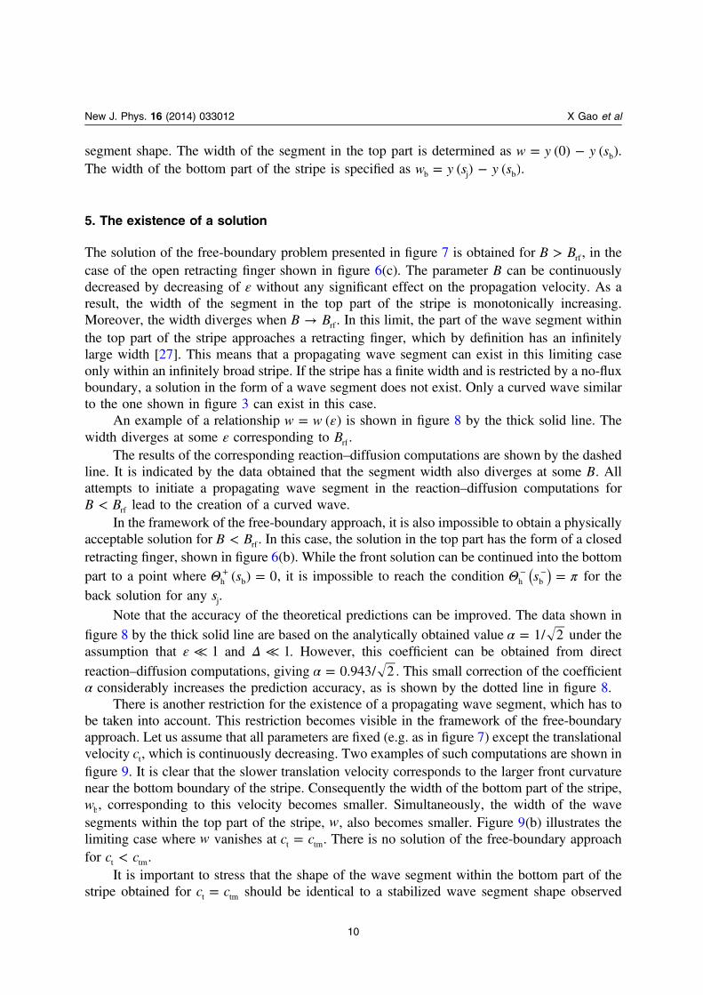
Figure 8. Width of the top part of the propagating wave segment, w, versus theparameter ε obtained for =c 0.2120 , =c 0.285t , =c 0.3h and Δ = 0.3 (thick solid line)and the results of reaction–diffusion computations (the dashed line). The dotted linecorresponds to the free-boundary computations with α = 0.943/ 2 .

Figure 9. Shape of a wave segment obtained as a solution of the free-boundary problemwith =c 0.2120 , =c 0.3h , =B 0.756 086. (a) =c 0.275t , (b) = =c c 0.2281t tm . Thereis no solution for <c ct tm.

Note that a curved wave solution exists in an inhomogeneous stripe even if the part withhigh propagation velocity is very thin [23]. Thus, starting from a planar wave, a propagatingwave solution can exist in the form of a curved wave, but a wave solution can disappear if alocalized wave segment has been used as an initial condition.

Thus, if all parameters of the free-boundary system are fixed, a wave segment solutionexists within a restricted interval of the translational velocity ct as shown in figure 10. At the leftedge of this parameter range, the width of the wave segment within the top part of the stripe, w,vanishes and the solution corresponds to the one shown in figure 9(b). At the right edge thewidth of the wave segment within the top part of the stripe, w, diverges.

It is important that a well determined range of the width Wb corresponds to this interval ofCt in which a wave segment solution can exist, as illustrated by figure 10. Note that thetranslation velocity Ct is used as a control parameter in the framework of the free-boundaryapproach. In contrast to this, in reaction–diffusion computations or real experiments the widthof the bottom part of the stripe has to be considered as the control parameter which determinesthe translational velocity Ct. Thus, a wave segment solution exists in a restricted range of thebottom part width.

6. Two asymptotes for translational velocity

It follows from the above consideration that for given parameters c0, ch and ct, which satisfy thecondition < <c c c0 t h, there is a physically acceptable front solution. This solution correspondsto a well determined width, wb, of the bottom part of the stripe. Thus, independently of B, thereis a relationship between the three given velocities and the width wb.

On the other hand, there is a curved wave solution shown in figure 3. As was mentioned in[23] in the case of an infinite width of the top part of the stripe, the normal angle near the

New J. Phys. 16 (2014) 033012 X Gao et al

12

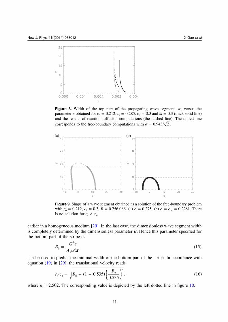
Figure 10. Dimensionless width of the bottom part of the stripe =W w c Db b h versus thedimensionless translational velocity =C c ct t h obtained from the free-boundarycomputations (the thick solid line and symbols ‘+’). The free-boundary system has asolution only within a parameter region restricted by two dotted lines. An analyticalestimate due to equation (19) for a curved wave solution is shown by the thin solid line.The width of a wave segment propagating through a homogeneous medium is shown bythe dashed line. All computations correspond to =c c 2h 0 .

excitability jump approaches

Θ =+ ( )s c c( ) arccos . (17)l j 0 t

Moreover, a solution of equation (13) can be expressed analytically [23] as

Θ= − +

−

+

−

Θ+ ++

y

D c

c

c c c

c c

c c

2arctan

( ) tan. (18)h h

t

h

t h2

t2

h t 2

h2

t2

h

Since the width of the bottom part can be expressed as Θ= −+ + +( )w y s y( ) (0)b h l j h, substitution

of equation (17) into equation (18) gives the width of the bottom part as

= − +−

+

−

( )w

D

c c

c

c

c c c

c c

c c

arccos 2arctan

( ) tan. (19)

c c

b 0 t

t

h

t h2

t2

h tarccos ( )

2

h2

t2

0 t

An example of this relationship is shown in figure 10 by the thin line. Here the

dimensionless width =W w c Db b h is presented as a function of c ct h for =c c 2h 0 . Note thatthe solution in the form of a wave segment approaches this relationship in the limiting casewhen the width w diverges. For a given value of the parameter B, this happens when thetranslational velocity satisfies equation (12) (depicted by the right dotted line in figure 10).

It is necessary to stress that, at the left edge of the existence region, the free-boundarysolution approaches a wave segment propagating within the bottom part of the stripe, as shownin figure 9(b). In order to get a relationship between the translational velocity and the width ofsuch a segment, it is enough to repeat the above consideration keeping Θ π=+ s( ) /2l j , which

gives

π= − +−

+−

w

D c

c

c c c

c c

c c2

2arctan . (20)b

t

h

t h2

t2

h t

h t

This relationship is shown by the dashed line in figure 10.It can be seen that the relationship obtained in the framework of the free-boundary

approach (the thick solid) is limited by these two asymptotes, shown by the thin solid anddashed lines.

7. The propagation block

In a previous part of the paper, it is demonstrated that the initiation of an excitation byapplication of a planar wave results in a curved wave exhibiting stationary propagation, asshown in figure 3. In contrast to this, in order to obtain wave segments exhibiting stationarypropagation, the initial wave should be cut off (e.g. see figure 3). The exact location of theinitial cutoff is not very important. The whole initial excitation wave can be located inside thebottom part of the stripe with a faster propagation velocity. This wave is propagating along thestripe and has a tendency to penetrate into the top part. If the value of B is too small, the wavesegment remains within the bottom part, like in figure 5(a), or even disappears, as shown infigure 5(b).

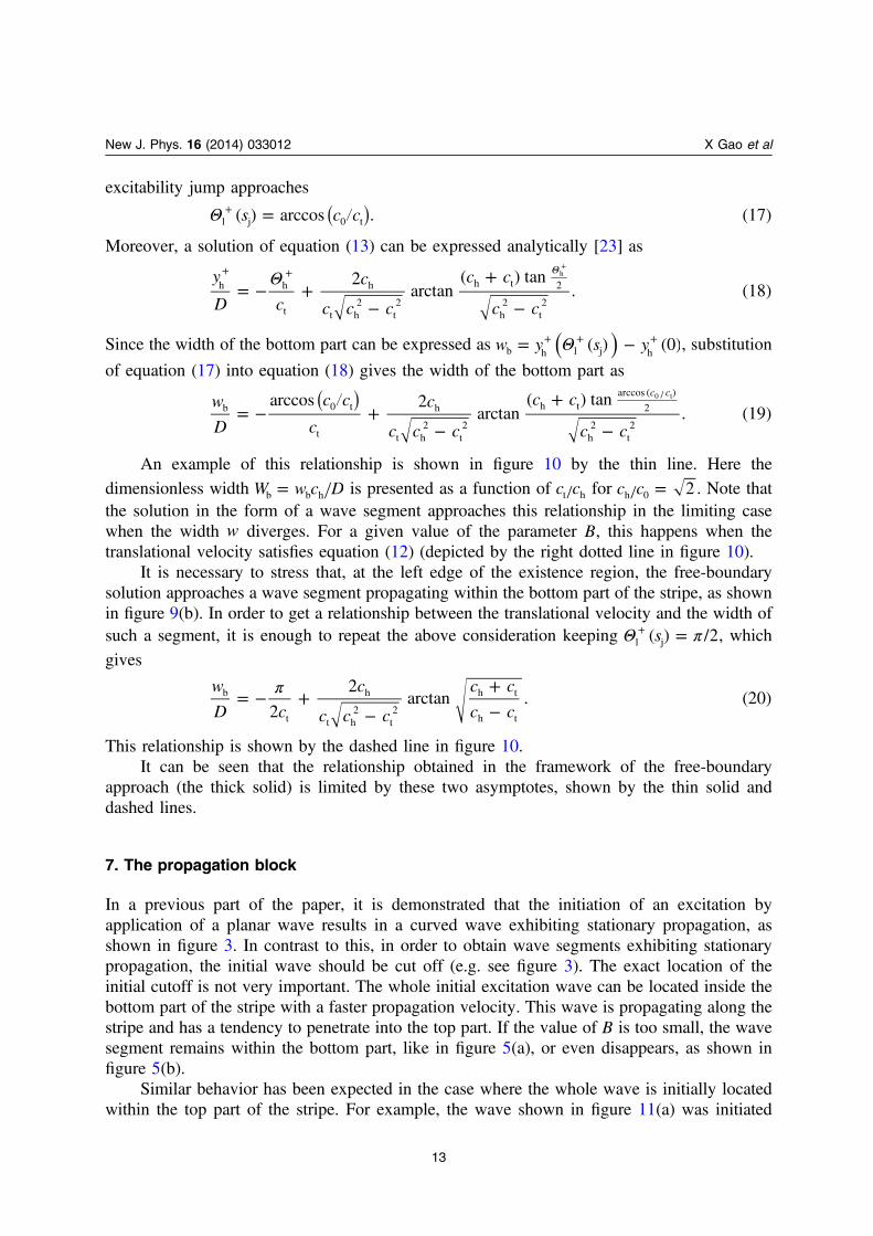
Similar behavior has been expected in the case where the whole wave is initially locatedwithin the top part of the stripe. For example, the wave shown in figure 11(a) was initiated

New J. Phys. 16 (2014) 033012 X Gao et al

13

within the top part and, in the course of time, propagates along the stripe, and penetrates into itsbottom part. Finally, this wave will evolve into a curved wave exhibiting stationary propagationalong the stripe. This dynamics has been observed for <A 1.4h .

However, if the parameter Ah, which determines the propagation velocity in the bottompart, is increased to =A 1.6h , the wave stops penetrating into the bottom part, as shown infigure 11(b). This propagation block looks rather strange because the bottom part is able tosupport traveling waves. Moreover, the propagation velocity here is even larger than that withinthe top part. Hence the bottom part can be considered as more excitable than the top one.

The existence of such a propagation block on the boundary of the propagation velocityjump has also been observed during the numerical computations for 1D excitable media. Theonly small difference is in the critical value of the parameter Ah, i.e. the minimal value for whichthe block takes place.

In order to clarify the reason for this unusual propagation block, let us consider morecarefully the wave pattern in figure 11(b). Note that the bottom boundary of the wave segmentis rather flat. A similar segment shape can be expected if it is induced near a boundary of apassive medium. Such a passive medium can be described using the reaction–diffusion system(1) with the modified kinetic function F u v( , ). Let us take within the bottom part

δ= − − − = −[ ]F u v A u u v v G u v u( , ) 3 ( ) ( ) , ( , ) . (21)h 0 0

The system of equations (1) and (21) has the same steady state as the system (1) and (2)describing the top part. Obviously two-dimensional computations performed with this modifiedkinetics within the bottom part will result in a wave pattern similar to the one shown infigure 11(b). At the boundary between the top and bottom parts, the activator value will reachsome value ub, which will, of course, depend on the parameter Ah. An increase of Ah will reduceub since a negative feedback stabilizing the steady state of the bottom part becomes stronger. Itis clear that for sufficiently large Ah it is possible to get < −u 1.2b . Note that this valuecorresponds to a practically linear part of the nullcline =F u v( , ) 0 shown in figure 2.

New J. Phys. 16 (2014) 033012 X Gao et al

14

35

30

25

20

15

10

5

0

y

35

30

25

20

15

10

5

0y

t=120 t=540

0 10 20 30 40 50 60 70x

0 10 20 30 40 50 60 70x

(a) (b)

Figure 11. Propagation of a wave segment induced in the upper part of the stripe(ε = 0.0005). (a) Wave segment penetrating into the bottom part of the stripe( =A 1.3h ). (b) Propagation of the wave into the bottom part is blocked ( =A 1.6h ).

This means that for such a value of Ah, the kinetic functions in equation (21) can be replaced bythe old ones in equation (2), because the cubic term in equation (2) will be negligibly small.

This is the reason for the observed propagation block. Indeed, if the parameter Ah issufficiently large, the stabilizing negative feedback is so strong that a wave in the top part is notable to exceed the excitation threshold value near the velocity jump line and penetrate into thebottom part. There is an obvious similarity between the observed effect and the propagationblocks in inhomogeneous cardiac tissue, usually referred to as a source–sink mismatch [31].Thus, the propagation block phenomenon discovered could potentially have an application incardiology.

8. Summary

The numerical computations performed with a standard and widely used reaction–diffusionmodel of an excitable medium demonstrate interesting spatiotemporal patterns appearing in aninhomogeneous stripe. Unexpectedly, it is shown that the stationary wave pattern depends onthe initial conditions creating the primary excitation. Application of the free-boundary approachallows us to explain the observed wave patterns. Moreover, the main parameters of the patternsobserved in the reaction–diffusion computations can be predicted in the framework of thisapproach. The accuracy of these predictions is rather high, as can be seen in figure 8. The resultsobtained should be widely applicable to quite different excitable media because the free-boundary approach is based on very general properties of the excitation waves.

The existence of a propagation block on the boundary between two parts of a medium,both of which are supporting excitation waves, is very important for many applications. Forinstance, in cardiology such a phenomenon has to be taken into account as a possiblemechanism of wave breaking leading to cardiac arrhythmia. It can also be used for theengineering of structured excitable media intended for information processing.

Acknowledgments

XG and HZ acknowledge the support of the National Natural Science Foundation of Chinaunder grant no. 11275167.

References

[1] Winfree A T 2000 The Geometry of Biological Time (Berlin: Springer)[2] Mikhailov A S 1994 Foundations of Synergetics (Berlin: Springer)[3] Kapral R and Showalter K (ed) 1995 Chemical Waves and Patterns (Dordrecht: Kluwer)[4] Zykov V S 1987 Simulation of Wave Processes in Excitable Media (Manchester: Manchester University

Press)[5] Jakubith S, Rotermund H H, Engel W, von Oertzen A and Ertel G 1990 Phys. Rev. Lett. 65 3013[6] Zhabotinsky A M and Zaikin A N 1973 J. Theor. Biol. 40 45[7] Gerish G 1971 Naturwissenschaften 58 430[8] Allessie M A, Bonke F I M and Schopman F J G 1973 Circ. Res. 33 54[9] Gorelova N A and Bures J 1983 J. Neurobiol. 14 353

New J. Phys. 16 (2014) 033012 X Gao et al

15

[10] Lechleiter J, Girard S, Peralta E and Clapham D 1991 Science 252 123[11] Hartman N, Bär M, Kevrekidis I G, Krisher K and Imbil R 1996 Phys. Rev. Lett. 76 1384[12] Lewis T J and Keener J P 2000 SIAM J. Appl. Math. 61 293[13] Agladze K, Tóth Á, Ichino T and Yoshikawa K 2000 J. Phys. Chem. A 104 6677[14] Bär M, Meron E and Utzny C 2002 Chaos 12 204[15] Gao X, Feng X, Cai M, Li B, Ying H and Zhang H 2012 Phys. Rev. E 85 016213[16] Liu T-Y and Chang C-H 2013 New J. Phys. 15 035018[17] Jalife J 2000 Ann. Rev. Physiol. 62 25[18] Pumir A, Nikolski V, Höring M, Isomura A, Agladze K, Yoshiokawa K, Gilmour R, Bodenschatz E and

Krinsky V 2007 Phys. Rev. Lett. 99 208101[19] Luther S et al 2011 Nature 475 235[20] Steinbock O, Tóth Á and Schowalter K 1995 Science 267 868[21] Gorecki J, Gorecka J N and Igarashi Y 2009 Nat. Comput. 8 473[22] Zhang G-M, Wong I, Chou M-T and Zhao X 2012 J. Chem. Phys. 136 164108[23] Steinbock O, Zykov V S and Müller S C 1993 Phys. Rev. E 48 3295[24] Zykov V S, Mikhailov A S and Müller S C 1999 Transport and Structure: Their Competitive Roles in

Biophysics and Chemistry (Lecture Notes in Physics vol 532) (Berlin: Springer) p 308[25] Winfree A T 1991 Chaos 1 303[26] Karma A 1991 Phys. Rev. Lett. 66 2274[27] Hakim V and Karma A 1999 Phys. Rev. E 60 5073[28] Zykov V S and Showalter K 2005 Phys. Rev. Lett. 94 068302[29] Kothe A, Zykov V S and Engel H 2009 Phys. Rev. Lett. 103 154102[30] Tyson J J and Keener J P 1988 Physica D 32 327[31] Carmelier E and Vereecke J 2002 Cardiac Cellular Electrophysiology (Dordrecht: Kluwer)

New J. Phys. 16 (2014) 033012 X Gao et al

16