Embed Size (px)
Citation preview

Static Program AnalysisLecture 18: Interprocedural Dataflow Analysis II (Fixpoint Solution)
Summer Semester 2018
Thomas NollSoftware Modeling and Verification GroupRWTH Aachen University
https://moves.rwth-aachen.de/teaching/ss-18/spa/

Recap: Interprocedural Dataflow Analysis
Outline of Lecture 18
Recap: Interprocedural Dataflow Analysis
The Interprocedural Fixpoint Solution
The Equation System
Correctness of Fixpoint Solution
2 of 19 Static Program AnalysisSummer Semester 2018Lecture 18: Interprocedural Dataflow Analysis II (Fixpoint Solution)

Recap: Interprocedural Dataflow Analysis
Extending the Syntax
Syntactic categories:Category Domain Meta variableProcedure identifiers Pid = {P, Q, . . .} PProcedure declarations PDec pCommands (statements) Cmd c
Context-free grammar
p ::= proc [P(val x,res y)]ln is c [end]lx;p | ε ∈ PDecc ::= [skip]l | [x := a]l | c1;c2 | if [b]l then c1 else c2 end |
while [b]l do c end | [call P(a,x)]lclr ∈ Cmd
• All labels and procedure names in program p c distinct• In proc [P(val x,res y)]ln is c [end]lx , ln / lx refers to the entry / exit of P• In [call P(a,x)]lclr , lc / lr refers to the call of / return from P• First parameter call-by-value (input), second call-by-result (output)
3 of 19 Static Program AnalysisSummer Semester 2018Lecture 18: Interprocedural Dataflow Analysis II (Fixpoint Solution)

Recap: Interprocedural Dataflow Analysis
Naive Formulation
• Attempt: directly transfer techniques from intraprocedural analysis=⇒ treat (lc; ln) like (lc, ln) and (lx ; lr ) like (lx , lr )
• Given: dataflow system S = (Lab,E ,F , (D,v), ι, ϕ)
• For each procedure call [call P(a,x)]lclr :transfer functions ϕlc , ϕlr : D → D (definition later)• For each procedure declaration proc [P(val x,res y)]ln is c [end]lx :
transfer functions ϕln, ϕlx : D → D (definition later)• Induces equation system
AIl =
{ι if l ∈ E⊔{ϕl ′(AIl ′) | (l ′, l) ∈ F or (l ′; l) ∈ F} otherwise
• Problem: procedure calls (lc; ln) and procedure returns (lx ; lr ) treated like goto’s=⇒ nesting of calls and returns ignored=⇒ too many paths considered=⇒ analysis information possibly imprecise (but still sound as all “valid” paths covered)
4 of 19 Static Program AnalysisSummer Semester 2018Lecture 18: Interprocedural Dataflow Analysis II (Fixpoint Solution)

Recap: Interprocedural Dataflow Analysis
Valid Paths
• Consider only paths with correct nesting of procedure calls and returns• Yields MVP solution (Meet over all Valid Paths)
Definition (Valid path fragments)
Given a dataflow system S = (Lab,E , F , (D,v), ι, ϕ) and l1, l2 ∈ Lab, the set ofvalid paths from l1 to l2 is generated by the nonterminal symbol P[l1, l2] according tothe following context-free grammar:
P[l1, l2]→ l1 whenever l1 = l2P[l1, l3]→ l1,P[l2, l3] whenever (l1, l2) ∈ FP[lc, l]→ lc,P[ln, lx],P[lr , l] whenever (lc, ln, lx, lr) ∈ iflow
5 of 19 Static Program AnalysisSummer Semester 2018Lecture 18: Interprocedural Dataflow Analysis II (Fixpoint Solution)

Recap: Interprocedural Dataflow Analysis
The MVP Solution I
Definition (Complete valid paths)
Let S = (Lab,E , F , (D,v), ι, ϕ) be a dataflow system. For every l ∈ Lab, the set ofvalid paths up to l is given by
VPath(l) := {[l1, . . . , lk−1] | k ≥ 1, l1 ∈ E , lk = l, [l1, . . . , lk ] valid path from l1 to lk}.For π = [l1, . . . , lk−1] ∈ VPath(l), we define the transfer function ϕπ : D → D by
ϕπ := ϕlk−1 ◦ . . . ◦ ϕl1 ◦ idD
(so that ϕ[] = idD).
6 of 19 Static Program AnalysisSummer Semester 2018Lecture 18: Interprocedural Dataflow Analysis II (Fixpoint Solution)

Recap: Interprocedural Dataflow Analysis
The MVP Solution II
Definition (MVP solution)
Let S = (Lab,E , F , (D,v), ι, ϕ) be a dataflow system where Lab = {l1, . . . , ln}.The MVP solution for S is determined by
mvp(S) := (mvp(l1), . . . ,mvp(ln)) ∈ Dn
where, for every l ∈ Lab,mvp(l) :=
⊔{ϕπ(ι) | π ∈ VPath(l)}.
Corollary
1. mvp(S) v mop(S)
2. The MVP solution is undecidable.
Proof.
1. since VPath(l) ⊆ Path(l) for every l ∈ Lab2. as mvp(S) = mop(S) in intraprocedural case and MOP solution undecidable (Thm. 6.6)
7 of 19 Static Program AnalysisSummer Semester 2018Lecture 18: Interprocedural Dataflow Analysis II (Fixpoint Solution)

The Interprocedural Fixpoint Solution
Outline of Lecture 18
Recap: Interprocedural Dataflow Analysis
The Interprocedural Fixpoint Solution
The Equation System
Correctness of Fixpoint Solution
8 of 19 Static Program AnalysisSummer Semester 2018Lecture 18: Interprocedural Dataflow Analysis II (Fixpoint Solution)

The Interprocedural Fixpoint Solution
The Interprocedural Fixpoint Solution• Goal: adapt fixpoint solution to avoid invalid paths• For simplification: consider only forward problems
• Approach: represent combined effect of procedure execution by procedure summaries(to be used in node transfer function of return label)
⇒ Two types of functions:• Node transfer functions ϕl :
– for non-procedural constructs (skip, assignments, tests): as before (specific to analysis)– for procedure call (lc): parameter passing (specific to analysis)– for procedure entry (ln): initialisation (specific to analysis)– for procedure exit (lx ): always identity– for procedure return (lr ): combine call context with procedure result obtained from summary function
ϕlr (d) = combine(d,Φlx (ϕlc(d)))
(combine specific to analysis)
• Procedure summary functions Φl :– for procedure entry (ln): identity– for procedure exit (lx ): full effect– inductively defined by stepwise composition of node transfer functions
9 of 19 Static Program AnalysisSummer Semester 2018Lecture 18: Interprocedural Dataflow Analysis II (Fixpoint Solution)

The Interprocedural Fixpoint Solution
The Interprocedural Fixpoint Solution• Goal: adapt fixpoint solution to avoid invalid paths• For simplification: consider only forward problems• Approach: represent combined effect of procedure execution by procedure summaries
(to be used in node transfer function of return label)
⇒ Two types of functions:• Node transfer functions ϕl :
– for non-procedural constructs (skip, assignments, tests): as before (specific to analysis)– for procedure call (lc): parameter passing (specific to analysis)– for procedure entry (ln): initialisation (specific to analysis)– for procedure exit (lx ): always identity– for procedure return (lr ): combine call context with procedure result obtained from summary function
ϕlr (d) = combine(d,Φlx (ϕlc(d)))
(combine specific to analysis)
• Procedure summary functions Φl :– for procedure entry (ln): identity– for procedure exit (lx ): full effect– inductively defined by stepwise composition of node transfer functions
9 of 19 Static Program AnalysisSummer Semester 2018Lecture 18: Interprocedural Dataflow Analysis II (Fixpoint Solution)

The Interprocedural Fixpoint Solution
The Interprocedural Fixpoint Solution• Goal: adapt fixpoint solution to avoid invalid paths• For simplification: consider only forward problems• Approach: represent combined effect of procedure execution by procedure summaries
(to be used in node transfer function of return label)⇒ Two types of functions:• Node transfer functions ϕl :
– for non-procedural constructs (skip, assignments, tests): as before (specific to analysis)– for procedure call (lc): parameter passing (specific to analysis)– for procedure entry (ln): initialisation (specific to analysis)– for procedure exit (lx ): always identity– for procedure return (lr ): combine call context with procedure result obtained from summary function
ϕlr (d) = combine(d,Φlx (ϕlc(d)))
(combine specific to analysis)
• Procedure summary functions Φl :– for procedure entry (ln): identity– for procedure exit (lx ): full effect– inductively defined by stepwise composition of node transfer functions
9 of 19 Static Program AnalysisSummer Semester 2018Lecture 18: Interprocedural Dataflow Analysis II (Fixpoint Solution)

The Interprocedural Fixpoint Solution
Procedure Summaries
[P(val x,res y)]ln Φln = idD
[. . .]l1 Φl1 = ϕln
[. . .]l2 Φl2 = ϕl1 ◦ ϕln = Φl3 [. . .]l3
[end]lx Φlx = ϕl2 ◦ ϕl1 ◦ ϕln t ϕl3 ◦ ϕl1 ◦ ϕln
10 of 19 Static Program AnalysisSummer Semester 2018Lecture 18: Interprocedural Dataflow Analysis II (Fixpoint Solution)

The Interprocedural Fixpoint Solution
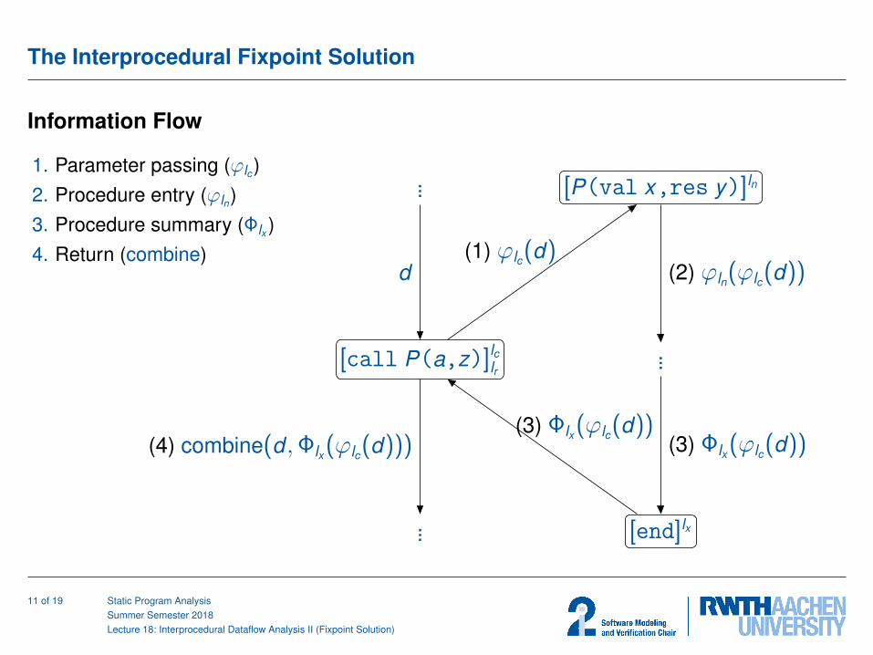
Information Flow
1. Parameter passing (ϕlc)2. Procedure entry (ϕln)3. Procedure summary (Φlx )4. Return (combine)
...
[call P(a,z)]lclr
...
[P(val x,res y)]ln
...
[end]lx
11 of 19 Static Program AnalysisSummer Semester 2018Lecture 18: Interprocedural Dataflow Analysis II (Fixpoint Solution)

The Interprocedural Fixpoint Solution
Information Flow
1. Parameter passing (ϕlc)
2. Procedure entry (ϕln)3. Procedure summary (Φlx )4. Return (combine)
...
[call P(a,z)]lclr
...
[P(val x,res y)]ln
...
[end]lx
d(1) ϕlc(d)
11 of 19 Static Program AnalysisSummer Semester 2018Lecture 18: Interprocedural Dataflow Analysis II (Fixpoint Solution)

The Interprocedural Fixpoint Solution
Information Flow
1. Parameter passing (ϕlc)2. Procedure entry (ϕln)
3. Procedure summary (Φlx )4. Return (combine)
...
[call P(a,z)]lclr
...
[P(val x,res y)]ln
...
[end]lx
d(1) ϕlc(d)
(2) ϕln(ϕlc(d))
11 of 19 Static Program AnalysisSummer Semester 2018Lecture 18: Interprocedural Dataflow Analysis II (Fixpoint Solution)

The Interprocedural Fixpoint Solution
Information Flow
1. Parameter passing (ϕlc)2. Procedure entry (ϕln)3. Procedure summary (Φlx )
4. Return (combine)
...
[call P(a,z)]lclr
...
[P(val x,res y)]ln
...
[end]lx
d(1) ϕlc(d)
(2) ϕln(ϕlc(d))
(3) Φlx (ϕlc(d))(3) Φlx (ϕlc(d))
11 of 19 Static Program AnalysisSummer Semester 2018Lecture 18: Interprocedural Dataflow Analysis II (Fixpoint Solution)
The Interprocedural Fixpoint Solution
Information Flow
1. Parameter passing (ϕlc)2. Procedure entry (ϕln)3. Procedure summary (Φlx )4. Return (combine)
...
[call P(a,z)]lclr
...
[P(val x,res y)]ln
...
[end]lx
d(1) ϕlc(d)
(2) ϕln(ϕlc(d))
(3) Φlx (ϕlc(d))(3) Φlx (ϕlc(d))
(4) combine(d ,Φlx (ϕlc(d)))
11 of 19 Static Program AnalysisSummer Semester 2018Lecture 18: Interprocedural Dataflow Analysis II (Fixpoint Solution)

The Interprocedural Fixpoint Solution
Example: Constant Propagation
Example 18.1 (Constant Propagation; cf. Lecture 5/6)
S := (Lab,E , F , (D,v), ι, ϕ,Φ) is determined by• D := {δ | δ : Var c → Z ∪ {⊥,>}} (constant/undefined/overdefined)• ⊥ v z v > for every z ∈ Z• ι := δ> ∈ D• For each l ∈ Lab \ {lc, ln, lx , lr | (lc, ln, lx , lr ) ∈ iflow},
ϕl(δ) :=
{δ if Bl = skip or Bl ∈ BExpδ[x 7→ valδ(a)] if Bl = (x := a)
• Whenever p c contains [call P(a,z)]lclr and proc [P(val x,res y)]ln is c [end]lx :– call/entry: set input and reset output parameter
ϕlc(δ) := δ[x 7→ valδ(a), y 7→ >], ϕln(δ) := δ
– return: reset parameters (x, y possibly used in calling context) and set return value
ϕlr (δ) := combine(δ,Φlx (ϕlc(δ))), combine(δ, δ′) := δ′[x 7→ δ(x), y 7→ δ(y), z 7→ δ′(y)]
(note: order of δ′ updates important in case z ∈ {x, y}; definition of Φ: later)
12 of 19 Static Program AnalysisSummer Semester 2018Lecture 18: Interprocedural Dataflow Analysis II (Fixpoint Solution)

The Equation System
Outline of Lecture 18
Recap: Interprocedural Dataflow Analysis
The Interprocedural Fixpoint Solution
The Equation System
Correctness of Fixpoint Solution
13 of 19 Static Program AnalysisSummer Semester 2018Lecture 18: Interprocedural Dataflow Analysis II (Fixpoint Solution)

The Equation System
Types of Equations
For an interprocedural dataflow system S := (Lab,E , F , (D,v), ι, ϕ,Φ) theintraprocedural equation system (cf. Definition 4.3)
AIl =
{ι if l ∈ E⊔{ϕl ′(AIl ′) | (l ′, l) ∈ F} otherwise
is extended to a system with three kinds of equations (for l ∈ Lab):
• for actual dataflow information: AIl ∈ D– counterpart of intraprocedural AI
• for node transfer functions: ϕl : D → D– extension of intraprocedural transfer functions by handling of procedure calls
• for procedure summary functions of complete procedures: Φl : D → D– Φl(d) yields information at (entry of) l if corresponding procedure is called with information d– thus Φln(d) = d and complete procedure effect represented by Φlx (d)
14 of 19 Static Program AnalysisSummer Semester 2018Lecture 18: Interprocedural Dataflow Analysis II (Fixpoint Solution)

The Equation System
Types of Equations
For an interprocedural dataflow system S := (Lab,E , F , (D,v), ι, ϕ,Φ) theintraprocedural equation system (cf. Definition 4.3)
AIl =
{ι if l ∈ E⊔{ϕl ′(AIl ′) | (l ′, l) ∈ F} otherwise
is extended to a system with three kinds of equations (for l ∈ Lab):• for actual dataflow information: AIl ∈ D
– counterpart of intraprocedural AI
• for node transfer functions: ϕl : D → D– extension of intraprocedural transfer functions by handling of procedure calls
• for procedure summary functions of complete procedures: Φl : D → D– Φl(d) yields information at (entry of) l if corresponding procedure is called with information d– thus Φln(d) = d and complete procedure effect represented by Φlx (d)
14 of 19 Static Program AnalysisSummer Semester 2018Lecture 18: Interprocedural Dataflow Analysis II (Fixpoint Solution)

The Equation System
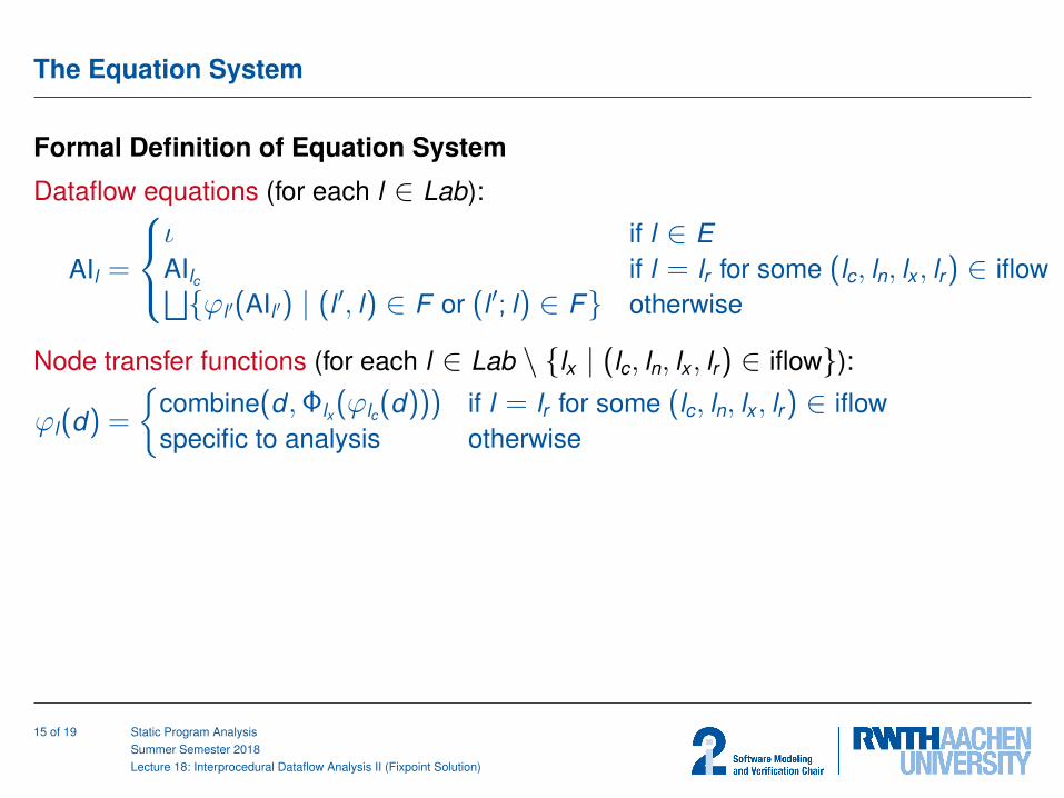
Formal Definition of Equation System
Dataflow equations (for each l ∈ Lab):
AIl =
ι if l ∈ EAIlc if l = lr for some (lc, ln, lx, lr) ∈ iflow⊔{ϕl ′(AIl ′) | (l ′, l) ∈ F or (l ′; l) ∈ F} otherwise
Node transfer functions (for each l ∈ Lab \ {lx | (lc, ln, lx, lr) ∈ iflow}):
ϕl(d) =
{combine(d ,Φlx (ϕlc(d))) if l = lr for some (lc, ln, lx, lr) ∈ iflowspecific to analysis otherwise
Procedure summary functions (for each l ∈ Lab occurring in some procedure):
Φl(d) =
d if l = ln for some (lc, ln, lx, lr) ∈ iflowΦlc(d) if l = lr for some (lc, ln, lx, lr) ∈ iflow⊔{ϕl ′(Φl ′(d)) | (l ′, l) ∈ F} otherwise
Note: introduces recursive equations for AIl (of type D) and Φl (of type D → D)
15 of 19 Static Program AnalysisSummer Semester 2018Lecture 18: Interprocedural Dataflow Analysis II (Fixpoint Solution)
The Equation System
Formal Definition of Equation System
Dataflow equations (for each l ∈ Lab):
AIl =
ι if l ∈ EAIlc if l = lr for some (lc, ln, lx, lr) ∈ iflow⊔{ϕl ′(AIl ′) | (l ′, l) ∈ F or (l ′; l) ∈ F} otherwise
Node transfer functions (for each l ∈ Lab \ {lx | (lc, ln, lx, lr) ∈ iflow}):
ϕl(d) =
{combine(d ,Φlx (ϕlc(d))) if l = lr for some (lc, ln, lx, lr) ∈ iflowspecific to analysis otherwise
Procedure summary functions (for each l ∈ Lab occurring in some procedure):
Φl(d) =
d if l = ln for some (lc, ln, lx, lr) ∈ iflowΦlc(d) if l = lr for some (lc, ln, lx, lr) ∈ iflow⊔{ϕl ′(Φl ′(d)) | (l ′, l) ∈ F} otherwise
Note: introduces recursive equations for AIl (of type D) and Φl (of type D → D)
15 of 19 Static Program AnalysisSummer Semester 2018Lecture 18: Interprocedural Dataflow Analysis II (Fixpoint Solution)

The Equation System
Solving the Equation System• Monotonicity of ϕl implies monotonicity of Φl ′ (Φl ′ : D →mon D)
• Complete lattice property of (D,v) ensures that (D →mon D, v) is complete lattice– Φ1vΦ2 iff ∀d ∈ D : Φ1(d) v Φ2(d) (pointwise extension)
• Equation system induces monotonic functional on complete latticeΨS : Dn︸︷︷︸
AI
× (D →mon D)m︸ ︷︷ ︸Φ
→ Dn × (D →mon D)m
where n = |Lab| and m ≤ n (procedure labels)• Thus least solution effectively computable by fixpoint iteration (Theorem 3.15):
fix(ΨS) =⊔{Ψk
S(⊥) | k ∈ N} ∈ Dn × (D →mon D)m
where ⊥ = (⊥nD, [d 7→ ⊥D | d ∈ D]m)
• Moreover:– (D →mon D, v) satisfies ACC if (D,v) satisfies ACC– Φl ′ distributive if ϕl distributive
• Problem: effective and efficient representation of procedure summaries– D finite =⇒ D →mon D finite =⇒ can use (compact representation of) value tables– often: demand-driven approach (restrict analysis to values occurring in calls)– example: Constant Propagation (see following slide)
16 of 19 Static Program AnalysisSummer Semester 2018Lecture 18: Interprocedural Dataflow Analysis II (Fixpoint Solution)

The Equation System
Solving the Equation System• Monotonicity of ϕl implies monotonicity of Φl ′ (Φl ′ : D →mon D)• Complete lattice property of (D,v) ensures that (D →mon D, v) is complete lattice
– Φ1vΦ2 iff ∀d ∈ D : Φ1(d) v Φ2(d) (pointwise extension)
• Equation system induces monotonic functional on complete latticeΨS : Dn︸︷︷︸
AI
× (D →mon D)m︸ ︷︷ ︸Φ
→ Dn × (D →mon D)m
where n = |Lab| and m ≤ n (procedure labels)• Thus least solution effectively computable by fixpoint iteration (Theorem 3.15):
fix(ΨS) =⊔{Ψk
S(⊥) | k ∈ N} ∈ Dn × (D →mon D)m
where ⊥ = (⊥nD, [d 7→ ⊥D | d ∈ D]m)
• Moreover:– (D →mon D, v) satisfies ACC if (D,v) satisfies ACC– Φl ′ distributive if ϕl distributive
• Problem: effective and efficient representation of procedure summaries– D finite =⇒ D →mon D finite =⇒ can use (compact representation of) value tables– often: demand-driven approach (restrict analysis to values occurring in calls)– example: Constant Propagation (see following slide)
16 of 19 Static Program AnalysisSummer Semester 2018Lecture 18: Interprocedural Dataflow Analysis II (Fixpoint Solution)

The Equation System
Solving the Equation System• Monotonicity of ϕl implies monotonicity of Φl ′ (Φl ′ : D →mon D)• Complete lattice property of (D,v) ensures that (D →mon D, v) is complete lattice
– Φ1vΦ2 iff ∀d ∈ D : Φ1(d) v Φ2(d) (pointwise extension)• Equation system induces monotonic functional on complete lattice
ΨS : Dn︸︷︷︸AI
× (D →mon D)m︸ ︷︷ ︸Φ
→ Dn × (D →mon D)m
where n = |Lab| and m ≤ n (procedure labels)
• Thus least solution effectively computable by fixpoint iteration (Theorem 3.15):
fix(ΨS) =⊔{Ψk
S(⊥) | k ∈ N} ∈ Dn × (D →mon D)m
where ⊥ = (⊥nD, [d 7→ ⊥D | d ∈ D]m)
• Moreover:– (D →mon D, v) satisfies ACC if (D,v) satisfies ACC– Φl ′ distributive if ϕl distributive
• Problem: effective and efficient representation of procedure summaries– D finite =⇒ D →mon D finite =⇒ can use (compact representation of) value tables– often: demand-driven approach (restrict analysis to values occurring in calls)– example: Constant Propagation (see following slide)
16 of 19 Static Program AnalysisSummer Semester 2018Lecture 18: Interprocedural Dataflow Analysis II (Fixpoint Solution)

The Equation System
Solving the Equation System• Monotonicity of ϕl implies monotonicity of Φl ′ (Φl ′ : D →mon D)• Complete lattice property of (D,v) ensures that (D →mon D, v) is complete lattice
– Φ1vΦ2 iff ∀d ∈ D : Φ1(d) v Φ2(d) (pointwise extension)• Equation system induces monotonic functional on complete lattice
ΨS : Dn︸︷︷︸AI
× (D →mon D)m︸ ︷︷ ︸Φ
→ Dn × (D →mon D)m
where n = |Lab| and m ≤ n (procedure labels)• Thus least solution effectively computable by fixpoint iteration (Theorem 3.15):
fix(ΨS) =⊔{Ψk
S(⊥) | k ∈ N} ∈ Dn × (D →mon D)m
where ⊥ = (⊥nD, [d 7→ ⊥D | d ∈ D]m)
• Moreover:– (D →mon D, v) satisfies ACC if (D,v) satisfies ACC– Φl ′ distributive if ϕl distributive
• Problem: effective and efficient representation of procedure summaries– D finite =⇒ D →mon D finite =⇒ can use (compact representation of) value tables– often: demand-driven approach (restrict analysis to values occurring in calls)– example: Constant Propagation (see following slide)
16 of 19 Static Program AnalysisSummer Semester 2018Lecture 18: Interprocedural Dataflow Analysis II (Fixpoint Solution)

The Equation System
Solving the Equation System• Monotonicity of ϕl implies monotonicity of Φl ′ (Φl ′ : D →mon D)• Complete lattice property of (D,v) ensures that (D →mon D, v) is complete lattice
– Φ1vΦ2 iff ∀d ∈ D : Φ1(d) v Φ2(d) (pointwise extension)• Equation system induces monotonic functional on complete lattice
ΨS : Dn︸︷︷︸AI
× (D →mon D)m︸ ︷︷ ︸Φ
→ Dn × (D →mon D)m
where n = |Lab| and m ≤ n (procedure labels)• Thus least solution effectively computable by fixpoint iteration (Theorem 3.15):
fix(ΨS) =⊔{Ψk
S(⊥) | k ∈ N} ∈ Dn × (D →mon D)m
where ⊥ = (⊥nD, [d 7→ ⊥D | d ∈ D]m)
• Moreover:– (D →mon D, v) satisfies ACC if (D,v) satisfies ACC– Φl ′ distributive if ϕl distributive
• Problem: effective and efficient representation of procedure summaries– D finite =⇒ D →mon D finite =⇒ can use (compact representation of) value tables– often: demand-driven approach (restrict analysis to values occurring in calls)– example: Constant Propagation (see following slide)
16 of 19 Static Program AnalysisSummer Semester 2018Lecture 18: Interprocedural Dataflow Analysis II (Fixpoint Solution)

The Equation System
Example of Equation System
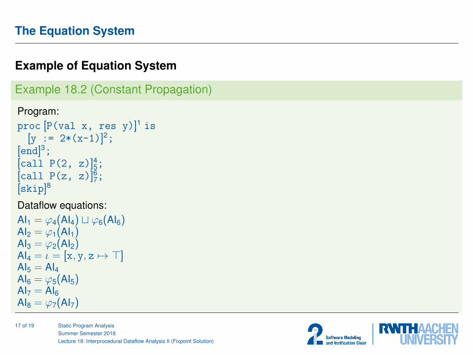
Example 18.2 (Constant Propagation)
Program:proc [P(val x, res y)]1 is
[y := 2*(x-1)]2;[end]3;[call P(2, z)]4
5;[call P(z, z)]6
7;[skip]8
Dataflow equations:AI1 = ϕ4(AI4) t ϕ6(AI6)AI2 = ϕ1(AI1)AI3 = ϕ2(AI2)AI4 = ι = [x, y, z 7→ >]AI5 = AI4AI6 = ϕ5(AI5)AI7 = AI6AI8 = ϕ7(AI7)
Node transfer functions:ϕ1(δ) = δϕ2(δ) = δ[y 7→ valδ(2*(x-1))]ϕ4(δ) = δ[x 7→ 2, y 7→ >]ϕ5(δ) = combine(δ,Φ3(ϕ4(δ)))ϕ6(δ) = δ[x 7→ δ(z), y 7→ >]ϕ7(δ) = combine(δ,Φ3(ϕ6(δ)))
combine(δ, δ′) = δ′[x 7→ δ(x), y 7→ δ(y), z 7→ δ′(y)]Procedure summary functions:Φ1(δ) = δΦ2(δ) = ϕ1(Φ1(δ)) = δΦ3(δ) = ϕ2(Φ2(δ)) = δ[y 7→ valδ(2*(x-1))]
Fixpoint iteration: on the board
17 of 19 Static Program AnalysisSummer Semester 2018Lecture 18: Interprocedural Dataflow Analysis II (Fixpoint Solution)
The Equation System
Example of Equation System
Example 18.2 (Constant Propagation)
Program:proc [P(val x, res y)]1 is
[y := 2*(x-1)]2;[end]3;[call P(2, z)]4
5;[call P(z, z)]6
7;[skip]8
Dataflow equations:AI1 = ϕ4(AI4) t ϕ6(AI6)AI2 = ϕ1(AI1)AI3 = ϕ2(AI2)AI4 = ι = [x, y, z 7→ >]AI5 = AI4AI6 = ϕ5(AI5)AI7 = AI6AI8 = ϕ7(AI7)
Node transfer functions:ϕ1(δ) = δϕ2(δ) = δ[y 7→ valδ(2*(x-1))]ϕ4(δ) = δ[x 7→ 2, y 7→ >]ϕ5(δ) = combine(δ,Φ3(ϕ4(δ)))ϕ6(δ) = δ[x 7→ δ(z), y 7→ >]ϕ7(δ) = combine(δ,Φ3(ϕ6(δ)))
combine(δ, δ′) = δ′[x 7→ δ(x), y 7→ δ(y), z 7→ δ′(y)]Procedure summary functions:Φ1(δ) = δΦ2(δ) = ϕ1(Φ1(δ)) = δΦ3(δ) = ϕ2(Φ2(δ)) = δ[y 7→ valδ(2*(x-1))]
Fixpoint iteration: on the board
17 of 19 Static Program AnalysisSummer Semester 2018Lecture 18: Interprocedural Dataflow Analysis II (Fixpoint Solution)

The Equation System
Example of Equation System
Example 18.2 (Constant Propagation)
Program:proc [P(val x, res y)]1 is
[y := 2*(x-1)]2;[end]3;[call P(2, z)]4
5;[call P(z, z)]6
7;[skip]8
Dataflow equations:AI1 = ϕ4(AI4) t ϕ6(AI6)AI2 = ϕ1(AI1)AI3 = ϕ2(AI2)AI4 = ι = [x, y, z 7→ >]AI5 = AI4AI6 = ϕ5(AI5)AI7 = AI6AI8 = ϕ7(AI7)
Node transfer functions:ϕ1(δ) = δϕ2(δ) = δ[y 7→ valδ(2*(x-1))]ϕ4(δ) = δ[x 7→ 2, y 7→ >]ϕ5(δ) = combine(δ,Φ3(ϕ4(δ)))ϕ6(δ) = δ[x 7→ δ(z), y 7→ >]ϕ7(δ) = combine(δ,Φ3(ϕ6(δ)))
combine(δ, δ′) = δ′[x 7→ δ(x), y 7→ δ(y), z 7→ δ′(y)]
Procedure summary functions:Φ1(δ) = δΦ2(δ) = ϕ1(Φ1(δ)) = δΦ3(δ) = ϕ2(Φ2(δ)) = δ[y 7→ valδ(2*(x-1))]
Fixpoint iteration: on the board
17 of 19 Static Program AnalysisSummer Semester 2018Lecture 18: Interprocedural Dataflow Analysis II (Fixpoint Solution)

The Equation System
Example of Equation System
Example 18.2 (Constant Propagation)
Program:proc [P(val x, res y)]1 is
[y := 2*(x-1)]2;[end]3;[call P(2, z)]4
5;[call P(z, z)]6
7;[skip]8
Dataflow equations:AI1 = ϕ4(AI4) t ϕ6(AI6)AI2 = ϕ1(AI1)AI3 = ϕ2(AI2)AI4 = ι = [x, y, z 7→ >]AI5 = AI4AI6 = ϕ5(AI5)AI7 = AI6AI8 = ϕ7(AI7)
Node transfer functions:ϕ1(δ) = δϕ2(δ) = δ[y 7→ valδ(2*(x-1))]ϕ4(δ) = δ[x 7→ 2, y 7→ >]ϕ5(δ) = combine(δ,Φ3(ϕ4(δ)))ϕ6(δ) = δ[x 7→ δ(z), y 7→ >]ϕ7(δ) = combine(δ,Φ3(ϕ6(δ)))
combine(δ, δ′) = δ′[x 7→ δ(x), y 7→ δ(y), z 7→ δ′(y)]Procedure summary functions:Φ1(δ) = δΦ2(δ) = ϕ1(Φ1(δ)) = δΦ3(δ) = ϕ2(Φ2(δ)) = δ[y 7→ valδ(2*(x-1))]
Fixpoint iteration: on the board
17 of 19 Static Program AnalysisSummer Semester 2018Lecture 18: Interprocedural Dataflow Analysis II (Fixpoint Solution)

The Equation System
Example of Equation System
Example 18.2 (Constant Propagation)
Program:proc [P(val x, res y)]1 is
[y := 2*(x-1)]2;[end]3;[call P(2, z)]4
5;[call P(z, z)]6
7;[skip]8
Dataflow equations:AI1 = ϕ4(AI4) t ϕ6(AI6)AI2 = ϕ1(AI1)AI3 = ϕ2(AI2)AI4 = ι = [x, y, z 7→ >]AI5 = AI4AI6 = ϕ5(AI5)AI7 = AI6AI8 = ϕ7(AI7)
Node transfer functions:ϕ1(δ) = δϕ2(δ) = δ[y 7→ valδ(2*(x-1))]ϕ4(δ) = δ[x 7→ 2, y 7→ >]ϕ5(δ) = combine(δ,Φ3(ϕ4(δ)))ϕ6(δ) = δ[x 7→ δ(z), y 7→ >]ϕ7(δ) = combine(δ,Φ3(ϕ6(δ)))
combine(δ, δ′) = δ′[x 7→ δ(x), y 7→ δ(y), z 7→ δ′(y)]Procedure summary functions:Φ1(δ) = δΦ2(δ) = ϕ1(Φ1(δ)) = δΦ3(δ) = ϕ2(Φ2(δ)) = δ[y 7→ valδ(2*(x-1))]
Fixpoint iteration: on the board
17 of 19 Static Program AnalysisSummer Semester 2018Lecture 18: Interprocedural Dataflow Analysis II (Fixpoint Solution)

Correctness of Fixpoint Solution
Outline of Lecture 18
Recap: Interprocedural Dataflow Analysis
The Interprocedural Fixpoint Solution
The Equation System
Correctness of Fixpoint Solution
18 of 19 Static Program AnalysisSummer Semester 2018Lecture 18: Interprocedural Dataflow Analysis II (Fixpoint Solution)

Correctness of Fixpoint Solution
Soundness and Completeness
The following results carry over from the intraprocedural case:
Theorem 18.3
Let S := (Lab,E , F , (D,v), ι, ϕ) be a dataflow system with interproceduralextension S := (Lab,E , F , (D,v), ι, ϕ,Φ) with MVP solution mvp(S) (Def. 17.9)and fixpoint solution fix(ΨS) = (d1, . . . , dn, f1, . . . , fm). Then:1. (cf. Theorem 6.2)
mvp(S) vn (d1, . . . , dn)
2. (cf. Theorem 6.5)mvp(S) = (d1, . . . , dn) if all ϕl are distributive
Proof.
see J. Knoop, B. Steffen: The Interprocedural Coincidence Theorem, Proc. CC ’92,LNCS 641, Springer, 1992, 125–1401
1https://link.springer.com/chapter/10.1007/3-540-55984-1_13
19 of 19 Static Program AnalysisSummer Semester 2018Lecture 18: Interprocedural Dataflow Analysis II (Fixpoint Solution)
![moves.rwth-aachen.de · Reducing ∞-SafetytoT-Safety SynthesizingStochasticBCs ExperimentalResults ConcludingRemarks. ApplicationsofStochasticDifferentialDynamics ©[PNGGuru] Windforces](https://img.pdfslide.us/doc/110x75/5f7b56f1d1e17c7268721be5/movesrwth-reducing-a-safetytot-safety-synthesizingstochasticbcs-experimentalresults.jpg)