Embed Size (px)
Citation preview

THESIS FOR THE DEGREE OFDOCTOR OFPHILOSOPHY
Static-priority scheduling on multiprocessors
BJORN ANDERSSON
Department of Computer EngineeringCHALMERS UNIVERSITY OF TECHNOLOGY
Goteborg, Sweden 2003

Static-priority scheduling on multiprocessorsBJORN ANDERSSONISBN 91-7291-322-3
c BJORN ANDERSSON, 2003.
Doktorsavhandlingar vid Chalmers tekniska hogskolaNy serie Nr 2004ISSN 0346-718X
School of Computer Science and EngineeringChalmers University of TechnologyTechnical report 17D
Department of Computer EngineeringChalmers University of TechnologySE–412 96 GoteborgSwedenTelephone: + 46 (0)31–772 1000www.ce.chalmers.se
Author email address:[email protected]
Printed by Chalmers ReproserviceGoteborg, Sweden 2003

i
Static-priority scheduling on multiprocessors
BJORN ANDERSSONDepartment of Computer EngineeringChalmers University of Technology
Abstract
This thesis deals with the problem of scheduling a set of tasks to meet deadlines on acomputer with multiple processors. Static-priority scheduling is considered, that is, atask is assigned a priority number that never changes and at every moment the highest-priority tasks that request to be executed are selected for execution.
The performance metric used is the capacity that tasks can request without missinga deadline. It is shown that every static-priority algorithm can miss deadlines althoughclose to 50% of the capacity is requested. The new algorithms in this thesis have thefollowing performance. In periodic scheduling, the capacity that can be requested with-out missing a deadline is: 33% for migrative scheduling and 50% for non-migrativescheduling. In aperiodic scheduling, many performance metrics have been used in pre-vious research. With the aperiodic model used in this thesis, the new algorithms inthis thesis have the following performance. The capacity that can be requested with-out missing a deadline is: 50% for migrative scheduling and 31% for non-migrativescheduling.
Keywords: real-time systems, real-time scheduling, multiprocessors, multiprocessorscheduling, static-priority scheduling, global scheduling, partitioned scheduling, peri-odic, aperiodic, online scheduling.

ii

List of papers
List of Papers
This thesis is based on and extends the work and results presented in the followingpapers and publications:
I . Bjorn Andersson and Jan Jonsson, “Fixed-Priority Preemptive MultiprocessorScheduling: To Partition or Not to Partition,” InProc. of the InternationalConference on Real-Time Computing Systems and Applications, pages 337–346,Cheju Island, Korea, December 12–14, 2000.
II . Bjorn Andersson and Jan Jonsson,“Some Insights on Fixed-Priority PreemptiveNon-Partitioned Multiprocessor Scheduling,”Technical Report no. 01–2, De-partment of Computer Engineering, Chalmers University of Technology, Swe-den, 2001.
III . Bjorn Andersson, Sanjoy Baruah and Jan Jonsson, “Static-Priority Schedulingon Multiprocessors,” InProc. of the IEEE Real-Time Systems Symposium, pages193-202, London, UK, December 3–6, 2001.
IV . Bjorn Andersson and Jan Jonsson, “Preemptive Multiprocessor SchedulingAnomalies,” InProc. of the International Parallel and Distributed ProcessingSymposium, pages 12–19, Fort Lauderdale, Florida, April 15–19, 2002.
V. Bjorn Andersson, Tarek Abdelzaher and Jan Jonsson, “Global Priority-DrivenAperiodic Scheduling on Multiprocessors,” InProc. of the International Paralleland Distributed Processing Symposium, Nice, France, April 22–26, 2003.
VI . Bjorn Andersson, Tarek Abdelzaher and Jan Jonsson, “Partitioned AperiodicScheduling on Multiprocessors,” InProc. of the International Parallel and Dis-tributed Processing Symposium, Nice, France, April 22–26, 2003.
VII . Bjorn Andersson and Jan Jonsson, “The utilization bounds of partitioned andpfair static-priority scheduling on multiprocessors are 50%,” InProc. of theEuromicro Conference on Real-Time Systems, pages 33–40, Porto, Portugal, July2–4, 2003.
iii

iv LIST OF PAPERS
The following papers and publications are related but not covered in this thesis:
I . Tarek Abdelzaher, Bjorn Andersson, Jan Jonsson, Vivek Sharma and MinhNguyen, “The Aperiodic Multiprocessor Utilization Bound for Liquid Tasks,” InReal-Time Technology and Applications Symposium, pages 173–185, San Jose,California, September 24–27, 2002.
II . Vivek Sharma, Tarek Abdelzaher, Bjorn Andersson, Shiva Prasad, Qiuhua Cao,“Generalized Utilization-Based Aperiodic Schedulability Analysis for LiquidTasks,”Technical Report at Department of Computer Science, University of Vir-ginia, 2002.

Contents
1 Introduction 11.1 Real-time systems . . . . . . . . . . . . . . . . . . . . . . . . . . . . . 3
1.1.1 Real-time requirements . . . . . . . . . . . . . . . . . . . . . . 31.1.2 Satisfying real-time requirements . . . . . . . . . . . . . . . . 41.1.3 Verifying real-time requirements . . . . . . . . . . . . . . . . . 6
1.2 Design space of scheduling algorithms . . . . . . . . . . . . . . . . . . 71.3 Problems, assumptions and related work . . . . . . . . . . . . . . . . . 9
1.3.1 Problem statement . . . . . . . . . . . . . . . . . . . . . . . . 91.3.2 Assumptions . . . . . . . . . . . . . . . . . . . . . . . . . . . 101.3.3 Related work . . . . . . . . . . . . . . . . . . . . . . . . . . . 11
1.4 Thesis contributions . . . . . . . . . . . . . . . . . . . . . . . . . . . . 131.5 Thesis outline . . . . . . . . . . . . . . . . . . . . . . . . . . . . . . . 14
I Periodic scheduling 15
2 Introduction to periodic scheduling 172.1 Motivation . . . . . . . . . . . . . . . . . . . . . . . . . . . . . . . . . 172.2 System model . . . . . . . . . . . . . . . . . . . . . . . . . . . . . . . 172.3 Design issues in periodic scheduling . . . . . . . . . . . . . . . . . . . 19
2.3.1 Uniprocessor scheduling . . . . . . . . . . . . . . . . . . . . . 192.3.2 Partitioned scheduling . . . . . . . . . . . . . . . . . . . . . . 222.3.3 Global scheduling . . . . . . . . . . . . . . . . . . . . . . . . 23
2.4 Detailed contributions . . . . . . . . . . . . . . . . . . . . . . . . . . . 25
3 Global scheduling 293.1 Introduction . . . . . . . . . . . . . . . . . . . . . . . . . . . . . . . . 293.2 Results we will use . . . . . . . . . . . . . . . . . . . . . . . . . . . . 303.3 AlgorithmRM-US(m/(3m-2)) . . . . . . . . . . . . . . . . . . . . . . 32
3.3.1 “Light” systems . . . . . . . . . . . . . . . . . . . . . . . . . . 323.3.2 Arbitrary systems . . . . . . . . . . . . . . . . . . . . . . . . . 37
v

vi CONTENTS
3.4 Bound on utilization bounds . . . . . . . . . . . . . . . . . . . . . . . 39
4 Partitioned scheduling 414.1 Introduction . . . . . . . . . . . . . . . . . . . . . . . . . . . . . . . . 414.2 Background on partitioned scheduling . . . . . . . . . . . . . . . . . . 414.3 Restricted periods . . . . . . . . . . . . . . . . . . . . . . . . . . . . . 434.4 Not restricted periods . . . . . . . . . . . . . . . . . . . . . . . . . . . 49
5 Anomalies 515.1 Introduction . . . . . . . . . . . . . . . . . . . . . . . . . . . . . . . . 515.2 What is a scheduling anomaly? . . . . . . . . . . . . . . . . . . . . . . 525.3 Examples of anomalies . . . . . . . . . . . . . . . . . . . . . . . . . . 525.4 Solutions . . . . . . . . . . . . . . . . . . . . . . . . . . . . . . . . . 585.5 Anomaly-free partitioning . . . . . . . . . . . . . . . . . . . . . . . . 615.6 Generalization . . . . . . . . . . . . . . . . . . . . . . . . . . . . . . . 66
II Aperiodic scheduling 67
6 Introduction to aperiodic scheduling 716.1 Motivation . . . . . . . . . . . . . . . . . . . . . . . . . . . . . . . . . 716.2 Different system models . . . . . . . . . . . . . . . . . . . . . . . . . 726.3 System model . . . . . . . . . . . . . . . . . . . . . . . . . . . . . . . 766.4 Design issues in aperiodic scheduling . . . . . . . . . . . . . . . . . . 776.5 Detailed contributions . . . . . . . . . . . . . . . . . . . . . . . . . . . 77
7 Global scheduling 797.1 Introduction . . . . . . . . . . . . . . . . . . . . . . . . . . . . . . . . 797.2 Design ofEDF-US(m/(2m-1)) . . . . . . . . . . . . . . . . . . . . . . 797.3 Utilization bound ofEDF-US(m/(2m-1)) . . . . . . . . . . . . . . . . 807.4 Design of a better admission controller . . . . . . . . . . . . . . . . . . 88
7.4.1 Experimental setup . . . . . . . . . . . . . . . . . . . . . . . . 887.4.2 Experimental results . . . . . . . . . . . . . . . . . . . . . . . 89
8 Partitioned scheduling 918.1 Introduction . . . . . . . . . . . . . . . . . . . . . . . . . . . . . . . . 918.2 Partitioned scheduling . . . . . . . . . . . . . . . . . . . . . . . . . . 918.3 EDF-FF . . . . . . . . . . . . . . . . . . . . . . . . . . . . . . . . . . 93
9 Conclusions 101
A Impossibility of periodic execution 113
B Admission controllers that can reject admitted tasks 115

CONTENTS vii
C Defining utilization of aperiodic tasks 117
D A drawback of my definition of utilization in aperiodic scheduling 119
E Utilization and the capacity that is busy in aperiodic scheduling 121
F Utilization and the capacity that is busy in periodic scheduling 125
G Algebraic rewriting used in partitioned aperiodic scheduling 127

viii CONTENTS

Acknowledgements
I’ve had the opportunity to work with many bright, fun or in other ways outstandingpeople.
Dr. Jan Jonsson, my supervisor, didn’t really supervise me, but he had the confi-dence in me to let me do what I wanted, gave me advise on-demand and tried to figureout what I had in mind so I could write it down more clearly. Of course, I learnedthe tacit knowledge of research from him but I also learned many non research-relatedthings.
Professor Per Stenstrom gave me a head start in my Ph.D. studies with teaching meresearch methodology.
Dr. Tarek Abdelzaher was my supervisor when I was a visiting scholar at the Uni-versity of Virginia. He is living proof that there exist people on a tenure-track positionwho are pleasant and generous with ideas. I have absorbed some of his visions andsome work attitudes.
Dr. Sanjoy Baruah helped me to improve the performance of one of the algorithmspresented in this thesis, but perhaps more important is his role as a “cheerleader” formultiprocessor scheduling researchers, including myself. I learned that proof is betterthan prose (and I saw that a clean office promotes productive research!).
Magnus Barse has earned his M.Sc. degree from Chalmers, and I acted as his co-supervisor. None of his work is included in this thesis but it helped me to confirmmy guesses about cache-memory behavior in multiprocessors when a task can migratebetween processors.
Some people in the scientific community anonymously reviewed and refereed myresults before publication. I appreciate their having taken valuable time to read mymanuscripts.
The undergraduate students that I have taught in real-time computing classes of-fered creative solutions when they handed in their exams and a healthy perspective –scheduling is not the only problem in real-time systems.
Other people that I have interacted with have offered interesting discussions aboutresearch and non-research issues, scrutinized my proofs, proof-read manuscripts beforesubmission, listened to dry runs on conference presentations, spent time being in myPh.D. student evaluation group, helped me with mathematical issues, helped me withLATEX issues, helped me to move to/from an apartment, given water to the flowers in my
ix

x ACKNOWLEDGEMENTS
office, postponed the upgrading of the file server simply to let my simulation finish first,collected all those pages of my Ph.D. thesis that were blown away by the wind, cookedme dinner, paid for dinner, paid taxi drivers, negotiated with taxi drivers, and finally —made life more pleasant. I remember you.
This work was funded by PAMP, a cluster within the national Swedish Real-TimeSystems research initiative ARTES (www.artes.uu.se), supported by the Swedish Foun-dation for Strategic Research.

Chapter 1
Introduction
Human beings face hurdles and annoyances in their everyday life. For example: theyneed to transport themselves from point A to point B (sometimes jeopardizing theirlife in traffic!), they need to clean their homes, take the garbage out and watch out sothat the delicious apple pie in the oven does not get burned. Why is it that no onehas designed machines that take care of this for us? Is it because appropriate motors orsensors are not available? Or because energy is too expensive or batteries are too bulky?Or because strong enough materials are not yet available? Very often, the answer is: noone can program a computer to do it.
Writing computer programs requires domain knowledge of the problem to besolved. For example, a computer which cleans my home needs to distinguish betweenmy items (which should not be thrown away) and dirt (which should be thrown away).This is a big problem; it is such a big problem that it is not addressed in this thesis.However, some general principles exist which can be used in all these applications.One of them, the use of time in computers,is addressed in this thesis.
These kinds of computers do not live a life of their own, or solely think about theirinner operations, meaning of life or computing� with 5 � 1011 decimals; they interactwith the physical world, by sensing and acting on it, in real-time. And the dynamicsof the environment progresses regardless of whether the computer is on, off, or makesprogress, so if the computer’s view of the world is not updated quickly enough, bytaking sensor readings, then the computer may act on the basis of old sensor readingsand hence take undesirable actions (see Example 1).
Example 1 Consider a hypothetical car where a computer in the car is given a streetaddress and the computer automatically drives to that address with no human interven-tion (research prototypes that can do things similar to this exist [JPKA95] but are notcommercially available). Think about yourself as being the computer in the car.
You are driving your car and approach a crossing. You see that there is no pedes-trian there (a sensor reading) so you close your eyes for a few seconds and listen to
1

2 CHAPTER 1. INTRODUCTION
the radio while your car approaches the intersection, and after those seconds you con-clude that you can drive straight ahead without any need to slow down (an action).If, during those seconds, a pedestrian starts to walk at the crossing, an accident mayoccur, neither because your sensor reading was incorrect nor because you inferred anincorrect action based on your sensor reading, but because your action was based on asensor reading that was too old. If you had monitored your environment with periodicsampling of a high enough rate, an accident would not have occurred. Let us assumethat you woke up in time to see the pedestrian (a sensor reading) so you conclude thatyou should break or steer away (an action). Although you computed the right answer(that is, made the right decision) this is not sufficient for successful driving; you needto apply a break force quickly enough, that is, before a deadline. This deadline dependson states in the environment, for example, the speed of your car and the distance fromyour car to the pedestrian. �
As seen in Example 1, it is necessary to meet timing requirements, for examplecompleting the execution of a task before a deadline. These kinds of computers, calledreal-time systems, are challenging to design mainly for two reasons:
First, the view that computer programmers have of the computer is based on theidea that a processor executes instructions sequentially [Neu62] and there is often anidea that a sequence of instruction has a beginning and an end [Neu62, page 41]1. Thisview is inappropriate for real-time systems because here the computer may need tomonitor and control many different physical processes that run in parallel and they haveno beginning or end. The computer processes a stream of data, or events, rather thanone single, large job.
Second, the design of software in non real-time systems can benefit greatly fromideas like decomposition and information-hiding [Par72] to create building blocks (forexample, processes, subroutines or objects) that compute the right result regardless ofthe existence of other building blocks. However, in real-time systems, each buildingblock may execute (if it is a task) or cause blocking (if it is a shared data object) andhence affects the timing of other building blocks, causing many (potentially subtle)dependencies, which complicate the design. Hence, it should come as no surprise thatit requires more effort to design a real-time system than the corresponding non-real-timesystem.
Since many physical processes run in parallel and a computer can execute only oneinstruction at a time, it is necessary to schedule the processor to run some instructionsto service one physical process and then some other instructions to service anotherphysical process in such a way that the computer can keep pace with all the physicalprocesses in its environment. This can be translated into the problem ofschedulinga setof tasks, each consisting of a sequence of instructions, so that the timing requirementsof the tasks hold. This thesis deals with the problem of scheduling, but first let us takea broader look at real-time systems.
1It was suggested that a bell should ring when the task had finished.

1.1. REAL-TIME SYSTEMS 3
1.1 Real-time systems
1.1.1 Real-time requirements
What is a real-time requirement? In my view, areal-time requirement is a re-quirement which includes the time instant of one or many events.With this definition,the following is a real-time requirement: a task needs to finish its execution (an event)no later than 10 ms from when its execution was requested (an event). Some require-ments do not express anything related to time — for example: the system must toleratetwo faults — so they are clearly not real-time requirements. Other requirements expressa quantity which includes time, for example throughput (number of jobs completed pertime unit) or power dissipation (energy “destroyed” per time unit), but do not say any-thing about events, so neither are they real-time requirements.
Why do real-time requirements exist? Typically, timing requirements comefrom the following design process. First, a designer specifies how the environmentand the computer system in general should behave. For example, (i) a human user whopresses a button should perceive that the computer responds instantaneously, (ii) anaircraft should be at approximately the altitude that the pilot wants it to be, (iii) a com-puter should count the number of products that have passed a conveyor belt. Then thedesigner derives timing requirements such that, if these timing requirements are sat-isfied, then the behavior is as desired. The derived timing requirements tend to be afunction of the state of the environment, for example (i) whether the user perceives theresponse to be instantaneous depends on the attentiveness of the human being, and itvaries between individuals (because their blood sugar level and how many hours theyhave slept the night before are different), (ii) the time delay that can be tolerated be-tween sensing and acting in order to keep an aircraft at the desired altitude depends onhow large an error one can tolerate, the dynamics of the aircraft and the weather situa-tion, and (iii) the time delay from when a product on a conveyor belt causes an interruptuntil the computer processes this interrupt, perhaps incrementing a counter, dependson the speed of the conveyor belt and whether a sensor board can buffer events. Sincethe timing requirements are a function of the state of the environment, and the state ofthe environment is not known at design time, one typically selects pessimistic timingrequirements such that if these pessimistic timing requirements are satisfied then thetiming requirements that depend on the state of the environment are satisfied as well.
What happens if real-time requirements are violated? The consequence ofnot satisfying timing requirements depends on the environment. It may lead to a disas-ter (like failing miserably to control an aircraft so it crashes). But often it does not dotoo much harm. For example, if the environment is in a state that is not too vulnerable(for example, on this day, the speed of the conveyor belt was a little bit slower or at thismoment two consecutive products just happened to be separated more than other prod-ucts), then failing to satisfy the timing requirement that the designer had chosen by just

4 CHAPTER 1. INTRODUCTION
a little may be tolerable without violating the desired behavior of the environment (forexample, the counter that keeps track of the number of products produced is correct).Furthermore, even if timing requirements were violated and even if the environment didnot behave as desired, it may be just annoying (the passenger felt that the aircraft didnot fly smoothly) but no disaster happened (the aircraft did not crash).
It is common in the research literature to distinguish between hard/soft/firmdeadlines/real-time computing. However, my opinion is that this separation is not fruit-ful for two reasons. First, these concepts are too vague: do they describe the conse-quence of missing a deadline or how abruptly the value of the results depends on time-liness? And do they describe the deadline imposed by the environment or the deadlinechosen by the designer? Second, the hard/firm/soft concepts tend to have different in-terpretations among different researchers. For this reason, this thesis attempts to avoidthese words.
In the remainder of this thesis, we will ignore the origin of timing requirements(see for example [Cer03], [Liu00, Chapter 1], [Ram96] and [EJ99] for discussions onthe origins of timing requirements) and, when we speak of timing requirements, wemean those timing requirements that are chosen by the designer.
1.1.2 Satisfying real-time requirements
Most real-time requirements can be reformulated into a task with an arrival time, adeadline and an execution time. Hence, to satisfy timing requirements, we need toascertain that: (i) a task does not start to execute too early and (ii) a task does not finishits execution too late. The first problem can be taken care of by making the task runnableat the arrival time or later, and this usually simply involves using timers with goodenough accuracy. The second problem is harder; it involves keeping the delay fromarrival until the task finishes its execution short enough. Two terms constitute the delay:the time that the task executes and the time waiting for resources needed for execution.The first term can be reduced by making computers and programs faster; the latter canbe controlled by scheduling.
Are fast computers sufficient to meet deadlines? It is desirable for all com-puters and programs, real-time or non-real-time, to execute quickly, so this is not char-acteristic for only real-time systems: it is a problem of general interest in computingwhich has received great attention. Moore’s law [Moo65, page 3] states that the numberof transistors per area unit doubles every 18 months and the speed of processors tendsto increase exponentially (though at a slightly slower rate) [HP96][page 7]. Does thismean that when computers become fast enough, real-time scheduling is unnecessary?It depends.
If a computer becomesk times faster then the execution time of a task becomes1=k. If the scheduling algorithm applied does not make use of the execution time in itsscheduling decisions and if no other resources are used, then it is possible to scale the

1.1. REAL-TIME SYSTEMS 5
processor speedk, so that when it gets fast enough, all deadlines are met, causing anyscheduling algorithms to meet deadlines. For that case, the work in this thesis is notneeded.
However, as processors become faster, designers use the increased capacity to de-liver better service, hence making the scheduling problem still demanding. In addition,even if one can satisfy real-time requirements with fast computers and ignore real-timescheduling techniques, it is often advantageous to use real-time scheduling because do-ing so makes it possible to meet deadlines with slower processors. Slower processorscan be translated to: lower power consumption, lower component costs and greaterreliability (because the processor design is older and hence more mature).
Scheduling Scheduling refers to the act of assigning resources to tasks (or assigningtasks to resources; these two viewpoints are equivalent). One way to do this is to gener-ate a timetable with explicit start times for each task in such a way that only one task ata time requests the resource. This is often called static scheduling [XP90, Xu93, Foh94]or timetable scheduling2.
Another solution for scheduling is to assign numbers, called priorities, to tasks andchoose for execution the task with the highest priority. Scheduling decisions occurwhenever there are more outstanding requests than the number of available resources.The exact priority assigned is unimportant; only the relative priority order is, becauseit determines which tasks are the highest priority ones. With scheduling based on pri-orities instead of a timetable, we do not lose any generality because, if we can changepriorities at any time and also have the option of introducing idle tasks, then we can em-ulate every timetable. In addition, scheduling based on priorities can meet deadlines incases where timetables cannot. This happens when the exact time when a task requeststo execute is not known at design time; a task requests to execute when an event occurs— not just because a clock has reached a certain time.
The way priorities are assigned to tasks is important because it affects whetherdeadlines are going to be met. One way to use priorities is to assign the highest priorityto the task that is most important, in the sense that if the task misses a deadline then theconsequences are the most disastrous. This may seem natural but it has the disadvantagethat it may lead to missed deadlines although another assignment of priorities couldhave lead to that all tasks met their deadlines. But in order to know whether tasks meettheir deadlines, we need schedulability analysis.
2This is the way airliners schedule their flights.

6 CHAPTER 1. INTRODUCTION
1.1.3 Verifying real-time requirements
Schedulability analysis Schedulability analysis3 refers to the act of giving a yes/noanswer to the question: will a given workload meet all its deadlines when scheduled bya given scheduling algorithm? Schedulability analysis in timetable scheduling is trivial— it is only a matter of reading the timetable checking that all timing requirements holdIt is much more complicated for priority-based scheduling.
Schedulability analysis is used in many different ways. It can be used at design timeto make sure that a product will function correctly. If the schedulability analysis cannotguarantee that all deadlines will be met, then one may want to stop the shipping of aproduct because it may be better to ship no product at all than to ship a faulty product.In addition, schedulability analysis often gives a hint about why a deadline was missed,which can be helpful in a redesign of a faulty system. Schedulability analysis can beused to guide design decisions, for example in choosing the smallest sampling periodthat can be used while meeting all deadlines. Finally, some schedulability analysis tech-niques can be expressed as a closed-form expression such as: if (a simple expression istrue) then all deadlines are met. If this expression is simple enough then it can be usedto determine how slow a processor one can use and yet meet deadlines.
Schedulability analysis can also be used at run-time to determine whether a taskshould be admitted to the system. If a task is not admitted (that is, rejected) then it willnot consume any resources. The reason why admission control is useful is that, if itwere not used, then it could happen, in overloaded cases, that all tasks execute a littlebut not enough to complete execution before its deadline. Then almost all deadlinesare missed, although capacity was available for a subset of the tasks to complete beforetheir deadlines (see the example in [SSRB98, Chapter 5]). This reasoning is based onthe assumption that missing a deadline is as bad as not running the task at all. Anotherbenefit of admission control is that all admitted tasks meet their deadlines. This canbe important in applications where missing a deadline has severe consequences but notrunning the task at all is not that severe (see Example 1).
Robustness With a robust scheduling algorithm, every workload that satisfied alltiming requirements can be modified in such a way that, if one task is changed to re-duce the amount of capacity requested, then all tasks continue to meet deadlines. Sucha situation can happen in for example processor upgrades (because the execution timeof a task decreases) or when a sensor is replaced by a new one with a lower frequency ofsamples (and hence a longer period). In addition, programs often execute for a shortertime than their maximum execution time because input data tend to cause programs toexecute different paths and access memory locations differently. Hence, if the schedul-
3A related concept isfeasibility analysis. Feasibility analysis refers to the question: is thereany scheduling algorithm which will cause all timing requirements of this workload to be satis-fied? Feasibility analysis can be used in a company before it promises to design a product for acustomer.

1.2. DESIGN SPACE OF SCHEDULING ALGORITHMS 7
priority restrictions
task-static job-static dynamic
restrictions priority priority priority
non-preemptive partitioned [GL89] - [JSM91]
global scheduling - [Gra69] -
preemptive partitioned [LMM98b] [LGDG00] [LGDG00]
global scheduling [Liu69] [Liu69] [AS00]
Table 1.1: The design space of multiprocessor scheduling algorithms. Referencesshow examples of previous work. Areas studied in this thesis are shaded.
ing algorithm is not robust, then it is not obvious that timing requirements are satisfied,although they were satisfied when the program executed with its maximum executiontime. Clearly, a robust scheduling algorithm simplifies verification.
1.2 Design space of scheduling algorithms
This thesis deals with real-time scheduling on a computer with many processors (calleda multiprocessor). We assume that each processor has the same capability and the samespeed and that a task is not pre-assigned to a specific processor.
The design space of real-time scheduling algorithms on multiprocessors is diverse(see [CK88]). This is mainly because algorithms solve different problems, that is, theysolve problems with a wide range of different real-time requirements, sometimes witha deterministic and sometimes with a probabilistic way of describing the problem. Dif-ferent requirements on the task behavior further increase the number of schedulingproblems; for example, when a task arrives and then executes until completion, doesit vanish or does it arrive again? Other requirements are not real-time requirements andare not a part of the workload, but they are constraints on the scheduling algorithm. Forexample, real-time scheduling of frames in communication networks has to be done ina non-preemptive manner; this is not a real-time requirement but it is a requirementon scheduling due to the nature of packetized data-communication. Because of thisdiversity, we will not cover the whole design space.
Overview of the design space Table 1.1 illustrates my view of the design space ofscheduling algorithms on multiprocessors and gives examples of results for each optionin the design space. I choose to organize the design space according to the restrictionsthat the scheduling algorithm must obey4.
4A related taxonomy is given in [CFH+03]. My taxonomy differs from that one in that I(i) include the preemptive vs. non-preemptive restriction and (ii) do not include restricted migra-

8 CHAPTER 1. INTRODUCTION
A scheduling algorithm ispreemptiveif the execution of a task can be interruptedand a new task is selected for execution. The task that is interrupted is resumed laterat the same location in the program as where the task was preempted. Both non-preemptive and preemptive scheduling are worth studying: a preemptive schedulingalgorithm can succeed in meeting deadlines where a non-preemptive scheduling algo-rithm fails but a non-preemptive scheduling algorithm has naturally the advantage ofnot having any run-time overhead caused by preemptions.
A multiprocessor scheduling algorithm uses thepartitioned methodif a task is as-signed to a processor and the task is allowed to be executed only on that processor.A scheduling algorithm usesglobal schedulingif a task is allowed to be executed onany processor even when it is resumed after having been preempted. Both partitionedand global scheduling are interesting to study since: a global scheduling algorithm cansucceed in meeting deadlines where a partitioned scheduling algorithm fails but a par-titioned scheduling algorithm has naturally the advantage of not having any run-timeoverhead caused by task migrations.
A scheduling algorithm selects the task having the highest priority. Recall that atask that has higher priority is not necessarily more important than a task with lowerpriority; the priorities are only used to generate a schedule that meets deadlines. Differ-ent tasks are allowed to have different priorities but, depending on whether the priorityof a task can change, we can distinguish between two cases: where the priority of atask remains fixed during the whole operation of the system,static priority, and wherethe priority is allowed to change at any time,dynamic priority. Both static and dy-namic priority scheduling are interesting: a dynamic-priority scheduling algorithm cansucceed in meeting deadlines where a static-priority scheduling algorithm fails, but astatic-priority scheduling algorithm is often implemented in currently available oper-ating systems and in scheduling of interrupt handlers. The reason why static-priorityscheduling has been so popular is probably because it distinguishes between mecha-nism and policy: an operating system can export an interface to assign a static priorityto a task without any knowledge of deadlines, how deadlines are assigned or which taskis most important.
Because a task may arrive periodically, we need to distinguish between two types ofstatic-priority scheduling: task-static priority and job-static priority. If a task can arrivemultiple times, then a task-static priority algorithm needs to keep the same priorityevery time a task arrives, but a job-static priority only needs to keep the priority staticfor one task arrival. When a task arrives again, it may be given another priority. If atask arrives only once (we call this an aperiodic task) then task-static priority and job-
tion. The reason for not including restricted migration is that there are two (perhaps even more)ways to schedule tasks with restricted migration based on how one answers the question: whenis a task assigned to a processor? When it arrives, or when it starts to execute? The taxonomy in[CFH+03] appears (based on [BC03]) to assume that a task is assigned when it arrives, but others[HL94] assume that a task is assigned when it starts to execute. I think that it is not clear whichinterpretation of restricted migration is most interesting.

1.3. PROBLEMS, ASSUMPTIONS AND RELATED WORK 9
static priority are synonymous. When we speak of static-priority scheduling, we meantask-static priority scheduling.
This thesis addresses static-priority preemptive scheduling with partitioned andglobal scheduling. This is indicated by the shaded areas in Table 1.1.
1.3 Problems, assumptions and related work
1.3.1 Problem statement
The problem addressed in this thesis is:
How much of the capacity of a multiprocessor system can be requestedwithout missing a deadline when static-priority preemptive scheduling isused?
Of course, the answer to this question depends on the scheduling algorithms used.With a poor scheduling algorithm, it can happen that close to 0% of the capacity isrequested and a deadline is still missed. For this reason, this thesis aims to designscheduling algorithms that maximize the capacity that can be used without missing adeadline. We will discuss three aspects related to the capacity of static-priority schedul-ing on multiprocessors: scheduling algorithms, schedulability analysis and robustness.
Scheduling algorithms In global static-priority scheduling, the way an algorithmcan affect when a task is executed is to assign priorities. Hence, an important researchquestion is to assign priorities so that all tasks meet their deadlines. And, if a taskmisses a deadline with this priority assignment, we want this to happen only becausethe capacity that was requested was large.
In partitioned static-priority scheduling, two algorithms are needed in order toschedule tasks: (i) a task-to-processor assignment algorithm and (ii) an algorithm toassign priorities to a task and these priorities are only used locally on each processor.As we will see (in Part I), assigning priorities to tasks running on a uniprocessor isstraightforward. The main challenge in partitioned scheduling is thus to assign tasks toprocessors.
Schedulability analysis Whether tasks meet their deadlines or not, depends notonly on how much capacity is requested; two different workloads may request the samecapacity, but the arrival times of tasks are different and the individual execution times oftasks are different so that one workload meets all deadlines whereas the other workloaddoes not. Schedulability analysis techniques that incorporate knowledge of arrival timesand execution times can often be used to guarantee that deadlines are met even if thecapacity that is requested is high. In addition, such a schedulability analysis is oftenhelpful when proving that a scheduling algorithm meets all deadlines if less than acertain capacity is requested, regardless of task arrival times.
10 CHAPTER 1. INTRODUCTION
In static-priority scheduling, the scheduling of a task is unaffected by its lowerpriority tasks. Hence, the problem in schedulability analysis is to compute how much atask can be delayed by higher priority tasks. Typically, we attempt to find not exactlyhow much a task is delayed by the execution of higher priority tasks but rather anupper bound on that delay. We do so because (i) if a task arrives at multiples times,for example periodically, then it may be delayed by different amounts at different timesor (ii) the execution times are not known exactly but there is a known upper bound onthem.
The approach to schedulability analysis taken in this thesis is based on comput-ing the capacity that is requested and compare it to the minimum capacity that canbe requested without missing a deadline. This kind of schedulability analysis has thedrawback of being very pessimistic, in the sense that many workloads could actuallymeet their deadlines but our schedulability test cannot guarantee that at design time.However, our schedulability test offers the following advantages: (i) execution timesdo not necessarily have to be known, it may be possible to measure the capacity that isrequested, and (ii) it is computationally efficient in that the number of steps required togive a yes/no answer is proportional to the number of tasks, even when a task arrivesperiodically.
Robustness Finding the greatest capacity that can be requested without missing adeadline is one mean to achieve robustness in that if less of the capacity is requestedthen deadlines are met and if execution times decrease or arrival periods increase thendeadlines are still met. But there are scheduling algorithms such that if they are appliedto some workloads then deadlines are met but changing the workload in an intuitivelypositive way leads to a missed deadline. These workloads are calledanomaliesandnaturally finding the existence of anomalies in a scheduling algorithm is interestingbecause they show that the scheduling algorithm is not robust.
1.3.2 Assumptions
Every scientific study is based on a model and that model has its own assump-tions. There is often a trade-off between choosing a model which is on the one hand(i) expressive (to allow many applications to be used) and realistic (to describe some-thing which is close to problems that designers in the industry face) and on the otherhand a model which is (ii) simple enough to allow reasoning. I believe that a simplemodel, where one understands what is actually happening, can, without too much diffi-culty, be extended to become more realistic, while the opposite — trying to understandsomething from a complex (though realistic) model — is in general much harder. Inthis thesis, I will make the following assumptions:
A1. The deadlines are given as requirements to the scheduling algorithm, that is, thescheduling algorithm is not permitted to change the deadlines.

1.3. PROBLEMS, ASSUMPTIONS AND RELATED WORK 11
A2. The characteristics of the workload (arrival times, periods and execution times)are given as requirements to the scheduling algorithm, that is, the schedulingalgorithm is not permitted to change that.
A3. If all tasks meet their deadlines then the scheduling algorithm has succeeded; ifa task misses a deadline, even if it finishes just a little later than the deadline,then the scheduling algorithm has failed.
A4. Tasks do not request any other resources than a processor.
A5. The arrival times of tasks are independent, that is, the execution of one task doesnot affect the arrival of another task.
A6. The execution time of a task is not a variable with an upper and lower bound. It isa constant, but different tasks may have different execution times. The executionor absence of execution of a task may of course affect the finishing time of othertasks, but it does not affect the execution time of other tasks.
A7. Preemption is permitted at any time and has no associated overhead. When wespeak of preemption, we mean that the execution of a task is suspended and itsstate is saved in such a way that the task can resume its execution in the samelocation in the program. For scheduling algorithms that allow task migration(that is, global scheduling), no overhead is associated with migration, even if atask resumes on another processor than the one on which it was preempted.
A8. There are no faults in hardware or software.
A9. The speed of a processor does not change and cannot be changed.
A10. A task cannot execute on two or more processors simultaneously, and a processorcannot execute two or more tasks simultaneously.
1.3.3 Related work
The problem of finding how much of the capacity that tasks can request without missinga deadline is well studied. In dynamic priority scheduling on uni- and multiprocessors,there are algorithms that can meet deadlines as long as less than 100% of the capac-ity is requested. In uniprocessor scheduling, an algorithm called Earliest-Deadline-First (EDF) [LL73] can do this. In multiprocessor scheduling, a family of algorithmscalled dynamic-priority pfair scheduling [BCPV96] can do this too. We will ignorethese algorithms because they are not static-priority scheduling algorithms and hencenot in the scope of this thesis. Some work in pfair scheduling uses static priorities[Bar95, RM00, Ram02, AJ03] but this thesis ignores them as well because (i) periodsand execution times must be a multiple of a time quantum, and this time quantum can-not be arbitrarily small in practice, and (ii) it is not obvious among researchers whetherthey should be counted as static-priority scheduling algorithms.

12 CHAPTER 1. INTRODUCTION
arrival patternperiodic aperiodic
restrictions scheduling schedulingpreemptive partitioned 0:41! 0:50 0:00! 0:31
global scheduling 0:00! 0:33 0:00! 0:50
Table 1.2:The contributions of this thesis. The figures show, for state-of-the-art algo-rithms, the capacity that can be requested without missing a deadline. The figure to theleft of the arrow is the capacity prior to the work in this thesis, whereas the figure to theright of the arrow is the capacity resulting from the work in this thesis.
In uniprocessor static-priority scheduling, it is known that if less than 69% of thecapacity is requested then there is a priority-assignment scheme, called rate-monotonic,that schedules tasks to meet all deadlines [Ser72, LL73]. Unfortunately, applying thispriority assignment scheme in global scheduling can lead to deadline misses even withworkloads that request close to 0% of the capacity [Dha77, DL78]. This is calledDhall’s effect. An alternative approach without migration, called the partitioned ap-proach, was suggested. Here, the set of tasks is partitioned, and each partition has aprocessor; a task is assigned to the processor of its partition. Hence, the multiproces-sor scheduling problem is transformed into many uniprocessor scheduling problems[Dha77, DL78] for which the rate-monotonic priority-assignment scheme can be ap-plied. This avoids the problem of Dhall’s effect, and several algorithms for partition-ing tasks have been proposed [Dha77, DL78, DD85, DD86, BLOS95, OS95a, OS95b,LMM98b, SVC98, LW82, OB98, LDG01]. However, it was not until 1998 that one ofthese algorithms was analyzed in terms in how much of the capacity can be requestedwithout missing a deadline. It was found that one algorithm, RM-FFS, meets all dead-lines if less than 41% of the capacity is requested [OB98].
During my work on this thesis, static-priority scheduling on multiprocessorshas received increasing attention. It is known that, in global scheduling, an al-gorithm called RM-US(0.37) can meet all deadlines as long as 37% of the capac-ity is requested [Lun02]. A model of how to describe the capacity requested byaperiodic tasks was developed [AL01] and applied in various scheduling problems[AL01, AAJ+02, LL03, AS03]. Most notable is the DM-US(0.35) algorithm [LL03],which meets all deadlines as long as 35% of the capacity is requested. Further discus-sions concerning related work are given in Part I and Part II of this thesis where thesystem models used are thoroughly defined.

1.4. THESIS CONTRIBUTIONS 13
1.4 Thesis contributions
The main contribution of this thesis to the state of the art in static-priority preemptivemultiprocessor scheduling is that I have found how much of the capacity that tasks canrequest without missing a deadline. The contributions are illustrated in Table 1.2.
C1. I have shown that regardless of whether partitioned scheduling or global schedul-ing is used, and regardless of whether tasks arrive periodically or aperiodically,there are workloads that request just a little over 50% of the capacity and yet it isimpossible to design a static-priority scheduling algorithm to meet all deadlines.
C2. For global periodic scheduling, I have designed an algorithm that meets all dead-lines if 33% or less of the capacity is requested. This result is significant becausebefore I started my research, the best algorithm in global static-priority schedul-ing could miss deadlines even when the fraction of the capacity that the workloadrequested approached 0% [DL78].
C3. For partitioned periodic scheduling, I have designed an algorithm that meets alldeadlines if 50% or less of the capacity is requested. This result is significant be-cause, as stated above, no static-priority scheduling algorithm can guarantee thata fraction of the capacity greater than 50% can be used without missing a dead-line. The best partitioned static-priority scheduling algorithm could only guar-antee that 41% could be requested without missing a deadline [OB98, LDG01].
C4. For global aperiodic scheduling, I have designed an algorithm that meets alldeadlines if 50% or less of the capacity is requested. This result is significantbecause, as stated above, no static-priority scheduling algorithm can guaranteethat a fraction of the capacity greater than 50% can be used without missing adeadline. Other work that uses our definition of capacity has focused on a morerestricted type of priority-assignment schemes and they can guarantee that alldeadlines are met if 35% of the capacity is requested [LL03].
C5. For partitioned aperiodic scheduling, I have designed an algorithm that meets alldeadlines if 31% or less of the capacity is requested. There is no previous workthat uses our definition of capacity.
C6. I have shown that scheduling anomalies can happen in several previouslyknown preemptive multiprocessor scheduling algorithms for global and par-titioned scheduling. I have also designed a partitioned scheduling algorithmthat is free from anomalies. Previously, anomalies were only known in non-preemptive scheduling [Gra69] and scheduling with preemption but restrictedmigration [HL94].
The concept of “capacity” is intentionally left undefined because a clear definitiondepends on the system model used — the system model is different in periodic and ape-riodic scheduling. System models and a more precise list of contributions will thereforebe given given in the introductions to Part I and Part II.

14 CHAPTER 1. INTRODUCTION
1.5 Thesis outline
The remainder of this thesis is structured as follows.Part I presents results in periodic scheduling and Part II results in aperiodic schedul-
ing. The reason for using this structure is that the concepts and system models aredifferent in periodic and aperiodic scheduling. Both global and partitioned schedulingare studied. After Part II follows a chapter, Conclusions, that gives the implications ofthe results in this thesis. Finally, reasoning that would interrupt the main thread of thethesis is given in a number of appendices.

Part I
Periodic scheduling
15


Chapter 2
Introduction to periodicscheduling
2.1 Motivation
Many applications in feedback-control theory, signal processing and data acquisitionrequire equidistant sampling, making the scheduling of periodic tasks especially inter-esting. Other applications, such as interactive computer graphics and tracking, do notnecessarily require periodicity but do require that tasks execute “over and over again”;periodic scheduling is one way to achieve this as well. It would be desirable that atask could be scheduled so that it executed periodically. Some algorithms, for examplepinwheel scheduling [BL98], can do this for restricted task sets, but unfortunately thisproblem is in general impossible to solve (see Appendix A). For this reason we will fo-cus on periodicallyarriving tasks. In such a system a task arrives (requests to execute),periodically, but its execution is only approximately periodic.
The remainder of this chapter is organized as follows. Section 2.2 states the systemmodel that we will use. Issues in the design of uni- and multiprocessor schedulingalgorithms are discussed in Section 2.3. My contributions are listed in Section 2.4.After this chapter follows the Chapters 3–5 which present my main results: the designof scheduling algorithms, their capacities, and their robustness.
2.2 System model
The system model of the periodic scheduling problem that we study is well establishedin previous research. It is as follows:
We consider the problem of scheduling a task set� = f�1; �2; : : : ; �ng of n inde-
17

18 CHAPTER 2. INTRODUCTION TO PERIODIC SCHEDULING
pendent1, periodically-arriving real-time tasks onm identical processors. A task arrivesperiodically with a period ofTi. Each time a task arrives, a newinstance2 of the taskis created. We denote thekth instance of the task by�i;k, wherek 2 Z
+. A task isrunnableat time t if an instance of�i has arrived but this instance has not yet beencompleted. Each instance has a constant execution time ofCi. Each task instance hasa prescribed deadline,Di time units after its arrival. IfDi is not written out, then it isassumed thatDi = Ti, that is the deadline is equal to the time of the next arrival of thetask. Theresponse timeof an instance of a task�i is the time from its arrival to the timewhen it has completedCi units of execution. The response time,Ri, of a task�i is themaximum response time of all instances of that task. Theinterferenceof an instance ofa task�i is its response time minus its execution time. The interference,Ii, of a task�iis the maximum interference of all instances of that task.
The utilization, ui, of a task�i is ui = Ci=Ti, that is, the ratio of the task’s exe-cution time to its period. The utilization,U , of a task set is the sum of the utilizationsof the tasks belonging to that task set, that is,U =
Pni=1 Ci=Ti. Since we consider
scheduling on a multiprocessor system, the utilization is not always indicative of theload of the system. This is because the original definition of utilization is a propertyof the task set only and does not consider the number of processors. To also reflect theamount of processing capability available, we use the concept ofsystem utilization, Us,for a task set onm processors, which is the average utilization of each processor, that is,Us = U=m. Note that utilization and system utilization describe how much the task setstresses the computer system without referring to any particular time or time interval. Itcan happen that the system utilization of a task set is less than 100% but there are stilltime intervals during which all processors are busy.
A task isschedulablewith respect to an algorithm if all its instances complete nolater than their deadlines when scheduled by that algorithm. A task set is schedulable ifall its tasks are schedulable. Theutilization boundof a scheduling algorithm is a figuresuch that if the system utilization is less than or equal to the utilization bound then alldeadlines are met. With this definition, every scheduling algorithm has the utilizationbound of 0%, so when we speak of the utilization bound of an algorithm we usuallymean the greatest utilization bound that we are able to prove for an algorithm or thegreatest utilization bound that is possible. A task set isfeasiblewith respect to a classof algorithms if there is any algorithm in the class that can schedule the task set to meetall deadlines. When we say feasible without mentioning which class we mean, thenit is understood that the class is: all scheduling algorithms that could possible existthat satisfy the two very reasonable constraints that: (i) a task cannot execute on twoor more processors simultaneously and (ii) a processor cannot execute on two or moretasks simultaneously.
A schedulability test is a condition which tells whether a task set meets its dead-
1That is, the execution of one task does not affect the arrival of another task.2In Part I, about periodic scheduling, we use the concepts:job, instanceand task instance
synonymously.

2.3. DESIGN ISSUES IN PERIODIC SCHEDULING 19
lines. A schedulability test with a condition such that if it is true then it implies thatall deadlines are met is called asufficientschedulability test. A schedulability test witha condition such that if all deadlines are met then the condition is true is called anec-essaryschedulability test. A schedulability test that is both sufficient and necessary iscalledexact.
In partitioned scheduling, the system behaves as follows. Each task is assigned to aprocessor and then assigned a local (for the processor) and static priority. With no lossof generality, we assume that the tasks on each processor are numbered in the order ofdecreasing priority, that is,�1 has the highest priority. On each processor, the task withthe highest priority of those tasks that have arrived but not completed is executed, usingpreemption if necessary.
In global scheduling, the system behaves as follows. Each task is assigned a global,unique and static priority. With no loss of generality, we assume that the tasks in� arenumbered in the order of decreasing priority, that is,�1 has the highest priority. Of alltasks that have arrived but not completed, them highest-priority tasks are executed,using preemption and migration if necessary3 in parallel on them processors.
We assume thatCi andTi are real numbers such that0 < Ci � Ti. Let Si denotethe time when�i arrives for the first time. We assume thatSi is part of the descriptionof the scheduling problem —Si cannot be chosen by the scheduling algorithm andSicannot be chosen by the designer. WhenSi cannot be chosen by a designer there aretwo models, thesynchronous model, where8i : Si = 0 and the asynchronous model,whereSi is arbitrary. Unless otherwise stated, we use the most general model, theasynchronous task model. In the asynchronous model, the scheduling algorithm onlyusesTi andCi in its decisions on how to assign priorities —Si are not used, and a taskset is deemed schedulable only if it meets all deadlines for every choice ofSi.
2.3 Design issues in periodic scheduling
2.3.1 Uniprocessor scheduling
It is desirable that a scheduling algorithm causes deadline misses only when it is im-possible to meet deadlines. Such an algorithm is said to be optimal4. Earliest-Deadline-First (EDF) [LL73] is one of these optimal scheduling algorithms for uniprocessor pre-emptive scheduling of periodic tasks5. EDF assigns priorities in the following way. Attime t, let di denote the time of the deadline (in our model, the time of the next arrival)of task�i. The priority of task�i is computed as: prio(�i) = 1=di. (Tasks with a highprio(�i) are chosen over those with a low prio(�i).) EDF will not be discussed furtherin the context of periodic scheduling because EDF is not a static-priority scheduling
3At each instant, the processor chosen for each of them tasks is arbitrary. If less thanm tasksshould be executed simultaneously, some processors will be idle.
4Some authors call ituniversal.5It is optimal for many other models too.

20 CHAPTER 2. INTRODUCTION TO PERIODIC SCHEDULING
algorithm when it is used in periodic scheduling (the priority of different instances ofthe same task may be different). Unfortunately, no static-priority scheduling algorithmis optimal (see Example 2).
Example 2 Consider two tasks to be scheduled on one processor. The tasks have thefollowing characteristics:T1 = 5; C1 = 2 andT2 = 7; C2 = 3 + �. It is assumedthat 0 < � << 1. If �1 is given the highest priority, then�2 misses a deadline (shownin Figure 2.1(a)). On the other hand, if�2 is given the highest priority, then�1 missesa deadline (shown in Figure 2.1(b)). Hence, no static-priority scheduling algorithmcan meet all deadlines. However, note that EDF meets all deadlines (shown in Fig-ure 2.1(c)). We can conclude that no static-priority scheduling algorithm is optimal.
This illustration assumed that the tasks arrived at the same time when they arrivedfor the first time, but this argument remains valid even when the first arrival of a task isarbitrary [LL73]. In this example, the utilization was25 + 3+�
7 � 0:83 but a deadlinewas missed. It may appear strange that a deadline can be missed despite the fact thatless than 100% of the capacity is requested. In this example, the reason is that, atsome instants, a task with a deadline further away in the future is forced, due to static-priority scheduling, to receive the highest priority (this is illustrated at timet = 5 inFigure 2.1(a)). �
Although no static-priority scheduling algorithm is optimal it is still worth findingoptimal static-priority assignment schemes. A static-priority scheme is optimal if a taskmisses a deadline only when there is no static-priority assignment scheme which canmeet all deadlines. One optimal priority-assignment scheme is rate-monotonic (RM)[LL73]. It assigns a priority such thatprio(�i) = 1=Ti.
In schedulability analysis, it is interesting to find for each task the instant when itsresponse time is maximized because, if the deadline of a task is met when it arrived atthat instant, then all other deadlines of that task will be met as well. Such an instant iscalled acritical instant. For RM, we know that:
Theorem 2.1 ([LL73]) One critical instant of a task scheduled by RM is when it ar-rives at the same time as its higher priority tasks.
Based on this result, various schedulability conditions, too numerous to deal withhere (see [Fid98] for an excellent survey), have been developed. The two most basicones, the response-time analysis and the utilization-based test, are presented here.
The response-time analysis is a technique for computing the response times of tasks(see Theorem 2.2).
Theorem 2.2 ([JP86]) If and only if8i : Ri � Ti then all deadlines are met.The response time is the solution to the equation:
Ri = Ci +X
j2hp(i)dRi
Tje � Cj

2.3. DESIGN ISSUES IN PERIODIC SCHEDULING 21
0 5
P1 -
�1 " "
�2 " "
�1;1 �1;2�2;1 ��LL
AAAAAAAU
�2 misses its deadline by� time units.
(a) �1 has highest priority
0 5
P1 -
�2 " "
�1 " "
�2;1 �1;1 ��LL
AAAAAAAU
�1 misses its deadline by� time units.
(b) �2 has highest priority
0 5
P1 -
�1 " "
�2 " "
�1;1 �1;2�2;1
(c) EDF
Figure 2.1:Static and dynamic priority scheduling on a uniprocessor. Arrows indicatethe arrival times of tasks. With static-priority scheduling, only two priority assignmentsare possible in this example:�1 has the highest priority (shown in Figure 2.1(a)) or�2 has the highest priority (shown in Figure 2.1(b)). Either way, deadlines are missed.But with a dynamic priority scheduling algorithm, Earliest-Deadline-First (shown inFigure 2.1(c)), deadlines are met.

22 CHAPTER 2. INTRODUCTION TO PERIODIC SCHEDULING
Here,hp(i) denotes the set of tasks that have a higher priority than�i. The equationcan be solved iteratively, with the following procedure:
R0i = 0
Rk+1i = Ci +
Xj2hp(i)
dRki
Tje � Cj
WhenRk+1i = Rk
i , thenRi = Rki .
The utilization-based test is a technique that computes the utilization of a task setand compares it to the utilization bound (see Theorem 2.3).
Theorem 2.3 ([LL73]) If RM is used andPn
i=1Ci
Ti� n � (21=n�1) then all deadlines
are met.
The response-time analysis is necessary and sufficient whereas the utilization-basedtest is sufficient but not necessary. However, the utilization-based test has lower com-putational complexity.
In certain models, RM is not optimal. For example, when tasks are given offsets[Goo03] (that is, the first time of arrival can be when all tasks do not necessarily arrive atthe same time, and this first time can be chosen by the scheduling algorithm) or tasks arescheduled non-preemptively, or a task can be blocked (for example, waiting for a lowerpriority task that has locked a critical section). However, there is an optimal priority-assignment scheme for these models as well. This scheme, called Audsley’s scheme[Aud91, ATB93], is based on the assumption that, although the question of whether atask meets its deadlines depends on its higher priority tasks; the relative priority orderswithin these higher priority tasks are unimportant. The main idea of Audsley’s schemeis to iterate through all tasks and apply a schedulability test on each task asking thequestion: can this task be assigned the lowest priority? If the answer is yes, then oneiterates throught the remaining tasks and asks: can this task be assigned the secondlowest priority, and so on.
RM and Audsley’s priority assignment scheme have been extended to various mod-els [KAS93, BTW95] but a discussion of this is beyond the scope of this thesis; our aimhere is to understand the basic properties of static-priority scheduling on a uniprocessorso that we can design algorithms for multiprocessors.
The fact that a task cannot execute on two or more processors simultaneously posesa problem in multiprocessor scheduling. The approaches addressed in this thesis, parti-tioning and global scheduling, deal with this problem in different ways.
2.3.2 Partitioned scheduling
Recall that, in partitioned scheduling, a task is assigned to a processor and a task isnot allowed to migrate. Once a task has been assigned to a processor, the constraint

2.3. DESIGN ISSUES IN PERIODIC SCHEDULING 23
0 5 10 15
P2-
P1-
�5 " "�4 " "�3 " " "�2 " " " "�1 " " " "
�3;1 �3;2
�3;3
�4;1 �4;1
�4;1
�4;2�5;1 �5;1�2;1 �2;2 �2;3 �2;4
�1;1 �1;2 �1;3 �1;4
Figure 2.2:When tasks are not in-phase, unexpected task instances may contribute tothe amount of time units that are executed. In this case, more than one instance of�4will affect the execution of�5 despite that fact that the period of�4 is longer than thatof �5.
that a task cannot execute on two or more processors disappears. However, duringtask assignment, it is possible that the accumulated available processor capacity on allprocessors is large but no single processor has enough available capacity to execute thetask.
A common solution to the task-assignment problem is to use a bin-packing algo-rithm [DL78]. Here, a task is first tentatively assigned to the processor with the lowestindex, but if a schedulability test cannot guarantee that the task can be assigned there,then the task is tentatively assigned to the next processor with a higher index and so on.This has achieved a utilization bound of0:41 [OB98, LGDG00].
2.3.3 Global scheduling
Recall that, in global scheduling, a task is put in a queue of runnable tasks that is sharedby all processors and, at every moment, them highest priority runnable tasks are se-lected for execution on them processors. Since global scheduling does not reducethe multiprocessor scheduling problem to many uniprocessor scheduling problems, aspartitioned scheduling does, the fact that a task cannot execute on two or more proces-sors gives rise to many interesting and unexpected effects that complicate the design ofpriority assignment algorithms and schedulability analysis techniques.
In schedulability analysis, one technique is to compute how many time units ofexecution higher priority tasks can perform during a time interval. In uniprocessorscheduling, it holds that during a time interval of lengthL, a task�i can execute forat mostdL=Tie times and hence it can execute for at mostdL=Tie � Ci time units.However, in global multiprocessor scheduling, this number can be higher, as illustratedby Example 3.

24 CHAPTER 2. INTRODUCTION TO PERIODIC SCHEDULING
0 4 8 12 16
P2-
P1-
�3 " " " " "�2 " " " " " "�1 " " " " " " " "
�3;1
�3;1 �3;2
�3;2
�3;3
�3;3 �3;4
�3;4�2;1 �2;2 �2;3 �2;4 �2;5
�1;1 �1;2 �1;3 �1;4 �1;5 �1;6 �1;7 �1;8
Figure 2.3:A critical instant does not always occur when a task arrives at the sametime as all its higher-priority tasks. While the amount of execution from higher-prioritytasks is equal for the first two instances of�3, the delay is higher for the second instancedespite the fact that tasks arrive at the same time for the first instance.
Example 3 Consider the following five periodic tasks to be scheduled on two proces-sors: (T1 = 5; C1 = 3); (T2 = 5; C2 = 1); (T3 = 6; C3 = 2); (T4 = 11; C4 =4); (T5 = 10; C5 = 2). Here, we assume that�3 arrives at time 1 and�5 arrives attime 5 (and all other tasks at time 0). For this particular case of task arrival times, theamount of execution from the four high-priority tasks in the interval[5; 15) are: 6 for�1, 2 for �2, 4 for �3, and6 for �4 (see Figure 2.2). Task�5 is delayed by9 time unitsdue to the execution of higher priority tasks, which causes�5 to miss its deadline attime 15 (sinceT5 = 10 andC5 = 2). It is worth noting that more than one instance of�4 will contribute to the amount of execution that delays�5 in the interval, despite thatfact that the period of�4 is longer than that of�5. �
In global multiprocessor scheduling, it is not only the amount of execution of higherpriority tasks that delays a lower priority task; the delay also depends on whether thesehigher priority tasks execute at the same time. This leads to additional phenomena forwhich assumptions that we were able to make in uniprocessor scheduling do not holdin global multiprocessor scheduling. The following observation (also reported by otherresearchers [LMM98a, Lun98]) describes one of these phenomena.
Observation 1 (Critical instant) For static-priority preemptive global multiprocessorscheduling, there exist task sets where a critical instant of one of the tasks does notoccur when it arrives at the same time as its higher-priority tasks.
Example 4 Consider the following three periodic tasks:(T1 = 2; C1 = 1); (T2 =3; C2 = 2); (T3 = 4; C3 = 2). These tasks can be scheduled on two processors (seeFigure 2.3). The first instance of�3 has a response time ofR3;1 = 3 when it arrives at

2.4. DETAILED CONTRIBUTIONS 25
the same time as�1 and�2. However, the second instance of�3 has a response time ofR3;2 = 4 although�1 and�2 do not both arrive at the same time as�3. �
Example 3 and Observation 1 implies that the response-time calculation in Theo-rem 2.2 cannot be extended from uniprocessor scheduling to multiprocessor schedulingin a straightforward manner.
It is easy to show (as we will do in Chapter 3) that RM is not optimal in globalmultiprocessor scheduling. In fact, the utilization bound of RM is zero for globalmultiprocessor scheduling [Dha77, DL78], so it is clear that better priority-assignmentschemes should be sought. Based on our knowledge of priority assignment in unipro-cessor scheduling, it may be tempting to use Audsley’s priority assignment scheme inglobal multiprocessor scheduling. Recall that Audsley’s priority assignment schemeassumes that the question of whether a task meets its deadline can be answered withoutknowing the relative priority orders among the higher priority tasks. Unfortunately, thisassumption does not hold in global scheduling as shown by Observation 2.
Observation 2 (Dependence on the order of the higher-priority tasks)For static-priority preemptive global multiprocessor scheduling, there exist task sets for whichthe response time of a task depends not only on the characteristics (that is,Ti andCi)of its higher-priority tasks but also on the relative priority order of the higher-prioritytasks.
The following example illustrates this phenomenon.
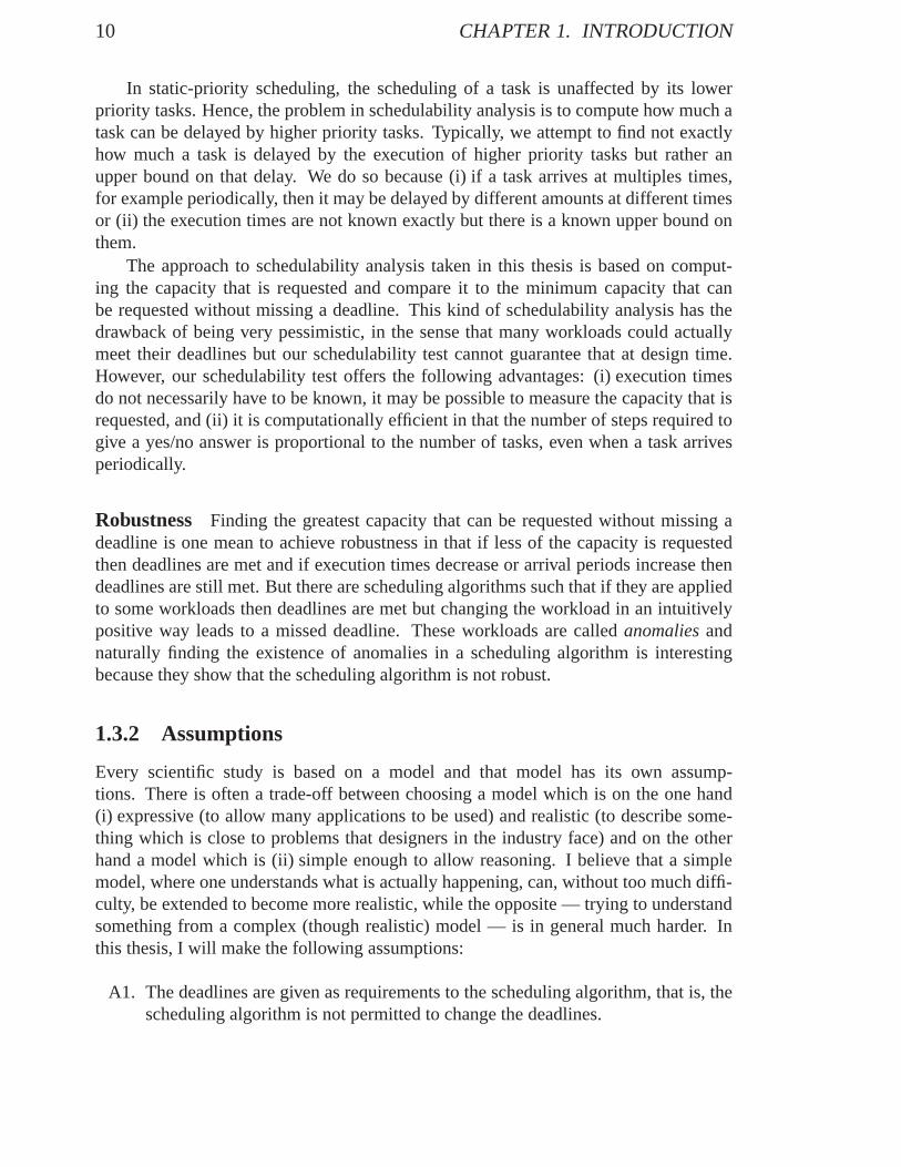
Example 5 Consider the following four periodic tasks:(T1 = 3; C1 = 1); (T2 =3; C2 = 1); (T3 = 3; C3 = 2); (T4 = 4; C4 = 2). If priorities are assigned to thesetasks according to RM (and�3 is given lower priority than both�1 and�2) and the firsttask instances arrive at the same time, the tasks can be scheduled on two processors(see Figure 2.4(a)). However, if we swap the priority order of�2 and�3, task�4 missesa deadline (see Figure 2.4(b)). �
Observation 2 implies that Audsley’s priority-assignment scheme cannot be ex-tended from uniprocessor scheduling to multiprocessor scheduling in a straightforwardmanner.
2.4 Detailed contributions
Recall that the problem addressed in this thesis is:
How much of the capacity of a multiprocessor system can be requestedwithout missing a deadline when static-priority preemptive scheduling isused?
26 CHAPTER 2. INTRODUCTION TO PERIODIC SCHEDULING
0 4 8 12 16
P2 -
P1 -
�4 " " " " "�3 " " " " " "�2 " " " " " "�1 " " " " " "
�1;1 �1;2 �1;3 �1;4 �1;5�3;1 �3;2 �3;3 �3;4 �3;5
�2;1 �2;2 �2;3 �2;4 �2;5�4;1 �4;2 �4;3 �4;3
(a) Task set schedulable
0 4 8 12 16
P2 -
P1 -
�4 " " " " "�3 " " " " " "�2 " " " " " "�1 " " " " " "
�1;1 �1;2 �1;3 �1;4 �1;5�2;1 �2;2 �2;3 �2;4 �2;5
�3;1 �3;2 �3;3 �3;4 �3;5�4;1 �4;2 �4;3 �4;3
(b) Task set unschedulable
Figure 2.4:When the priority order of the higher-priority tasks�2 and�3 are swapped,the first instance of�4 becomes unschedulable (misses its deadlines by two time units).This is because�4 barely meets its deadline and the interference during the first taskperiod increases (from 2 to 3).
My way of measuring capacity is by using the concept of the utilization bound, asdefined earlier in Section 2.2. So, to answer this question, I have:
C1. shown that no global static-priority scheduling algorithm can have a utilizationbound greater than0:5 (see Chapter 3).
C2. designed a global static-priority scheduling algorithm with a utilization bound of1=3 (see Chapter 3). Previously, the only available utilization bound of globalstatic-priority scheduling was0 [DL78]. The idea behind my new algorithm isto separate tasks with a high utilization from tasks with a low utilization and toassign priorities to tasks in these different groups in different ways. The ideaof separating tasks on the basis of utilization has previously been used in parti-tioning algorithms [BLOS95]. This idea has also been used in global schedul-

2.4. DETAILED CONTRIBUTIONS 27
ing [SB02]6 but it differs from my algorithm in that it used job-static priorityscheduling whereas I use task-static priority scheduling.
C3. designed a partitioned static-priority scheduling algorithm with a utilizationbound of1=2 (see Chapter 4). Previously, the greatest utilization bound was0:41 [OB98, LDG01]. The new utilization bound is the best possible (see C1above).
C4. shown that scheduling anomalies can happen in several previously knownpreemptive multiprocessor scheduling algorithms for global and partitionedscheduling (see Chapter 5). I have also designed a partitioned scheduling al-gorithm that is free from anomalies. Previously, anomalies were only knownin non-preemptive scheduling [Gra69] and scheduling with preemption but re-stricted migration [HL94].
6This work was done concurrently with my work.

28 CHAPTER 2. INTRODUCTION TO PERIODIC SCHEDULING

Chapter 3
Global scheduling
3.1 Introduction
In global scheduling, the only way the scheduling algorithm can affect whether tasksmeet their deadlines is to assign priorities. A natural choice is to use RM, but it unfor-tunately has a utilization bound of zero, as illustrated in Example 6.
Example 6 ([Dha77, DL78]) Considerm+ 1 periodic tasks that should be scheduledonm processors using RM. Let tasks�i (where1 � i � m) haveTi = 1,Ci = 2�, andthe task�m+1 haveTm+1 = 1 + �,Cm+1 = 1. All tasks arrive at the same time whenthey arrive for the first time; let us call this timet = 0. Tasks�i (where1 � i � m)will execute immediately when they arrive and complete their execution2� units later.�m+1 then executes from time2� until 1 + �, that is,1 � � time units.�m+1 needs toexecute1 time unit, however, so it misses its deadline. By lettingm ! 1 and� ! 0,we have a task set with a system utilization of zero, but a deadline is still missed.�
Since RM can perform poorly in global scheduling, there is a need for a betterpriority assignment scheme — a priority assignment scheme with a utilization boundthat is greater than zero. This chapter presents the RM-US approach that I invented forglobal scheduling to achieve a utilization bound greater than zero. We will do so bypresenting theRM-US(m/(3m-2)) scheme, the first published algorithm that used theRM-US approach.
Organization of this chapter. The remainder of this chapter is organized as fol-lows. In Section 3.2, we briefly describe two major results that we will be using in theremainder of this chapter. In Section 3.3, we present AlgorithmRM-US(m/(3m-2)),our static-priority multiprocessor algorithm for scheduling arbitrary periodic task sys-tems, and prove that AlgorithmRM-US(m/(3m-2))successfully schedules any periodic
29

30 CHAPTER 3. GLOBAL SCHEDULING
task system with utilization� m2=(3m � 2) onm identical processors. Finally, Sec-tion 3.4 gives an upper bound on the utilization bound of priority-assignment schemesin global scheduling.
3.2 Results we will use
Some very interesting and important results in real-time multiprocessor scheduling the-ory were obtained in the mid 1990’s. We will make use of two of these results in thischapter; these two results are briefly described below.
Resource augmentation. It has previously been shown [BKM+92, BKM+91b,BHS94] that on-line real-time scheduling algorithms tend to perform extremely poorlyunder overloaded conditions. Phillips, Stein, Torng, and Wein [PSTW97] explored theuse ofresource-augmentationtechniques for the on-line scheduling of real-time jobs1;the goal was to determine whether an on-line algorithm, if provided with faster pro-cessors than those available to a clairvoyant algorithm, could perform better than isimplied by the bounds derived in [BKM+92, BKM+91b, BHS94]. Although we arenot studying on-line scheduling in this chapter — all the parameters of all the periodictasks are assumed a priori known — it nevertheless turns out that a particular resultfrom [PSTW97] will prove very useful to us in our study of static-priority multiproces-sor scheduling. We present this result below.
The focus of [PSTW97] was the scheduling of individual jobs, and not periodictasks. Accordingly, let us define ajob Jj = (rj ; ej ; dj) as being characterized by anarrival timerj , an execution requirementej , and a deadlinedj , with the interpretationthat this job needs to execute forej units over the interval[rj ; dj). (Thus, the periodictask�i = (Ci; Ti; Si) generates an infinite sequence of jobs with parameters(Sk + k �Ti; Ci; Sk + (k + 1) � Ti), k = 0; 1; 2; : : : ; in the remainder of this chapter, we willoften use the symbol� itself to denote the infinite set of jobs generated by the tasks inperiodic task system� .)
Let I denote any set of jobs. For any algorithmA and time instantt � 0, letW (A;m; s; I; t) denote the amount of work done by algorithmA on jobs ofI over theinterval [0; t), while executing onm processors of speeds each. Awork-conservingscheduling algorithm is one that never idles a processor while there is some active jobawaiting execution.
Theorem 1 (Phillips et al.) For any set of jobsI, any time-instantt � 0, any work-conserving algorithmA, and any algorithmA0, it is the case that
W (A;m; (2� 1
m) � s; I; t) �W (A0;m; s; I; t): (3.1)
1Resource augmentation as a technique for improving the performance on on-line schedulingalgorithms was formally proposed by Kalyanasundaram and Pruhs [KP95].

3.2. RESULTS WE WILL USE 31
�
That is, anm-processor work-conserving algorithm completes at least as muchexecution as any other algorithm, if provided processors that are(2 � 1=m) times asfast.
Predictable scheduling algorithms. Ha and Liu [HL94] have studied the issue ofpredictability in the multiprocessor scheduling of real-time systems from the followingperspective.
Definition 1 (Predictability) Let A denote a scheduling algorithm, andI =fJ1; J2; : : : ; Jng any set ofn jobs,Jj = (rj ; ej ; dj). Let fj denote the time at whichjob Jj completes execution whenI is scheduled by algorithmA.
Now, consider any setI 0 = fJ 01; J 02; : : : ; J 0ng of n jobs obtained fromI as follows.JobJ 0j has an arrival timerj , an execution requiremente0j � ej , and a deadlinedj (i.e.,job J 0j has the same arrival time and deadline asJj , and an execution requirement nolarger thanJj ’s). Let f 0j denote the time at which jobJj completes execution whenIis scheduled using algorithmA. Scheduling algorithmA is said to bepredictable ifand only if for any set of jobsI and for any suchI 0 obtained fromI, it is the case thatf 0j � fj for all j.
Informally, Definition 1 recognizes the fact that the specified execution-requirement parameters of jobs are typically onlyupper boundson the actual execution-requirements during run-time, rather than the exact values. For a predictable schedulingalgorithm, one may determine an upper bound on the completion-times of jobs by ana-lyzing the situation under the assumption that each job executes for an amount equal tothe upper bound on its execution requirement; it is guaranteed that the actual completiontime of jobs will be no later than this determined value.
Since a periodic task system generates a set of jobs, Definition 1 may be extendedin a straightforward manner to algorithms for scheduling periodic task systems: analgorithm for scheduling periodic task systems is predictable iff for any periodic tasksystems� = f�1; �2; : : : ; �ng it is the case that the completion time of each job whenevery job of�i has an execution requirement exactly equal toCi is an upper bound onthe completion time of that job when every job of�i has an execution requirement ofat mostCi, for all i; 1 � i � n.
Ha and Liu define a scheduling algorithm to bepriority driven 2 if and only if itsatisfies the condition thatfor every pair of jobsJi andJj , if Ji has higher priority thanJj at some instant in time, thenJi alwayshas higher priority thanJj . Notice that anyglobal static-priority algorithm for scheduling periodic tasks satisfies this condition, andis hence priority-driven. However, the converse is not true in that not all algorithms forscheduling periodic tasks that meet the definition of priority-driven are global static-priority algorithms (e.g., notice that the earliest deadline first scheduling algorithm,
2The word “priority-driven” is synonymous to our word “job-static priority”.

32 CHAPTER 3. GLOBAL SCHEDULING
which schedules at each instant the currently active job whose deadline is the smallest,is a priority-driven algorithm, but is not a static-priority algorithm).
The result from the work of Ha and Liu [HL94] that we will be using can be statedas follows.
Theorem 2 (Ha and Liu) Any priority-driven scheduling algorithm is predictable.
3.3 Algorithm RM-US(m/(3m-2))
We now present AlgorithmRM-US(m/(3m-2)), a static-priority global scheduling al-gorithm for scheduling periodic task systems, and derive a utilization-based sufficientschedulability condition for AlgorithmRM-US(m/(3m-2)); in particular, we will provethat any task system� satisfyingU(�) � m2=(3m � 2) will be scheduled to meet alldeadlines onm unit-speed processors by AlgorithmRM-US(m/(3m-2)). This is howwe will proceed. In Section 3.3.1, we will consider a restricted category of periodictask systems, which we call “light” systems; we will prove that the multiprocessorrate-monotonic scheduling algorithm (we will henceforth refer to the multiprocessor rate-monotonic algorithm as AlgorithmRM ), which is a global static-priority algorithm thatassigns tasks priorities in inverse proportion to their periods, will successfully scheduleany light system. Then in Section 3.3.2, we extend the results concerning light systemsto arbitrary systems of periodic tasks. We extend AlgorithmRM to define a globalstatic-priority scheduling algorithm which we call AlgorithmRM-US(m/(3m-2)), andprove that AlgorithmRM-US(m/(3m-2)) successfully schedules any periodic task sys-tem with utilization at mostm2=(3m� 2) onm identical processors.
3.3.1 “Light” systems
Definition 2 A periodic task system� is said to be alight system onm processorsif itsatisfies the following two properties
Property P1: For each�i 2 �; Ui � m
3m� 2
Property P2: U(�) � m2
3m� 2
We will consider the scheduling of task systems satisfying Property P1 and PropertyP2 above, using the rate-monotonic scheduling algorithm (AlgorithmRM ).
Theorem 3 Any periodic task system� that is light onm processors will be scheduledto meet all deadlines onm processors by AlgorithmRM .
Proof: Let us suppose that ties are broken by AlgorithmRM such that�i has greaterpriority than �i+1 for all i, 1 � i < n. Notice that whether jobs of�k meet

3.3. ALGORITHM RM-US(M/(3M-2)) 33
their deadlines under AlgorithmRM depends only upon the jobs generated by thetasksf�1; �2; : : : ; �kg, and are completely unaffected by the presence of the tasks�k+1; : : : ; �n. Fork = 1; 2; : : : ; n, let us define the task-set� (k) as follows:
� (k)def= f�1; �2; : : : ; �kg:
Our proof strategy is as follows. We will prove that AlgorithmRM will schedule� (k)
in such a manner that all jobs of the lowest-priority task�k complete by their deadlines.Our claim that AlgorithmRM successfully schedules� would then follow by inductiononk.
Lemma 3.1 Task system� (k) is feasible onm processors each of computing capacity( m2m�1 ).
Proof: Sincem � 2, notice that3m� 2 > 2m� 1. SinceUi � m3m�2 for each task�i
(by Property P1 above), it follows that
Ui � m
2m� 1(3.2)
Similarly fromU(�) � m2
3m�2 (Property P2 above) and� (k) � � , it can be derived that
X�i2�(k)
Ui � m2
2m� 1: (3.3)
As a consequence of Inequalities 3.2 and 3.3 we may conclude that� (k) can bescheduled to meet all deadlines onm processors each of computing capacity( m
2m�1 ):the processor-sharing schedule (which we will henceforth denoteOPT), which assignsa fractionUi of a processor to�i at each time-instant bears witness to the feasibility of� (k).End proof (of Lemma 3.1)
Since m2m�1 � (2 � 1
m ) = 1, it follows from Theorem 1, the existence of thescheduleOPT described in the proof of Lemma 3.1, and the fact that AlgorithmRM iswork-conserving, that
W (RM ;m; 1; � (k); t) �W (OPT;m;m
2m� 1; � (k); t) (3.4)
for all t � 0; i.e., at any time-instantt, the amount of work done on� (k) by Algo-rithm RM executing onm unit-speed processors is at least as much as the amount ofwork done on� (k) by OPT onm m
2m�1 -speed processors.
Lemma 3.2 All jobs of �k meet their deadlines when� (k) is scheduled using Algo-rithm RM .

34 CHAPTER 3. GLOBAL SCHEDULING
Proof: Let us assume that the first(` � 1) jobs of �k have met their deadlines underAlgorithm RM ; we will prove below that the’th job of �k also meets its deadline. Thecorrectness of Lemma 3.2 will then follow by induction on`, starting with` = 1.
The `’th job of �k arrives at time-instantSk + (` � 1)Tk, has a deadline at time-instantSk+ `Tk, and needsCk units of execution. From Inequality 3.4 and the fact thatthe processor-sharing scheduleOPT schedules each task�j for Uj � max(0; Sk + (` �1)Tk � Sj) units over the interval[0; Sk + (`� 1)Tk), we have
W (RM ;m; 1; � (k); Sk + (`� 1)Tk) �kX
j=1
(Uj �max(0; Sk + (`� 1)Tk � Sj)) (3.5)
Also, at leastPk�1
j=1 (Uj �max(0; Sk + (`� 1)Tk � Sj)) units of this execution by Al-gorithm RM was of tasks�1; �2; : : : ; �k�1 — this follows from the fact that exactly(` � 1)TkUk units of �k’s work has been generated prior to instantSk + (` � 1)Tk;the remainder of the work executed by AlgorithmRM must therefore be generated by�1; �2; : : : ; �k�1.
The cumulative execution requirement of all the jobs generated by the tasks�1; �2; : : : ; �k�1 that arrive prior to the deadline of�k’s `’th job is bounded from aboveby
k�1Xj=1
lmax(0; Sk + `Tk � Sj)
Tj
mCj
<k�1Xj=1
max(0; Sk + `Tk � Sj)
TjCj + Cj (3.6)
As we have seen above (the discussion following Inequality 3.5) at leastPk�1j=1 (Uj �max(0; Sk + (`� 1)Tk � Sj)) of this gets done prior to time-instantSk+
(`� 1)Tk; hence, at most
k�1Xj=1
�Uj �
�max(0; Sk + `Tk � Sj)� (3.7)
max(0; Sk + (`� 1)Tk � Sj)��
+k�1Xj=1
Cj
remains to be executedafter time-instantSk + (` � 1)Tk. We will now show thatmax(0; Sk + `Tk � Sj) � max(0; Sk + (` � 1)Tk � Sj) � Tk by considering thefollowing cases:
I . Sk + (`� 1)Tk � Sj < 0
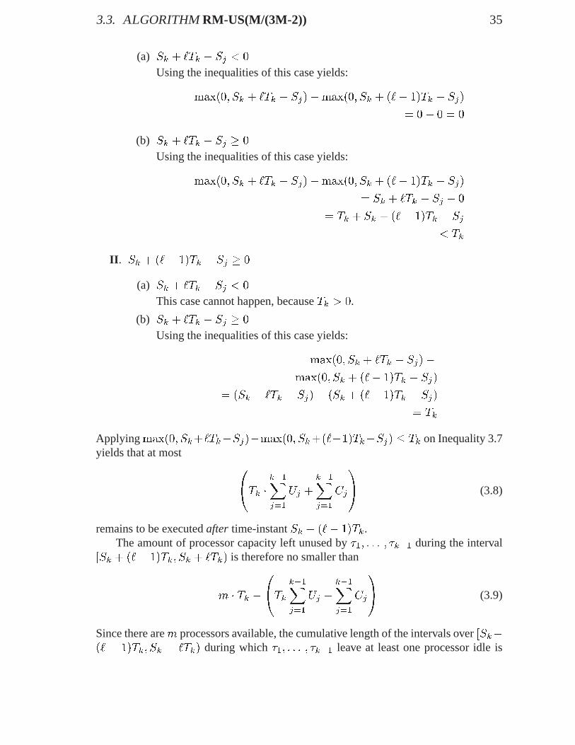
3.3. ALGORITHM RM-US(M/(3M-2)) 35
(a) Sk + `Tk � Sj < 0
Using the inequalities of this case yields:
max(0; Sk + `Tk � Sj)�max(0; Sk + (`� 1)Tk � Sj)
= 0� 0 = 0
(b) Sk + `Tk � Sj � 0
Using the inequalities of this case yields:
max(0; Sk + `Tk � Sj)�max(0; Sk + (`� 1)Tk � Sj)
= Sk + `Tk � Sj � 0
= Tk + Sk + (`� 1)Tk � Sj
< Tk
II . Sk + (`� 1)Tk � Sj � 0
(a) Sk + `Tk � Sj < 0
This case cannot happen, becauseTk > 0.
(b) Sk + `Tk � Sj � 0
Using the inequalities of this case yields:
max(0; Sk + `Tk � Sj)�max(0; Sk + (`� 1)Tk � Sj)
= (Sk + `Tk � Sj)� (Sk + (`� 1)Tk � Sj)
= Tk
Applyingmax(0; Sk+`Tk�Sj)�max(0; Sk+(`�1)Tk�Sj) � Tk on Inequality 3.7yields that at most
0@Tk �
k�1Xj=1
Uj +k�1Xj=1
Cj
1A (3.8)
remains to be executedafter time-instantSk + (`� 1)Tk.The amount of processor capacity left unused by�1; : : : ; �k�1 during the interval
[Sk + (`� 1)Tk; Sk + `Tk) is therefore no smaller than
m � Tk �0@Tk
k�1Xj=1
Uj +k�1Xj=1
Cj
1A (3.9)
Since there arem processors available, the cumulative length of the intervals over[Sk+(` � 1)Tk; Sk + `Tk) during which�1; : : : ; �k�1 leave at least one processor idle is

36 CHAPTER 3. GLOBAL SCHEDULING
minimized if the different processors tend to idle simultaneously (in parallel); hence, alower bound on this cumulative length of the intervals over[Sk + (`� 1)Tk; Sk + `Tk)during which�1; : : : ; �k�1 leave at least one processor idle is given by(m � Tk ��TkPk�1
j=1 Uj +Pk�1
j=1 Cj
�)=m, which equals
Tk � 1
m
0@Tk
k�1Xj=1
Uj +k�1Xj=1
Cj
1A (3.10)
For the`’th job of �k to meet its deadline, it suffices that this cumulative interval lengthbe at least as large at�k’s execution requirement; i.e.,
Tk � 1
m(Tk
k�1Xj=1
Uj +k�1Xj=1
Cj) � Ck
� Ck
Tk+
1
m(k�1Xj=1
Uj +k�1Xj=1
Cj
Tk) � 1
( (SinceTk � Tj for j < k)
Uk +1
m(2
k�1Xj=1
Uj) � 1 (3.11)
Let us now simplify the lhs of Inequality 3.11 above:
Uk +1
m(2
k�1Xj=1
Uj)
� Uk +1
m(2
kXj=1
Uj � 2Uk)
� (By Property P2 of task system� )
Uk(1� 2
m) +
2m
3m� 2� (By Property P1 of task system� )
m
3m� 2(1� 2
m) +
2m
3m� 2(3.12)
= 1 (3.13)
From Inequalities 3.11 and 3.13, we may conclude that the`’th job of �k does meet itsdeadline.End proof (of Lemma 3.2)
The correctness of Theorem 3 follows from Lemma 3.2 by induction onk, withk = m being the base case (that�1; �2; : : : �m meet all their deadlines directly followsfrom the fact that there arem processors available in the system).

3.3. ALGORITHM RM-US(M/(3M-2)) 37
End proof (of Theorem 3)
3.3.2 Arbitrary systems
In Section 3.3.1, we saw that AlgorithmRM successfully schedules any periodic tasksystem� with utilizationU(�) � m2=(3m � 1) onm identical processors,providedeach�i 2 � has a utilizationUi � m=(3m � 2). We now relax the restriction onthe utilization of each individual task; rather, we permit anyUi � 1 for each�i 2 � .That is, we will consider in this section the static-priority global scheduling of any tasksystem� satisfying the condition
U(�) � m2
3m� 2:
For such task systems, we define the static priority-assignment scheme Algo-rithm RM-US(m/(3m-2)) as follows.
Algorithm RM-US(m/(3m-2)) assigns (static) priorities to tasks in� according tothe following rule:
if Ui > m3m�2 then �i has the highest priority (ties broken arbitrarily)
if Ui � m3m�2 then �i has rate-monotonic priority.
Example 1 As an example of the priorities assigned by AlgorithmRM-US(m/(3m-2)),consider a task system
�def= f�1 = (T1 = 7; C1 = 1); �2 = (T2 = 10; C2 = 2); �3 = (T3 = 20; C3 = 9);
�4 = (T4 = 22; C4 = 11); �5 = (T5 = 25; C5 = 2)g
to be scheduled on a platform of3 identical unit-speed processors. The utilizationsof these five tasks are� 0:143, 0:2, 0:45, 0:5, and0:08 respectively. Form = 3,m=(3m � 2) equals3=7 � 0:4286; hence, tasks�3 and�4 will be assigned highestpriorities, and the remaining three tasks will be assigned rate-monotonic priorities. Thepossible priority assignments are therefore as follows (highest-priority task listed first):
�3; �4; �1; �2; �5
or
�4; �3; �1; �2; �5
�

38 CHAPTER 3. GLOBAL SCHEDULING
Theorem 4 Any periodic task system� with utilization U(�) � m2=(3m � 2)will be scheduled to meet all deadlines onm unit-speed processors by Algo-rithm RM-US(m/(3m-2)).
Proof: Assume that the tasks in� are indexed according to the priorities assigned tothem by AlgorithmRM-US(m/(3m-2)). First, observe that sinceU(�) � m2=(3m�2),while each task�i that is assigned highest priority hasUi strictly greater thanm=(3m�2), there can be at most(m � 1) such tasks that are assigned highest priority. Letkodenote the number of tasks that are assigned the highest priority; i.e.,�1; �2; : : : ; �koeach have utilization greater thanm=(3m� 2), and�ko+1; : : : �n are assigned priorities
rate-monotonically. Letmodef= m� ko.
Let us first analyze the task system� , consisting of the tasks in� each havingutilization� m=(3m� 2):
�def= � n � (ko) :
The utilization of� can be bounded from above as follows:
U(�) = U(�)� U(� (ko))
<m2
3m� 2� ko � m
3m� 2
=m(m� ko)
3m� 2
� (m� ko) � (m� ko)
3(m� ko)� 2
=m2o
3mo � 2(3.14)
Furthermore, for each�i 2 � , we have
Ui � m
3m� 2� mo
3mo � 2: (3.15)
From Inequalities 3.14 and 3.15, we conclude that� is a periodic task system that islight onmo processors. Hence by Theorem 3,� can be scheduled by AlgorithmRM tomeet all deadlines onmo processors.
Now, consider the task system~� obtained from� by replacing each task�i 2 � thathas a utilizationUi greater thanm=(3m � 2) by a task with the same period, but withutilization equal to one:
~�def= �
[�[(Ci;Ti;Si)2�(ko)f(Ti; Ti; Si)g�:
Notice that AlgorithmRM-US(m/(3m-2)) will assign identical priorities to corre-sponding tasks in� and� (where the notion of “corresponding” is defined in the obvious

3.4. BOUND ON UTILIZATION BOUNDS 39
manner). Also notice that when scheduling~� , Algorithm RM-US(m/(3m-2)) will de-vote ko processors exclusively to theko tasks in� (ko) (these are the highest-prioritytasks, and each have a utilization equal to unity) and will be executing AlgorithmRMon the remaining tasks (the tasks in� ) upon the remainingmo = (m� ko) processors.As we have seen above, AlgorithmRM schedules the tasks in� to meet all deadlines;hence, AlgorithmRM-US(m/(3m-2)) schedules~� to meet all deadlines of all jobs.
Finally, notice that an execution of AlgorithmRM-US(m/(3m-2)) on task system� can be considered to be an instantiation of a run of AlgorithmRM-US(m/(3m-2))on task system~� , in which some jobs — the ones generated by tasks in� (ko) —do not execute to their full execution requirement. By the result of Ha and Liu(Theorem 2), it follows that AlgorithmRM-US(m/(3m-2)) is a predictableschedul-ing algorithm, and hence each job of each task during the execution of Algo-rithm RM-US(m/(3m-2)) on task system� completes no later than the correspondingjob during the execution of AlgorithmRM-US(m/(3m-2)) on task system~� . And,we have already seen above that no deadlines are missed during the execution ofAlgorithm RM-US(m/(3m-2)) on task system~� .End proof (of Theorem 4)
3.4 Bound on utilization bounds
We can show an upper bound on the best possible system utilization bound for anystatic-priority multiprocessor scheduling algorithm. Consider the task set
�def= f�1 = (L; 2L� 1); �2 = (L; 2L� 1); : : : ;
�m = (L; 2L� 1); �m+1 = (L; 2L� 1)gto be scheduled onm processors (L is a positive integer) when all tasks arrive at time0. For this task set, the system utilization isL=(2L � 1) + (L=(2L � 1))=m. Forglobal static-priority scheduling, deadlines will be missed for this task set because allm highest priority tasks will execute at the same time and occupyL time units during[0,2L � 1). There will beL � 1 time units available for a lower priority tasks, but thelowest priority task needsL time units and thus misses its deadline. By lettingL!1andm!1, the task set is unschedulable at a system utilization of1=2. Consequently,the utilization guarantee bound for any global static-priority multiprocessor schedulingalgorithm cannot be higher than 1/2 of the capacity of the multiprocessor platform.
This bound of0:5 applies to all global static-priority algorithms; it applies evento very complex algorithms such as algorithms that enumerate all possible orders ofpriorities of tasks. However, if we consider simpler algorithms, algorithms (such asRM-US(m/(3m-2))) that assign a priority to a task based on only information of thattask — not other tasks, then the utilization bound that we can achieve is even lower.This is illustrated by Theorem 3.1.

40 CHAPTER 3. GLOBAL SCHEDULING
Theorem 3.1 If the priorities of global traditional static-priority scheduling are as-signed according to the functionprio(�i) = f(Ti; Ci) and if the functionf(Ti; Ci) isscale invariant, that isf(Ti; Ci) < f(Tj ; Cj), f(A�Ti; A�Ci) < f(A�Tj ; A�Cj)8A > 0, then the utilization bound is no greater than
p2� 1.
Proof The proof is based on contradiction. Let us assume that there was one functionf(Ti; Ci) which had a utilization bound greater than
p2� 1. For the case ofm!1,
it is necessary that:
f(T = 1; C =p2� 1 + �) < f(T =
p2; C = 2�
p2) (3.16)
otherwise, a task set withm tasks ofTi = 1,Ci =p2 � 1 + � and one task with
Tm+1 =p2, Cm+1 = 2 � p
2 with all tasks arriving at the same time would miss adeadline because them tasks would receive the highest priority and hence this wouldcontradict the utilization bound of
p2� 1.
f(Ti; Ci) is scale invariant. We can divide each task parameter byp2. Hence we
have:
f(T =1p2; C = 1� 1p
2+
�p2) < f(T = 1; C =
p2� 1) (3.17)
Considerm+1 tasks to be scheduled on m processors. The tasks are characterizedas: (Ti = 1,Ci =
p2�1) for i=1..m and (Tm+1 = 1=
p2,Cm+1 = 1�1=
p2+ �=
p2).
All tasks arrive at time0. Because of Equation 3.17, we have that�1; �2; :::�m receivethe highest priority and hence they execute during [0,
p2� 1). During [
p2� 1,1=
p2),
there are1 � (1=p2) time units available for the lower priority task�m+1 to execute.
During another time interval [0,1=p2), there are still1�(1=
p2) time units available for
the lower priority task�m+1 to execute. But�m+1 needs to execute1� 1=p2 + �=
p2
time units and hence it needs to execute�=p2 time units more. Hence it misses its
deadline. The system utilization isp2� 1 whenm!1. That is a contradiction.�
We can conclude that although our algorithmRM-US(m/(3m-2)) only achieved autilization bound of0:33, it is not too far from what can be achieved given that it onlytakes a limited amount of information into account in its decisions.

Chapter 4
Partitioned scheduling
4.1 Introduction
Before I started my research, the partitioned method was well explored [Dha77, DL78,DD85, DD86, BLOS95, OS95a, OS95b, LMM98b, SVC98, LW82, OB98] and it wasknown that no partitioned scheduling algorithm can have a utilization bound greaterthan 0.50 but the best utilization bound known so far was 41% [OB98, LDG01], leavingroom for improvements.
In this chapter, we show that an algorithm, called R-BOUND-MP-NFR, has a uti-lization bound of 50%. We hence close the problem.
The remainder of this chapter is organized as follows. Section 4.2 gives a back-ground on partitioned scheduling. We propose an algorithm and prove its utilizationbound, first in Section 4.3 where the periods of tasks are restricted and later in Sec-tion 4.4 where the periods of tasks are not restricted.
4.2 Background on partitioned scheduling
Recall that the partitioned method divides tasks into partitions, each having its owndedicated processor. Unfortunately, the problem of deciding whether a schedulablepartition exists is NP-complete [LW82]. Therefore many heuristics for partitioninghave been proposed, a majority of which are versions of the bin-packing algorithm1.These bin-packing algorithms rely on a schedulability test in order to know whether atask can be assigned to a processor or not. This reduces our problem from partitioning
1The bin-packing algorithm works as follows: (1) sort the tasks according to some criterion;(2) select the first task and an arbitrary processor; (3) attempt to assign the selected task to theselected processor by applying a schedulability test for the processor; (4) if the schedulability testfails, select the next available processor; if it succeeds, select the next task; (5) goto step 3.
41

42 CHAPTER 4. PARTITIONED SCHEDULING
a set of tasks to meet deadlines into the problem of partitioning a set of tasks such that,on every processor, the schedulability test can guarantee that all tasks on that processormeet their deadlines. As a schedulability test, a natural choice is to use the knowledgethat: if
Pnpi=1 Ci=Ti � np � (21=np �1) and rate-monotonic is used to schedule tasks on
processorp then all deadlines are met. (We letnp denote the number of tasks assignedto processorp.) This schedulability test is often used, but as shown in Example 7below, this bound is not tight enough to allow us to design a multiprocessor schedulingalgorithm with a utilization bound of 50%.
Example 7 Considerm + 1 tasks withTi = 1 andCi =p2 � 1 + � to be scheduled
onm processors. For this system, there must be a processorp which is assigned twotasks. On that processor the utilization is
Pnpi=1 Ci=Ti = 2 � (p2 � 1 + �) which is
greater than2 � (p2� 1). Hence, there is no way to partition tasks so that all tasks canbe guaranteed by this schedulability test to meet deadlines. We can do this reasoningfor everym and every�. By letting� ! 0 andm ! 1 we can see that the utilizationbound for algorithms that are based on this schedulability test cannot be greater thanp2� 1, which is approximately 41%. �
Note that the task set in Example 7 could actually be guaranteed by a necessaryand sufficient schedulability test to meet deadlines (provided that� is not too large).It is known that if all tasks are harmonic2 then the uniprocessor utilization bound is100%3, and then the task set in Example 7 could be assigned with two tasks on oneprocessor. A uniprocessor schedulability test that could exploit this information couldallow a multiprocessor scheduling algorithm to achieve a utilization bound of 50%.This is what we will do in the following.
R-BOUND [LMM98b] is a uniprocessor schedulability test which exploits har-monicity. Letrp denote the fraction between the maximum and the minimum periodamong the tasks assigned to processorp. If we restrict our attention to the case in which8p : 1 � rp < 2 (we will relax this restriction later), we have the following theorem.
Theorem 4.1 (Lauzac, Melhem and Mosse[LMM98b]) Let B(rp; np) =
np(r1=npp � 1) + 2=rp � 1. If
Pnpi=1 Ci=Ti � B(rp; np) and rate-monotonic is
used to schedule tasks on processorp then all deadlines are met.
R-BOUND-MP is a previously known multiprocessor scheduling algorithm thatexploits R-BOUND [LMM98b]. R-BOUND-MP combined R-BOUND with a first-fitbin-packing algorithm. To show which utilization bound a partitioned scheduling algo-rithm can achieve, we will design two derivatives of R-BOUND-MP. First, we will con-sider an algorithm R-BOUND-MP-NFRNS (R-BOUND-MP with next-fit-ring noscal-
2In a harmonic task set, the periodsTi andTj of any two tasks�i and�j are related as follows:eitherTi is an integer multiple ofTj , orTj is an integer multiple ofTi.
3This is easy to see by dropping the ceiling in the equations/inequalities in exact schedulabilitytests [JP86, LSD89].

4.3. RESTRICTED PERIODS 43
ing) and prove its utilization bound when1 � max�i2� Timin�i2� Ti
< 2. ( � denotes the set of alln tasks.) Then we will consider the algorithm R-BOUND-MP-NFR (R-BOUND-MPwith next-fit-ring) and prove its utilization bound when periods are not restricted.
4.3 Restricted periods
In this section, we assume that1 � max�i2� Timin�i2� Ti
< 2 holds. Clearly it means that
no matter how we assign tasks to processors, it holds that8p : 1 � rp < 2 andhence Theorem 4.1 can be used. We will use the algorithm R-BOUND-MP-NFRNS. Itworks as follows: (i) sort tasks in ascending order of periods, that is, the task with theshortest period is considered first, (ii) use Theorem 4.1 as a schedulability test on eachuniprocessor, (iii) assign tasks with the next-fit bin-packing algorithm and (iv) when atask cannot be assigned to processor m, try to assign it to processor 1, if this does notwork then declare FAILURE. If the algorithm terminates and has partitioned the wholetask set then the algorithm declares SUCCESS.
Example 8 illustrates the workings of our algorithm R-BOUND-MP-NFRNS.
Example 8 Consider4 tasks withf(T1 = 1:1; C1 = 0:935); (T2 = 1:3; C2 =0:26); (T3 = 1:2; C3 = 0:084); (T4 = 1; C4 = 0:1)g to be scheduled on2 processorsusing R-BOUND-MP-NFRNS. The algorithm sorts the tasks in ascending order of peri-ods. Reordering the tasks yields:f(T4 = 1; C4 = 0:1); (T1 = 1:1; C1 = 0:935); (T3 =1:2; C3 = 0:084); (T2 = 1:3; C2 = 0:26)g. We can compute the utilizations of tasks:u4 = 0:1,u1 = 0:85,u3 = 0:07 andu2 = 0:2.
The current processor is processor1. Tasks are now assigned in order.�4 is as-signed to processor 1. Then an attempt is made to assign�1 to processor 1, but it failsbecause theT1=T4 = 1:1, andn1 = 2 gives a utilization bound of0:915 for these twotasks, and the sum of utilization of these two tasks is 0.95. Hence�1 is assigned toprocessor 2.
Now, processor 2 is the current processor. An attempt is made to assign�3 proces-sor 2, and it succeeds becauseT3=T1 = 1:2=1:1 = 1:09, andn2 = 2 gives a utilizationbound of0:922 for these two tasks, and the sum of utilization of these two tasks is0:92.
Processor 2 is still the current processor. An attempt is made to assign�2 to pro-cessor 2, but it fails becausemax(T1; T3; T2)=min(T1; T3; T2) = 1:3=1:1 = 1:18 andn2 = 3 gives a utilization bound of0:86 for these three tasks, and the sum of utilizationof these three tasks is1:12. Since processor 2 is the last processor and�2 failed, wemake an attempt to assign�2 to the first processor, that is, processor 1. This succeedsbecauseT2=T4 = 1:3=1 = 1:3 andn1 = 2 gives a utilization bound of0:818 for thesetwo tasks, and the sum of utilization of these two tasks is0:3. Hence�2 is assigned toprocessor 1. �

44 CHAPTER 4. PARTITIONED SCHEDULING
Theorem 4.2 (Utilization bound of R-BOUND-MP-NFRNS) If R-BOUND-MP-NFRNS is used andT1 � T2 � : : : � Tn andTn=T1 < 2 and 1
m
Pni=1 ui � 1=2, then
R-BOUND-MP-NFRNS will find a partitioning (declare SUCCESS).
Proof Let us assume that the theorem was wrong. Then there must exist a task setthat caused R-BOUND-MP-NFRS to declare failure. If it was not the last task (theone with the longest period) that failed, then we can always remove the task that had ahigher index than the failed task, and then the utilization would be lower. Hence, wecan assume that it was the task with the greatest index that failed. Let�failed denotethat task.
We will now consider the situation when R-BOUND-MP-NFRS failed and use thefollowing notation. Let�pjk be the task that is thekth task assigned to processorj.Let �1 denoteTp21=Tp11. Let�2 denoteTp31=Tp21. : : : Let �m denoteTfailed=Tpm1.Let nj denote the number of tasks that are assigned to processorj. n1 requires furtherexplanation because we assign tasks to processor 1 in two states: first when no processorhas been assigned a task, and later when all processors have been assigned a task. Weletn10 denote the number of tasks assigned to processor1 when R-BOUND-MP-NFRSdeclared failure.n1 denotes the number of tasks assigned to processor1 when�p21 wasassigned to processor2.
Task�p21 could not be assigned to processor 1 because the schedulability test inTheorem 4.1 failed. Hence, on processor 1 it holds that:
up11 + (
n1Xk=2
up1k) + up21 > (n1 + 1)(�1
n1+1
1 � 1) +2
�1� 1 (4.1)
In the same way, on processor 2, it holds that:
up21 + (
n2Xk=2
up2k) + up31 > (n2 + 1)(�1
n2+1
2 � 1) +2
�2� 1 (4.2)
And so on, until processor m, where it holds that:
upm1 + (
nmXk=2
upmk) + ufailed >
(nm + 1)(�1
nm+1m � 1) +
2
�m� 1 (4.3)
Our algorithm R-BOUND-MP-NFRS attempts to assign�failed to processor 1. Itfails so the schedulability test must have failed. Here we do not know anything aboutthe relationships between the periods (other than1 � Tfailed
Ti< 2). Hence we have
up11 + (
n1Xk=2
up1k) + ufailed > (n10+ 1) � (2 1n10+1 � 1) (4.4)
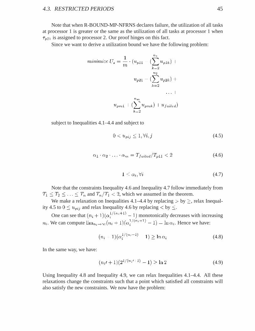
4.3. RESTRICTED PERIODS 45
Note that when R-BOUND-MP-NFRNS declares failure, the utilization of all tasksat processor 1 is greater or the same as the utilization of all tasks at processor 1 when�p21 is assigned to processor 2. Our proof hinges on this fact.
Since we want to derive a utilization bound we have the following problem:
minimize Us =1
m� (up11 + (
n1Xk=2
up1k) +
up21 + (
n2Xk=2
up2k) +
: : :+
upm1 + (
nmXk=2
upmk) + ufailed)
subject to Inequalities 4.1–4.4 and subject to
0 < upij � 1; 8i; j (4.5)
�1 � �2 � : : : � �m = Tfailed=Tp11 < 2 (4.6)
1 � �i; 8i (4.7)
Note that the constraints Inequality 4.6 and Inequality 4.7 follow immediately fromT1 � T2 � : : : � Tn andTn=T1 < 2, which we assumed in the theorem.
We make a relaxation on Inequalities 4.1–4.4 by replacing> by�, relax Inequal-ity 4.5 to0 � upij and relax Inequality 4.6 by replacing< by�.
One can see that(ni + 1)(�1=(ni+1)i � 1) monotonically decreases with increasing
ni. We can computelimni!1(ni + 1)(�1=(ni+1)i � 1) = ln�i. Hence we have:
(ni + 1)(�1=(ni+1)i � 1) � ln�i (4.8)
In the same way, we have:
(ni0+ 1)(21=(ni0+1) � 1) � ln 2 (4.9)
Using Inequality 4.8 and Inequality 4.9, we can relax Inequalities 4.1–4.4. All theserelaxations change the constraints such that a point which satisfied all constraints willalso satisfy the new constraints. We now have the problem:

46 CHAPTER 4. PARTITIONED SCHEDULING
minimize Us =1
m� (up11 + (
n1Xk=2
up1k) +
up21 + (
n2Xk=2
up2k) +
: : :+
upm1 + (
nmXk=2
upmk) + ufailed)
subject to:
up11 + (
n1Xk=2
up1k) + up21 � ln�1 + 2=�1 � 1 (4.10)
up21 + (
n2Xk=2
up2k) + up31 � ln�2 + 2=�2 � 1 (4.11)
: : :
upm1 + (
nmXk=2
upmk) + ufailed � ln�m + 2=�m � 1 (4.12)
up11 + (
n1Xk=2
up1k) + ufailed � ln 2 (4.13)
0 � upij ; 8i; j (4.14)
�1 � �2 � : : : � �m � 2 (4.15)
1 � �i; 8i (4.16)
Note that we are not interested in finding every global minimizer. We simply wantto find a global minimizer. Hence, at a minimizer, we could always move to a new

4.3. RESTRICTED PERIODS 47
point (with primed variables) which satisfies all constraints and does not increase theobjective function in the following way:
upi10 = upi1 +
niXk=2
upik (4.17)
upik0 = 0; 8k � 2 (4.18)
Note thatupij is permitted to be greater than1.If �1 ��2 �: : :��m < 2 then we can increase any�i so that�1 ��2 �: : :��m = 2. This
clearly does not affect the objective function. Neither does it violate any constraintsbecause@(ln�i+2=�i�1)
@�ican be computed to1
�2i� (�i � 2) and this is non-positive
because�i � 2. �i � 2 follows from�1 � �2 � : : : � �m = 2 and1 � �i. Hence wehave the problem:
minimize Us =1
m� (up11 + up21 + : : :+ upm1 + ufailed)
subject to:
up11 + up21 � ln�1 + 2=�1 � 1 (4.19)
up21 + up31 � ln�2 + 2=�2 � 1 (4.20)
: : :
upm1 + ufailed � ln�m + 2=�m � 1 (4.21)
up11 + ufailed > ln 2 (4.22)
0 � upij ; 8i; j (4.23)
�1 � �2 � : : : � �m = 2 (4.24)
1 � �i; 8i (4.25)
Note that in Inequalities 4.19–4.22, each variableupik andufailed show up in ex-actly two constraints. Summing the left-hand side of Inequalities 4.19–4.22 and divid-ing by two gives us a lower bound on the objective function. We can also relax theproblem by dropping Equation 4.23 and Equation 4.25. Hence we have the problem:

48 CHAPTER 4. PARTITIONED SCHEDULING
minimize Us =1
2m� (ln 2 + ln�1 + 2=�1 � 1
+ ln�2 + 2=�2 � 1 + : : :+ ln�m + 2=�m � 1)
subject to:
�1 � �2 � : : : � �m = 2 (4.26)
A necessary condition for a local minimizer is that the gradient of the Lagrangianfunction is zero (see for example Theorem 14.1 in [NS96]). Let� denote the Lagrangemultiplier for �1 � �2 � : : : � �m = 2. Using this gives us that a necessary condition fora local minimizer is:
1
m� (1
2� (1=�1 � 2=�21))� � � �2 � �3 � �4 � : : : � �m = 0
1
m� (1
2� (1=�2 � 2=�22))� � � �1 � �3 � �4 � : : : � �m = 0
1
m� (1
2� (1=�3 � 2=�23))� � � �1 � �2 � �4 � : : : � �m = 0
: : :
1
m� (1
2� (1=�m � 2=�2m))� � � �1 � �2 � �3 � �4 � : : : = 0
Since a global minimizer is a local minimizer, the conditions are also necessary fora global minimizer.
Rewriting each of them and using�1 � �2 � : : : � �m = 2 yields:
1
m� (1� 2=�1) = 4�
1
m� (1� 2=�2) = 4�
: : :

4.4. NOT RESTRICTED PERIODS 49
Algorithm 1 Scale Task Set.Input : A task set� . Output : Another task set� 0.
1: q =T12: for each i 2 �3: q = max(q; Ti)4: end for5: for each i 2 �6: Ti0 = Ti � 2log2(q=Ti)7: Ci0 = Ci � 2log2(q=Ti)8: end for9: sort tasks in� 0 in increasing period
10: return� 0
1
m� (1� 2=�m) = 4�
This implies that:
�1 = �2 = : : : = �m
We now have the following problem:
minimize Us =1
2m� (ln 2 +m � (ln�1 + 2=�1 � 1))
subject to�m1 = 2.Rewriting yields:
minimize Us =ln 2
2m+
1
2� (ln (21=m) +
2
21=m� 1)
We compute@Us@m < 0 andlimm!1 Us = 1=2. Hence we have thatUs � 1=2.This states the theorem. �
4.4 Not restricted periods
In this section, we will see that if task periods are not restricted as they were inthe previous section, Section 4.3, then it is possible to scale the periods and executiontimes of all tasks such that the restriction holds. This is meaningful because we will usea theorem which claims that, if the scaled task set meets all deadlines, then the task setwhich is not scaled also meets its deadlines.

50 CHAPTER 4. PARTITIONED SCHEDULING
Consider two task sets,� and� 0. � is not restricted.� 0 is computed from� accord-ing to Algorithm 1. Note that Algorithm 1 does not change the utilization of tasks. Inaddition we know that:
Theorem 4.3 (Lauzac, Melhem and Mosse[LMM98b]) Given a task set� , let � 0 bethe task set resulting from the application of the algorithm Scale Task Set to� . If � 0 isschedulable on one processor using rate-monotonic scheduling, then� is schedulableon one processor with rate-monotonic scheduling.
Now let R-BOUND-MP-NFR (R-BOUND-MP with next-fit-ring) be an algorithmwhich works as follows. First, each task in� is transformed according to Algorithm 1into � 0 and the tasks in� 0 are then assigned according to R-BOUND-MP-NFRNS. Wecan see that every task in� has a corresponding task in� 0, so �i is assigned to theprocessor where�i0 is.
We are now ready to state our utilization bound of R-BOUND-MP-NFR when tasksare not restricted.
Theorem 4.4 (Utilization bound of R-BOUND-MP-NFR) If R-BOUND-MP-NFR isused and
Pni=1 ui � m=2, then R-BOUND-MP-NFR will find a partitioning (declare
SUCCESS).
Proof The proof is by contradiction. Suppose that the theorem was false. Then therewould exist a task set� with
Pni=1 ui � m=2 which failed. The first thing that R-
BOUND-MP-NFR does is to scale4 the task set, so a scaled task set� 0 will also declarefailure when scheduled by R-BOUND-MP-NFRNS. Sinceui of a task does not changewhen it is scaled, we have that� 0 (which failed) has
Pni=1 ui � m=2. But this is
impossible according to Theorem 4.2. �
4This does not changeui.

Chapter 5
Anomalies
5.1 Introduction
Analysis techniques for real-time systems often require exact knowledge of task char-acteristics, but this is usually not available, for example: the execution time of a taskdepends on input data (which is unknown) or the arrival time of a task depends on whenan external event occurs (which is unknown). Fortunately, upper and lower bounds areoften known, so in order to give guarantees that deadlines are met, an often-used ap-proach is to make assumptions. For example: (i) assume that a task meets its deadlineif it did so when all tasks executed at their maximum execution time or (ii) assume thata task meets its deadline if it did so when all tasks arrived at their maximum arrival fre-quency. Situations where these assumptions do not hold are referred to as schedulinganomalies, and their existence jeopardizes timeliness or complicates the design process.
Anomalies neither occur in popular preemptive uniprocessor scheduling algo-rithms, such as rate-monotonic (RM) and earliest-deadline-first (EDF) [LL73, Mok00],nor in multiprocessor systems with the partitioned scheduling and each processor us-ing an anomaly-free uniprocessor scheduling algorithm. Anomalies can occur in bothuniprocessor and multiprocessor systems [GL89, Mok00, SRS95, LS99, Gra69, HL94]due to non-preemptive scheduling or due to restricted task migration because decreasingthe execution time of a task changes the schedule and that can constrain future schedul-ing choices. However, in preemptive global scheduling and in partitioned schedul-ing where tasks are repartitioned when the task set changes, it is not known whetherscheduling anomalies exist.
In this chapter, we study execution-time and period anomalies in preemptive mul-tiprocessor scheduling algorithms. Our objective is to find anomalies and avoid themwithout introducing too much additional pessimism in the analysis.
The remainder of this chapter is organized as follows. Section 5.2 discusses whata scheduling anomaly is. Section 5.3 shows examples of anomalies in preemptive mul-
51
52 CHAPTER 5. ANOMALIES
tiprocessor scheduling. Section 5.4 discusses strategies for avoiding anomalies. Sec-tion 5.5 describes a new algorithm that does not suffer from anomalies and Section 5.6generalizes this algorithm.
5.2 What is a scheduling anomaly?
In theory of science, an anomaly is an event that contradicts a theory, hence putting theprevailing paradigm up for a test [Kuh62]. In this thesis, and in particular in this chapter,we will use the word “anomaly” in another way. We say that a scheduling algorithmsuffers from an anomaly if an intuitively positive change in the task set causes a task tomiss a deadline when it met its deadline before the change occurred.
What is a change? Since the task set is only described byTi, Ci, andSi, we meanthat one or many tasks changed theirTi, Ci, orSi.
What is an intuitively positive change? An intuitively positive change is achange that decreases the utilization of one or many tasks in the task set. That is,Ti increases, orCi decreases. IfSi changes then it is not an intuitively positive change.
What does the scheduling algorithm do when the intuitively positive changehappens? I conceive of two ways. One way is that the priority assignment and taskassignments remain the same. Another way is that, when the task set changes, thealgorithm that assigns priorities and/or assign tasks to processors is run again, hencecausing possibly new scheduling decisions. If the period is changed then both waysare reasonable; a change in period may be a consequence of inaccuracies in the clock(first way) or of an algorithm choosing another sampling frequency (second way). Ifthe execution time is changed then the first way is most likely; an execution time wassmaller than the maximum execution time because the program executed another path.However, the second way is possible as well, because some programs can give differentQuality-of-Service by changing their execution time and then the modification of theexecution could be known to the scheduling algorithm. In this chapter, if any of thesetwo ways leads to a deadline miss, then we will say that the scheduling algorithm suffersfrom anomalies.
5.3 Examples of anomalies
This section shows that anomalies can occur in many existing preemptive multipro-cessor scheduling algorithms. For different scheduling algorithms there are differentreasons why anomalies occur. However, if many scheduling algorithms are similar, andthe cause of their anomalies is the same, we present only one example.

5.3. EXAMPLES OF ANOMALIES 53
0 4 8 12 16
P2-
P1-
�3 " "�2 " " " " "�1 " " " " " "
�2;1 �3;1 �2;2 �3;1 �2;3 �3;1 �2;4
�1;1 �1;2 �1;3 �1;4 �1;5�3;1 �3;1
(a) Task set schedulable
0 4 8 12 16
P2-
P1-
�3 " "�2 " " " " "�1 " " " " "
�2;1 �3;1 �2;2 �3;1 �2;3 �3;1 �2;4
�1;1 �1;2 �1;3 �1;4
�3;1
(b) Task set unschedulable
Figure 5.1:When�1 increases its period from 3 to 4, the first instance of�3 becomesunschedulable (misses its deadline by four time units). This is because�3 already barelymeets its deadline and the delay from higher priority tasks during the first task periodincreases by 2 (from 4 to 6).
Period anomalies in global scheduling One reason why anomalies can occurin global scheduling is that an increase in period causes tasks to arrive at differenttimes. These different times do not affect schedulability directly, and the schedulegenerated when the period increases, performs less work on the processors. However,the execution can be distributed differently. This change in distribution of executioncauses more instants when all processors are busy, and this delays a lower priority taskeven more.
This can happen in global static-priority scheduling (see Observation 3).
Observation 3 For static-priority preemptive global multiprocessor scheduling, thereexist task sets that meet all deadlines with one priority assignment but if the period of atask increases and priorities remain the same then a task misses its deadline.

54 CHAPTER 5. ANOMALIES
Example 9 Consider the following three periodic tasks:(T1 = 3; C1 = 2); (T2 =4; C2 = 2); (T3 = 12; C3 = 7). These tasks can be scheduled on two processors (seeFigure 5.1(a)). HereS1 = S2 = S3 but even ifSi is arbitrary then the task set is stillschedulable. However, if we increase the period of�1 from 3 to 4 (but not change therelative priority order), the resulting task set misses a deadline (see Figure 5.1(b)).�
A similar but different reason for why period anomalies can occur in globalscheduling is that an increase in period causes tasks to arrive at different times. Thesedifferent times make tasks perform less work on the processors, and the execution isnot distributed so that all processors are busy at the same time more frequently. How-ever, just the fact that the arrival times are different causes a task to miss its deadline.This can happen in global static-priority scheduling, but we will not discuss that here.Instead, we will look at a more interesting case, to show that these anomalies are notspecific to static-priority scheduling. We will look at the case in which there are norestrictions on the scheduling algorithm: preemption at any time, migration at any timeand priorities can vary at any time. Priorities vary as a function of time in such a waythat a deadline is only missed if it is impossible to vary the priorities to meet deadlines;this is called optimal scheduling. Observation 4 illustrates this.
Observation 4 In global optimal scheduling, where the deadlineDi < Ti, there existschedulable synchronous task sets (that isS1 = S2 = : : : = Sn) such that, if the periodof a task increases, a task misses a deadline.
Example 10 Consider the following three periodic tasks:(T1 = 4; D1 = 2; C1 =1); (T2 = 5; D2 = 3; C2 = 3); (T3 = 10; D3 = 8; C3 = 7) to be scheduled usingglobal optimal scheduling on two processors. The tasks are schedulable ifs1 = s2 = s3(Figure 5.2(a)). However, ifT1 is increased to5, the resulting task set is no longerschedulable because it is not possible to construct any schedule that makes the tasksmeet their deadlines. The reason is that�2 must execute immediately when it arrives,because�2 would otherwise miss a deadline.�1 must execute1 time unit within[0; 2)and1 time unit within[5; 7). Figure 5.2(b) illustrates the situation in which�3 starts toexecute at time0 and at time5. Regardless of when�1 executes within these intervals,the two first instances of�1 will execute at the same time as�2 executes. That is, withinthe interval[0; 8) there are at least2 time units when both�1 and�2 execute. That is,during [0; 8) there are6 time units or less available for�3 to execute. But�3 needs toexecute7 time units in the interval[0; 8). Hence�3 misses its deadline. �
Note that, although an unschedulable synchronous task set is also an unschedulableasynchronous task set, the fact that a scheduling algorithm suffers from anomalies of asynchronous task set does not necessarily imply that there exist asynchronous task setsthat suffer from anomalies.

5.3. EXAMPLES OF ANOMALIES 55
0 5 10 15 20
P2-
P1-
�1 " " " " " "�2 " " " " "�3 " " "
�2;1 �2;2 �2;3 �2;4
�1;1 �1;2 �1;3 �1;4 �1;5�3;1
�3;1
�3;1 �3;2
�3;2
�3;2
(a) Task set schedulable
0 5 10 15 20
P2-
P1-
�1 " " " " "�2 " " " " "�3 " " "
0 5 10 15 20
P2-
P1-
�1 " " " " "�2 " " " " "�3 " " "
�2;1 �2;2
�1;1 �1;2�3;1 �3;1
(b) Task set unschedulable
Figure 5.2: Period anomaly in global optimal scheduling. Increasing the period of�1from 4 to 5 causes the second instance of�1 to miss its deadline.
Period-based anomalies in bin-packing schemesRecall that, with the partitionmethod, bin-packing is a common technique for assigning tasks to processors (see forexample [DL78, OB98, LDG01]). All partitioning schemes that we will discuss usebin-packing. Bin-packing algorithms work as follows: (1) sort the tasks according tosome criterion; (2) select the first task and an arbitrary processor; (3) attempt to as-sign the selected task to the selected processor by applying a schedulability test for theprocessor; (4) if the schedulability test fails, select the next available processor; if itsucceeds, select the next task; (5) go to step 3. Step 1, sorting, can be performed bysorting tasks (i) in ascending order of periods, (ii) by decreasing utilization or (iii) tomake the period of a task harmonic to the period of its subsequence task. Step 3 canbe performed by attempting to assign a task to the processor that the previous task wasassigned on (next-fit) or make attempts on all processors that have at least one taskassigned to them but make the attempts in order of processor index (first-fit), or makeattempts on all processors that have at least one task assigned but select the processorthat is heavily loaded but that still can host the task that is to be assigned (best-fit).

56 CHAPTER 5. ANOMALIES
Next-fit and decreasing utilization will be discussed in more detail in Section 5.5. Par-titioning schemes based on bin-packing never miss deadlines, but they declare failurebecause a schedulability test in the scheduling algorithm cannot guarantee the task tomeet deadlines. For that reason, we will say that the scheduling algorithm suffers froman anomaly iff there is a task set for which the algorithm declares success, but thereis at least one task such that, if its utilization is decreased, then the algorithm declaresfailure.
The original bin-packing problem did not address processors and tasks, but ratherputting items in bins, where items correspond to tasks and bins correspond to proces-sors. For systems, in which bin sizes do not depend on the item sizes, the existence ofbin packing anomalies has been shown for first-fit and first-fit decreasing [Gra72]. SinceEDF scheduling on a uniprocessor has a utilization bound of1, which does not dependon the task sets, there clearly exist anomalies for partitioned EDF. In the remainder ofthis section, we will discuss static-priority scheduling using partitioning.
One reason for the anomaly in bin-packing is that, if the period increases, theschedulability test used becomes more pessimistic. That cannot happen if the schedu-lability test is a utilization-based test, where the utilization bound does depends on thenumber of processors (and hence does not depend on execution times or periods). How-ever, one way of improving the schedulability of partitioning schemes is to make theutilization bound dependent on the periods of the tasks. R-BOUND-MP [LMM98b] isone such bin-packing-based partitioning scheme. Then anomalies can occur.
Observation 5 For the partitioning scheme, R-BOUND-MP [LMM98b], there existtask sets that can be guaranteed to meet their deadlines, but if the period of a taskincreases, a task is not guaranteed to meet its deadline.
Example 11 Consider the following three periodic tasks:(T1 = 1; C1 = 1); (T2 =2; C2 = 1); (T3 = 4; C3 = 2) to be scheduled using R-BOUND-MP on two processors.During task set transformation in R-BOUND-MP, the task set will be changed to(T10 =4; C10 = 4); (T20 = 4; C20 = 2); (T30 = 4; C30 = 2). The task set transformation isdone such that if� 0 is schedulable, then� is schedulable. Then continue to run thealgorithm.�10 will be assigned to processorP1. �20 will be attempted to be assigned toprocessorP1, but the schedulability test fails because processorP1 is utilized to 100%.�20 is then tested to be assigned to processorP2, and that succeeds because no othertasks are yet assigned to processorP2. Then�30 is tested to be assigned to processorP1, but the schedulability test fails, so�30 is tested to be assigned to processorP2.The schedulability test, R-BOUND, succeeds because the ratio between maximum andminimum period of the task set assigned toP2 is 1, and then the utilization boundaccording to R-BOUND is 100% on that processor.�30 is assigned toP2, and hence thetask set is guaranteed to be schedulable according to R-BOUND-MP.
However, if we increase the period of�1 from 4 to 5, the resulting task set is nolonger guaranteed by R-BOUND-MP to be schedulable. To see this, we can run the

5.3. EXAMPLES OF ANOMALIES 57
algorithm R-BOUND-MP. The task set is transformed to(T10 = 4; C10 = 4); (T20 =4; C20 = 2); (T30 = 5; C30 = 2). When assigning�10 and�20, the algorithm R-BOUND-MP behaves as previously, that is�10 is assigned to processorP1 and �20 is assignedto processorP2. Then�30 is attempted to be assigned to processorP1 and that attemptfails, so�30 is attempted to be assigned to processorP2. Now R-BOUND-MP behavesdifferently. The schedulability test fails because the ratio between periods is5=4 =1:25, and thereby R-BOUND can only guarantee a task set that has a utilization thatis no greater than 85%. The utilization of�20 and �30 is 90%. Hence R-BOUND-MPcannot guarantee the task set to be schedulable. �
It would be tempting to think that if a necessary and sufficient schedulability testis used then these anomalies cannot occur. However, anomalies can still occur forpartitioning schemes that sort tasks according to periods, because when periods arechanged, the order of how tasks are assigned to processors also changes. One suchtechnique is RMFFS improved by using a necessary and sufficient schedulability test.RMFFS [DL78] is a first-fit bin-packing algorithm that originally used a schedulabilitytest that was similar to a utilization based test. Since we use a necessary and sufficientschedulability test, we can be sure that, if the partitioning scheme fails, then a task willactually miss a deadline.
Observation 6 For the partitioning scheme, RMFFS improved by using a necessaryand sufficient schedulability test, there exist task sets that can be guaranteed to meettheir deadlines, but if the period of a task increases, a task misses its deadline.
Example 12 Consider the following four periodic tasks:(T1 = 2; C1 = 1); (T2 =3; C2 = 2); (T3 = 6; C3 = 3); (T4 = 7; C4 = 1) to be scheduled on two processorsusing RMFFS improved by using a necessary and sufficient schedulability test. RMFFSwill first sort the task set according to its periods. That does not change the task set.�1will be assigned to processorP1 and�2 will be assigned to processorP2. �3 is testedto be assigned to processorP1 and it succeeds.�4 is tested to be assigned to processorP2 and it succeeds. Hence the task set can be guaranteed.
If the period of�3 is increase by2, we obtain the task set:(T1 = 2; C1 = 1); (T2 =3; C2 = 2); (T3 = 8; C3 = 3); (T4 = 7; C4 = 1). RMFFS will first sort the task setaccording to its periods. That yields the task set:(T1 = 2; C1 = 1); (T2 = 3; C2 =2); (T4 = 7; C4 = 1); (T3 = 8; C3 = 3). �1 will be assigned to processorP1 and�2 will be assigned to processorP2. �4 is assigned to processorP1, but �3 cannot beassigned to processorP1 (because then the utilization would be1:017, and�3 cannotbe assigned to processorP2. �
It turns out that all previously published partitioning schemes for static prioritypreemptive scheduling, suffer from period anomalies as long as repartitioning is donewhen the task set changes. The reasons for the anomalies are the two reasons given sofar, or a similar reason as for the execution-time anomaly in the next paragraph.

58 CHAPTER 5. ANOMALIES
Execution-time anomalies in bin-packing Because a decrease in execution timeof a task can make the schedulability test succeed when it would otherwise fail, thepartitioning can become different when subsequent tasks are assigned to processors,making the task set miss deadlines.
Observation 7 For the partitioning scheme, RMFFS improved by using a necessaryand sufficient schedulability test, there exist task sets that can be guaranteed to meettheir deadlines, but if the execution time of a task decreases, a task misses its deadline.
Example 13 Consider the following four periodic tasks:(T1 = 5; C1 = 3); (T2 =7; C2 = 4); (T3 = 8; C3 = 3); (T4 = 10; C4 = 4) to be scheduled on two processorsusing RMFFS improved by using a necessary and sufficient schedulability test. Tasksare sorted according to their periods. That does not change the task set.�1 will beassigned to processorP1 and �2 will be assigned to processorP2. �3 is tested to beassigned to processorP1, but fails.�3 is then tested to be assigned to processorP2, andsucceeds.�4 is tested to be assigned to processorP1, and succeeds.
If the execution time of�1 is decreased by1, we obtain the task set:(T1 = 5; C1 =2); (T2 = 7; C2 = 4); (T3 = 8; C3 = 3); (T4 = 10; C4 = 4). Tasks are sortedaccording to their periods. That does not change the task set.�1 will be assigned toprocessorP1 and �2 will be assigned to processorP2. �3 is tested to be assigned toprocessorP1, and succeeds.�4 is tested to be assigned to processorP1, but fails. Then�4 is tested to be assigned to processorP2, but fails again. �
Similar execution-time anomalies can occur for many other partitioning schemessuch as R-BOUND-MP, R-BOUND-MPrespan, RM-FFDU and RM-FFDUrespan. R-BOUND-MPrespan differs from R-BOUND-MP only in that R-BOUND-MPrespanuses a necessary and sufficient schedulability test. RM-FFDUrespan is defined anal-ogously.
5.4 Solutions
Having observed that anomalies can occur for preemptive multiprocessor scheduling,the question arises of how to deal with them. We conceive the following approaches:
� Perform system adjustments such that anomalies cannot occur. For example, ifthe system suffers from period anomalies, but it does not suffer from execution-time anomalies, then we can perform system adjustments on execution times.
� Use a scheduling algorithm that is designed to dynamically detect anomalies andavoid them.
� Accept only such task sets that cannot suffer from anomalies.
� Use a scheduling algorithm that is designed so that anomalies cannot occur.

5.4. SOLUTIONS 59
Since the first approach transfers the problem of anomalies to another parameter,we only discuss the last three approaches below.
Designed to detect anomaliesWhen designing algorithms to determine whethera certain property holds (e.g. whether there exists an offset assignment [Goo03] orwhether there exists a schedule [BCPV96] that causes a given task set to meet dead-lines), it is often the case that only solutions that are of the same granularity (a multipleof the greatest common divisor) as parameters describing the problem instance needto be explored. If that assumption holds, and if the parameters describing the probleminstance are bounded, then the number of computational steps (computational com-plexity) of an algorithm is bounded by simply enumerating all combinations (which arebounded). Unfortunately, such an approach is not always possible in anomaly detection(Example 14).
Example 14 For global static-priority preemptive scheduling, the following asyn-chronous task set is schedulable(T1 = 8; C1 = 4); (T2 = 20; C2 = 12); (T3 =32; C3 = 20) on two processors, assuming global RM. Any combination of increases inperiod or decreases in execution times that are multiples of4 causes the task set to beschedulable. However, increasingT1 by a value less than the granularity (for example,1) makes the task set unschedulable. This example is also applicable to optimal priorityassignment. �
As the example shows, it seems difficult to design a necessary and sufficient conditionto determine whether a task set suffers from scheduling anomalies. However, as will bedescribed below, sufficient conditions for anomaly-free task sets are easier to design.
Accept tasks If a scheduling algorithm has a utilization bound, then task sets with autilization lower than or equal to the utilization bound can neither suffer from execution-time anomalies nor period anomalies. Consequently, in order to avoid anomalies, acceptonly task sets that have a utilization lower than or equal to this bound. Unfortunately,such an approach introduces additional pessimism, since there are anomaly-free tasksets with a utilization that is higher than the bound.
We can also use a schedulability test such that if the task set can be guaranteed tomeet deadlines according to this schedulability test then the task set is also anomaly-free, assuming that the priority order does not change. Theorem 5.1 does this.
Theorem 5.1 (Circumventing anomalies)Consider global static-priority schedulingof periodic tasks. If, for each task�i in a task set, there exists aRub
i � Ti such that:
Ci +1
m
Xj2hp(i)
�jRubi
Tj
k� Cj + 2Cj
�� Rub
i (5.1)

60 CHAPTER 5. ANOMALIES
then the task set meets all deadlines. In addition, if all tasks met their deadlines andtasks increase their period and the relative priority order does not change, then alldeadlines will continue to hold.
Proof For this lemma, we need to show that two conditions are satisfied:
I . The task set meets its deadlines.
This property has been proven by [LMM98a].
II . Increasing periods does not jeopardize schedulability.
It is clear that the expressionjRubi
Tj
k�Cj+2Cj is non-increasing asTj increases.
Hence, if Equation 5.1 holds andTj increases, then Equation 5.1 still holds. Thisimplies that the task set remains schedulable even whenTj increases.
If Ti increases, neither the left-hand side nor the right-hand side (Rubi ) of Equa-
tion 5.1 will change. Thus, the task set remains schedulable whenTi increases.
�
Designed to avoid anomalies We conceive three ways of designing schedulingalgorithms to avoid anomalies: optimal scheduling, no repartitioning and anomaly-freerepartitioning.
Scheduling algorithms that are optimal forDi = Ti must1 have the property thatPni=1
Ci
Ti� m ) schedulable. Obviously, such algorithms do not suffer from anoma-
lies. However, as we saw in Observation 4, scheduling algorithms that are optimal forDi 6= Ti can still suffer from anomalies.
Scheduling algorithms, that partition a task set and apply an anomaly-free unipro-cessor scheduling algorithm on each processor and do not repartition the task set whenthe task set changes do not suffer from anomalies. Unfortunately such an approach cancause deadlines to be missed at a system utilization of zero (Example 15).
Example 15 Consider a task set ofm + 1 tasks where(Ti = 1; Ci = 0:5 + �) fori = 1::m� 1 and(Ti = 1; Ci = 0:5� �=2) for i = m andi = m+ 1 to be scheduledonm processors. No matter how partitioning and scheduling is done (assuming thatwe use the partitioned method), the only way that this task set can be made to meetits deadlines is to partition�m and �m+1 to the same processor, let us say processorPm. Now, assume that the execution times of tasks changes so that(Ti = 1; Ci = �)for i = 1::m� 1 and (Ti = 1; Ci = 0:5 + �) for i = m and i = m + 1. Assumingthat m ! 1 and � ! 0 and that repartitioning is not allowed, then the task set isunschedulable with a system utilization of zero. �
1In the synchronous case, when task characteristics are integers, PF [BCPV96] is optimal. Inthe asynchronous case, when characteristics are real numbers, a simple polynomial time algo-rithm can be designed by using Theorem 1 in [Hor74]. These two algorithms can schedule alltask sets with a utilization� m.

5.5. ANOMALY-FREE PARTITIONING 61
Anomaly-free bin-packing can be achieved using a next-fit policy [Mur88]. It iseasy to see that such a policy can also be used in real-time scheduling for partitioningof tasks that are scheduled by EDF on each uniprocessors because in EDF each pro-cessor has a utilization bound of1 and hence can be thought of as a bin with a sizethat does not depend on the size of the elements. However, from the perspective ofreal-time static-priority scheduling that result is not fully satisfactory because (i) thealgorithm in [Mur88] does not have a system utilization bound, and (ii) a straight-forward extension to static priority scheduling does not perform well. The next-fitscheduling algorithm by Dhall [DL78] can be shown to suffer from period anomaliesbecause tasks are sorted according to periods before assignment. Consider, for exam-ple, (T1 = 2; C1 = 1); (T2 = 4; C2 = 1); (T3 = 5; C3 = 4) to be scheduled on2processors, and then increaseT2 by 2 time units. One straightforward extension frombin-packing to partitioned multiprocessor scheduling is as follows. Apply the next-fitby [Mur88] (that is, no sorting) but allow a task to be assigned to a processor if theutilization of the tasks that are assigned to the processor and the task that is added isno greater than the Liu and Layland utilization bound [LL73]. Otherwise, assign thetask to the next empty processor. However, such an approach can fail with a systemutilization of (1=2) � ln 2 � 0:35 (Example 16).
Example 16 Consider(M+1)m+1 tasks to be scheduled onm processors using next-fit with initial sorting and Liu and Layland’s utilization bound as the schedulability test.The tasks are given as follows
�i = (Ti = 1; Ci =M+12 � (21=(M�1) � 1)) if i 6= ((M + 1 )m + 1 )
V(i� 1) mod (M + 1) = 0
�i = (Ti = 1; Ci =1M2 ) if i 6= ((M + 1 )m + 1 )
V(i� 1) mod (M + 1) 6= 0
�i = (Ti = 1; Ci = 1) if i = ((M + 1 )m + 1 )
The task set misses a deadline and as we letm ! 1 and M ! 1, the systemutilization is(1=2) � ln 2 � 0:35. �
Hence there is a need for a static-priority partitioning scheme that: (i) does notsuffer from anomalies and (ii) has a utilization bound that is no lower than the bestpartitioning schemes. The second item means that we should strive for a utilizationbound of0:5 because this is what we achieved in chapter Chapter 4. However, thisturns out to be difficult, and when I started my research, the best utilization bound was0:41, so achieving0:41 is sufficient to meet our goal.
5.5 Anomaly-free partitioning
In this section, we will propose a partitioning scheme RM-DU-NFS that avoids bothperiod and execution-time anomalies, while still providing a system utilization bound

62 CHAPTER 5. ANOMALIES
Algorithm 2 Anomaly-free partitioning: RM-DU-NFS.Input : � andmOutput : assignedprocessor(�i)
1: Sort tasks (rearrange indices) such thatu1 � u2 � u3 � : : : � un2: i := 1 j := 13: for each p 2 [1::m] np := 04: for each p 2 [1::m] util on processorp := 05: while i � n loop6: util bound :=(nj + 1) � (21=(nj+1) � 1)7: if util on processorj + ui � util bound8: assignedprocessor(�i) = j9: nj := nj + 1
10: util on processorj := util on processorj + ui11: else12: if j=m then13: declare failure14: else15: j := j + 116: assignedprocessor(�i) = j17: nj := nj + 118: util on processorj := util on processorj + ui19: endif20: i := i + 121: end while22: declare success
that is no lower than what the best published partitioning schemes could achieve beforeI started my research. RM-DU-NFS is described in Algorithm 2.
In the remainder of this section, we will define a certain property SD that is usedin a set of lemmas. These lemmas are used to prove that RM-DU-NFS suffers neitherfrom period anomalies nor execution-time anomalies. Finally, we prove the systemutilization bound of RM-DU-NFS.
Definition 5.1 An assignment of the task set� to processors is SD (schedulablewith decreasing utilization on each processor) if and only if:8p 2 [1::m� 1]:min�j2�p Cj=Tj � max�j2�p+1 Cj=Tj and 8p 2 [1::m]:
P�j2�p Cj=Tj � np �
(21=np � 1).
Lemma 1 RM-DU-NFS declares success for a given� , there exists an assignmentof � that is SD.
Follows directly from the algorithm.

5.5. ANOMALY-FREE PARTITIONING 63
Lemma 2 Consider two task sets� before and�after , where�after differs from� before
only in that there is a task�afteri such thatuafteri � ubeforei . If there exists an assignmentof � before that is SD then there exists an assignment of�after that is SD.
Proof If tasks in�after have the same assignment as tasks in� before , then8p 2 [1::m]:P�j2�after;p Cj=Tj � np � (21=np � 1). However, with such an assignment of�after ,
�after is not necessarily SD, because it could be that�afteri has a lower utilization thantasks assigned a processor with higher index. We will now show that by swapping theassignment of tasks, it is possible to achieve an assignment of�after that is SD.
Consider those tasks�j 2 � before that satisfyubeforei � uj � uafteri . Thosetasks are assigned to the processorsPk; : : : ; Pl. For each of the processorsPg 2fPk+1; : : : ; Plg, move the task with the highest utilization from processorPg toPg�1.Also move task� beforei fromPk to processorPl. The number of tasks on each processoris unaffected, so the utilization bounds of each processor are unaffected. The utilizationof tasks on each of the processorsPg 2 fPk; : : : ; Plg does not increase, and for theother processors the utilization does not change. This new assignment of�after alsosatisfiesmin�j2�p Cj=Tj � max�j2�p+1 Cj=Tj . Hence the new assignment of�after isSD. �
Lemma 3 Consider two task sets� before and�after , where�after differs from� before
only in that there is a task�afteri such thatuafteri � ubeforei . If RM-DU-NFS declaressuccess for� before , then RM-DU-NFS declares success for�after .
Proof: By applying Lemma 1 and Lemma 2, we can reason as follows:
RM-DU-NFS declares success for� before . )There exists an assignment of� before that is SD. )There exists an assignment of�after that is SD. )RM-DU-NFS declares success for�after .
�
Lemma 4 Consider a task set� such that RM-DU-NFS has declared success when� isapplied. Ifui is decreased for any subset of� , then RM-DU-NFS will declare success.
Proof Apply Lemma 3 repeatedly for each task that decreased its utilization. �
Theorem 5.2 Consider a task set� such that RM-DU-NFS has declared success when� is applied. IfTi is increased orCi is decreased for any subset of� , then RM-DU-NFSwill declare success.
Proof Apply Lemma 4. �

64 CHAPTER 5. ANOMALIES
In the remainder of this section, we will prove the utilization bound of RM-DU-NFS. First, a lemma proves the utilization bound assuming that the tasks are sorted,then a theorem states the same utilization bound holds even if tasks were not sorted.
Lemma 5 IfPn
i=1Ci
Ti� (
p2� 1) �m andu1 � u2 � u3 � : : : � un then executing
lines 2-25 in Algorithm 2 (RM-DU-NFS) will declare success.
Proof We can prove this by contradiction. Suppose that there was a task set such thatit had
Pni=1
Ci
Ti� (
p2 � 1) �m and the algorithm declared failure. Let�added be the
task that was added when RM-DU-NFS declared failure.Since every task have a utilization> 0 (because in our system model,Ci > 0 and
Ti > 0), �added satisfiesCadded
Tadded> 0.
We can now reason as follows:
nXi=1
Ci
Ti� (
p2� 1) �m)
Cadded
Tadded+
Xp=1::m
X�i2�p
Ci
Ti� (
p2� 1) �m)
Xp=1::m
X�i2�p
Ci
Ti< (
p2� 1) �m
there exist at least one processor v 2 [1::m]
such thatX�i2�v
Ci
Ti< (
p2� 1)
If there were no tasks on processorv, then RM-DU-NFS would have declared suc-cess, and that would have been a contradiction. Hence, in the remainder of the proof,we will assume that there is at least one task on processorv.
Since we only havem processors,v � m.
I . v = m
If uadded �p2 � 1, then the tasks assigned to processorv must each have a
utilization� p2 � 1, (becauseu1 � u2 � u3 � : : : � un). That contradicts
the condition:P
�i2�vCi
Ti< (
p2� 1).
If uadded <p2� 1, then we can reason as follows using two different cases.
(a) Suppose that only one task�i is assigned to processorv. Then it musthold thatui < (
p2 � 1). Together with�added then we have a utilization
< 2(p2 � 1) on processorv. Because the number of tasks on processor
v (including �added) is two, the utilization bound is2(p2 � 1), and the
test at line 7 of Algorithm 2 is true. Hence, the algorithm does not declarefailure. Contradiction.

5.5. ANOMALY-FREE PARTITIONING 65
(b) Suppose that two or more tasks are assigned to processorv. Because thesum of utilization of these tasks must be< (
p2�1), there must be at least
one task on processorv with ui < (1=2) � (p2 � 1). Because�added hasa utilization that is no greater than the utilization of the task with the leastutilization on processorv (because of the sorting), we have that�added alsohasuadded < (1=2)�(p2�1). The total utilization of all tasks on processorv (including�added) is< (
p2�1)+(1=2)�(p2�1). Line 7 of Algorithm 2
will evaluate true because(p2�1)+(1=2)�(p2�1) � utilization bound .
Hence the algorithm does not declare failure. Contradiction.
II . v < m
Sincev andm are integers, we havev � m� 1. Because RM-DU-NFS declaredfailure, there must have been at least one task assigned to processorm. Becausev � m�1 and there is at least one task at processorm, we can conclude thatthere is at least one task at processorv + 1.
(a) Suppose that only one task�i is assigned to processorv. Because the sumof utilization of the tasks assigned to processorv must be< (
p2 � 1),
the task�i must satisfyui < (p2 � 1). If there is only one task assigned
to processorv + 1, let �j denote that. If there are many tasks assigned toprocessorv + 1, let �j denote the task that was first assigned to processorv + 1. Task�j must haveuj < (
p2� 1) because of the sorting. But then
task�j would be assigned to processorv (because(p2� 1)+ (
p2� 1) <
2 � (21=2 � 1) = utilization bound ). Hence there would be two tasks onprocessorv. Contradiction.
(b) Suppose that two or more tasks are assigned to processorv. Because thesum of utilization of these tasks must be< (
p2�1), there must be at least
one task on processorv with ui < (1=2) � (p2 � 1). Because tasks onprocessorv + 1 have a utilization that is no greater than the utilization ofthe task with the least utilization on processor v, we have that all tasks�jon processorv + 1 also haveuj < (1=2) � (p2 � 1). Then one of thesetasks would have been assigned to processorv (because (
p2�1)+(1=2) �
(p2� 1) < utilization bound ). Contradiction.
�
Theorem 5.3 IfPn
i=1Ci
Ti� (
p2 � 1) � m then algorithm RM-DU-NFS will declare
success.
Proof Apply Lemma 5. �

66 CHAPTER 5. ANOMALIES
5.6 Generalization
The anomaly-free partitioning scheme presented in Section 5.5 can actually be gener-alized in the following way. Consider a general partitioning scheme, xx-DU-NFS, thatis analogous to Algorithm 2, but uses instead an arbitrary uniprocessor scheduling al-gorithm xx with a utilization bound ofutilization bound = A. The proofs can thenbe extended for that so that the algorithms are anomaly-free and the system utilizationbound isA=2. We then obtain two special cases: RM-DU-NFS with a system utilizationbound of
p2� 1 and EDF-DU-NFS with a system utilization bound of0:5.

Part II
Aperiodic scheduling
67


69

70

Chapter 6
Introduction to aperiodicscheduling
6.1 Motivation
In some applications, tasks are requested to execute as a result of external events andthe time when these events occur cannot be controlled by an application designer. Forexample, buttons are pushed, requests arrive at a server, or emergency conditions aredetected (such as: this vehicle is going to crash within 0.5s). Such situations call foraperiodic real-time scheduling algorithms.
In other applications, such as computer graphics, multimedia and control loops,service should be delivered repeatedly. A straightforward solution is to use a peri-odic scheduling algorithm. However, periodic scheduling is a special case of aperiodicscheduling, so an aperiodic scheduling algorithm can solve this as well. An advantageof using aperiodic scheduling to give service repeatedly is that an aperiodic task givesmore flexibility, which enables the computer to give better service because it can adaptto information that is available only at run-time (one such example can be found in[MFFR02]). Such an approach is useful when the application is designed not to re-quire equidistant sampling and execution times can be controlled to achieve differentQuality-of-Service levels.
When scheduling aperiodic tasks, it is common to distinguish between onlinescheduling and offline scheduling. Offline scheduling means that the whole task set,including future task arrivals, is known initially. Online scheduling means that initially,the task set is not known to the scheduling algorithm, but the characteristics of a taskare revealed to the scheduling algorithm when the task arrives. This part of the thesisconsiders online scheduling of aperiodic tasks. If the characteristics of tasks are knowninitially, then our scheduling algorithms can ignore this information and schedule tasksanyway.
71
72 CHAPTER 6. INTRODUCTION TO APERIODIC SCHEDULING
The remainder of this chapter is organized as follows. Section 6.2 discusses dif-ferent approaches and system models in aperiodic task scheduling and Section 6.3 de-scribes the system model that we will use in the remainder of this part of the thesis.Section 6.4 discusses issues in the design of scheduling algorithms for aperiodic tasksand Section 6.5 lists my contributions. After this chapter follows the Chapters 7 and 8which present my main results: the design of scheduling algorithms and their capacities.
6.2 Different system models
The research literature does not offer a widely accepted model on how to describe ape-riodic scheduling. Consequently, there is no well established way of computing theutilization of a task set, as we did in Part I for periodic scheduling. This section dis-cusses system models and definitions of utilizations which will lead to the rationale forour choice in this thesis.
There are two main approaches to scheduling aperiodic tasks: server-basedscheduling and serverless scheduling.
In server-based scheduling, every aperiodic task is associated with a fictitious servertask; the aperiodic task is only allowed to execute within the server task. In most al-gorithms, the individual parameters of aperiodic tasks are not used to make schedulingdecisions. In some algorithms (constant utilization server [DLS97] and total band-width server [SB94]), only the execution-time of the aperiodic task is used. However,all currently available algorithms for scheduling server tasks have in common that thedeadline of an aperiodic task is not used in scheduling decisions. Instead, the deadlineof the server is used. This restriction can lead to poor performance for some workloads(see Example 17).
Example 17 Consider online scheduling of aperiodic tasks on one processor using theconstant bandwidth server (CBS)[AB98], one of the most studied servers today. CBSworks as follows. Every aperiodic task is assigned a server task, and at most oneaperiodic task can be assigned to a server task. Server tasks are scheduled accordingto EDF. A server task is characterized by two design parameters, a periodTs and anexecution timeCs; the idea is that a server task should not execute more thanCs timeunits in every time interval of lengthTs. To enforce this, the server is assigned a budgetthat varies at run-time. The budget of the server is initially set to the execution timeof the server. When an aperiodic task�i executes, the amount of time that it executesis subtracted from the server’s budget as long as the budget is non-negative. When thebudget reaches zero, the budget of the server is reset toCs and its deadline is increasedbyTs.
Consider two server tasks:�s1 withTs1 = 1; Cs1 = � and�s2 withTs2 = 2; Cs2 =2�. The system starts at timet = 0, and the following happens: (i)�s1 is charged tothe budget� at timet = 0, (ii) �s2 is charged to the budget2� at timet = 0, (iii) anaperiodic task�a1, which is assigned to the server task�s1, arrives at timet = 0 and

6.2. DIFFERENT SYSTEM MODELS 73
requests to execute� time units before time1, (iv) another aperiodic task�a2, which isassigned to the server task�s1, arrives at timet = 0 and requests to execute�2 timeunits before time�. The deadlines of the aperiodic tasks are not used in the schedulingdecisions; instead the deadlines of the servers are used. So, according to EDF, servertask�s1 is selected for execution and hence aperiodic task�a1 executes during [0,�).This causes�a2 to miss its deadline. The fraction of the capacity that was requestedwas �
1 +�2
� and a deadline was missed. We can do this reasoning for any value of� > 0and, by letting� ! 0, we can see that the fraction of the capacity that is requestedapproaches0 but a deadline is still missed; this is undesirable. This example can beapplied to the other server-based approaches as well. The lesson learned is that server-based scheduling can perform poorly for some workloads because the deadline of anaperiodic task is not used in scheduling decisions. �
As demonstrated in Example 17, a deadline could be missed even when an arbi-trarily low fraction of the capacity was requested because knowledge of the deadlinesof the aperiodic requests are not used in scheduling decisions. In contrast, serverlessscheduling takes the deadline of the aperiodic task into account in scheduling decisions.One approach is to assign priorities to all tasks (both periodic and aperiodic) accordingto EDF [LL73] or DM [LW82] and schedule all tasks that arrive. This approach hastwo drawbacks. First, the computer system could become overloaded and cause almostall tasks to miss their deadlines (see [SSRB98, Chapter 5]). Second, even if only afew tasks missed their deadlines, it may be the wrong tasks that missed their deadlines.Some tasks may be critical (often the periodic tasks) whereas other tasks are non-critical(often aperiodic tasks). In server-based scheduling this problem may not occur sincethe non-critical tasks are handled through the server. In contrast, serverless schedulingdoes not distinguish between tasks and a situation may occur when aperiodic tasks useall the capacity and cause all periodic tasks to miss their deadlines. To cope with thesetwo drawbacks, serverless scheduling uses admission control, that is, an algorithm thatdecides whether an incoming task should admitted or rejected. If a task is admitted thenit is scheduled to meet its deadline whereas if a task is rejected then it is not executedat all. In the remainder of this section, we will discuss different solutions in serverlessaperiodic scheduling.
One published solution (TD 1, version 2 in [BKM+91a]) is to use an admissioncontroller and to schedule all admitted tasks with EDF. If the processor is idle then atask is admitted immediately when it arrives, but if the processor is busy then the admis-sion control of incoming tasks is not done when a task arrives, but is delayed until thetime to the deadline is equal to the execution time of the incoming task. The decisionin admission control is as follows. If its execution time of the currently running taskis greater than a certain threshold then the currently running task continues to execute.Otherwise an incoming task is admitted and hence the task that ran is rejected. Thethreshold is computed at run-time on the basis of the deadlines of the rejected tasks andthe expected finishing time of the currently running task. Since we are dealing withonline scheduling, we do not know in advance the characteristics of future tasks which

74 CHAPTER 6. INTRODUCTION TO APERIODIC SCHEDULING
implies that the admission controller will sometimes keep the processor idle when itwould have been possible to admit tasks if we had knowledge of future arrivals. Hence,it is desirable to design an admission controller that keeps the processor busy execut-ing admitted tasks as much as possible without missing a deadline. The solution in[BKM+91a] has an online scheduling competitive factor of1=4, that is, it can keep thefraction of the time that the processor is busy to be1=4 of what every offline schedulingalgorithm can. This may appear to be a poor result; but it is shown in [BKM+91a] thatno online scheduling algorithm can have a greater online scheduling competitive factor.An extension to multiprocessors for this approach is also available [KSH93]. Thesesolutions [BKM+91a, KSH93] meet many of my goals for online scheduling but, aswe will see, they use another system model than I use so their performance measure isnot directly comparable to mine. In addition, that technique has properties that (i) anexecuting task (that has been already admitted) may be rejected and (ii) the admissioncontroller does not use a closed-form expression to express whether tasks meet theirdeadlines.
We will now focus on serverless scheduling with admission controllers that mustnot reject a task that is already admitted.
Another solution to achieve admission control in serverless scheduling could be touse an exact schedulability test (see Section 2.2) for aperiodic tasks to see whether anincoming aperiodic task can be admitted. For EDF scheduling, such a test can triviallybe constructed based on [SSRB98, Chapter 3] to have a time-complexity ofO(n2)(wheren is the number of aperiodic tasks). This test does not express whether tasksmeet their deadlines as a closed-form expression.
The solutions to admission control mentioned above has some properties that I con-sider problematic in some cases (see Chapter 9 for a discussion). Instead, the solutionthat I choose is to use utilization-based admission control, that is, when a task arrives,the utilization that the computer system would have if the task was admitted is com-puted and compared to a threshold. If the utilization is less than the threshold, then thetask is admitted and hence scheduled as usual, otherwise it is rejected. Unfortunately,in serverless scheduling, it is not obvious how to define the utilization. It should beclear that since tasks do not exist forever — they arrive, execute and disappear — theutilization cannot be just a function of the task set; instead the utilization must be afunction of both the task set and the current time. One natural approach is to define theutilization in a time interval[a; b) as the sum of the lengths of all time intervals that aprocessor executed divided by the length of the time interval[a; b). A problem with thisidea is that, when a task arrives, it is not clear which time interval should be consideredwhen computing the utilization; instead, we need to define utilization as a function ofonly one variable, the current time. One can defineU(t), the utilization at timet, as thesum of the utilization of all current tasks at timet. But what is a current task? And whatis the utilization of an aperiodic task? One can show (see Appendix C) that, if a taskthat has finished its execution but whose deadline has not expired is considered to becurrent, then there are situations where one cannot distinguish between an overloadedsystem and an idle system by looking at the utilization. Analogously, one can show (see

6.2. DIFFERENT SYSTEM MODELS 75
Appendix C) that, if the utilization of a task is computed on the basis of the remainingexecution time and the remaining time to deadline from the current time, then the sameproblem exists. For this reason, we choose to define utilization in this way:
U(t) =X
�i2f�k:Ak�t<Ak+Dkg
Ci
Di(6.1)
This definition offers two advantages. First, it generalizes the model of periodictask scheduling that we used in Section 2.2. To see this, consider a periodic task setand then think of the periodic task set as a set of aperiodic tasks. Then compute theutilization at every moment; the utilization of the aperiodic task set does not vary as afunction of time and it is equal to the utilization of the periodic task set. Second, ourconcept of utilization in aperiodic scheduling can be used to obtain a lower bound ofthe fraction of the capacity that is busy (as can be seen in Theorem 6.1).
Theorem 6.1 Consider a time interval [a,b) such that for every task�i that is current attimet, wheret 2 [a; b), it holds that when the deadline of�i expires, a new task arrives.Let real.util([a,b)) denote the real utilization, that is, the fraction of the capacity that isbusy during time interval [a,b). More formally:
real:util([a; b)) =1
b� a
Z b
a
number of processors that are executing at time t
mdt
LetU(t) be defined as:
U(t) =X
�i2f�k:Ak�t<Ak+Dkg
Ci
Di
and letDmax denotemax�i2� Di. Then it holds that:
real:util([a; b)) � (R baU(t)m dt)� 2 �Dmax
b� a
Proof See Appendix E. �
A special case of Theorem 6.1 is that every task generates a subsequent task withthe sameCi and the sameDi. Since all tasks in a task sequence have the sameDi,we can denote itTi, that is, it behaves like a periodic task. Then the utilization of thattask sequence isCi=Ti. The utilization of the task set isU =
Pni=1 Ci=Ti, where
n is the number of task sequences. In a large enough time interval,L, we obtain fromTheorem 6.1 that, the real utilization isU = 1
m �Pn
i=1 Ci=Ti, that is equal to the systemutilization. This is analogous to the relationship between utilization and real utilizationin periodic scheduling, whereU = 1
m �Pni=1 Ci=Ti is the fraction of execution that
a task set performs during a long time interval compared to the maximum amount of

76 CHAPTER 6. INTRODUCTION TO APERIODIC SCHEDULING
execution that is possible (see Appendix F for an analogous discussion on the periodiccase).
We conclude that our definition of utilization in aperiodic scheduling is a naturalextension of the definition of utilization used in periodic scheduling1.
6.3 System model
We consider the problem of scheduling a task set� of aperiodically-arriving real-timetasks onm identical processors. A task�i has an arrival timeAi, an execution timeCi
and a deadlineDi, that is, the task requests to executeCi time units during the timeinterval[Ai; Ai +Di). For convenience, we callAk +Dk the absolute deadline of thetask�k and callDk the relative deadline of the task�k. We assume thatCi andDi arepositive real numbers such thatCi � Di andAi are a real numbers. With no loss ofgenerality we can assume that0 = A1 � A2 � : : : An. We let the set ofcurrent tasksat timet be defined asV (t) = f�k : Ak � t < Ak +Dkg.
Theutilization, ui, of a task�i is ui = Ci=Di. The utilization at timet is U(t) =P�i2V (t) ui. Since we consider scheduling on a multiprocessor system, the utilization
is not always indicative of the load of the system because the original definition ofutilization is a property of the current tasks only and does not consider the number ofprocessors. Therefore, we use the concept ofsystem utilization, Us(t) = U(t)=m. Thefinishing timefi of a task�i is the earliest time when task�i has executedCi time units.If fi � Ai +Di, then we say that task�i meets its deadline.
When we study global job-static priority scheduling, the system behaves as follows.Each task is assigned a global priority. Of all tasks that have arrived, but have not fin-ished, them highest-priority tasks are executed2 in parallel on them processors. Whenwe study partitioned scheduling, the system behaves as follows. When a task arrives, itis immediately assigned to a processor; the task is then only allowed to execute on theprocessor to which it is assigned. On each processor, the task with the highest priorityof those tasks which have arrived, but have not finished, is executed.
Common to all scheduling algorithms that we propose is that they are not allowedto use information about the future, that is, at timet, they are not allowed to useAi,Di
or Ci of tasks withAi > t. However, at the moment when a task�i arrives, that is attimeAi, thenCi andDi are immediately known to the scheduling algorithm.
We will analyze the performance of our scheduling algorithm using autilizationboundsuch that if the system utilization is, at every time, less than or equal to thisutilization bound, then all deadlines are met. Our objective is to design a schedulingalgorithm with a high utilization bound.
1For a potential drawback, see Appendix D2At each instant, the processor chosen for each of them tasks is arbitrary. If less thanm tasks
are to be executed simultaneously, some processors will be idle.

6.4. DESIGN ISSUES IN APERIODIC SCHEDULING 77
6.4 Design issues in aperiodic scheduling
The design of an algorithm for scheduling aperiodic tasks on a multiprocessor needsto consider the same issues as in periodic scheduling (see Section 2.3). However, twoaspects of aperiodic scheduling are important and noteworthy.
First, it is desirable to design an optimal aperiodic scheduling algorithm, that is,one that only misses a deadline when it is impossible to meet all deadlines. EDF is anoptimal scheduling algorithm for a uniprocessor. For a multiprocessor, designing suchalgorithms is possible in (i) periodic scheduling [Hor74], and (ii) in aperiodic schedul-ing when all task arrival times, deadlines and periods are known (a slight modificationof the algorithm in [LM81] can do this)3. However, these algorithms are of little usein the context of this part of the thesis because they both assume (i) dynamic-priorityscheduling and (ii) task parameters are known before run-time. In addition, it is knownthat in online scheduling of aperiodic tasks (which is the subject of this part of thethesis), an optimal algorithm cannot exist [DM89, Mok83].
Second, tasks “disappear” when their deadlines expire. This implies that a pro-cessor that was busy at one time, because it executes a task that has a long executiontime, may be idle for a long duration at a later time. This has effects on the design andanalysis of our new scheduling algorithms, as we will see in Chapter 7 and Chapter 8.
6.5 Detailed contributions
Recall that the problem addressed in this thesis is:
How much of the capacity of a multiprocessor system can be requestedwithout missing a deadline when static-priority preemptive scheduling isused?
My way of measuring capacity is by using the concept of the utilization bound, asdefined earlier in Section 6.3. So, to answer this question, I have:
C1. designed a global scheduling algorithm with a utilization bound of0:5 (see Chap-ter 7). This result is significant because I have shown that no global schedulingalgorithm can achieve a utilization bound greater than0:5 (see Chapter 7).
C2. designed a partitioned scheduling algorithm with a utilization bound of 0.31 (seeChapter 8).
Some previous work in online aperiodic multiprocessor scheduling offer good per-formance. Algorithms have been proven to keep the system busy for0 < f � 1 of thetime interval that any scheduling algorithm is able to (f is called an online scheduling
3Other optimal algorithms have been proposed later [DM89, Theorem 8] and [BCPV96] butthey assume that task parameters are integers.

78 CHAPTER 6. INTRODUCTION TO APERIODIC SCHEDULING
competitive factor). As shown in [KSH93],f is 1=2 for global scheduling and1=3 forpartitioned scheduling. However, these figures do not translate to the utilization boundsthat I use. They give the admission controller the power to reject an already admittedtask and the admission control is not expressed as a closed-form expression.
Other work in online aperiodic scheduling uses a similar system model as the oneI use in this thesis4. Previous work that used the same concept of utilization as I doare all based on arrival-independent scheduling5. An algorithm with a utilization boundof 0:586 has been achieved in uniprocessor scheduling [AL01]. In global multipro-cessor scheduling, the utilization bound of0:586 has been achieved as well but thereit was assumed that the execution time of every task is much smaller compared to therelative deadline of every task [AAJ+02]. Later this result was generalized to be ableto analyze tasks that did not have this restriction on execution times. To this end, analgorithmDM-US(0.35)was proposed [LL03]6. DM-US(0.35) is based on the sameprinciples asRM-US(m/(3m-2)). DM-US(0.35) assigns priorities according to thedeadline-monotonic scheme to tasks with a utilization of less than0:35 and assigns thehighest priority to the remaining tasks. It was proven thatDM-US(0.35)has a utiliza-tion bound of0:35, which is the greatest utilization bound achievable with aDM-US(x)algorithm. The work in [LL03] is the one that is most similar to my work in aperiodicmultiprocessor scheduling.
Other work in online scheduling has proven that if a set of tasks can be scheduledby any algorithm that knows all task parameters in advance, then there are algorithmsthat can can meet all deadlines as well if they are provided faster processors [PSTW97,FGB01]. But these results do not immediately translate to a utilization bound.
4It deserves to point out that the task model that I used here was not invented by me — it wasinvented by Abdelzaher in [AL01].
5Arrival-independent scheduling is a special, and simpler, form of job-static priority schedul-ing. The difference is that job-static priority scheduling is permitted to assign priorities as:prio(�i) = f(fAkg,fDkg,fCkg), whereas arrival-independent scheduling is only allowed to as-sign priorities as: prio(�i) = f(Di,Ci). For example, Deadline monotonic [LW82] is arrival inde-pendent but Earliest-Deadline-First is not arrival independent.
6I developed an arrival-independent algorithm, DM-US(1/3), during the winter of 2001/2002.DM-US(1/3) is not included here because (i) it was never published and (ii) Lundberg has pro-posed a better algorithm [LL03].

Chapter 7
Global scheduling
7.1 Introduction
In this chapter, we study global multiprocessor scheduling algorithms and their uti-lization bounds for aperiodic tasks where future arrivals are unknown. In particular,we extend a previously proposed job-static1 priority scheduling algorithm for periodictasks with migration capability to aperiodic scheduling and show that it has a utilizationbound of0:5. This bound is close to the best achievable for a job-static priority schedul-ing algorithm. With an infinite number of processors, no job-static priority schedulingalgorithm can perform better. We also propose a simple admission controller whichguarantees that admitted tasks meet their deadlines and for many workloads, it admitstasks so that the real utilization can be kept above the utilization bound.
The remainder of this chapter is organized as follows. Section 7.2 presents theEDF-US(m/(2m-1)) algorithm and Section 7.3 gives the derivation of its utilizationbound. Section 7.4 describes the new admission controller and evaluates its perfor-mance.
7.2 Design of EDF-US(m/(2m-1))
EDF-US(m/(2m-1))means Earliest-Deadline-First Utilization-Separation with separa-torm=(2m� 1). We say that a task�i is heavy ifui > m=(2m� 1) and a task is lightif ui � m=(2m � 1). EDF-US(m/(2m-1))assigns priorities so that all heavy tasksreceive higher priority than all light tasks. The relative priority order among the heavytasks is arbitrary, but the relative priority order among the light tasks is given by EDF.The rationale for this separation of heavy and light tasks is that, if heavy tasks received
1Recall that job-static and task-static are synonymous in aperiodic scheduling.
79

80 CHAPTER 7. GLOBAL SCHEDULING
a low priority, then heavy tasks could miss deadlines even if there is ample capacityavailable.
7.3 Utilization bound of EDF-US(m/(2m-1))
In order to derive a utilization bound forEDF-US(m/(2m-1))when used with aperiodictasks, we will look at the case with periodic tasks [SB02]. There, it was shown thatif all tasks are light and the system utilization is always no greater thanm=(2m � 1),then EDF schedules all tasks to meet their deadlines. If every heavy task was assignedits own processor, the light tasks executed on the remaining processors and the systemutilization of all these tasks was no greater thanm=(2m� 1), then all deadlines wouldalso hold. It was also shown that, even if a light task was allowed to execute on aprocessor where a heavy task executes when the heavy task does not execute, thendeadlines continue to hold. The reason why this technique works for periodic tasks isthat the number of current tasks never changes at run-time because, when a deadline ofa current task has expired, a new current task with the same execution time and deadlinearrives.
However, in aperiodic scheduling, the number of heavy tasks is not necessarily thesame at all times. Hence, the number of processors that are available for light tasks mayvary with time. For this reason, we will prove (in Lemma 9) a schedulability conditionof EDF for light tasks when the number of processors varies. We will do this in twosteps. First, we will prove that OPT, an optimal scheduling algorithm, meets deadlines.Second, we will prove (in Lemma 8) that if any scheduling algorithm meets deadlines,then EDF will also do so if EDF is provided faster processors. The second step is provenby using a result (Lemma 7) that tells how how much work a scheduling algorithm does.To do this, we need to define work, OPT and a few other concepts.
Since we study scheduling on identical processors, all processors in a computersystem have the same speed, denoteds, but two different computer systems may haveprocessors of different speeds. If the speed of a processor is not explicitly written out, itis assumed thats = 1. A processor that is busy executing tasks during a time interval oflengthl doesl�s units of work. This means that if a processor of speeds starts to executea task with execution times � l at time0, then the task has finished its execution withoutinterruptions at timel. LetW (A;m(t); s; �; t) denote the amount of work done by thetask set� during the time interval[0; t) scheduled by algorithmA when the number ofprocessors varies according tom(t) and each processor runs with speeds. We assumethatm(t) changes at the time instants denotedchange1,change2,: : : and letmUB bea number such that8t : m(t) � mUB . For convenience, we will say that a computersystem hasm(t) processors when we mean that the number of processors varies as afunctionm(t), wheret is time.
Let OPT denote an algorithm that executes every current task�i, L � Ci=Di timeunits in every time interval of lengthL. It implies that a task�i will executeCi timeunits in every time interval of lengthDi. In particular, it implies that�i will execute

7.3. UTILIZATION BOUND OFEDF-US(M/(2M-1)) 81
Ci time units in the interval [Ai,Ai + Di), and hence it meets its deadline. One cansee that if8t: U(t) � m(t) then OPT will succeed in scheduling every current task,�i, L � Ci=Di time units in every time interval of lengthL and hence they meet theirdeadlines. We first show that there exists an algorithm OPT that has these propertiesand that never executes a task on two or more processors simultaneously. To that end,we can make use of Theorem 1 in [Hor74], which we repeat below, and for conveniencehave rewritten to use our notation and made a trivial rewriting.
Lemma 6 If there arem processors andn tasks, with allA0i = 0,D0i = K > 0, and if
preemption is allowed, but no task may be processed on two machines simultaneously,then there exists a schedule which finishes all tasks byK if, and only if
(a)C0iD0i
� 1 for each task �i and
(b)Pn
i=1C0iD0i
� m
Proof See [Hor74]. �
To see how this result can be used for our purposes, we proceed as follows. Wefirst split an arbitrary time interval of lengthL into a setf[s1; e1); [s2; e2); : : : ; [sl; el)gof time intervals withsj+1 = ej such that in each time interval [sj ,ej) the number ofprocessors does not change and the number of current tasks does not change. We alsosplit a task�i into li subtasks�i;1; �i;2; : : : ; �i;li , such that�i;j hasAi;j = sj ,Di;j =ej � sj andCi;j = (ej � sj) � Ci
Di. Since Lemma 6 assures us that each subtask meets
its deadline, then it holds that every task meets its deadline. We conclude that there isan algorithm OPT that never executes a task on two or more processors simultaneouslyand it can guarantee that, if8t: U(t) � m(t), then all deadlines are met.
Later when we prove the condition of schedulability for EDF, we will need thefollowing lemma that tells us how much work a work-conserving scheduling algo-rithm performs compared to any scheduling algorithm. Such a condition was provenby [PSTW97] but it was assumed in that work that the number of processors did notvary; therefore, we will remove this limitation. We say that a scheduling algorithm iswork-conservingif it never leaves a processor idle when there are tasks available forexecution. For our purposes,EDF-US(m/(2m-1))is work-conserving.
Lemma 7 Consider scheduling onm(t) processors. LetA be an arbitrary work-conserving scheduling algorithm and letA0 be an arbitrary scheduling algorithm. Thenwe have:
W (A;m(t); (2� 1
mUB
) � s; �; t) �W (A0;m(t); s; �; t)
Proof The proof is by contradiction. Suppose that it is not true; i.e., there is some time-instant by which a work-conserving algorithm A executing on(2 � 1=mUB)� s-speed

82 CHAPTER 7. GLOBAL SCHEDULING
processors has performed strictly less work than some other algorithmA0 executing onspeed-s processors.
Let �j 2 � denote a task with the earliest arrival time such that there is some time-instantt0 satisfying
W (A;m(t); (2� 1
mUB
) � s; �; t0) < W (A0;m(t); s; �; t0)
and the amount of work done on task�j by time-instantt0 in A is strictly less than theamount of work done of�j by time-instantt0 in A0. One such�j must exist, becausethere is a timet < t0 such thatW (A;m(t); (2� 1
mUB) � s; �; t) = W (A0;m(t); s; �; t).
For example,t = 0 gives one such equality. By our choice ofAj , it must be the casethat
W (A;m(t); (2� 1
mUB
) � s; �; Aj) �W (A0;m; s; �; Aj)
Therefore, the amount of work done byA0 over[Aj ; t0) is strictly more than the amountof work done byA over the same interval. The fact that the amount of work done on�j in [Aj ; t0) in A is less than the amount of work done on�j in [Aj ; t0) in A0, impliesthat�j does not finish beforet0.
Let a be the maximum number in[Aj ; t0) such that
W (A;m(t); (2� 1
mUB
) � s; �; a) �W (A0;m(t); s; �; a)
Notice thata < t0. Sucha must exist —a = rj gives one. We also know thata < t0.Consider two cases:
I . There is nok such thatchangek > a
Then letb = t0.
II . There is ak such thatchangek > a
(a) There is nok such thatchangek > a andchangek � t0
Then letb = t0.
(b) There is nok such thatchangek > a andchangek � t0
Then letb = min(changek : changek > a).
We will now study the time interval [a,b), and let us summarize its properties:
a < b
W (A;m(t); (2� 1
m) � s; �; a) �W (A0;m(t); s; �; a)

7.3. UTILIZATION BOUND OFEDF-US(M/(2M-1)) 83
W (A;m(t); (2� 1
m) � s; �; b) < W (A0;m(t); s; �; b)
8t 2 [a; b) it holds that m(t) = m(a) � mUB
�i has not �nished at time b in the schedule generated by A
Let exec(t) denote the number of processors that were busy at timet in the casethat tasks were scheduled by algorithm A. Letx denote the cumulative length of timeover the interval[a; b) during whichm(t) = exec(t). Let y = (b� a)� x, that is, thelength of time over the interval[a; b) during which A idles some processor.
We make the following two observations.
� SinceA is a work-conserving scheduling algorithm,�j , which has not finishedby instantb in the schedule generated byA, must have executed for at leasty timeunits by timeb in the schedule generated byA; while it could have executed forat most (x+y) time units in the schedule generated byA0; therefore,
(x+ y) > (2� 1
mUB
) � y
� The amount of work done by A over [a,b) is at least:
(2� 1
mUB
) � s � (m(a) � x+ y):
while the amount of work done byA0 over this interval is at most
m(a) � s � (x+ y)
therefor it must be the case that
m(a) � (x+ y) > (2� 1
mUB
) � (m(a) � x+ y):
By addingm(a)� 1 times Inequality 7.3 to Inequality 7.3, we get
(m(a)� 1) � (x+ y) +m(a) � (x+ y) >
(m(a)� 1) � (2� 1
mUB
) � y + (2� 1
mUB
) � (m(a) � x+ y)
� (2m(a)� 1) � (x+ y) > (2� 1
mUB
) �m(a) � (x+ y)
) (2m(a)� 1) � (x+ y) > (2� 1
m(a)) �m(a) � (x+ y)
� (2m(a)� 1) � (x+ y) > (2m(a)� 1) � (x+ y)
which is a contradiction. �

84 CHAPTER 7. GLOBAL SCHEDULING
We can now present a lemma that can be used to indirectly determine whether EDFmeets deadlines.
Lemma 8 LetA0 denote an arbitrary scheduling algorithm. Let�0 denote a computerplatform ofm(t) processors and let� denote a computer platform that has, at everytime, the same number of processors as�0, but the processors of� have speed2� 1
mUB.
If A0 meets all deadlines of� on�0, then EDF meets deadlines of� on�.
Proof Since EDF is a work-conserving scheduling algorithm we obtain from Lemma 7that for everyt:
W (EDF;m(t); (2� 1
mUB
) � s; �; t) �W (A0;m(t); s; �; t)
Let di = Ai +Di and let�k = f�1; �2; : : : ; �kg, where tasks are ordered in EDFpriority, that is,d1 � d2 � : : : dk. We will prove the lemma using induction onk.
Base case If k � m, this implies that a task is not delayed by another task and henceall deadlines hold.
Induction step We make two remarks. First, the scheduling of tasks�1; : : : ; �k 2�k+1 is the same as the scheduling of tasks�1; : : : ; �k 2 �k, so we need to prove onlythat �k+1 meets its deadline. Second, since�k+1 has the lowest priority according toEDF and there is no task with lower priority,�k+1, will do all work that the higherpriority tasks do not do.
From the lemma we know that:
all tasks in �k+1 meet their deadlines
when scheduled by A0 on �0

7.3. UTILIZATION BOUND OFEDF-US(M/(2M-1)) 85
We can now reason as follows:
all tasks in �k+1 meet their deadlines
when scheduled by A0 on �0 )
W (A0;m(t); 1; �k+1; dk+1) =k+1Xj=1
Cjuse Lemma 7)
W (EDF;m(t); 2� 1
mUB
; �k+1; dk+1) �k+1Xj=1
Cj )
�k+1 executes at least Ck+1 time units before
dk+1 when scheduled by EDF on � )�k+1 meets its deadline when
scheduled by EDF on � )all tasks in �k+1 meet their
deadlines when scheduled by EDF on �
�
The following lemma is a schedulability condition for EDF on a variable numberof processors.
Lemma 9 Consider EDF scheduling onm(t) processors. If8t: U(t) � m(t)� mUB
2mUB�1andCi=Di � mUB
2mUB�1 then all tasks meet their deadlines.
Proof From the properties of OPT we know that:
If a task set is such that8t: U(t) � m(t) andCi=Di � 1, then OPTmeets all deadlines.
Applying Lemma 8 yields:
If a task set is such that8t: U(t) � m(t) andCi=Di � 1 and processorshave the speed of2� 1
mUB, then EDF meets all deadlines.
Scaling the speed of processors yields:
If a task set is such that8t: U(t) � m(t)�mUB=(2mUB�1) andCi=Di �mUB=(2mUB � 1) and processors have the speed of1, then EDF meetsall deadlines.
�
To be able to prove utilization bounds of task sets that have not only light tasksbut also heavy tasks, we introduce two new terms and present a lemma from previous

86 CHAPTER 7. GLOBAL SCHEDULING
research. Letheavy(t) denote the number of current tasks at timet that haveCi=Di >m
2m�1 and letUlight(t) denote the sum of utilization of all current tasks at timet thathaveCi=Di � m
2m�1 .We will make use of a result by Ha and Liu [HL94], that states how the finishing
time of a task is affected by the variability of execution times of tasks in global job-staticpriority scheduling. Letfi denote the finishing time of task�i, f
+i denote the finishing
time of task�i when all tasks execute at their maximum execution time andf�i denotethe finishing time of task�i when all tasks execute at their minimum execution time.Lemma 10 presents the result that we will use.
Lemma 10 For global scheduling where the priority orders of tasks does not changewhen the execution times change, it holds that:
f�i � fi � f+i
Proof See Corollary 3.1 in [HL94]. �
We can now design a schedulability condition for EDF-US(m/2m-1)).
Lemma 11 Consider EDF-US(m/(2m-1)) scheduling onm processors. If8t:Ulight(t) � (m � heavy(t)) � m=(2m � 1) and 8t: heavy(t) � m � 1, then alltasks meet their deadlines.
Proof The tasks withCi=Di >m
2m�1 meet their deadlines because they receive thehighest priority and there are at mostm� 1 of them. It remains to be proven that taskswith Ci=Di � m
2m�1 meet their deadlines. Consider two cases.
� All tasks withCi=Di >m
2m�1 haveCi = Di,
The tasks withCi=Di � m2m�1 experience it as if there werem � heavy(t)
processors available for them to execute on, and according to Lemma 9 the tasksmeet their deadlines.
� Of the tasks withCi=Di >m
2m�1 , there is a subset of tasks that haveCi < Di.
If this subset of tasks hadCi = Di, then according to the first case, all deadlineswould hold. ReducingCi of tasks withCi=Di >
m2m�1 does not affect priority
order so according to Lemma 10 all deadlines continue to hold.
�
Now we have all the lemmas at our disposal for stating our final theorem.
Theorem 7.1 Consider EDF-US(m/(2m-1)) scheduling onm processors. If8t:U(t) � m �m=(2m� 1) then all tasks meet their deadlines.

7.3. UTILIZATION BOUND OFEDF-US(M/(2M-1)) 87
0
0.2
0.4
0.6
0.8
1
2 4 8 16 32 64 128
Cap
acity
bou
nd#processors
Capacity bounds
EDF-US(m/(2m-1))Upper bound
Figure 7.1: Utilization bounds forEDF-US(m/(2m-1)) and an upper bound on theutilization bound of all job-static priority scheduling algorithms.
Proof It follows from 8t: U(t) � m � m=(2m � 1) that: 8t: Ulight(t) � (m �heavy(t)) �m=(2m � 1) and8t: heavy(t) � m � 1. Applying Lemma 11 gives thetheorem. �
Theorem 7.1 states thatEDF-US(m/(2m-1))has a utilization bound ofm=(2m�1).For a large number of processors this bound approaches1=2. In Example 18 we showthat an upper bound on the utilization bound of every job-static priority schedulingalgorithm is0:5 + 0:5=m, which demonstrates thatEDF-US(m/(2m-1)) is close tothe best possible performance and with an infinite number of processors, no job-staticpriority scheduling algorithm can perform better thanEDF-US(m/(2m-1)).
Example 18 Considerm+1 aperiodic tasks that should be scheduled onm processorsusing job-static priority global scheduling. All tasks haveAi = 0; Di = 1; Ci = 0:5+�,so at every instant during[0; 1), the system utilization is0:5 + � + 0:5+�
m . Because ofjob-static priority scheduling, there must be a task with lowest priority, and that priorityorder is not permitted to change. That task executes when its higher priority tasks donot execute. Hence the lowest priority task executes0:5� � time units during[0; 1), butit needs to execute0:5+ � time units, so it misses its deadline. We can do this reasoningfor every� > 0 and for everym, so letting�! 0 andm!1 gives us that:
There are task sets that always have a system utilization arbitrarily closeto 1/2+1/(2m), but no job-static priority scheduling algorithm can meetall its deadlines.
�

88 CHAPTER 7. GLOBAL SCHEDULING
7.4 Design of a better admission controller
In aperiodic online scheduling, we have no knowledge of future arrivals, which meansthat any sets of tasks could arrive. Some of those task sets could cause the system tobecome overloaded and in the worst case make all tasks miss their deadlines. Hence, itis necessary to use an admission controller that can avoid such situations. A straight-forward admission controller would be to only admit tasks that cause the resulting taskset to satisfy the schedulability condition in Theorem 7.1. Unfortunately, such an ap-proach has the following serious drawback. Assume thatm tasks arrive and, whenthey finish, all processors become idle. With our admission controller used so far, theutilization of these tasks must still be considered because their deadlines have not yetexpired, which may lead to no new tasks being admitted. This is clearly an undesirablesituation. However, we can design a better admission controller based on the followingobservation.
Observation 8 For EDF-US(m/(2m-1))the following holds: If all processors are idleat timet, then the schedule of tasks after timet does not depend on the schedule beforetimet.
We can now design an improved admission controller,Reset-all-idle, which worksas follows. A variable calledadmission counter is initialized to zero when thesystem starts. When a task�i arrives, if ui=m plus admission counter is nogreater than the utilization bound, then task�i is admitted; otherwise, it is rejected. If�iis admitted, then theadmission counter is increased byui=m. If all processorsare idle thenadmission counter is reset to zero. When the deadline of a taskexpires, theadmission counter is decreased byui=m if the task arrived afteror at the time of the last reset2. The goal of the new admission controller is to keepprocessors busy as much as possible while meeting the deadlines of admitted tasks.
We will now evaluate the performance of this admission controller. To measureits performance, we define thereal system utilizationin the time interval [t1,t2) asR t2t1
the number of busy processors at time tm dt. We expect that Reset-all-idle will keep
the real system utilization higher than the utilization bound.
7.4.1 Experimental setup
Tasks are randomly generated with inter-arrival times between two subsequent tasks asexponentially distributed. Execution times and deadlines are generated from uniformdistributions with the minimum value of 1. If the execution time of a task is greater thanits deadline, then the execution time and the deadline is generated again3. In all experi-ments, we choose the expected value of the deadlineE[D] as10000, whereas different
2We consider the initialization as a reset, so there is always a time of the last reset.3This distorts the distributions somewhat, but the means of the samples ofDi andCi do not
deviate more than 20% from the means that we want.

7.4. DESIGN OF A BETTER ADMISSION CONTROLLER 89
number of processorsE[C]/E[D] 3 6 9 12 15 18 21 24 27
0.005 0.95 0.94 0.91 0.87 0.77 0.60 0.53 0.51 0.51
0.010 0.93 0.90 0.86 0.79 0.64 0.55 0.52 0.51 0.51
0.020 0.90 0.86 0.79 0.68 0.57 0.52 0.51 0.51 0.51
0.050 0.82 0.76 0.67 0.57 0.52 0.51 0.51 0.51 0.50
0.100 0.74 0.68 0.59 0.53 0.51 0.50 0.50 0.50 0.50
0.200 0.65 0.58 0.52 0.50 0.50 0.49 0.49 0.50 0.50
0.500 0.52 0.48 0.47 0.47 0.48 0.48 0.48 0.48 0.49
Figure 7.2: Real system utilization as a function of the number of processors andexpected value of the utilization of tasks. The light shaded regions indicate where thereal system utilization is greater than the utilization bound of the scheduling algorithmwhile the dark shaded regions indicate where the real system utilization is 50% greaterthan the utilization bound.
experiments use different expected values of the execution timeE[C] and number ofprocessors. We generate tasks so that the first task arrives at time0 and we generatenew tasks untilAi+Di > 10000000, after which no more tasks were generated. Whena task arrives, reset-all-idle decides whether it should be admitted and we schedule theadmitted tasks during the time interval[0; 10000000). Hence, when we stopped thesimulation, there were no tasks with remaining execution. We choose the expected
value of the inter-arrival times so that the load, defined as:1m�P
all generated tasksC
10000000 , isone. When we say real system utilization, we mean the real system utilization during[0; 10000000).
7.4.2 Experimental results
Figure 7.4.2 shows real system utilization as a function of the number of processorsand E[C]/E[D]. It can be seen forEDF-US(m/(2m-1))that the fewer processors thereare and the shorter the execution times of tasks are, the more the real system utilizationexceeds the utilization bound. For example, forE[C]=E[D] = 0:02 andm = 3, thereal utilization is 90%. In contrast, the utilization bound is 60%. The reason is that,for these workloads, there are many instants when theadmission counter canbe reset. This happens when the execution times of tasks are small, because then theprocessors are more evenly utilized, and hence if one processor is idle, then it is morelikely that all processors are idle. When there are few processors, the same explanationholds: if one processor is idle, then there is greater likelihood that all processors areidle.

90 CHAPTER 7. GLOBAL SCHEDULING

Chapter 8
Partitioned scheduling
8.1 Introduction
In this chapter, we study multiprocessor scheduling algorithms and their utilizationbounds for aperiodic tasks where future arrivals are unknown. We propose a job-static1
priority algorithm for tasks without migration capabilities and prove that it has a uti-lization bound of0:31. No algorithm for tasks without migration capabilities can havea utilization bound greater than0:50.
Section 8.2 discusses aperiodic partitioned scheduling and Section 8.3 presents ournew results: an algorithm to assign a task to a processor and the proof of its utilizationbound.
8.2 Partitioned scheduling
In partitioned scheduling, a task is immediately assigned to a processor when the taskarrives, and the task does not migrate, effectively making a multiprocessor behave as aset of uniprocessors. Algorithms that assign a task to a processor require knowledge ofwhether a task can be assigned to a processor and meet its deadline. We will make useof the following result2:
Theorem 8.1 Consider EDF scheduling on a uniprocessor. If8t: U(t) � 1, then alltasks meet their deadlines.
Proof Before proving this theorem, we will establish two claims:
1Recall that job-static and task-static are synonymous in aperiodic scheduling.2 A more general theorem is available in [DL97].
91

92 CHAPTER 8. PARTITIONED SCHEDULING
I . If 8t: U(t) � 1, then a uniprocessor sharing algorithm (called OPT) meets alldeadlines.
This follows from the observation that a processor sharing algorithm attempts toexecute an arbitrary active task�i for ui � � time units during every time intervalof length� within [Ai,Ai+Di). Since8t: U(t) � 1, OPT succeeds in executingan arbitrary task�i for ui � � time units during every time interval of length�within [Ai,Ai + Di). One such interval is [Ai,Ai + Di) and it has a length ofDi. In this interval, an arbitrary task�i is executed forui � � = ui �Di = Ci timeunits. Hence OPT meets all deadlines.
II . If any scheduling algorithm meets all deadlines then EDF will also do so.
This follows from the optimality of EDF on a uniprocessor [Der74].
We can now reason as follows:
8t : U(t) � 1use claim 1)
OPT meets all deadlinesuse claim 2)
EDF meets all deadlines
�
Intuitively, Theorem 8.1 reduces the partitioned multiprocessor scheduling prob-lem to the design of an algorithm that assigns tasks to processors in order to keep theutilization on each processor at every moment to be no greater than1.
When assigning tasks to processors, it is tempting to choose load balancing, butone can see that it can perform poorly in that it can miss deadlines even when only asmall fraction of the capacity is requested. Example 19 illustrates that the utilizationbound for load balancing is zero.
Example 19 Considerm + 1 aperiodic tasks that should be scheduled onm proces-sors using load balancing. We define load balancing as: assign an arriving task to aprocessor such that, after the task has been assigned to a processor, the utilization ofthe processor that has the maximum processor utilization is minimized. Let the tasks�i(where1 � i � m) haveDi = 1,Ci = 2� andAi = i � �2, and let the task�m+1 haveDm+1 = 1 + �,Cm+1 = 1 andAm+1 = (m+ 1) � �2. The tasks�i (where1 � i � m)will be assigned one processor each due to load balancing. When�m+1 arrives, it can-not be assigned to any processor to meet its deadline. By lettingm ! 1 and� ! 0,we have a task set that requests an arbitrarily small fraction of the capacity but still adeadline is missed. �
In periodic scheduling, a common solution is to use bin-packing algorithms[DL78]. Here, a task is first tentatively assigned to the processor with the lowest in-dex, but if a schedulability test cannot guarantee that the task can be assigned there,then the task is tentatively assigned to the next processor with a higher index and so on.This avoids the poor performance of load balancing [OB98, LGDG00].

8.3. EDF-FF 93
8.3 EDF-FF
We will now apply these ideas in aperiodic scheduling by proposing a new algorithmEDF-FF and analyzing its performance. Although the work by [OB98, LGDG00]proved a utilization bound for the periodic case, their proof is not easily generalizedbecause, in our problem with aperiodic tasks, a task “disappears” when its deadlineexpires. When discussing EDF-FF we need to define the following concepts. The uti-lization of processorp at time t is
P�i2Vp Ci=Di, whereVp = f�k : (Ak � t <
Ak+Dk)^ (�k is assigned to processor p)g. A processorp is calledoccupiedat timet if there is at least one task that is both current at timet and that is assigned to proces-sorp. A processor that is not occupied is calledempty. Let transitionp(t) be the latesttime� t such that processorp makes a transition from being empty to being occupiedat timetransitionp(t). If processorp has never been occupied, thentransitionp(t)is�1.
EDF-FF means schedule tasks according to Earliest-Deadline-First on each unipro-cessor and assign tasks using First-Fit. EDF-FF works as follows. When a task�iarrives it is assigned to the occupied processor with the lowesttransitionp(Ai) thatpasses the schedulability condition of Theorem 8.1. Otherwise the task is assigned toan arbitrary empty processor (if no empty processor exists then EDF-FF declares fail-ure). Because of Theorem 8.1, we know that if EDF-FF does not declare failure, thenall deadlines are met. If two or more tasks arrive at the same time, there is a tie in whichtask should be assigned first, and there could also be a tie in finding which processor isthe one with the least transition. However, if there are tasks that arrive at the same time,then we can assign an order to them such that, for every pair of these tasks, we can saythat one task�i arrives earlier than another�j . One such order could be to use the indexof tasks. To illustrate this, consider two tasks,�1 and�2, with A1 = 0 andA2 = 0. Thetasks have (C1 = 0:6,D1 = 1) and (C1 = 0:7,D2 = 1). It is clear that EDF-FF willnot assign�1 and�2 to the same processor, but if we did not have a tie breaking schemewe would not know whether EDF-FF would produce the assignment�1 to processor 1(and consequently�2 to processor 2) or�2 to processor 2 (and consequently�1 to pro-cessor 1). Moreover, it would not be clear whethertransition1(t) < transition2(t),for 0 < t < 0:6. To resolve this, we can choose an order such thatA1 is earlier thanA2. This order implies that�1 is assigned to processor 1 and�2 is assigned to processor2 andtransition1(t) < transition2(t) for 0 < t < 0:6. In the remainder of thissection, ifAi = Aj , but it has been chosen that�i arrives before�j , then we will writeAi < Aj . The reason why this works is that the algorithm EDF-FF and its analysisdoes not depend on the absolute value of the arrival times; only the order is important.
Theorem 8.2 analyzes the performance of EDF-FF by computing its utilizationboundB. We will see thatB � 0:31 and hence EDF-FF performs significantly betterthan load balancing.
Theorem 8.2 Consider scheduling onm � 3 processors using EDF-FF. LetB be a

94 CHAPTER 8. PARTITIONED SCHEDULING
real number which is a solution to the equation
m �B = m � (1�B �B � ln m� 1
B �m� 1) + ln
m� 1
B �m� 1(8.1)
Then we know that:
I . There is exactly one solution B, and it is in the interval (1/m,1].
II . If 8t: U(t) � m �B then EDF-FF does not declare failure.
Proof The theorem has two claims, so we first prove claim 1 and then prove claim 2.
I . There is exactly one solution B, and it is in the interval (1/m,1].
If B < 1=m, then the right-hand side of Equation 8.1 has an imaginary part andthen the left-hand side of Equation 8.1 also has an imaginary part, soB musthave an imaginary part. But from the theorem we have thatB is a real number,so this is not possible. Hence we have proven thatB � 1=m.
If B ! 1=m, then the left-hand side is1, and the right-hand side ism � 1, sothis cannot be a solution. Hence we have proven thatB > 1=m.
Let us introduce the functionf (which is simply a manipulation of Equation 8.1):
f(B) = m � (1� 2B �B � ln m� 1
B �m� 1) + ln
m� 1
B �m� 1
We only need to prove that there is exactly one solutionB to f(B) = 0. Notingthat:
@f
@B= �(1 + ln
m� 1
B �m� 1) �m < 0
limB!1=m
f(B) = m� 2 > 0
limB!1
f(B) = �m < 0
makes it possible to draw the conclusion that there is exactly one solution, and itis in the interval (1/m,1].
II . If 8t: U(t) � m �B then EDF-FF does not declare failure.
We will first derive a lower bound of the utilization of a task that was not assignedto one of thel occupied processors with the leasttransitionp. Then we willassume that claim 2 in Theorem 8.2 was wrong, i.e. that there exists a task setwith 8t: U(t) � m � B for which EDF-FF declares failure. We will use theresult of the lower bound of the utilization of a task to prove a lower bound onthe utilization at the time when EDF-FF declared failure. This is finally used toderive a contradiction, which proves the correctness of claim 2 in Theorem 8.2.

8.3. EDF-FF 95
A lower bound of the utilization of a task Consider a task�i with utiliza-tion ui that arrives but is not assigned to thel occupied processors with the leasttransitionp(Ai). If one of thel occupied processors had a utilization that was1 � ui or less, then�i would have been assigned to it, but that did not happen.Consequently, each of thel occupied processors with the leasttransitionp(Ai)has a utilization greater than1� ui. Hence we have:
U(t = Ai) > l � (1� ui) + ui (8.2)
From the theorem we obtain:
U(t = Ai) � B �m (8.3)
Combining Inequality 8.2 and Inequality 8.3 yields:
l � (1� ui) + ui < B �mRearranging:
l � l � ui + ui < B �mRearranging again (forl � 2).
l �B �m < (l � 1) � uiRearranging again (forl � 2).
l �B �ml � 1
< ui
We also know thatui > 0. Hence we have (forl � 2):
max(0;l �B �ml � 1
) < ui (8.4)
A lower bound of the utilization at failure Suppose that claim 2 in The-orem 8.2 was wrong. Then there must exist a task set with8t: U(t) � m � Bfor which EDF-FF declares failure. Let�failed denote the task that arrived andcaused the failure. If there was one processor that was empty at timeAfailure,then�failed could have been assigned there and EDF-FF would not have declaredfailure. For this reason, we know that all processors must have been occupied attimeAfailure.
Let us choose the indices of processors so thattransition1(Afailed) <transition2(Afailed) < : : : < transitionm(Afailed). Every task that wascurrent at timeAfailed and that was assigned processorj must have arrived dur-ing [transitionj(Afailed),Afailed], because processorj was empty just before

96 CHAPTER 8. PARTITIONED SCHEDULING
transitionj(Afailed), so any task that was current beforetransitionj(Afailed)and that was assigned to processorj must have had its absolute dead-line earlier thantransitionj(Afailed). When a task�arrived arrived during[transitionj(Afailed),Afailed] and was assigned to processorj, there were atleastj � 1 occupied processors (processor1,: : : ,processorj�1) with a lowertransitionp(Aarrived), so applying Inequality 8.4 (withl = j � 1) gives (forj � 3):
max(0;j � 1�B �m
j � 2) < uarrived (8.5)
Since all processors are occupied at timeAfailure, for every processorj 2[1::m], there is at least one current task assigned to processorj that satisfiesInequality 8.5. For this reason (forj � 3) the utilization of processorj at timeAfailed must satisfy:
Uj(t = Afailed) > max(0;j � 1�B �m
j � 2) (8.6)
whereUj(t = Afailed) denotes the utilization of processorj at timeAfailed.
We also know that the task�failed was not assigned to them occupied processorswith the leasttransitionp(Afailed), so applying Inequality 8.4 withl = mgives:
ufailed(t = Afailed) > max(0;m�B �mm� 1
) (8.7)
When EDF-FF failed, the utilization of all current tasks is the same as the utiliza-tion of all current tasks that have been assigned processors plus the utilization ofthe task that just arrived. Hence:
U(t = Afailed) = (mXj=1
Uj(t = Afailed)) + ufailed
Applying Inequality 8.6 and Inequality 8.7 and usingPm
j=1 Uj(t = Afailed) >Pmj=3 Uj(t = Afailed) yields:
U(t = Afailed) > (mXj=3
max(0;(j � 1)�B �m
(j � 2)))
+max(0;m�B �mm� 1
) (8.8)
Rewriting (see Algebraic manipulation 1 in Appendix G for details) gives us:
U(t = Afailed) > m� 1�m�1Xk=1
min(1;B �m� 1
k) (8.9)

8.3. EDF-FF 97
It is worth to noting that every term in the sum of Inequality 8.9 is non-negativebecause, from the first claim in the theorem, we haveB > 1=m, which canbe rewritten asB � m � 1 > 0. We will now compute an upper bound onPm�1
k=1 min(1; B�m�1k ). Clearly we have:
m�1Xk=1
min(1;B �m� 1
k) =
1Xk=1
min(1;B �m� 1
k) +
m�1Xk=2
min(1;B �m� 1
k)
Observing that the series:min(1; B�m�1k ) is non-increasing with respect tok
and thatP1
k=1min(1; B�m�1k ) = min(1; B�m�11 ) � 1 yields:
m�1Xk=1
min(1;B �m� 1
k) � 1 +
Z m�1
k=1
min(1;B �m� 1
k)
Rewriting (see Algebraic manipulation 2 in Appendix G for details) gives us:
m�1Xk=1
min(1;B �m� 1
k) � 1 +B �m� 1� 1 +
(B �m� 1) � ln m� 1
B �m� 1(8.10)
Using Inequality 8.10 in Inequality 8.9 yields:
U(t = Afailed) > m� 1
�(1 +B �m� 1� 1 +
(B �m� 1) � ln m� 1
B �m� 1)
Simplifying yields:
U(t = Afailed) > m�B �m�B �m � ln m� 1
B �m� 1+
lnm� 1
B �m� 1

98 CHAPTER 8. PARTITIONED SCHEDULING
m 3 4 5 6 10 100 1000 1B 0:41 0:38 0:36 0:35 0:34 0:32 0.31 0.31...
Table 8.1:B for different number of processors.
Simplifying again:
U(t = Afailed) > m � (1�B �B � ln m� 1
B �m� 1) +
lnm� 1
B �m� 1
SinceU(t = Afailed) � m �B it must have been that
m �B > m � (1�B �B � ln m� 1
B �m� 1) + ln
m� 1
B �m� 1
But this is impossible, because we have chosenB such thatm � B = m � (1 �B �B � ln m�1
B�m�1 ) + ln m�1B�m�1 .
�
Different values ofB are shown in Table 8.1. Whenm approaches infinity, thenBis the solution to1 � 2B + B lnB = 0. This is where our utilization bound of0:31came from.
Our analysis of utilization bounds of EDF-FF is not necessarily tight but one cansee that no analysis of utilization bounds of EDF-FF can, in general, obtain a utilizationbound that is greater than0:42. This is illustrated in Example 20.
Example 20 (Adapted from [CGJ83]) Letm = 7k=3, wherek is divisible by6. Firstk tasks withui = 2=3 � � arrive, followed byk tasks withui = 1=3 � � and thenktasks withui = 2�. Figure 8.1(a) illustrates the packing of current tasks.
The deadline of tasks withui = 1=3 � � expires, so we remove them.k=2 taskswith ui = 1=3 and k=2 tasks withui = 1=3 + � arrive in the sequence1=3; 1=3 +�; 1=3; 1=3+ �; : : : ; 1=3; 1=3+ �. Figure 8.1(b) illustrates the packing of current tasks.
The deadline of tasks withui = 2=3� � expires, so we remove them. The deadlineof tasks withui = 1=3 + � expires, so we remove them too.5k=6 tasks withui = 1arrive. Now, at least one task is assigned to every processor. Figure 8.1(c) illustrates thepacking of current tasks. Finally, a task withui = 1 arrives, but it cannot be assignedto any processor, so EDF-FF fails. If we let� ! 0 and k ! 1 (and consequentlym!1), then we have that8t : Us(t) � 3=7, but EDF-FF still fails. �

8.3. EDF-FF 99
Although one could design other partitioning schemes, those are unlikely to offerany significant performance improvements. This is because in dynamic bin-packing(where items arrive and depart), it is known that first-fit offers performance (in terms ofcompetitive ratio) not too far from the best that one could hope for [CGJ83, page 230].Nevertheless, it is known [LGDG00] that no partitioned multiprocessor scheduling al-gorithm can achieve a utilization bound greater than0:5.
For computer platforms where task migration is prohibitively expensive, one couldconceive of other approaches than partitioning. For example, one could conceive ofscheduling algorithms where an arriving task is assigned to a global runnable queue,and when it has started to execute, it is assigned to that processor and does not migrate.However, such approaches suffer from scheduling anomalies [HL94] and they still can-not achieve a utilization bound greater than 0.50 (to see this, consider the same exampleas given in [LGDG00]).
We conclude that, although it may be possible to design and analyze scheduling al-gorithms that do not migrate tasks and make these algorithms achieve greater utilizationbounds, these algorithms will not improve the performance as much as the EDF-FF did(from 0 to 0.31).

100 CHAPTER 8. PARTITIONED SCHEDULING
2�1=3��
2=3��q q q
2�1=3��
2=3��
P1 Pk
(a) Tasks arrive and are assigned to processorsP1; : : : ; Pk, but the deadlines of tasks havenot yet expired.
1=3 + �
1=3
q q q
1=3 + �
1=3
2�
2=3��
2�
2=3��q q q
P1 Pk Pk+1 P3k=2
(b) The deadlines of tasks with utilization1=3 � � expire and new tasks arrive and areassigned to processorsPk+1; : : : ; P3k=2.
q q q
2� 2� 1=3 1=3
q q q 1 q q q 1
P1 Pk Pk+1 P3k=2 P3k=2+1 P7k=3
(c) The deadlines of tasks expire and tasks with utilization one arrive and are assigned toprocessorsP3k=2+1; : : : ; P7k=3.
Figure 8.1: No analysis of EDF-FF can give a utilization bound greater than 0.42.

Chapter 9
Conclusions
This thesis addressed the problem:
How much of the capacity of a multiprocessor system can be requestedwithout missing a deadline when static-priority preemptive scheduling isused?
To this end, I designed scheduling algorithms and proved their performance. Theresults imply the following:
I1. Global static-priority scheduling on multiprocessors is worth considering inmultiprocessor-based real-time systems.Before I started my research, it wasbelieved [Dha77, DL78] that global static-priority scheduling was unfit becauseglobal static-priority scheduling with the rate-monotonic priority assignment hasa utilization bound of zero. With a new priority assignment scheme, we haveseen that a greater utilization bound of1=3 can be achieved. The new priority-assignment scheme was based on the RM-US approach. After that, the RM-USapproach has been used [Lun02] to design a better priority assignment schemefor periodic scheduling with a utilization bound of 0.37, that is, the greatest uti-lization bound that a global static-priority scheduling algorithm can have that isbased on the RM-US approach. Of course, other priority assignment schemesare conceivable, but we saw that a class of algorithms, which seem to cover allpossible simple ones, have a utilization bound of 0.41 or lower. This implies twointeresting topics for future research: design a simple algorithm that achieves autilization bound of 0.41; design a non-simple algorithm that achieves the uti-lization bound of 0.50.
I2. In partitioned scheduling, dynamic priorities in uniprocessor scheduling donot offer any increase in utilization bounds as compared to static priorities.I presented a static-priority partitioned scheduling algorithm that could achieve
101

102 CHAPTER 9. CONCLUSIONS
a utilization bound of0:50, and since every partitioned scheduling algorithm hasa utilization bound of0:50 or less, we can conclude that dynamic priorities donot offer any increase in utilization bounds as compared to static priorities.
I3. Anomalies exist in many preemptive multiprocessor scheduling algorithms.
Using several examples, I showed that anomalies exist in many preemptive mul-tiprocessor scheduling algorithms. However, it is possible to design an anomaly-free partitioned scheduling algorithm with a utilization bound of0:41. Thisclearly implies that if the utilization is low enough and this algorithm is usedthen anomalies can be avoided. I left open the question of whether it is possi-ble to design an anomaly-free partitioned scheduling algorithm with a utilizationbound of 0.50. If the answer is yes, then it shows that, for a scheduling algo-rithm, the requirement of having a high utilization bound does not conflict withthe requirement of being anomaly-free.
So far, this thesis has attempted to present results that are not too controversial innature. However, there are many issues related to the presented results that are a mat-ter of opinion, belief, hope, industrial trends, hype, scientific paradigms or simulationsetups. Here are some of these issues:
I1. Many computer systems with many processors are distributed (like cars) wheretasks migration is too expensive. So why is global scheduling interesting inpractice?
I2. Other computer systems are implemented as system-on-a-chip which means thatprocessors are not identical. So why is scheduling on multiprocessors with iden-tical processors interesting in practice?
I3. Is task migration expensive in a shared-memory multiprocessor?
I4. Is it interesting to study utilization bounds? These bounds are sometimes ratherlow so how useful are they in practice? Wouldn’t it be better to make an exactcharacterization?
I5. It is so hard to find an upper bound on the execution time of a program, so whydesign scheduling algorithms that depend on this?
I6. Are there really tasks that will cause a catastrophe if they finish just a nanosecondtoo late?
I7. What are the advantages of the aperiodic task model used in this thesis?
I will only discuss the last one: what are the advantages of the aperiodic task modelused in this thesis?
I mentioned that a straightforward solution for an exact schedulability test of EDFscheduling on a uniprocessor has a time-complexity ofO(n2) (wheren is the numberof concurrent aperiodic tasks). I suggested that it may be too costly. This is the case forhigh-performance servers [AAJ+02] where tens of thousands of tasks arrive per second.

103
I also suggested that schedulability tests that can be expressed as closed-form ex-pressions are desirable. The reason is as follows. Often when designing computer sys-tems, there are other objectives than meeting deadlines, and there tend to be quite a lotof flexibility in task parameters and the computer system. For example, one may wantto maximize the utility that tasks give, subject to the constraint that all aperiodic tasksmeet their deadlines. There is flexibility in that a task can give different Quality-of-Service [AAS97] by varying its execution time (for example, a web server that rendersray-traced 3D images, can render a picture with a lower resolution which leads to alower execution time). A short execution time naturally consumes less resources andmakes the scheduling problem easier but it gives a lower utility of the system. A naiveapproach is to enumerate all combinations of all Quality-of-Service-levels that tasks canhave, and choose the ones that gives the greatest utility of the ones that meet all dead-lines. Of course, one may reduce the complexity in many ways, for example by cuttingbranches in the search tree early and attempt to choose paths that looks promising early.But, if conditions, for example the number of tasks, change quickly, perhaps severaltimes per second, then it may be better to produce a non-optimal solution quickly thannot adapting at all to the new condition. One can resort to solutions that are not neces-sarily optimal but produce solutions quickly. One way to solve this problem is to statethe constraint that all tasks must meet their deadlines as a closed-form expression andthen apply standard techniques from mathematical optimization [NS96]. This is a rea-son why expressing whether tasks meet all deadlines as a closed-form expression maybe useful.
Another reason why expressing whether tasks meet their deadlines using my def-inition of utilization is that utilization can be measured and hence controlled usingfeedback-control theory. Recently, this has been done in aperiodic scheduling withthe goal to minimize energy subject to the constraint that all deadlines should be met[STAS03].
I mentioned that it may be acceptable to reject an incoming task but that rejecting atask that has already been admitted may not be acceptable. This may be the case, evenwhen the new task has a higher value than the old task. Consider an aperiodic task thatoutputs a sequence of control signals to its physical environment but executing only thefirst control signals in the sequence causes a disaster. For example, an apple-pie-bakingmachine may put the apple pie in the oven, turn the heater on, wait 30 minutes, andtake the apple pie out of the oven. Assume that a task has started to execute a little (putthe apple pie in the oven and turn the heater on) but then the task got rejected. Thiscauses the apple pie to get burned. This is not a big problem because we could haverejected the task in the first place and then we would not have any apple pie at all either.However, the fact that we have partially executed a task, gives negative effects like:an unpleasant smell in your home, bad relationships to your neighbors, an unpleasantscreaming sound from the fire detector and, in the worst case, a visit from the firebrigade with a corresponding invoice. Clearly, it is better to not execute a task at all,then to execute a task partially.

104 CHAPTER 9. CONCLUSIONS

Bibliography
[AAJ+02] T. Abdelzaher, B. Andersson, J. Jonsson, V. Sharma, and M. Nguyen.The aperiodic multiprocessor utilization bound for liquid tasks. InProc.of the IEEE Real-Time and Embedded Technology and Applications Sym-posium, San Jose, California, September 24–27 2002. 12, 78, 102
[AAS97] T. F. Abdelzaher, E. M. Atkins, and K. G. Shin. QoS negotiation in real-time systems and its application to automated flight control. InProc.of the IEEE Real-Time Technology and Applications Symposium, pages228–238, Montreal, Canada, June 9–11, 1997. 103
[AB98] L. Abeni and G. Buttazzo. Integrating multimedia applications in hardreal-time systems. InProc. of the IEEE Real-Time Systems Symposium,Madrid, Spain, December 2–4, 1998. 72
[AJ03] B. Andersson and J. Jonsson. The utilization bounds of partitioned andpfair static-priority scheduling on multiprocessors are 50%. InProc. ofthe EuroMicro Conference on Real-Time Systems, pages 33–40, Porto,Portugal, July 2–4, 2003. 11
[AL01] T. Abdelzaher and C. Lu. Schedulability analysis and utilization boundsfor highly scalable real-time services. InProc. of the IEEE Real-TimeTechnology and Applications Symposium, pages 15–25, Taipei, Taiwan,May 30–1, 2001. 12, 12, 78, 78
[AS00] J. Anderson and A. Srinivasan. Early-release fair scheduling. InProc.of the 12th EuroMicro Conference on Real-Time Systems, pages 35–43,Stockholm, Sweden, June 19–21 2000. 7
[AS03] T. Abdelzaher and V. Sharma. A synthetic utilization bound for aperiodictasks with resource requirements. InProc. of the 15th EuroMicro Con-ference on Real-Time Systems, pages 141–150, Porto, Portugal, July 2–42003. 12
[ATB93] N. Audsley, K. Tindell, and A. Burns. The end of the line for static cyclicscheduling? InProc. of the EuroMicro Workshop on Real-Time Systems,pages 36–41, Oulu, Finland, June 22–24, 1993. 22
105

106 BIBLIOGRAPHY
[Aud91] N. C. Audsley. Optimal priority assignment and feasibility of static pri-ority tasks with arbitrary start times. Technical Report YCS 164, Dept.of Computer Science, University of York, York, England Y01 5DD, De-cember 1991. 22
[Bar95] S. K. Baruah. Fairness in periodic real-time scheduling. InProc. of theIEEE Real-Time Systems Symposium, pages 200–209, Pisa, Italy, Decem-ber 5–7, 1995. 11
[BC03] S. Baruah and J. Carpenter. Multiprocessor fixed-priority scheduling withrestricted interprocessor migrations. InProc. of the EuroMicro Confer-ence on Real-Time Systems, pages 195–202, Porto, Portugal, July 2–4,2003. 8
[BCPV96] S. Baruah, N. Cohen, G. Plaxton, and D. Varvel. Proportionate progress:A notion of fairness in resource allocation.Algorithmica, 15(6):600–625,June 1996. 11, 59, 60, 77
[BHS94] S. Baruah, J. Haritsa, and N. Sharma. On-line scheduling to maximizetask completions. InProc. of the IEEE Real-Time Systems Symposium,pages 228–237, San Juan, Puerto Rico, 1994. 30, 30
[BKM+91a] S. Baruah, G. Koren, D. Mao, B. Mishra, A. Raghunathan, L. Rosier,D. Shasha, and F. Wang. On the competitiveness of on-line real-time taskscheduling. InProc. of the IEEE Real-Time Systems Symposium, pages106–115, San Antonio, Texas, December 4–6, 1991. 73, 74, 74, 74
[BKM+91b] S. Baruah, G. Koren, B. Mishra, A. Raghunathan, L. Rosier, andD. Shasha. On-line scheduling in the presence of overload. InProc. ofthe 32nd Annual IEEE Symposium on Foundations of Computer Science,pages 100–110, San Juan, Puerto Rico, October 1991. 30, 30
[BKM+92] S. Baruah, G. Koren, D. Mao, B. Mishra, A. Raghunathan, L. Rosier,D. Shasha, and F. Wang. On the competitiveness of on-line real-time taskscheduling.Real-Time Systems, 4(2):125–144, June 1992. 30, 30
[BL98] S. Baruah and S.-S. Lin. Pfair scheduling of generalized pinwheel tasksystems.IEEE Transactions on Computers, 47(7):812–816, July 1998.17
[BLOS95] A. Burchard, J. Liebeherr, Y. Oh, and S.H. Son. New strategies for as-signing real-time tasks to multiprocessor systems.IEEE Transactions onComputers, 44(12):1429–1442, December 1995. 12, 26, 41
[BTW95] A. Burns, K. Tindell, and A. Wellings. Effective analysis for engineeringreal-time fixed priority schedulers.IEEE Trans. on Software Engineering,21(5):475–480, May 1995. 22

BIBLIOGRAPHY 107
[Cer03] A. Cervin. Integrated Control and Real-Time Scheduling. PhD thesis,Department of Automatic Control, Lund Institute of Technology, Swe-den, April 2003. 4
[CFH+03] J. Carpenter, S. Funk, P. Holman, A. Srinivasan, J. Anderson, andS. Baruah.Handbook on Scheduling Algorithms, Methods, and Models,chapter A Categorization of Real-time Multiprocessor Scheduling Prob-lems and Algorithms. Chapman Hall/CRC, 2003. 7, 8
[CGJ83] E. G. Coffman, M. R. Garey, and D. S. Johnson. Dynamic bin packing.SIAM Journal of Applied Mathematics, 12(2):227–258, May 1983. 98,99
[CK88] T. L. Casavant and J. G. Kuhl. A taxonomy of scheduling in general-purpose distributed computing systems.IEEE Trans. on Software Engi-neering, 14(2):141–154, February 1988. 7
[DD85] S. Davari and S.K. Dhall. On a real-time task allocation problem. In19th Annual Hawaii International Conference on System Sciences, pages8–10, Honolulu, Hawaii, 1985. 12, 41
[DD86] S. Davari and S.K. Dhall. An on-line algorithm for real-time task allo-cation. InProc. of the IEEE Real-Time Systems Symposium, volume 7,pages 194–200, New Orleans, LA, December 1986. 12, 41
[Der74] M. L. Dertouzos. Control robotics: The procedural control of physicalprocesses. InIFIP Congress, pages 807–813, 1974. 92
[Dha77] S. Dhall. Scheduling Periodic-Time-Critical Jobs on Single Processorand Multiprocessor Computing Systems. Ph.D. thesis, Department ofComputer Science, University of Illinois at Urbana-Champain, 1977. 12,12, 12, 25, 29, 41, 101
[DL78] S. K. Dhall and C. L. Liu. On a real-time scheduling problem.OperationsResearch, 26(1):127–140, January/February 1978. 12, 12, 12, 13, 23, 25,26, 29, 41, 55, 57, 61, 92, 101
[DL97] Z. Deng and J. W.-S. Liu. Scheduling real-time applications in an openenvironment. InProc. of the IEEE Real-Time Systems Symposium, vol-ume 18, pages 308–319, San Francisco, California, December 3–5, 1997.91
[DLS97] Z. Deng, J.W.-S Liu, and J. Sun. A scheme for scheduling hard real-time applications in open system environment. InProc. of the EuroMi-cro Workshop on Real-Time Systems, pages 191–199, Toledo, Spain,June 11–13, 1997. 72

108 BIBLIOGRAPHY
[DM89] M. L. Dertouzos and A. K. Mok. Multiprocessor on-line schedul-ing of hard-real-time tasks. IEEE Trans. on Software Engineering,15(12):1497–1506, December 1989. 77, 77
[EJ99] C. Ekelin and J. Jonsson. Real-time system constraints: Where do theycome from and where do they go? InProc. of the International Work-shop on Real-Time Constraints, pages 53–57, Alexandria, Virginia, USA,October 1999. 4
[FGB01] S. Funk, J. Goossens, and S. Baruah. On-line scheduling on uniformmultiprocessors. InProc. of the IEEE Real-Time Systems Symposium,pages 183–192, London, UK, December 5–7, 2001. 78
[Fid98] C. J. Fidge. Real-time schedulability tests for preemptive multitasking.Real-Time Systems, 14(1):61–93, January 1998. 20
[Foh94] G. Fohler.Flexibility in Statically Scheduled Hard Real-Time Systems.PhD thesis, Technische Universitat Wien, Institut fur Technische Infor-matik, Treitlstr. 3/3/182-1, 1040 Vienna, Austria, 1994. 5
[GL89] D. W. Gillies and J. W.-S. Liu. Greed in resource scheduling. InProc. ofthe IEEE Real-Time Systems Symposium, pages 285–294, Santa Monica,California, December 5–7, 1989. 7, 51
[Goo03] J. Goossens. Scheduling of offset free systems.Real-Time Systems,24(2):239–258, March 2003. 22, 59
[Gra69] R. L. Graham. Bounds on multiprocessing timing anomalies.SIAM Jour-nal of Applied Mathematics, 17(2):416–429, March 1969. 7, 13, 27, 51
[Gra72] R. L. Graham. Bounds on multiprocessor scheduling anomalies and re-lated packing problem. InProceedings AFIPS Spring Joint ComputerConference, pages 205–217, 1972. 56
[HL94] R. Ha and J. W.-S. Liu. Validating timing constraints in multiprocessorand distributed real-time systems. InProc. of the IEEE Int’l Conf. on Dis-tributed Computing Systems, pages 162–171, Poznan, Poland, June 21–24, 1994. 8, 13, 27, 31, 32, 51, 86, 86, 99
[Hor74] W. A. Horn. Some simple scheduling algorithms.Naval Research Logis-tics Quarterly, 21(1):177–185, March 1974. 60, 77, 81, 81
[HP96] J. L. Hennessy and D. A. Patterson.Computer Architecture: A QuantitiveApproach. Morgan Kaufmann, London, second edition, 1996. 4
[JP86] M. Joseph and P. Pandya. Finding response times in a real-time system.Computer Journal, 29(5):390–395, October 1986. 20, 42

BIBLIOGRAPHY 109
[JPKA95] T. Jochem, D. Pomerleau, B. Kumar, and J. Armstrong. PANS: A portablenavigation platform. In1995 IEEE Symposium on Intelligent vehicle,Detroit, Michigan, USA, September 25–26, 1995. 1
[JSM91] K. Jeffay, D. F. Stanat, and C. U. Martel. On non-preemptive schedulingof periodic and sporadic tasks. InProc. of the IEEE Real-Time SystemsSymposium, pages 129–139, San Antonio, Texas, December 4–6, 1991.7
[KAS93] D. I. Katcher, H. Arakawa, and J. K. Strosnider. Engineering and anal-ysis of fixed priority schedulers.IEEE Trans. on Software Engineering,19(9):920–934, September 1993. 22
[KP95] B. Kalyanasundaram and K. Pruhs. Speed is as powerful as clairvoyance.In 36th Annual Symposium on Foundations of Computer Science, pages214–223, Milwaukee, Wisconsin, 1995. 30
[KSH93] G. Koren, D. Shasha, and S.-C. Huang. MOCA: A multiprocessor on-linecompetitive algorithm for real-time system scheduling. InProc. of theIEEE Real-Time Systems Symposium, pages 172–181, Raleigh-Durham,North Carolina, December 1–3, 1993. 74, 74, 78
[Kuh62] T. S. Kuhn.The structure of scientific revolutions. 1962. 52
[LDG01] J. M. Lopez, J. L. Dıaz, and D. F. Garcıa. Minimum and maximumutilization bounds for multiprocessor RM scheduling. InProc. of theEuroMicro Conference on Real-Time Systems, pages 67–75, Delft, TheNetherlands, June 13–15 2001. 12, 13, 27, 41, 55
[LGDG00] J.M. Lopez, M. Garcıa, J.L. Dıaz, and D.F. Garcıa. Worst-case utilizationbound for EDF scheduling on real-time multiprocessor systems. InProc.of the 12th EuroMicro Conference on Real-Time Systems, pages 25–33,Stockholm, Sweden, June 19–21, 2000. 7, 7, 23, 92, 93, 99, 99
[Liu69] C. L. Liu. Scheduling algorithms for multiprocessors in a hard real-timeenvironment. InJPL Space Programs Summary 37–60, volume II, pages28–31. 1969. 7, 7
[Liu00] J. W. S. Liu. Real-Time Systems, chapter 1. Prentice Hall, 2000. ISBN0-13-099651-3. 4
[LL73] C. L. Liu and J. W. Layland. Scheduling algorithms for multiprogram-ming in a hard-real-time environment.Journal of the Association forComputing Machinery, 20(1):46–61, January 1973. 11, 12, 19, 20, 20,20, 22, 51, 61, 73
[LL03] L. Lundberg and H. Lennerstad. Global multiprocessor scheduling oftasks using time-independent priorities. InProc. of the IEEE Real TimeTechnology and Applications Symposium, volume 9, Washington, DC,May 27–30, 2003. 12, 12, 13, 78, 78, 78

110 BIBLIOGRAPHY
[LM81] E. L. Lawler and C. U. Martel. Scheduling periodically occurring tasks onmultiple processors.Information Processing Letters, 12(1):9–12, Febru-ary 1981. 77
[LMM98a] S. Lauzac, R. Melhem, and D. Mosse. Comparison of global and parti-tioning schemes for scheduling rate monotonic tasks on a multiprocessor.In Proc. of the EuroMicro Workshop on Real-Time Systems, pages 188–195, Berlin, Germany, June 17–19, 1998. 24, 60
[LMM98b] S. Lauzac, R. Melhem, and D. Mosse. An efficient RMS admission con-trol and its application to multiprocessor scheduling. InProc. of the IEEEInt’l Parallel Processing Symposium, pages 511–518, Orlando, Florida,March 1998. 7, 12, 41, 42, 42, 42, 50, 56, 56
[LS99] T. Lundqvist and P. Stenstrom. Timing anomalies in dynamically sched-uled microprocessors. InProc. of the IEEE Real-Time Systems Sympo-sium, pages 12–21, Scottsdale, Arizona, December 1–3, 1999. 51
[LSD89] J. Lehoczky, L. Sha, and Y. Ding. The rate monotonic scheduling algo-rithm: Exact characterization and average behavior. InProc. of the IEEEReal-Time Systems Symposium, pages 166–171, Santa Monica, Califor-nia, December 5–7, 1989. 42
[Lun98] L. Lundberg. Multiprocessor scheduling of age constraint processes. InProc. of the International Conference on Real-Time Computing Systemsand Applications, pages 42–47, Hiroshima, Japan, October 27–29, 1998.24
[Lun02] L. Lundberg. Analyzing fixed-priority global multiprocessor scheduling.In Proc. of the IEEE Real Time Technology and Applications Symposium,volume 8, pages 145–153, San Jose, California, September 24–27, 2002.12, 101
[LW82] J. Y.-T. Leung and J. Whitehead. On the complexity of fixed-priorityscheduling of periodic, real-time tasks. Performance Evaluation,2(4):237–250, December 1982. 12, 41, 41, 73, 78
[MFFR02] P. Marti, J. M. Fuertes, G. Fohler, and K. Ramamritham. Improvingquality-of-control using flexible timing controls: Metric and schedul-ing issues. InProc. of the IEEE Real-Time Systems Symposium, Austin,Texas, December 3–5, 2002. 71
[Mok83] A. K. Mok. Fundamental Design Problems of Distributed Systems for theHard-Real-Time Environment. Ph.D. thesis, Department of Electrical En-gineering and Computer Science, Massachusetts Institute of Technology,Cambridge, Massachusetts, May 1983. 77

BIBLIOGRAPHY 111
[Mok00] A. K. Mok. Tracking real-time systems requirements, December 12–14,2000. Invited talk at the International Conference on Real-Time Comput-ing Systems and Applications. 51, 51
[Moo65] G. E. Moore. Cramming more components onto integratedcircuits. Electronics, 38(8), April19 1965. Available atftp://download.intel.com/research/silicon/moorespaper.pdf. 4
[Mur88] F. D. Murgolo. Anomalous behavior in bin packing algorithms.DiscreteApplied Mathematics, 21(3):229–243, October 1988. North Holland. 61,61, 61
[Neu62] J. Neumann. A preliminary discussion of the logical design of an elec-tronic computing instrument.Datamation, 1962. 2, 2
[NS96] S. G. Nash and A. Sofer.Linear and Nonlinear optimization. McGraw-Hill, 1996. ISBN 0-07-046065-5. 48, 103
[OB98] D. Oh and T. P. Baker. Utilization bounds forn-processor rate mono-tone scheduling with static processor assignment.Real-Time Systems,15(2):183–192, September 1998. 12, 12, 13, 23, 27, 41, 41, 55, 92, 93
[OS95a] Y. Oh and S. H. Son. Allocating fixed-priority periodic tasks on multi-processor systems.Real-Time Systems, 9(3):207–239, November 1995.12, 41
[OS95b] Y. Oh and S. H. Son. Fixed-priority scheduling of periodic tasks on mul-tiprocessor systems. Technical Report 95-16, Department of ComputerScience, University of Virginia, March 1995. 12, 41
[Par72] D. L. Parnas. On the criteria to be used in decomposing systems intomodules. Communications of the ACM, 15(12):1053—1058, dec 1972.2
[PSTW97] C. A. Phillips, C. Stein, E. Torng, and J. Wein. Optimal time-criticalscheduling via resource augmentation. InProc. of the Twenty-Ninth An-nual ACM Symposium on Theory of Computing, pages 140–149, El Paso,Texas, May 4–6 1997. 30, 30, 30, 78, 81
[Ram96] K. Ramamritham. Where do time constraints come from and where dothey go? Journal of Database Management, 7(2):4–10, 1996. Invitedpaper. 4
[Ram02] S. Ramamurthy. Scheduling periodic hard real-time with arbitrary dead-lines tasks on multiprocessors. InProc. of the IEEE Real-Time SystemsSymposium, pages 59–68, Austin, Texas, December 3–5, 2002. 11
[RM00] S. Ramamurthy and M. Moir. Static-priority periodic scheduling on mul-tiprocessors. InProc. of the IEEE Real-Time Systems Symposium, pages69–78, Orlando, Florida, November 27–30, 2000. 11

112 BIBLIOGRAPHY
[SB94] M. Spuri and G.C. Buttazzo. Efficient aperiodic service under earliestdeadline scheduling. InProc. of the IEEE Real-Time Systems Symposium,pages 2–11, San Juan, Puerto Rico, December 7–9, 1994. 72
[SB02] A. Srinivasan and S. Baruah. Deadline-based scheduling of periodic tasksystems on multiprocessors.Information Processing Letters, 84(2):93–98, October 2002. 27, 80
[Ser72] O. Serlin. Scheduling of time critical processes. InProceedings of theSpring Joint Computer Conference, pages 925–932, Atlantic City, NJ,May 1972. 12
[SRS95] C. Shen, K. Ramamritham, and J. A. Stankovic. Resource reclaimingin multiprocessor real-time systems.IEEE Trans. on Parallel and Dis-tributed Systems, 4(4):382–397, April 1995. 51
[SSRB98] J. A. Stankovic, M. Spuri, K. Ramamritham, and G. C. Buttazzo.Dead-line scheduling for real-time systems. Kluwer Acamdeic Publishers,1998. ISBN 0-7923-8269-2. 6, 73, 74
[STAS03] V. Sharma, A. Thomas, T. Abdelzaher, and K. Skadron. Power-awareQoS management in web servers. InProc. of the IEEE Real-Time SystemsSymposium, Cancun, Mexico, December 3–5, 2003. 103
[SVC98] S. Saez, J. Vila, and A. Crespo. Using exact feasibility tests for allocatingreal-time tasks in multiprocessor systems. In10th Euromicro Workshopon Real Time Systems, pages 53–60, Berlin, Germany, June 17–19, 1998.12, 41
[XP90] J. Xu and D. L. Parnas. Scheduling processes with release times, dead-lines, precedence, and exclusion relations.IEEE Trans. on Software En-gineering, 16(3):360–369, March 1990. 5
[Xu93] J. Xu. Multiprocessor scheduling of processes with release times, dead-lines, precedence, and exclusion relations.IEEE Trans. on Software En-gineering, 19(2):139–154, February 1993. 5
The numbers after an entry list the pages that have a reference to that entry.

Appendix A
Impossibility of periodicexecution
Here we show that it is in general impossible to schedule tasks to execute periodically.
Example 21 Consider two tasks,�1 and �2, to be scheduled on one processor.�1executes for the first time at timet1 and, since it is periodic, it should also execute atevery timet1 + k1 � T1, wherek1 is a non-negative integer, andT1 is the period of�1.Analogously,�2 executes for the first time at timet2 and should execute at every timet2 + k2 � T2. To illustrate the point with this example, we assume thatt1 and t2 areintegers.
Now, letT1 = L andT2 = L + 1. In this example, we do not need to know theexecution times of tasks and we do not need to know which scheduling algorithm isused.
We will now consider two cases:
I . t1 � t2.
Let us look at the instances whenk1 = k2 = t1 � t2. Since�1 executed at timet1 it must also execute at timet1 + k1 � T1 = t1 + (t1 � t2) � L. Analogously,since�2 executed at timet2 it must also execute at timet2+ k2 �T2 = t2+(t1�t2) � (L+ 1) = t2 + (t1 � t2) � L+ (t1 � t2) = t1 + (t1 � t2) � L. Hence, both�1 and�2 should execute at timet1 + (t1 � t2) � L.
II . t1 < t2.
Let us look at the instances when:
k1 = k2 + d t2 � t1L
e
113

114 APPENDIX A. IMPOSSIBILITY OF PERIODIC EXECUTION
k2 = d t2 � t1L
e � L+ t1 � t2 (A.1)
It can readily be seen thatk1 � 0 andk2 � 0. This makes sense.
Since�1 executed at timet1 it must also execute at timet1 + k1 � T1. Algebrayields:
t1 + k1 � T1 = t1 + k1 � L= t1 + (k2 + d t2 � t1
Le) � L
= t1 + k2 � L+ d t2 � t1L
e � Luse Equation A.1
= t1 + k2 � L+ k2 � (t1 � t2)
= t2 + k2 � L+ k2
= t2 + k2 � (L+ 1)
Analogously, since�2 executed at timet2 it must also execute at time:
t2 + k2 � T2 = t2 + k2 � (L+ 1)
Hence, both�1 and�2 should execute at timet2 + k2 � (L+ 1).
In both cases, there is an instant when both�1 and �2 should execute. This isimpossible because there is only one processor, and a processor cannot execute two ormore tasks simultaneously. Hence, we can conclude that it is in general impossible toschedule tasks periodically. �

Appendix B
Admission controllers that canreject admitted tasks
Here we discuss admission controllers that can reject admitted tasks.
Example 22 Consider online scheduling of aperiodic tasks on one processor usingEDF and use an admission controller that must not reject a task that has already beenadmitted. A task�1 arrives at timet = 0 and requests to execute1 time unit during[0,1). The admission controller can admit it or reject it:
I . �1 is rejected. No more tasks arrive, and the admission controller has kept theprocessor busy for zero time units but it could have kept the processor busy for1time unit if the admission controller knew all task arrivals initially.
II . �1 is admitted. A task�2 arrives at timet = A2 = 1 � 1=L and requests toexecuteL time units during [1�1=L,1�1=L+L). (We assume that0 < L < 1.)Since we use an admission controller that must not reject the admitted task,�1,we must reject�2. The admission controller has kept the processor busy for1time unit but it could have kept the processor busy forL time units if it knew alltask arrivals initially.
Regardless of our choice ofL, we do can this reasoning for every algorithm that mustnot reject a task that is already admitted. Hence we can chooseL!1 and this givesus a competitive factor of zero. �
115

116 APPENDIX B. CAN REJECT ADMITTED TASKS

Appendix C
Defining utilization of aperiodictasks
Here we discuss choices in how to define utilization in aperiodic scheduling. LetAi
denote the arrival time of an aperiodic task,Ci its execution time andDi its deadline,that is, the task�i must executeCi time units within [Ai,Ai + Di). Let fi denotethe finishing time of task�i. LetCi;remain(t) denote the remaining execution time oftask�i at time t. Let Di;remain(t) denote the remaining deadline of task�i, that is,Di;remain(t) = Ai + Di � t. I conceive of four possible definitions of utilization asshown below.
I . U(t) =P
�i2f�k:Ak�t<Ak+DkgCi
Di
II . U(t) =P
�i2f�k:Ak�t<fgCi
Di
III . U(t) =P
�i2f�k:Ak�t<Ak+DkgCi;remain(t)Di;remain(t)
IV . U(t) =P
�i2f�k:Ak�t<fgCi;remain(t)Di;remain(t)
All definitions exceptU(t) =P
�i2f�k:Ak�t<Ak+DkgCi
Diare unsuitable, as can be
seen in Example 23.
Example 23 Consider online scheduling of aperiodic tasks on one processor usingEDF. There aren = h+1 tasks. The tasks i=1..h are characterized byAi =
Pi�1k=1Ck,
Ci =1ph� (1� 1p
h)i�1,Di = 1�Ai and task i=h+1 is characterized byAi = 0,Ci =
(Di �Ph
k=1Ck) +1ph
, Di = 1 + 1ph
. It can be seen that�h+1 will miss its deadlinewith EDF scheduling. Let us compute the utilization and use any of the definitionsexceptU(t) =
P�i2f�k:Ak�t<Ak+Dkg
Ci
Di. Then at every moment in [0,1+ 1=h), �h+1
117

118 APPENDIX C. DEFINING UTILIZATION OF APERIODIC TASKS
is current and there is one task�i : i = 1::h that is current. Let us first compute theutilization of the task�h+1.
Ch+1
Dh+1=
1 + 1ph� (Ph
k=1 Ck) +1ph
1 + 1ph
=1 + 1p
h� 1p
h� 1�(1�
1ph)h
1�(1� 1ph)+ 1p
h
1 + 1ph
=1 + 1p
h� (1� (1� 1p
h)h) + 1p
h
1 + 1ph
=
2ph+ (1� 1p
h)h
1 + 1ph
When computingCh+1
Dh+1, we also saw thatCh+1 > 0 andDh+1 > 0. This makes sense.
Then, let us compute the utilization of a taski wherei = 1::h.
Ci
Di=
1ph� (1� 1p
h)i�1
1�Pi�1k=1 Ck
=
1ph� (1� 1p
h)i�1
1� 1ph�Pi�1
k=1(1� 1ph)k�1
=
1ph� (1� 1p
h)i�1
1� 1ph� 1�(1�
1ph)i�1
1�(1� 1ph)
=
1ph� (1� 1p
h)i�1
(1� 1ph)i�1
=1ph
Once again, we also saw thatCi > 0 andDi > 0. This makes sense here as well.Observe thatCi
Didoes not depend oni becauseCi
Di= 1p
h. Hence, for everyi 2 1::h
and everyj 2 1::h, it holds that: Ci=Di = Cj=Dj . This implies that the sum ofutilization of all current tasks is maximized when a task�i : i 2 1::h arrives. One suchinstant ist = 0, so the utilization of current tasks is maximized att = 0.
U(t = 0) =
2ph+ (1� 1p
h)h
1 + 1ph
+1ph
Lettingn!1 (and consequentlyh!1) and exploiting(1� 1ph)h ! 01 yields:
U(t = 0) = 0
SinceU is maximized att = 0, we obtain:
8t : U(t) = 0
We can see that the utilization can be close to zero but a deadline is still missedand clearly in order to avoid deadline misses we have to keep the utilization even lower.Hence if we use a definition with (Ai � t < fi) or we use a definition withCi;remain
then we cannot distinguish between a processor that is idle all the time and a processorthat misses a deadline: this is an undesirable result. �
1This can be done in the following way:limh!1(1 � 1ph)h = limh!1((1 �
1ph)�ph)�
ph = limh!1 e�
ph = 0.

Appendix D
A drawback of my definition ofutilization in aperiodicscheduling
Here we discuss a drawback of my definition of utilization in aperiodic scheduling.Consider the following definition of utilization:
U(t) =X
�i2f�k:Ak�t<Ak+Dkg
Ci
Di
Unfortunately, this definition has the drawback that it may suggest that a computersystem is overloaded when in fact it is not (see Example 24).
Example 24 (Sanjoy Baruah, personal communication)Consider online schedul-ing of aperiodic tasks on one processor using EDF. There aren tasks and they arecharacterized as follows:
Ai = 0; Di = i+ 1; Ci = 1
It can be seen that EDF can schedule the tasks to meet deadlines. Unfortunately, theutilization at timet = 0 is:
U(t = 0) =nXi=1
1
i+ 1
If we letn!1, we obtain
limn!1
U(t = 0) =1
119

120 APPENDIX D. DRAWBACK OF MY DEFINITION OF UTILIZATION
That is, this definition of utilization indicates that the processor is heavily overloadedbut it could in fact meet all deadlines if all tasks were admitted and scheduled by EDF.If we had admitted all tasks as long asU(t) � 1, then only two tasks, namely�1 and�2 would be admitted and the remaining ones would be rejected. Hence the fractionof the time that a processor is busy compared to the time when a processor could havebeen busy is zero. Another way of stating this is that the competitive factor for onlinescheduling is zero. �

Appendix E
Utilization and the capacity thatis busy in aperiodic scheduling
This appendix derives a relationship between my definition of utilization and the frac-tion of the capacity that is busy in aperiodic scheduling.
Theorem E.1 Consider a time interval [a,b) such that for every task�i that is current attimet, wheret 2 [a; b), it holds that when the deadline of�i expires, a new task arrives.Let real.util([a,b)) denote the real utilization, that is, the fraction of the capacity that isbusy during time interval [a,b). More formally:
real:util([a; b)) =1
b� a
Z b
a
number of processors that are executing at time t
mdt
LetU(t) be defined as:
U(t) =X
�i2f�k:Ak�t<Ak+Dkg
Ci
Di
and letDmax denotemax�i2� Di. Then it holds that:
real:util([a; b)) � (R baU(t)m dt)� 2 �Dmax
b� a
Proof Let us first do a simple algebraic manipulation. For an arbitrary task�i, it holdsthat:
Ci =Ci
Di�Di =
Z Ai+Di
Ai
Ci
Didt (E.1)
121

122 APPENDIX E. CAPACITY THAT IS BUSY (APERIODIC)
Consider�k a task sequence in [a,b). A task sequence�k is a subset of� such thatevery task in�k is current for at least one timet during [a,b) and, for the tasks in�k, itholds that, when the deadline of�i expires, a new task arrives. Letfk denote the arrivalof the first task in the sequence, and letlk denote the deadline of the last task in thesequence. Note that it follows that:fk � a andb � lk. Clearly, if (but not iff) a taskperforms work in [a,b) then it belongs to a task sequence. LetWORK(�k; [fk; lk))denote the amount of work that all tasks in�k perform. It holds that:
WORK(�k; [fk; lk)) =X�i2�k
Ciuse Equation E.1
=X�i2�k
(
Z Ai+Di
Ai
Ci
Didt) (E.2)
LetUk(t) be the utilization of the current task in task sequence�k, that is
Uk(t) =
�Ci=Di if there is a task�i 2 �k such thatAi � t < Ai +Di
0 otherwise
Note thatUk(t) is clearly defined because there is at most one current task at timetin �k.
We can now rewrite Equation E.2 into:
WORK(�k; [fk; lk)) =X�i2�k
(
Z Ai+Di
Ai
Uk(t)dt) (E.3)
Observing that the interval that we integrate over in the RHS of Equation E.3 isactually [fk,lk) gives us:
WORK(�k; [fk; lk)) =
Z lk
fk
Uk(t)dt (E.4)
However, we want to find the amount of work within [a,b) — not within [fk,lk),and we want to find the amount of work performed by all task sequences within [a;b)— not only one task sequence. This is what we will do now. Based on the fact thatevery timet in [fk,lk) is also in [a,b), we have:

123
WORK(�; [a; b)) =
# task sequencesXk=1
WORK(�k; [a; b))
=
# task sequencesXk=1
WORK(�k; [fk; lk))
�# task sequencesX
k=1
WORK(�k; [fk; a))
�# task sequencesX
k=1
WORK(�k; [b; lk)) (E.5)
and
WORK(�k; [fk; lk)) =
Z lk
fk
Uk(t)dt �Z b
a
Uk(t)dt (E.6)
The length of interval [fk,a) is at mostDmax. Analogously, the length of interval[b,lk) is at most Dmax. Hence, at most,Dmax �m time units of work can be performedduring these time intervals. This gives us:
# task sequencesXk=1
WORK(�k; [fk; a)) � Dmax �m (E.7)
and
# task sequencesXk=1
WORK(�k; [b; lk)) � Dmax �m (E.8)
Combining Equation E.5 and Inequalities E.6–E.8 gives us:
WORK(�; [a; b)) �# task sequencesX
k=1
(
Z b
a
Uk(t)dt)�Dmax �m�Dmax �m
(E.9)
Rearranging the order of the sum and the integral, observing thatU(t) =P�i is active at time t
Ci
Di=P# task sequences
k=1 Uk(t) and simplifying yields:
WORK(�; [a; b)) � (
Z b
a
U(t)dt)� 2 �Dmax �m

124 APPENDIX E. CAPACITY THAT IS BUSY (APERIODIC)
Dividing by (b� a) �m, yields:
WORK(�; [a; b))
(b� a) �m � (R baU(t)m dt)� 2 �Dmax
b� a
This states the theorem. �

Appendix F
Utilization and the capacity thatis busy in periodic scheduling
This appendix derives a relationship between my definition of utilization and the frac-tion of the capacity that is busy in periodic scheduling.
Consider a time interval of lengthL. Then a task�i arrives at leastbL=Tic timesand at mostdL=Tie+ 1 times, provided that it meets all its deadlines. Then it executesat leastbL=Tic � Ci time units and at mostdL=Tie � Ci + Ci. If L is large enough thenthese two bounds approachL=Ti � Ci and hence the sum of all execution of all tasksduring the interval of length L (which is large) is:
Pni=1 L=Ti �Ci. If all processors were
busy during the whole time interval, then they would performm � L units of execution.We now get that the fraction of the execution that the task set performs compared to themaximum amount of execution that is possible is1
m�Pn
i=1 Ci=Ti. This is the systemutilization.
125

126 APPENDIX F. CAPACITY THAT IS BUSY (PERIODIC)

Appendix G
Algebraic rewriting used inpartitioned aperiodic scheduling
This appendix presents some algebraic rewriting that is used in the analysis of a parti-tioned aperiodic scheduling algorithm.
Algebraic manipulation 1 Consider:
U(t = Afailed) > (mXj=3
max(0;(j � 1)�B �m
(j � 2)))
+max(0;m�B �mm� 1
)
Rewriting yields:
U(t = Afailed) >m+1Xj=3
max(0;(j � 1)�B �m
(j � 2))
Substitutingk = j � 2 yields:
U(t = Afailed) >m�1Xk=1
max(0;(k + 1)�B �m
k)
Rearranging:
U(t = Afailed) >m�1Xk=1
max(0; 1 +1�B �m
k)
127

128 APPENDIX G. SOME ALGEBRAIC REWRITING
Rearranging:
U(t = Afailed) >m�1Xk=1
max(0; 1� B �m� 1
k)
Rearranging:
U(t = Afailed) >m�1Xk=1
(1�min(1;B �m� 1
k))
Rearranging:
U(t = Afailed) > m� 1�m�1Xk=1
min(1;B �m� 1
k)
Algebraic manipulation 2 Consider:
m�1Xk=1
min(1;B �m� 1
k) � 1 +
Z m�1
k=1
min(1;B �m� 1
k) (G.1)
We can rewrite the integral to:
Z m�1
k=1
min(1;B �m� 1
k) =
Z B�m�1
k=1
min(1;B �m� 1
k) +
Z m�1
k=B�m�1min(1;
B �m� 1
k)
Rewriting again:
Z m�1
k=1
min(1;B �m� 1
k) =
Z B�m�1
k=1
1 +
Z m�1
k=B�m�1
B �m� 1
k
Rewriting again:
Z m�1
k=1
min(1;B �m� 1
k) = B �m� 1� 1 +
(B �m� 1) � ln m� 1
B �m� 1(G.2)

129
Substituting Equation G.2 in Inequality G.1 yields:
m�1Xk=1
min(1;B �m� 1
k) � 1 +B �m� 1� 1
+(B �m� 1) � ln m� 1
B �m� 1


![Efficient Scheduling of Arbitrary Task Graphs to Multiprocessors …ranger.uta.edu/~iahmad/journal-papers/[J16]Efficient... · 2002-10-23 · - 1 - Efficient Scheduling of Arbitrary](https://img.pdfslide.us/doc/110x75/5edac4a4fa3b3a5ad2169208/eficient-scheduling-of-arbitrary-task-graphs-to-multiprocessors-iahmadjournal-papersj16efficient.jpg)


![Comparing Priority and Round Robin Scheduling AlgorithmsI. Priority Scheduling [8] This algorithm gives each process a priority well defined. This way every process has its own priority](https://img.pdfslide.us/doc/110x75/5ec844bc1b0b173c723b22f9/comparing-priority-and-round-robin-scheduling-algorithms-i-priority-scheduling.jpg)